


1 Introduction
The two-dimensional steady progressive gravity wave is one of the most classic problems in fluid mechanics, which can be tracked back to Stokes (Reference Stokes1847, Reference Stokes1880), and has been widely studied by a lot of researchers (Michell Reference Michell1893; Nekrasov Reference Nekrasov1920; Yamada Reference Yamada1957; Yamada & Shiotani Reference Yamada and Shiotani1968; Schwartz Reference Schwartz1972; Byatt-Smith & Longuet-Higgins Reference Byatt-Smith and Longuet-Higgins1976; Vanden-Broeck & Schwartz Reference Vanden-Broeck and Schwartz1979; Chen & Saffman Reference Chen and Saffman1980; Olfe & Rottman Reference Olfe and Rottman1980; Schwartz & Fenton Reference Schwartz and Fenton1982; Hunter & Vanden-Broeck Reference Hunter and Vanden-Broeck1983; Sulem, Sulem & Frisch Reference Sulem, Sulem and Frisch1983; Vanden-Broeck Reference Vanden-Broeck1986; Fenton Reference Fenton1990; Klopman Reference Klopman1990; Karabut Reference Karabut1998; Dallaston & Mccue Reference Dallaston and Mccue2010; Lushnikov Reference Lushnikov2016; Lushnikov, Dyachenko & Silantyev Reference Lushnikov, Dyachenko and Silantyev2017). Among analytic approaches for this problem, perturbation methods are used most frequently. Stokes (Reference Stokes1847, Reference Stokes1880) proposed a perturbation approach using the first Fourier coefficient,
 $a_{1}$
, as the perturbation quantity, and then showed that the highest free-surface wave (i.e. limiting wave, or extreme wave) in deep water would have a sharply pointed crest, enclosing a
 $120^{\circ }$
angle. Schwartz (Reference Schwartz1974) carried out this expansion for a deep-water wave to the order 70 and found that, as the wave height
 $H$
increases, the first Fourier coefficient
 $a_{1}$
first increases until it reaches a peak value, and then decreases. In other words, a single
 $a_{1}$
corresponds to two different wave heights for large enough wave height
 $H$
. Thus, Stokes’ expansion for deep-water waves is invalid for the limiting/extreme wave height.
Then Schwartz (Reference Schwartz1974) used a new expansion parameter
 $\unicode[STIX]{x1D716}=H/2$
in his perturbation approach, and carried out the perturbation expansion to the 117th order in deep water and to the 48th order in general water depths, respectively. Utilizing the Padé approximants and Shanks’s iterated
 $e_{1}$
transformations (Shanks Reference Shanks1954), Schwartz (Reference Schwartz1974) successfully obtained converged results for the ratio of water depth to wavelength
 $d/\unicode[STIX]{x1D706}>0.05$
. However, his method relies on extrapolation to obtain the dispersion relation for very high waves, since his perturbation series for the square of phase velocity,
 $c^{2}$
, only converges well for wave heights shorter than 97 % of the maximum. In addition, Schwartz (Reference Schwartz1974) found that accurate wave profiles cannot be obtained for very high waves even with the aid of the Padé approximant, so he added some standard terms to the crest to account for the remainder of the profile. Note that Schwartz (Reference Schwartz1974) ascribed the failure of his perturbation method in shallow water to round-off error.
A new perturbation quantity
 $$\begin{eqnarray}\displaystyle \unicode[STIX]{x1D716}=1-\frac{v_{crest}^{2}}{c_{0}^{2}}, & & \displaystyle\end{eqnarray}$$
where
 $v_{crest}$
and
 $c_{0}$
are the fluid speed at the crest in the reference frame moving with the wave and the speed of waves of infinitesimal amplitude, respectively, was considered by Longuet-Higgins & Fenton (Reference Longuet-Higgins and Fenton1974). Using this perturbation quantity, Longuet-Higgins & Fenton (Reference Longuet-Higgins and Fenton1974) found that the series under the use of Padé approximants converges better than that using
 $\unicode[STIX]{x1D716}=H/2$
. Further, another expansion parameter
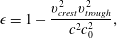 $$\begin{eqnarray}\displaystyle \unicode[STIX]{x1D716}=1-\frac{v_{crest}^{2}v_{trough}^{2}}{c^{2}c_{0}^{2}}, & & \displaystyle\end{eqnarray}$$
where
 $v_{trough}$
and
 $c$
denote the fluid speed at the trough and the phase speed in the inertial frame, respectively, was used by Longuet-Higgins (Reference Longuet-Higgins1975). The computational efficiency was drastically improved by using this perturbation quantity. In addition, Longuet-Higgins (Reference Longuet-Higgins1975) proposed an alternative expansion parameter
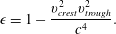 $$\begin{eqnarray}\displaystyle \unicode[STIX]{x1D716}=1-\frac{v_{crest}^{2}v_{trough}^{2}}{c^{4}}. & & \displaystyle\end{eqnarray}$$
Using (1.3) as the perturbation quantity, Cokelet (Reference Cokelet1977) carried out the expansion to the 120th order, and obtained convergent results for Stokes waves with
 $d/\unicode[STIX]{x1D706}>0.0168$
. However, Cokelet (Reference Cokelet1977) pointed out that his method cannot give accurate wave profiles even in cases of
 $d/\unicode[STIX]{x1D706}<0.11$
. Furthermore, Dallaston & Mccue (Reference Dallaston and Mccue2010) reconsidered both Schwartz’s (Schwartz Reference Schwartz1974) and Cokelet’s (Cokelet Reference Cokelet1977) schemes, but with exact calculations so as to void any round-off error. However, they found that both the series expansions of Schwartz (Reference Schwartz1974) and Cokelet (Reference Cokelet1977) actually cannot provide precise estimates of the limiting wave properties in extremely shallow water.
Besides perturbation methods (Schwartz Reference Schwartz1974; Cokelet Reference Cokelet1977), a variety of numerical methods were proposed for the limiting Stokes wave. One common numerical method is to minimize the mean-squared error in the kinematic and dynamic free-surface boundary conditions. Chappelear (Reference Chappelear1961) expanded the velocity and the profile equation in Fourier series, and then used the method of least squares to determine the Fourier coefficients. Dean (Reference Dean1965) employed an analytical streamfunction expression with a series of unknown coefficients to describe the waves, and then used a numerical perturbation method to determine the unknown coefficients. Similarly, the numerical method was used by Williams (Reference Williams1981) to minimize the error in the surface boundary conditions over a series of evenly spaced points. However, a new crest term was supplemented to the integral equation in Williams’ numerical method. Williams (Reference Williams1981) found that introducing this new term can greatly accelerate the convergence, i.e. the same level of accuracy can be reached by fewer Fourier coefficients. This method (Williams Reference Williams1981) was a significant progress in numerics for Stokes’ wave, since it is one of the few methods that are both free from extrapolation and can give accurate results. Unfortunately, this method (Williams Reference Williams1981) still fails for extremely shallow water
 $d/\unicode[STIX]{x1D706}<0.0168$
.
Rienecker & Fenton (Reference Rienecker and Fenton1981) used a finite Fourier series to reduce the free-surface conditions to a set of nonlinear algebraic equations, and then used Newton’s iteration method to solve these nonlinear equations. By means of this method, the equations are satisfied identically at a number of points on the surface. This method was further simplified by Fenton (Reference Fenton1988) who numerically solved all the necessary partial derivatives. However, Fenton (Reference Fenton1988) found that it is sometimes still necessary first to solve a sequence of lower waves and then to extrapolate forward in height steps to reach the desired height. Vanden-Broeck & Schwartz (Reference Vanden-Broeck and Schwartz1979) proposed an efficient numerical scheme to solve the steep gravity wave. They first formulated the steep gravity waves as a system of integro-differential equations, and then used Newton’s iteration technique to solve the coupled equations. Using this numerical method, accurate results can be obtained even in the case of
 $d/\unicode[STIX]{x1D706}=0.008$
. In addition, Vanden-Broeck & Miloh (Reference Vanden-Broeck and Miloh1995) employed series truncation methods, which use a refinement of Davies–Tulin’s approximation (Davies Reference Davies1951; Tulin Reference Tulin1983), to solve the steep gravity waves. By means of these methods, accurate numerical results can be obtained in the cases of
 $d/\unicode[STIX]{x1D706}\geqslant 0.0168$
. It should be emphasized that these schemes are easier to implement than the boundary integral equation methods (Hunter & Vanden-Broeck Reference Hunter and Vanden-Broeck1983).
Besides the property of limiting Stokes wave with a included
 $120^{\circ }$
angle in the crest, the non-monotonicity of the speed and energy near the limiting wave height, first found by Longuet-Higgins (Reference Longuet-Higgins1975), also received wide attention from researchers. Longuet-Higgins & Fox (Reference Longuet-Higgins and Fox1978) proposed a matching technique for gravity waves of almost extreme form, and then successfully confirmed the existence of branch points of order
 $1/2$
, as predicted by Grant (Reference Grant1973), and of turning points in the phase velocity as a function of wave height. In addition, the asymptotic solution of Longuet-Higgins & Fox (Reference Longuet-Higgins and Fox1978) indicates that there is an infinite number of turning points in the dispersion relation, momentum and energy for the wave height very close to the maximum height. However, many methods generally only capture one or two of these turning points (Chandler & Graham Reference Chandler and Graham1993), although three turning points are found by Dallaston & Mccue (Reference Dallaston and Mccue2010).
Note that understanding the characterization of the singularity structure of the Stokes wave, such as the locations and scalings of the singularities, is of great help in theory (Tanveer Reference Tanveer1991; Crew & Trinh Reference Crew and Trinh2016). Dyachenko, Lushnikov & Korotkevich (Reference Dyachenko, Lushnikov and Korotkevich2014, Reference Dyachenko, Lushnikov and Korotkevich2016) analysed the distance
 $d_{c}$
from the lowest singularity in the upper half-plane (i.e. the square-root branch point) to the real line which corresponds to the fluid free surface, and then suggested a power law scaling
 $d_{c}\propto (H_{max}-H)^{3/2}$
. Using this power law scaling, Dyachenko et al. (Reference Dyachenko, Lushnikov and Korotkevich2014, Reference Dyachenko, Lushnikov and Korotkevich2016) presented an estimate
 $H_{max}/\unicode[STIX]{x1D706}\approx 0.1410633$
in deep water. Moreover, a square-root branch point is found by Lushnikov (Reference Lushnikov2016) to be the only singularity in the physical (first) sheet of the Riemann surface for a non-limiting Stokes wave. Then an infinite number of square-root singularities are found in the infinite number of non-physical sheets of Riemann surface after crossing a branch cut of a square root into the second and subsequently higher sheets of the Riemann surface. Furthermore, Lushnikov (Reference Lushnikov2016) conjectured that a non-limiting Stokes wave at the leading order consists of the infinite product of nested square-root singularities, and that on increasing the steepness of the Stokes wave to the extreme form, these nested square-root singularities will simultaneously approach the real line from different sheets of Riemann surface and finally form together a
 $2/3$
power law singularity of the limiting Stokes wave. This conjecture was well supported by high precision simulations. In addition, the slow decay of the Fourier coefficients is a challenging problem for numerical methods due to the existence of the singularities for a limiting/approximately limiting Stokes wave. In order to move all complex singularities away from the free surface, Lushnikov et al. (Reference Lushnikov, Dyachenko and Silantyev2017) introduced a free parameter into an auxiliary conformal mapping so as to allow for finer resolution near the crest of the wave. They found that the numerical convergence rate is dramatically improved by adapting the numerical grid near singularities.
Up to now, there are only few methods (Schwartz Reference Schwartz1974; Cokelet Reference Cokelet1977; Vanden-Broeck & Schwartz Reference Vanden-Broeck and Schwartz1979; Williams Reference Williams1981) capable of solving the two-dimensional limiting (extreme) steady progressive wave in very shallow water. Besides, almost all analytic/numerical methods fail to give accurate results (especially for the wave profile) for limiting waves in extremely shallow water, such as
 $d/\unicode[STIX]{x1D706}<0.005$
. In addition, most analytic/numerical methods rely on extrapolation techniques, such as the Padé approximant, so as to accelerate the convergence and remove singularities that limit a series radius of convergence. So, an approach that can yield accurate results for the two-dimensional limiting (extreme) progressive gravity wave in arbitrary water depth without using any kind of extrapolation technique is of great value. This is the motivation of this paper.
In this paper, the limiting Stokes wave in arbitrary water depth is successfully solved by an analytic approximation method, namely the homotopy analysis method (HAM) (Liao Reference Liao1992; Liao Reference Liao1999, Reference Liao2003, Reference Liao2009, Reference Liao2010, Reference Liao2012; Van Gorder & Vajravelu Reference Van Gorder and Vajravelu2008; Kimiaeifar et al.
Reference Kimiaeifar, Lund, Thomsen and Srensen2011; Mastroberardino Reference Mastroberardino2011; Vajravelu & Van Gorder Reference Vajravelu and Van Gorder2012; Sardanyés et al.
Reference Sardanyés, Rodrigues, Januário, Martins, Gil-Gómez and Duarte2015; Liao, Xu & Stiassnie Reference Liao, Xu and Stiassnie2016; Liu, Xu & Liao Reference Liu, Xu and Liao2017, Reference Liu, Xu and Liao2018; Zhong & Liao Reference Zhong and Liao2017, Reference Zhong and Liao2018). Unlike perturbation methods (Schwartz Reference Schwartz1974; Cokelet Reference Cokelet1977), the HAM is independent of any small/large physical parameter. Especially, different from all analytic approximations, there is a so-called ‘convergence-control parameter’
 $\hbar$
in the frame of the HAM, which has no physical meaning but provides a convenient way to guarantee the convergence of series solutions. For example, perturbation techniques are invalid for large deformation of a von Kármán plate, a famous classic problem in solid mechanics. However, Zhong & Liao (Reference Zhong and Liao2017, Reference Zhong and Liao2018) successfully applied the HAM to gain convergent series solutions even for extremely large deformation of a von Kármán plate. It is worthwhile mentioning that some mathematical theorems of convergence have been rigorously proved in the framework of the HAM (Liao Reference Liao2012). For instance, it has been proved by Liao (Reference Liao2012) that the power series given by the HAM
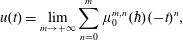 $$\begin{eqnarray}\displaystyle u(t)=\lim _{m\rightarrow +\infty }\mathop{\sum }_{n=0}^{m}\unicode[STIX]{x1D707}_{0}^{m,n}(\hbar )(-t)^{n}, & & \displaystyle\end{eqnarray}$$
where
 $$\begin{eqnarray}\displaystyle \unicode[STIX]{x1D707}_{0}^{m,n}(\hbar )=(-\hbar )^{n}\mathop{\sum }_{k=0}^{m-n}\binom{n-1+k}{k}(1+\hbar )^{k}, & & \displaystyle\end{eqnarray}$$
converges to
 $1/(1+t)$
in the intervals:
 $$\begin{eqnarray}\displaystyle -1<t<-\frac{2}{\hbar }-1,\quad \text{when}\;\hbar <0, & & \displaystyle\end{eqnarray}$$
and
 $$\begin{eqnarray}\displaystyle -\frac{2}{\hbar }-1<t<-1,\quad \text{when}\;\hbar >0, & & \displaystyle\end{eqnarray}$$
respectively. So, the power series (1.4) converges to
 $1/(1+t)$
either in the interval
 $(-1,+\infty )$
if
 $\hbar <0$
tend 0, or in the interval
 $(-\infty ,-1)$
if letting
 $\hbar >0$
tend to 0, respectively. In other words, the power series (1.4) given by the HAM can converge to
 $1/(1+t)$
in its entire definition interval (except the singularity
 $t=-1$
) by properly choosing the so-called ‘convergence-control parameter’
 $\hbar$
. This is a good example to illustrate that the HAM can dramatically improve the convergence of a series by means of the so-called convergence-control parameter. By contrast, the traditional power series:
 $$\begin{eqnarray}\displaystyle \frac{1}{1+t}\sim 1-t+t^{2}-t^{3}+t^{4}-\cdots & & \displaystyle\end{eqnarray}$$
only converges in the interval
 $(-1,1)$
. Thus, the HAM can indeed greatly enlarge the convergence interval of solution series by means of properly choosing the so-called ‘convergence-control parameter’
 $\hbar$
. Note that perturbation methods for many problems have been found to be a special case of the HAM when
 $\hbar =-1$
, as illustrated by Zhong & Liao (Reference Zhong and Liao2017, Reference Zhong and Liao2018), and this well explains why perturbation results are often invalid in cases of high nonlinearity. In addition, the HAM provides us with great freedom to choose initial approximation so that iterations can be easily used to accelerate convergence in the framework of the HAM. Besides, a better initial guess can also modify the convergence of iteration, too. More importantly, something completely new/different has been successfully obtained by means of the HAM: the steady-state resonant waves were first predicted by the HAM in theory (Liao Reference Liao2011; Xu et al.
Reference Xu, Lin, Liao and Stiassnie2012; Liu & Liao Reference Liu and Liao2014) and then confirmed experimentally in a laboratory (Liu et al.
Reference Liu, Xu, Li, Peng, Alsaedi and Liao2015): all of these illustrate the novelty and potential of the HAM for highly nonlinear problems.
There exist two challenges for the traditional perturbation methods: (i) the series solutions diverge either when the water depth is rather small or when the wave height approaches the peak value; (ii) the computational efficiency is rather low when the terms of the Fourier coefficients are large. For the first challenge, it is found that the convergence of series solutions of the limiting Stokes wave can be guaranteed by means of choosing a proper convergence-control parameter
 $\hbar$
in the framework of the HAM. Note that, since there is a singularity exactly located at the crest for a Stokes wave of extreme form, considering enough terms of the Fourier series is inevitable if results of high precision are required. For the second challenge, we used an iterative HAM approach to greatly accelerate convergence of all unknown Fourier coefficients. Thus, by means of an iteration HAM approach with a properly chosen convergence-control parameter
 $\hbar$
, accurate results in arbitrary water depth can be obtained efficiently. More importantly, since all Fourier coefficients obtained by the HAM are convergent, accurate wave profiles in very shallow water can be presented without using any kind of extrapolation technique. Compared with the perturbation methods (Schwartz Reference Schwartz1974; Cokelet Reference Cokelet1977), our HAM approach is simpler, easier to use and is valid across almost the whole range of physical parameters, as mentioned later in this paper. All of these demonstrate the superiority of the HAM over the perturbation method for this famous problem in fluid mechanics.
This paper is organized as follows. Fundamental equations are given in § 2. Procedures of the HAM for the limiting Stokes wave problem are presented in § 3. The limiting (extreme) Stokes wave in infinite depth is considered in § 4. The limiting Stokes waves in finite depth are investigated in § 5, with comparison to previous results (Laitone Reference Laitone1960; Fenton Reference Fenton1972; Schwartz Reference Schwartz1974; Cokelet Reference Cokelet1977; Williams Reference Williams1981). Concluding remarks are given in § 6.
2 Mathematical description of the limiting Stokes wave
Consider symmetrical, two-dimensional, periodic gravity waves propagating from right to left in a fluid with a horizontal bottom. The propagation of waves is only under the influence of gravity. Wave speed,
 $c$
, is constant relative to an inertial frame. Assume that the fluid is inviscid and incompressible and that the motion is irrotational. Consider another reference frame moving with a wave crest. With respect to this frame, the motion is steady.
(a)
 $z$
plane, (b)
 $\unicode[STIX]{x1D701}$
plane.
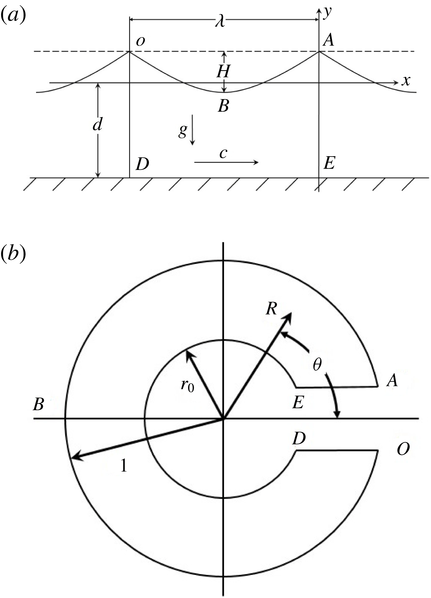
As shown in figure 1(a),
 $\unicode[STIX]{x1D706}$
,
 $H$
,
 $g$
represent the wavelength, the wave height and the gravity acceleration, respectively. Locate the
 $x$
axis at a distance
 $d$
above the bottom. Let the streamfunction
 $\unicode[STIX]{x1D6F9}=0$
on the free surface, and
 $\unicode[STIX]{x1D6F9}=-c\,d$
on the horizontal bottom. The Bernoulli condition on the free surface reads
 $$\begin{eqnarray}\displaystyle v\bar{v}+2gy=K,\quad \unicode[STIX]{x1D6F9}=0, & & \displaystyle\end{eqnarray}$$
where velocity
 $v=v_{x}-\text{i}v_{y}$
, the bar denotes the complex conjugation, and
 $K$
is an unknown constant.
As shown in figure 1, we map the interior of fluid motion ‘ABODEA’ in the physical ‘
 $z$
’ plane into an annulus ‘ABODEA’ in the ‘
 $\unicode[STIX]{x1D701}$
’ plane according to the transformation:
 $$\begin{eqnarray}\displaystyle x+\text{i}y=z(x,y)=z(\unicode[STIX]{x1D701})=\text{i}\left[\text{ln}\unicode[STIX]{x1D701}+\mathop{\sum }_{j=1}^{+\infty }\frac{a_{j}}{j}\left(\unicode[STIX]{x1D701}^{j}-\frac{r_{0}^{2j}}{\unicode[STIX]{x1D701}^{j}}\right)\right], & & \displaystyle\end{eqnarray}$$
where
 $\unicode[STIX]{x1D701}=R\text{e}^{\text{i}\unicode[STIX]{x1D703}}$
;
 $R$
,
 $r_{0}$
and
 $\unicode[STIX]{x1D703}$
represent the radius, inner radius and argument respectively;
 $a_{1},a_{2},\ldots ,a_{j},\ldots$
are unknown constant coefficients to be computed. The horizontal bottom
 $\unicode[STIX]{x1D6F9}=-c\,d$
and the free surface
 $\unicode[STIX]{x1D6F9}=0$
are then mapped onto the circles
 $R=r_{0}=\text{e}^{-d}$
and
 $R=1$
, respectively. Note that
 $r_{0}=0$
and
 $r_{0}=1$
correspond to the cases of infinite depth and infinite shallow water, respectively. The complex velocity potential
 $w$
can be expressed as
 $$\begin{eqnarray}\displaystyle w=\unicode[STIX]{x1D6F7}+\text{i}\unicode[STIX]{x1D6F9}=\text{i}\,c\,\text{ln}\,\unicode[STIX]{x1D701}=c\,\unicode[STIX]{x1D703}+\text{i}\,c\,\text{ln}\,R, & & \displaystyle\end{eqnarray}$$
where
 $\unicode[STIX]{x1D6F7}$
represents velocity potential.
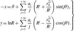
According to (2.2), we have
 $$\begin{eqnarray}\displaystyle \left.\begin{array}{@{}c@{}}\displaystyle -x=\unicode[STIX]{x1D703}+\mathop{\sum }_{j=1}^{+\infty }\frac{a_{j}}{j}\left(R^{j}+\frac{r_{0}^{2j}}{R^{j}}\right)\sin (j\unicode[STIX]{x1D703}),\\ \displaystyle y=\text{ln}R+\mathop{\sum }_{j=1}^{+\infty }\frac{a_{j}}{j}\left(R^{j}-\frac{r_{0}^{2j}}{R^{j}}\right)\cos (j\unicode[STIX]{x1D703}).\end{array}\right\} & & \displaystyle\end{eqnarray}$$
So, we have the wavelength
 $$\begin{eqnarray}\displaystyle \unicode[STIX]{x1D706}=x|_{R=1,\unicode[STIX]{x1D703}=0}-x|_{R=1,\unicode[STIX]{x1D703}=2\unicode[STIX]{x03C0}}=2\unicode[STIX]{x03C0}, & & \displaystyle\end{eqnarray}$$
and the wave steepness
 $$\begin{eqnarray}\displaystyle \frac{H}{\unicode[STIX]{x1D706}}=\frac{1}{2\unicode[STIX]{x03C0}}(y|_{R=1,\unicode[STIX]{x1D703}=0}-y|_{R=1,\unicode[STIX]{x1D703}=\unicode[STIX]{x03C0}})=\mathop{\sum }_{j=1}^{+\infty }\frac{a_{j}}{2j\unicode[STIX]{x03C0}}(1-r_{0}^{2j})[1-\cos (j\unicode[STIX]{x03C0})]. & & \displaystyle\end{eqnarray}$$
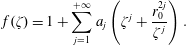
According to (2.3), the complex velocity
 $v$
reads
 $$\begin{eqnarray}\displaystyle v=\frac{\text{d}w}{\text{d}z}=\frac{\text{d}w}{\text{d}\unicode[STIX]{x1D701}}\,\frac{\text{d}\unicode[STIX]{x1D701}}{\text{d}z}=\frac{c}{f(\unicode[STIX]{x1D701})}, & & \displaystyle\end{eqnarray}$$
where
 $$\begin{eqnarray}\displaystyle f(\unicode[STIX]{x1D701})=1+\mathop{\sum }_{j=1}^{+\infty }a_{j}\left(\unicode[STIX]{x1D701}^{j}+\frac{r_{0}^{2j}}{\unicode[STIX]{x1D701}^{j}}\right). & & \displaystyle\end{eqnarray}$$
Note that the velocity at the crest is zero for the highest wave. Using this restriction condition, equation (2.1) becomes
 $$\begin{eqnarray}\displaystyle v\bar{v}+2g\int _{0}^{\unicode[STIX]{x1D703}}\text{Im}\left[\frac{\text{d}z}{\text{d}\unicode[STIX]{x1D701}}\,\frac{\text{d}\unicode[STIX]{x1D701}}{\text{d}\unicode[STIX]{x1D703}}\right]\text{d}\unicode[STIX]{x1D703}=0,\quad \text{when}~\unicode[STIX]{x1D6F9}=0. & & \displaystyle\end{eqnarray}$$
Substituting (2.2), (2.7), (2.8) into (2.9), we have the nonlinear algebraic equation
 $$\begin{eqnarray}\displaystyle \frac{2g}{c^{2}}\,f\,\bar{f}\,\int _{0}^{\unicode[STIX]{x1D703}}\text{Im}[f]\,\text{d}\unicode[STIX]{x1D703}-1=0,\quad \text{at}~R=1. & & \displaystyle\end{eqnarray}$$
Theoretically,
 $a_{1},a_{2},\ldots ,a_{j},\ldots$
need to all be reserved to identically satisfy (2.10). However, we can only consider limited terms in practice. Thus, let us consider here the first
 $r$
Fourier coefficients
 $a_{1},a_{2},\ldots ,a_{r}$
, i.e.
 $f$
is approximated by
 $$\begin{eqnarray}\displaystyle f(\unicode[STIX]{x1D701})\approx a_{0}+\mathop{\sum }_{j=1}^{r}a_{j}\left(\unicode[STIX]{x1D701}^{j}+\frac{r_{0}^{2j}}{\unicode[STIX]{x1D701}^{j}}\right),\quad a_{0}=1. & & \displaystyle\end{eqnarray}$$
Substituting (2.11) into (2.10) and then equating the coefficients of
 $\cos (k\unicode[STIX]{x1D703})$
, where
 $k=0,1,2,\ldots ,r$
, we obtain the following
 $(r+1)$
algebraic equations: (detailed derivation is shown in appendix A)
 $$\begin{eqnarray}\displaystyle c^{2}=g\left(2j_{0}h_{0}+\mathop{\sum }_{n=1}^{r}j_{n}h_{n}\right), & & \displaystyle\end{eqnarray}$$
and
 $$\begin{eqnarray}\displaystyle & & \displaystyle {\mathcal{N}}_{k}[a_{1},a_{2},\ldots ,a_{r}]\nonumber\\ \displaystyle & & \displaystyle \quad =j_{0}h_{k}+j_{k}h_{0}+\frac{1}{2}\left(\mathop{\sum }_{n=1}^{k-1}j_{n}h_{k-n}+\mathop{\sum }_{n=1}^{r-k}j_{n}h_{n+k}+\mathop{\sum }_{n=1}^{r}j_{n+k}h_{n}\right)=0,\end{eqnarray}$$
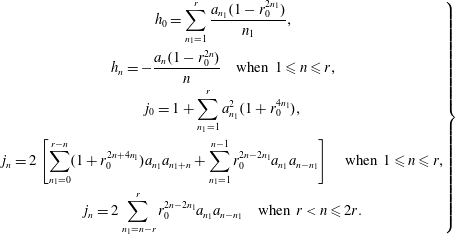
where
 ${\mathcal{N}}_{k}$
(
 $k=1,2,\ldots ,r$
) denotes a nonlinear operator, with the following definitions:
 $$\begin{eqnarray}\displaystyle \left.\begin{array}{@{}c@{}}\displaystyle h_{0}=\mathop{\sum }_{n_{1}=1}^{r}\frac{a_{n_{1}}(1-r_{0}^{2n_{1}})}{n_{1}},\\ \displaystyle h_{n}=-\frac{a_{n}(1-r_{0}^{2n})}{n}\quad \text{when}~1\leqslant n\leqslant r,\\ \displaystyle j_{0}=1+\mathop{\sum }_{n_{1}=1}^{r}a_{n_{1}}^{2}(1+r_{0}^{4n_{1}}),\\ \displaystyle j_{n}=2\left[\mathop{\sum }_{n_{1}=0}^{r-n}(1+r_{0}^{2n+4n_{1}})a_{n_{1}}a_{n_{1}+n}+\mathop{\sum }_{n_{1}=1}^{n-1}r_{0}^{2n-2n_{1}}a_{n_{1}}a_{n-n_{1}}\right]\quad \text{when }1\leqslant n\leqslant r,\\ \displaystyle j_{n}=2\mathop{\sum }_{n_{1}=n-r}^{r}r_{0}^{2n-2n_{1}}a_{n_{1}}a_{n-n_{1}}\quad \text{when }r<n\leqslant 2r.\end{array}\right\} & & \displaystyle\end{eqnarray}$$
Then, the next step is to solve the nonlinear algebraic equations (2.13) for the
 $r$
unknown constant Fourier coefficients
 $a_{1},a_{2},\ldots ,a_{r}$
. Thereafter, the wave speed
 $c$
can be directly given by (2.12).
3 The mathematical approach based on the HAM
Let
 $a_{j,0}$
denote the initial guess of
 $a_{j}~(j=1,2,\ldots ,r)$
,
 $\hbar$
a non-zero auxiliary parameter (called the convergence-control parameter) and
 $q\in [0,1]$
the embedding parameter for a homotopy, respectively. First of all, we construct a family of equations
 $$\begin{eqnarray}\displaystyle (1-q)[\unicode[STIX]{x1D6FA}_{k}(q)-a_{k,0}]=\hbar \,q\,{\mathcal{N}}_{k}[\unicode[STIX]{x1D6FA}_{1}(q),\unicode[STIX]{x1D6FA}_{2}(q),\ldots ,\unicode[STIX]{x1D6FA}_{r}(q)],\quad k=1,2,\ldots ,r, & & \displaystyle\end{eqnarray}$$
where the nonlinear operators
 ${\mathcal{N}}_{1},{\mathcal{N}}_{2},\ldots ,{\mathcal{N}}_{r}$
are defined by (2.13), and the unknown functions
 $\unicode[STIX]{x1D6FA}_{1}(q),\unicode[STIX]{x1D6FA}_{2}(q),\ldots ,\unicode[STIX]{x1D6FA}_{r}(q)$
correspond to the unknown constant Fourier coefficients
 $a_{1},a_{2},\ldots ,a_{r}$
, respectively, and
 $a_{k,0}$
is the initial guess of
 $a_{k}$
. Note that, in the frame of the HAM, we have great freedom to choose the initial guess
 $a_{k,0}$
so that an iteration approach can be proposed based on this kind of freedom to greatly accelerate convergence, as mentioned later. More importantly, the so-called convergence-control parameter
 $\hbar$
can provide us with a simple way to guarantee the convergence of the solution series, as shown below.
Obviously, when
 $q=0$
, equation (3.1) has the solution
 $$\begin{eqnarray}\displaystyle \unicode[STIX]{x1D6FA}_{k}(0)=a_{k,0},\quad k=1,2,\ldots ,r. & & \displaystyle\end{eqnarray}$$
When
 $q=1$
, equation (3.1) is equivalent to the original equation (2.13), provided
 $$\begin{eqnarray}\displaystyle \unicode[STIX]{x1D6FA}_{k}(1)=a_{k},\quad k=1,2,\ldots ,r. & & \displaystyle\end{eqnarray}$$
Therefore, as
 $q$
increases from 0 to 1, the function
 $\unicode[STIX]{x1D6FA}_{j}(q)$
varies (deforms) continuously from the known initial guess
 $a_{j,0}$
to the unknown constant Fourier coefficient
 $a_{j}$
, where
 $j=1,2,\ldots ,r$
. In the frame of the HAM, equation (3.1) is called the zeroth-order deformation equations. Obviously, according to (3.2), we have the Maclaurin series
 $$\begin{eqnarray}\displaystyle \unicode[STIX]{x1D6FA}_{n}(q)=a_{n,0}+\mathop{\sum }_{k=1}^{+\infty }a_{n,k}\,q^{k},\quad n=1,2,\ldots ,r, & & \displaystyle\end{eqnarray}$$
where
 $$\begin{eqnarray}\displaystyle a_{n,k}={\mathcal{D}}_{k}[\unicode[STIX]{x1D6FA}_{n}(q)],\quad n=1,2,\ldots ,r, & & \displaystyle\end{eqnarray}$$
in which
 $$\begin{eqnarray}\displaystyle {\mathcal{D}}_{k}[f]=\left.\frac{1}{k!}\frac{\unicode[STIX]{x2202}^{k}f}{\unicode[STIX]{x2202}q^{k}}\right|_{q=0} & & \displaystyle\end{eqnarray}$$
is called the
 $k$
th-order homotopy derivative of
 $f$
. Note that, according to (3.1),
 $\unicode[STIX]{x1D6FA}_{n}(q)$
and its series (3.4) are dependent upon the so-called convergence-control parameter
 $\hbar$
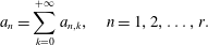
. Assuming that
 $\hbar$
is properly chosen so that the Maclaurin series (3.4) exists and converges at
 $q=1$
, then according to (3.3), we have the so-called homotopy-series solutions
 $$\begin{eqnarray}\displaystyle a_{n}=\mathop{\sum }_{k=0}^{+\infty }a_{n,k},\quad n=1,2,\ldots ,r. & & \displaystyle\end{eqnarray}$$
Substituting (3.4) into the zeroth-order deformation equations (3.1) and then equating the like powers of
 $q$
, we have the so-called
 $m$
th-order deformation equations
 $$\begin{eqnarray}\displaystyle a_{k,m}-\unicode[STIX]{x1D712}_{m}a_{k,m-1}=\hbar \,{\mathcal{D}}_{m-1}[{\mathcal{N}}_{k}],\quad k=1,2,\ldots ,r, & & \displaystyle\end{eqnarray}$$
where
 $$\begin{eqnarray}\displaystyle {\mathcal{D}}_{i}[{\mathcal{N}}_{k}] & = & \displaystyle \mathop{\sum }_{n_{2}=0}^{i}\left\{-\left[\frac{a_{k,i-n_{2}}(1-r_{0}^{2k})}{k}\right]\right.\nonumber\\ \displaystyle & & \displaystyle \times \,\left[1-\unicode[STIX]{x1D712}_{n_{2}+1}+\mathop{\sum }_{n_{1}=1}^{r}\mathop{\sum }_{n_{3}=0}^{n_{2}}(1+r_{0}^{4n_{1}})a_{n_{1},n_{3}}a_{n_{1},n_{2}-n_{3}}\right]\nonumber\\ \displaystyle & & \displaystyle +\,2\left[\mathop{\sum }_{n_{1}=1}^{r}\frac{a_{n_{1},i-n_{2}}(1-r_{0}^{2n_{1}})}{n_{1}}\right]\left[\mathop{\sum }_{n_{1}=1}^{k-1}\mathop{\sum }_{n_{3}=0}^{n_{2}}r_{0}^{2k-2n_{1}}a_{n_{1},n_{3}}a_{k-n_{1},n_{2}-n_{3}}\right.\nonumber\\ \displaystyle & & \displaystyle \left.+\,\mathop{\sum }_{n_{1}=0}^{r-k}\mathop{\sum }_{n_{3}=0}^{n_{2}}(1+r_{0}^{2k+4n_{1}})a_{n_{1},n_{3}}a_{n_{1}+k,n_{2}-n_{3}}\right]\nonumber\\ \displaystyle & & \displaystyle -\,\mathop{\sum }_{n=1}^{k-1}\left[\frac{a_{k-n,i-n_{2}}(1-r_{0}^{2k-2n})}{k-n}\right]\left[\mathop{\sum }_{n_{1}=1}^{n-1}\mathop{\sum }_{n_{3}=0}^{n_{2}}r_{0}^{2n-2n_{1}}a_{n_{1},n_{3}}a_{n-n_{1},n_{2}-n_{3}}\right.\nonumber\\ \displaystyle & & \displaystyle \left.+\,\mathop{\sum }_{n_{1}=0}^{r-n}\mathop{\sum }_{n_{3}=0}^{n_{2}}(1+r_{0}^{2n+4n_{1}})a_{n_{1},n_{3}}a_{n_{1}+n,n_{2}-n_{3}}\right]\nonumber\\ \displaystyle & & \displaystyle -\,\mathop{\sum }_{n=1}^{r-k}\left[\frac{a_{k+n,i-n_{2}}(1-r_{0}^{2k+2n})}{k+n}\right]\left[\mathop{\sum }_{n_{1}=1}^{n-1}\mathop{\sum }_{n_{3}=0}^{n_{2}}r_{0}^{2n-2n_{1}}a_{n_{1},n_{3}}a_{n-n_{1},n_{2}-n_{3}}\right.\nonumber\\ \displaystyle & & \displaystyle \left.+\,\mathop{\sum }_{n_{1}=0}^{r-n}\mathop{\sum }_{n_{3}=0}^{n_{2}}(1+r_{0}^{2n+4n_{1}})a_{n_{1},n_{3}}a_{n_{1}+n,n_{2}-n_{3}}\right]\nonumber\\ \displaystyle & & \displaystyle -\,\mathop{\sum }_{n=1}^{r-k}\left[\frac{a_{n,i-n_{2}}(1-r_{0}^{2n})}{n}\right]\left[\mathop{\sum }_{n_{1}=1}^{n+k-1}\mathop{\sum }_{n_{3}=0}^{n_{2}}r_{0}^{2n+2k-2n_{1}}a_{n_{1},n_{3}}a_{n+k-n_{1},n_{2}-n_{3}}\right.\nonumber\\ \displaystyle & & \displaystyle \left.+\,\mathop{\sum }_{n_{1}=0}^{r-n-k}\mathop{\sum }_{n_{3}=0}^{n_{2}}(1+r_{0}^{2n+2k+4n_{1}})a_{n_{1},n_{3}}a_{n_{1}+n+k,n_{2}-n_{3}}\right]\nonumber\\ \displaystyle & & \displaystyle -\,\mathop{\sum }_{n=r-k+1}^{r}\left[\frac{a_{n,i-n_{2}}(1-r_{0}^{2n})}{n}\right]\nonumber\\ \displaystyle & & \displaystyle \left.\times \,\left[\mathop{\sum }_{n_{1}=n+k-r}^{r}\mathop{\sum }_{n_{3}=0}^{n_{2}}r_{0}^{2n+2k-2n_{1}}a_{n_{1},n_{3}}a_{n+k-n_{1},n_{2}-n_{3}}\right]\right\},\end{eqnarray}$$
in which
 $$\begin{eqnarray}\displaystyle a_{0,0}=1,\quad a_{0,k}=0\quad \text{when}\;k\geqslant 1, & & \displaystyle\end{eqnarray}$$
and
 $$\begin{eqnarray}\displaystyle \unicode[STIX]{x1D712}_{k}=\left\{\begin{array}{@{}ll@{}}0 & \text{when }k\leqslant 1,\\ 1 & \text{when }k>1.\end{array}\right. & & \displaystyle\end{eqnarray}$$
Note that, in the frame of the HAM, we have great freedom to choose the initial guesses
 $a_{1,0},a_{2,0},\ldots ,a_{r,0}$
. So, we can simply choose
 $$\begin{eqnarray}\displaystyle a_{k,0}=\frac{1}{k},\quad k=1,2\ldots ,r. & & \displaystyle\end{eqnarray}$$
Then
 $a_{1,k},a_{2,k},\ldots ,a_{r,k}$
can be obtained by (3.9) step by step, starting from
 $k=1$
. The
 $n$
th-order homotopy approximations of
 $a_{1},a_{2},\ldots ,a_{r}$
read
 $$\begin{eqnarray}\displaystyle \tilde{\unicode[STIX]{x1D6FA}}_{i,n}=\mathop{\sum }_{k=0}^{n}a_{i,k},\quad i=1,2\ldots ,r. & & \displaystyle\end{eqnarray}$$
Once
 $a_{1},a_{2},\ldots ,a_{r}$
are determined, the wave speed
 $c$
can be given by (2.12).
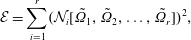
In order to characterize the global error of our HAM approximation, we define the following squared residual error
 $$\begin{eqnarray}\displaystyle {\mathcal{E}}=\mathop{\sum }_{i=1}^{r}({\mathcal{N}}_{i}[\tilde{\unicode[STIX]{x1D6FA}}_{1},\tilde{\unicode[STIX]{x1D6FA}}_{2},\ldots ,\tilde{\unicode[STIX]{x1D6FA}}_{r}])^{2}, & & \displaystyle\end{eqnarray}$$
where the nonlinear operators
 ${\mathcal{N}}_{1},{\mathcal{N}}_{2},\ldots ,{\mathcal{N}}_{r}$
are defined by (2.13). Obviously, the smaller the
 ${\mathcal{E}}$
, the more accurate the HAM approximation (3.13). Besides, it has been proved (Liao Reference Liao2003, Reference Liao2012) in general that a homotopy series converges to solution of original equations as long as all squared residual errors tend to zero. So, it is enough to check the squared residual error (3.14) only.
4 The limiting Stokes wave in infinite depth
To show the validity of our HAM approach mentioned above, we first of all give convergent series solution of the limiting (extreme) Stokes wave in infinite depth.
According to Liao (Reference Liao2003), the convergence of the homotopy-series solutions can be greatly accelerated by introducing the iteration technique, which uses the
 $n$
th-order homotopy approximation
 $\tilde{\unicode[STIX]{x1D6FA}}_{1,n},\tilde{\unicode[STIX]{x1D6FA}}_{2,n},\ldots ,\tilde{\unicode[STIX]{x1D6FA}}_{r,n}$
as new initial guesses
 $a_{1,0},a_{2,0},\ldots ,a_{r,0}$
for the next iteration, say,
 $a_{1,0}=\tilde{\unicode[STIX]{x1D6FA}}_{1,n},a_{2,0}=\tilde{\unicode[STIX]{x1D6FA}}_{2,n},\ldots ,a_{r,0}=\tilde{\unicode[STIX]{x1D6FA}}_{r,n}$
. This provides us with the
 $n$
th-order iteration of the HAM. According to our computation, both the HAM approach without iteration and the HAM-based iteration approach can yield convergent results, but the efficiency of the HAM-based iteration approach is much higher. In particular, the first-order HAM-based iteration approach has the highest efficiency. So, we use the first-order HAM-based iteration approach in all cases of this paper, if not specially mentioned.
Table 1 presents the results in the case of
 $r_{0}=0$
, corresponding to infinite depth of water, given by the convergence-control parameter
 $\hbar =-0.2$
,
 $r=100$
(i.e. one hundred truncated terms of Fourier series) and the initial guess (3.12). Note that the squared residual error
 ${\mathcal{E}}$
defined by (3.14) quickly decreases to the tiny level
 $10^{-17}$
. This illustrates that all Fourier coefficients
 $a_{1},a_{2},\ldots ,a_{100}$
, given by our HAM approach, are convergent.
The squared residual error
 ${\mathcal{E}}$
, wave steepness
 $H/\unicode[STIX]{x1D706}$
and wave speed parameter
 $(g\unicode[STIX]{x1D706})/(2\unicode[STIX]{x03C0}c^{2})$
versus iteration times in the case of
 $r_{0}=0$
, given by the first-order HAM-based iteration approach using
 $c_{0}=-0.2$
,
 $r=100$
and the initial guess (3.12).
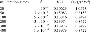
Figure 2 shows the homotopy approximation of the first Fourier coefficient,
 $a_{1}$
, versus iteration times in the case of
 $r_{0}=0$
, given by
 $r=100$
and the convergence-control parameter
 $\hbar =-0.4,-0.25,-0.1$
. Note that
 $\hbar =-0.4$
leads to divergence of iteration,
 $\hbar =-0.25$
corresponds to a quickly convergent iteration but
 $\hbar =-0.1$
a slowly convergent iteration. Obviously, the optimal value of
 $\hbar$
corresponds to the fastest convergence, as pointed out by Liao (Reference Liao2010). It is found that convergent results can be obtained by our iteration HAM approach with arbitrary values of
 $\hbar \in [-0.27,0)$
. So, the convergence-control parameter
 $\hbar$
indeed provides us with a simple way to guarantee convergence and to accelerate convergence. This clearly illustrates the important role of the convergence-control parameter
 $\hbar$
in the framework of the HAM.
The first Fourier coefficient,
 $a_{1}$
, versus number of iterations,
 $n$
, in the case of
 $r_{0}=0$
, given by the first-order HAM-based iteration approach using
 $r=100$
and the convergence-control parameter
 $\hbar =-0.1,-0.25,-0.4$
. – – –,
 $\hbar =-0.1$
; ——,
 $\hbar =-0.25$
; — ⋅ —,
 $\hbar =-0.4$
.
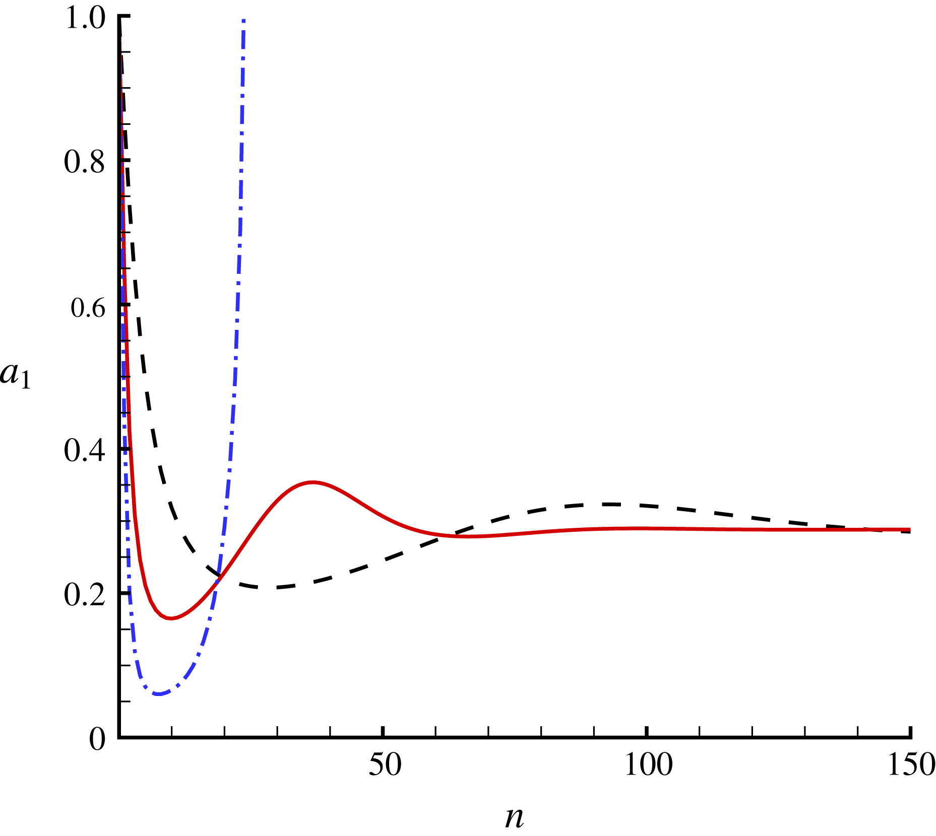
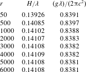
Table 2 presents the convergence results in the case of
 $r_{0}=0$
, given for different
 $r$
. Note that the steepness of the limiting wave in infinite water depth tends to a fixed value
 $H/\unicode[STIX]{x1D706}=0.14108$
when
 $r$
is large enough, say,
 $r>5000$
. This is reasonable, since the precision of our results is controlled by
 $r$
, i.e. the truncated number of the Fourier series (2.11). Note that Schwartz (Reference Schwartz1974) gave
 $H_{max}/\unicode[STIX]{x1D706}=0.14118$
but Dyachenko et al. (Reference Dyachenko, Lushnikov and Korotkevich2016) gave
 $H_{max}/\unicode[STIX]{x1D706}=0.141058$
for a limiting wave in deep water, with 0.071 % and 0.016 % relative errors compared to our results, respectively. It should be emphasized that, by means of the HAM, convergent results of all Fourier coefficients
 $a_{j}$
can be obtained. This distinguishes the HAM from other methods.
Wave steepness
 $H/\unicode[STIX]{x1D706}$
and wave speed parameter
 $(g\unicode[STIX]{x1D706})/(2\unicode[STIX]{x03C0}c^{2})$
versus truncated terms
 $r$
in the case of
 $r_{0}=0$
(in infinite depth), given by the first-order HAM-based iteration approach using
 $c_{0}=-0.2$
.
It is found that the high-order Fourier coefficients
 $a_{j}$
drop rather slowly (e.g.
 $a_{1}=0.29223$
,
 $a_{100}=0.01576$
,
 $a_{500}=0.005415$
,
 $a_{1000}=0.003739$
,
 $a_{3000}=0.002905$
,
 $a_{5000}=0.002759$
). We have
 $H/\unicode[STIX]{x1D706}=0.14085$
even by means of
 $r=500$
, and have the more accurate result
 $H/\unicode[STIX]{x1D706}=0.14108$
by
 $r>5000$
. All of these indicate that
 $f$
defined by (2.8) converges slowly indeed. However, it should be emphasized that, whatever
 $r$
we choose, convergent values of all Fourier coefficients
 $a_{j}$
can be directly obtained by our iterative HAM approach without using any extrapolation or Padé approximant techniques.
Wave profiles in the case of
 $r_{0}=0$
. ——, given by the first-order HAM-based iteration approach; ○, given by the numerical approach of Dyachenko et al. (Reference Dyachenko, Lushnikov and Korotkevich2016); ▴, given by Schwartz’s perturbation method with the aid of a so-called series completion method (Schwartz Reference Schwartz1974).
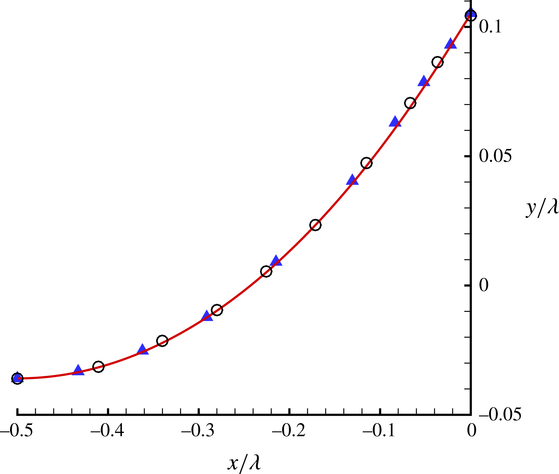
Figure 3 shows the comparison of limiting wave profiles given by Schwartz (Reference Schwartz1974), Dyachenko et al. (Reference Dyachenko, Lushnikov and Korotkevich2016) and our HAM approach. The agreement between them is satisfactory. This indicates the validity of our HAM-based approach. Our limiting wave profile has a sharply pointed crest with an enclosing angle
 $119.3^{\circ }$
, which is very close to the theoretical value
 $120^{\circ }$
. However, Schwartz (Reference Schwartz1974) mentioned that ‘while the method of Páde fractions yields accurate profiles for wave heights somewhat short of the maximum, it is insufficient for the description of very high waves’, and that ‘Páde fractions do not converge well in the immediate neighbourhood of branch-points; moreover, only the first few coefficients
 $a_{j}$
, can be determined with acceptable accuracy’. Thus, Schwartz (Reference Schwartz1974) had to use the so-called ‘series completion method’ to gain a satisfactory wave profile. By contrast, using the HAM, convergent results of all Fourier coefficients
 $a_{j}~(j=1,2,3,\ldots ,r)$
and the convergent wave profile for the limiting wave can be obtained without using any extrapolation techniques such as the Padé technique, the series completion method and so on. This illustrates that the HAM-based approach is superior to perturbation methods (Schwartz Reference Schwartz1974; Cokelet Reference Cokelet1977). This is mainly because, unlike perturbation methods, the HAM provides us with a convenient way (through the so-called convergence-control parameter
 $\hbar$
) to guarantee the convergence of solution series.
5 The limiting Stokes wave in finite depth
Note that
 $r_{0}=0$
and
 $r_{0}=1$
correspond to the cases of infinite depth and infinitely shallow water, respectively. Without loss of generality, let us first consider the case of
 $r_{0}=0.05$
. In the frame of the HAM, we have great freedom to choose the initial guesses of
 $a_{1},a_{2},\ldots ,a_{r}$
. Considering the continuous variation of
 $a_{1},a_{2},\ldots ,a_{r}$
as
 $r_{0}$
increases from 0 to 1, the convergent values of
 $a_{1},a_{2},\ldots ,a_{5000}$
in the case of
 $r_{0}=0$
, obviously, are much better than (3.12) as the initial guess for the case of
 $r_{0}=0.05$
. In other words, if we have obtained the convergent results of
 $a_{1},a_{2},\ldots ,a_{5000}$
in the case of
 $r_{0}=0$
, then it is better to take
 $$\begin{eqnarray}\displaystyle a_{k,0}=\left\{\begin{array}{@{}ll@{}}a_{k} & \text{when }1\leqslant k\leqslant 5000,\\ a_{5000} & \text{when }k>5000,\end{array}\right. & & \displaystyle\end{eqnarray}$$
as the initial guesses of
 $a_{1},a_{2},\ldots ,a_{r}$
in the case of
 $r_{0}=0.05$
.
It is found that, in the case of
 $r_{0}=0.05$
, the optimal convergence-control parameter
 $\hbar$
is approximately
 $-0.2$
if the initial guess (3.12) for
 $r_{0}=0$
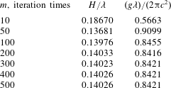
is taken, and 400 iterations are required to gain convergent results
 $H/\unicode[STIX]{x1D706}=0.14026$
and
 $(g\unicode[STIX]{x1D706})/(2\unicode[STIX]{x03C0}c^{2})=0.8421$
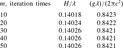
, as shown in table 3. However, if we take the initial guess (5.1), the optimal convergent-control parameter
 $\hbar$
becomes
 $-1.2$
, and we obtain the same convergent results
 $H/\unicode[STIX]{x1D706}=0.14026$
and
 $(g\unicode[STIX]{x1D706})/(2\unicode[STIX]{x03C0}c^{2})=0.8421$
with only thirty iterations, as shown in table 4. Thus, the computational efficiency by means of the initial guess (5.1) is approximately 13 times higher than that by (3.12). This illustrates that our iterative HAM approach with the optimal convergence-control parameter
 $\hbar$
can indeed greatly accelerate the convergence.
Wave steepness
 $H/\unicode[STIX]{x1D706}$
and wave speed parameter
 $(g\unicode[STIX]{x1D706})/(2\unicode[STIX]{x03C0}c^{2})$
versus iterations,
 $m$
, in the case of
 $r_{0}=0.05$
, given by the first-order HAM-based iterative approach using the convergence-control parameter
 $c_{0}=-0.2$
, the truncated terms
 $r=5500$
and the initial guess (3.12).
Wave steepness
 $H/\unicode[STIX]{x1D706}$
and wave speed parameter
 $(g\unicode[STIX]{x1D706})/(2\unicode[STIX]{x03C0}c^{2})$
versus iterations,
 $m$
, in the case of
 $r_{0}=0.05$
, given by the first-order HAM-based iteration approach using the convergence-control parameter
 $c_{0}=-1.2$
, the truncated terms
 $r=5500$
and the initial guesses (5.1).
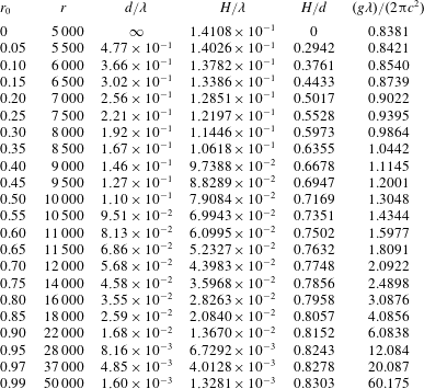
Similarly, the convergent results in arbitrary water depth are successfully obtained by means of the above-mentioned strategy, as shown in table 5. Note that Liao (Reference Liao2010) suggested a general approach to gain an optimal convergence-control parameter in the framework of the HAM. According to our computation, the interval of
 $\hbar$
, which guarantees the convergence of iteration, becomes larger with the increase of
 $r_{0}$
. It is found that, in the case of
 $0.05k<r_{0}\leqslant 0.05(k+1)$
, where
 $0\leqslant k\leqslant 19$
is a natural number, the corresponding optimal convergence-control parameter
 $\hbar$
can be expressed by the following empirical formula
 $$\begin{eqnarray}\displaystyle \hbar =-1.2-\frac{k^{3}}{2000},\quad 0\leqslant k\leqslant 19, & & \displaystyle\end{eqnarray}$$
if we use the known convergent Fourier coefficients
 $a_{j}$
in the case of
 $r_{0}=0.05k$
as the initial guess. Note that a convergence-control parameter
 $\hbar$
closer to 0 represents a slower convergence of solutions, i.e. a lower efficiency of computation, as shown in figure 2. Thus, the convergence-control parameter
 $\hbar$
provides us with a convenient way not only to guarantee the convergence of series solutions but also to improve the computational efficiency. It is found that, for all cases considered in table 5, a few hundred iterations are enough to gain convergent results for all Fourier coefficients
 $a_{j}$
.
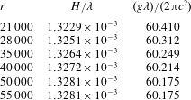
In the case of extremely shallow water, a very large number of Fourier coefficients are needed to present the limiting wave with the sharp crest. Table 6 presents the convergent results given for different values of
 $r$
in the case of
 $r_{0}=0.99$
. It is found that
 $r=50\,000$
can give the fixed results
 $H/\unicode[STIX]{x1D706}=1.3281\times 10^{-3}$
and
 $(g\unicode[STIX]{x1D706})/(2\unicode[STIX]{x03C0}c^{2})=60.175$
in the case of
 $r_{0}=0.99$
. This indicates that our iterative HAM approach can indeed give convergent results for the limiting Stokes waves even in extremely shallow water. Note that, in case of
 $r=50\,000$
, we must solve a set of 50 000 coupled, highly nonlinear algebraic equations! Fortunately, this is possible nowadays by means of a supercomputer such as TH-2 at National Supercomputer Centre in Guangzhou, China. Finally, it should be emphasized that all of these convergent results are obtained directly, without using any extrapolation and Padé approximant techniques.
Results for a variety of water depths, given by the first-order HAM-based iteration approach.
Stokes (Reference Stokes1880) gave a famous conjecture that the limiting wave (with extreme height) should have a sharp crest with an included angle of
 $120^{\circ }$
. Approximately one hundred years later, this conjecture was independently proved in mathematics by Amick, Fraenkel & Toland (Reference Amick, Fraenkel and Toland1982) and Plotnikov (Reference Plotnikov2002) for Stokes waves in an arbitrary depth of water. However, to the best of our knowledge, the detailed wave profiles for the limiting Stokes wave in extremely shallow water have not been reported. Table 7 presents the included crest angles of the limiting Stokes wave in a variety of water depths, given by our iteration HAM approach. All of the included crest angles in different depths given by the HAM are very close to the theoretical value
 $120^{\circ }$
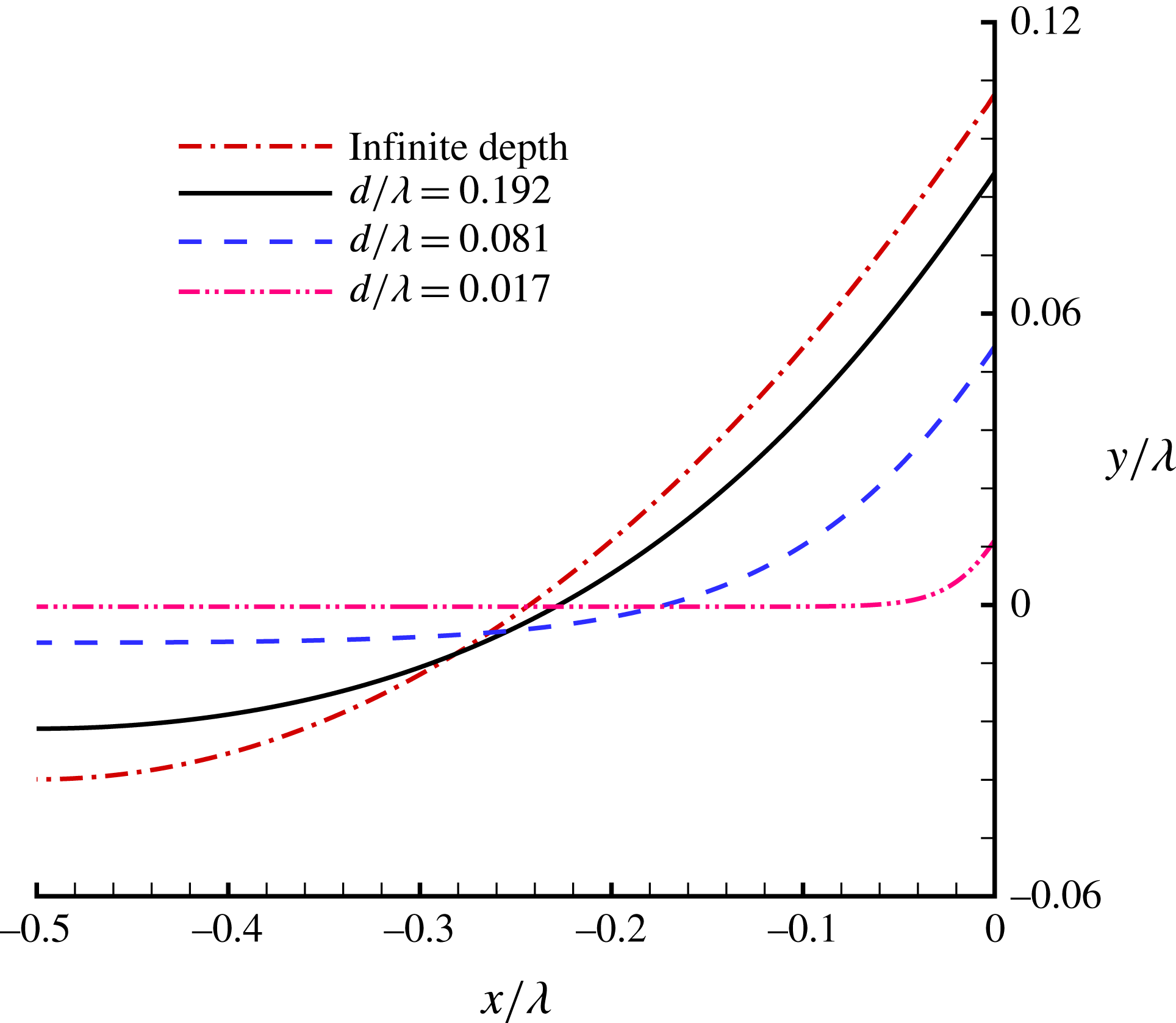
. The wave profiles for a variety of water depths given by the HAM are shown in figure 4. Note that the high-order Fourier coefficients
 $a_{j}$
play an important role in correctly describing the wave profile, especially the wave crest. For instance, although Cokelet’s perturbation method (Cokelet Reference Cokelet1977) can give
 $H/d$
with acceptable accuracy for
 $r_{0}<0.9$
, it fails to give an accurate wave profile even for
 $r_{0}>0.5$
. Fortunately, the HAM can always yield convergent results for all Fourier coefficients by means of choosing a proper convergence-control parameter
 $\hbar$
. This once again illustrates the superiority of the HAM over other methods (Schwartz Reference Schwartz1974; Cokelet Reference Cokelet1977).
Wave steepness
 $H/\unicode[STIX]{x1D706}$
and wave speed parameter
 $(g\unicode[STIX]{x1D706})/(2\unicode[STIX]{x03C0}c^{2})$
versus truncated terms
 $r$
in the case of
 $r_{0}=0.99$
, given by the first-order HAM-based iteration approach.
Included crest angles in a variety of depths, given by the first-order HAM-based iteration approach.

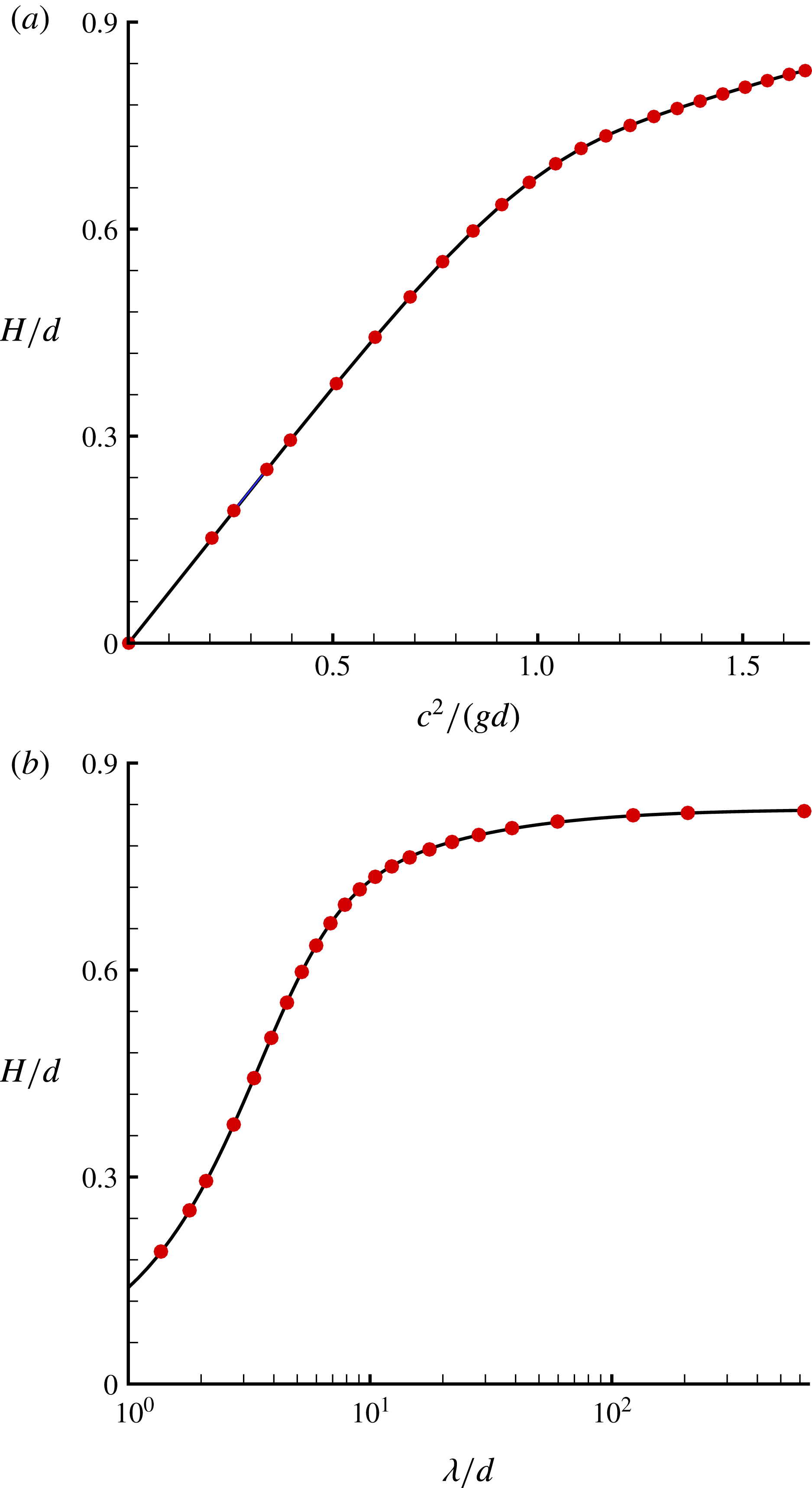
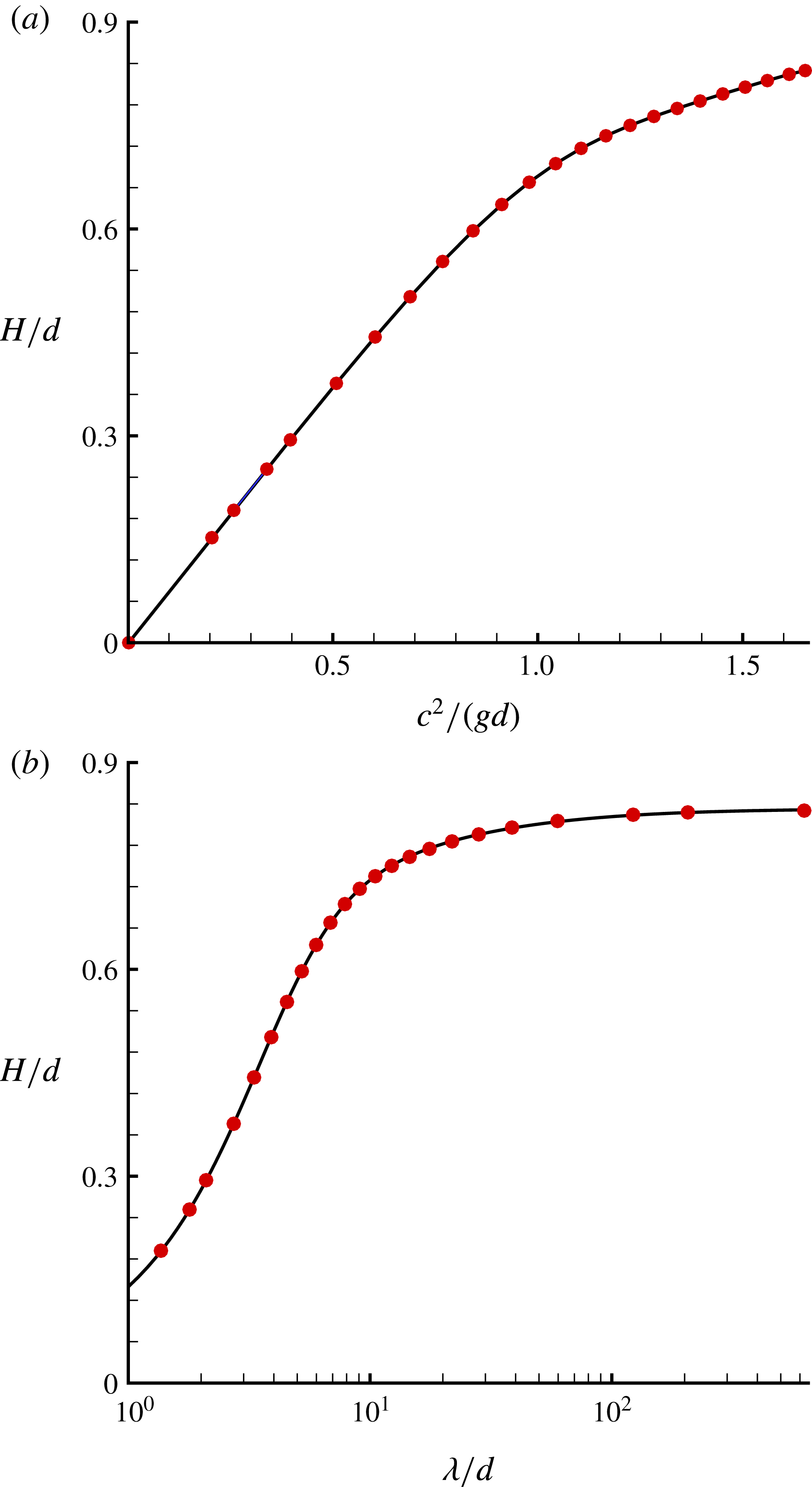
According to the convergent results given by the iterative HAM approach, we have the fitted formulas of
 $H/d$
versus
 $c^{2}/(gd)$
and
 $\unicode[STIX]{x1D706}/d$
:
 $$\begin{eqnarray}\displaystyle \frac{H}{d} & = & \displaystyle 0.58557\,\frac{c^{2}}{gd}+0.62667\left(\frac{c^{2}}{gd}\right)^{2}-0.73410\left(\frac{c^{2}}{gd}\right)^{3}+0.19634\left(\frac{c^{2}}{gd}\right)^{4},\end{eqnarray}$$
 $$\begin{eqnarray}\displaystyle \frac{H}{d} & = & \displaystyle \frac{\displaystyle 0.14109\,\frac{\unicode[STIX]{x1D706}}{d}+0.00804\left(\frac{\unicode[STIX]{x1D706}}{d}\right)^{2}+0.00949\left(\frac{\unicode[STIX]{x1D706}}{d}\right)^{3}}{\displaystyle 1+0.09671\,\frac{\unicode[STIX]{x1D706}}{d}+0.02695\left(\frac{\unicode[STIX]{x1D706}}{d}\right)^{2}+0.01139\left(\frac{\unicode[STIX]{x1D706}}{d}\right)^{3}},\end{eqnarray}$$
which agree quite well with our HAM results, as shown in figure 5.
Wave profiles for a variety of water depths, given by the first-order HAM-based iteration approach.

Let us make some comparisons of the limiting Stokes waves given by different analytic/numerical methods. Table 8 presents the comparison of limiting wave steepness for a variety of depths. The results of Schwartz (Reference Schwartz1974) are accurate only for
 $r_{0}<0.7$
; the results of Cokelet (Reference Cokelet1977) are accurate only for
 $r_{0}\leqslant 0.8$
; the results of Williams (Reference Williams1981) are of high accuracy for
 $r_{0}\leqslant 0.9$
, although they are slightly smaller. However, all of these methods fail to give convergent result for
 $r_{0}>0.9$
, i.e. extremely shallow water. Fortunately, the HAM can give convergent results for the limiting waves for almost arbitrary depth.
Limiting wave steepness,
 $H/\unicode[STIX]{x1D706}$
, for a variety of depths.
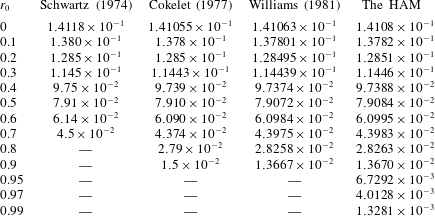
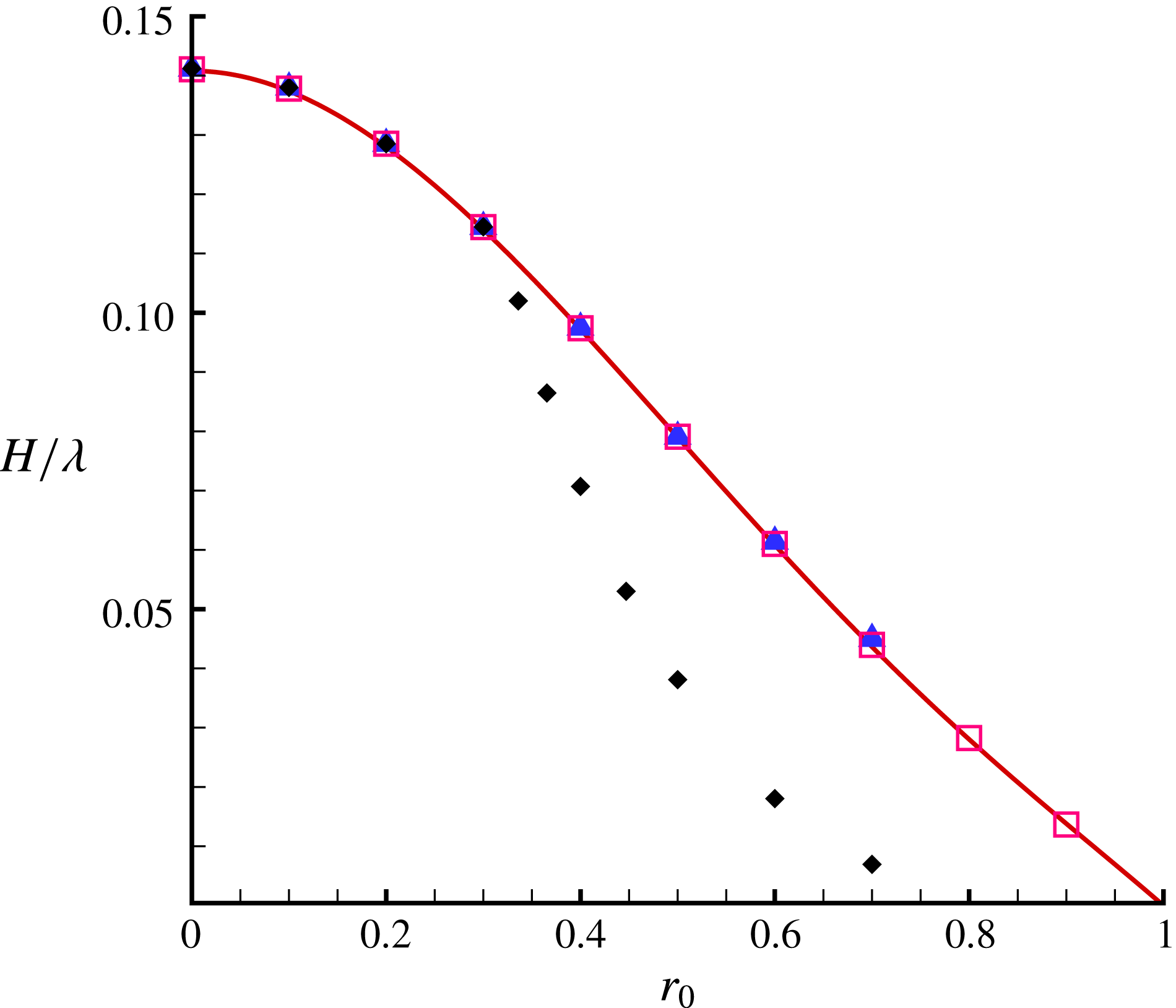
Figure 6 shows the comparison of the limiting wave steepness
 $H/\unicode[STIX]{x1D706}$
, given by Schwartz (Reference Schwartz1974), Williams (Reference Williams1981) and the HAM approach mentioned in this paper. It is found that the perturbation method (Schwartz Reference Schwartz1974) is only valid for
 $r_{0}\in [0,0.7]$
even with the aid of extrapolation and Padé approximant techniques; Williams’ numerical method (Williams Reference Williams1981) is only valid for
 $r_{0}\in [0,0.9]$
. However, the HAM can give accurate convergent results even for
 $r_{0}\in [0,0.99]$
.
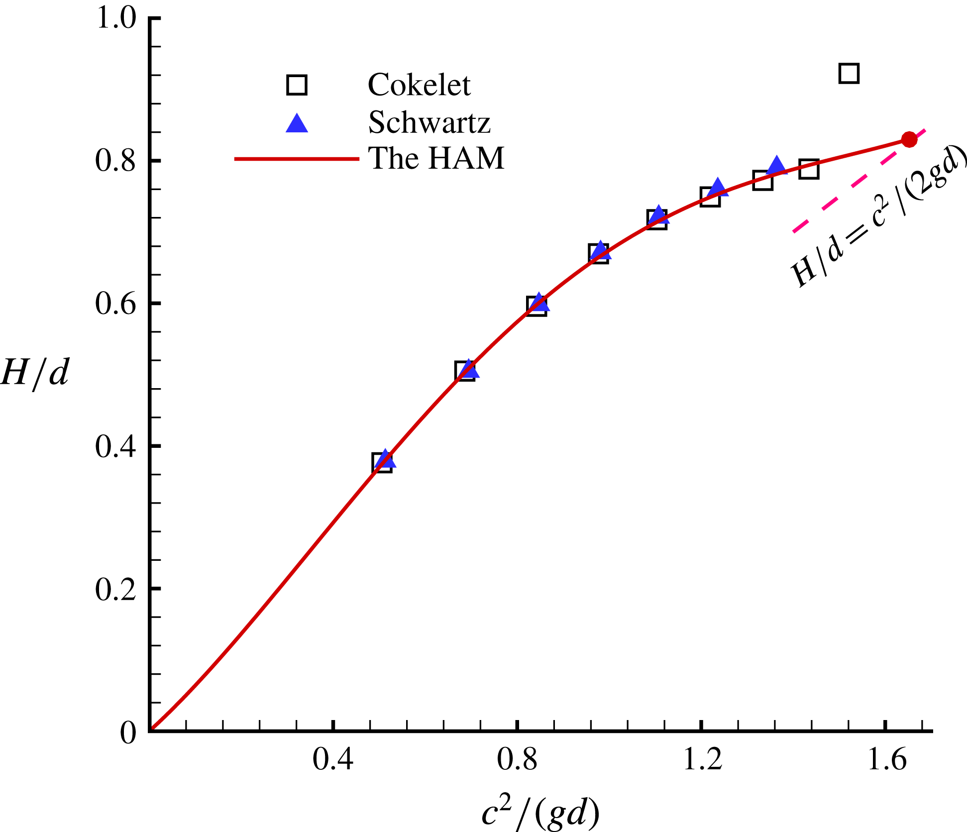
Figure 7 shows the comparison of
 $H/d$
versus the squared Froude number,
 $c^{2}/(gd)$
. It is found that Cokelet’s perturbation method (Cokelet Reference Cokelet1977) fails in extremely shallow water, i.e.
 $r_{0}\geqslant 0.9$
. By contrast, our results given by the HAM are valid in almost arbitrary water depth. Besides, in the case of
 $r_{0}=0.99$
,
 $H/d$
given by the HAM is in accord with the results of the highest solitary wave:
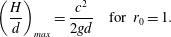 $$\begin{eqnarray}\displaystyle \left(\frac{H}{d}\right)_{max}=\frac{c^{2}}{2gd}\quad \text{for }r_{0}=1. & & \displaystyle\end{eqnarray}$$
This suggests that the solitary wave theory could be unified into the Stokes wave theory.
Comparison of the limiting wave steepness
 $H/\unicode[STIX]{x1D706}$
. ——, the first-order HAM-based iteration approach; ♦, perturbation method with the aid of Padé approximants (Schwartz Reference Schwartz1974); ▴, perturbation method with the aid of both Padé approximants and Shanks’ iterated
 $e_{1}$
transformation (Schwartz Reference Schwartz1974); ▫: Williams’ numerical method (Williams Reference Williams1981).
Comparison of
 $H/d$
, versus the squared Froude number,
 $c^{2}/(gd)$
. ——, the first-order HAM-based iteration approach; ●, the case of
 $r_{0}=0.99$
given by the first-order HAM-based iteration approach; ▴, Schwartz (Reference Schwartz1974); ▫, Cokelet (Reference Cokelet1977); — — —,
 $H/d=c^{2}/(2gd)$
.
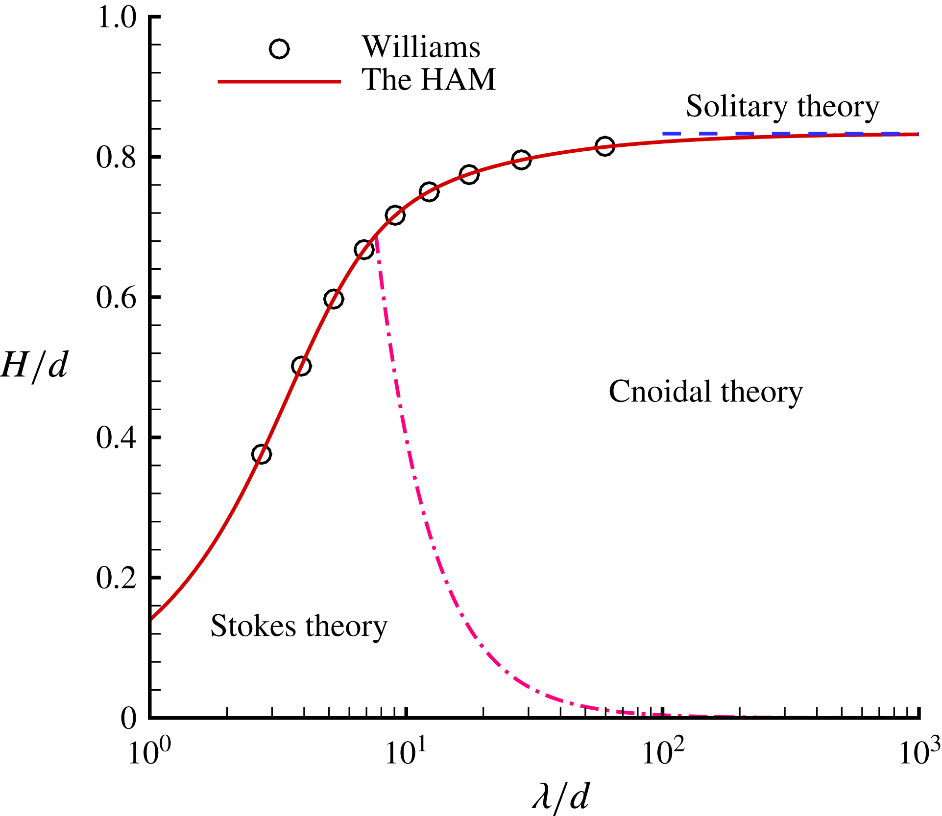
According to Hedges (Reference Hedges1995), waves with the Ursell number
 $H\unicode[STIX]{x1D706}^{2}/d^{3}>4000$
are regarded as solitary waves. It is found that, in the case of
 $r_{0}=0.99$
, corresponding to
 $\unicode[STIX]{x1D706}/d\approx 600$
, the
 $H\unicode[STIX]{x1D706}^{2}/d^{3}$
of the limiting Stokes wave given by the HAM reaches
 $3\times 10^{5}$
. Thus, the Stokes wave theory is actually valid for almost arbitrary depth, as shown in figure 8. So, in the framework of the HAM, the Stokes wave theory can describe not only the periodic waves in deep and intermediate water but also cnoidal waves in shallow water and solitary waves in extremely shallow water.
In addition, the ratio of wave height to depth,
 $H/d$
, of the highest solitary wave has been widely studied by many researchers:
 $H/d=0.827$
was given by Yamada (Reference Yamada1957), Lenau (Reference Lenau1966), Yamada & Shiotani (Reference Yamada and Shiotani1968), Longuet-Higgins & Fenton (Reference Longuet-Higgins and Fenton1974); but
 $H/d=0.8332$
was given by Williams (Reference Williams1981), Witting (Reference Witting1981), Witting & Bergin (Reference Witting and Bergin1981), Hunter & Vanden-Broeck (Reference Hunter and Vanden-Broeck1983). Note that,
 $H/d=0.8303>0.827$
is given by the HAM in the case of
 $r_{0}=0.99$
. Hence the value
 $H/d=0.827$
for the highest solitary wave is denied by the HAM.
Comparison of
 $H/d$
, versus
 $\unicode[STIX]{x1D706}/d$
.
 $\circ$
, Williams (Reference Williams1981); ——, the first-order HAM-based iteration approach; — ⋅ —, demarcation line between Stokes and cnoidal theories, the Ursell number
 $H\unicode[STIX]{x1D706}^{2}/d^{3}=40$
(Hedges Reference Hedges1995); – – –,
 $(H/d)_{max}=0.83322$
for solitary wave (Hunter & Vanden-Broeck Reference Hunter and Vanden-Broeck1983).
Wave profile in the case of
 $r_{0}=0.99$
. – – –, exact solution of KdV equation (Korteweg & de Vries Reference Korteweg and de Vries1895); –
 $\cdot \,\cdot$
–, Laitone’s second-order approximation solution (Laitone Reference Laitone1960); — ⋅ —, Fenton’s ninth-order approximation solution (Fenton Reference Fenton1972); ——, homotopy approximation solution of (2.10).
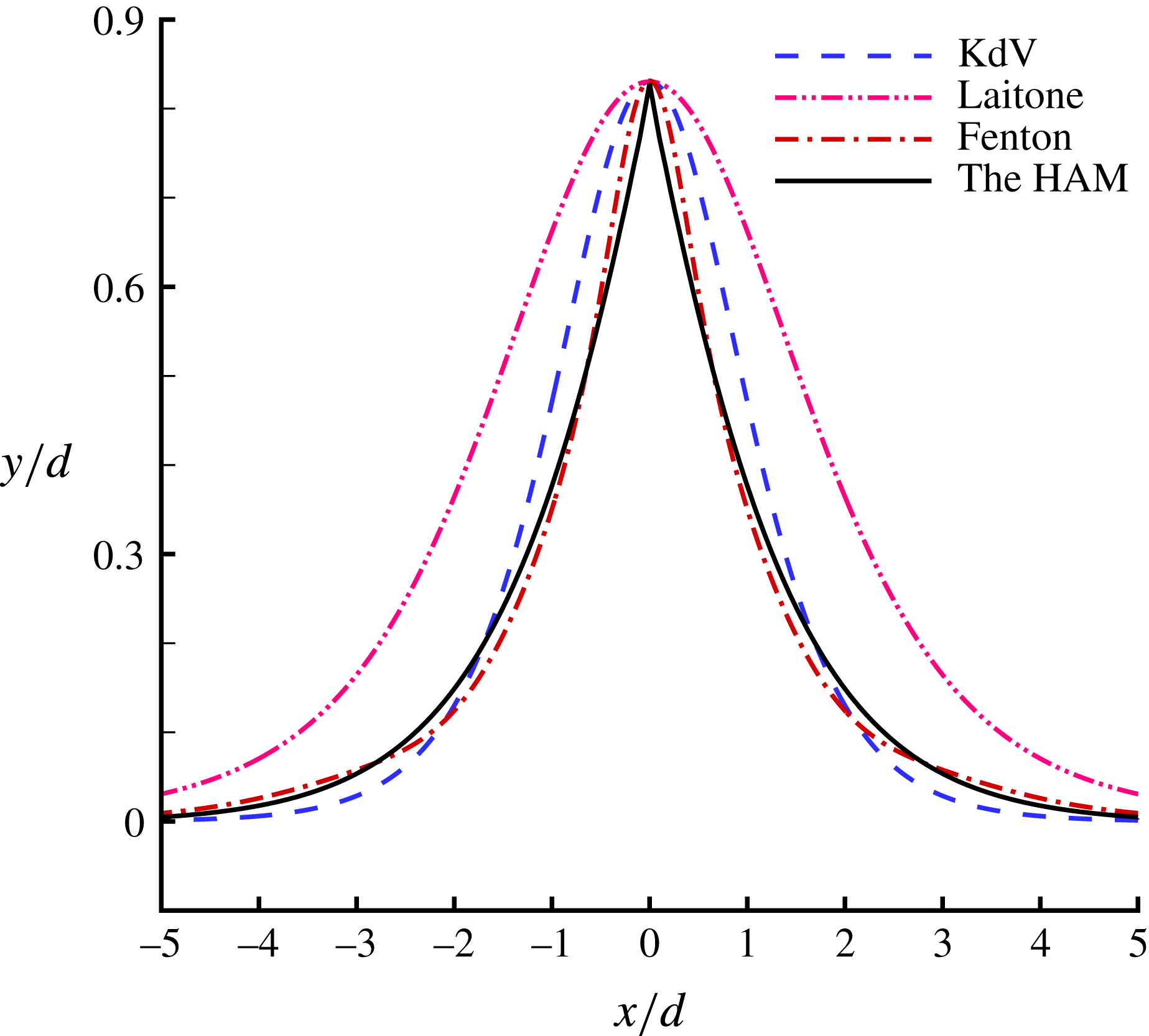
Figure 9 shows the wave profiles of the limiting wave in the case of
 $r_{0}=0.99$
given by the HAM from the exact wave equations, the KdV solution (Korteweg & de Vries Reference Korteweg and de Vries1895), Laitone’s second-order solution (Laitone Reference Laitone1960) and Fenton’s ninth-order solution (Fenton Reference Fenton1972). It is found that only the HAM gives a wave profile with a sharply pointed crest, enclosing an angle
 $119.2^{\circ }$
. So, the KdV solution (Korteweg & de Vries Reference Korteweg and de Vries1895), Laitone’s solution (Laitone Reference Laitone1960) and Fenton’s solution (Fenton Reference Fenton1972) are all no longer valid in the limiting case. However, compared to the famous solitary solution of the KdV equation (Korteweg & de Vries Reference Korteweg and de Vries1895) and Laitone’s solution (Laitone Reference Laitone1960), Fenton’s ninth-order solution (Fenton Reference Fenton1972) is of higher accuracy.
In summary, using the iterative HAM approach with a proper convergence-control parameter, we gain limiting Stokes waves for almost arbitrary water depth, without using any extrapolation techniques. Therefore, in the framework of the HAM, the Stokes wave theory is a unified theory for all kinds of progressive waves in arbitrary depth, even including solitary waves in extremely shallow water.
6 Concluding remarks
Obviously, the limiting Stokes wave in shallow water is a strongly nonlinear problem. Previous methods, especially the perturbation methods, usually suffer divergence either when the wave height approaches the peak value or when the water depth is extremely small. For the limiting Stokes wave, due to the existence of a singularity located exactly at the crest, perturbation methods usually can yield convergent results only for a small part of Fourier coefficients so that the extrapolation methods such as Padé approximant techniques and Shanks’ transformation have to be used.
In this paper, we employ the homotopy analysis method (HAM) to solve the limiting Stokes wave in an arbitrary depth of water. It is found that the convergence of all Fourier coefficients of the solutions can be guaranteed by choosing a proper convergence-control parameter
 $\hbar$
in the framework of the HAM, as shown in figure 2. In addition, since the Fourier series is used to represent the free surface with a sharp pointed crest, using a large number of Fourier coefficients is inevitable. For other analytic/numerical methods, this might lead to rather slow convergence of the Fourier coefficients of the solutions. Fortunately, the HAM also provides us with great freedom to choose the initial guesses of solutions. Based on this kind of freedom of the HAM, we proposed an iteration HAM approach to greatly accelerate the convergence of all Fourier coefficients. Note that, since we consider a large enough number of Fourier coefficients, and more importantly, all of these coefficients are convergent without using any extrapolation methods, we can obtain the accurate wave profile even in rather shallow water.
It should be emphasized that accurate representation of the wave profile in very shallow water is impossible using other methods, especially without using any kind of extrapolation technique. For instance, although Cokelet’s perturbation method (Cokelet Reference Cokelet1977) can give results of
 $H/\unicode[STIX]{x1D706}$
with acceptable accuracy for
 $r_{0}<0.9$
, it can only give a good wave profile for
 $r_{0}\leqslant 0.5$
. Fortunately, by means of the HAM, we gain accurate limiting wave profiles in almost arbitrary depths of water, i.e. from
 $r_{0}=0$
to
 $r_{0}=0.99$
, without using any extrapolation methods such as Padé approximant techniques and Shanks’ transformation. To the best of our knowledge, an accurate wave profile in the case of
 $r_{0}=0.99$
has been never reported. This once again illustrates the superiority of the HAM over perturbation and traditional numerical methods for this famous problem.
According to Hedges (Reference Hedges1995), waves with the Ursell number
 $H\unicode[STIX]{x1D706}^{2}/d^{3}>4000$
are regarded as solitary waves. It is found that, in the case of
 $r_{0}=0.99$
, corresponding to
 $\unicode[STIX]{x1D706}/d\approx 600$
, the
 $H\unicode[STIX]{x1D706}^{2}/d^{3}$
of the Stokes wave given by our HAM approach reaches
 $3\times 10^{5}$
. Thus, the Stokes wave theory is actually valid almost in arbitrary depth, as shown in figure 8. So in the frame of the HAM, the Stokes wave theory can describe not only the periodic waves in deep and intermediate water but also cnoidal waves in shallow water and solitary waves in extremely shallow water. Therefore, in the framework of the HAM, the Stokes wave is a unified theory for all kinds of progressive waves, even including the limiting (extreme) solitary waves with a sharp crest of
 $120^{\circ }$
angle in extremely shallow water!
Note that cubic relations between
 $a_{j}$
in (2.12)–(2.13) were considered in this paper, although quadratic relations between the Fourier coefficients
 $a_{j}$
were reported by Longuet-Higgins (Reference Longuet-Higgins1978). Certainly, the computational efficiency could be improved by means of using the quadratic relations (Longuet-Higgins Reference Longuet-Higgins1985; Balk Reference Balk1996), but one should obtain the same results as mentioned above in this paper, from a physical viewpoint.
From viewpoint of applied mathematics, this paper provides us with an additional example to illustrate that the HAM can indeed be applied to find something completely new, such as the discovery of the steady-state exactly/nearly resonant gravity waves with a time-independent wave spectrum (Liao Reference Liao2011; Xu et al. Reference Xu, Lin, Liao and Stiassnie2012; Liu & Liao Reference Liu and Liao2014; Liu et al. Reference Liu, Xu, Li, Peng, Alsaedi and Liao2015; Liao et al. Reference Liao, Xu and Stiassnie2016; Liu et al. Reference Liu, Xu and Liao2018), or to attack some challenging problems with high nonlinearity.
Acknowledgements
Thanks to the anonymous reviewers for their valuable comments. Thanks to Professor Yaosong Chen (Peking University, China) for his suggesting us to attack the limiting Stokes wave in the extremely shallow water by means of the HAM. This work was carried out on TH-2 at National Supercomputer Centre in Guangzhou, China. It is partly supported by National Natural Science Foundation of China (Approval no. 11432009).
Appendix A. Detailed derivation of formulas (2.12)–(2.14)
Rewrite (2.11)
 $$\begin{eqnarray}\displaystyle f(\unicode[STIX]{x1D701})=\mathop{\sum }_{i=-r}^{r}g_{i}\unicode[STIX]{x1D701}^{i}, & & \displaystyle\end{eqnarray}$$
in which
 $$\begin{eqnarray}\displaystyle \left.\begin{array}{@{}c@{}}g_{i}=a_{-i}r_{0}^{-2i}\quad \text{when }i<0,\\ g_{0}=a_{0},\\ g_{i}=a_{i}\quad \text{when }i>0.\end{array}\right\} & & \displaystyle\end{eqnarray}$$
Note that
 $R=1$
on the free surface, i.e.
 $\unicode[STIX]{x1D701}=\text{e}^{\text{i}\unicode[STIX]{x1D703}}$
. We have
 $$\begin{eqnarray}\displaystyle f\,\bar{f} & = & \displaystyle \left(\mathop{\sum }_{i=-r}^{r}g_{i}\unicode[STIX]{x1D701}^{i}\right)\left(\mathop{\sum }_{i=-r}^{r}g_{i}\unicode[STIX]{x1D701}^{-i}\right)\nonumber\\ \displaystyle & = & \displaystyle \mathop{\sum }_{i=-r}^{r}g_{i}^{2}+\mathop{\sum }_{k=1}^{2r}\left[(\unicode[STIX]{x1D701}^{k}+\unicode[STIX]{x1D701}^{-k})\left(\mathop{\sum }_{m=k-r}^{r}g_{m}g_{m-k}\right)\right]\nonumber\\ \displaystyle & = & \displaystyle \mathop{\sum }_{i=-r}^{r}g_{i}^{2}+\mathop{\sum }_{k=1}^{2r}\left[2\left(\mathop{\sum }_{m=k-r}^{r}g_{m}g_{m-k}\right)\cos (k\unicode[STIX]{x1D703})\right]\nonumber\\ \displaystyle & = & \displaystyle \mathop{\sum }_{k=0}^{2r}j_{k}\cos (k\unicode[STIX]{x1D703}),\end{eqnarray}$$
where
 $$\begin{eqnarray}\displaystyle j_{0}=\mathop{\sum }_{i=-r}^{r}g_{i}^{2},\quad j_{k}=2\mathop{\sum }_{m=k-r}^{r}g_{m}g_{m-k},\quad k=1,2,\ldots ,2r. & & \displaystyle\end{eqnarray}$$
In addition, we have
 $$\begin{eqnarray}\displaystyle \int _{0}^{\unicode[STIX]{x1D703}}\text{Im}[f]\,\text{d}\unicode[STIX]{x1D703} & = & \displaystyle \int _{0}^{\unicode[STIX]{x1D703}}\left[\mathop{\sum }_{k=1}^{r}a_{k}(1-r_{0}^{2k})\sin (k\unicode[STIX]{x1D703})\right]\text{d}\unicode[STIX]{x1D703}\nonumber\\ \displaystyle & = & \displaystyle \mathop{\sum }_{k=1}^{r}\frac{a_{k}(1-r_{0}^{2k})}{k}-\mathop{\sum }_{k=1}^{r}\left[\frac{a_{k}(1-r_{0}^{2k})}{k}\cos (k\unicode[STIX]{x1D703})\right]\nonumber\\ \displaystyle & = & \displaystyle \mathop{\sum }_{k=0}^{r}h_{k}\cos (k\unicode[STIX]{x1D703}),\end{eqnarray}$$
where
 $$\begin{eqnarray}\displaystyle h_{0}=\mathop{\sum }_{n_{1}=1}^{r}\frac{a_{n_{1}}(1-r_{0}^{2n_{1}})}{n_{1}},\quad h_{n}=-\frac{a_{n}(1-r_{0}^{2n})}{n},\quad n=1,2,\ldots ,r. & & \displaystyle\end{eqnarray}$$
Then we have
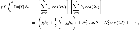 $$\begin{eqnarray}\displaystyle f\,\bar{f}\int _{0}^{\unicode[STIX]{x1D703}}\text{Im}[f]\,\text{d}\unicode[STIX]{x1D703} & = & \displaystyle \left[\mathop{\sum }_{k=0}^{2r}j_{k}\cos (k\unicode[STIX]{x1D703})\right]\left[\mathop{\sum }_{k=0}^{r}h_{k}\cos (k\unicode[STIX]{x1D703})\right]\nonumber\\ \displaystyle & = & \displaystyle \left(j_{0}h_{0}+\frac{1}{2}\mathop{\sum }_{n=1}^{r}j_{n}h_{n}\right)+{\mathcal{N}}_{1}\cos \unicode[STIX]{x1D703}+{\mathcal{N}}_{2}\cos (2\unicode[STIX]{x1D703})+\cdots \,,\end{eqnarray}$$
in which
 ${\mathcal{N}}_{1},{\mathcal{N}}_{2},\ldots ,{\mathcal{N}}_{k}$
are defined by (2.13).




 Open access

