



1 Introduction
Consider the shifted fourth moment
 $$ \begin{align} \mathcal{M}_4(\alpha_1,\alpha_2,\alpha_3,\alpha_4):=\sum_{f\in H_{2k}} \omega_f\prod_{j=1}^4L_f(1/2+\alpha_j) \end{align} $$
of L-functions associated with holomorphic primitive cusp forms of weight
 $2k \geq 2$
and level one.
Following the “recipe” of Conrey, Farmer, Keating, Rubinstein, and Snaith (see [Reference Conrey, Farmer, Keating, Rubinstein and Snaith8]), the main term of (1.1) is conjectured to be
 $$ \begin{align} \mathcal{MT}_4(\alpha_1,\alpha_2,\alpha_3,\alpha_4)= \sum_{\epsilon_1,\epsilon_2,\epsilon_3,\epsilon_4=\pm1} \mathcal{C}(\epsilon_1\alpha_1,\epsilon_2\alpha_2,\epsilon_3\alpha_3,\epsilon_4\alpha_4) \zeta_7(\epsilon_1\alpha_1,\epsilon_2\alpha_2,\epsilon_3\alpha_3,\epsilon_4\alpha_4), \end{align} $$
where
 $$ \begin{align} \zeta_7(\epsilon_1\alpha_1,\epsilon_2\alpha_2,\epsilon_3\alpha_3,\epsilon_4\alpha_4)= \frac{\prod_{1\le i<j\le4}\zeta(1+\epsilon_i\alpha_i+\epsilon_j\alpha_j)}{\zeta\left(2+\sum_{j=1}^4\epsilon_j\alpha_j\right)}, \end{align} $$
 $$ \begin{align} \mathcal{C}(\epsilon_1\alpha_1,\epsilon_2\alpha_2,\epsilon_3\alpha_3,\epsilon_4\alpha_4)= \prod_{j=1}^4\epsilon_j^{k}\prod_{\epsilon_j=-1}X_k(\alpha_j), \end{align} $$
and
 $$ \begin{align} X_{k}(\alpha):=(2\pi)^{2\alpha}\frac{\Gamma(k-\alpha)}{\Gamma(k+\alpha)}. \end{align} $$
Here,
 $\Gamma (x)$
stands for the Gamma function and
 $\zeta (x)$
for the Riemann zeta function.
Throughout the article, we use the notation
 $\bar {\alpha }:=(\alpha _1,\alpha _2,\alpha _3,\alpha _4)$
.
Our main result is a reciprocity-type formula for (1.1). See [Reference Balkanova and Frolenkov5] for a brief survey of such formulas. The obtained relation translates the original moment to different fourth moments of automorphic L-functions and the eighth moment of the Riemann zeta function.
Theorem 1.1 For
 $|\alpha _j|\ll \epsilon _0$
, the following formula holds:
 $$ \begin{align} &\mathcal{M}_4(\alpha_1,\alpha_2,\alpha_3,\alpha_4)=\mathcal{MT}_4(\alpha_1,\alpha_2,\alpha_3,\alpha_4)\nonumber\\ &\quad + \left(T_{d}^{1}+T_{h}^{1}+T_{c}^{1}\right)(\alpha_1,\alpha_2,\alpha_3,\alpha_4)+ \left(T_{d}^{2}+T_{h}^{2}+T_{c}^{2}\right)(\alpha_1,\alpha_2,\alpha_3,\alpha_4) \nonumber\\ &\quad + (-1)^kX_k(\alpha_2)\left(T_{d}^{1}+T_{h}^{1}+T_{c}^{1}\right)(\alpha_1,-\alpha_2,\alpha_3,\alpha_4) \nonumber\\ &\quad + (-1)^kX_k(\alpha_2)\left(T_{d}^{2}+T_{h}^{2}+T_{c}^{2}\right)(\alpha_1,-\alpha_2,\alpha_3,\alpha_4)+O(k^{-1+\epsilon}), \end{align} $$
where
 $T_{d}^{1}(\bar {\alpha })$
and
 $T_{d}^{2}(\bar {\alpha })$
are the weighted fourth moments of Maass form L-functions defined by (7.1) and (9.1),
 $T_{h}^{1}(\bar {\alpha })$
and
 $T_{h}^{2}(\bar {\alpha })$
are the weighted fourth moments of L-functions associated with holomorphic cusp forms defined by (7.2) and (9.2), and
 $T_{c}^{1}(\bar {\alpha })$
and
 $T_{c}^{2}(\bar {\alpha })$
are the weighted eighth moments of the Riemann zeta function defined by (7.3) and (9.3).
Remark Note that the restriction
 $|\alpha _j|\ll \epsilon _0$
is of technical nature as it allows us to simplify the analysis of some special functions that arise while estimating error terms.
Formula (1.6) is a generalization of the result of Kuznetsov, who in 1994 in one of his preprints (in Russian) obtained a similar formula in case when
 $$ \begin{align} \alpha_1=\alpha_2=0, \quad \alpha_3=\alpha_4=1/2+\rho. \end{align} $$
Kuznetsov used this result to prove the following asymptotic formula for the fourth moment with additional averaging over k.
Theorem 1.2 (Kuznetsov, preprint
 $1994$
) One has
 $$ \begin{align} \sum_{\substack{L<k\le 2L\\k\equiv 0\pmod{ 2} }} \sum_{f\in H_{2k}} \omega_fL^4_f(1/2)=LP_6(\log L)+O(L^{1/2+\epsilon}). \end{align} $$
This formula is an analog of Ivic’s asymptotic formula [Reference Ivic15] for the fourth moment of Maass form L-functions. For completeness, we add the proof of Theorem 1.2 in the Appendix. The following result was not proved by Kuznetsov but follows immediately from the proof of Theorem 1.2. We also provide its proof in the Appendix.
Theorem 1.3 For
 $K^{1/3+\epsilon }<G<K^{1-\epsilon }$
, the following formula holds:
 $$ \begin{align} \sum_{k}\exp\left(-\left(\frac{k-K}{G}\right)^2\right) \sum_{f\in H_{4k}} \omega_fL^4_f(1/2)\ll G^{1+\epsilon}. \end{align} $$
Theorem 1.3 is a holomorphic analog of Jutila’s result [Reference Jutila18] on the fourth moment of Maass form L-functions in short intervals. Using (1.9) with
 $G=K^{1/3+\epsilon }$
, we recover the subconvexity bound
 $$ \begin{align} L_f(1/2)\ll k^{1/3+\epsilon} \end{align} $$
due to Peng [Reference Peng26].
Our proof of (1.6) relies heavily on the ideas of Kuznetsov. First, assuming that
 $\Re {\alpha _3}$
and
 $\Re {\alpha _4}$
are sufficiently large and using a series representation for the product of two L-functions
 $$ \begin{align} L_f(1/2+\alpha_3)L_f(1/2+\alpha_4), \end{align} $$
we transform the fourth moment to the sum of twisted seconds moments
 $$ \begin{align} \sum_{n=1}^{\infty}\frac{\sigma_{\alpha_3-\alpha_4}(n)}{n^{1/2+\alpha_3}}\sum_{f\in H_{2k}} \omega_f\lambda_f(n)L_f(1/2+\alpha_1)L_f(1/2+\alpha_2). \end{align} $$
Next, for the second moment, we apply a convolution type formula due to Kuznetsov (see Section 3 and [Reference Balkanova and Frolenkov4, Theorem 4.2] for the proof) which represents it as a sum of several additive divisor problems. The main term of the second moment gives rise to 4 of the 16 main terms in
 $\mathcal {MT}_4(\alpha _1,\alpha _2,\alpha _3,\alpha _4)$
.
The remaining 12 main terms are hidden in the double sums of triple divisor functions:
 $$ \begin{align} \sum_{m=1}^{\infty}\sum_{n=1}^{\infty}\frac{\sigma_{\beta}(m)\sigma_{\gamma}(n)\sigma_{\delta}(m+n)}{m^{\theta_1}n^{\theta_2}}F\left(\frac{m}{n}\right), \end{align} $$
where
 $F(x)$
is a Gauss hypergeometric function multiplied by some rational function. In order to separate the main term contribution from (1.13), Kuznetsov suggested to split the sum smoothly (see Section 6) into two parts:
 $$ \begin{align} \sum_{m=1}^{\infty}\sum_{n=1}^{\infty}\frac{\sigma_{\beta}(m)\sigma_{\gamma}(n)\sigma_{\delta}(m+n)}{m^{\theta_1}n^{\theta_2}}F\left(\frac{m}{n}\right)& = \sum_{m=1}^{\infty}\frac{\sigma_{\beta}(m)}{m^{\theta_1}}\sum_{n>m}^{\infty}\frac{\sigma_{\gamma}(n)\sigma_{\delta}(n+m)}{n^{\theta_2}}F\left(\frac{m}{n}\right) \nonumber\\ &\quad + \sum_{n=1}^{\infty}\frac{\sigma_{\gamma}(n)}{n^{\theta_2}}\sum_{m\ge n}^{\infty}\frac{\sigma_{\beta}(m)\sigma_{\delta}(m+n)}{m^{\theta_1}}F\left(\frac{m}{n}\right), \end{align} $$
and then treat each of the inner sums using a convolution formula for the additive divisor problem (see [Reference Motohashi22] and Section 5). The main terms arising from the additive divisor problems contribute to the main term of the fourth moment
 $\mathcal {MT}_4(\alpha _1,\alpha _2,\alpha _3,\alpha _4)$
, but do not contain all of its summands. The last remaining part of
 $\mathcal {MT}_4(\alpha _1,\alpha _2,\alpha _3,\alpha _4)$
is hidden in the moment of the Riemann zeta function that appears in the convolution formula for the additive divisor problem.
In fact, the main difference (except that we consider the general case) between our work and the preprint of Kuznetsov lies in the approach to the evaluation of the main term. It turns out that all summands which produce the main term are integrals of some hypergeometric function. To evaluate such integrals Kuznetsov used an asymptotic expansion for the hypergeometric functions in terms of Bessel functions followed by a quite complicated evaluation of these integrals. In order to obtain not an asymptotic formula for the main term but an explicit expression
 $\mathcal {MT}_4(\alpha _1,\alpha _2,\alpha _3,\alpha _4),$
we decided to apply instead the technique based on the Mellin–Barnes integrals.
The formula (1.6) should also be compared to the one proved in [Reference Humphries and Khan13, Theorem 3.1], with the choice of test functions like in [Reference Humphries and Khan13, (4.1)]. In this case, [Reference Humphries and Khan13, Theorem 3.1] can be reduced to the fourth moment at the central point
 $\alpha _j=0$
averaged over k with some complicated ratio of Gamma factors as weights. In contrast, the formula (1.6) allows us to average over k with arbitrary weights. In fact, [Reference Humphries and Khan13, Theorem 3.1] is a reciprocity type formula for the fourth moment of L-functions attached to Maass forms, obtained by Kuznetsov [Reference Kuznetsov21] with corrections due to Motohashi [Reference Motohashi23]. However, in order to avoid various convergence issues, the averaged fourth moment of L-functions attached to holomorphic forms should also be included in this reciprocity formula. This allows using it in the investigation of the averaged fourth moment in the holomorphic case. However, one cannot average the fourth moment with arbitrary weight functions because of the presence of quite restricted conditions. This problem was solved in [Reference Humphries and Khan13] by constructing admissible weights approximating the characteristic function of an interval.
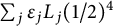
Finally, let us compare the proof of formula (1.6) (reciprocity formula in the holomorphic case) with the one given in [Reference Kuznetsov21, Reference Motohashi23] for Maass forms. It is well known that some convergence issues arise in the case of Maass forms. One way to avoid such problems is to apply the so-called “root number trick” by considering the moment
 $\sum _{j}\epsilon _jL_j(1/2)^4$
instead of
 $\sum _{j}L_j(1/2)^4$
. This is possible since
 $\epsilon _j=\pm 1$
and
 $L_j(1/2)=0$
if
 $\epsilon _j=-1$
. Note that this approach does not work when we consider the general shifted fourth moment. Another method that can be applied for arbitrary shifts (see [Reference Motohashi23]) is an application of a regularized Kuznetsov trace formula. However, it seems that these two methods are not applicable in the holomorphic case, where the same difficulties with convergence arise. Therefore, in our situation, the crucial idea, which allows to avoid all convergence issues, is the smooth decomposition (1.14) proposed by Kuznetsov.
2 Notation and preliminaries
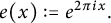
Let
 $e(x):=e^{2\pi ix}.$
Consider the number of divisors functions:
 $$ \begin{align} \sigma_v(n):=\sum_{d|n}d^v \end{align} $$
and
 $$ \begin{align} \tau_v(n):=\sum_{n_1n_2=n}\left( \frac{n_1}{n_2}\right)^v=n^{-v}\sigma_{2v}(n). \end{align} $$
The Riemann zeta function
 $\zeta (s)$
satisfies the functional equation
 $$ \begin{align} \zeta(s)=\mathcal{D}(s)\zeta(1-s),\quad \mathcal{D}(s)=2(2\pi)^{s-1}\Gamma(1-s)\sin\frac{\pi s}{2}. \end{align} $$
The Ramanujan identity is given by
 $$ \begin{align} \sum_{n=1}^{\infty}\frac{\sigma_a(n)\sigma_b(n)}{n^s}=\frac{\zeta(s)\zeta(s-a)\zeta(s-b)\zeta(s-a-b)}{\zeta(2s-a-b)}. \end{align} $$
Throughout the article,
 $H_{2k}$
denotes the Hecke normalized basis of the space of holomorphic cusp forms of weight
 $2k \geq 2$
and level one. For
 $f\in H_{2k}$
, the following Fourier expansion exists:
 $$ \begin{align} f(z)=\sum_{n\geq 1}\lambda_{f}(n)n^{k-1/2}\exp(2\pi inz), \quad \lambda_{f}(1)=1. \end{align} $$
Throughout the article,
 $B_{d}$
denotes the orthonormal basis
 $\{u_j\}$
of the space of Maass cusp forms of level one. We assume that any
 $u_j\in B_d$
is an eigenfunction of all Hecke operators and the hyperbolic Laplacian and denote by
 $\{\lambda _{j}(n)\}$
the eigenvalues of Hecke operators acting on
 $u_{j}$
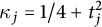
. Also
 $\kappa _{j}=1/4+t_{j}^2$
stands for (with
 $t_j>0$
) the eigenvalues of the hyperbolic Laplacian acting on
 $u_{j}$
. Finally, one has
 $$ \begin{align*} u_{j}(-\bar{z})=\varepsilon_j u_{j}(z),\quad \varepsilon_j=\pm1. \end{align*} $$
We call
 $u_j$
even or odd if
 $\varepsilon _j=1$
or
 $\varepsilon _j=-1$
, respectfully. It is known that
 $$ \begin{align*} u_{j}(x+iy)=\sqrt{y}\sum_{n\neq 0}\rho_{j}(n)K_{it_j}(2\pi|n|y)e(nx), \end{align*} $$
where
 $K_{\mu }(x)$
is the K-Bessel function and
 $\rho _{j}(n)=\rho _{j}(1)\lambda _{j}(n).$
Both
 $\lambda _{f}(n)$
and
 $\lambda _{j}(n)$
satisfy the following multiplicity relation:
 $$ \begin{align} \lambda(m)\lambda(n)=\sum_{d|(m,n)}\lambda\left( \frac{mn}{d^2}\right). \end{align} $$
For each
 $f\in H_{2k}$
and
 $u_j\in B_d$
, we define the associated L-functions as
 $$ \begin{align} L_f(s):=\sum_{n=1}^{\infty}\frac{\lambda_f(n)}{n^s},\quad L_j(s):=\sum_{n=1}^{\infty}\frac{\lambda_j(n)}{n^s}, \quad \Re{s}>1. \end{align} $$
It follows from (2.6) and (2.1) that
 $$ \begin{align} L_f(1/2+\alpha)L_f(1/2+\beta)=\zeta(1+\alpha+\beta) \sum_{n=1}^{\infty}\frac{\lambda_f(n)\sigma_{\alpha-\beta}(n)}{n^{1/2+\alpha}}, \end{align} $$
and the same holds for
 $L_j(s)$
.
Let
 $$ \begin{align} \omega_{j}:=\frac{|\rho_{j}(1)|^2}{\cosh{\pi t_j}} \end{align} $$
be the standard normalizing coefficient for Maass cusp forms and
 $$ \begin{align} \omega_f:=\frac{ \Gamma(2k-1)}{(4\pi )^{2k-1}\langle f,f\rangle_1} \end{align} $$
be the so-called harmonic weight (see [Reference Iwaniec, Luo and Sarnak16, Lemma 2.5]), where
 $\langle f,f\rangle _1$
is the Petersson inner product on the space
 $H_{2k}$
.
We will frequently use the Stirling bound [Reference Olver, Lozier, Boisvert and Clarke25, 5.11.9] for the Gamma function:
 $$ \begin{align} |\Gamma(x+iy)|\ll|y|^{x-1/2}e^{-\pi|y|/2}. \end{align} $$
It follows from the Stirling formula [Reference Olver, Lozier, Boisvert and Clarke25, 5.11.3, 5.11.13] that, for a bounded
 $|\alpha |$
, the following formula holds:
 $$ \begin{align} X_{k}(\alpha)=\frac{(2\pi)^{2\alpha}}{k^{2\alpha}}\left(1+O\left(\frac{1}{k}\right)\right). \end{align} $$
Lemma 2.1 For
 $\Re {d}<0$
and
 $-1<\Re {c}<-1-\Re {d}$
, one has
 $$ \begin{align} \int_0^{\infty}x^c(1+x)^ddx=\frac{\Gamma(c+1)\Gamma(-1-c-d)}{\Gamma(-d)}. \end{align} $$
Proof Equation (2.13) follows from [Reference Olver, Lozier, Boisvert and Clarke25, 5.12.3].
Let
 ${}_p\mathrm {I}_q$
denote the generalized hypergeometric function multiplied by suitable Gamma factors:

When
 $p=2,q=1,$
we will use the simplified notation
 ${}_2\mathrm {I}_1 (a_1,a_2,b_1;x)$
. Note that

In order to find an asymptotic expansion for the integrals of the form
 $$ \begin{align} I=\int_a^{b}g(x)e(f(x))dx, \end{align} $$
we will use the following version of the saddle point method due to Huxley [Reference Huxley14]. Recall that the saddle point is a solution of the equation
 $f'(x)=0$
.
Lemma 2.2 Let
 $f(x)$
and
 $g(x)$
be some smooth functions defined on the interval
 $[a,b]$
such that
 $g(a)=g(b)=0$
and
 $$ \begin{align} f^{(i)}(x)\ll\frac{\Theta_f}{\Omega_f^i},\quad g^{(j)}(x)\ll\frac{1}{\Omega_g^j},\quad f^{(2)}(x)\gg\frac{\Theta_f}{\Omega_f^2} \end{align} $$
for
 $i=1,2,3,4$
and
 $j=0,1,2$
. Suppose that
 $f'(x_0)=0$
for
 $a<x_0<b$
, and that
 $f(x)$
changes its sign from negative to positive at
 $x=x_0$
. Let
 $\kappa =\min (x_0-a,b-x_0)$
. Then,
 $$ \begin{align} I=\frac{g(x_0)e(f(x_0)+1/8)}{\sqrt{f"(x_0)}}+O\left(\frac{\Omega_f^4}{\kappa^3\Theta_f^2}+ \frac{\Omega_f}{\Theta_f^{3/2}}+\frac{\Omega_f^3}{\Theta_f^{3/2}\Omega_g^2}\right). \end{align} $$
3 Convolution formula for the second moment
As mentioned in the introduction, our method of investigating the fourth moment relies on the exact formula for the twisted second moment. Such formulas were proved independently by Kuznetsov (in his preprint from 1994 in Russian) and by Iwaniec–Sarnak (see [Reference Iwaniec and Sarnak17, Theorem 17]).
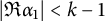
Theorem 3.1 For
 $|\Re {\alpha _1}|<k-1$
,
 $|\Re {\alpha _2}|<k-1,$
we have
 $$ \begin{align} \mathcal{M}_2(l;\alpha_1,\alpha_2) &:=\sum_{f \in H_{2k}}\omega_f\lambda_f(l)L_f(1/2+\alpha_1)L_f(1/2+\alpha_2) \nonumber\\ & =\mathcal{MT}_2(l;\alpha_1,\alpha_2)+\sum_{i=1}^3\mathcal{ET}^{(i)}_2(l;\alpha_1,\alpha_2), \end{align} $$
where
 $$ \begin{align} \mathcal{MT}_2(l;\alpha_1,\alpha_2) &:= \frac{\sigma_{\alpha_1-\alpha_2}(l)}{l^{1/2+\alpha_1}}\zeta(1+\alpha_1+\alpha_2)+ (-1)^kX_k(\alpha_1)\frac{\sigma_{\alpha_1+\alpha_2}(l)}{l^{1/2+\alpha_2}}\zeta(1-\alpha_1+\alpha_2) \nonumber\\ & \quad + (-1)^kX_k(\alpha_2)\frac{\sigma_{\alpha_1+\alpha_2}(l)}{l^{1/2+\alpha_1}}\zeta(1+\alpha_1-\alpha_2) \nonumber\\ & \quad + \frac{\sigma_{\alpha_1-\alpha_2}(l)}{l^{1/2-\alpha_2}}\zeta(1-\alpha_1-\alpha_2)X_k(\alpha_1)X_k(\alpha_2), \end{align} $$
 $$ \begin{align} \mathcal{ET}^{(1)}_2(l;\alpha_1,\alpha_2):=\frac{(-1)^k}{\sqrt{l}}\sum_{1 \leq n \leq l-1} \frac{\sigma_{\alpha_1-\alpha_2}(n)\sigma_{\alpha_1+\alpha_2}(l-n)}{n^{(\alpha_1-\alpha_2)/2}(l-n)^{(\alpha_1+\alpha_2)/2}} \phi_k\left(\frac{n}{l};\alpha_1,\alpha_2\right), \end{align} $$
 $$ \begin{align} \mathcal{ET}^{(2)}_2(l;\alpha_1,\alpha_2):=\frac{1}{\sqrt{l}}\sum_{n=1}^{\infty} \frac{\sigma_{\alpha_1+\alpha_2}(n)\sigma_{\alpha_1-\alpha_2}(n+l)}{n^{(\alpha_1+\alpha_2)/2}(n+l)^{(\alpha_1-\alpha_2)/2}} \Phi_k\left(\frac{l}{n+l};\alpha_1,\alpha_2\right), \end{align} $$
 $$ \begin{align} \mathcal{ET}^{(3)}_2(l;\alpha_1,\alpha_2):=(-1)^kX_k(\alpha_2)\mathcal{ET}^{(2)}_2(l;\alpha_1,-\alpha_2), \end{align} $$
and the weight functions are defined as
 $$ \begin{align} \phi_k(x;\alpha_1,\alpha_2):=\tilde{\phi}_k(x;\alpha_1,\alpha_2)+\tilde{\phi}_k(x;\alpha_2,\alpha_1), \end{align} $$
 $$ \begin{align} \tilde{\phi}_k(x;\alpha_1,\alpha_2) & :=\frac{(2\pi)^{1+\alpha_1+\alpha_2}}{2\sin{\pi\frac{\alpha_1-\alpha_2}{2}}} \frac{\Gamma(k-\alpha_1)}{\Gamma(1-\alpha_1+\alpha_2)\Gamma(k+\alpha_1)} x^{(\alpha_2-\alpha_1)/2}(1-x)^{-(\alpha_1+\alpha_2)/2} \nonumber\\ &\quad \times {}_2F_1 (k-\alpha_1,1-k-\alpha_1,1-\alpha_1+\alpha_2;x), \end{align} $$
 $$ \begin{align} \Phi_k(x;\alpha_1,\alpha_2) & :=2(2\pi)^{\alpha_1+\alpha_2} \cos{\pi\frac{\alpha_1+\alpha_2}{2}}x^k(1-x)^{-(\alpha_1+\alpha_2)/2} \nonumber\\ & \quad \times {}_2\mathrm{I}_1 (k-\alpha_1,k-\alpha_2,2k;x). \end{align} $$
Proof The proof of the theorem formulated in slightly different notations can be found in [Reference Balkanova and Frolenkov4, Theorem 4.2]. To obtain the stated version, one needs to take
 $u=(\alpha _1+\alpha _2)/2$
and
 $v=(\alpha _1-\alpha _2)/2$
in [Reference Balkanova and Frolenkov4, Theorem 4.2] and to use the relation (2.2). After that, it is left to prove a new relation (3.5). It follows from [Reference Balkanova and Frolenkov4, (4.6), (4.10)] that
 $$ \begin{align} \mathcal{ET}^{(3)}_2(l;\alpha_1,\alpha_2)= \frac{(-1)^k}{\sqrt{l}}\sum_{n=1}^{\infty} \frac{\sigma_{\alpha_1-\alpha_2}(n)\sigma_{\alpha_1+\alpha_2}(n+l)}{n^{(\alpha_1-\alpha_2)/2}(n+l)^{(\alpha_1+\alpha_2)/2}} \psi_k\left(\frac{l}{n};\alpha_1,\alpha_2\right), \end{align} $$
where
 $$ \begin{align} \psi_k(x;\alpha_1,\alpha_2) &=2(2\pi)^{\alpha_1+\alpha_2} \cos{\pi\frac{\alpha_1-\alpha_2}{2}}x^k(1+x)^{-(\alpha_1+\alpha_2)/2} \nonumber\\ & \quad \times {}_2\mathrm{I}_1 (k-\alpha_2,k-\alpha_1,2k;-x). \end{align} $$
Applying [Reference Olver, Lozier, Boisvert and Clarke25, 15.8.1], we find that
 $$ \begin{align} \psi_k(x;\alpha_1,\alpha_2)& = 2(2\pi)^{\alpha_1+\alpha_2} \cos{\pi\frac{\alpha_1-\alpha_2}{2}}\frac{\Gamma(k-\alpha_2)}{\Gamma(k+\alpha_2)} \left(\frac{x}{1+x}\right)^k(1+x)^{(\alpha_1-\alpha_2)/2} \nonumber\\ & \quad\times {}_2\mathrm{I}_1 \left(k-\alpha_1,k+\alpha_2,2k;\frac{x}{1+x}\right) \nonumber\\ & = (2\pi)^{2\alpha_2}\frac{\Gamma(k-\alpha_2)}{\Gamma(k+\alpha_2)}\Phi_k\left(\frac{x}{1+x};\alpha_1,-\alpha_2\right). \end{align} $$
4 Special functions
In this section, we collect various results on special functions that will be used later in the proof of the main theorem.
Lemma 4.1 For
 $0<x<1,$
the following identity holds:
 $$ \begin{align} \phi_k(1-x;\alpha_1,\alpha_2)=(-1)^kX_k(\alpha_2)\phi_k(x;\alpha_1,-\alpha_2). \end{align} $$
Proof According to [Reference Beitman and Erdelyi6, (33), p. 107], one has
 $$ \begin{align} & {}_2F_1 (k-\alpha_1,1-k-\alpha_1,1-\alpha_1+\alpha_2;x)\nonumber\\ &\quad = \frac{\Gamma(1-\alpha_1+\alpha_2)\Gamma(\alpha_1+\alpha_2)}{\Gamma(1-k+\alpha_2)\Gamma(k+\alpha_2)}{}_2F_1 (k-\alpha_1,1-k-\alpha_1,1-\alpha_1-\alpha_2;1-x) \nonumber\\ & \qquad + \frac{\Gamma(1-\alpha_1+\alpha_2)\Gamma(-\alpha_1-\alpha_2)}{\Gamma(1-k-\alpha_1)\Gamma(k-\alpha_1)}(1-x)^{\alpha_1+\alpha_2} \nonumber\\ &\qquad \times {}_2F_1 (k+\alpha_2,1-k+\alpha_2,1+\alpha_1+\alpha_2;1-x). \end{align} $$
Making the change
 $\alpha _1\leftrightarrow \alpha _2$
in (4.2) and applying to each of the hypergeometric functions, the following relation (see [Reference Olver, Lozier, Boisvert and Clarke25, 15.8.1]):
 $$ \begin{align} {}_2F_1 (a,b,c;1-x)=x^{c-a-b}{}_2F_1 (c-a,c-b,c;1-x), \end{align} $$
we obtain
 $$ \begin{align} & {}_2F_1 (k-\alpha_2,1-k-\alpha_2,1-\alpha_2+\alpha_1;x) \nonumber\\ &\quad = \frac{\Gamma(1-\alpha_2+\alpha_1)\Gamma(\alpha_1+\alpha_2)}{\Gamma(1-k+\alpha_1)\Gamma(k+\alpha_1)}x^{\alpha_2-\alpha_1} {}_2F_1 (k-\alpha_1,1-k-\alpha_1,1-\alpha_1-\alpha_2;1-x) \nonumber\\ & \qquad + \frac{\Gamma(1-\alpha_2+\alpha_1)\Gamma(-\alpha_1-\alpha_2)}{\Gamma(1-k-\alpha_2)\Gamma(k-\alpha_2)}(1-x)^{\alpha_1+\alpha_2}x^{\alpha_2-\alpha_1} \nonumber\\ &\qquad \times {}_2F_1 (k+\alpha_2,1-k+\alpha_2,1+\alpha_1+\alpha_2;1-x). \end{align} $$
Using (3.6), (3.7), (4.2), (4.4) and the relations
 $$ \begin{align} &\frac{\Gamma(k-\alpha_1)}{\Gamma(1-k+\alpha_2)}-\frac{\Gamma(k-\alpha_2)}{\Gamma(1-k+\alpha_1)} \nonumber\\ &\quad = \frac{2(-1)^k}{\pi}\Gamma(k-\alpha_1)\Gamma(k-\alpha_2)\sin\pi\frac{\alpha_1-\alpha_2}{2}\cos\pi\frac{\alpha_1+\alpha_2}{2}, \end{align} $$
 $$ \begin{align} & \frac{1}{\Gamma(k+\alpha_1)\Gamma(1-k-\alpha_1)}- \frac{1}{\Gamma(k+\alpha_2)\Gamma(1-k-\alpha_2)} \nonumber\\ &\quad = \frac{2(-1)^k}{\pi}\sin\pi\frac{\alpha_1-\alpha_2}{2}\cos\pi\frac{\alpha_1+\alpha_2}{2}, \end{align} $$
which follow from [Reference Olver, Lozier, Boisvert and Clarke25, 5.5.3], we show that
 $$ \begin{align} \phi_k(x;\alpha_1,\alpha_2) &= \frac{(-1)^k}{\pi}\cos\pi\frac{\alpha_1+\alpha_2}{2}\Gamma(\alpha_1+\alpha_2) (2\pi)^{1+\alpha_1+\alpha_2}x^{(\alpha_2-\alpha_1)/2}(1-x)^{-(\alpha_1+\alpha_2)/2} \nonumber\\ & \quad \times \frac{\Gamma(k-\alpha_1)\Gamma(k-\alpha_2)}{\Gamma(k+\alpha_1)\Gamma(k+\alpha_2)} {}_2F_1 (k-\alpha_1,1-k-\alpha_1,1-\alpha_1-\alpha_2;1-x) \nonumber\\ & \quad + \frac{(-1)^k}{\pi}\cos\pi\frac{\alpha_1+\alpha_2}{2}\Gamma(-\alpha_1-\alpha_2) (2\pi)^{1+\alpha_1+\alpha_2} \nonumber\\ &\quad \times x^{(\alpha_2-\alpha_1)/2}(1-x)^{(\alpha_1+\alpha_2)/2}{}_2F_1 (k+\alpha_2,1-k+\alpha_2,1+\alpha_1+\alpha_2;1-x). \end{align} $$
Applying [Reference Olver, Lozier, Boisvert and Clarke25, 5.5.3], we infer that
 $$ \begin{align} \frac{\Gamma(\alpha_1+\alpha_2)}{\pi}\cos\pi\frac{\alpha_1+\alpha_2}{2}= \frac{1}{2\sin\pi\frac{\alpha_1+\alpha_2}{2}\Gamma(1-\alpha_1-\alpha_2)}, \end{align} $$
 $$ \begin{align} \frac{\Gamma(-\alpha_1-\alpha_2)}{\pi}\cos\pi\frac{\alpha_1+\alpha_2}{2}= \frac{1}{2\sin\pi\frac{-\alpha_1-\alpha_2}{2}\Gamma(1+\alpha_1+\alpha_2)}. \end{align} $$
Substituting (4.8) and (4.9) to (4.7) and using (3.6) and (3.7), we finally prove that
 $$ \begin{align} \phi_k(x;\alpha_1,\alpha_2)=(-1)^kX_k(\alpha_2)\phi_k(1-x;\alpha_1,-\alpha_2). \end{align} $$
Let
 $$ \begin{align} \Gamma(k,\alpha_1,\alpha_2;s):= \frac{\Gamma(k-1/2+s/2)}{\Gamma(k+1/2-s/2)}\Gamma(1/2-\alpha_1-s/2)\Gamma(1/2-\alpha_2-s/2), \end{align} $$
 $$ \begin{align} J_s(k,\alpha_1,\alpha_2;x):=\frac{1}{2\pi i}\int_{(\sigma)}\Gamma(k,\alpha_1,\alpha_2;s)\sin\left(\pi\frac{s+\alpha_1+\alpha_2}{2}\right)x^{s/2}ds, \end{align} $$
where
 $1-2k<\sigma <1-2\max (|\Re {\alpha _1}|,|\Re {\alpha _2}|)$
. The next lemma is proven in [Reference Frolenkov10, Lemma 2.2].
Lemma 4.2 For
 $0<x<1$
and
 $\Re {(\alpha _1+\alpha _2)}>0$
,
 $|\Re {\alpha _1}|<k$
,
 $|\Re {\alpha _2}|<k,$
 $$ \begin{align} \phi_k(x;\alpha_1,\alpha_2)=(2\pi)^{\alpha_1+\alpha_2}x^{-1/2+\alpha_1/2+\alpha_2/2}(1-x)^{-\alpha_1/2-\alpha_2/2}J_s(k,\alpha_1,\alpha_2;x), \end{align} $$
 $$ \begin{align} \Phi_k(x;\alpha_1,\alpha_2)=(-1)^k(2\pi)^{\alpha_1+\alpha_2}x^{1/2}(1-x)^{-\alpha_1/2-\alpha_2/2}J_s(k,\alpha_1,\alpha_2;1/x). \end{align} $$
Lemma 4.3 The following asymptotic formulas hold:
 $$ \begin{align} \phi_k(x;\alpha_1,\alpha_2)\kern1.4pt{\sim}\kern1.4pt x^{-|\Re{(\alpha_1-\alpha_2)}|/2}\text{ as } x\rightarrow0,\quad\! \phi_k(x;\alpha_1,\alpha_2)\kern1.4pt{\sim}\kern1.4pt(1-x)^{-|\Re{(\alpha_1+\alpha_2)}|/2}\text{ as } x\kern1.4pt{\rightarrow}\kern1.4pt1, \end{align} $$
 $$ \begin{align} \Phi_k\left(x;\alpha_1,\alpha_2\right)\sim x^k\text{ as } x\rightarrow0,\quad \Phi_k\left(x;\alpha_1,\alpha_2\right)\sim(1-x)^{-|\Re{(\alpha_1+\alpha_2)}|/2}\text{ as } x\rightarrow1. \end{align} $$
Proof In case when
 $x\rightarrow 1$
, the formula (4.15) follows from (3.6) and (3.7) after using [Reference Olver, Lozier, Boisvert and Clarke25, 15.4.20, 15.4.23].
In case when
 $x\rightarrow 0$
, the formula (4.15) follows from the series representation for the hypergeometric function. One can prove (4.16) in a similar way.
Lemma 4.4 For
 $0<x<1,$
the function
 $$ \begin{align} Y(x;\alpha_1,\alpha_2):=\sqrt{x(1-x)}\tilde{\phi}_k(x;\alpha_1,\alpha_2) \end{align} $$
is a solution of the differential equation
 $$ \begin{align} Y"(x)+\mathcal{I}(x;\alpha_1,\alpha_2)Y(x)=0, \end{align} $$
where
 $$ \begin{align} \mathcal{I}(x;\alpha_1,\alpha_2)& = \frac{(2k-1)^2}{4x(1-x)}+ \frac{1-(\alpha_2-\alpha_1)^2}{4x^2}+ \frac{1-(\alpha_2+\alpha_1)^2}{4(1-x)^2} \nonumber\\ &\quad + \frac{1-(\alpha_2-\alpha_1)^2-(\alpha_2+\alpha_1)^2}{4x(1-x)}. \end{align} $$
Proof This is a generalization of [Reference Balkanova and Frolenkov4, Corollary 5.6] (see also [Reference Beitman and Erdelyi6, Section 2.7.2, (8), (9)]).
Lemma 4.5 Let
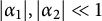 $|\alpha _1|,|\alpha _2|\ll 1$
. For
 $0<x\ll k^{-2+\epsilon }$
, one has
 $$ \begin{align} \tilde{\phi}_k(x;\alpha_1,\alpha_2)\ll k^{-2\Re{\alpha_1}} x^{(\Re{\alpha_2}-\Re{\alpha_1})/2}. \end{align} $$
For
 $k^{-2+\epsilon }\ll x<1-\delta $
, one has
 $$ \begin{align} \tilde{\phi}_k(x;\alpha_1,\alpha_2)\ll \frac{1}{k^{1/2+\Re{\alpha_2}+\Re{\alpha_1}}x^{1/4}}. \end{align} $$
Proof It follows from [Reference Balkanova, Conrey and Frolenkov1, Lemmas 3.10 and 3.12, (3.56)] that for
 $0<x\ll k^{-2+\epsilon }$
, one has
 $$ \begin{align} {}_2F_1 (k-\alpha_1,1-k-\alpha_1,1-\alpha_1+\alpha_2;x)\ll1, \end{align} $$
and for
 $k^{-2+\epsilon }\ll x<\delta ,$
 $$ \begin{align} {}_2F_1 (k-\alpha_1,1-k-\alpha_1,1-\alpha_1+\alpha_2;x) &\ll \frac{1}{(k\arccos\sqrt{1-2x})^{1/2+\Re{\alpha_2}-\Re{\alpha_1}}} \nonumber\\ & \ll \frac{1}{(k\sqrt{x})^{1/2+\Re{\alpha_2}-\Re{\alpha_1}}}. \end{align} $$
For
 $\delta <x<1-\delta ,$
the estimate (4.23) follows from [Reference Balkanova, Conrey and Frolenkov1, Lemma 3.9]. Finally, using (3.7), we prove the lemma.
Similar estimates are also valid when
 $\alpha _1=\alpha _2=0$
. The following result is a consequence of [Reference Balkanova and Frolenkov4, Theorems 5.10 and 5.14].
Lemma 4.6 The following estimates hold:
 $$ \begin{align} \phi_k(x)\ll\begin{cases} \log(k\sqrt{x}),\quad 0<x\ll k^{-2+\epsilon};\\ \log(k\sqrt{1-x}),\quad 1-k^{-2+\epsilon}<x<1;\\ k^{-1/2}x^{-1/4},\quad k^{-2+\epsilon}\ll x<1/2;\\ k^{-1/2}(1-x)^{-1/4},\quad 1/2<x<1-k^{-2+\epsilon}. \end{cases} \end{align} $$
Lemma 4.7 Let
 $u=k-1/2$
. Then, for
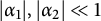 $|\alpha _1|,|\alpha _2|\ll 1$
,
 $\xi>0,$
and
 $k\rightarrow +\infty ,$
one has
 $$ \begin{align} \Phi_k\left(\frac{1}{\cosh^2{\left(\sqrt{\xi}/2\right)}};\alpha_1,\alpha_2\right)\left( \xi\sinh^2{\left(\sqrt{\xi}\right)}\right)^{1/4} \ll \frac{\sqrt{\xi}}{k^{\alpha_1+\alpha_2}}K_{\alpha_1+\alpha_2}(u\sqrt{\xi}). \end{align} $$
Proof As in the proof of Lemma 4.5 (see also [Reference Balkanova, Conrey and Frolenkov1, Lemmas 3.10 and 3.12]), one may try to refer to the results in [Reference Farid Khwaja and Olde Daalhuis9]. Now, we briefly explain the difficulties arising on this way. First, one needs to transform the hypergeometric function in (3.8) to the one of the form treated in [Reference Farid Khwaja and Olde Daalhuis9, Tables 1 and 3]. A possible way to do this is to apply [Reference Beitman and Erdelyi6, Section 2.9, (7), (23), (33)], which results in a combination of the functions
 $$ \begin{align} {}_2F_1 (k\pm\alpha_1,1-k\pm\alpha_1,1\pm\alpha_1\pm\alpha_2;1-x^{-1}). \end{align} $$
An asymptotic formula for (4.26) in terms of the I-Bessel functions is provided by [Reference Farid Khwaja and Olde Daalhuis9, Theorem 3.1]. It turns out that (4.26) grows exponentially, while
 $\Phi _k(x,\alpha _1,\alpha _2)$
should decay exponentially. This means that there is a massive cancellation between functions (4.26) in their linear combination representing
 $\Phi _k$
. This makes impossible to apply the results of [Reference Farid Khwaja and Olde Daalhuis9]. Therefore, we are going to adapt the results of [Reference Balkanova and Frolenkov4, Section 5.3]. As in [Reference Balkanova and Frolenkov4, Lemma 5.15], the function
 $$ \begin{align} y(x;\alpha_1,\alpha_2):=\Phi_k\left(x;\alpha_1,\alpha_2\right)\sqrt{1-x} \end{align} $$
satisfies the differential equation
 $$ \begin{align} y"(x)-(u^2f(x)+g(x))y(x)=0, \end{align} $$
 $$ \begin{align} f(x):=\frac{1}{x^2(1-x)}, \quad g(x):=-\frac{1}{4x^2}-\frac{1-(\alpha_1+\alpha_2)^2}{4(1-x)^2}-\frac{1-4\alpha_1\alpha_2}{4x(1-x)}. \end{align} $$
Note that the function
 $f(x)$
coincides with the one in [Reference Balkanova and Frolenkov4, (5.65)] and the function
 $g(x)$
differs slightly. Making the same change of variable as in [Reference Balkanova and Frolenkov4, (5.70)]:
 $$ \begin{align} \xi:=4 \operatorname{\mathrm{artanh}}^2{(\sqrt{1-x})}, \end{align} $$
we obtain that the function (see [Reference Balkanova and Frolenkov4, (5.69)])
 $$ \begin{align} Z(x):=\frac{y(x)}{\alpha(x)}, \quad \alpha(x):=\frac{(x^2-x^3)^{1/4}}{2(\operatorname{\mathrm{artanh}}{(\sqrt{1-x})})^{1/2}} \end{align} $$
satisfies
 $$ \begin{align} \frac{d^2Z}{d\xi^2}+\left[ -\frac{u^2}{4\xi}+\frac{1}{4\xi^2}-\frac{\psi(\xi)}{\xi}\right]Z=0, \end{align} $$
where
 $$ \begin{align} \psi(\xi)=\frac{1}{16}\left(\frac{1}{\xi}-\frac{1-4(\alpha_1+\alpha_2)^2}{\sinh^2{(\sqrt{\xi})}}+\frac{4\alpha_1\alpha_2}{\cosh^2{(\sqrt{\xi}/2)}} \right). \end{align} $$
The function (4.33) is only slightly different from [Reference Balkanova and Frolenkov4, (5.68)], however is no more analytic at
 $\xi =0$
. To overcome this difficulty, we change the form of an approximating differential equation from [Reference Balkanova and Frolenkov4, (5.71)] to
 $$ \begin{align} Z"+\left(-\frac{u^2}{4\xi}+\frac{1-(\alpha_1+\alpha_2)^2}{4\xi^2} \right)Z=0. \end{align} $$
So we rewrite (4.32) and (4.33) in the form
 $$ \begin{align} \frac{d^2Z}{d\xi^2}+\left[ -\frac{u^2}{4\xi}+\frac{1-(\alpha_1+\alpha_2)^2}{4\xi^2}-\frac{\psi(\xi)}{\xi}\right]Z=0, \end{align} $$
where
 $$ \begin{align} \psi(\xi)=\frac{1-4(\alpha_1+\alpha_2)^2}{16}\left(\frac{1}{\xi}-\frac{1}{\sinh^2{(\sqrt{\xi})}}\right)+\frac{\alpha_1\alpha_2}{4\cosh^2{(\sqrt{\xi}/2)}}. \end{align} $$
Now, the function
 $\psi (\xi )$
is analytic at
 $\xi =0$
, and we can perform all computations in the same way as in [Reference Balkanova and Frolenkov4, Section 5.3]. Solutions of (4.34) are given by (see [Reference Olver, Lozier, Boisvert and Clarke25, Section 10.36, Equation (10.13.2)]):
 $$ \begin{align} Z_L=\sqrt{\xi}L_{\alpha_1+\alpha_2}(u\sqrt{\xi}), \end{align} $$
where
 $$ \begin{align} L_v(x):=\begin{cases} I_v(x)\\e^{\pi i v}K_v(x). \end{cases} \end{align} $$
Arguing in the same way as in [Reference Balkanova and Frolenkov4, Theorem 5.16] and using the analog of [Reference Balkanova and Frolenkov4, (5.92), (5.93)], we obtain
 $$ \begin{align} \Phi_k\left(\frac{1}{\cosh^2{\left(\sqrt{\xi}/2\right)}} \right)\left( \xi\sinh^2{\left(\sqrt{\xi}\right)}\right)^{1/4}= C_KZ_K(\xi), \end{align} $$
where
 $$ \begin{align} C_K=2\frac{\Gamma(k-\alpha_1)\Gamma(k-\alpha_2)}{\Gamma(2k)}\frac{2^{2k}\sqrt{u}}{\sqrt{\pi}}\frac{(2\pi)^{\alpha_1+\alpha_2}\cos\pi\frac{\alpha_1+\alpha_2}{2}}{e^{\pi i(\alpha_1+\alpha_2)}}\left(1+O\left(\frac{1}{u}\right)\right)\ll\frac{1}{k^{\Re{\alpha_1}+\Re{\alpha_2}}}, \end{align} $$
and
 $Z_K(\xi )$
is the same as in [Reference Balkanova and Frolenkov4, (5.86)] with
 $K_0(x)$
,
 $K_1(x)$
replaced by
 $K_{\alpha _1+\alpha _2}(x), K_{1+\alpha _1+\alpha _2}(x)$
, respectively. Note that the coefficients
 $A_K(n;\xi )$
,
 $B_K(n;\xi )$
now also depend on
 $\alpha _1,\alpha _2$
, but if
 $|\alpha _1|,|\alpha _2|<\epsilon $
, then they are still uniformly bounded by some constant. It follows from the structure of
 $Z_K(\xi )$
that it is bounded by
 $\sqrt {\xi }K_{\alpha _1+\alpha _2}(u\sqrt {\xi })$
. This completes the proof of (4.25).
Applying (4.25) and [Reference Olver, Lozier, Boisvert and Clarke25, 10.25.3, 10.30.3], we prove the following estimate.
Corollary 4.8 For
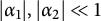 $|\alpha _1|,|\alpha _2|\ll 1$
and
 $x\gg k^{-2+\epsilon }$
, one has
 $$ \begin{align} \Phi_k\left(\frac{1}{1+x};\alpha_1,\alpha_2\right)\ll \frac{e^{-(2k-1)\log(\sqrt{1+x}+\sqrt{x})}}{(1+x)^{1/4}x^{1/4}k^{1/2+\Re{\alpha_1}+\Re{\alpha_2}}}. \end{align} $$
If
 $\alpha _1=\alpha _2=0,$
then one has
 $$ \begin{align} \Phi_k\left(x\right)\ll \frac{x^{1/2}e^{-(2k-1)\log((1+\sqrt{1-x})/\sqrt{x})}}{(1-x)^{1/4}k^{1/2}} \quad \text{ for } x<1-k^{-2+\epsilon} \end{align} $$
and
 $$ \begin{align} \Phi_k\left(x\right)\ll\log(k\sqrt{1-x})\quad \text{ for }1-k^{-2+\epsilon}<x<1. \end{align} $$
Now, we are going to obtain an asymptotic formula for the hypergeometric function that will arise in the additive divisor problem. This result is an analog of [Reference Zavorotny28, Lemma 2.4].
Lemma 4.9 For
 $|\alpha |,|\beta |\ll 1$
,
 $y>y_0>0,$
and
 $r\rightarrow +\infty ,$
one has
 $$ \begin{align} & {}_2F_1 \left(\frac{1+\alpha-\beta}{2}+ir,\frac{1-\alpha-\beta}{2}+ir,1+2ir;\frac{-1}{y}\right) \nonumber\\ &\qquad =\frac{(4y)^{ir}y^{1/4-\alpha+\beta/2}}{(\sqrt{1+y}+\sqrt{y})^{2ir}(1+y)^{1/4-\alpha+\beta/2}}\left(1+\sum_{n=1}^N\frac{a_n(y)}{r^n}\right)+ O\left(\frac{1}{yr^{N+1}}\right), \end{align} $$
where
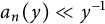 $a_n(y)\ll y^{-1}$
.
Proof Applying [Reference Olver, Lozier, Boisvert and Clarke25, 15.8.1], we obtain
 $$ \begin{align} & {}_2F_1 \left(\frac{1+\alpha-\beta}{2}+ir,\frac{1-\alpha-\beta}{2}+ir,1+2ir;\frac{-1}{y}\right) \nonumber\\ & \quad =\left(\frac{1+y}{y}\right)^{-1/2-\alpha/2+\beta/2-ir} {}_2F_1 \left(\frac{1+\alpha-\beta}{2}+ir,\frac{1+\alpha+\beta}{2}+ir,1+2ir;\frac{1}{1+y}\right).\nonumber\\ \end{align} $$
The function
 $$ \begin{align} y(x)=x^{1/2+ir}(1-x)^{1/2+\alpha/2}{}_2F_1 \left(\frac{1+\alpha-\beta}{2}+ir,\frac{1+\alpha+\beta}{2}+ir,1+2ir;x\right) \end{align} $$
satisfies [Reference Beitman and Erdelyi6, p. 96] the differential equation
 $$ \begin{align} y"(x)+H(x)y(x)=0, \end{align} $$
where
 $$ \begin{align} H(x)=\frac{r^2}{x^2(1-x)}+\frac{1}{4x^2}+\frac{1-\alpha^2}{4(1-x)^2}+\frac{1+\beta^2-\alpha^2}{4x(1-x)}. \end{align} $$
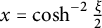
Arguing in the same way as in [Reference Balkanova and Frolenkov4, (5.20)–(5.23)] and choosing
 $\alpha (x)=x^{1/2}(1-x)^{1/4}$
(therefore, making the change of variables
 $x=\cosh ^{-2}\frac {\xi }{2}$
), we obtain that the function
 $$ \begin{align} U(\xi)=\frac{\tanh^{1/2+\alpha}(\xi/2)}{\cosh^{2ir}(\xi/2)} {}_2F_1 \left(\frac{1+\alpha-\beta}{2}+ir,\frac{1+\alpha+\beta}{2}+ir,1+2ir;\frac{1}{\cosh^2\frac{\xi}{2}}\right) \end{align} $$
satisfies
 $$ \begin{align*} U"(\xi)+\left( r^2+\frac{1-4\alpha^2}{4\sinh^2\xi}+\frac{\beta^2-\alpha^2}{4\cosh^2{\xi/2}}\right)U(\xi)=0. \end{align*} $$
Either arguing in the same way as in [Reference Zavorotny28, Lemma 2.4] or rather applying [Reference Olver24, Section 10.3, Theorem 3.1] and the discussions afterward, one can prove that
 $$ \begin{align} U(\xi)=2^{2ir}e^{-ir\xi}\left(1+\sum_{n=1}^N\frac{A_n(\xi)}{ir}\right)+O\left(\frac{1}{e^{\xi}r^{N+1}}\right). \end{align} $$
Now, (4.44) follows from (4.45), (4.49), and (4.50) after some straightforward computations.
Note that the result (4.44) could be obtained with the use of the saddle point method like in [Reference Jutila18, p. 173].
For the sake of simplicity, let us introduce some additional notation:
 $$ \begin{align} k_0(x,v):=\frac{1}{2\cos(\pi (1/2+v))}\left(J_{2v}(x)-J_{-2v}(x) \right), \end{align} $$
 $$ \begin{align} k_1(x,v):=\frac{2}{\pi}\sin(\pi(1/2+v))K_{2v}(x). \end{align} $$
According to [Reference Balkanova and Frolenkov4, Lemma 2.2], the following result holds.
Lemma 4.10 Let
 $$ \begin{align} \gamma(u,v):=\frac{2^{2u-1}}{\pi}\Gamma(u+v)\Gamma(u-v). \end{align} $$
For
 $3/2>Re{w}> 2|\Re {v}|$
, one has
 $$ \begin{align} \int_{0}^{\infty}k_0(x,v)x^{w-1}dx=\gamma(w/2,v)\cos{(\pi w/2)}, \end{align} $$
and for
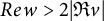 $Re{w}> 2|\Re {v}|$
, one has
 $$ \begin{align} \int_{0}^{\infty}k_1(x,v)x^{w-1}dx=\gamma(w/2,v)\sin{(\pi (1/2+v))}. \end{align} $$
Corollary 4.11 For
 $\Delta _0,\Delta _1> 2|\Re {v}|$
, the following formulas hold:
 $$ \begin{align} k_0(x,v)=\frac{1}{2\pi i}\int_{(\Delta_0)}\gamma(w/2,v)\cos{(\pi w/2)}x^{-w}dw, \end{align} $$
 $$ \begin{align} k_1(x,v)=\frac{1}{2\pi i}\int_{(\Delta_1)}\gamma(w/2,v)\sin{(\pi (1/2+v))}x^{-w}dw. \end{align} $$
For
 $\Delta _0,\Delta _1<\min (1,1+2\Re {v}),$
one has
 $$ \begin{align} k_0(x,v)=\frac{2^{2+2v}}{\pi x^{2+2v}}\frac{1}{2\pi i}\int_{(\Delta_0)}\Gamma(1-s) \Gamma(1+2v-s)\cos\pi(1+v-s)\frac{x^{2s}}{4^s}ds, \end{align} $$
 $$ \begin{align} k_1(x,v)=\frac{2^{2+2v}\sin{(\pi (1/2+v))}}{\pi x^{2+2v}}\frac{1}{2\pi i}\int_{(\Delta_1)}\Gamma(1-s) \Gamma(1+2v-s)\frac{x^{2s}}{4^s}ds. \end{align} $$
5 The binary additive divisor problem
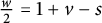
Following Motohashi’s book [Reference Motohashi22, p. 531], let
 $$ \begin{align} A(l,\alpha,\beta;W):=\sum_{n=1}^{\infty}\sigma_{\alpha}(n)\sigma_{\beta}(n+l)W\left(\frac{n}{l}\right). \end{align} $$
The problem of investigating the asymptotic behavior of (5.1) has a long history (see [Reference Balkanova and Frolenkov2] for references). It is shown in [Reference Balkanova and Frolenkov2] that the best known estimate on the reminder in the asymptotic formula for (5.1) can be obtained, among other methods, using the results of [Reference Motohashi22]. We will apply an exact formula for (5.1) proved by Motohashi [Reference Motohashi22] (a similar formula has also been obtained by Kuznetsov [Reference Kuznetsov20]).
Theorem 5.1 Assume that
 $-1-\Re {\beta }<\Re {\alpha }<1+\Re {\beta }$
. Let W be a sufficiently good function such that all the series and integrals below are absolutely convergent. Then,
 $$ \begin{align} A(l,\alpha,\beta;W)=U(l,\alpha,\beta;W)+E_{h}(l,\alpha,\beta;W)+E_{d}(l,\alpha,\beta;W)+E_{c}(l,\alpha,\beta;W), \end{align} $$
where
 $$ \begin{align} U(l,\alpha,\beta;W)=\int_0^{\infty}W(x)\mu(l,\alpha,\beta;x)dx, \end{align} $$
 $$ \begin{align} \mu(l,\alpha,\beta;x) & = \sigma_{1+\alpha+\beta}(l)\frac{\zeta(1+\alpha)\zeta(1+\beta)}{\zeta(2+\alpha+\beta)}x^{\alpha}(1+x)^{\beta} \nonumber\\ &\quad + l^{\alpha}\sigma_{1-\alpha+\beta}(l)\frac{\zeta(1-\alpha)\zeta(1+\beta)}{\zeta(2-\alpha+\beta)}(1+x)^{\beta} \nonumber\\ &\quad + l^{\beta}\sigma_{1+\alpha-\beta}(l)\frac{\zeta(1+\alpha)\zeta(1-\beta)}{\zeta(2+\alpha-\beta)}x^{\alpha}+ l^{\alpha+\beta}\sigma_{1-\alpha-\beta}(l)\frac{\zeta(1-\alpha)\zeta(1-\beta)}{\zeta(2-\alpha-\beta)}, \end{align} $$
 $$ \begin{align} E_{h}(l,\alpha,\beta;W) & = 2(2\pi)^{\beta-1}l^{(1+\alpha+\beta)/2} \sum_{m=6}^{\infty}\frac{2m-1}{\pi^2}\sum_{f\in H_{2m}} \omega_f\lambda_f(l)L_f\left(\frac{1+\alpha-\beta}{2}\right) \nonumber\\ & \quad\times L_f\left(\frac{1-\alpha-\beta}{2}\right)\widehat{W}(\alpha,\beta;m), \end{align} $$
 $$ \begin{align} E_{d}(l,\alpha,\beta;W) &=2(2\pi)^{\beta-1}l^{(1+\alpha+\beta)/2} \sum_{j} \omega_j\lambda_j(l)L_j\left(\frac{1+\alpha-\beta}{2}\right) \nonumber\\ &\quad \times L_j\left(\frac{1-\alpha-\beta}{2}\right) \left(\widehat{W}^{+}(\alpha,\beta;t_j)+\varepsilon_j\widehat{W}^{-}(\alpha,\beta;t_j)\right), \end{align} $$
 $$ \begin{align} E_{c}(l,\alpha,\beta;W) &=4(2\pi)^{\beta-1}l^{(1+\alpha+\beta)/2}\frac{1}{2\pi i} \int_{(0)} \frac{\sigma_{2\xi}(l)\mathcal{Z}_4(\alpha,\beta,\xi)}{l^{\xi}\zeta(1+2\xi)\zeta(1-2\xi)} \nonumber\\ &\quad \times \left(\widehat{W}^{+}(\alpha,\beta;-i\xi)+\widehat{W}^{-}(\alpha,\beta;-i\xi)\right)d\xi \end{align} $$
with
 $$ \begin{align} \mathcal{Z}_4(\alpha,\beta,\xi) &=\zeta\left(\frac{1-\alpha-\beta}{2}+\xi\right) \zeta\left(\frac{1+\alpha-\beta}{2}+\xi\right) \zeta \left(\frac{1-\alpha-\beta}{2}-\xi\right) \nonumber\\ &\quad \times \zeta\left(\frac{1+\alpha-\beta}{2}-\xi\right), \end{align} $$
 $$ \begin{align} \widehat{W}(\alpha,\beta;m)=\frac{\pi(-1)^m}{2}\cos\frac{\pi\alpha}{2}\int_0^{\infty}\frac{W(y)}{y^{m-\frac{\alpha+\beta}{2}}} {}_2\mathrm{I}_1 \left(m+\alpha-\frac{\beta}{2},m-\alpha-\frac{\beta}{2},2m;\frac{-1}{y}\right)dy, \end{align} $$
 $$ \begin{align} \widehat{W}^{+}(\alpha,\beta;r)= \frac{\pi i\cos\frac{\pi\alpha}{2}}{4\sinh(\pi r)}\widehat{W}^{0}(\alpha,\beta;ir)- \frac{\pi i\cos\frac{\pi\alpha}{2}}{4\sinh(\pi r)} \widehat{W}^{0}(\alpha,\beta;-ir), \end{align} $$
 $$ \begin{align} \widehat{W}^{-}(\alpha,\beta;r)= \frac{-\pi i\sin\pi(ir-\beta/2)}{4\sinh(\pi r)} \widehat{W}^{0}(\alpha,\beta;ir)- \frac{\pi i\sin\pi(ir+\beta/2)}{4\sinh(\pi r)}\widehat{W}^{0}(\alpha,\beta;-ir), \end{align} $$
 $$ \begin{align} \widehat{W}^{+}(\alpha,\beta;-i\xi)+\widehat{W}^{-}(\alpha,\beta;-i\xi) & = \pi\frac{\sin\pi(\xi-\beta/2)-\cos\frac{\pi\alpha}{2}}{4\sin(\pi\xi)} \widehat{W}^{0}(\alpha,\beta;\xi) \nonumber\\ &\quad + \pi\frac{\sin\pi(\xi+\beta/2)+\cos\frac{\pi\alpha}{2}}{4\sin(\pi\xi)} \widehat{W}^{0}(\alpha,\beta;-\xi), \end{align} $$
 $$ \begin{align} \widehat{W}^{0}(\alpha,\beta;t)= \int_{0}^{\infty}W(y)y^{\frac{\alpha+\beta-1}{2}-t} {}_2\mathrm{I}_1 \left(\frac{1+\alpha-\beta}{2}+t,\frac{1-\alpha-\beta}{2}+t,1+2t;\frac{-1}{y}\right)dy. \end{align} $$
Proof The main term, given by (5.3) and (5.4), was evaluated in [Reference Motohashi22, p. 554]. To prove a new version of formulas for other terms, we write some integral transforms in [Reference Motohashi22] in a slightly different form. Using (4.59) and (4.58), the integrals [Reference Motohashi22, (3.14), (3.15)] can be rewritten as
 $$ \begin{align} \psi_{+}(x,\alpha,\beta)=\frac{\pi x^{1-\beta}}{2^{1-\beta}}\int_0^{\infty}W(y)k_1(x\sqrt{y},\alpha/2)y^{\alpha/2}dy, \end{align} $$
 $$ \begin{align} \psi_{-}(x,\alpha,\beta)=\frac{\pi x^{1-\beta}}{2^{1-\beta}}\int_0^{\infty}W(y)k_0(x\sqrt{y},\alpha/2)y^{\alpha/2}dy. \end{align} $$
The integral transforms
 $\hat {\psi }(r)$
,
 $\check {\psi }(r)$
in [Reference Motohashi22, Lemmas 1 and 2] can be written as follows:
 $$ \begin{align} \hat{\psi}(r)=\pi\int_0^{\infty}k_0(x,ir)\frac{\psi(x)}{x}dx,\quad \check{\psi}(r)=\pi\int_0^{\infty}k_1(x,ir)\frac{\psi(x)}{x}dx. \end{align} $$
Using [Reference Olver, Lozier, Boisvert and Clarke25, 10.4.1], one has
 $$ \begin{align} \widehat{\psi}(i(1/2-k))=\pi(-1)^k\int_0^{\infty}J_{2k-1}\frac{\psi(x)}{x}dx. \end{align} $$
Application of [Reference Motohashi22, Lemmas 1 and 2] to [Reference Motohashi22, (3.12), (3.13)] provides the following analog of [Reference Motohashi22, (3.34)]:
 $$ \begin{align} E_{h}(l,\alpha,\beta;W)=2(2\pi)^{\beta-1}l^{(1+\alpha+\beta)/2} \sum_{m=6}^{\infty}\frac{2m-1}{\pi^2} & \sum_{f\in H_{2m}} \omega_f\lambda_f(l)L_f\left(\frac{1+\alpha-\beta}{2}\right) \nonumber\\ &\quad \times L_f\left(\frac{1-\alpha-\beta}{2}\right)\widehat{\psi}(i(1/2-m)), \end{align} $$
 $$ \begin{align} E_{d}(l,\alpha,\beta;W) &=2(2\pi)^{\beta-1}l^{(1+\alpha+\beta)/2} \sum_{j} \omega_j\lambda_j(l)L_j\left(\frac{1+\alpha-\beta}{2}\right) L_j\left(\frac{1-\alpha-\beta}{2}\right) \nonumber\\ & \quad\times \left(\widehat{\psi}^{+}(t_j)+\varepsilon_j\check{\psi}^{-}(t_j)\right), \end{align} $$
 $$ \begin{align} &E_{c}(l,\alpha,\beta;W) \nonumber\\ &\quad =(2\pi)^{\beta-1}l^{(1+\alpha+\beta)/2}\frac{2}{\pi} \int_{-\infty}^{\infty}\frac{\sigma_{2ir}(l)\mathcal{Z}_4(\alpha,\beta,ir)}{l^{ir}\zeta(1+2ir)\zeta(1-2ir)} \left(\widehat{\psi}^{+}(r)+\check{\psi}^{-}(r)\right)dr. \end{align} $$
Note that in order to obtain (5.18), we used the following relation between the coefficients
 $\alpha _{j,k}$
[Reference Motohashi22, p. 535] and (2.10):
 $$ \begin{align} \alpha_{j,k}=\frac{16\Gamma(2k)}{(4\pi)^{2k+1}}|\rho_{j,k}(1)|^2= \frac{\Gamma(2k-1)(2k-1)}{\pi^2(4\pi)^{2k-1}}|\rho_{j,k}(1)|^2= \frac{(2k-1)}{\pi^2}\omega_f. \end{align} $$
Finally, using [Reference Gradshteyn, Ryzhik, Jeffrey and Zwillinger11, 6.576.3], we prove that
 $$ \begin{align} \widehat{\psi}^{+}(r)=\widehat{W}^{+}(\alpha,\beta;r),\quad \check{\psi}^{-}(r)=\widehat{W}^{-}(\alpha,\beta;r),\quad \widehat{\psi}(i(1/2-m))=\widehat{W}(\alpha,\beta;m). \end{align} $$
Lemma 5.2 The following identity holds:
 $$ \begin{align} \widehat{W}(\alpha,\beta;m) &=\frac{\pi(-1)^m}{4(2\pi)^{\beta}}\frac{\cos\frac{\pi\alpha}{2}}{\cos\pi\alpha}X_m\left(\frac{\beta}{2}-\alpha\right) \int_0^{\infty}W(y) y^{\frac{\alpha}{2}}(1+y)^{\frac{\beta}{2}} \nonumber\\ & \quad\times \Phi_m\left(\frac{1}{1+y};\alpha-\frac{\beta}{2},\alpha+\frac{\beta}{2}\right)dy. \end{align} $$
Proof Using [Reference Olver, Lozier, Boisvert and Clarke25, 15.8.1], we show that
 $$ \begin{align} & {}_2\mathrm{I}_1 \left(m+\alpha-\beta/2,m-\alpha-\beta/2,2m;\frac{-1}{y}\right) \nonumber\\ & \quad =\frac{(1+y)^{-m+\alpha+\beta/2}}{y^{-m+\alpha+\beta/2}} \frac{\Gamma(m+\alpha-\beta/2)}{\Gamma(m-\alpha+\beta/2)} {}_2\mathrm{I}_1 \left(m-\alpha+\frac{\beta}{2},m-\alpha-\frac{\beta}{2},2m;\frac{1}{1+y}\right). \end{align} $$
According to (3.8), one has
 $$ \begin{align} & {}_2\mathrm{I}_1 \left(m-\alpha+\frac{\beta}{2},m-\alpha-\frac{\beta}{2},2m;\frac{1}{1+y}\right) \nonumber \\ &\quad = \Phi_m\left(\frac{1}{1+y};\alpha-\frac{\beta}{2},\alpha+\frac{\beta}{2}\right) \frac{(1+y)^{m-\alpha}y^{\alpha}}{2(2\pi)^{2\alpha}\cos(\pi\alpha)}. \end{align} $$
6 Reduction of the fourth moment to triple divisor sums
Recall that
 $\bar {\alpha }=(\alpha _1,\alpha _2,\alpha _3,\alpha _4)$
. Let us define the following triple divisor sums:
 $$ \begin{align} \mathcal{TD}^{(1)}(\bar{\alpha}) &:=(-1)^k \zeta(1+\alpha_3+\alpha_4) \sum_{m=1}^{\infty}\sum_{n=1}^{\infty} \frac{\sigma_{\alpha_1-\alpha_2}(n)\sigma_{\alpha_1+\alpha_2}(m)\sigma_{\alpha_3-\alpha_4}(n+m)} {m^{\alpha_1/2+\alpha_2/2}n^{\alpha_1/2-\alpha_2/2}(m+n)^{1+\alpha_3}} \nonumber\\ &\quad \times\phi_k\left(\frac{n}{n+m};\alpha_1,\alpha_2\right), \end{align} $$
 $$ \begin{align} \mathcal{TD}^{(2)}(\bar{\alpha}) &:= \zeta(1+\alpha_3+\alpha_4)\sum_{l=1}^{\infty}\sum_{n=1}^{\infty} \frac{\sigma_{\alpha_3-\alpha_4}(l)\sigma_{\alpha_1+\alpha_2}(n)\sigma_{\alpha_1-\alpha_2}(n+l)} {n^{\alpha_1/2+\alpha_2/2}l^{1+\alpha_3}(n+l)^{\alpha_1/2-\alpha_2/2}} \nonumber\\ &\quad \times\Phi_k\left(\frac{l}{n+l};\alpha_1,\alpha_2\right), \end{align} $$
 $$ \begin{align} \mathcal{TD}^{(3)}(\alpha_1,\alpha_2,\alpha_3,\alpha_4):=(-1)^kX_k(\alpha_2)\mathcal{TD}^{(2)}(\alpha_1,-\alpha_2,\alpha_3,\alpha_4). \end{align} $$
Lemma 6.1 If
 $\min _{j=3,4}\Re {\alpha _j}>1+\max _{j=1,2}|\Re {\alpha _j}|$
, then
 $$ \begin{align} \mathcal{M}_4(\bar{\alpha})= \mathcal{MT}_{2,4}(\bar{\alpha})+ \sum_{i=1}^3\mathcal{TD}^{(i)}(\bar{\alpha}), \end{align} $$
where
 $$ \begin{align} \mathcal{MT}_{2,4}(\bar{\alpha}) & = \zeta_7(\alpha_1,\alpha_2,\alpha_3,\alpha_4)\mathcal{C}(\alpha_1,\alpha_2,\alpha_3,\alpha_4) \nonumber \\ &\quad + \zeta_7(-\alpha_1,-\alpha_2,\alpha_3,\alpha_4)\mathcal{C}(-\alpha_1,-\alpha_2,\alpha_3,\alpha_4) \nonumber \\ &\quad + \zeta_7(\alpha_1,-\alpha_2,\alpha_3,\alpha_4)\mathcal{C}(\alpha_1,-\alpha_2,\alpha_3,\alpha_4) \nonumber \\ &\quad + \zeta_7(-\alpha_1,\alpha_2,\alpha_3,\alpha_4)\mathcal{C}(-\alpha_1,\alpha_2,\alpha_3,\alpha_4). \end{align} $$
Proof Applying (2.8) for two out of four L-functions in (1.1) and using (3.1), we obtain
 $$ \begin{align} \mathcal{M}_4(\bar{\alpha})= \zeta(1+\alpha_3+\alpha_4)\sum_{l=1}^{\infty} \frac{\sigma_{\alpha_3-\alpha_4}(l)}{l^{1/2+\alpha_3}}\mathcal{MT}_2(l;\alpha_1,\alpha_2)+ \sum_{i=1}^3\mathcal{TD}^{(i)}(\bar{\alpha}), \end{align} $$
where
 $$ \begin{align} \mathcal{TD}^{(i)}(\bar{\alpha})= \zeta(1+\alpha_3+\alpha_4)\sum_{l=1}^{\infty} \frac{\sigma_{\alpha_3-\alpha_4}(l)}{l^{1/2+\alpha_3}}\mathcal{ET}^{(i)}_2(l;\alpha_1,\alpha_2). \end{align} $$
Using (3.2) and (2.4), and taking into account the notation (1.3) and (1.4), one has
 $$ \begin{align} \zeta(1+\alpha_3+\alpha_4)\sum_{l=1}^{\infty} \frac{\sigma_{\alpha_3-\alpha_4}(l)}{l^{1/2+\alpha_3}}\mathcal{MT}_2(l;\alpha_1,\alpha_2)=\mathcal{MT}_{2,4}(\bar{\alpha}), \end{align} $$
where
 $\mathcal {MT}_{2,4}(\bar {\alpha })$
is given by (6.5). Substituting (3.3)–(3.5) to (6.7), we obtain (6.1)–(6.3). Note that Lemma 4.3 and the conditions
 $\min _{j=3,4}\Re {\alpha _j}>1+\max _{j=1,2}|\Re {\alpha _j}|$
guarantee the absolute convergence of the double series (6.1)–(6.3).
Let
 $\eta :[0,+\infty )\rightarrow [0;1]$
be a smooth infinitely differentiable function such that
 $$ \begin{align} \eta(x)+\eta(1/x)=1, \eta(x)=1\,\text{for}\, 0\le x\le x_0,\,\quad \eta(x)=0\,\text{for}\, x>1/x_0. \end{align} $$
We insert in (6.1) and (6.2) the following decomposition of unity:
 $$ \begin{align} \eta\left(\frac{m}{n}\right)+\eta\left(\frac{n}{m}\right)=1, \end{align} $$
in order to decompose
 $\mathcal {TD}^{(i)}(\bar {\alpha })$
for
 $i=1,2$
into two sums:
 $$ \begin{align} \mathcal{TD}^{(i)}(\bar{\alpha})=\mathcal{TD}^{(i,1)}(\bar{\alpha})+\mathcal{TD}^{(i,2)}(\bar{\alpha}), \end{align} $$
where
 $$ \begin{align} \mathcal{TD}^{(1,1)}(\bar{\alpha}) &=(-1)^k \zeta(1+\alpha_3+\alpha_4)\sum_{n=1}^{\infty} \frac{\sigma_{\alpha_1-\alpha_2}(n)}{n^{1+\alpha_1+\alpha_3}} \nonumber\\ & \quad\times \sum_{m=1}^{\infty} \sigma_{\alpha_1+\alpha_2}(m)\sigma_{\alpha_3-\alpha_4}(m+n)W_{1,1}\left(\frac{m}{n}\right), \end{align} $$
 $$ \begin{align} W_{1,1}(x)=\frac{\eta(1/x)} {x^{\alpha_1/2+\alpha_2/2}(1+x)^{1+\alpha_3}}\phi_k\left(\frac{1}{1+x};\alpha_1,\alpha_2\right), \end{align} $$
 $$ \begin{align} \mathcal{TD}^{(1,2)}(\bar{\alpha}) &=(-1)^k \zeta(1+\alpha_3+\alpha_4)\sum_{m=1}^{\infty} \frac{\sigma_{\alpha_1+\alpha_2}(m)}{m^{1+\alpha_1+\alpha_3}} \nonumber\\ & \quad\times \sum_{n=1}^{\infty} \sigma_{\alpha_1-\alpha_2}(n)\sigma_{\alpha_3-\alpha_4}(n+m)W_{1,2}\left(\frac{n}{m}\right), \end{align} $$
 $$ \begin{align} W_{1,2}(x)=\frac{\eta(1/x)} {x^{\alpha_1/2-\alpha_2/2}(1+x)^{1+\alpha_3}}\phi_k\left(\frac{x}{1+x};\alpha_1,\alpha_2\right), \end{align} $$
 $$ \begin{align} \mathcal{TD}^{(2,1)}(\bar{\alpha})= \zeta(1+\alpha_3+\alpha_4)\sum_{n=1}^{\infty} \frac{\sigma_{\alpha_1+\alpha_2}(n)}{n^{1+\alpha_1+\alpha_3}} \sum_{l=1}^{\infty} \sigma_{\alpha_3-\alpha_4}(l)\sigma_{\alpha_1-\alpha_2}(l+n)W_{2,1}\left(\frac{l}{n}\right), \end{align} $$
 $$ \begin{align} W_{2,1}(x)=\frac{\eta(1/x)} {(1+x)^{\alpha_1/2-\alpha_2/2}x^{1+\alpha_3}}\Phi_k\left(\frac{x}{1+x};\alpha_1,\alpha_2\right), \end{align} $$
 $$ \begin{align} \mathcal{TD}^{(2,2)}(\bar{\alpha})= \zeta(1+\alpha_3+\alpha_4)\sum_{l=1}^{\infty} \frac{\sigma_{\alpha_3-\alpha_4}(l)}{l^{1+\alpha_1+\alpha_3}} \sum_{n=1}^{\infty} \sigma_{\alpha_1+\alpha_2}(n)\sigma_{\alpha_1-\alpha_2}(n+l)W_{2,2}\left(\frac{n}{l}\right), \end{align} $$
 $$ \begin{align} W_{2,2}(x)=\frac{\eta(1/x)}{(1+x)^{\alpha_1/2-\alpha_2/2}x^{\alpha_1/2+\alpha_2/2}}\Phi_k\left(\frac{1}{1+x};\alpha_1,\alpha_2\right). \end{align} $$
To simplify estimates of some error terms in the forthcoming sections, it is convenient to assume that
 $|\Re {\alpha _1}|, |\Re {\alpha _2}|\ll \epsilon $
.
7 Analysis of
 $\mathcal {TD}^{(1,1)}$

In this section, we show that the term
 $\mathcal {TD}^{(1,1)}$
, defined by (6.12), contains the following three weighted moments. The discrete contribution is given by the fourth moment of Maass form L-functions:
 $$ \begin{align} T_{d}^{1}(\bar{\alpha}) &:= 2(-1)^k(2\pi)^{\alpha_3-\alpha_4-1} \sum_{j} \omega_jL_j\left(\frac{1+\alpha_1+\alpha_2-\alpha_3+\alpha_4}{2}\right) \nonumber\\ &\quad \times L_j\left(\frac{1-\alpha_1-\alpha_2-\alpha_3+\alpha_4}{2}\right) L_j\left(\frac{1+\alpha_1-\alpha_2+\alpha_3+\alpha_4}{2}\right)\nonumber\\ &\quad \times L_j\left(\frac{1-\alpha_1+\alpha_2+\alpha_3+\alpha_4}{2}\right) \nonumber\\ &\quad \times \left(\widehat{W}_{1,1}^{+}+\varepsilon_j\widehat{W}_{1,1}^{-}\right)(\alpha_1+\alpha_2,\alpha_3-\alpha_4;t_j). \end{align} $$
Its holomorphic analog is given by
 $$ \begin{align} T_{h}^{1}(\bar{\alpha})&:=2(-1)^k(2\pi)^{\alpha_3-\alpha_4-1} \sum_{m=6}^{\infty}\frac{2m-1}{\pi^2}\sum_{f\in H_{2m}} \omega_f L_f\left(\frac{1+\alpha_1+\alpha_2-\alpha_3+\alpha_4}{2}\right) \nonumber\\ &\quad \times L_f\left(\frac{1-\alpha_1-\alpha_2-\alpha_3+\alpha_4}{2}\right) L_f\left(\frac{1+\alpha_1-\alpha_2+\alpha_3+\alpha_4}{2}\right) \nonumber\\ &\quad \times L_f\left(\frac{1-\alpha_1+\alpha_2+\alpha_3+\alpha_4}{2}\right) \widehat{W}_{1,1}(\alpha_1+\alpha_2,\alpha_3-\alpha_4;m). \end{align} $$
Next, we define the continuous contribution as the weighted eighth moment of the Riemann zeta function:
 $$ \begin{align} T_{c}^{1}(\bar{\alpha}) & := \frac{4(-1)^k(2\pi)^{\alpha_3-\alpha_4-1}}{2\pi i}\int_{(0)} \mathcal{F}_{1,1}(\bar{\alpha};\xi) \nonumber\\ &\quad\times \left(\widehat{W}_{1,1}^{+}(\alpha_1+\alpha_2,\alpha_3-\alpha_4;-i\xi)+\widehat{W}_{1,1}^{-}(\alpha_1+\alpha_2,\alpha_3-\alpha_4;-i\xi)\right)d\xi, \end{align} $$
where
 $$ \begin{align} \mathcal{F}_{1,1}(\bar{\alpha};\xi) &= \zeta\left(\frac{1+\alpha_1-\alpha_2+\alpha_3+\alpha_4}{2}+\xi\right) \zeta\left(\frac{1-\alpha_1+\alpha_2+\alpha_3+\alpha_4}{2}+\xi\right) \nonumber\\ & \quad\times \zeta\left(\frac{1+\alpha_1-\alpha_2+\alpha_3+\alpha_4}{2}-\xi\right) \zeta\left(\frac{1-\alpha_1+\alpha_2+\alpha_3+\alpha_4}{2}-\xi\right) \nonumber\\ &\quad\times \frac{\mathcal{Z}_4(\alpha_1+\alpha_2,\alpha_3-\alpha_4,\xi)}{\zeta(1+2\xi)\zeta(1-2\xi)} \end{align} $$
and
 $\mathcal {Z}_4(\alpha ,\beta ,\xi )$
is the product of four Riemann zeta functions defined by formula (5.8). Recall that the function
 $W_{1,1}(y)$
is defined by (6.13) and its transforms used in the definitions of (7.1)–(7.3) are given in Theorem 5.1.
Finally, we define the following main terms:
 $$ \begin{align} MU_{1,1}(\bar{\alpha}) &:= \mathcal{C}(\alpha_1,\alpha_2,\alpha_3,-\alpha_4)\zeta_7(\alpha_1,\alpha_2,\alpha_3,-\alpha_4) \frac{\cos\pi\frac{\alpha_1+\alpha_2-2\alpha_4}{2}}{2\cos\pi\frac{\alpha_4-\alpha_2}{2}\cos\pi\frac{\alpha_4-\alpha_1}{2}} \nonumber\\ &\quad + \mathcal{C}(-\alpha_1,-\alpha_2,\alpha_3,-\alpha_4)\zeta_7(-\alpha_1,-\alpha_2,\alpha_3,-\alpha_4) \frac{\cos\pi\frac{\alpha_1+\alpha_2+2\alpha_4}{2}}{2\cos\pi\frac{\alpha_4+\alpha_2}{2}\cos\pi\frac{\alpha_4+\alpha_1}{2}} \nonumber\\ &\quad + \mathcal{C}(\alpha_1,\alpha_2,-\alpha_3,\alpha_4)\zeta_7(\alpha_1,\alpha_2,-\alpha_3,\alpha_4) \frac{\cos\pi\frac{\alpha_1+\alpha_2-2\alpha_3}{2}}{2\cos\pi\frac{\alpha_3-\alpha_2}{2}\cos\pi\frac{\alpha_3-\alpha_1}{2}} \nonumber\\ &\quad + \mathcal{C}(-\alpha_1,-\alpha_2,-\alpha_3,\alpha_4)\zeta_7(-\alpha_1,-\alpha_2,-\alpha_3,\alpha_4) \frac{\cos\pi\frac{\alpha_1+\alpha_2+2\alpha_3}{2}}{2\cos\pi\frac{\alpha_3+\alpha_2}{2}\cos\pi\frac{\alpha_3+\alpha_1}{2}} \end{align} $$
and
 $$ \begin{align} \mathbf{S}_{1,1}(\bar{\alpha}) & := \mathcal{C}(-\alpha_1,\alpha_2,-\alpha_3,-\alpha_4)\zeta_7(-\alpha_1,\alpha_2,-\alpha_3,-\alpha_4) \frac{\cos\pi\frac{\alpha_1-\alpha_2+2\alpha_3+2\alpha_4}{2}}{2\cos\pi\frac{\alpha_4+\alpha_3}{2}\cos\pi\frac{\alpha_1-\alpha_2+\alpha_3+\alpha_4}{2}} \nonumber\\ & + \mathcal{C}(\alpha_1,-\alpha_2,-\alpha_3,-\alpha_4)\zeta_7(\alpha_1,-\alpha_2,-\alpha_3,-\alpha_4) \frac{\cos\pi\frac{\alpha_2-\alpha_1+2\alpha_3+2\alpha_4}{2}}{2\cos\pi\frac{\alpha_4+\alpha_3}{2}\cos\pi\frac{\alpha_2-\alpha_1+\alpha_3+\alpha_4}{2}}, \end{align} $$
where
 $\zeta _7(\epsilon _1\alpha _1,\epsilon _2\alpha _2,\epsilon _3\alpha _3,\epsilon _4\alpha _4)$
and
 $\mathcal {C}(\epsilon _1\alpha _1,\epsilon _2\alpha _2,\epsilon _3\alpha _3,\epsilon _4\alpha _4)$
are given by (1.3) and (1.4), respectively.
Now, we are ready to state the main result of this section.
Lemma 7.1 For
 $|\alpha _j|\ll \epsilon ,$
one has
 $$ \begin{align} \mathcal{TD}^{(1,1)}(\bar{\alpha})=MU_{1,1}(\bar{\alpha})+\mathbf{S}_{1,1}(\bar{\alpha})+T_{d}^{1}(\bar{\alpha})+T_{h}^{1}(\bar{\alpha})+T_{c}^{1}(\bar{\alpha}). \end{align} $$
In order to prove Lemma 7.1, we apply Theorem 5.1 for studying (6.12). As a result, we conclude that for
 $$ \begin{align} \min_{j=3,4}\Re{\alpha_j}>1+\max_{j=1,2}|\Re{\alpha_j}|,\quad \Re{\alpha_3}-\Re{\alpha_4}>-1+|\Re{\alpha_1}+\Re{\alpha_2}|, \end{align} $$
one has
 $$ \begin{align} \mathcal{TD}^{(1,1)}(\bar{\alpha})=\mathcal{U}(\bar{\alpha};W_{1,1})+\mathcal{E}_h(\bar{\alpha};W_{1,1})+\mathcal{E}_d(\bar{\alpha};W_{1,1})+\mathcal{E}_c(\bar{\alpha};W_{1,1}), \end{align} $$
where
 $$ \begin{align} \mathcal{U}(\bar{\alpha};W_{1,1})=(-1)^k \zeta(1+\alpha_3+\alpha_4)\sum_{n=1}^{\infty} \frac{\sigma_{\alpha_1-\alpha_2}(n)}{n^{1+\alpha_1+\alpha_3}}U(n,\alpha_1+\alpha_2,\alpha_3-\alpha_4;W_{1,1}), \end{align} $$
and for
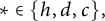 $\ast \in \{h,d,c\},$
 $$ \begin{align} \mathcal{E}_{\ast}(\bar{\alpha};W_{1,1})=(-1)^k \zeta(1+\alpha_3+\alpha_4)\sum_{n=1}^{\infty}\frac{\sigma_{\alpha_1-\alpha_2}(n)}{n^{1+\alpha_1+\alpha_3}} E_{\ast}(n,\alpha_1+\alpha_2,\alpha_3-\alpha_4;W_{1,1}). \end{align} $$
First, we show that
 $\mathcal {E}_{\ast }(\bar {\alpha };W_{1,1})$
converges in a wider range than (7.8). Substituting (5.5) to (7.11) and using (2.8), we prove that
 $$ \begin{align} \mathcal{E}_{h}(\bar{\alpha};W_{1,1})=T_{h}^{1}(\bar{\alpha}), \end{align} $$
where
 $T_{h}^{1}(\bar {\alpha })$
is defined by (7.2). The term
 $T_{h}^{1}(\bar {\alpha })$
converges in the range
 $|\alpha _j|\ll A$
. This follows from the integral representation (5.23), the estimate (4.41), and the fact that
 $W_{1,1}(y)=0$
unless
 $y>x_0$
.
In the next lemma, we investigate the term
 $\mathcal {E}_d(\bar {\alpha };W_{1,1})$
. The term
 $\mathcal {E}_c(\bar {\alpha };W_{1,1})$
converges in the same range of
 $\alpha _j$
since the weight functions in (5.6) and (5.7) coincide.
Lemma 7.2 For
 $$ \begin{align} \Re{\alpha_3}+\Re{\alpha_4}>-1-|\Re{\alpha_1}-\Re{\alpha_2}|, \end{align} $$
one has
 $$ \begin{align} \mathcal{E}_d(\bar{\alpha};W_{1,1})=T_{d}^{1}(\bar{\alpha}), \end{align} $$
where
 $T_{d}^{1}(\bar {\alpha })$
is defined by (7.1).
Proof Substituting (5.6) to (7.11) and using (2.8), we show that the identity (7.14) holds. It remains to prove that (7.1) converges absolutely. To do this, we are going to show that the functions
 $\widehat {W}^{\pm }(t_j)$
decay faster than any fixed power of
 $t_j$
. Due to (5.10), (5.11), and (5.13), it is enough to prove that
 $$ \begin{align} \widehat{W}_{1,1}^{0}(\alpha,\beta;it_j) & = \int_{0}^{\infty}W_{1,1}(y)y^{\frac{\alpha+\beta-1}{2}-it_j} \nonumber\\ &\quad \times {}_2\mathrm{I}_1 \left(\frac{1+\alpha-\beta}{2}+it_j,\frac{1-\alpha-\beta}{2}+it_j,1+2it_j;\frac{-1}{y}\right)dy \nonumber\\ &\quad \ll\frac{1}{t_j^A}, \end{align} $$
where
 $\alpha =\alpha _1+\alpha _2$
and
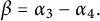 $\beta =\alpha _3-\alpha _4.$
With this goal, we apply (4.44). It is sufficient to consider only the contribution of the main term, since all other terms are of the same form and are smaller in absolute value, while the error term yields the bound
 $t_j^{-A}$
immediately. Therefore, using (2.11) and (6.13), we are left to prove that
 $$ \begin{align} \int_{0}^{\infty} \eta(1/y)\phi_k\left(\frac{1}{1+y};\alpha_1,\alpha_2\right) \frac{y^{-1/4-\alpha_1-\alpha_2+\alpha_3-\alpha_4}(\sqrt{1+y}+\sqrt{y})^{-it_j}}{(1+y)^{5/4-\alpha_1-\alpha_2+3\alpha_3/2-\alpha_4/2}}dy\ll\frac{1}{t_j^A}. \end{align} $$
But this estimate follows directly from multiple integration by parts.
Now, we start to evaluate the main term.
Lemma 7.3 For
 $$ \begin{align} \min(\Re{\alpha_3},\Re{\alpha_4})>\max(\Re{\alpha_1},\Re{\alpha_2}),\quad \min(\Re{\alpha_3},\Re{\alpha_4})>-\min(\Re{\alpha_1},\Re{\alpha_2}), \end{align} $$
one has
 $$ \begin{align} \mathcal{U}(\bar{\alpha};W_{1,1}) &= (-1)^k\mathcal{D}(\alpha_4-\alpha_1)\mathcal{D}(\alpha_4-\alpha_2)\zeta_7(\alpha_1,\alpha_2,\alpha_3,-\alpha_4) \nonumber\\ & \quad\times \int_0^{\infty}W_{1,1}(x)x^{\alpha_1+\alpha_2}(1+x)^{\alpha_3-\alpha_4}dx\nonumber\\ &\quad + (-1)^k\mathcal{D}(\alpha_4+\alpha_1)\mathcal{D}(\alpha_4+\alpha_2)\zeta_7(-\alpha_1,-\alpha_2,\alpha_3,-\alpha_4)\int_0^{\infty}W_{1,1}(x)(1+x)^{\alpha_3-\alpha_4}dx \nonumber\\ &\quad + (-1)^k\mathcal{D}(\alpha_3-\alpha_1)\mathcal{D}(\alpha_3-\alpha_2)\zeta_7(\alpha_1,\alpha_2,-\alpha_3,\alpha_4)\int_0^{\infty}W_{1,1}(x)x^{\alpha_1+\alpha_2}dx \nonumber\\ &\quad + (-1)^k\mathcal{D}(\alpha_3+\alpha_1)\mathcal{D}(\alpha_3+\alpha_2)\zeta_7(-\alpha_1,-\alpha_2,-\alpha_3,\alpha_4)\int_0^{\infty}W_{1,1}(x)dx. \end{align} $$
Proof Substituting (5.3) and (5.4) to (7.10), we obtain four summands. Let us consider the first one (other summands can be treated in the same way):
 $$ \begin{align} & (-1)^k\zeta(1+\alpha_3+\alpha_4)\frac{\zeta(1+\alpha_1+\alpha_2)\zeta(1+\alpha_3-\alpha_4)}{\zeta(2+\alpha_1+\alpha_2+\alpha_3-\alpha_4)} \sum_{n=1}^{\infty}\frac{\sigma_{\alpha_1-\alpha_2}(n)}{n^{1+\alpha_1+\alpha_3}} \sigma_{1+\alpha_1+\alpha_2+\alpha_3-\alpha_4}(n) \nonumber\\ & \qquad\qquad\times \int_0^{\infty}W_{1,1}(x)x^{\alpha_1+\alpha_2}(1+x)^{\alpha_3-\alpha_4}dx. \end{align} $$
Using (2.4), one has
 $$ \begin{align} & \sum_{n=1}^{\infty}\frac{\sigma_{\alpha_1-\alpha_2}(n)}{n^{1+\alpha_1+\alpha_3}} \sigma_{1+\alpha_1+\alpha_2+\alpha_3-\alpha_4}(n) \nonumber\\ &\quad =\frac{\zeta(1+\alpha_1+\alpha_3)}{\zeta(1+\alpha_3+\alpha_4)}\zeta(1+\alpha_3+\alpha_2) \zeta(\alpha_4-\alpha_1)\zeta(\alpha_4-\alpha_2). \end{align} $$
Substituting (7.20) to (7.19), applying (2.3) to
 $\zeta (\alpha _4-\alpha _1)\zeta (\alpha _4-\alpha _2),$
and using the notation (1.3), we obtain the first summand in (7.18).
We are left to evaluate the integrals in (7.18). Unfortunately, it is impossible to express these integrals only in terms of some special functions due to the presence of the function
 $\eta (1/x)$
in
 $W_{1,1}(x)$
. Nevertheless, we can approximate these integrals by the ratio of Gamma factors with a good precision.
Lemma 7.4 The following asymptotic formula holds:
 $$ \begin{align} & \int_0^{\infty}W_{1,1} (x)x^{\alpha_1+\alpha_2}(1+x)^{\alpha_3-\alpha_4}dx \nonumber\\ & \quad = 2(2\pi)^{\alpha_1+\alpha_2-2\alpha_4}X_k(\alpha_4) \Gamma(\alpha_4-\alpha_2)\Gamma(\alpha_4-\alpha_1)\cos\pi\frac{\alpha_1+\alpha_2-2\alpha_4}{2}+O(k^{\epsilon-1}). \end{align} $$
Proof Using (6.9) and (6.13), one has
 $$ \begin{align} & \int_0^{\infty}W_{1,1}(x)x^{\alpha_1+\alpha_2} (1+x)^{\alpha_3-\alpha_4}dx \nonumber\\ &\quad = \int_0^{\infty}\phi_k\left(\frac{1}{1+x};\alpha_1,\alpha_2\right)x^{\alpha_1/2+\alpha_2/2}(1+x)^{-1-\alpha_4}dx \nonumber\\ &\qquad - \int_0^{\infty}\eta(x)\phi_k\left(\frac{1}{1+x};\alpha_1,\alpha_2\right)x^{\alpha_1/2+\alpha_2/2}(1+x)^{-1-\alpha_4}dx. \end{align} $$
To evaluate the first integral, we apply (4.13) and (4.12):
 $$ \begin{align} \int_0^{\infty}\phi_k\left(\frac{1}{1+x};\alpha_1,\alpha_2\right)x^{\alpha_1/2+\alpha_2/2} & (1+x)^{-1-\alpha_4}dx= (2\pi)^{\alpha_1+\alpha_2} \frac{1}{2\pi i}\int_{(\sigma)}\Gamma(k,\alpha_1,\alpha_2;s) \nonumber\\ & \times\sin\left(\pi\frac{s+\alpha_1+\alpha_2}{2}\right) \int_0^{\infty}(1+x)^{-1/2-\alpha_4-s/2}dxds, \end{align} $$
where
 $\max (1-2k,1-2\Re {\alpha _4})<\sigma <1-2\max (|\Re {\alpha _1}|,|\Re {\alpha _2}|)$
. Evaluating the integral over x and substituting (4.11), we infer
 $$ \begin{align} & \int_0^{\infty}\phi_k\left(\frac{1}{1+x};\alpha_1,\alpha_2\right)x^{\alpha_1/2+\alpha_2/2}(1+x)^{-1-\alpha_4}dx \nonumber\\ & \quad = (2\pi)^{\alpha_1+\alpha_2} \frac{1}{2\pi i}\int_{(\sigma)} \frac{\Gamma(k-1/2+s/2)}{\Gamma(k+1/2-s/2)}\nonumber\\ &\quad \Gamma(1/2-\alpha_1-s/2)\Gamma(1/2-\alpha_2-s/2) \frac{\sin\left(\pi\frac{s+\alpha_1+\alpha_2}{2}\right)}{s/2+\alpha_4-1/2}ds. \end{align} $$
Let
 $s=\sigma +iy$
. Using (2.11), one has
 $$ \begin{align} & \frac{\Gamma(k-1/2+s/2)}{\Gamma(k+1/2-s/2)}\Gamma(1/2-\alpha_1-s/2)\Gamma(1/2-\alpha_2-s/2) \frac{\sin\left(\pi\frac{s+\alpha_1+\alpha_2}{2}\right)}{s/2+\alpha_4-1/2} \nonumber\\ &\quad \ll \frac{(k+|y|)^{-1+\sigma}}{(1+|y|)^{1+\Re{\alpha_1}+\Re{\alpha_2}+\sigma}}. \end{align} $$
Moving the line of integration to the left on
 $\Re {s}=2\sigma _1<1-2\Re {\alpha _4}$
, crossing the pole at
 $s=1-2\alpha _4$
, and using the bound (7.25) to estimate the remaining integral, we conclude that
 $$ \begin{align} & \int_0^{\infty}\phi_k\left(\frac{1}{1+x};\alpha_1,\alpha_2\right) x^{\alpha_1/2+\alpha_2/2}(1+x)^{-1-\alpha_4}dx \nonumber\\ &\quad = 2(2\pi)^{\alpha_1+\alpha_2}\frac{\Gamma(k-\alpha_4)}{\Gamma(k+\alpha_4)} \Gamma(\alpha_4-\alpha_2)\Gamma(\alpha_4-\alpha_1)\cos\pi\frac{\alpha_1 +\alpha_2-2\alpha_4}{2} \nonumber\\ &\quad +O(k^{-1-\Re{\alpha_1}-\Re{\alpha_2}}). \end{align} $$
To estimate the second integral in (7.22), we again use (4.13) and (4.12) showing that
 $$ \begin{align} & \int_0^{\infty}\eta(x)\phi_k\left(\frac{1}{1+x};\alpha_1,\alpha_2\right)x^{\alpha_1/2+\alpha_2/2}(1+x)^{-1-\alpha_4}dx \nonumber\\ & \quad =(2\pi)^{\alpha_1+\alpha_2} \frac{1}{2\pi i}\int_{(\sigma)}\Gamma(k,\alpha_1,\alpha_2;s)\sin\left(\pi\frac{s+\alpha_1+\alpha_2}{2}\right) \nonumber\\ &\qquad \times \int_0^{\infty}\eta(x)(1+x)^{-1/2-\alpha_4-s/2}dxds. \end{align} $$
Note that the integral
 $$ \begin{align} \int_0^{\infty}\eta(x)(1+x)^{-1/2-\alpha_4-s/2}dx\ll\frac{1}{1+|\Im{s}|}, \end{align} $$
considered as a function of s, is an entire function. Therefore, moving the line of integration in (7.27) to the left (say on
 $\Re {s}=0$
) and applying (7.25) and (7.28), we obtain
 $$ \begin{align} \int_0^{\infty}\eta(x)\phi_k\left(\frac{1}{1+x};\alpha_1,\alpha_2\right)x^{\alpha_1/2+\alpha_2/2}(1+x)^{-1-\alpha_4}dx\ll k^{-1+\epsilon}. \end{align} $$
Lemma 7.5 The following asymptotic formula holds:
 $$ \begin{align} &\int_0^{\infty}W_{1,1}(x)(1+x)^{\alpha_3-\alpha_4}dx \nonumber\\ &\quad = (2\pi)^{-\alpha_1-\alpha_2-2\alpha_4} X_{k}(\alpha_1)X_{k}(\alpha_2)X_{k}(\alpha_4) \nonumber\\ &\qquad \times \Gamma(\alpha_4+\alpha_2)\Gamma(\alpha_4+\alpha_1)\cos\pi\frac{\alpha_1+\alpha_2+2\alpha_4}{2}+O(k^{\epsilon-1}). \end{align} $$
Proof Using (6.9) and (6.13), one has
 $$ \begin{align} &\int_0^{\infty}W_{1,1}(x)(1+x)^{\alpha_3-\alpha_4}dx \nonumber\\ &\quad = \int_0^{\infty}\phi_k\left(\frac{1}{1+x};\alpha_1,\alpha_2\right)x^{-\alpha_1/2-\alpha_2/2}(1+x)^{-1-\alpha_4}dx \nonumber\\ & \qquad - \int_0^{\infty}\eta(x)\phi_k\left(\frac{1}{1+x};\alpha_1,\alpha_2\right)x^{-\alpha_1/2-\alpha_2/2}(1+x)^{-1-\alpha_4}dx. \end{align} $$
We estimate the second integral first. Applying (4.13) and (4.12), the second integral can be rewritten as
 $$ \begin{align} & \int_0^{\infty}\eta(x)\phi_k\left(\frac{1}{1+x};\alpha_1,\alpha_2\right)x^{-\alpha_1/2-\alpha_2/2}(1+x)^{-1-\alpha_4}dx \nonumber\\ &\quad =(2\pi)^{\alpha_1+\alpha_2} \frac{1}{2\pi i}\int_{(\sigma)}\Gamma(k,\alpha_1,\alpha_2;s)\sin\left(\pi\frac{s+\alpha_1+\alpha_2}{2}\right) \nonumber\\ &\qquad \times\int_0^{\infty}\eta(x)x^{-\alpha_1-\alpha_2}(1+x)^{-1/2-\alpha_4-s/2}dxds. \end{align} $$
To bound the integral over x, we split it into two parts using
 $\eta (x)=\eta _0(x)+\eta _1(x)$
, where
 $\eta _0(x)$
is a smooth function such that
 $$ \begin{align} \eta_0(x)=1\,\text{ for } 0\le x\le \epsilon_0,\quad \eta_0(x)=0\,\text{ for } x> 2\epsilon_0. \end{align} $$
One has
 $$ \begin{align} \int_0^{\infty}\eta_0(x)x^{-\alpha_1-\alpha_2}(1+x)^{-1/2-\alpha_4-s/2}dx\ll\epsilon_0^{1-\Re{\alpha_1}-\Re{\alpha_2}}. \end{align} $$
To estimate the integral with
 $\eta _1(x)$
, we apply the first derivative test (or just integrate by parts once):
 $$ \begin{align} \int_0^{\infty}\eta_1(x)x^{-\alpha_1-\alpha_2}(1+x)^{-1/2-\alpha_4-s/2}dx\ll\frac{\epsilon_0^{-\Re{\alpha_1}-\Re{\alpha_2}}}{1+|\Im{s}+\Im{\alpha_4}|}. \end{align} $$
Choosing
 $\epsilon _0=(1+|\Im {s}+\Im {\alpha _4}|)^{-1}$
, we obtain
 $$ \begin{align} \int_0^{\infty}\eta(x)x^{-\alpha_1-\alpha_2}(1+x)^{-1/2-\alpha_4-s/2}dx\ll(1+|\Im{s}+\Im{\alpha_4}|)^{-1+\Re{\alpha_1}+\Re{\alpha_2}}. \end{align} $$
Substituting (7.36) into (7.32) and estimating the resulting integral using (7.25), we infer
 $$ \begin{align} \int_0^{\infty}\eta(x)\phi_k\left(\frac{1}{1+x};\alpha_1,\alpha_2\right)x^{-\alpha_1/2-\alpha_2/2}(1+x)^{-1-\alpha_4}dx\ll\frac{k^{\epsilon}}{k}. \end{align} $$
To evaluate the first integral on the right-hand side of (7.31), we apply (4.13) and (4.12):
 $$ \begin{align} &\int_0^{\infty}\phi_k \left(\frac{1}{1+x};\alpha_1,\alpha_2\right)x^{-\alpha_1/2-\alpha_2/2}(1+x)^{-1-\alpha_4}dx \nonumber\\ &\quad = (2\pi)^{\alpha_1+\alpha_2} \frac{1}{2\pi i}\int_{(\sigma)}\Gamma(k,\alpha_1,\alpha_2;s) \nonumber\\ & \qquad\times\sin\left(\pi\frac{s+\alpha_1+\alpha_2}{2}\right) \int_0^{\infty}x^{-\alpha_1-\alpha_2}(1+x)^{-1/2-\alpha_4-s/2}dxds, \end{align} $$
where
 $\max (1-2\Re {\alpha _4}-2\Re {\alpha _1}-2\Re {\alpha _2},-1-2\Re {\alpha _4})<\sigma <1-2\max (|\Re {\alpha _1}|,|\Re {\alpha _2}|)$
. To evaluate the integral over x, we use Lemma 2.1, which yields
 $$ \begin{align} &\int_0^{\infty}\phi_k \left(\frac{1}{1+x};\alpha_1,\alpha_2\right)x^{-\alpha_1/2-\alpha_2/2}(1+x)^{-1-\alpha_4}dx \nonumber\\ &\quad = (2\pi)^{\alpha_1+\alpha_2}\Gamma(1-\alpha_1-\alpha_2) \frac{1}{2\pi i}\int_{(\sigma)}\Gamma(k,\alpha_1,\alpha_2;s)\sin\left(\pi\frac{s+\alpha_1+\alpha_2}{2}\right) \nonumber\\ &\qquad \times\frac{\Gamma(-1/2+\alpha_1+\alpha_2+\alpha_4+s/2)}{\Gamma(1/2+\alpha_4+s/2)}ds. \end{align} $$
Moving the line of integration, crossing the pole at
 $s=1-2\alpha _1-2\alpha _2-2\alpha _4$
and estimating the remaining integral using (7.25), we obtain
 $$ \begin{align} &\int_0^{\infty}\phi_k\left(\frac{1}{1+x};\alpha_1,\alpha_2\right)x^{-\alpha_1/2-\alpha_2/2}(1+x)^{-1-\alpha_4}dx \nonumber\\ &\quad = 2(2\pi)^{\alpha_1+\alpha_2}\frac{\Gamma(k-\alpha_1-\alpha_2-\alpha_4)}{\Gamma(k+\alpha_1+\alpha_2+\alpha_4)} \nonumber\\ & \qquad\times \Gamma(\alpha_4+\alpha_2)\Gamma(\alpha_4+\alpha_1)\cos\pi\frac{\alpha_1+\alpha_2+2\alpha_4}{2}+O(k^{\epsilon-1}). \end{align} $$
Applying (1.5) and (2.12), one has
 $$ \begin{align} \frac{\Gamma(k-\alpha_1-\alpha_2-\alpha_4)}{\Gamma(k+\alpha_1+\alpha_2+\alpha_4)}=(2\pi)^{-2\alpha_1-2\alpha_2-2\alpha_4} X_{k}(\alpha_1)X_{k}(\alpha_2)X_{k}(\alpha_4)\left(1+O(k^{-1})\right). \end{align} $$
Now, (7.30) follows from (7.31), (7.37), (7.40), and (7.41).
Lemma 7.6 The following asymptotic formula holds:
 $$ \begin{align} &\int_0^{\infty}W_{1,1}(x)x^{\alpha_1+\alpha_2}dx \nonumber\\ &\quad = 2(2\pi)^{\alpha_1+\alpha_2-2\alpha_3}X_k(\alpha_3) \Gamma(\alpha_3-\alpha_2)\Gamma(\alpha_3-\alpha_1)\cos\pi\frac{\alpha_1+\alpha_2-2\alpha_3}{2} \nonumber\\ &\qquad +O(k^{\epsilon-1}). \end{align} $$
Proof According to (6.9) and (6.13), the integral (7.42) coincides with the right-hand side of (7.22) after changing
 $\alpha _4$
in it by
 $\alpha _3$
. Therefore, the result follows immediately by making this change on the right-hand side of (7.21).
Similarly, after changing
 $\alpha _4$
on the right-hand side of (7.30) by
 $\alpha _3$
, we prove the following result.
Lemma 7.7 One has
 $$ \begin{align} & \int_0^{\infty}W_{1,1}(x)dx \nonumber\\ &\quad =(2\pi)^{-\alpha_1-\alpha_2-2\alpha_3} X_{k}(\alpha_1)X_{k}(\alpha_2)X_{k}(\alpha_3) \Gamma(\alpha_3+\alpha_2)\Gamma(\alpha_3+\alpha_1)\nonumber\\ &\qquad \times \cos\pi\frac{\alpha_1+\alpha_2+2\alpha_3}{2} +O(k^{\epsilon-1}). \end{align} $$
Combining results of Lemmas 7.3–7.7, we finally prove the next lemma.
Lemma 7.8 One has
 $$ \begin{align} \mathcal{U}(\bar{\alpha};W_{1,1})=MU_{1,1}(\bar{\alpha}), \end{align} $$
where
 $MU_{1,1}(\bar {\alpha })$
is defined by (7.5).
The region (7.8) does not contain the most interesting points
 $\Re {\alpha _j}=0$
. The only problem in getting an analytic continuation for (7.9) is the term
 $\mathcal {E}_c(\bar {\alpha };W_{1,1})$
, see (5.20). In order to treat this term, one needs to compute the sum:
 $$ \begin{align} \widehat{W}_{1,1}^{+}(\alpha_1+\alpha_2,\alpha_3-\alpha_4;-i\xi)+\widehat{W}_{1,1}^{-}(\alpha_1+\alpha_2,\alpha_3-\alpha_4;-i\xi) \end{align} $$
at several special points
 $\xi .$
Lemma 7.9 For
 $|\alpha _j|\ll \epsilon $
and
 $\xi _1=\frac {1-\alpha _1+\alpha _2-\alpha _3-\alpha _4}{2}$
, one has
 $$ \begin{align} & \widehat{W}_{1,1}^{+}(\alpha_1+\alpha_2,\alpha_3-\alpha_4;-i\xi_1)+\widehat{W}_{1,1}^{-}(\alpha_1+\alpha_2,\alpha_3-\alpha_4;-i\xi_1) \nonumber\\ &\quad = \frac{\pi}{2}(2\pi)^{\alpha_1+\alpha_2}\Gamma(\alpha_4+\alpha_1)\Gamma(\alpha_4-\alpha_2)\Gamma(\alpha_4+\alpha_3) \frac{\Gamma(k-\alpha_1-\alpha_3-\alpha_4)}{\Gamma(k+\alpha_1+\alpha_3+\alpha_4)} \nonumber\\ &\qquad\times \frac{\cos\pi\frac{\alpha_1-\alpha_2+2\alpha_4}{2}+\cos\pi\frac{\alpha_1+\alpha_2}{2}}{\cos\pi\frac{\alpha_1-\alpha_2+\alpha_3+\alpha_4}{2}} \cos\pi\frac{\alpha_1-\alpha_2+2\alpha_3+2\alpha_4}{2}+O\left(\frac{k^{\epsilon}}{k}\right). \end{align} $$
Proof It follows from (5.12), (5.13), and (6.13) that
 $$ \begin{align} & \widehat{W}_{1,1}^{+}(\alpha_1+\alpha_2,\alpha_3-\alpha_4;-i\xi_1)+\widehat{W}_{1,1}^{-}(\alpha_1+\alpha_2,\alpha_3-\alpha_4;-i\xi_1) \nonumber\\ &\quad =\frac{\pi}{4}\frac{\cos\pi\frac{\alpha_1-\alpha_2+2\alpha_3}{2}-\cos\pi\frac{\alpha_1+\alpha_2}{2}}{\cos\pi\frac{\alpha_1-\alpha_2+\alpha_3+\alpha_4}{2}} \int_{0}^{\infty} \eta(1/y)\phi_k\left(\frac{1}{1+y};\alpha_1,\alpha_2\right) \frac{y^{-1+\alpha_1/2-\alpha_2/2+\alpha_3}}{(1+y)^{1+\alpha_3}} \nonumber\\ & \qquad\times {}_2\mathrm{I}_1 \left(1+\alpha_2-\alpha_3,1-\alpha_1-\alpha_3,2-\alpha_1+\alpha_2-\alpha_3-\alpha_4;\frac{-1}{y}\right)dy \nonumber\\ &\qquad + \frac{\pi}{4}\frac{\cos\pi\frac{\alpha_1-\alpha_2+2\alpha_4}{2}+\cos\pi\frac{\alpha_1+\alpha_2}{2}}{\cos\pi\frac{\alpha_1-\alpha_2+\alpha_3+\alpha_4}{2}} \int_{0}^{\infty} \eta(1/y)\phi_k\left(\frac{1}{1+y};\alpha_1,\alpha_2\right) \frac{y^{-\alpha_1/2+\alpha_2/2-\alpha_4}}{(1+y)^{1+\alpha_3}}\nonumber\\ & \qquad\times {}_2\mathrm{I}_1 \left(\alpha_1+\alpha_4,\alpha_4-\alpha_2,\alpha_1-\alpha_2+\alpha_3+\alpha_4;\frac{-1}{y}\right)dy. \end{align} $$
Let us first consider the second integral in (7.47). Using (2.15), it can be further broken down into the sum of two integrals:

Let us compute the first integral in (7.48). Arguing in the same way as in Lemma 7.5, we show that
 $$ \begin{align} & \frac{\Gamma(\alpha_1+\alpha_4)\Gamma(\alpha_4-\alpha_2)}{\Gamma(\alpha_1-\alpha_2+\alpha_3+\alpha_4)} \int_{0}^{\infty} \eta(1/y)\phi_k\left(\frac{1}{1+y};\alpha_1,\alpha_2\right) \frac{y^{-\alpha_1/2+\alpha_2/2-\alpha_4}}{(1+y)^{1+\alpha_3}}dy \nonumber\\ &\quad = 2(2\pi)^{\alpha_1+\alpha_2}\cos\pi\frac{\alpha_1-\alpha_2+2\alpha_3+2\alpha_4}{2} \Gamma(\alpha_4+\alpha_1)\Gamma(\alpha_4-\alpha_2)\Gamma(\alpha_4+\alpha_3) \nonumber\\ &\qquad \times \frac{\Gamma(k-\alpha_1-\alpha_3-\alpha_4)}{\Gamma(k+\alpha_1+\alpha_3+\alpha_4)}+ O\left(\frac{1}{k^{1+\Re{\alpha_2}-\Re{\alpha_4}}}\right). \end{align} $$
Consider the second integral in (7.48). Making the change of variable
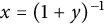 $x=(1+y)^{-1}$
and using the definition (4.17), we obtain the integral
 $$ \begin{align} \int_{0}^{1} Y(x;\alpha_1,\alpha_2)\frac{g(x)}{x^2(1-x)^2}dx, \end{align} $$
where
 $$ \begin{align} g(x)=x^{3/2+\alpha_1/2-\alpha_2/2+\alpha_3+\alpha_4}(1-x)^{1/2-\alpha_1/2+\alpha_2/2-\alpha_4}g_1(1-x), \end{align} $$

Integrating by parts with the help of (4.18), one has to estimate
 $$ \begin{align} \int_{0}^{1} Y(x;\alpha_1,\alpha_2)\frac{d^2}{dx^2}\left( \frac{g(x)}{4x^2(1-x)^2\mathcal{I}(x;\alpha_1,\alpha_2)}\right)dx. \end{align} $$
It follows from (4.19) that
 $$ \begin{align} 4x^2(1-x)^2\mathcal{I}(x;\alpha_1,\alpha_2)=(2k-1)^2x(1-x)+p_2(x), \end{align} $$
where
 $p_2(x)=x^2-(1+4\alpha _1\alpha _2)x+1-(\alpha _2-\alpha _1)^2$
. Evaluating the second derivative in (7.53), we show that
 $$ \begin{align} \frac{d^2}{dx^2}\left( \frac{g(x)}{4x^2(1-x)^2\mathcal{I}(x;\alpha_1,\alpha_2)}\right)\ll\frac{x^{-1/2+\Re{(\alpha_1/2-\alpha_2/2+\alpha_3+\alpha_4)}}}{(2k-1)^2x(1-x)+p_2(x)}. \end{align} $$
Using (7.55), (4.17), and Lemma 4.5, we prove that the integral (7.53) is bounded by
 $$ \begin{align} \int_{0}^{1}\eta\left(\frac{x}{1-x}\right)\phi_k\left(x;\alpha_1,\alpha_2\right) \frac{x^{-1/2+\Re{(\alpha_1/2-\alpha_2/2+\alpha_3+\alpha_4)}}}{k^2x+1}dx\ll\frac{1}{k^{2+2\Re{(\alpha_1+\alpha_3+\alpha_4)}}}. \end{align} $$
We are left to estimate the first integral in (7.47). Comparing it with the second integral in (7.48), we see that they are quite similar, and thus an estimate like (7.56) can also be obtained for the first integral in (7.47).
Lemma 7.10 For
 $|\alpha _j|\ll \epsilon $
and
 $\xi _2=\frac {1+\alpha _1-\alpha _2-\alpha _3-\alpha _4}{2}$
, one has
 $$ \begin{align} & \widehat{W}_{1,1}^{+}(\alpha_1+\alpha_2,\alpha_3-\alpha_4;-i\xi_2)+\widehat{W}_{1,1}^{-}(\alpha_1+\alpha_2,\alpha_3-\alpha_4;-i\xi_2) \nonumber\\ &\quad = \frac{\pi}{2}(2\pi)^{\alpha_1+\alpha_2}\Gamma(\alpha_4+\alpha_2)\Gamma(\alpha_4-\alpha_1)\Gamma(\alpha_4+\alpha_3) \frac{\Gamma(k-\alpha_2-\alpha_3-\alpha_4)}{\Gamma(k+\alpha_2+\alpha_3+\alpha_4)} \nonumber\\ &\qquad \times \frac{\cos\pi\frac{\alpha_2-\alpha_1+2\alpha_4}{2}+\cos\pi\frac{\alpha_1+\alpha_2}{2}}{\cos\pi\frac{\alpha_2-\alpha_1+\alpha_3+\alpha_4}{2}} \cos\pi\frac{\alpha_2-\alpha_1+2\alpha_3+2\alpha_4}{2}+O\left(\frac{k^{\epsilon}}{k}\right). \end{align} $$
Proof Using (6.13) and (3.6), we show that
 $$ \begin{align} W_{1,1}(\alpha_1,\alpha_2,\alpha_3,\alpha_4;x)=W_{1,1}(\alpha_2,\alpha_1,\alpha_3,\alpha_4;x). \end{align} $$
Therefore, (7.57) follows from (7.46) by making the change of variable
 $\alpha _1\leftrightarrow \alpha _2$
.
Now, we are ready to provide an analytic continuation for
 $\mathcal {E}_c(\bar {\alpha };W_{1,1})$
, which is given in the following lemma.
Lemma 7.11 For
 $|\alpha _j|\ll \epsilon $
, one has
 $$ \begin{align} \mathcal{E}_{c}(\bar{\alpha};W_{1,1})=\mathbf{S}_{1,1}(\bar{\alpha})+T_{c}^{1}(\bar{\alpha}), \end{align} $$
where
 $\mathbf {S}_{1,1}(\bar {\alpha })$
and
 $T_{c}^{1}(\bar {\alpha })$
are defined by (7.6) and (7.3), respectively.
Proof Substituting (5.7) to (7.11), evaluating the resulting sum over n with the use of (2.4), we show that for
 $$ \begin{align} \Re{\alpha_3}+\Re{\alpha_4}>1+|\Re{\alpha_1}-\Re{\alpha_2}|,\quad \Re{\alpha_3}-\Re{\alpha_4}>-1+|\Re{\alpha_1}+\Re{\alpha_2}|, \end{align} $$
the following identity holds:
 $$ \begin{align} \mathcal{E}_{c}(\bar{\alpha};W_{1,1})&=\frac{4(-1)^k(2\pi)^{\alpha_3-\alpha_4-1}}{2\pi i}\int_{(0)} \mathcal{F}_{1,1}(\bar{\alpha};\xi) \nonumber\\ &\quad \times \left(\widehat{W}_{1,1}^{+}(\alpha_1+\alpha_2,\alpha_3-\alpha_4;-i\xi)+\widehat{W}_{1,1}^{-}(\alpha_1+\alpha_2,\alpha_3-\alpha_4;-i\xi)\right)d\xi. \end{align} $$
The function
 $\mathcal {F}_{1,1}(\bar {\alpha };\xi )$
has eight poles. In both cases, when the parameters
 $\alpha _j$
belong to the region (7.60) or to the region
 $$ \begin{align} \Re{\alpha_3}+\Re{\alpha_4}<1-|\Re{\alpha_1}-\Re{\alpha_2}|,\quad \Re{\alpha_3}-\Re{\alpha_4}>-1+|\Re{\alpha_1}+\Re{\alpha_2}|, \end{align} $$
two of the poles of
 $\mathcal {Z}_4(\alpha _1+\alpha _2,\alpha _3-\alpha _4,\xi )$
are located in the half-plane
 $\Re {\xi }>0$
and two other poles are located in the half-plane
 $\Re {\xi }<0$
. While the remaining four poles
 $$ \begin{align} \xi_1=\frac{1-\alpha_1+\alpha_2-\alpha_3-\alpha_4}{2},\, \xi_2=\frac{1+\alpha_1-\alpha_2-\alpha_3-\alpha_4}{2},\, \xi_3=-\xi_1,\,\xi_4=-\xi_2 \end{align} $$
change their location from one half-plane to another when the parameters
 $\alpha _j$
pass from the region (7.60) to the region (7.62). To obtain an analytic continuation for
 $\mathcal {E}_{c}(\bar {\alpha };W_{1,1})$
to the region (7.62), we use a variant of the Sokhotski–Plemelj theorem [Reference Cima, Matheson and Ross7, Corollary 2.4.2, p. 55]. Arguing in the same way as in [Reference Balkanova and Frolenkov3, Theorem 6.2], we show that, in the region (7.62), the following formula holds:
 $$ \begin{align} \mathcal{E}_{c}(\bar{\alpha};W_{1,1}) & = 4(-1)^k(2\pi)^{\alpha_3-\alpha_4-1}\left(R_{1,1}(\xi_1)-R_{1,1}(\xi_3)+R_{1,1}(\xi_2)-R_{1,1}(\xi_4)\right) \nonumber\\ &\qquad +4(-1)^k \frac{(2\pi)^{\alpha_3-\alpha_4-1}}{2\pi i}\int_{(0)} \mathcal{F}_{1,1}(\bar{\alpha};\xi) \nonumber\\ &\qquad \times\left(\widehat{W}_{1,1}^{+}(\alpha_1+\alpha_2,\alpha_3-\alpha_4;-i\xi)+\widehat{W}_{1,1}^{-}(\alpha_1+\alpha_2,\alpha_3-\alpha_4;-i\xi)\right)d\xi, \end{align} $$
where
 $$ \begin{align} R_{1,1}(\xi_k) &= \operatorname{\mathrm{res}}_{\xi_k}\mathcal{F}_{1,1}(\bar{\alpha};\xi) \nonumber\\ &\quad \times\left(\widehat{W}_{1,1}^{+}(\alpha_1+\alpha_2,\alpha_3-\alpha_4;-i\xi) + \widehat{W}_{1,1}^{-}(\alpha_1+\alpha_2,\alpha_3-\alpha_4;-i\xi)\right). \end{align} $$
Using (2.3) and (1.3), one has
 $$ \begin{align} R_{1,1}(\xi_1) &= \zeta_7(-\alpha_1,\alpha_2,-\alpha_3,-\alpha_4)\mathcal{D}(\alpha_4+\alpha_1)\mathcal{D}(\alpha_4-\alpha_2)\mathcal{D}(\alpha_4+\alpha_3) \nonumber\\ &\quad \times \left(\widehat{W}_{1,1}^{+}(\alpha_1+\alpha_2,\alpha_3-\alpha_4;-i\xi_1)+\widehat{W}_{1,1}^{-}(\alpha_1+\alpha_2,\alpha_3-\alpha_4;-i\xi_1)\right), \end{align} $$
 $$ \begin{align} R_{1,1}(\xi_2) &= \zeta_7(\alpha_1,-\alpha_2,-\alpha_3,-\alpha_4)\mathcal{D}(\alpha_4-\alpha_1)\mathcal{D}(\alpha_4+\alpha_2)\mathcal{D}(\alpha_4+\alpha_3) \nonumber\\ & \quad \times \left(\widehat{W}_{1,1}^{+}(\alpha_1+\alpha_2,\alpha_3-\alpha_4;-i\xi_2)+\widehat{W}_{1,1}^{-}(\alpha_1+\alpha_2,\alpha_3-\alpha_4;-i\xi_2)\right), \end{align} $$
 $$ \begin{align} R_{1,1}(\xi_3)=-R_{1,1}(\xi_1),\quad R_{1,1}(\xi_4)=-R_{1,1}(\xi_2). \end{align} $$
In order to simplify the evaluation of
 $R_{1,1}(\xi _1)$
and
 $R_{1,1}(\xi _2)$
, we restrict the parameters
 $\alpha _j$
to the range
 $|\alpha _j|\ll \epsilon $
instead of the wider range (7.62). Using (7.46), (2.3), (7.41) and the relation
 $$ \begin{align} \cos\pi\frac{\alpha_1-\alpha_2+2\alpha_4}{2}+\cos\pi\frac{\alpha_1+\alpha_2}{2}=2\cos\pi\frac{\alpha_1+\alpha_4}{2}\cos\pi\frac{\alpha_4-\alpha_2}{2}, \end{align} $$
we infer
 $$ \begin{align} & 4(-1)^k(2\pi)^{\alpha_3-\alpha_4-1} \left(R_{1,1}(\xi_1)-R_{1,1}(\xi_3)\right) \nonumber\\ &\quad = \frac{\cos\pi\frac{\alpha_1-\alpha_2+2\alpha_3+2\alpha_4}{2}}{2\cos\pi\frac{\alpha_4+\alpha_3}{2}\cos\pi\frac{\alpha_1-\alpha_2+\alpha_3+\alpha_4}{2}} \nonumber\\ &\qquad\times \mathcal{C}(-\alpha_1,\alpha_2,-\alpha_3,-\alpha_4)\zeta_7(-\alpha_1,\alpha_2,-\alpha_3,-\alpha_4)+O\left(\frac{k^{\epsilon}}{k}\right). \end{align} $$
Using (7.57), (2.3), (7.41) (with
 $\alpha _1$
replaced by
 $\alpha _2$
) and the relation
 $$ \begin{align} \cos\pi\frac{\alpha_2-\alpha_1+2\alpha_4}{2}+\cos\pi\frac{\alpha_1+\alpha_2}{2}=2\cos\pi\frac{\alpha_2+\alpha_4}{2}\cos\pi\frac{\alpha_4-\alpha_1}{2}, \end{align} $$
we prove
 $$ \begin{align} & 4(-1)^k(2\pi)^{\alpha_3-\alpha_4-1} \left(R_{1,1}(\xi_2)-R_{1,1}(\xi_4)\right) \nonumber\\ &\quad = \frac{\cos\pi\frac{\alpha_2-\alpha_1+2\alpha_3+2\alpha_4}{2}}{2\cos\pi\frac{\alpha_4+\alpha_3}{2}\cos\pi\frac{\alpha_2-\alpha_1+\alpha_3+\alpha_4}{2}} \nonumber\\ &\qquad \times \mathcal{C}(\alpha_1,-\alpha_2,-\alpha_3,-\alpha_4)\zeta_7(\alpha_1,-\alpha_2,-\alpha_3,-\alpha_4) +O\left(\frac{k^{\epsilon}}{k}\right). \end{align} $$
8 Analysis of
$\mathcal {TD}^{(1,2)}$

It follows from (4.1), (6.13), and (6.15) that
 $$ \begin{align} W_{1,2}(\alpha_1,\alpha_2,\alpha_3,\alpha_4;x)=(-1)^kX_k(\alpha_2)W_{1,1}(\alpha_1,-\alpha_2,\alpha_3,\alpha_4;x). \end{align} $$
Then, one has (see (6.12) and (6.14))
 $$ \begin{align} \mathcal{TD}^{(1,2)}(\alpha_1,\alpha_2,\alpha_3,\alpha_4)=(-1)^kX_k(\alpha_2)\mathcal{TD}^{(1,1)}(\alpha_1,-\alpha_2,\alpha_3,\alpha_4). \end{align} $$
We are left to understand how the coefficients
 $\mathcal {C}(\epsilon _1\alpha _1,\epsilon _2\alpha _2,\epsilon _3\alpha _3,\epsilon _4\alpha _4)$
, defined by (1.4), change if one changes the sign
 $\epsilon _2$
and multiplies by
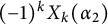 $(-1)^kX_k(\alpha _2)$
. The coefficient
 $\mathcal {C}(\ast ,\alpha _2,\ast ,\ast )$
does not contain
 $X_k(\alpha _2)$
, so it does not change after the sign change of
 $\alpha _2$
, and being multiplied by
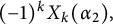 $(-1)^kX_k(\alpha _2),$
it becomes
 $\mathcal {C}(\ast ,-\alpha _2,\ast ,\ast )$
. The coefficient
 $\mathcal {C}(\ast ,-\alpha _2,\ast ,\ast )$
contains
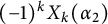 $(-1)^kX_k(\alpha _2)$
, so after the sign change of
 $\alpha _2$
and multiplication by
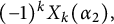 $(-1)^kX_k(\alpha _2),$
we obtain
 $\mathcal {C}(\ast ,\alpha _2,\ast ,\ast )$
since
 $$ \begin{align*}(-1)^kX_k(-\alpha_2)(-1)^kX_k(\alpha_2)=1.\end{align*} $$
This means that we just need to change
 $\alpha _2$
by
 $-\alpha _2$
in (7.5) and (7.6). Keeping this in mind and using (7.9)), we finally derive the following decomposition.
Lemma 8.1 For
 $|\alpha _j|\ll \epsilon ,$
one has
 $$ \begin{align} &\mathcal{TD}^{(1,2)}(\alpha_1,\alpha_2,\alpha_3,\alpha_4) \nonumber\\ &\quad = MU_{1,2}(\bar{\alpha})+\mathbf{S}_{1,2}(\bar{\alpha})+ (-1)^kX_k(\alpha_2) \left(T_{h}^{1}+T_{d}^{1}+T_{c}^{1}\right)&(\alpha_1,-\alpha_2,\alpha_3,\alpha_4) \nonumber\\ & \quad + O(k^{\epsilon-1}), \end{align} $$
where
 $T_{h}^{1}(\bar {\alpha })$
,
 $T_{d}^{1}(\bar {\alpha }),$
and
 $T_{c}^{1}(\bar {\alpha })$
are given by (7.2), (7.1), and (7.3), respectively, and
 $$ \begin{align} MU_{1,2}(\bar{\alpha}) &:= \mathcal{C}(\alpha_1,-\alpha_2,\alpha_3,-\alpha_4)\zeta_7(\alpha_1,-\alpha_2,\alpha_3,-\alpha_4) \frac{\cos\pi\frac{\alpha_2-\alpha_1+2\alpha_4}{2}}{2\cos\pi\frac{\alpha_4-\alpha_1}{2}\cos\pi\frac{\alpha_4+\alpha_2}{2}} \nonumber\\ & \quad + \mathcal{C}(-\alpha_1,\alpha_2,\alpha_3,-\alpha_4)\zeta_7(-\alpha_1,\alpha_2,\alpha_3,-\alpha_4) \frac{\cos\pi\frac{\alpha_1-\alpha_2+2\alpha_4}{2}}{2\cos\pi\frac{\alpha_4+\alpha_1}{2}\cos\pi\frac{\alpha_4-\alpha_2}{2}} \nonumber\\ & \quad + \mathcal{C}(\alpha_1,-\alpha_2,-\alpha_3,\alpha_4)\zeta_7(\alpha_1,-\alpha_2,-\alpha_3,\alpha_4) \frac{\cos\pi\frac{\alpha_2-\alpha_1+2\alpha_3}{2}}{2\cos\pi\frac{\alpha_3-\alpha_1}{2}\cos\pi\frac{\alpha_3+\alpha_2}{2}} \nonumber\\ & \quad + \mathcal{C}(-\alpha_1,\alpha_2,-\alpha_3,\alpha_4)\zeta_7(-\alpha_1,\alpha_2,-\alpha_3,\alpha_4) \frac{\cos\pi\frac{\alpha_1-\alpha_2+2\alpha_3}{2}}{2\cos\pi\frac{\alpha_3+\alpha_1}{2}\cos\pi\frac{\alpha_3-\alpha_2}{2}}, \end{align} $$
 $$ \begin{align} \mathbf{S}_{1,2}(\bar{\alpha}) & := \mathcal{C}(-\alpha_1,-\alpha_2,-\alpha_3,-\alpha_4)\zeta_7(-\alpha_1,-\alpha_2,-\alpha_3,-\alpha_4) \nonumber\\ &\quad \times\frac{\cos\pi\frac{\alpha_1+\alpha_2+2\alpha_3+2\alpha_4}{2}}{2\cos\pi\frac{\alpha_4+\alpha_3}{2}\cos\pi\frac{\alpha_1+\alpha_2+\alpha_3+\alpha_4}{2}} \nonumber\\ & \quad + \mathcal{C}(\alpha_1,\alpha_2,-\alpha_3,-\alpha_4)\zeta_7(\alpha_1,\alpha_2,-\alpha_3,-\alpha_4) \frac{\cos\pi\frac{-\alpha_2-\alpha_1+2\alpha_3+2\alpha_4}{2}}{2\cos\pi\frac{\alpha_4+\alpha_3}{2}\cos\pi\frac{-\alpha_2-\alpha_1+\alpha_3+\alpha_4}{2}}. \end{align} $$
9 Analysis of
$\mathcal {TD}^{(2,1)}$

In order to describe discrete and holomorphic contributions coming from the term (6.16), we introduce the following weighted fourth moments of L-functions associated with Maass and holomorphic cusp forms:
 $$ \begin{align} T_{d}^{2}(\bar{\alpha}) & := 2(2\pi)^{\alpha_1-\alpha_2-1} \sum_{j} \omega_j L_j\left(\frac{1-\alpha_1+\alpha_2+\alpha_3-\alpha_4}{2}\right) \nonumber\\ &\quad \times L_j\left(\frac{1-\alpha_1+\alpha_2-\alpha_3+\alpha_4}{2}\right) L_j\left(\frac{1-\alpha_1-\alpha_2+\alpha_3+\alpha_4}{2}\right)\nonumber\\ &\quad \times L_j\left(\frac{1+\alpha_1+\alpha_2+\alpha_3+\alpha_4}{2}\right) \nonumber\\ &\quad \times \left(\widehat{W}_{2,1}^{+}+\varepsilon_j\widehat{W}_{2,1}^{-}\right)(\alpha_3-\alpha_4,\alpha_1-\alpha_2;t_j), \end{align} $$
 $$ \begin{align} T_{h}^{2}(\bar{\alpha}) & :=2(2\pi)^{\alpha_1-\alpha_2-1} \sum_{m=6}^{\infty}\frac{2m-1}{\pi^2}\sum_{f\in H_{2m}} \omega_f L_f\left(\frac{1-\alpha_1+\alpha_2+\alpha_3-\alpha_4}{2}\right) \nonumber\\ &\quad \times L_f\left(\frac{1-\alpha_1+\alpha_2-\alpha_3+\alpha_4}{2}\right) L_f\left(\frac{1-\alpha_1-\alpha_2+\alpha_3+\alpha_4}{2}\right) \nonumber\\ &\quad \times L_f\left(\frac{1+\alpha_1+\alpha_2+\alpha_3+\alpha_4}{2}\right) \nonumber\\ & \quad \times \widehat{W}_{2,1}(\alpha_3-\alpha_4,\alpha_1-\alpha_2;m). \end{align} $$
The continuous contribution is given by the weighted eighth moment of the Riemann zeta function:
 $$ \begin{align} T_{c}^{2}(\bar{\alpha}) & := \frac{4(-1)^k(2\pi)^{\alpha_1-\alpha_2-1}}{2\pi i}\int_{(0)} \mathcal{F}_{2,1}(\bar{\alpha};\xi) \nonumber\\ &\quad \times \left(\widehat{W}_{2,1}^{+}(\alpha_3-\alpha_4,\alpha_1-\alpha_2;-i\xi)+\widehat{W}_{2,1}^{-}(\alpha_3-\alpha_4,\alpha_1-\alpha_2;-i\xi)\right)d\xi, \end{align} $$
where
 $$ \begin{align} \mathcal{F}_{2,1}(\bar{\alpha};\xi) &= \zeta\left(\frac{1+\alpha_1+\alpha_2+\alpha_3+\alpha_4}{2}+\xi\right) \zeta\left(\frac{1-\alpha_1-\alpha_2+\alpha_3+\alpha_4}{2}+\xi\right) \nonumber\\ & \quad\times \zeta\left(\frac{1+\alpha_1+\alpha_2+\alpha_3+\alpha_4}{2}-\xi\right) \zeta\left(\frac{1-\alpha_1-\alpha_2+\alpha_3+\alpha_4}{2}-\xi\right) \nonumber\\ &\quad \times\frac{\mathcal{Z}_4(\alpha_3-\alpha_4,\alpha_1-\alpha_2,\xi)}{\zeta(1+2\xi)\zeta(1-2\xi)}, \end{align} $$
and
 $\mathcal {Z}_4(\alpha ,\beta ,\xi )$
is the product of four Riemann zeta functions defined by (5.8).
Recall that the function
 $W_{2,1}(y)$
is defined by (6.17) and its transforms used in the definitions of (9.1)–(9.3) are given in Theorem 5.1.
Finally, in order to state the main result of this section, we introduce the following terms:
 $$ \begin{align} MU_{2,1}(\bar{\alpha}) &:= \mathcal{C}(\alpha_1,-\alpha_2,\alpha_3,-\alpha_4)\zeta_7(\alpha_1,-\alpha_2,\alpha_3,-\alpha_4) \frac{\cos\pi\frac{\alpha_1+\alpha_2}{2}}{2\cos\pi\frac{\alpha_4+\alpha_2}{2}\cos\pi\frac{\alpha_4-\alpha_1}{2}} \nonumber\\ &\quad + \mathcal{C}(\alpha_1,-\alpha_2,-\alpha_3,\alpha_4)\zeta_7(\alpha_1,-\alpha_2,-\alpha_3,\alpha_4) \frac{\cos\pi\frac{\alpha_1+\alpha_2}{2}}{2\cos\pi\frac{\alpha_3-\alpha_1}{2}\cos\pi\frac{\alpha_3+\alpha_2}{2}} \nonumber\\ &\quad + \mathcal{C}(-\alpha_1,\alpha_2,\alpha_3,-\alpha_4)\zeta_7(-\alpha_1,\alpha_2,\alpha_3,-\alpha_4) \frac{\cos\pi\frac{\alpha_1+\alpha_2}{2}}{2\cos\pi\frac{\alpha_4+\alpha_1}{2}\cos\pi\frac{\alpha_4-\alpha_2}{2}} \nonumber\\ &\quad +\mathcal{C}(-\alpha_1,\alpha_2,-\alpha_3,\alpha_4)\zeta_7(-\alpha_1,\alpha_2,-\alpha_3,\alpha_4) \frac{\cos\pi\frac{\alpha_1+\alpha_2}{2}}{2\cos\pi\frac{\alpha_3+\alpha_1}{2}\cos\pi\frac{\alpha_3-\alpha_2}{2}} \end{align} $$
and
 $$ \begin{align} \mathbf{S}_{2,1}(\bar{\alpha}) &= \mathcal{C}(-\alpha_1,-\alpha_2,-\alpha_3,-\alpha_4)\zeta_7(-\alpha_1,-\alpha_2,-\alpha_3,-\alpha_4) \nonumber\\ &\quad \times\frac{\cos\pi\frac{\alpha_1+\alpha_2}{2}}{2\cos\pi\frac{\alpha_4+\alpha_3}{2}\cos\pi\frac{\alpha_1+\alpha_2+\alpha_3+\alpha_4}{2}} \nonumber\\ & \quad + \mathcal{C}(\alpha_1,\alpha_2,-\alpha_3,-\alpha_4)\zeta_7(\alpha_1,\alpha_2,-\alpha_3,-\alpha_4) \frac{\cos\pi\frac{\alpha_1+\alpha_2}{2}}{2\cos\pi\frac{\alpha_4+\alpha_3}{2}\cos\pi\frac{\alpha_1+\alpha_2-\alpha_3-\alpha_4}{2}}, \end{align} $$
where
 $\zeta _7(\epsilon _1\alpha _1,\epsilon _2\alpha _2,\epsilon _3\alpha _3,\epsilon _4\alpha _4)$
and
 $\mathcal {C}(\epsilon _1\alpha _1,\epsilon _2\alpha _2,\epsilon _3\alpha _3,\epsilon _4\alpha _4)$
are defined by (1.3) and (1.4), respectively.
Lemma 9.1 For
 $|\alpha _j|\ll \epsilon ,$
one has
 $$ \begin{align} \mathcal{TD}^{(2,1)}(\bar{\alpha})=MU_{2,1}(\bar{\alpha})+\mathbf{S}_{2,1}(\bar{\alpha})+T_{d}^{2}(\bar{\alpha})+T_{h}^{2}(\bar{\alpha})+T_{c}^{2}(\bar{\alpha}). \end{align} $$
In order to prove Lemma 9.1, we apply Theorem 5.1. Accordingly, for
 $$ \begin{align} \min_{j=3,4}\Re{\alpha_j}>1+\frac{1}{2}|\Re{\alpha_1}+\Re{\alpha_2}|+\frac{1}{2}|\Re{\alpha_1}-\Re{\alpha_2}|,\quad |\Re{\alpha_3}-\Re{\alpha_4}|<1+\Re{\alpha_1}-\Re{\alpha_2,} \end{align} $$
one has
 $$ \begin{align} \mathcal{TD}^{(2,1)}(\bar{\alpha})=\mathcal{U}(\bar{\alpha};W_{2,1})+\mathcal{E}_h(\bar{\alpha};W_{2,1})+\mathcal{E}_d(\bar{\alpha};W_{2,1})+\mathcal{E}_c(\bar{\alpha};W_{2,1}), \end{align} $$
where
 $$ \begin{align} \mathcal{U}(\bar{\alpha};W_{2,1})= \zeta(1+\alpha_3+\alpha_4)\sum_{n=1}^{\infty} \frac{\sigma_{\alpha_1+\alpha_2}(n)}{n^{1+\alpha_1+\alpha_3}}U(n,\alpha_3-\alpha_4,\alpha_1-\alpha_2;W_{2,1}), \end{align} $$
and for
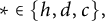 $\ast \in \{h,d,c\},$
 $$ \begin{align} \mathcal{E}_{\ast}(\bar{\alpha};W_{2,1})=(-1)^k \zeta(1+\alpha_3+\alpha_4)\sum_{n=1}^{\infty}\frac{\sigma_{\alpha_1+\alpha_2}(n)}{n^{1+\alpha_1+\alpha_3}} E_{\ast}(n,\alpha_3-\alpha_4,\alpha_1-\alpha_2;W_{2,1}). \end{align} $$
Substituting (5.5) to (9.11) and using (2.8), we show that
 $$ \begin{align} \mathcal{E}_{h}(\bar{\alpha};W_{2,1})=T_{h}^2(\bar{\alpha}), \end{align} $$
where
 $T_{h}^2(\bar {\alpha })$
is defined by (9.2).
The term
 $T_{h}^2(\bar {\alpha })$
converges in the range
 $|\alpha _j|\ll A$
. This follows from the integral representation (5.23) and the estimate (4.41) since
 $W_{2,1}(y)=0$
unless
 $y>x_0$
. In the next lemma, we investigate the term
 $\mathcal {E}_d(\bar {\alpha };W_{2,1})$
. The term
 $\mathcal {E}_c(\bar {\alpha };W_{2,1})$
converges in the same range of
 $\alpha _j$
because the weight functions in (5.6) and (5.7) coincide.
The following result can be proved in the same way as Lemma 7.2.
Lemma 9.2 For
 $$ \begin{align} \Re{\alpha_3}+\Re{\alpha_4}>-1+|\Re{\alpha_1}+\Re{\alpha_2}|, \end{align} $$
one has
 $$ \begin{align} \mathcal{E}_d(\bar{\alpha};W_{2,1})=T_{d}^{2}(\bar{\alpha}), \end{align} $$
where
 $T_{d}^{2}(\bar {\alpha })$
is defined by (9.1).
Lemma 9.3 For
 $$ \begin{align} 2\min(\Re{\alpha_3},\Re{\alpha_4})>|\Re{\alpha_1}+\Re{\alpha_2}|+|\Re{\alpha_1}-\Re{\alpha_2}|, \end{align} $$
the following identity holds:
 $$ \begin{align} & \mathcal{U}(\bar{\alpha};W_{2,1}) \nonumber\\ &\quad =\mathcal{D}(\alpha_4-\alpha_1)\mathcal{D}(\alpha_4+\alpha_2)\zeta_7(\alpha_1,-\alpha_2,\alpha_3,-\alpha_4) \int_0^{\infty}W_{2,1}(x)x^{\alpha_3-\alpha_4}(1+x)^{\alpha_1-\alpha_2}dx \nonumber\\ & \quad + \mathcal{D}(\alpha_3-\alpha_1)\mathcal{D}(\alpha_3+\alpha_2)\zeta_7(\alpha_1,-\alpha_2,-\alpha_3,\alpha_4)\int_0^{\infty}W_{2,1}(x)(1+x)^{\alpha_1-\alpha_2}dx \nonumber\\ &\quad + \mathcal{D}(\alpha_4+\alpha_1)\mathcal{D}(\alpha_4-\alpha_2)\zeta_7(-\alpha_1,\alpha_2,\alpha_3,-\alpha_4)\int_0^{\infty}W_{2,1}(x)x^{\alpha_3-\alpha_4}dx \nonumber\\ &\quad + \mathcal{D}(\alpha_3+\alpha_1)\mathcal{D}(\alpha_3-\alpha_2)\zeta_7(-\alpha_1,\alpha_2,-\alpha_3,\alpha_4)\int_0^{\infty}W_{2,1}(x)dx.\nonumber\\ \end{align} $$
Proof Substituting (5.3) and (5.4) to (9.10), we obtain four summands. Let us consider the first one (other summands can be treated in the same way):
 $$ \begin{align} &\zeta(1+\alpha_3+\alpha_4)\frac{\zeta(1+\alpha_1-\alpha_2)\zeta(1+\alpha_3-\alpha_4)}{\zeta(2+\alpha_1-\alpha_2+\alpha_3-\alpha_4)} \sum_{n=1}^{\infty}\frac{\sigma_{\alpha_1+\alpha_2}(n)}{n^{1+\alpha_1+\alpha_3}} \sigma_{1+\alpha_1-\alpha_2+\alpha_3-\alpha_4}(n) \nonumber\\ & \quad \times \int_0^{\infty}W_{2,1}(x)x^{\alpha_3-\alpha_4}(1+x)^{\alpha_1-\alpha_2}dx. \end{align} $$
Using (2.4), one has
 $$ \begin{align} & \sum_{n=1}^{\infty}\frac{\sigma_{\alpha_1+\alpha_2}(n)}{n^{1+\alpha_1+\alpha_3}} \sigma_{1+\alpha_1-\alpha_2+\alpha_3-\alpha_4}(n) \nonumber\\ &\quad =\frac{\zeta(1+\alpha_1+\alpha_3)}{\zeta(1+\alpha_3+\alpha_4)}\zeta(1+\alpha_3-\alpha_2) \zeta(\alpha_4-\alpha_1)\zeta(\alpha_4+\alpha_2). \end{align} $$
Substituting (9.18) to (9.17), applying (2.3) to the product
 $\zeta (\alpha _4-\alpha _1)\zeta (\alpha _4+\alpha _2),$
and using the notation (1.3), we obtain the first summand in (9.16).
Lemma 9.4 The following asymptotic formula holds:
 $$ \begin{align} &\int_0^{\infty}W_{2,1}(x)x^{\alpha_3-\alpha_4}(1+x)^{\alpha_1-\alpha_2}dx \nonumber\\ &\quad = 2(2\pi)^{\alpha_1-\alpha_2-2\alpha_4}X_k(\alpha_2)X_k(\alpha_4) \Gamma(\alpha_4-\alpha_1)\Gamma(\alpha_4+\alpha_2)\cos\pi\frac{\alpha_1+\alpha_2}{2} \nonumber\\ &\quad +O(k^{-2}). \end{align} $$
Proof Using (6.9) and (6.17), we have
 $$ \begin{align} &\int_0^{\infty}W_{2,1}(x)x^{\alpha_3-\alpha_4} (1+x)^{\alpha_1-\alpha_2}dx \nonumber\\ &\quad = \int_0^{\infty}\Phi_k\left(\frac{x}{1+x};\alpha_1,\alpha_2\right)(1+x)^{\alpha_1/2-\alpha_2/2}x^{-1-\alpha_4}dx \nonumber\\ &\quad - \int_0^{\infty}\eta(x)\Phi_k\left(\frac{x}{1+x};\alpha_1,\alpha_2\right)(1+x)^{\alpha_1/2-\alpha_2/2}x^{-1-\alpha_4}dx. \end{align} $$
To evaluate the first integral, we use (4.14) and (4.12). As a result, one has
 $$ \begin{align} &\int_0^{\infty}\Phi_k\left(\frac{x}{1+x};\alpha_1,\alpha_2\right) (1+x)^{\alpha_1/2-\alpha_2/2}x^{-1-\alpha_4}dx \nonumber\\ &\quad = (-1)^k(2\pi)^{\alpha_1+\alpha_2} \frac{1}{2\pi i}\int_{(\sigma)}\Gamma(k,\alpha_1,\alpha_2;s) \nonumber\\ & \quad \times\sin\left(\pi\frac{s+\alpha_1+\alpha_2}{2}\right) \int_0^{\infty}x^{-1/2-\alpha_4-s/2}(1+x)^{-1/2+\alpha_1+s/2}dxds, \end{align} $$
where
 $1-2k<\sigma <1-2\max (|\Re {\alpha _1}|,|\Re {\alpha _2}|,|\Re {\alpha _4}|)$
. Evaluating the integral over x with the use of Lemma 2.1 and substituting (4.11), we prove that
 $$ \begin{align} & \int_0^{\infty}\Phi_k\left(\frac{x}{1+x};\alpha_1,\alpha_2\right)(1+x)^{\alpha_1/2-\alpha_2/2}x^{-1-\alpha_4}dx \nonumber\\ &\quad = (-1)^k(2\pi)^{\alpha_1+\alpha_2}\Gamma(\alpha_4-\alpha_1) \frac{1}{2\pi i}\int_{(\sigma)} \frac{\Gamma(k-1/2+s/2)}{\Gamma(k+1/2-s/2)} \nonumber\\ &\qquad \times \Gamma(1/2-\alpha_2-s/2)\Gamma(1/2-\alpha_4-s/2) \sin\left(\pi\frac{s+\alpha_1+\alpha_2}{2}\right)ds. \end{align} $$
Moving the line of integration to the left, evaluating the residues at
 $s_j=1-2k-2j,$
and using [Reference Olver, Lozier, Boisvert and Clarke25, 15.4.20], one has
 $$ \begin{align} & \int_0^{\infty}\Phi_k\left(\frac{x}{1+x};\alpha_1,\alpha_2\right)(1+x)^{\alpha_1/2-\alpha_2/2}x^{-1-\alpha_4}dx \nonumber\\ &\quad = 2(2\pi)^{\alpha_1+\alpha_2}\Gamma(\alpha_4-\alpha_1)\cos\pi\frac{\alpha_1+\alpha_2}{2} {}_2\mathrm{I}_1 (k-\alpha_2,k-\alpha_4,2k;1) \nonumber\\ &\quad= 2(2\pi)^{\alpha_1-\alpha_2-2\alpha_4}X_k(\alpha_2)X_k(\alpha_4) \Gamma(\alpha_4-\alpha_1)\Gamma(\alpha_4+\alpha_2)\cos\pi\frac{\alpha_1+\alpha_2}{2}. \end{align} $$
Note that in contrast with (7.26) here we have an exact formula, not an asymptotic one. This is because the integral (7.24) has the additional multiple
 $(s/2+\alpha _4-1/2)^{-1}$
, which does not allow us to evaluate it as
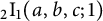 ${}_2\mathrm {I}_1 (a,b,c;1)$
, while the integral (9.22) reduces to
 ${}_2\mathrm {I}_1 (k-\alpha _2,k-\alpha _4,2k;1)$
in (9.23), which yields the desired result.
To estimate the second integral in (9.20), we again use (4.14) and (4.12). Consequently,
 $$ \begin{align} & \int_0^{\infty}\eta(x)\Phi_k\left(\frac{x}{1+x};\alpha_1,\alpha_2\right)(1+x)^{\alpha_1/2-\alpha_2/2}x^{-1-\alpha_4}dx \nonumber\\ &\quad = (-1)^k(2\pi)^{\alpha_1+\alpha_2} \frac{1}{2\pi i}\int_{(\sigma)}\Gamma(k,\alpha_1,\alpha_2;s)\sin\left(\pi\frac{s+\alpha_1+\alpha_2}{2}\right) \nonumber\\ &\qquad \times \int_0^{\infty}\eta(x)x^{-1/2-\alpha_4-\sigma}(1+x)^{-1/2+\alpha_1+\sigma}(1+1/x)^{iy}dxds, \end{align} $$
where
 $s/2=\sigma +iy$
. Integrating by parts A-times the integral over x, one has
 $$ \begin{align} \int_0^{\infty}\eta(x)x^{-1/2-\alpha_4-\sigma}(1+x)^{-1/2+\alpha_1+\sigma}(1+1/x)^{iy}dx\ll\frac{1}{(1+|y|)^A}. \end{align} $$
Moving the line of integration in (9.24) to
 $\Re {s}=-1/2$
, and applying (9.25) and (2.11) to estimate the Gamma factors, we infer
 $$ \begin{align} \int_0^{\infty}\eta(x)\Phi_k\left(\frac{x}{1+x};\alpha_1,\alpha_2\right)(1+x)^{\alpha_1/2-\alpha_2/2}x^{-1-\alpha_4}dx\ll \frac{1}{k^2}. \end{align} $$
Lemma 9.5 The following asymptotic formula holds:
 $$ \begin{align} &\int_0^{\infty}W_{2,1}(x)(1+x)^{\alpha_1-\alpha_2}dx \nonumber\\ &\quad =2(2\pi)^{\alpha_1-\alpha_2-2\alpha_3}X_k(\alpha_2)X_k(\alpha_3) \Gamma(\alpha_3-\alpha_1)\Gamma(\alpha_3+\alpha_2) \nonumber\\ &\qquad \times \cos\pi\frac{\alpha_1+\alpha_2}{2}+O(k^{-2}). \end{align} $$
Proof According to (6.17), one has
 $$ \begin{align} &\int_0^{\infty}W_{2,1}(x)(1+x)^{\alpha_1-\alpha_2}dx \nonumber\\ &\quad = \int_0^{\infty}\eta(1/x)\Phi_k\left(\frac{x}{1+x};\alpha_1,\alpha_2\right)(1+x)^{\alpha_1/2-\alpha_2/2}x^{-1-\alpha_3}dx. \end{align} $$
Therefore, changing
 $\alpha _4$
in (9.20) by
 $\alpha _3$
, we recover (9.28). Further, making the same change in (9.19), we obtain (9.27).
Lemma 9.6 The following asymptotic formula holds:
 $$ \begin{align} &\int_0^{\infty}W_{2,1}(x)x^{\alpha_3-\alpha_4}dx \nonumber\\ & \quad = 2(2\pi)^{-\alpha_1+\alpha_2-2\alpha_4}X_k(\alpha_1)X_k(\alpha_4) \Gamma(\alpha_4+\alpha_1)\Gamma(\alpha_4-\alpha_2)\cos\pi\frac{\alpha_1+\alpha_2}{2} \nonumber\\ &\qquad +O(k^{-2}). \end{align} $$
Proof Applying (6.17), one has
 $$ \begin{align} \int_0^{\infty}W_{2,1}(x)x^{\alpha_3-\alpha_4}dx= \int_0^{\infty}\eta(1/x)\Phi_k\left(\frac{x}{1+x};\alpha_1,\alpha_2\right)(1+x)^{-\alpha_1/2+\alpha_2/2}x^{-1-\alpha_4}dx. \end{align} $$
Note that (3.8) yields the identity
 $\Phi _k\left (y;\alpha _1,\alpha _2\right )=\Phi _k\left (y;\alpha _2,\alpha _1\right )$
. Therefore, changing
 $\alpha _1\leftrightarrow \alpha _2$
in (9.20), we obtain (9.30). Further, making the same change in (9.19), we recover (9.29).
Lemma 9.7 The following asymptotic formula holds:
 $$ \begin{align} &\int_0^{\infty}W_{2,1}(x)dx \nonumber\\ &\quad = 2(2\pi)^{-\alpha_1+\alpha_2-2\alpha_3}X_k(\alpha_1)X_k(\alpha_3) \Gamma(\alpha_3+\alpha_1)\Gamma(\alpha_3-\alpha_2)\cos\pi&\frac{\alpha_1+\alpha_2}{2} \nonumber\\ &\qquad +O(k^{-2}). \end{align} $$
Proof According to (6.17), one has
 $$ \begin{align} \int_0^{\infty}W_{2,1}(x)dx= \int_0^{\infty}\eta(1/x)\Phi_k\left(\frac{x}{1+x};\alpha_1,\alpha_2\right)(1+x)^{-\alpha_1/2+\alpha_2/2}x^{-1-\alpha_3}dx. \end{align} $$
Therefore, changing
 $\alpha _4$
in (9.30) by
 $\alpha _3$
, we recover (9.32). Making the same change in (9.29), we obtain (9.31).
Combining Lemmas 9.3–9.7, we finally prove the following identity.
Lemma 9.8 One has
 $$ \begin{align} \mathcal{U}(\bar{\alpha};W_{2,1})=MU_{2,1}(\bar{\alpha}), \end{align} $$
where
 $MU_{2,1}(\bar {\alpha })$
is defined by (9.5).
Proof Substituting (9.19), (9.27), (9.29), and (9.31) into (9.16) and using (2.3), we show that (9.5) holds.
The region (9.8) does not contain the most interesting points
 $\Re {\alpha _j}=0$
. In fact, the only obstacle in proving the analytic continuation for (9.9) is the term
 $\mathcal {E}_c(\bar {\alpha };W_{2,1})$
. In order to deal with this term, it is required to compute the sum
 $$ \begin{align} \widehat{W}_{2,1}^{+}(\alpha_3-\alpha_4,\alpha_1-\alpha_2;-i\xi)+\widehat{W}_{2,1}^{-}(\alpha_3-\alpha_4,\alpha_1-\alpha_2;-i\xi) \end{align} $$
at several special points
 $\xi .$
Lemma 9.9 For
 $|\alpha _j|\ll \epsilon $
and
 $\xi _1=\frac {1-\alpha _1-\alpha _2-\alpha _3-\alpha _4}{2}$
, one has
 $$ \begin{align} & \widehat{W}_{2,1}^{+}(\alpha_3-\alpha_4,\alpha_1-\alpha_2;-i\xi_1)+\widehat{W}_{2,1}^{-}(\alpha_3-\alpha_4,\alpha_1-\alpha_2;-i\xi_1) \nonumber\\ &\quad =\frac{\pi}{2}(2\pi)^{-\alpha_1+\alpha_2}X_k(\alpha_1) \Gamma(\alpha_2+\alpha_3)\Gamma(\alpha_2+\alpha_4)\Gamma(\alpha_3+\alpha_4) \frac{\Gamma(k-\alpha_2-\alpha_3-\alpha_4)}{\Gamma(k+\alpha_2+\alpha_3+\alpha_4)} \nonumber\\ &\qquad\times \frac{\cos\pi\frac{\alpha_3+\alpha_4+2\alpha_2}{2}+\cos\pi\frac{\alpha_3-\alpha_4}{2}}{\cos\pi\frac{\alpha_1+\alpha_2+\alpha_3+\alpha_4}{2}} \cos\pi\frac{\alpha_1+\alpha_2}{2}+O\left(\frac{1}{k^{2-\epsilon}}\right). \end{align} $$
Proof It follows from (5.12), (5.13), and (6.17) that
 $$ \begin{align} & \widehat{W}_{2,1}^{+}(\alpha_3-\alpha_4,\alpha_1-\alpha_2;-i\xi_1)+\widehat{W}_{2,1}^{-}(\alpha_3-\alpha_4,\alpha_1-\alpha_2;-i\xi_1) \nonumber\\ & \quad =\frac{\pi}{4}\frac{\cos\pi\frac{2\alpha_1+\alpha_3+\alpha_4}{2}-\cos\pi\frac{\alpha_3-\alpha_4}{2}}{\cos\pi\frac{\alpha_1+\alpha_2+\alpha_3+\alpha_4}{2}} \int_{0}^{\infty} \eta(1/y)\Phi_k\left(\frac{y}{1+y};\alpha_1,\alpha_2\right) \frac{y^{-2+\alpha_1}}{(1+y)^{\alpha_1/2-\alpha_2/2}} \nonumber\\ & \qquad \times {}_2\mathrm{I}_1 \left(1-\alpha_1-\alpha_4,1-\alpha_1-\alpha_3,2-\alpha_1-\alpha_2-\alpha_3-\alpha_4;\frac{-1}{y}\right)dy \nonumber\\ & \qquad + \frac{\pi}{4}\frac{\cos\pi\frac{2\alpha_2+\alpha_3+\alpha_4}{2}+\cos\pi\frac{\alpha_3-\alpha_4}{2}}{\cos\pi\frac{\alpha_1+\alpha_2+\alpha_3+\alpha_4}{2}} \int_{0}^{\infty} \eta(1/y)\Phi_k\left(\frac{y}{1+y};\alpha_1,\alpha_2\right) \nonumber\\ & \qquad \times\frac{y^{-1-\alpha_2-\alpha_3-\alpha_4}}{(1+y)^{\alpha_1/2-\alpha_2/2}} {}_2\mathrm{I}_1 \left(\alpha_2+\alpha_3,\alpha_2+\alpha_4,\alpha_1+\alpha_2+\alpha_3+\alpha_4;\frac{-1}{y}\right)dy. \end{align} $$
Let us first consider the second integral in (9.36). Using (2.15), it can be further split into the sum of two integrals:

Now, we compute the first integral in (9.37). Arguing in the same way as in Lemma 9.4, we obtain
 $$ \begin{align} & \frac{\Gamma(\alpha_2+\alpha_3)\Gamma(\alpha_2+\alpha_4)}{\Gamma(\alpha_1+\alpha_2+\alpha_3+\alpha_4)} \int_{0}^{\infty} \eta(1/y)\Phi_k\left(\frac{y}{1+y};\alpha_1,\alpha_2\right) \frac{y^{-1-\alpha_2-\alpha_3-\alpha_4}}{(1+y)^{\alpha_1/2-\alpha_2/2}}dy \nonumber\\ & \quad =2(2\pi)^{\alpha_1+\alpha_2}\cos\pi\frac{\alpha_1+\alpha_2}{2} \Gamma(\alpha_2+\alpha_3)\Gamma(\alpha_2+\alpha_4)\Gamma(\alpha_3+\alpha_4) \nonumber\\ & \qquad \times\frac{\Gamma(k-\alpha_2-\alpha_3-\alpha_4)\Gamma(k-\alpha_1)}{\Gamma(k+\alpha_2+\alpha_3+\alpha_4)\Gamma(k+\alpha_1)}+ O\left(\frac{1}{k^2}\right). \end{align} $$
To estimate the first integral in (9.36) and the second one in (9.37), we make the change of variable
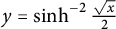 $y=\sinh ^{-2}\frac {\sqrt {x}}{2}$
and apply (4.25). The integral over
 $x>k^{\epsilon -2}$
is negligible since the K-Bessel function in (4.25) decays exponentially. Using the estimate
 $K_{\nu }(x)\ll x^{-|\Re {\nu }|}$
(see [Reference Olver, Lozier, Boisvert and Clarke25, 10.27.2, 10.30.2]), the remaining integral over
 $(0,k^{\epsilon -2})$
is bounded by
 $k^{\epsilon -2}$
.
Lemma 9.10 For
 $|\alpha _j|\ll \epsilon $
and
 $\xi _2=\frac {1+\alpha _1+\alpha _2-\alpha _3-\alpha _4}{2}$
, one has
 $$ \begin{align} & \widehat{W}_{2,1}^{+}(\alpha_3-\alpha_4,\alpha_1-\alpha_2;-i\xi_2)+\widehat{W}_{2,1}^{-}(\alpha_3-\alpha_4,\alpha_1-\alpha_2;-i\xi_2) \nonumber\\ & \quad =\frac{\pi}{2}(2\pi)^{-\alpha_1+\alpha_2}X_k(\alpha_1) \Gamma(\alpha_3+\alpha_4)\Gamma(\alpha_3-\alpha_1)\Gamma(\alpha_4-\alpha_1) \frac{\Gamma(k+\alpha_1-\alpha_3-\alpha_4)}{\Gamma(k-\alpha_1+\alpha_3+\alpha_4)} \nonumber\\ & \qquad \times \frac{\cos\pi\frac{\alpha_3+\alpha_4-2\alpha_2}{2}+\cos\pi\frac{\alpha_3-\alpha_4}{2}}{\cos\pi\frac{\alpha_1+\alpha_2-\alpha_3-\alpha_4}{2}} \cos\pi\frac{\alpha_1+\alpha_2}{2}+O\left(\frac{1}{k^{2-\epsilon}}\right). \end{align} $$
Proof It follows from (5.12), (5.13), and (6.17) that
 $$ \begin{align} &\widehat{W}_{2,1}^{+}(\alpha_3-\alpha_4,\alpha_1-\alpha_2;-i\xi_2)+\widehat{W}_{2,1}^{-}(\alpha_3-\alpha_4,\alpha_1-\alpha_2;-i\xi_2) = \nonumber\\ & \frac{\pi}{4}\frac{\cos\pi\frac{-2\alpha_2+\alpha_3+\alpha_4}{2}-\cos\pi\frac{\alpha_3-\alpha_4}{2}}{\cos\pi\frac{\alpha_1+\alpha_2-\alpha_3-\alpha_4}{2}} \int_{0}^{\infty} \eta(1/y)\Phi_k\left(\frac{y}{1+y};\alpha_1,\alpha_2\right) \frac{y^{-2-\alpha_2}}{(1+y)^{\alpha_1/2-\alpha_2/2}} \nonumber\\ & \times {}_2\mathrm{I}_1 \left(1+\alpha_2-\alpha_4,1+\alpha_2-\alpha_3,2+\alpha_1+\alpha_2-\alpha_3-\alpha_4;\frac{-1}{y}\right)dy \nonumber\\ & + \frac{\pi}{4}\frac{\cos\pi\frac{-2\alpha_1+\alpha_3+\alpha_4}{2}+\cos\pi\frac{\alpha_3-\alpha_4}{2}}{\cos\pi\frac{\alpha_1+\alpha_2-\alpha_3-\alpha_4}{2}} \int_{0}^{\infty} \eta(1/y)\Phi_k\left(\frac{y}{1+y};\alpha_1,\alpha_2\right) \frac{y^{-1+\alpha_1-\alpha_3-\alpha_4}}{(1+y)^{\alpha_1/2-\alpha_2/2}} \nonumber\\ & \times {}_2\mathrm{I}_1 \left(\alpha_3-\alpha_1,\alpha_4-\alpha_1,-\alpha_1-\alpha_2+\alpha_3+\alpha_4;\frac{-1}{y}\right)dy. \end{align} $$
Now, arguing in the same way as in Lemma 9.9, one can prove (9.39). Nevertheless, there is a simpler way to obtain (9.39), as we now show. Applying [Reference Olver, Lozier, Boisvert and Clarke25, 15.8.1], one has
 $$ \begin{align} X_k(\alpha_1)X_k(\alpha_2)\Phi_k\left(x;-\alpha_2,-\alpha_1\right)=\Phi_k\left(x;\alpha_1,\alpha_2\right). \end{align} $$
Therefore, making the change
 $\alpha _1\rightarrow -\alpha _2$
,
 $\alpha _2\rightarrow -\alpha _1$
in (9.36) and multiplying the result by
 $X_k(\alpha _1)X_k(\alpha _2)$
, we show that (9.40) holds. Hence, to prove (9.39), it is only required to perform this change of variables in (9.35) and multiply the result by
 $X_k(\alpha _1)X_k(\alpha _2)$
.
Now, we are ready to provide an analytic continuation for
 $\mathcal {E}_c(\bar {\alpha };W_{2,1})$
in the lemma below.
Lemma 9.11 For
 $|\alpha _j|\ll \epsilon ,$
one has
 $$ \begin{align} \mathcal{E}_{c}(\bar{\alpha};W_{2,1})=\mathbf{S}_{2,1}(\bar{\alpha})+T_{c}^{2}(\bar{\alpha}), \end{align} $$
where
 $\mathbf {S}_{2,1}(\bar {\alpha })$
and
 $T_{c}^{2}(\bar {\alpha })$
are defined by (9.6) and (9.3), respectively.
Proof Arguing in the same way as in Lemma 7.11, we obtain (9.6) with
 $$ \begin{align} \mathbf{S}_{2,1}(\bar{\alpha})= 8(2\pi)^{\alpha_1-\alpha_2-1}\left(R_{2,1}(\xi_1)+R_{2,1}(\xi_2)\right), \end{align} $$
 $$ \begin{align} R_{2,1}(\xi_1) &= \zeta_7(-\alpha_1,-\alpha_2,-\alpha_3,-\alpha_4)\mathcal{D}(\alpha_2+\alpha_3)\mathcal{D}(\alpha_2+\alpha_4)\mathcal{D}(\alpha_3+\alpha_4) \nonumber\\ & \quad \times \left(\widehat{W}_{2,1}^{+}(\alpha_3-\alpha_4,\alpha_1-\alpha_2;-i\xi_1)+\widehat{W}_{2,1}^{-}(\alpha_3+\alpha_4,\alpha_1-\alpha_2;-i\xi_1)\right), \end{align} $$
 $$ \begin{align} R_{2,1}(\xi_2) &= \zeta_7(\alpha_1,\alpha_2,-\alpha_3,-\alpha_4)\mathcal{D}(\alpha_4-\alpha_1)\mathcal{D}(\alpha_3-\alpha_1)\mathcal{D}(\alpha_3+\alpha_4) \nonumber\\ & \quad \times \left(\widehat{W}_{2,1}^{+}(\alpha_3-\alpha_4,\alpha_1-\alpha_2;-i\xi_2)+\widehat{W}_{2,1}^{-}(\alpha_3-\alpha_4,\alpha_1-\alpha_2;-i\xi_2)\right), \end{align} $$
where
 $$ \begin{align} \xi_1=\frac{1-\alpha_1-\alpha_2-\alpha_3-\alpha_4}{2},\quad \xi_2=\frac{1+\alpha_1+\alpha_2-\alpha_3-\alpha_4}{2}. \end{align} $$
Using (1.5) and (2.12), one has
 $$ \begin{align} \frac{\Gamma(k-\alpha_2-\alpha_3-\alpha_4)}{\Gamma(k+\alpha_2+\alpha_3+\alpha_4)}=(2\pi)^{-2\alpha_2-2\alpha_3-2\alpha_4} X_{k}(\alpha_2)X_{k}(\alpha_3)X_{k}(\alpha_4)\left(1+O(k^{-1})\right), \end{align} $$
 $$ \begin{align} \frac{\Gamma(k+\alpha_1-\alpha_3-\alpha_4)}{\Gamma(k-\alpha_1+\alpha_3+\alpha_4)}=(2\pi)^{2\alpha_1-2\alpha_3-2\alpha_4} \frac{X_{k}(\alpha_3)X_{k}(\alpha_4)}{X_{k}(\alpha_1)}\left(1+O(k^{-1})\right). \end{align} $$
Substituting (9.35) into (9.44) and using (9.47) and (2.3), we show that
 $$ \begin{align} & 8(2\pi)^{\alpha_1-\alpha_2-1} R_{2,1}(\xi_1) \nonumber\\ & \quad = \mathcal{C}(-\alpha_1,-\alpha_2,-\alpha_3,-\alpha_4)\zeta_7(-\alpha_1,-\alpha_2,-\alpha_3,-\alpha_4) \nonumber\\ & \qquad \times \frac{\cos\pi\frac{\alpha_3+\alpha_4+2\alpha_2}{2}+\cos\pi\frac{\alpha_3-\alpha_4}{2}} {4\cos\pi\frac{\alpha_2+\alpha_3}{2}\cos\pi\frac{\alpha_2+\alpha_4}{2}\cos\pi\frac{\alpha_3+\alpha_4}{2}} \frac{\cos\pi\frac{\alpha_1+\alpha_2}{2}}{\cos\pi\frac{\alpha_1+\alpha_2+\alpha_3+\alpha_4}{2}} +O\left(\frac{1}{k^{2-\epsilon}}\right). \end{align} $$
Substituting (9.39) into (9.45) and applying (9.48) and (2.3), we conclude that
 $$ \begin{align} & 8(2\pi)^{\alpha_1-\alpha_2-1} R_{2,1}(\xi_2) \nonumber\\ & \quad = \mathcal{C}(\alpha_1,\alpha_2,-\alpha_3,-\alpha_4)\zeta_7(\alpha_1,\alpha_2,-\alpha_3,-\alpha_4) \nonumber\\ & \qquad \times \frac{\cos\pi\frac{\alpha_3+\alpha_4-2\alpha_1}{2}+\cos\pi\frac{\alpha_3-\alpha_4}{2}} {4\cos\pi\frac{\alpha_3-\alpha_1}{2}\cos\pi\frac{\alpha_4-\alpha_1}{2}\cos\pi\frac{\alpha_3+\alpha_4}{2}} \frac{\cos\pi\frac{\alpha_1+\alpha_2}{2}}{\cos\pi\frac{\alpha_1+\alpha_2-\alpha_3-\alpha_4}{2}} +O\left(\frac{1}{k^{2-\epsilon}}\right). \end{align} $$
Substituting (9.49) and (9.50) into (9.43) and using [Reference Olver, Lozier, Boisvert and Clarke25, 4.21.8], we prove the lemma.
10 Analysis of
$\mathcal {TD}^{(2,2)}$

In this section, we show that the term
 $\mathcal {TD}^{(2,2)}(\bar {\alpha })$
does not contain any part of the main term of the fourth moment. More precisely, we prove that this term is negligible.
Similarly to other cases, applying Theorem 5.1 to study the sum (6.18), one has the following decomposition:
 $$ \begin{align} \mathcal{TD}^{(2,2)}(\bar{\alpha})=\mathcal{U}(\bar{\alpha};W_{2,2})+\mathcal{E}_h(\bar{\alpha};W_{2,2})+\mathcal{E}_d(\bar{\alpha};W_{2,2})+\mathcal{E}_c(\bar{\alpha};W_{2,2}). \end{align} $$
The main term
 $\mathcal {U}(\bar {\alpha };W_{2,2})$
of
 $\mathcal {TD}^{(2,2)}(\bar {\alpha })$
has the same structure as
 $\mathcal {U}(\bar {\alpha };W_{2,1})$
, see (9.16). It follows from (6.19) and (4.41) that
 $$ \begin{align} W_{2,2}(\bar{\alpha};x)\ll \frac{\eta(1/x)e^{-(2k-1)\log(\sqrt{1+x}+\sqrt{x})}}{(1+x)^{1/4+\Re{\alpha_1}/2-\Re{\alpha_2}/2}x^{1/4+\Re{\alpha_1}/2+\Re{\alpha_2}/2}k^{1/2+\Re{\alpha_1}+\Re{\alpha_2}}}. \end{align} $$
Hence, this function is negligible. Therefore, all integrals of the form like in (9.16) are negligible, and therefore,
 $\mathcal {U}(\bar {\alpha };W_{2,2})$
is negligible too. The same is true for the residue contribution
 $\mathbf {S}_{2,2}(\bar {\alpha })$
arising after analytic continuation of
 $\mathcal {E}_c(\bar {\alpha };W_{2,2})$
. Therefore, we are left to estimate
 $\mathcal {E}_{\ast }(\bar {\alpha };W_{2,2})$
for
 $\ast \in \{h,d,c\}$
.
The term
 $\mathcal {E}_{h}(\bar {\alpha };W_{2,2})$
is also negligible. This follows from the integral representation (5.23) and the estimates (4.41), (10.2) since
 $W_{2,2}(y)=0$
unless
 $y>x_0$
.
The case of
 $\mathcal {E}_{d}(\bar {\alpha };W_{2,2})$
can be treated along the line of the proof of Lemma 7.2 with the help of (10.2). After integration by parts, we obtain derivatives of the function
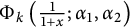 $\Phi _k\left (\frac {1}{1+x};\alpha _1,\alpha _2\right )$
. Being a hypergeometric function, it satisfies a second-order differential equation with coefficients depending on k polynomially. Therefore, all derivatives of
 $\Phi _k$
could be replaced by
 $\Phi _k$
and
 $\Phi ^{\prime }_k$
at the cost of the error
 $k^{A}$
. To get rid of
 $\Phi ^{\prime }_k$
, we integrate by parts once again. Finally, using (10.2), which shows the exponential decay in k, we prove the estimate
 $\mathcal {E}_{d}(\bar {\alpha };W_{2,2})\ll k^{-A}.$
The same arguments lead to
 $\mathcal {E}_{c}(\bar {\alpha };W_{2,2})\ll k^{-A}.$
11 Analysis of
$\mathcal {TD}^{(3)}$

Lemma 11.1 For
 $|\alpha _j|\ll \epsilon ,$
one has
 $$ \begin{align} \mathcal{TD}^{(3)}(\bar{\alpha}) & =MU_3(\bar{\alpha})+\mathbf{S}_3(\bar{\alpha}) \nonumber\\ & \quad + (-1)^kX_k(\alpha_2)\left(T_{h}^{2}+T_{d}^2+T_c^{2}\right)(\alpha_1,-\alpha_2,\alpha_3,\alpha_4)+O(k^{\epsilon-2}), \end{align} $$
where
 $T_{h}^{2}(\bar {\alpha })$
,
 $T_{d}^{2}(\bar {\alpha }),$
and
 $T_{c}^{2}(\bar {\alpha })$
are given by (9.2), (9.1), and (9.3), respectively, and
 $$ \begin{align} MU_3(\bar{\alpha})&:= \mathcal{C}(\alpha_1,\alpha_2,\alpha_3,-\alpha_4)\zeta_7(\alpha_1,\alpha_2,\alpha_3,-\alpha_4) \frac{\cos\pi\frac{\alpha_1-\alpha_2}{2}}{2\cos\pi\frac{\alpha_4-\alpha_2}{2}\cos\pi\frac{\alpha_4-\alpha_1}{2}} \nonumber\\ &\quad + \mathcal{C}(\alpha_1,\alpha_2,-\alpha_3,\alpha_4)\zeta_7(\alpha_1,\alpha_2,-\alpha_3,\alpha_4) \frac{\cos\pi\frac{\alpha_1-\alpha_2}{2}}{2\cos\pi\frac{\alpha_3-\alpha_1}{2}\cos\pi\frac{\alpha_3-\alpha_2}{2}} \nonumber\\ &\quad + \mathcal{C}(-\alpha_1,-\alpha_2,\alpha_3,-\alpha_4)\zeta_7(-\alpha_1,-\alpha_2,\alpha_3,-\alpha_4) \frac{\cos\pi\frac{\alpha_1-\alpha_2}{2}}{2\cos\pi\frac{\alpha_4+\alpha_1}{2}\cos\pi\frac{\alpha_4+\alpha_2}{2}} \nonumber\\ &\quad + \mathcal{C}(-\alpha_1,-\alpha_2,-\alpha_3,\alpha_4)\zeta_7(-\alpha_1,-\alpha_2,-\alpha_3,\alpha_4) \frac{\cos\pi\frac{\alpha_1-\alpha_2}{2}}{2\cos\pi\frac{\alpha_3+\alpha_1}{2}\cos\pi\frac{\alpha_3+\alpha_2}{2}}, \end{align} $$
 $$ \begin{align} \mathbf{S}_{3}(\bar{\alpha}) &:= \mathcal{C}(-\alpha_1,\alpha_2,-\alpha_3,-\alpha_4)\zeta_7(-\alpha_1,\alpha_2,-\alpha_3,-\alpha_4) \frac{\cos\pi\frac{\alpha_1-\alpha_2}{2}}{2\cos\pi\frac{\alpha_4+\alpha_3}{2}\cos\pi\frac{\alpha_1-\alpha_2+\alpha_3+\alpha_4}{2}} \nonumber\\ &\quad + \mathcal{C}(\alpha_1,-\alpha_2,-\alpha_3,-\alpha_4)\zeta_7(\alpha_1,-\alpha_2,-\alpha_3,-\alpha_4) \frac{\cos\pi\frac{\alpha_1-\alpha_2}{2}}{2\cos\pi\frac{\alpha_4+\alpha_3}{2}\cos\pi\frac{\alpha_1-\alpha_2-\alpha_3-\alpha_4}{2}}. \end{align} $$
Proof It follows from (6.4) and (3.5) that
 $$ \begin{align} \mathcal{TD}^{(3)}(\alpha_1,\alpha_2,\alpha_3,\alpha_4)= (-1)^kX_k(\alpha_2)\mathcal{TD}^{(2)}(\alpha_1,-\alpha_2,\alpha_3,\alpha_4). \end{align} $$
Therefore, using (9.9), one has
 $$ \begin{align} \mathcal{TD}^{(3)}(\bar{\alpha})=\mathcal{U}_3(\bar{\alpha})+\mathbf{S}_3(\bar{\alpha})\end{align} $$
 $$ \begin{align} + (-1)^kX_k(\alpha_2)\left(\mathcal{E}_h+\mathcal{E}_d+\mathcal{E}_c^{(0)}\right)(\alpha_1,-\alpha_2,\alpha_3,\alpha_4;W_{2,1})+O(k^{\epsilon-2}), \end{align} $$
where
 $$ \begin{align} \mathcal{U}_3(\bar{\alpha})=(-1)^kX_k(\alpha_2)\mathcal{U}(\alpha_1,-\alpha_2,\alpha_3,\alpha_4;W_{2,1}), \end{align} $$
and (see (9.42))
 $$ \begin{align} \mathbf{S}_3(\bar{\alpha})=(-1)^kX_k(\alpha_2)\mathbf{S}_{2,1}(\alpha_1,-\alpha_2,\alpha_3,\alpha_4). \end{align} $$
In the beginning of Section 8, it was shown that changing the sign of
 $\epsilon _2$
in
 $\mathcal {C}(\epsilon _1\alpha _1,\epsilon _2\alpha _2,\epsilon _3\alpha _3,\epsilon _4\alpha _4)$
and then multiplying by
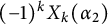 $(-1)^kX_k(\alpha _2)$
, we obtain
 $\mathcal {C}(\epsilon _1\alpha _1,-\epsilon _2\alpha _2,\epsilon _3\alpha _3,\epsilon _4\alpha _4)$
. Therefore, using (9.5), one has
 $\mathcal {U}_3(\bar {\alpha })=MU_{3}(\bar {\alpha })$
. Applying (9.6), we show that (11.3) holds.
12 Proof of Theorem 1.1
In order to prove the main theorem, we use the formula (6.4) for the fourth moment together with the decomposition (6.11) and Lemmas 7.1, 8.1, 9.1, and 11.1. Further, note that the contribution of the term
 $\mathcal {TD}^{(2,2)}(\bar {\alpha })$
to the fourth moment is negligible according to Section 10.
The final step is to rearrange slightly all main terms.
Summing (8.4) and (9.5) and using [Reference Olver, Lozier, Boisvert and Clarke25, 4.21.16], we infer
 $$ \begin{align} MU_{1,2}(\bar{\alpha})+MU_{2,1}(\bar{\alpha}) &= \mathcal{C}(\alpha_1,-\alpha_2,\alpha_3,-\alpha_4)\zeta_7(\alpha_1,-\alpha_2,\alpha_3,-\alpha_4) \nonumber\\ &\quad + \mathcal{C}(\alpha_1,-\alpha_2,-\alpha_3,\alpha_4)\zeta_7(\alpha_1,-\alpha_2,-\alpha_3,\alpha_4) \nonumber\\ &\quad + \mathcal{C}(-\alpha_1,\alpha_2,\alpha_3,-\alpha_4)\zeta_7(-\alpha_1,\alpha_2,\alpha_3,-\alpha_4) \nonumber\\ &\quad + \mathcal{C}(-\alpha_1,\alpha_2,-\alpha_3,\alpha_4)\zeta_7(-\alpha_1,\alpha_2,-\alpha_3,\alpha_4). \end{align} $$
Similarly, summing (8.5) and (9.6) and applying [Reference Olver, Lozier, Boisvert and Clarke25, 4.21.16], we prove that
 $$ \begin{align} \mathbf{S}_{1,2}(\bar{\alpha})+\mathbf{S}_{2,1}(\bar{\alpha}) &= \mathcal{C}(-\alpha_1,-\alpha_2,-\alpha_3,-\alpha_4)\zeta_7 (-\alpha_1,-\alpha_2,-\alpha_3,-\alpha_4) \nonumber\\ & \quad + \mathcal{C}(\alpha_1,\alpha_2,-\alpha_3,-\alpha_4)\zeta_7(\alpha_1,\alpha_2,-\alpha_3,-\alpha_4). \end{align} $$
Now, let us sum (7.5) and (11.2) with the help of [Reference Olver, Lozier, Boisvert and Clarke25, 4.21.16]. This gives
 $$ \begin{align} MU_{1,1}(\bar{\alpha})+MU_3(\bar{\alpha}) &= \mathcal{C}(\alpha_1,\alpha_2,\alpha_3,-\alpha_4)\zeta_7(\alpha_1,\alpha_2,\alpha_3,-\alpha_4) \nonumber\\ &\quad + \mathcal{C}(\alpha_1,\alpha_2,-\alpha_3,\alpha_4)\zeta_7(\alpha_1,\alpha_2,-\alpha_3,\alpha_4) \nonumber\\ &\quad + \mathcal{C}(-\alpha_1,-\alpha_2,\alpha_3,-\alpha_4)\zeta_7(-\alpha_1,-\alpha_2,\alpha_3,-\alpha_4) \nonumber\\ &\quad + \mathcal{C}(-\alpha_1,-\alpha_2,-\alpha_3,\alpha_4)\zeta_7(-\alpha_1,-\alpha_2,-\alpha_3,\alpha_4). \end{align} $$
Summing (7.6) and (11.3) and applying [Reference Olver, Lozier, Boisvert and Clarke25, 4.21.16], we conclude that
 $$ \begin{align} \mathbf{S}_{1,1}(\bar{\alpha})+\mathbf{S}_{3}(\bar{\alpha}) &= \mathcal{C}(-\alpha_1,\alpha_2,-\alpha_3,-\alpha_4)\zeta_7 (-\alpha_1,\alpha_2,-\alpha_3,-\alpha_4) \nonumber\\ &\quad + \mathcal{C}(\alpha_1,-\alpha_2,-\alpha_3,-\alpha_4)\zeta_7(\alpha_1,-\alpha_2,-\alpha_3,-\alpha_4). \end{align} $$
Finally, it follows from (1.2), (6.5), and (12.1)–(12.4) that
 $$ \begin{align} & \mathcal{MT}_{2,4}(\bar{\alpha})+MU_{1,2}(\bar{\alpha})+MU_{2,1}(\bar{\alpha})+\mathbf{S}_{1,2}(\bar{\alpha}) +\mathbf{S}_{2,1}(\bar{\alpha}) \nonumber\\ &\qquad + MU_{1,1}(\bar{\alpha})+MU_3(\bar{\alpha})+\mathbf{S}_{1,1}(\bar{\alpha})+\mathbf{S}_{3}(\bar{\alpha}) \nonumber\\ &\quad =\mathcal{MT}_4(\alpha_1,\alpha_2,\alpha_3,\alpha_4). \end{align} $$
A Appendix. Kuznetsov’s proof of Theorem 1.2
Let us take
 $\alpha _1=\alpha _2=\alpha _3=\alpha _4=0$
(consequently, we may delete dependence on
 $\alpha $
in all formulas) and try to estimate the right-hand side of (1.6). First, we show that the terms
 $\mathcal {E}_h(W_{1,1})$
and
 $\mathcal {E}_h(W_{2,1})$
are negligible. This follows from the result below.
Lemma A.1 For
 $m>2,$
the following estimate holds:
 $$ \begin{align} \widehat{W}_{1,1}(m)+\widehat{W}_{2,1}(m)\ll\frac{1}{k^2m^A}, \end{align} $$
and therefore,
 $$ \begin{align} T_{h}^{1}\ll\frac{1}{k^2},\quad T_{h}^{2}\ll\frac{1}{k^2}. \end{align} $$
Proof Let us start with estimating
 $\widehat {W}_{2,1}(m)$
. It follows from (5.23), (6.17), and (6.9) that
 $$ \begin{align} \widehat{W}_{2,1}(m) &\ll \int_{x_0}^{\infty}\frac{\eta(1/y)}{y}\Phi_k\left(\frac{y}{1+y}\right)\Phi_m \left(\frac{1}{1+y}\right)dy \nonumber\\ & \ll \int_{x_0/(1+x_0)}^{1}\frac{\eta(1/x-1)}{x(1-x)}\Phi_k\left(x\right)\Phi_m\left(1-x\right)dx. \end{align} $$
We split the integral into two: the first one over
 $x_0/(1+x_0)<x<1-k^{-\delta }$
and the second one over
 $1-k^{-\delta }<x<1$
with
 $1<\delta <2$
. The first integral is negligible by (4.42). To bound the second integral, we apply (4.42) and (4.43). This yields
 $$ \begin{align} \widehat{W}_{2,1}(m)\ll\frac{1}{(km)^{A}}+\frac{1}{m^Ak^{\delta(m-1)}}. \end{align} $$
The case of
 $\widehat {W}_{1,1}(m)$
is slightly more complicated. It follows from (5.23), (6.13), and (6.9) that
 $$ \begin{align} \widehat{W}_{1,1}(m) &\ll \int_{x_0}^{\infty}\frac{\eta(1/y)}{1+y}\phi_k\left(\frac{1}{1+y}\right)\Phi_m\left(\frac{1}{1+y}\right)dy \nonumber\\ &\ll \int_{0}^{(1+x_0)^{-1}}\eta\left(\frac{x}{1-x}\right)\phi_k\left(x\right)\Phi_m\left(x\right)\frac{dx}{x}. \end{align} $$
Using (6.9), we smoothly split the last integral into two: the first one over
 $0<x\ll k^{-\delta }$
and the second over
 $k^{-\delta }\ll x<1/(1+x_0)$
with some
 $1<\delta <2$
. As a result,
 $$ \begin{align} \widehat{W}_{1,1}(m)\ll\widehat{W}_{1,1,1}(m)+\widehat{W}_{1,1,2}(m), \end{align} $$
 $$ \begin{align} \widehat{W}_{1,1,1}(m)=\int_{0}^{(1+x_0)^{-1}}\eta\left(\frac{x}{k^{-\delta}}\right)\eta\left(\frac{x}{1-x}\right)\phi_k\left(x\right)\Phi_m\left(x\right)\frac{dx}{x}, \end{align} $$
 $$ \begin{align} \widehat{W}_{1,1,2}(m)=\int_{0}^{(1+x_0)^{-1}}\eta\left(\frac{k^{-\delta}}{x}\right)\eta\left(\frac{x}{1-x}\right)\phi_k\left(x\right)\Phi_m\left(x\right)\frac{dx}{x}. \end{align} $$
It follows from (6.9) that, as
 $k\rightarrow +\infty ,$
one has
 $\eta \left (\frac {x}{1-x}\right )=1$
when
 $\eta \left (\frac {x}{k^{-\delta }}\right )\neq 0$
. Using (4.42) and Lemma 4.5, we estimate
 $\widehat {W}_{1,1,1}(m)$
trivially as
 $$ \begin{align} \widehat{W}_{1,1,1}(m)=\int_{0}^{1}\eta\left(\frac{x}{k^{-\delta}}\right)\phi_k\left(x\right)\Phi_m\left(x\right)\frac{dx}{x}\ll\frac{1}{m^Ak^{\delta(m-1)}}. \end{align} $$
Now, let us estimate the integral
 $\widehat {W}_{1,1,2}(m)$
. Define
 $$ \begin{align} \mathbf{y}_k(x)=\sqrt{x(1-x)}\phi_k(x),\quad \mathcal{Y}_m(x)=\sqrt{1-x}\Phi_m(x). \end{align} $$
These functions satisfy the differential equations (see [Reference Balkanova and Frolenkov4, Corollary 5.6, Lemma 5.15]):
 $$ \begin{align} \mathbf{y}_k"(x)+\left(\frac{1}{4x^2(1-x)^2}+\frac{k(k-1)}{x(1-x)} \right)\mathbf{y}_k(x)=0, \end{align} $$
 $$ \begin{align} \mathcal{Y}_m"(x)-\left(\frac{(m-1/2)^2}{x^2(1-x)}-\frac{1}{4x^2(1-x)^2}+\frac{1}{4x(1-x)} \right)\mathcal{Y}_m(x)=0. \end{align} $$
Using (A.11) and integrating by parts twice, we have
 $$ \begin{align} \widehat{W}_{1,1,2}(m)=\int_{0}^{(1+x_0)^{-1}}\frac{\partial^2}{\partial x^2}\left( \eta\left(\frac{k^{-\delta}}{x}\right) \eta\left(\frac{x}{1-x}\right)\frac{\mathcal{Y}_m\left(x\right)x^{1/2}(1-x)} {\left(\frac{1}{4}+k(k-1)x(1-x) \right)} \right)\mathbf{y}_k(x)dx. \end{align} $$
After lengthy but straightforward computations, it turns out that the largest contribution comes from the second derivative of
 $\mathcal {Y}_m(x)$
. Applying (A.12), followed by (4.42) and Lemma 4.5, one has
 $$ \begin{align} \widehat{W}_{1,1,2}(m) &\ll\int_{0}^{(1+x_0)^{-1}} \eta\left(\frac{k^{-\delta}}{x}\right) \eta\left(\frac{x}{1-x}\right) \frac{\mathcal{Y}_m(x)\mathbf{y}_k(x)x^{1/2}(1-x)} {\left(\frac{1}{4}+k(k-1)x(1-x) \right)}\frac{(m-1/2)^2}{x^2(1-x)}dx \nonumber\\ &\ll \frac{m^2}{k^2}\int_{k^{-\delta}}^{(1+x_0)^{-1}}\frac{\phi_k(x)\Phi_m(x)}{x^2}dx\ll\frac{1}{k^2m^A}. \end{align} $$
Substituting (A.9) and (A.14) to (A.6), we show that
 $$ \begin{align} \widehat{W}_{1,1}(m)\ll\frac{1}{k^2m^{A}}+\frac{1}{m^Ak^{\delta(m-1)}}. \end{align} $$
The next step is to prove that the terms
 $T_{d}^{2}$
and
 $T_{c}^{2}$
are also small.
Lemma A.2 One has
 $$ \begin{align} \widehat{W}_{2,1}^{0}(ir)\ll\frac{1}{k^{1-\epsilon}r^{5/2}}, \end{align} $$
and therefore,
 $$ \begin{align} T_{d}^{2}+T_{c}^{2}\ll\frac{1}{k^{1-\epsilon}}. \end{align} $$
Proof Using (5.13) and (6.17) and making the change of variable
 $\frac {y}{1+y}=x$
, we obtain
 $$ \begin{align} \widehat{W}_{2,1}^{0}(ir) &= \int_{0}^{1} \eta\left(\frac{1-x}{x}\right)\Phi_k\left(x\right) \left(\frac{x}{1-x}\right)^{-1/2-ir} {}_2\mathrm{I}_1 \left(\frac{1}{2}+ir,\frac{1}{2}+ir,1+2ir;\frac{x-1}{x}\right) \nonumber\\ &\quad \times\frac{dx}{x(1-x)}. \end{align} $$
Now, we can replace
 ${}_2\mathrm {I}_1 \left (\cdot \right )$
in (A.18) by its asymptotic expansion given by (4.44). It is enough to investigate only the contribution of the main term:
 $$ \begin{align} {}_2\mathrm{I}_1 \left(\frac{1}{2}+ir,\frac{1}{2}+ir,1+2ir;\frac{-(1-x)}{x}\right)\sim\frac{(1-x)^{1/4}}{\sqrt{|r|+1}} \left(\frac{x}{1-x}\right)^{\frac{1}{4}+ir}\left(\frac{1+\sqrt{x}}{\sqrt{1-x}}\right)^{-2ir}, \end{align} $$
since all other terms are of the same shape and are smaller in absolute value. To estimate the contribution of the error term in (4.44), we also apply (4.42) and (4.43), thus obtaining
 $$ \begin{align} \frac{1}{(k|r|)^A}+\frac{1}{|r|^A} \int_{1-k^{-2+\epsilon}}^{1}\frac{dx}{(1-x)^{1/2-\epsilon}}\ll\frac{1}{k^{1-\epsilon}|r|^A}, \end{align} $$
which is better than (A.16). Using the notation (A.10), one has
 $$ \begin{align} \widehat{W}_{2,1}^{0}(ir)\ll\frac{1}{k^{1-\epsilon}|r|^A}+\frac{1}{\sqrt{|r|}} \int_{0}^{1} \eta\left(\frac{1-x}{x}\right)\frac{\mathcal{Y}_k\left(x\right)}{x^{5/4}(1-x)} \left(\frac{1+\sqrt{x}}{\sqrt{1-x}}\right)^{-2ir}dx. \end{align} $$
Integrating by parts twice, we infer
 $$ \begin{align} \widehat{W}_{2,1}^{0}(ir) &\ll\frac{1}{k^{1-\epsilon}|r|^A}+\frac{1}{|r|^{5/2}} \int_{0}^{1}\left(\frac{1+\sqrt{x}}{\sqrt{1-x}}\right)^{-2ir} \frac{\partial}{\partial x}\Big(\frac{\mathcal{Y}_k(x)(1-x)}{x^{1/4}}\frac{\partial}{\partial x}\eta\left(\frac{1-x}{x}\right) \nonumber\\ &\quad + \eta\left(\frac{1-x}{x}\right)\frac{\mathcal{Y}^{\prime}_k(x)(1-x)}{x^{1/4}}+ \eta\left(\frac{1-x}{x}\right)\frac{\mathcal{Y}_k(x)(1-x)}{x^{5/4}} \Big)dx. \end{align} $$
The derivative of
 $\eta \left (\frac {1-x}{x}\right )$
is nonzero only for
 $x_0/(1+x_0)<x<1/(1+x_0)$
, in which case
 $\mathcal {Y}_k(x)$
and its derivative are (4.42) negligible. Furthermore, all powers of x can be estimated by constants since we integrate over
 $x_0/(1+x_0)<x<1$
. Hence,
 $$ \begin{align} \widehat{W}_{2,1}^{0}(ir) &\ll\frac{1}{k^{1-\epsilon}|r|^A}+\frac{1}{|r|^{5/2}} \int_{0}^{1}\eta\left(\frac{1-x}{x}\right)\left(\frac{1+\sqrt{x}}{\sqrt{1-x}}\right)^{-2ir} \nonumber\\ & \quad\times \Big(\frac{\mathcal{Y}^{\prime\prime}_k(x)(1-x)}{x^{1/4}}+\frac{\mathcal{Y}^{\prime}_k(x)}{x^{1/4}}+\frac{\mathcal{Y}_k(x)}{x^{5/4}} \Big)dx. \end{align} $$
Consider the summand with
 $\mathcal {Y}^{\prime }_k(x)$
. Integrating by parts, we obtain that it is bounded by
 $$ \begin{align} & \frac{1}{|r|^{7/2}} \int_{0}^{1}\eta\left(\frac{1-x}{x}\right)\left(\frac{1+\sqrt{x}}{\sqrt{1-x}}\right)^{-2ir} \nonumber\\ &\quad \times \Big(\mathcal{Y}^{\prime\prime}_k(x)(1-x)x^{1/4}+\mathcal{Y}^{\prime}_k(x)x^{1/4}+\frac{\mathcal{Y}^{\prime}_k(x)(1-x)}{x^{3/4}} \Big)dx. \end{align} $$
Therefore,
 $$ \begin{align} \widehat{W}_{2,1}^{0}(ir) & \ll\frac{1}{k^{1-\epsilon}|r|^A}+\frac{1}{|r|^{5/2}} \int_{0}^{1}\eta\left(\frac{1-x}{x}\right)\left(\frac{1+\sqrt{x}}{\sqrt{1-x}}\right)^{-2ir} \nonumber\\ & \quad\times \Big(\frac{\mathcal{Y}^{\prime\prime}_k(x)(1-x)}{x^{1/4}}+\frac{\mathcal{Y}_k(x)}{x^{5/4}} \Big)dx \nonumber\\ &\quad \times +\frac{1}{|r|^{7/2}} \int_{0}^{1}\eta\left(\frac{1-x}{x}\right)\left(\frac{1+\sqrt{x}}{\sqrt{1-x}}\right)^{-2ir} \mathcal{Y}^{\prime}_k(x)x^{1/4}dx. \end{align} $$
In order to get rid of
 $\mathcal {Y}^{\prime }_k(x)$
, we integrate by parts once again
 $$ \begin{align} & \frac{1}{|r|^{7/2}} \int_{0}^{1}\eta\left(\frac{1-x}{x}\right)\left(\frac{1+\sqrt{x}}{\sqrt{1-x}}\right)^{-2ir} \mathcal{Y}^{\prime}_k(x)x^{1/4}dx \nonumber\\ & \quad\ll \frac{1}{|r|^{5/2}} \int_{0}^{1}\eta\left(\frac{1-x}{x}\right)\left(\frac{1+\sqrt{x}}{\sqrt{1-x}}\right)^{-2ir}\frac{\mathcal{Y}_k(x)}{x^{1/4}(1-x)}dx. \end{align} $$
Substituting (A.26) into (A.25), one has
 $$ \begin{align} \widehat{W}_{2,1}^{0}(ir) & \ll\frac{1}{k^{1-\epsilon}|r|^A}+\frac{1}{|r|^{5/2}} \int_{0}^{1}\eta\left(\frac{1-x}{x}\right) \left(\frac{1+\sqrt{x}}{\sqrt{1-x}}\right)^{-2ir} \nonumber\\ & \quad\times \Big(\frac{\mathcal{Y}^{\prime\prime}_k(x)(1-x)}{x^{1/4}}+\frac{\mathcal{Y}_k(x)}{x^{1/4}(1-x)} \Big)dx. \end{align} $$
Applying (A.12) to replace
 $\mathcal {Y}^{\prime \prime }_k(x)$
, we show that
 $$ \begin{align} \widehat{W}_{2,1}^{0}(ir) & \ll\frac{1}{k^{1-\epsilon}|r|^A} \nonumber\\ &\quad +\frac{1}{|r|^{5/2}} \int_{0}^{1}\eta\left(\frac{1-x}{x}\right)\left(\frac{1+\sqrt{x}}{\sqrt{1-x}}\right)^{-2ir} \Big(\frac{k^2\mathcal{Y}_k(x)}{x^{9/4}}+\frac{\mathcal{Y}_k(x)}{x^{9/4}(1-x)} \Big)dx. \end{align} $$
Finally, using (4.42) and (4.43), we prove (A.16).
In order to prove (A.17), we apply (A.16) together with the mean Lindelöf estimate (see [Reference Ivic15]):
 $$ \begin{align} \sum_{T<t_j<2T}\omega_jL_j(1/2)^4\ll T^{2+\epsilon}, \end{align} $$
and the upper bound on the eighth moment of the Riemann zeta function (see [Reference Ivic15, (4.3)]):
 $$ \begin{align} \int_T^{2T}|\zeta(1/2+it)|^8dt\ll T^{3/2+\epsilon}. \end{align} $$
The last estimate follows from the upper bound on the 12th moment due to Heath-Brown [Reference Heath-Brown12], the mean Lindelöf estimate on the fourth moment and the Cauchy–Schwartz inequality:
 $$ \begin{align} \int_T^{2T}|\zeta(1/2+it)|^8dt &\ll \left(\int_T^{2T}|\zeta(1/2+it)|^{12}dt\right)^{1/2} \left(\int_T^{2T}|\zeta(1/2+it)|^4dt\right)^{1/2} \nonumber\\ & \ll T^{3/2+\epsilon}.\\[-34pt]\nonumber \end{align} $$
We are left to investigate the behavior of
 $\widehat {W}_{1,1}(t)$
. This is the most important ingredient of the proof of Theorem 1.2. Let
 $u=k-1/2$
and for
 $r\le u,$
let
 $\xi _0$
be such that
 $$ \begin{align} \sin\xi_0=\frac{r}{u}. \end{align} $$
Lemma A.3 For
 $r\gg k^{1+\epsilon }$
, one has
 $$ \begin{align} \widehat{W}_{1,1}^{0}(ir)\ll\frac{1}{k(r/k)^A}. \end{align} $$
For
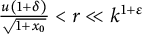 $\frac {u(1+\delta )}{\sqrt {1+x_0}}<r\ll k^{1+\epsilon }$
, one has
 $$ \begin{align} \widehat{W}_{1,1}^{0}(ir)\ll\frac{1}{k^A}. \end{align} $$
For
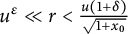 $u^{\epsilon }\ll r<\frac {u(1+\delta )}{\sqrt {1+x_0}}$
, one has
 $$ \begin{align} \widehat{W}_{1,1}^{0}(ir)= \frac{c_0(r)e^{iw(r,u)}}{\sqrt{ur}(u^2-r^2)^{1/4}}\eta\left(\frac{r^2}{u^2-r^2}\right)+O\left(\frac{1}{ur^{3/2}}\right), \end{align} $$
where
 $|c_0(r)|\ll 1$
and
 $$ \begin{align} w(r,u)=-2u\arcsin\frac{r}{u}+2r\log\frac{r}{u+\sqrt{u^2-r^2}}. \end{align} $$
Furthermore,
 $$ \begin{align} \widehat{W}_{1,1}^{0}(ir)\ll\frac{1}{k^{1/2}}. \end{align} $$
Proof Using (5.13) and (6.17) and making the change of variable
 $\frac {1}{1+y}=x$
, we obtain
 $$ \begin{align} \widehat{W}_{1,1}^{0}(ir) &= \int_{0}^{1} \eta\left(\frac{x}{1-x}\right)\phi_k\left(x\right) \left(\frac{x}{1-x}\right)^{ir} \nonumber\\ & \quad\times {}_2\mathrm{I}_1 \left(\frac{1}{2}+ir,\frac{1}{2}+ir,1+2ir;\frac{-x}{1-x}\right)\frac{dx}{\sqrt{x(1-x)}}. \end{align} $$
Estimating the integral trivially by absolute value with the use of Lemmas 4.6 and 4.9, we show that
 $\widehat {W}_{1,1}^{0}(ir)\ll k^{-1/2}$
, thus proving (A.37).
Next, we replace
 ${}_2\mathrm {I}_1 \left (\cdot \right )$
in (A.38) by its asymptotic expansion (4.44). Again it is enough to investigate only the contribution of the main term
 $$ \begin{align} {}_2\mathrm{I}_1 \left(\frac{1}{2}+ir,\frac{1}{2}+ir,1+2ir;\frac{-x}{1-x}\right)\sim \frac{(1-x)^{1/4}}{\sqrt{r}} \left(\frac{x}{1-x}\right)^{-ir}\left(\frac{1+\sqrt{1-x}}{\sqrt{x}}\right)^{-2ir}, \end{align} $$
since all other terms are of the same shape and are smaller in absolute value. To estimate the contribution of the error term in (4.44) to (A.38), we apply Lemma 4.6, getting
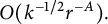 $O(k^{-1/2}r^{-A}).$
Substituting (A.39) into (A.38) and using the definition (A.10), we infer
 $$ \begin{align} \widehat{W}_{1,1}^{0}(ir)\ll k^{-1/2}r^{-A}+ \frac{1}{\sqrt{r}}\int_{0}^{1} \eta\left(\frac{x}{1-x}\right)\left(\frac{1+\sqrt{1-x}}{\sqrt{x}}\right)^{-2ir}\frac{\mathbf{y}_k(x)dx}{(1-x)^{3/4}x}. \end{align} $$
Integration by parts repeated n times yields the upper bound:
 $$ \begin{align} \widehat{W}_{1,1}^{0}(ir)\ll k^{-1/2}r^{-A}+ \frac{1}{r^{1/2+2n}}\int_{0}^{1} D^n\left(\eta\left(\frac{x}{1-x}\right)\frac{\mathbf{y}_k(x)}{(1-x)^{3/4}x}\right) \left(\frac{1+\sqrt{1-x}}{\sqrt{x}}\right)^{-2ir}dx, \end{align} $$
where
 $D(f(x))=\frac {\partial }{\partial x}(xf(x)\sqrt {1-x})$
. In order to study the integral above, we apply (A.11) in a way that avoids high derivatives of
 $\mathbf {y}_k(x)$
. More precisely, every time we obtain
 $\mathbf {y}_k"(x)$
, we replace it using (A.11) so that we finally get a combination of
 $\mathbf {y}_k(x)$
and
 $\mathbf {y}^{\prime }_k(x)$
. In order not to deal with
 $\mathbf {y}^{\prime }_k(x),$
we integrate by parts “back,” obtaining only
 $\mathbf {y}_k(x)$
. It turns out that the worst case scenario is when on each step of integration by parts, we take the derivative of
 $\mathbf {y}_k(x)$
and later replace
 $\mathbf {y}_k"(x)$
by
 $k^2\mathbf {y}_k(x)/(x(1-x))$
. In this case, we show that
 $$ \begin{align} \widehat{W}_{1,1}^{0}(ir) &\ll k^{-1/2}r^{-A}+ \frac{k^{2n}}{r^{1/2+2n}}\int_{0}^{1} \eta\left(\frac{x}{1-x}\right)|\mathbf{y}_k(x)|x^{n-1}dx \nonumber\\ & \ll k^{-1/2}r^{-A}+\frac{k^{2n-1/2}}{r^{1/2+2n}} \nonumber\\ & \ll\frac{1}{k(r/k)^{1/2+2n}}, \end{align} $$
thus proving (A.33).
Now, let us consider the case
 $k^{\epsilon }\ll r\ll k^{1+\epsilon }$
. Making in (A.38) the change of variable
 $x=\sin ^2\frac {\sqrt {\xi }}{2}$
, we obtain
 $$ \begin{align} \widehat{W}_{1,1}^{0}(ir) &= \int_{0}^{\pi^2} \eta\left(\tan^2\frac{\sqrt{\xi}}{2}\right)\phi_k \left(\sin^2\frac{\sqrt{\xi}}{2}\right) \left(\tan\frac{\sqrt{\xi}}{2}\right)^{2ir} \nonumber\\ & \quad\times {}_2\mathrm{I}_1 \left(\frac{1}{2}+ir,\frac{1}{2}+ir,1+2ir;-\tan^2\frac{\sqrt{\xi}}{2}\right)\frac{d\xi}{2\sqrt{\xi}}. \end{align} $$
Next, we write asymptotic expansion for the functions
 ${}_2\mathrm {I}_1 \left (\cdot \right )$
(see (4.44)) and
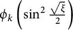 $\phi _k\left (\sin ^2\frac {\sqrt {\xi }}{2}\right )$
(see [Reference Balkanova and Frolenkov4, Theorem 5.14]). This shows that the leading term in the asymptotic expansion of
 $\widehat {W}_{1,1}^{0}(ir)$
is given by
 $$ \begin{align} &\frac{-\pi 4^{ir}\Gamma^2(1/2+ir)}{\Gamma(1+2ir)}\int_{0}^{\pi^2} \eta\left(\tan^2\frac{\sqrt{\xi}}{2}\right) \frac{\cos^{1/2}\frac{\sqrt{\xi}}{2}}{\xi^{1/4}\sin^{1/2}\sqrt{\xi}}Y_0(u\sqrt{\xi}) \left(\frac{\sin\frac{\sqrt{\xi}}{2}}{1+\cos\frac{\sqrt{\xi}}{2}}\right)^{2ir}d\xi \nonumber\\ &\quad = \frac{c_0(r)}{\sqrt{r}}\int_{0}^{\pi/2}\eta\left(\tan^2x\right)Y_0(2ux)(\tan\frac{x}{2})^{2ir}\frac{x^{1/2}dx}{\sqrt{\sin x}}. \end{align} $$
We remark that while further transforming the integral on the right-hand side of (A.44), some constants will occur. For the sake of simplicity, we absorb all these constants in
 $c_0(r)$
without changing the notation.
Now, we can split smoothly the last integral into two parts: first one over
 $ux<u^{\epsilon }$
and the second one over
 $ux>u^{\epsilon }$
. To this end, we use the relation
 $$ \begin{align} \eta(u^{1-\epsilon}x)+\eta(u^{-1+\epsilon}x^{-1})=1. \end{align} $$
Consider the first integral. Note that in this case
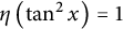 $\eta \left (\tan ^2x\right )=1$
. Let
 $D(f(x))=\frac {\partial }{\partial x}\left (f(x)\sin x\right )$
. Integrating by parts, one has
 $$ \begin{align} &\frac{c_0(r)}{\sqrt{r}}\int_{0}^{\pi/2}\eta (u^{1-\epsilon}x)Y_0(2ux)(\tan\frac{x}{2})^{2ir}\frac{x^{1/2}dx}{\sqrt{\sin x}} \nonumber\\ &\quad =\frac{c_0(r)}{r^{1/2+n}}\int_{0}^{\pi/2}D^n\left(\eta(u^{1-\epsilon}x)\frac{x^{1/2}Y_0(2ux)}{\sqrt{\sin x}}\right) (\tan\frac{x}{2})^{2ir}dx\ll\frac{k^{\epsilon}}{kr^{1/2+n}}. \end{align} $$
Consider the second integral. In this case, the argument of the Bessel function is sufficiently large so that we can write its asymptotic expansion. Once again we can consider only the contribution of the main term given by
 $$ \begin{align} \frac{c_0(r)}{\sqrt{ru}}\sum_{\pm}\int_{0}^{\pi/2}\eta\left(\tan^2x\right)\eta\left(\frac{u^{\epsilon}}{ux}\right)e^{iw_{\pm}(x)}\frac{dx}{\sqrt{\sin x}}, \end{align} $$
 $$ \begin{align} w_{\pm}(x)=\pm2ux+2r\log\left(\tan\frac{x}{2}\right). \end{align} $$
Note that there is no saddle point in the plus case, and therefore, the derivative
 $w^{\prime }_{+}(x)$
is sufficiently large. Integrating by parts, we show that this integral is negligible:
 $$ \begin{align} & \frac{c_0(r)}{\sqrt{ru}}\int_{0}^{\pi/2}\eta\left(\tan^2x\right)\eta \left(\frac{u^{\epsilon}}{ux}\right)e^{iw_{+}(x)}\frac{dx}{\sqrt{\sin x}} \nonumber\\ & \quad\ll \frac{1}{\sqrt{ru}}\int_{0}^{\pi/2}D^n\left(\eta\left(\frac{u^{\epsilon}}{ux}\right)\frac{\eta\left(\tan^2x\right)}{\sqrt{\sin x}}\right)dx\ll \frac{1}{r^{1/2+n}\sqrt{u}}, \end{align} $$
where
 $D(f(x))=\frac {\partial }{\partial x}\left (f(x)\frac {\sin x}{r+u\sin x}\right ).$
Since
 $w^{\prime }_{-}(x)=-2u+\frac {2r}{\sin x}$
, this function has the saddle point
 $\xi _0$
, which is defined as
 $\sin \xi _0=\frac {r}{u}.$
This point belongs to the interval of integration only if
 $$ \begin{align} \eta\left(\tan^2\xi_0\right)\eta\left(\frac{u^{\epsilon}}{u\xi_0}\right)=\eta\left(\frac{r^2}{u^2-r^2}\right)\neq0. \end{align} $$
Note that
 $\eta \left (\frac {u^{\epsilon }}{u\xi _0}\right )=1$
because of the restriction
 $r\gg k^{\epsilon }$
. Therefore, if
 $r>\frac {u(1+\delta )}{\sqrt {1+x_0}}$
(see (6.9)), the saddle point is located outside the interval of integration, and
 $$ \begin{align*}w^{\prime}_{-}(x)=\frac{2r-2u\sin x}{\sin x}\gg\frac{u}{\sin x}.\end{align*} $$
As a result, integration by parts yields the estimate
 $O(r^{-1/2}u^{-1/2-n})$
(similarly to (A.49)). This completes the proof of (A.34).
We are left to investigate the case
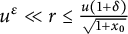 $u^{\epsilon }\ll r\le \frac {u(1+\delta )}{\sqrt {1+x_0}}$
. First, we introduce a smooth partition of unity in the integral (A.47) for the purpose of localizing a saddle point. Accordingly, let
 $\beta (y)$
be a smooth characteristic function of some interval
 $(b_1,b_2)$
such that
 $b_1<1<b_2$
and
 $$ \begin{align} \beta\left(\frac{u\sin x}{r}\right)\eta\left(\tan^2x\right)\eta\left(\frac{u^{\epsilon}}{ux}\right)\neq0 \end{align} $$
for
 $c_1<x<c_2$
with
 $c_2-c_1\gg r/u.$
In the remaining integral with
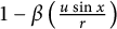 $1-\beta \left (\frac {u\sin x}{r}\right )$
, we have a good lower bound on
 $w^{\prime }_{-}(x)=\frac {2r-2u\sin x}{\sin x}\gg \frac {r}{\sin x}$
, and thus integration by parts works and yields the estimate
 $O(r^{-1/2-n}u^{-1/2})$
. It is left to study the integral:
 $$ \begin{align} I=\frac{c_0(r)}{r}\int_{0}^{\pi/2}\eta\left(\tan^2x\right)\eta\left(\frac{u^{\epsilon}}{ux}\right)\beta\left(\frac{u\sin x}{r}\right)e^{iw_{-}(x)} \sqrt{\frac{r}{u\sin x}}dx. \end{align} $$
Since
 $\beta (u\sin (x)/r)$
localizes x approximately near the point
 $r/u$
, and
 $r\gg k^{\epsilon }$
, it is possible to replace
 $\eta \left (\frac {u^{\epsilon }}{ux}\right )$
by 1. To obtain an asymptotic expansion of the integral (A.52), we apply Lemma 2.2 with
 $$ \begin{align} \Omega_f=\Omega_g=\kappa\asymp\frac{r}{u},\quad \Theta_f\asymp r. \end{align} $$
Consequently, we show that
 $$ \begin{align} I=\frac{c_0(r)}{r\sqrt{|w^{\prime\prime}_{-}(\xi_0)|}} \eta\left(\tan^2\xi_0\right)e^{iw_{-}(\xi_0)}+O\left(\frac{1}{ur^{3/2}}\right). \end{align} $$
Note that when r is close to
 $\frac {u}{\sqrt {1+x_0}}$
, the saddle point
 $\xi _0$
is close to the point where
 $\eta (\tan ^2x)$
becomes 0. To overcome this difficulty, one can simply use the relation
 $\eta (\tan ^2x)=1-\eta (\cot ^2x)$
and evaluate asymptotically two integrals. Combining the results, we again obtain (A.54).
Using
 $$ \begin{align} w_{-}(\xi_0)=-2u\arcsin\frac{r}{u}+2r\log\frac{r}{u+\sqrt{u^2-r^2}},\quad |w^{\prime\prime}_{-}(\xi_0)|=\frac{2u}{r}\sqrt{u^2-r^2} \end{align} $$
Lemma A.4 Let
 $u=k-1/2$
. Then, the following asymptotic formulas hold:
 $$ \begin{align} T_{d}^{1}= \sum_{t_j} \omega_jL^4_j\left(\frac{1}{2}\right)\mathbf{W}_{1,1}(t_j,u) +O\left(\frac{1}{u^{1/2-\epsilon}}\right), \end{align} $$
 $$ \begin{align} T_{c}^{1}= \frac{1}{\pi}\int_{-\infty}^{\infty} \frac{|\zeta\left(\frac{1}{2}+it\right)|^8}{|\zeta(1+2it)|^2}\mathbf{W}_{1,1}(t,u)dt+O\left(\frac{1}{u^{1/2-\epsilon}}\right), \end{align} $$
where
 $$ \begin{align} \mathbf{W}_{1,1}(r,u)=\frac{c_0(r)e^{iw(r,u)}+c_0(-r)e^{-iw(r,u)}}{\sqrt{ur}(u^2-r^2)^{1/4}}\eta\left(\frac{r^2}{u^2-r^2}\right), \end{align} $$
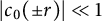 $|c_0(\pm r)|\ll 1$
and
 $w(r,u)$
is given by (A.36).
Proof It follows from (7.1), (5.12), and Lemma A.3 that
 $$ \begin{align} T_{d}^{1}= \frac{(-1)^k}{4}\sum_{t_j\ll k} \omega_jL^4_j\left(\frac{1}{2}\right) \varepsilon_j\left(\widehat{W}_{1,1}^{0}(t_j)+\widehat{W}_{1,1}^{0}(-t_j)\right)+O(k^{-1/2}). \end{align} $$
Note that
 $L_j(1/2)=0$
if
 $\varepsilon _j=-1$
, and therefore, we can omit
 $\varepsilon _j$
in (A.59). Now, (A.56) is a consequence of Lemma A.3 and (A.29).
Using (7.3), (7.4), (5.8), (5.12), and Lemma A.3, we obtain
 $$ \begin{align} T_{c}^{1}= \frac{(-1)^k}{4\pi} \int_{-\infty}^{\infty} \frac{|\zeta\left(\frac{1}{2}+it\right)|^8}{|\zeta(1+2it)|^2} \left(\widehat{W}_{1,1}^{0}(it)+\widehat{W}_{1,1}^{0}(-it)\right)dt+O\left(\frac{1}{u^{1/2-\epsilon}}\right). \end{align} $$
The next result is derived using (1.6), (A.2), (A.17), and Lemma A.4. Notethat
 $L_f(1/2)=0$
if k is odd. Therefore, we can assume that
 $k\equiv 0\pmod {2}$
.
Theorem A.5 For
 $k\equiv 0\pmod {2},$
one has
 $$ \begin{align} \sum_{f\in H_{2k}} \omega_fL^4_f(1/2)=P_6(\log k)+2T_{d}^{1}+2T_{c}^{1}+O(k^{-1+\epsilon}), \end{align} $$
where
 $T_{d}^{1}$
and
 $T_{c}^{1}$
are given by (A.56) and (A.57), respectively.
Remark Note that
 $\mathbf {W}_{1,1}(r,u)=0$
if
 $|r|\gg k.$
Thus, we are summing in (A.56) over
 $|t_j|\ll k$
, and the integral in (A.57) is taken over
 $|t|\ll k$
. Using (A.29) and (A.30), we prove the following trivial estimates:
 $$ \begin{align} T_{d}^{1}\ll k^{1/2+\epsilon}, \quad T_{c}^{1}\ll k^{\epsilon}. \end{align} $$
Proof of Theorem 1.2
To prove (1.8), we consider the average of (A.61). In order to estimate
 $$ \begin{align} \sum_{\substack{L<k\le 2L\\k\equiv 0\pmod{2} }}T_{d}^{1}+T_{c}^{1}, \end{align} $$
we just need to obtain an upper bound for the average of
 $\mathbf {W}_{1,1}(r,u)$
over
 $k.$
Using (A.36), we show that
 $$ \begin{align} \frac{\partial}{\partial u}w(r,u)=-2\arcsin\frac{r}{u}. \end{align} $$
Therefore,
 $$ \begin{align*}|\frac{\partial}{\partial k}w(r,2k-1/2)|<2\pi-\delta_0.\end{align*} $$
Using the generalization of [Reference Titchmarsh27, Lemma 4.10] given in [Reference Karatsuba19, Lemma 1, Section 3], we have
 $$ \begin{align} \sum_{\substack{L/2<k\le L}}\mathbf{W}_{1,1}(r,2k-1/2)=\int_{L/2}^{L}\mathbf{W}_{1,1}(r,2x-1/2)dx+O\left(\frac{L^{\epsilon}}{L\sqrt{r}}\right). \end{align} $$
To estimate the integral, we apply the first derivative test [Reference Titchmarsh27, Lemma 4.3], proving that
 $$ \begin{align} \sum_{\substack{L/2<k\le L}}\mathbf{W}_{1,1}(r,2k-1/2)\ll\frac{1}{r^{3/2}}+\frac{L^{\epsilon}}{L\sqrt{r}}. \end{align} $$
Finally, using (A.66), (A.29), and (A.30), we infer
 $$ \begin{align} \sum_{\substack{L<k\le 2L\\k\equiv 0\pmod{2} }} T_{d}^{1}+ T_{c}^{1}\ll L^{1/2+\epsilon}.\\[-34pt]\nonumber \end{align} $$
Proof of Theorem 1.3
It is required to estimate the average of
 $T_{d}^{1}+T_{c}^{1}$
. To this end, it is enough to evaluate the average of
 $\mathbf {W}_{1,1}(r,u)$
, namely,
 $$ \begin{align} \sum_{k}\exp\left(-\left(\frac{k-K}{G}\right)^2\right)\mathbf{W}_{1,1}(r,2k-1/2). \end{align} $$
To do this, we argue in the same way as in [Reference Balkanova and Frolenkov4, Lemma 7.3], starting with an application of the Poisson summation formula:
 $$ \begin{align} \sum_{k}\exp\left(-\left(\frac{k-K}{G}\right)^2\right)\mathbf{W}_{1,1}(r,2k-1/2)=\sum_{m \in \mathbf{Z}}P(m),\quad \end{align} $$
 $$ \begin{align} P(m)=\int_{-\infty}^{\infty}\exp\left(-\left(\frac{y-K}{G}\right)^2\right)\mathbf{W}_{1,1}(r,2y-1/2)e(-my)dy. \end{align} $$
Making the change of variable
 $y=K+Gx$
and using (A.58), one has
 $$ \begin{align} P(m)\ll\frac{G}{\sqrt{r}}\int_{-\infty}^{\infty}\exp\left(-x^2\right)\eta\left(\frac{r^2}{4(K+Gx)^2-r^2}\right) \frac{e^{ig(r,K,m,x)}dx}{\sqrt{K+Gx}(4(K+Gx)^2-r^2)^{1/4}}, \end{align} $$
where
 $g(r,K,G,m,x)=w(r,2K+2Gx-1/2)-2\pi mGx.$
It follows from (A.64) that for
 $m\neq 0,$
 $$ \begin{align} \frac{\partial}{\partial x}g(r,K,G,m,x)=-4G\arcsin\frac{r}{2(K+Gx)-1/2}-2\pi mG\gg mG. \end{align} $$
Therefore, multiple integration by parts leads to the bound
 $P(m)\ll (mG)^{-A}.$
In the case
 $m=0$
, one has
 $$ \begin{align} \frac{\partial}{\partial x}g(r,K,G,0,x)=-4G\arcsin\frac{r}{2(K+Gx)-1/2}\gg \frac{Gr}{K}, \end{align} $$
and multiple integration by parts yields
 $P(0)\ll (Gr/K)^{-A}.$
Hence, for
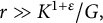 $r\gg K^{1+\epsilon }/G,$
one has
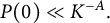 $P(0)\ll K^{-A}.$
In the case when
 $r\ll K^{1+\epsilon }/G$
, we have the trivial bound
 $P(0)\ll G/\sqrt {rK^2}$
. Using (A.56) and applying the estimates proved above, we show that
 $$ \begin{align} \sum_{k}\exp\left(-\left(\frac{k-K}{G}\right)^2\right)T_{d}^{1}\ll \frac{G}{K}\sum_{t_j\ll K^{1+\epsilon}/G}\frac{\omega_j}{\sqrt{t_j}}L^4_j\left(\frac{1}{2}\right)+\frac{G^{1+\epsilon}}{K^{1/2}}\ll \frac{K^{1/2+\epsilon}}{G^{1/2}}+\frac{G^{1+\epsilon}}{K^{1/2}}. \end{align} $$
Arguing in the same way with the use of (A.30), we conclude that
 $$ \begin{align} \sum_{k}\exp\left(-\left(\frac{k-K}{G}\right)^2\right)T_{c}^{1}\ll K^{\epsilon}+\frac{G^{1+\epsilon}}{K^{1/2}}. \end{align} $$
Finally, we remark that the estimates (A.74) and (A.75) are better than the averaged main term if
 $G\gg K^{1/3+\epsilon }$
. This completes the proof of (1.9).
Acknowledgements
We thank the referee for carefully reading our manuscript and providing helpful comments.



