

Introduction
Close range hyperspectral imagery is a promising tool for phenotyping or crop monitoring. In association with Partial Least Square Regression or PLS-R (Wold et al., Reference Wold, Sjöström and Eriksson2001), it allows to build high spatial resolution maps of chemical content at the canopy level.
However, several optical phenomena must be taken into account when applying this approach to vegetation scenes in natural conditions. Among them, specular reflection and multiplicative factors due to leaf inclination can be overcome by pre-processing (Vigneau et al., Reference Vigneau, Ecarnot, Rabatel and Roumet2011). But the most challenging phenomenon is multiple scattering: when a leaf receives part of its lighting from surrounding leaves, the incident light spectrum and thus the apparent reflectance are modified, leading to false regression results. Moreover, for practical reasons, it is impossible to include multiple scattering examples in a PLS-R calibration set.
We propose here an original method based on the analytic formulation of scattering, to be used in association with PLS-R. It only requires isolated leaf samples in its learning step. It has been developed using canopy and light propagation simulation tools, and evaluated on real crop plants for leaf nitrogen content assessment.
Theory of operation
Oblique projection for classification
Let us consider a regression problem based on spectral data, where every incoming spectrum (issued from some measurement) has to be processed to estimate the value of a variable of interest. Usually, the solution to this problem requires a learning data set, which consists in couples of spectra and associated output values. A main issue of this approach is when the shape of the measured spectra is influenced by an undesirable external factor (e.g. temperature), because various examples of this influence must be represented in the learning set, in order to preserve the efficiency of the model. A general solution was proposed by Roger et al. (Reference Roger, Chauchard and Bellon Maurel2003) in the frame of PLS-R: as soon as the main axes of influence of this external factor in the spectral space have been determined, they can be used to compute an orthogonal projection of every spectrum before PLS-R processing.
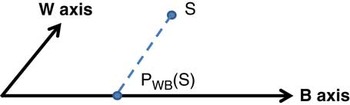
However, this orthogonal projection can lead to information loss when the projection axes are close to the direction of influence of the variable of interest. Let us call B the subspace generated by the variable of interest in the spectral space and W the subspace generated by the external factor. If we are able to determine these both subspaces, a possible solution is to consider an oblique projection on the subspace B (Figure 1). When B and W are multidimensional subspaces with a non-empty intersection, this intersection must be removed from the W subspace before projection, in order to avoid information loss.
Oblique projection of a spectrum S

Application to multiple scattering removing in hyperspectral data
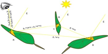
Let us consider a leaf with a reflectance spectrum that is observed in its natural environment from a camera above the canopy. As described in (Vigneau et al., Reference Vigneau, Ecarnot, Rabatel and Roumet2011), its apparent reflectance can be affected by multiplicative and additive terms due to leaf inclination and specular reflection. Moreover, because the leaf is partially illuminated by light reflected by neighboring leaves, nonlinear additive terms are also added. This phenomenon is known as multiple scattering. Figure 2 illustrates the case of a leaf surrounded by others leaves with similar reflectance and transmittance properties, respectively referred as R and T. It shows that additive term R2, TR2, TR3, etc. can be added to the observed reflectance R, with scalar factors related to leaf inclination.
Some cases of leaf illumination in its natural environment. E: lighting source radiance. R: leaf reflectance. L: observed radiance. β1, β2, β3 are scalar factors related to leaf inclination

In applications where the observed reflectance is used to assess biological traits by comparing its values in various bands, this can lead to strong overestimations. As an example, it is well known that chlorophyll and nitrogen content of leaves is highly related to the ratio of their reflectance amplitudes in the near-infrared and red bands. Considering a reflectance spectrum R2 instead of R will increase this ratio, leading to overestimation.
Formally, according to the notations above, it means that multiple scattering induces a spectral deviation subspace W that is not orthogonal to the deviation subspace B. Therefore, in order to overcome its effects, we propose to apply an oblique projection transformation to every observed spectrum. For this purpose, we have to determine W and B.
Let us consider a learning set made of n triplets (Ri, Ti, yi), where Ri,Ti are the reflectance and transmittance spectra of a leaf i and yi is the value of given chemical trait (e.g. nitrogen content) for this leaf. We can thus compute the subspace W by gathering all the additive terms generated by multiple scattering, using the following procedure:
-
- For every spectrum Ri, polynomial terms RiuTiv are computed and normalized as unitary vectors. The covariance matrix of all these vectors is then computed, and the first eigenvectors are retained.
-
- All retained eigenvectors for all leaves i are then concatenated as the column vectors of a matrix MW, and the total inertia matrix is computed as: W=MW.MWT.
To compute the subspace B, let us consider temporarily that the n values yi of the learning set are distributed among N classes. B can thus be approximated as the interclass inertia of the reflectance spectra Ri for these N classes, i.e. as the inertia of the N class centers.
As a summary, three tunable parameters must be managed for the computation of the projection matrix: the maximum degree maxD of the polynomial terms, the maximum number maxP of eigenvectors that are retained for each spectrum Ri, and the maximum number maxW of eigenvectors that are retained for the final subspace W.
Material and methods
Method development by simulation
A total of 57 reflectance and transmittance spectra of wheat leaves (elite variety) have been used for the simulations. There were acquired during the season 2014 in field microplots (Montpellier experimental station, INRA, South France), cultivated under various nitrogen amendment conditions. Spectra were collected on full expanded leaves using a field spectrometer equipped with a leaf clip (FieldSpec®, Analytical Spectral Devices, Inc. (ASD), Boulder, Colorado, USA). In addition, a chemical reference of leaf nitrogen content (LNC) expressed as a percentage of dry matter mass was measured in laboratory for each collected leaf using a chemical analyzer (Ecarnot et al ( Reference Ecarnot, Compan and Roumet2013 )).
The ASD spectra (initially 350-2500 nm range with 1 nm step) were reduced and resampled to the 400-1100 nm range with 5 nm steps. As a result, a data set of 57 triplets (Rj(λ), Tj(λ), LNCj) was available for this study, with 141 λ values and a LNC range from 0.55 to 4.53% of dry matter (DM). Rj spectra are referred as “basic” spectra in the following.
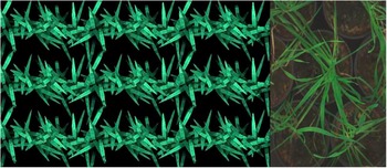
A wheat canopy model has then been built using simulation models included in the open source software platform Open-Alea (http://openalea.gforge.inria.fr/dokuwiki/doku.php. Last access December 2016): Adel-Wheat, a 3D dynamic model of the aerial growth of winter wheat (Fournier et al Reference Fournier, Andrieu, Ljutovac and Saint-Jean2003), has been associated with the Caribu light propagation model (Chelle & Andrieu, Reference Chelle and Andrieu1998), using the reflectance and transmittance data mentioned above, in order to synthetize realistic hyperspectral images. For each given basic spectrum, an image containing more than one thousand simulated spectra in multiple scattering conditions has been simulated (Figure 3. left).
Examples of hyperspectral images in false colors (670 nm, 600 nm, 450 nm bands have been used as R, G, B channels) Left: synthetic image built with Caribu. Right: Plant image

PLS-R models have then been built using the set of couples (Rj(λ), LNCj) as learning set, and applied to the apparent reflectance spectra issued from the synthetized images. Two kinds of PLS-R models have been considered: the first one using directly the Rj(λ) reflectance spectra after a SNV (standard normal variate) preprocessing, the second after applying an oblique projection before the SNV, both for the learning and the test set.
The oblique projection matrix was built by partitioning the couples (Rj(λ), LNCj) in 10 different classes according to the LNCj values, in order to compute the inter-class inertia matrix B. For the determination of W, various combinations of parameters maxD, maxP and maxW were tested, and the combination giving the best results has been retained.
Method assessment in real conditions
200 seeds of durum wheat (anvergur) have been seeded in pots of diameter 20 cm and grown in green house conditions for 8 weeks, with various nitrogen amendment levels. Ten pots have been imaged from nadir using a hyperspectral camera Hyspex VNIR-1024 (Norsk Elektro Optikk, Skedsmokorset, Norway). For this purpose, the pots were surrounded with 8 other ones, in order to reproduce as much as possible multiple scattering conditions, and a Spectralon® with a flat reflectance value of 0.5 was included in each scene for lighting reference and reflectance correction (Figure 3. right).
Three individual leaves were then located in each pot and removed. There were laid on a black sheet of paper to be imaged with no multiple scattering. Finally, their local nitrogen content was measured in 4 different points along the leaf, using an ASD field spectrometer coupled with the PLS-R model developed in (Ecarnot et al., Reference Ecarnot, Compan and Roumet2013), leading to a total set of 10×3×4=120 nitrogen values.
All hyperspectral images were then transformed in reflectance images according to the Spectralon® reference. Spectra in the leaf zones corresponding to ASD measurement were then collected in the images of flat isolated leaves, and used as basic spectra to build PLS-R models with and without oblique projection. For the oblique projection, parameters maxD, maxP and maxW chosen by simulation were used again. The PLS-R models were then applied to plant images.
Results and discussion
Simulation results
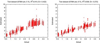
PLS-R models were calibrated on the set of basic spectra and applied to the simulated spectra issued from Caribu. The following parameters have been retained for the projection matrix: maxD=14, maxP=2; maxW=5. As shown in Figure 4, the standard error is substantially reduced by this projection (0.272% DM instead of 0.422% DM).
LNC prediction plots on simulated spectra (%DM). Left: standard PLS-R model. Right: PLS-R model after oblique projection

Tests on real plants
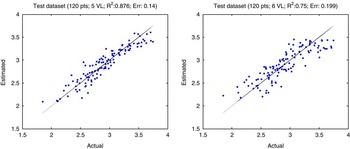
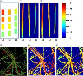
According to ASD measurements, a LNC range from about 2 to 3.5% of dry matter (DM) was obtained from isolated leaves, and it was observed that all leaves have an increasing LNC from the base to the end. Two PLS-R models were built without and with oblique projection, with a cross-validation error below 0.2% DM for both of them.
As shown in Figure 5, the oblique projection slightly degrades the prediction quality. Indeed, the projection induces a slight loss of spectral information, due to the approximate determination of the B subspace. However, Figure 6 shows that both models give nearly the same results on isolated leaves, but very different ones on plant images: PLS-R with no projection seems to generate an over prediction of LNC.
LNC learning prediction plots of PLS-R models (%DM) (left: with no projection; right: with projection)

LNC prediction results (%DM) on hyperspectral images at the leaf level. a: ASD measurement positions and values. b, c: prediction on isolated leaves without (b) and with (c) oblique projection. d, e, f: prediction on the same leaves before cutting (natural image (d), image processed without (e) and with (f) oblique projection

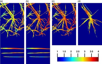
Figure 7a and Figure 7b confirm that both PLS-R models give the same predictions on isolated leaves and different ones on standing leaves. Moreover, Figure 7c and Figure 7d clearly show the influence of surrounding plants on the LNC prediction results obtained with a standard PLS-R model, due to various levels of multiple scattering.
LNC prediction (%DM) in various surrounding conditions. a,b: Isolated and standing leaves in the same image, models with (a) and without (b) projection. c,d: surrounded and isolated pot , model without projection.

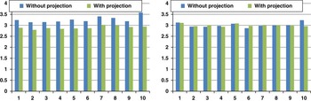
In order to confirm these observations on a larger set of data, the ten images combining both pot plants and isolated leaves have been processed with both PLS-R models, and the LNC values have been averaged separately for the two kinds of leaves (Figure 8). Once again, a systematic overestimation is obtained with the PLS-R model without projection for standing leaves, while mean values remain nearly similar for both models on isolated leaves.
Average predicted LNC values (%DM) for ten pot plant images. All images include standing (left) and isolated (right) leaves areas.

Conclusion
A new method has been proposed to overcome the impact of multiple scattering in the processing of hyperspectral images of crop plants by PLS-R. This method is based on the physical interpretation and formalization of scattering phenomenon, and its detailed parameters have been determined using simulation tools. Though a more accurate evaluation is still necessary, very promising results have been obtained on real durum wheat plants, and the considerable impact of plant environment on the prediction of standard PLS-R has been confirmed as well.
Acknowledgements
This study has been supported by Agropolis Foundation under the reference ID 1202-008 through the ‘Investissements d’avenir’ program (Labex Agro:ANR-10-LABX-0001-01).