


INTRODUCTION
In the basic model of representative democracy, voters elect legislative representatives whose positions reflect the preferences of their respective districts’ median voters. These representatives convene in an amorphous assembly—one in which parties do not play an important role—and national policy is set to correspond to the preferences of the median representative in this assembly. Thus, the legislature is composed of representatives who are more moderate than the voters who elect them, and actual policy and legislation reflects the most moderate position in this assembly of moderates (a prediction that appears somewhat incorrect).
There is, of course, a large body of literature modeling interactions of representatives in a legislature and the effects of legislative institutions such as the power of specialized committees, but this literature takes the set of legislators as given. There is also a large literature on political competition, but that literature generally assumes that candidates either unilaterally choose or are exogenously endowed with policy positions that enter voters’ utility functions directly and exclusively. That is, voters care only about the positions of those candidates that they personally can decide between. In this paper, we build a model of electoral competition that combines these two strands of literature: When voting for their local representative, the voters in our model explicitly take into account that they are not in a position to determine the unilaterally decisive policy maker in the nation, but rather just one of many representatives who interacts with other representatives in the determination of policy.
Our model is based on two realistic ingredients: First, the majority party in a legislature is an important power center influencing the crafting of policy, and so voters naturally care not only about the positions espoused by their local candidates, but also about the national positions of the parties with whom these local candidates are affiliated. A potential microfoundation for why voters care about national party positions is that no legislator is a specialist in all policy areas, and therefore they all have to rely sometimes on the expertise of their fellow party members (Shepsle and Weingast Reference Shepsle and Weingast1987; Gilligan and Krehbiel Reference Gilligan and Krehbiel1989). The importance of the majority party for law-making creates important spillover effects between the candidates of the same party who run in different districts. Second, legislative candidates are nominated by policy-motivated primary voters who, like the general election median voter, care about both national party and local candidate positions, but have more extreme ideal positions. A central question in our analysis is how national party positions affect the competitive pressure to nominate moderate candidates, which plays a central role both in the classical Downsian model, and in the policy-motivated candidates model.
While parties play a crucial role in the legislature for shaping politics and policy, there is surprisingly little analysis of how the fact that each candidate is connected to a party and thus, implicitly, to the positions of candidates of that party from other districts influences nomination decisions, as well as election outcomes in different legislative districts.
Applying the simplest Downsian model naively to Congressional elections—which much of the empirical literature implicitly does—generates empirically incorrect predictions: Since, in the Downsian model, all candidates adopt the preferred position of their district’s median voter, all voters should be policywise indifferent between the Democratic candidate and his Republican opponent. Thus, Republicans in New England or Democrats in rural Western districts should have a substantial chance to be elected to Congress if only they match their opponent’s policy platform.Footnote 1 Furthermore, in this framework, gerrymandering districts affects only candidate positions in the gerrymandered districts but does not help a party to increase their expected representation in Congress. These predictions are certainly empirically incorrect, but understanding why is challenging.
In our model, voters’ utility depends on both their local representative’s position, and the position of the majority party. In the general election, voters take into account the two local candidates’ positions, as well as the chance that the election outcome in their district may change which party is the majority party in the legislature.
The latter effect implies that, in most districts, the median voter cares not just about the local candidates’ positions when deciding whom to vote for, but also about their party labels, as they are associated with different national positions. The favored party’s primary voter can exploit this situation by nominating a more extreme candidate than the general election median voter would prefer. In particular, if voters care sufficiently strongly about national positions relative to local candidate positions, then the favored party’s primary voter can simply nominate his own preferred candidate and still win, generally even with a strict supermajority of votes.
The local general election loses some of its disciplining force because the voters’ national preference factors in their vote choice. The electoral prospects of candidates in a given district are influenced by the expected ideological position of their parties’ winning candidates elsewhere. The association with a party that is not attuned with a district’s ideological leanings may be poisonous for a candidate, even if his own policy positions are tailor-made for his district.
Consider, for example, Lincoln Chafee, the former Republican U.S. senator from Rhode Island, who had taken a number of moderate and liberal positions that brought him in line with voters in his state.Footnote 2 As the New York Times reported, in the 2006 election, “exit polls gave Senator Lincoln Chafee a 62 percent approval rating. But before they exited the polls, most voters rejected him, many feeling it was more important to give the Democrats a chance at controlling the Senate.”Footnote 3 His Democratic challenger Whitehouse “succeeded by attacking the instances in which Chafee supported his party’s conservative congressional leadership (whose personalities and policies were very unpopular, state-wide).”Footnote 4
In a review of 2006 campaign ads, factcheck.org summarized: “President Bush was far and away the most frequent supporting actor in Democratic ads [. . .] The strategy is clear: whether they’re referring to a Republican candidate as a ‘supporter’ of the ‘Bush agenda’ or as a ‘rubberstamp,’ Democrats believe the President’s low approval ratings are a stone they can use to sink their opponents [. . .] Democratic Sen. Hillary Clinton of New York got the most mentions in Republican ads holding forth the supposed horrors of a Democratic-controlled Senate [. . .] The runner-up is ‘San Francisco Liberal Nancy Pelosi,’ who is mentioned in at least 6 GOP ads as a reason not to vote for a Democrat who would in turn vote to make her Speaker of the House.”Footnote 5
In contrast to the classical one-district spatial model, the ideological composition of districts in our model does not only influence the ideological position of elected candidates, but also the chances of parties to win, thus increasing partisan incentives for gerrymandering. Gerrymandering or, more generally, the intensification of the median ideological preferences in some districts, affects the political equilibrium even in those districts where the median voter preferences remain the same as before. Our results imply that testing for the causal effect of gerrymandering on polarization in Congress is more complicated than the existing literature has recognized.
RELATED LITERATURE
Ever since Downs’s (Reference Downs1957) seminal work, candidates’ position choice is a central topic in political economy. While the classical median voter framework identifies reasons for platform convergence, many subsequent electoral competition models develop different reasons for policy divergence, including policy motivation (Wittman Reference Wittman1983; Calvert Reference Calvert1985; Londregan and Romer Reference Londregan, Romer, Barnett, Hinich and Schofield1993; Osborne and Slivinski Reference Osborne and Slivinski1996; Besley and Coate Reference Besley and Coate1997; Martinelli Reference Martinelli2001; Gul and Pesendorfer Reference Gul and Pesendorfer2009); entry deterrence (Palfrey Reference Palfrey1984; Callander Reference Callander2005); agency problems (Van Weelden Reference Van Weelden2013); incomplete information among voters or candidates (Castanheira Reference Castanheira2003; Bernhardt, Duggan, and Squintani Reference Bernhardt, Duggan and Squintani2007; Callander Reference Callander2008); and differential candidate valence (Bernhardt and Ingberman Reference Bernhardt and Ingberman1985; Groseclose Reference Groseclose2001; Krasa and Polborn Reference Krasa and Polborn2010b, Reference Krasa and Polborn2012; Bierbrauer and Boyer Reference Bierbrauer and Boyer2013).
Most of the literature looks at isolated one-district elections. Exceptions are Austen-Smith (Reference Austen-Smith1984); Snyder (Reference Snyder1994); Ansolabehere, Leblanc, and Snyder (Reference Ansolabehere, Leblanc and Snyder2012) and subsequent work by Polborn and Snyder (Reference Polborn and Snyder2017). In Austen-Smith (Reference Austen-Smith1984), the party that wins the majority of n districts implements an aggregate of its candidates’ positions. Each district candidate chooses his position to maximize his chance of winning. If an equilibrium exists, then both party positions fully converge to the median voter in the median district, even though individual candidates’ positions differ. In contrast, in our model, positions are chosen by policy-motivated primary voters, and voters care about both national party positions and local candidates. In our equilibrium, national party positions diverge, and we can analyze the effects of gerrymandering and of more or less radical primary voters.
Snyder (Reference Snyder1994) considers a dynamic setting in which voters care only about national party positions that are chosen by the party’s representatives in the pre-election legislature to maximize their individual reelection chances. In Ansolabehere, Leblanc, and Snyder (Reference Ansolabehere, Leblanc and Snyder2012), a special version of this model, the left and the right party locate at the 25th and 75th percentile of the district median distribution. Polborn and Snyder (Reference Polborn and Snyder2017) analyze a model of legislative competition in which only the two parties’ national positions matter for voters and are determined by the median caucus member. Their main focus is on deriving comparative static predictions about the effects of idiosyncratic (i.e., candidate-specific) valence uncertainty and systematic electoral shifts (as in wave elections, where one party does better in most districts than in previous elections) on polarization, and testing them empirically. To focus on these comparative static predictions, their model of candidate competition is much simpler than ours, essentially assuming that the local candidates perfectly represent the median voter in their respective districts. In contrast, our focus is on the effect of the nomination process in which candidates are chosen by policy-motivated primary voters, who, as we show, generally select nominees who are more extreme than the general election median voter of the district would prefer.
In the influential models of Erikson and Romero (Reference Erikson and Romero1990) and Adams and Merrill (Reference Adams and Merrill2003), voters receive, in addition to the payoff from the elected candidate’s position, a “partisan” payoff from his party affiliation, which, however, is exogenous and orthogonal to his policy position. Our model provides a microfoundation for these partisan payoffs, and shows how they depend on the equilibrium polarization between the parties’ candidates in other districts, and how they, in turn, affect the candidates’ equilibrium positions.
Probabilistic voting models (e.g., Lindbeck and Weibull Reference Lindbeck and Weibull1987; Dixit and Londregan Reference Dixit and Londregan1995), as well as differentiated candidates models (DCMs; Aragones and Palfrey Reference Aragones and Palfrey2002; Soubeyran Reference Soubeyran2009; Krasa and Polborn Reference Krasa and Polborn2010a, Reference Krasa and Polborn2010b, Reference Krasa and Polborn2012, Reference Krasa and Polborn2014; Camara Reference Camara2012), often consider an exogenous valence dimension. In the spirit of the DCM, one can interpret party affiliation in our model as a fixed characteristic, but in contrast to existing DCMs, voters’ preferences over characteristics (i.e., the candidates’ party affiliations) depend on national party positions and therefore, ultimately, on positions of candidates in other districts.
Our model assumes that national party positions matter for voters,Footnote 6 and a significant number of models explains why this is so. Conditional party government theory (Rohde Reference Rohde2010; Aldrich Reference Aldrich1995) and endogenous party government theory (Volden and Bergman Reference Volden and Bergman2006; Patty Reference Patty2008) argue that party leaders can use incentives and resources to ensure cohesiveness of their party. Procedural cartel theory (Cox and McCubbins Reference Cox and McCubbins2005) argues that party leadership can at least enforce voting discipline over procedural issues. Castanheira and Crutzen (Reference Castanheira and Crutzen2010), Eguia (Reference Eguia2011a, Reference Eguia2011b) and Diermeier and Vlaicu (Reference Diermeier and Vlaicu2011) provide theories of endogenous institution choice leading to powerful parties. All these models of the importance of parties in Congress take the distribution of legislator preferences as exogenously given, while our model provides for an electoral model and thus endogenizes the types of elected legislators.
MODEL
A polity is divided into a set of districts I, where  $\#I$ is odd. Each district i contains three strategic agents: a local Democratic leader, a local Republican leader, and a general election median voter.
In the first stage, in each district i, the local leader of each party P = D, R chooses the position  $x_{i,P}\in \mathbb {R}$ of party P’s candidate in district i. The local party leaders can be thought of as a shorthand for the decisive voter in the respective party’s primary election that decides which candidate to nominate. We therefore assume that these local party leaders are not interested in winning per se, but rather, like any other voter, derive utility from policy (with details explained below).
In the second stage, there is a general election in all districts. In addition to their local candidates’ positions, each party has a national policy X P that it can implement if it receives a majority in the legislature. The national policy position is not a strategic choice by any particular player, but rather some aggregate of the positions of a party’s legislators, discussed further below.
The utility of a voter with ideal position θ from district i is
 $$\begin{eqnarray}
u_\theta (X_P,x_{i,Q})=-(1-\gamma ) (X_P-\theta )^2-\gamma (x_{i,Q}-\theta )^2, \nonumber\\
\end{eqnarray}$$
where γ ∈ (0, 1) is the voter’s weight on the local representative’s position, the policy of the district’s elected representative is x i, Q, where Q ∈ {D, R} is the representative’s party, and the policy of the majority party P in the legislature is X P.
If voters only care about the policy implemented by the legislature, then the value of γ is zero. There are at least two conceptually distinct reasons why γ might be positive. First, voters may attach an expressive value to their actual vote; that is, a voter may derive utility from voting for a local candidate whose position he likes (or opposing one that he dislikes) even if he recognizes that national policy is determined by national party positions. Second, representatives may have special influence on policy that is particularly relevant for their district, for example, through funding projects in their district whose payoffs depend on ideology. Note that the case where each election is completely independent of what happens in the rest of the country (i.e., where literally “all politics is local” and nobody cares about national legislation) corresponds to γ = 1.Footnote 7
Ex ante, there is uncertainty about the ideal position of district i’s median voter, described by a cdf Φi(·) that is symmetric about μi. Let p i denote the probability that district i is decisive in determining which party has a majority in the legislature (i.e., p i is the probability that both parties win the same number of representatives in all other districts  $j\not=i$). Note that p i can either be derived by the equilibrium played in other districts or can simply be thought of as reflecting the (not necessarily rational) perception of the voters in district i that their district is pivotal.Footnote 8
In summary, the game proceeds as follows:
1. In each district i, the local Democratic leader with ideal point d i selects the Democratic candidate’s position to maximize his expected utility, taking as given the probability that the district is decisive, p i, and the party policies, X D and X R.Footnote 9 Similarly, the local Republican leader with ideal point r i selects x i, R, with an analogous objective.
2. In each district i, the median voter M i is realized, and votes for his preferred candidate, if any. If M i is indifferent between Democrat and Republican, he votes for the candidate of the party whose national position he prefers (if any), or otherwise randomizes.Footnote 10
EQUILIBRIUM
Our analysis starts with stage 2 of the game. The local median voter M i has expected utility piu Mi(XR, x i, R) + (1 − pi)EP[u Mi(XP, x i, R)] if the Republican candidate wins, where E P[·] is the expectation over which party wins a majority, given that district i is not pivotal. Similarly, if the Democrat wins, M i’s expected payoff is piu Mi(XD, x i, D) + (1 − pi)EP[u Mi(XP, x i, D)]. Using the utility function in Equation (1), it follows that median voter M i prefers the Democrat to the Republican if
 $$\begin{eqnarray}
&&-p_i(1-\gamma )(X_D-M_i)^2 - \gamma (x_{D,i}-M_i)^2\ge \nonumber\\
&&\quad -\,p_i(1-\gamma )(X_R-M_i)^2 - \gamma (x_{R,i}-M_i)^2.
\end{eqnarray}$$
Let the indifferent voter type for whom Equation (2) holds as equality be denoted by
 $$\begin{equation}
\theta (x_{i,D},x_{i,R})=\frac{1}{2} \frac{ (1-\gamma )p_i(X_R^2-X_D^2)+\gamma (x_{i,R}^2-x_{i,D}^2)}{ (1-\gamma )p_i(X_R-X_D)+\gamma (x_{i,R}-x_{i,D})}.
\end{equation}$$
Then M i prefers to vote for the Democrat if and only if M i ⩽ θ(x i, D, x i, R). The probability that the Democrat wins in district i is therefore Φi(θ(x i, D, x i, R)).
For example, if the district cannot be pivotal (p i = 0), then Equation (3) implies that θ(·) = (x i, R + x i, D)/2, that is, the median voter chooses the candidate whose platform is closest to M i. The probability that the Democrat wins is therefore 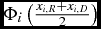 $\Phi _i\left(\frac{x_{i,R}+x_{i,D}}{2}\right)$.
Now consider the first stage of the game. The Democratic leader with ideal point d i chooses x i, D to maximize his expected payoff, that is,
 $$\begin{eqnarray}
\max _{x_{i,D}} &- &\Phi _i(\theta (x_{i,D},x_{i,R}))\Bigl ((1-\gamma )\nonumber\\
&&\times\,p_i(X_D-d_{i})^2+\gamma (x_{i,D}-d_{i})^2\Bigr ) \nonumber\\
&-& \Bigl (1 -\Phi _i(\theta (x_{i,D},x_{i,R}))\Bigr )\Bigl ((1-\gamma )\nonumber\\
&&\times\,p_i(X_R-d_{i})^2+\gamma (x_{i,R}-d_{i})^2\Bigr ) \nonumber \\
&-&(1-p_i)(1-\gamma )E_P\bigl [(X_P-d_{i})^2\bigr].
\end{eqnarray}$$
Similarly, the Republican primary voter solves
 $$\begin{eqnarray}
\max _{x_{i,R}} &-& \Phi _i(\theta (x_{i,D},x_{i,R}))\Bigl ((1-\gamma )\nonumber\\
&&\times\,p_i(X_D-r_{i})^2+\gamma (x_{i,D}-r_{i})^2\Bigr ) \nonumber\\
&-& \Bigl (1 -\Phi _i(\theta (x_{i,D},x_{i,R}))\Bigr )\Bigl ((1-\gamma )\nonumber\\
&&\times\,p_i(X_R-r_{i})^2+\gamma (x_{i,R}-r_{i})^2\Bigr ) \nonumber\\
&-&(1-p_i)(1-\gamma )E_P\bigl [(X_P-r_{i})^2\bigr].
\end{eqnarray}$$
Definition 1 Policies xi, D and xi, R are an equilibrium in district i if and only if xi, D solves Equation (4) and xi, R solves Equation (5).
If p i = 0, then all terms that reflect the parties’ national positions drop out and the optimization problem reduces to that of a standard Calvert-Wittman model. As mentioned above, in this case θ(x i, D, x i, R) = (x i, D + x i, R)/2. Thus, after substituting p i = 0, dropping the third (constant) term in Equation (5), and dividing by γ, the Republican primary voter’s problem is equivalent to
 $$\begin{eqnarray}
&&\max _{x_{i,R}} -\Phi \left(\frac{x_{i,D}+x_{i,R}}{2}\right)(x_{i,D}-r_{i})^2 \nonumber\\
&&\quad- \left(1 -\Phi \left(\frac{x_{i,D}+x_{i,R}}{2}\right)\right)(x_{i,R}-r_{i})^2;
\end{eqnarray}$$
and similar for the Democrat. Formally, this is equivalent to the standard problem of policy motivated candidates with ideal points r i and d i, respectively, who trade off the probability of winning and selecting a policy that is closer to their ideal point.Footnote 11
If, instead, p i > 0, there is no closed form solution for the equilibrium in this case.Footnote 12 To learn something about the structure of equilibrium, we proceed with our analysis by varying the importance of national and local issues for voters, γ. Note that this importance can plausibly vary over time and between different chambers.Footnote 13 In the first of the following subsections, we deal with the case that the uncertainty about the median voter’s position is described by a uniform distribution with sufficiently small range. In the second and third subsection, we analyze the limit cases of γ ≈ 0 (i.e., voters care mostly about national party positions) and γ ≈ 1 (the Calvert-Wittman benchmark); we can do this without imposing any assumptions on the uncertainty about the median voter positions.
Intermediate Weights on Local vs. National Positions
We start with the general case that voters care about both local candidate positions and national party positions in a way that both components have a non-negligible weight in their utility function (i.e., γ takes an intermediate value). Tractability requires us to focus on the case where the distribution of the median voter is uniform on some interval [μi − c, μi + c], with c small.
Given that the uniform distribution has bounded support, in sufficiently extreme districts, the favored party’s advantage is so large that they can win in district i even if they choose a candidate who is located at the respective leader’s ideal point. For example, if θ(d i, x i, R) > μi + c for all possible positions x i, R of the Republican candidate,Footnote 14 then the Democrats can win for sure in district i by nominating a candidate with position x i, D = d i (which, clearly, is optimal in this case). Similarly, if θ(x i, D, r i) < μi − c for all Democratic candidate positions x i, D, then a Republican candidate at x i, R = r i wins.
It is useful to define the average party policy, that is, the voter type who is indifferent between the two national party positions, as  $X=\frac{X_D+X_R}{2}$. If X is sufficiently far from the possible location of district i’s median voter, then the candidate choice of the disadvantaged party does not constrain the advantaged party, so that electoral competition has no moderating effect. In the remainder of this section, we now turn to the other case. We say that candidates face effective competition if a Democrat located at d i or a Republican located at r i would lose with positive probability.
Assumption 1 There exist 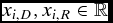 $x_{i,D},x_{i,R}\in \mathbb {R}$ such that μi − c < θ(di, xi, R), θ(xi, D, ri) < μi + c.
Proposition 1 characterizes the equilibria.
Proposition 1 Suppose that Φi is uniformly distributed on [μi − c, μi + c ], where di < μi − c < μi + c < ri. Let 0 < γ < 1. and suppose that Assumption 1 holds in district i. Then there exists ε > 0 such that, if c < ε, the following holds for all pure strategy equilibria:
1. If X < μi then the Republican wins with probability one in any pure strategy equilibrium, and the equilibrium candidate positions in district i are
(7) $$\begin{eqnarray}
&&x_{i,D} =\mu _i-c,\quad x_{i,R} = \mu _i-c \nonumber\\
&&\quad +\,\sqrt{\frac{1-\gamma }{\gamma }2 p_i(X_R-X_D)\left(\mu _i-c- X\right)}. \nonumber\\
\end{eqnarray}$$
2. If X > μi then the Democrat wins with probability one in any pure strategy equilibrium, and the equilibrium candidate positions in district i are
(8)
$$\begin{eqnarray}
&& x_{i,D} = \mu _i+c\nonumber\\
&&\quad -\,\sqrt{\frac{1-\gamma }{\gamma }2 p_i(X_R-X_D)\left(X-\mu _i-c\right)}, \nonumber\\[-12pt] \nonumber\\
&& \qquad\qquad\qquad x_{i,R}=\mu _i+c.
\end{eqnarray}$$
3. If X = μi and ri − μi = μi − di then xi, R = −xi, D = μi + ric/(ri + c), and both candidates win with equal probability.


Note first that, if national party positions differ and if no two districts have the same expected median voter positions, then either all or almost all districts are in cases 1 or 2. Consider the case that X < μi, so that type μi strictly prefers the Republican national platform over the Democratic one. In equilibrium, voter type θ who is indifferent between the two candidates must be located at μi − c, the lowest possible median voter position. Otherwise, if θ > μi − c and c is small, then the Republican candidate could increase his winning probability by a large amount by moderating slightly until the Democrat’s winning probability is zero. Also, in equilibrium, it cannot be possible for the Democrat to select a different candidate that would move θ strictly above μi − c, else, the Democrat’s winning probability would become strictly positive, making the Democrat strictly better off. In other words, for given x i, R, the function θ( ·, x i, R) assumes its maximum at x i, D, and so the first-order condition ∂θ(x i, D, x i, R)/∂x i, D = 0 must be satisfied. Using the conditions that the cutoff voter is at μi − c and that ∂θ(x i, D, x i, R)/∂x i, D = 0 implies Equation (7).
We can interpret the square root term on the right-hand side of Equation (7) as the Republican leader’s leeway in district i, in the sense that it measures the extent to which the Republican candidate can be more conservative than district i’s median voter without being too extreme and losing to the Democratic candidate.
The leeway in Equation (7) is increasing in those factors that amplify the preference of district i’s median voter for the Republican national position. First, if the Republican party position is closer to the median voter, and the median voter starts to care more about national party positions rather than local ones (i.e., γ↓), then the Republican candidate in the district can exploit this preference increase. For example, suppose that the public expects that one of the major issues in the next Congress will be filling several Supreme Court vacancies. This issue conceivably increases the importance of national party positions for voters (γ↓), relative to local candidate positions. In this environment, we would therefore expect that the ideologically advantaged party in moderately competitive districts is able to win with more extreme candidates than in the absence of such a high-stakes issue, leading to increased polarization.
Second, the more voters in a district perceive that their district might be decisive for party control in the legislature (p i↑), the more they will take their preference for the national party positions into account when choosing between local candidates. Further below, we will see that p i increases for noncentrist districts if there are fewer centrist districts, which results in more partisan candidates in the noncentrist districts.
Third, the leeway is increasing in the distance between the median voter’s preferences from the midpoint of the two party platforms. In a very moderate district, that is, one in which the median voter is close to indifferent between the parties, there is not much of an asymmetry that the local leader can exploit—if he tried too much, his party’s candidate would lose. In contrast, the favored party’s local leader in districts that are more conservative (or liberal, on the other side of the political spectrum) can force a more extreme candidate down the district median voter’s throat because the median voter is not comfortable to vote for the other party’s candidate because of his association with (locally) unpopular national positions.
Finally, the leeway is increasing in the degree of national polarization (X R − X D). This is a crucial effect, since it shows how political polarization on the national level can spill over to local races. Polarization between the two national parties renders the candidates’ party affiliations more relevant for voters and thus leads, almost everywhere, to an intensification of the respective district median voter’s party preference.
Our results are relevant for the large empirical literature that analyzes how the ideological composition of districts and, especially, the partisan gerrymandering of districts affects the ideological positions of representatives in Congress. In particular, McCarty, Poole, and Rosenthal (Reference McCarty, Poole and Rosenthal2009a, Reference McCarty, Poole and Rosenthal2009b) claim that, while Congress has become more polarized in a time during which electoral districts became more heterogeneous due to gerrymandering, this is merely a temporal coincidence. “Political scientists have demonstrated that whenever a congressional seat switches parties, the voting record of the new member is very different from that of the departing member, increasing polarization. In other words, it is becoming more common to observe a very liberal Democrat replaced by a very conservative Republican (and vice versa).” They argue that, since these switches happen in relatively competitive districts, this effect cannot be explained by gerrymandering. Further, they argue that a similar increase in polarization has been observed in the Senate that is not subject to gerrymandering, and hence gerrymandering cannot be the prime reason for increased political polarization.
An important insight from the spillover effect in our model is that this argument is somewhat flawed because the “treatment” also affects the “untreated.” Thus, if gerrymandering affects national party positions because more extreme representatives are elected from gerrymandered districts, there is also an indirect effect on the equilibrium positions of candidates in moderately competitive districts, even if these districts themselves were not directly gerrymandered. We will return to analyze this subject more closely in Proposition 4 below.
Equilibrium when National Concerns Are Dominant (γ ≈ 0)
We now turn, in this subsection and the next one, to limit cases in which we can characterize the equilibrium for an arbitrary degree of uncertainty about the median voter’s ideal position. We start with the case that all actors care primarily about national positions (γ ≈ 0).
Observe first that, when γ = 0, that is, neither voters nor party leaders care at all about their local candidates’ positions, then payoffs are independent of actions and therefore any behavior is an equilibrium. For a meaningful analysis, we therefore need to look at the case that γ is small, but positive. The following Proposition 2 shows that an equilibrium exists, and that, in districts where the median voter is, in expectation, more ideologically extreme, the winning probability of the ideologically favored party’s candidate increases.
Proposition 2 Let xi, D(γ), xi, R(γ) denote the equilibrium strategies in district i when the preference parameter is γ, and let X = (XR + XD)/2 be the voter type who is indifferent between the two national party positions. Let hi(x) = ϕi(x)/(1 − Φi(x)) be the hazard rate in district i, and suppose that Φi is symmetric around its mean μi. If γ is close to zero, then the following results hold:
1. There exists an equilibrium in which the positions of the candidates in district i are
(9)
$$\begin{eqnarray}
&&\lim _{\gamma \downarrow 0} x_{i,D}(\gamma ) = d_{i} \nonumber\\
&& \quad+\, \frac{h_i(-X+2\mu _i)(d_{i}-X)^2}{1-h_i(-X+2\mu _i)(d_{i}-X)},
\end{eqnarray}$$
(10)
$$\begin{eqnarray}
&& \lim _{\gamma \downarrow 0} x_{i,R}(\gamma ) = r_{i} \nonumber\\
&&\quad -\, \frac{h_i(X)(r_{i}-X)^2}{1+h_i(X)(r_{i}-X)}.
\end{eqnarray}$$
2. The Democratic winning probability in district i converges to Φi(X), and the Republican one to 1 − Φi(X).


The candidate positions are more moderate than the respective local party leaders’ ideal positions. The exact positions depend on the hazard rates in Equations (9) and (10), which capture the degree of uncertainty about district i’s median voter’s position, as h(t)dt is the probability that the median voter’s position is in the (small) interval [t, t + dt], conditional on being greater than t.
To illustrate Proposition 2, consider the following example where the median voter’s position follows a logistic distribution with parameter s. (The parameter s of a logistic distribution is proportional to the standard deviation of the distribution,  $s\pi /\sqrt{3}$.)
Corollary 1 Suppose that the median voter’s position is distributed logistically, with cumulative distribution given by 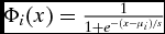 $\Phi _i(x)=\frac{1}{1+e^{-(x-\mu _i)/s}}$, so that the hazard rate is
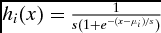 $h_i(x)= \frac{1}{s(1+e^{-(x-\mu _i)/s})}$. Then the following holds for γ close to zero:
1. Both xi, D and xi, R increase in μi.
2. Suppose that d i and r i are symmetric around X. Then increasing μi from μi = X strictly increases local polarization, that is, xi, R − xi, D increases.
3. Suppose that the expected median voter in district i has a strict preference for the Republican national party position over the Democratic one (that is, |μi − XR| < |μi − XD|). Further, suppose that the variance, s2π2/3, converges to zero. Then xi, R → ri and xi, D → X, and the Republican’s winning probability converges to 1.
4. For s > 0, changes in the national party positions XD and XR have a nonmonotone effect on the equilibrium local candidate positions xi, D and xi, R.
Proof of Corollary 1. See Appendix. ■
The first claim is very intuitive and simply means that candidates nominated in more conservative districts espouse more conservative positions.
The second claim states that polarization between the local candidates, measured as the distance between their positions, increases as the advantage of one of the parties increases. Conversely, in the most moderate district, electoral competition works best in terms of forcing both candidates toward a moderate position.
The third claim states that x i, R → r i and x i, D → X in a district where Republicans almost certainly have an ideological advantage. To get some intuition, normalize X to 0, and consider a conservative district μi > 0. Let s → 0, which means that actors become more and more confident that district i’s realized median voter in fact prefers the Republican national party position to the Democratic one, though not necessarily by much. In this case, the hazard rates in Equations (9) and (10) go to infinity and zero, respectively, which implies that x i, R → r i and x i, D → 0: Thus, both parties’ candidates choose positions that are different from the position preferred by district i’s median voter. Most significantly, the Republican candidate—who is most likely to be elected because of the median voter’s preference for the national Republican position—is at his (local) party’s ideal position.
Interestingly, the Democrats also do not choose to position their candidate at the expected median voter position μi. The reason is that, if the realized median voter is at or close to μi, the Democrats still would not win in district i, even with a local candidate close to that position competing against a relatively misaligned Republican, because the median voter’s preference for the Republican party’s national position outweighs his local candidate preference. For the Democrats to have a chance of winning in district i, the realized median voter must be close to 0 (i.e., indifferent between the national party positions), and a position near 0 is the most competitive in this contingency. In contrast to the Democratic leader, the Republican leader expects to win with a high probability in district i, so compromising by nominating a more moderate candidate is more costly in terms of expected utility, and therefore, the Republican candidate’s equilibrium position is close to r i.
Suppose that in this conservative district the median voter’s position, μi, is closer to the median primary voter’s position, r i, than to zero. Then, in addition to being disadvantaged by its national position, the Democrats may also seem “ideologically stubborn” by nominating an “inappropriate” candidate for district i. That is, if the variance is small, then the realized median voter will almost always prefer the national Republican position (over the national Democratic one) and the local Republican candidate over his Democratic challenger.
Finally, the last point in Corollary 1 considers the effect of a change in the national party positions. In general, this effect is nonmonotone, as the following thought experiment shows. Suppose that, initially, X D < 0 = X R, that is, the expected district median voter is more conservative than the national Republican position. As X R increases, the Republican advantage in district i increases, and that allows local Republicans (who have r i > μi) to nominate a more extreme candidate. As X R increases further beyond μi, the Republican advantage in district i decreases which generally (for s not too small) makes a somewhat more moderate candidate optimal for Republicans. When X R becomes large, district i starts to favor the Democratic national position (which will move x i, D toward d i), and this forces the Republican candidate toward (X D + X R)/2.
Equilibrium when Local Concerns are Dominant (γ ≈ 1)
We finally turn to the other polar case, namely that voters care primarily about the two local candidates’ positions (γ → 1). The limit case of γ = 1 is the well-known Calvert-Wittman model, so the main point of interest in this section is how a minimal voter concern about national party positions affects the parties’ strategic location incentives, relative to the Calvert-Wittman case.
Superficially, and from the results derived so far, it may seem as if voters’ national concerns should always lead to more polarization, relative to a standard Calvert-Wittman model in which each party trades off more distance from their bliss point against some gain in the probability of winning. As γ decreases from 1, the median voter’s responsiveness to local positions is lowered, and consequently nominating a candidate closer to the party’s ideal point becomes less costly.
However, nominating a more extremist candidate also becomes less attractive for the local leader because his utility also increasingly derives from national positions, and winning the local race may determine which party has the majority in the legislature. From this perspective, nominating a more moderate candidate appears more attractive, and the net effect of γ on polarization close to γ = 1 is therefore unclear. Proposition 3 analyzes this case.
Proposition 3 Consider a district where the positions of the local party leaders are symmetric around the median voter’s expected position (i.e., ri − μi = μi − di). Suppose that, starting from a situation in which all voters only care about local candidates’ positions (i.e., γ = 1), γ decreases slightly. Then, the position of the candidate of the advantaged party (i.e., the one whose national position the expected median voter prefers) moves toward μi, and the opponent’s position moves away from μi. Moreover, the first-order change in local polarization is zero, i.e.,  $\frac{\partial }{\partial \gamma }( x_{i,R}-x_{i,D})|_{\gamma =1} = 0$.
Proof. See Appendix. ■
With the symmetry assumption with respect to the two local leaders, it is easy to characterize the equilibrium of the Calvert-Wittman model. Leaders choose positions to trade off the benefit of choosing a more moderate position—an increased winning probability—with the cost of a more moderate position, namely that the policy, if the candidate wins, is farther away from the leader’s preferred position. The two candidates’ equilibrium positions are symmetric about the position of the expected median voter, and the Democrat wins if and only if the realized median voter is to the left of the expected median voter, hence with probability 1/2.
What happens when γ is now slightly decreased? For concreteness, suppose that the expected median voter in district i prefers the Democratic national position. If γ < 1 and the realized median voter is equal to the expected one, then the Democrat wins, so that the indifferent voter type is now more conservative than in the case of γ = 1. The effect on the strategic location incentives of both local leaders is as follows: For the same extent of moderation, the indifferent voter type is more responsive to movements in the Democratic candidate’s position than to that of the Republican because the indifferent voter is farther away from the Democrat’s position than from the Republican’s position.Footnote 15 Thus, the Democrat’s marginal benefit from moderation increases, and the Republican’s benefit from moderation decreases. Since the marginal cost of moderation is unchanged for both, this means that the Democratic equilibrium position will become more moderate, and the Republican one less so.
This intuition is similar to the one in Groseclose (Reference Groseclose2001), who analyzes the effect of a candidate’s valence advantage on the positions chosen by the (policy-motivated) candidates and finds that a small valence advantage induces the favored candidate to move toward the expected median voter, and the disadvantaged candidate to move away, with the latter movement being bigger so that polarization, as measured by the distance between the candidates, increases. However, there is an interesting difference: While valence in Groseclose’s model is uniformly appreciated by all voter types, the extent and even the sign of the Democrat’s net advantage varies with the preference type of the realized median voter in our model. This is the reason why the polarization result is different in our model, that is, for small changes of γ away from 1, the distance between the equilibrium Democratic and Republican position is unchanged (to the first order).
A CLOSER LOOK AT THE EFFECTS OF GERRYMANDERING
In this section, we analyze how a change in the distribution of district median voters affects the equilibrium degree of polarization, in particular in those districts that are not directly affected by the preference change. For our model, it does not matter whether the change in the district median distribution was brought about intentionally, through gerrymandering, or unintentionally through voter sorting (say, conservatives moving to conservative states, and liberals to liberal states). In the next subsection, we focus on the effect that works through affecting the pivot probabilities, and in the following subsection on the effect of endogenous party platforms.
Endogenous Pivot Probabilities
So far, we have interpreted p i, the probability with which voters in district i believe that their district is pivotal for the majority in the legislature, as an exogenously given parameter. In this section, we endogenize p i and show that this gives rise to an externality between districts. Specifically, we show that a decrease in the number of centrist districts leads to an increase in polarization.
Consider a symmetric setting with k left-leaning districts, k right-leaning districts, and 2m + 1 centrist districts. In the left-leaning and right-leaning districts, the median voters are uniformly distributed on [− μ − c, −μ + c] and [μ − c, μ + c], respectively, where μ > 0. In the centrist districts, the respective median voter is uniformly distributed on [− c, c]. Given the symmetry of the model, we assume that party positions, X D and X R are symmetric around zero, so that X = 0.Footnote 16
Proposition 1 determines the candidates’ positions and winning probabilities (when c is small). In the centrist districts, the candidates’ equilibrium positions are close to zero, independent of the pivot probability, and each candidate wins with probability 1/2. In right-leaning districts, X = 0 < μ and hence Proposition 1 implies that the Republican candidate wins. Similarly, in the left-leaning districts we have X > −μ which means that the Democrats win.
To determine the candidates’ equilibrium positions in left and right-leaning districts, we now derive the pivot probabilities, p i. Consider a particular right-leaning district. In equilibrium, all other right-leaning districts vote for Republicans and all left-leaning districts for Democrats. Given that the total number of districts is odd, the pivotal event occurs if exactly m + 1 of the centrist districts vote for the Republican candidate — in this case Republicans get m + 1 + (k − 1) legislators, excluding the selected right-leaning district, while Democrats have m + k legislators, that is, there is a tie. This occurs with probability
 $$\begin{equation}
p(m)=\left(\begin{array}{c}{2m+1}\\
{m+1}\end{array}\right)2^{-(2m+1)}.
\end{equation}$$
Note that p(m) decreases in m and, by Stirling’s formula, the pivot probability goes to zero at rate  $1/\sqrt{m}$.
Suppose we start in a situation with many centrist districts, as well as one left-leaning and one right-leaning district. Then, the pivot probabilities for the left-leaning and right-leaning districts are close to zero, and Equations (7) and (8) imply that both candidates are located close to −μ − c in the left-leaning district, and to μ + c in the right-leaning district. Hence, local political polarization (i.e., the distance between the local candidates), is small.
Now suppose that an even number of centrist districts are transformed into an equal number of left-leaning and right-leaning districts. As the number of centrist districts decreases, p i increases, and Equations (7) and (8) imply that the distance between the candidates in the left-and right-leaning districts increases, and that the advantaged candidates become more extreme. For example, if only one centrist district remains, then the pivot probability in the left and right-leaning districts increases all the way up to p i = 1/2.
Note that, in each step of removing centrist districts and transforming them into left-and right-leaning districts, the candidates become more extreme in both the newly-created districts and in those districts that were already left-leaning or right-leaning. Thus, if an empirical researcher were to “difference out the time-trend of polarization” (by looking at changes in polarization in newly-gerrymandered districts, versus existing districts), he would clearly underestimate the effects of gerrymandering.
Intuitively, in the centrist districts the electorate is willing to switch between candidates. If there are many such swing districts, then the election in the partisan district is less likely to determine the control of the legislature. As a consequence, voters in a conservative-leaning district would be more willing to give the Democratic candidate a chance, which in turn means that the Republican candidate must be relatively moderate to be competitive. If, however, there are few centrist districts, the probability that that particular district is decisive for the majority in the legislature increases. In this case, conservative voters in the same district are less likely to support the local Democratic candidate because they are more concerned that voting for him will result in Democratic control of the legislature. This, in turn, means that even a more extreme Republican candidate can win, and the Republican base can exploit this effect by nominating a more extreme candidate.
Endogenous Party Positions
So far, we have taken the national party positions as exogenous and independent of the election outcome in any specific district. Fixing the party positions may be realistic in the short run if party positions are determined by some party elite that the individual representative cannot influence, or because, even if the party position is jointly decided by the party’s elected legislators, the party position that voters perceive at the time of the election is unlikely to be conditional on the outcome of the election in the district in question. In the long run, though, it is useful to consider a situation in which a party’s position is an aggregate of the positions of its winning candidates.
We interpret X R and X D as the party policies that voters expect to be implemented if the respective parties win a majority. It is plausible that these expected policies are a function of the positions of the individual candidates, weighted by their respective probability of getting elected. For example, a Democratic candidate in Utah who has an extremely small chance of being elected probably has a much smaller impact on the perception of the Democratic position in the rest of the country than a candidate from the urban Northeast, who is almost certain to be elected.
To formalize this notion, we need a bit of notation. Let x L, D and x C, D be the positions of the Democratic candidates in the left-leaning and centrist districts, respectively. Similarly, let x C, R, and x R, R be the positions of the Republican candidates in centrist and right-leaning districts. We assume that the party positions are a weighted sum of the positions of representatives from these districts, that is,
 $$\begin{eqnarray}
X_R &=& \alpha (k,m) x_{R,R}+(1-\alpha (k,m))x_{C,R}, \nonumber\\
X_D &=& \alpha (k,m) x_{L,D}+(1-\alpha (k,m))x_{C,D},
\end{eqnarray}$$
where α(k, m) is decreasing in m (i.e., the expected number of representatives from centrist districts) and increasing in k, the number of representatives from more partisan districts. Note that because Republicans are elected with zero probability in left-leaning districts, the positions of these candidates do not affect X R. Similarly, X D does not depend on the position of Democratic candidates who run in right-leaning districts and lose with probability one. For example, if the weights are solely determined by the probability of getting elected then α = k/(k + m + 1/2).Footnote 17Note that Equation (12) implies that X D = −X R. Thus, Proposition 1 implies
 $$\begin{eqnarray*}
&& x_{i,R} = \mu -c\\
&& \quad+\,2\sqrt{\frac{1-\gamma }{\gamma }\left(\alpha (k,m) x_{i,R}+(1-\alpha (k,m))\frac{rc}{r+c}\right)\left(\mu -c- X\right)},
\end{eqnarray*}$$
Solving this equation for x i, R yields
 $$\begin{eqnarray}
&& x_{i,R} =( \mu -c)\bigl (1+2\alpha a p\bigr ) \nonumber\\
&& \quad +\, 2\sqrt{ap(\mu -c)\left(\left(\alpha +ap\alpha ^2\right)(\mu -c) +(1-\alpha )\frac{rc}{r+c}\right)},\nonumber\\
\end{eqnarray}$$
where a = (1 − γ)/γ, α = α(k, m) and p = p(m).Footnote 18
Now suppose again that some centrist districts are transformed into more partisan ones (m↓, k↑). Then α(k, m) increases. The previous subsection showed that p(m) increases. Equation (13) immediately implies that x i, R increases. This is summarized formally in Proposition 4.
Proposition 4 Suppose there are 2m + 1 centrist districts, k left-leaning, and k right-leaning district in which Φi are uniform distributions, and Assumption 1 holds. Further, assume that the position of the local leaders is the same in all districts, and that the national party positions are given by a weighted sum of the positions of the Democratic and Republican legislators, respectively. Suppose that k is increased and m decreased. Then:
1. The positions of all candidates in the left-leaning and right-leaning districts become more extreme.
2. Local polarization, xi, R − xi, D in left and right-leaning districts increases;
3. Party polarization, XR − XD, increases.
In summary, the results of this section show two channels through which a change in the distribution of district medians can affect local and society-wide polarization. First, a reduction in the number of swing districts increases the pivot probability in each district, and thereby makes it easier for more extreme candidates to win in competitive districts that lean either liberal or conservative. Second, a reduction in the number of swing districts implies that each party has fewer members from moderate districts in their caucus, and this shifts the perceived position of each party to be more extreme. This, in turn, again increases the local party leaders’ leeway to nominate more extreme candidates in ideologically favorable, but (in principle) competitive districts.
EMPIRICAL IMPLICATIONS
We now discuss some evidence regarding two empirical predictions of our model.
Partisanship in Legislative and Executive Elections
Our model presumes that, in legislative elections, voters care not only about the positions of their local candidates, but also about those of the national parties. In contrast, in elections for executive positions, the winner is much freer to implement his position and, consequently, his association with a party matters less. Thus, voters’ ideological preferences should have a much larger effect in legislative elections than in executive ones.
To analyze this prediction, we consider Gubernatorial and U.S. Senate elections from 1978 to 2012. While both of these types of contests are high-profile, statewide races, gubernatorial elections are for executive positions while Senate elections are for legislative ones. Consistent with the empirical literature, we measure the median state ideology by its Partisan Voting Index (PVI), that is, the difference of the state’s average Republican and Democratic Party’s vote share in the past U.S. Presidential election, relative to the nation’s average share of the same.Footnote 19 The dependent variable is the difference between the Democrat’s and the Republican’s share of the two party vote in a particular election. In addition to the main independent variables of interest (PVI and PVI ×Senate election), we use incumbency and election type (i.e., Senate or governor election) dummies and year fixed effects to control for the electoral advantage of incumbents, and for election-cycle national shocks in favor of one party.
Table 1 summarizes the results, with the first column (all years since 1978, all states) as the baseline case. For Gubernatorial elections, the omitted category, the PVI coefficient indicates that a one point increase in the Democratic vote share in Presidential elections increases the Democratic gubernatorial candidate’s vote share only by about 0.591 points. In contrast, in Senate elections, the same ideological shift increases the Democratic Senate candidate’s vote share by 0.591 + 0.457 = 1.048 points. Evidently, the difference between executive and legislative elections is substantial and highly significant. The remaining three columns confirm the qualitative robustness of this difference if we restrict to elections after 1990 and if we exclude the political South.Footnote 20
Senate and Gubernatorial Elections

*** indicates significance at the 1% level. Data Source: Congressional Quarterly, http://library.cqpress.com/elections/
District Preferences, Representatives’ Positions, and Election Results
In districts where the candidates face effective competition, the leader of the ideologically advantaged party is constrained in the sense that he cannot choose his own ideal candidate, because such a relatively extreme candidate would be vulnerable to a challenge by a moderate candidate from the other party. Within this competitive range, a move toward a slightly more conservative district has a relatively large marginal effect on the representative’s position. To see this formally, differentiate Equation (7) with respect to μi to yield
 $$\begin{equation}
\frac{\partial x_{i,R}}{\partial \mu _i}=1+ \sqrt{\frac{p_i \frac{1-\gamma }{\gamma } (X_R-X_D) }{2\left(\mu _i-c- X\right)}}.
\end{equation}$$
Thus, moving the district median to the right by one unit, moves the position of the Republican candidate by more than one unit. An analogous result for x i, D obtains from differentiating Equation (8) with respect to μi.
In contrast, in extreme districts where Assumption 1 is violated, the advantaged party is no longer constrained by the candidate nominated by the other party. As a consequence, local party leaders nominate a candidate at their ideal point. Thus, changing μi has no direct effect on the winning candidate’s position.
To test the prediction that changes in μi have a larger effect in moderate districts than in extreme districts, we focus on open seat House elections from 1990 to 2010 (102nd to 112th Congress). This gives us 487 observations, for which we first estimate a simple probit model with electing a Democrat as the dependent variable, and the district PVI as the explanatory variable. This gives us, for every district-year combination, an estimate of the probability of electing a Democrat. When this estimated probability is larger than 80% , we consider the district as “safe” for Democrats; when it is below 20% , we consider it as safe for Republicans, and the remaining ones are nonsecure. With this definition, there are 123 safe Republican districts, 100 safe Democratic districts, and 264 district-year combinations in which an open seat race is competitive, of which 156 are won by Republicans and 108 by Democrats.Footnote 21
For each of the four groups of districts, we then regress the elected representative’s DW-Nominate score (times 100), a standard ideological position measure (Poole and Rosenthal Reference Poole and Rosenthal2000), on the district PVI at the time of the election. The results are shown in Table 2.
The Relationship between Democratic and Republican DW-Nominate Scores and District PVI in Secure (80%+) and Nonsecure Districts

*** indicates significance at the 1% level, ** at the 5% level, * at the 10% level.
Consistent with the model, the marginal effect of a change in the PVI on the representative’s DW-Nominate score is considerably weaker in secure districts than in nonsecure districts. Indeed, in secure Republican districts, the marginal effect is not significantly different from zero. On the Democratic side, the effect in secure districts is positive and significant, but considerably smaller than the effect in nonsecure districts.
Note that a heuristic alternative theory to our model, along the lines of Lupia and McCubbins (Reference Lupia and McCubbins1998) and Hinich and Munger (Reference Hinich and Munger1994), is that voters care about national party positions because they do not actually observe their local candidates’ positions, while they are better informed about national party positions. Such an informational theory is consistent with parties being sure to win in districts that are ideologically closer to their national position, independent of the position of their local candidate. However, if voters cannot observe the positions of local candidates, then parties would, in every district, run candidates located at their ideal positions (as moderation does not pay if it is not observed by voters). Thus, this theory is inconsistent with the findings reported in Table 2, which indicate that candidate positions, at least in the competitive district range, do respond to a district’s ideological leanings.
Finally, our model also generates predictions on the relationship between district ideology and winning margin in the district. In moderate districts (where Assumption 1 holds), the leader of the favored party optimally exploits a marginally more favorable electorate composition by nominating a marginally more extreme candidate. If the degree of uncertainty about the median voter position is small, the winning margin in all moderate districts (where the party leader is constrained) is small. However, in districts where the leader of the advantaged party is unconstrained (i.e., Assumption 1 is violated), the winning margin increases when moving to a marginally more extreme district.
This is exactly the empirical pattern that Winer, Kenny, and Grofman (Reference Winer, Kenny and Grofman2014) find for U.S. Senate elections between 1922 and 2004: For a range of moderate states (i.e., a range of states with a PVI relatively close to zero), the estimated marginal effect of a state’s PVI on the vote difference between Democrats and Republicans is close to zero, while this marginal effect is much larger for states that are outside this range.
CONCLUSION
Much of the existing literature on electoral competition in legislative elections implicitly assumes that voters evaluate their local candidates based only on their own positions, but not on the party label under which they run. Such a model implies that both parties nominate candidates who are very close to the preferences of the respective district median voters. Therefore, even in districts with rather extreme preferences, both parties’ candidates should be competitive, and the position of Democratic and Republican Congressmen elected from similar districts should be very similar. It is safe to say that these predictions are not borne out in reality, and to understand why this is the case is of first-order importance for our understanding of the American democratic system.
In this paper, we have developed a theory of electoral competition in a world where majority party legislators collaboratively influence policy and voters therefore rationally care about candidates’ party labels. This model yields results that are fundamentally different from the standard model.
In our model, a candidate’s association with candidates of the same party that run in other districts generates an incentive for voters to focus less on the candidates’ own position when deciding whom to vote for—local candidates are “contaminated” by their party association. This leads to less competitive local elections, providing the ideologically favored party with the leeway to nominate more extreme candidates who are nevertheless elected. As a consequence, the equilibrium of our model can explain how spillovers from electoral competition in other districts can beget a very polarized legislature.
Our analysis has three additional important empirical implications. First, it can explain why a district’s ideological preferences have a smaller partisan effect in elections in which a candidate has a more autonomous policy influence, such as elections for executive leadership positions than in legislative elections. Of course, in reality, even executive leader positions are not entirely autonomous, so there will be some contamination in executive elections as well, but we would expect this effect to be smaller than in legislative elections, and this expectation is borne out in our empirical analysis of Senate and gubernatorial elections.
Second, our model predicts that in ideologically relatively moderate districts, the marginal effect of a district becoming slightly more extreme on the district representative’s position is large, while the effect on the vote share in the general election is small. The reverse marginal effects arise in ideologically more extreme districts. These effects arise in our model because of the behavior of the primary voters of the party whose national position is more popular in the district: A marginal ideology shift in competitive districts is exploited through the nomination of a more partisan candidate while, in noncompetitive districts, the primary voters already nominate their ideal candidate, and an ideology shift in the general election electorate just means that the favored party’s candidate wins with a larger vote share. We find empirical evidence for these predictions.
Third, much of the existing empirical analysis of the effects of gerrymandering on polarization in Congress is implicitly based on applying a naive model in which voters care only about the local candidates’ positions. Such a model may lead to incorrect inferences about the importance of gerrymandering. For example, one cannot infer that gerrymandering does not matter for polarization in Congress from showing that there is no marginal effect of changes in district medians on ideological positions of legislators, and that the difference in voting records of Republicans and Democrats representing the same or very similar districts has increased. In general, an implication of our model for empirical work is that legislator behavior in different districts is intricately connected rather than independent, and this implies that one needs to be very careful with claims that difference-in-difference approaches can identify causation.
APPENDIX
Proof of Proposition 1. Without loss of generality, normalize the distribution of median voters such that it is centered around 0, that is, we have a uniform distribution on [− c, c]. Let X < 0. Then X = (X D + X R)/2 < −c for small c. Let a = (1 − γ)/γ. Let θ be the type who is indifferent between the candidates. Then Equation (3) implies that
 $$\begin{eqnarray}
\frac{\partial \theta (x_{i,D},x_{i,R})}{\partial x_{i,D}} = \frac{(x_{i,R}-x_{i,D})^2-2 p_i a(X_R-X_D)(x_{i,D}- X)}{2\left(p_ia(X_R-X_D)+x_{i,R}-x_{i,D}\right)^2}; \nonumber\\
\end{eqnarray}$$
 $$\begin{eqnarray}
\frac{\partial \theta (x_{i,D},x_{i,R})}{\partial x_{i,R}} & = & \frac{(x_{i,R}-x_{i,D})^2+2 p_i a(X_R-X_D)(x_{i,R}- X)}{2\left(p_ia(X_R-X_D)+x_{i,R}-x_{i,D}\right)^2}.\nonumber\\
\end{eqnarray}$$
If x i, D ∈ [− c, c] and x i, R > c, then Equation (16) and the fact that X < −c and imply that ∂θ(x i, D, x i, R)/∂x i, R > 0. If −c < θ(x i, D, x i, R) < c then the first-order condition Equation (40) in the proof of Proposition 3 applies. Because x i, R > x i, D > d i and X R > X D > d i this implies that the first summand in Equation (40) is strictly negative. If c is small, then ϕ(θ) = 1/(2c) becomes large, and hence the first summand of Equation (40) dominates the second summand. Hence, the left-hand side of Equation (40) is strictly negative, that is, it is optimal to lower x i, R. Thus, in equilibrium θ(x i, D, x i, R) = −c, so that the winning probability of the Republican candidate is 1.
Next,
 $$\begin{eqnarray}
&& \frac{\partial \theta ^2(x_{i,D},x_{i,R})}{\partial x_{i,D}^2} \nonumber\\
&& \quad = -\frac{2p_ia(X_R-X_D)\left(p_i(X_R-X_D)+2(x_{i,R}- X)\right)}{\left(p_ia(X_R-X_D)+x_{i,R}-x_{i,D}\right)^3}<0. \nonumber\\
\end{eqnarray}$$
Thus, in a pure strategy equilibrium x i, D and x i, R must satisfy both ∂θ(x i, D, x i, R)/∂x i, D = 0 and θ(x i, D, x i, R) = −c.
In particular, if  $\partial \theta (x_{i,D},x_{i,R})/\partial x_{i,D}\not=0$ then an appropriate change of x i, D would raise θ(x i, D, x i, R) and hence the Democrat’s winning probability would become strictly positive. If ∂θ(x i, D, x i, R)/∂x i, D = 0 then strict concavity of θ(x i, D, x i, R) in x i, D, established in Equation (17) implies that any change of x i, D would lower the position of the cutoff voter θ(x i, D, x i, R) and hence the winning probability of the Democratic candidate remains at zero.
If the distribution, instead of being centered at 0, is centered at μi the following two conditions must be satisfied: ∂θ(x i, D, x i, R)/∂x i, D = 0 and θ(x i, D, x i, R) = μi − c.
Note that Equation (15) implies that ∂θ(x i, D, x i, R)/∂x i, D = 0 if and only if −x i, D + θ(x i, D, x i, R) = 0. Thus, x i, D = μi − c. Next, solving Equation (16) for x i, R and using the fact that x i, D = μi − c yields Equation (7). The derivation of Equation (8) is similar.
The case where X > 0 symmetric. Thus, assume that X = 0. Taking the derivative with respect to x i, R of Equation (32) and substituting x i, D = −x i, R, we get
 $$\begin{eqnarray*}
\frac{\partial \theta (x_{i,D},x_{i,R})}{\partial x_{i,R}} = \frac{X_R}{2ap_i X_R+2x_{i,R}}.
\end{eqnarray*}$$
Substituting this into the Republican’s first-order condition Equation (40) and using that x i, D = −x i, R implies that x i, R = r ic/(r i + c). By symmetry, the first-order condition of the Democrat is also satisfied. It is easy to check that the second-order condition holds and that this is the unique equilibrium. ■
Proof of Proposition 2. First suppose that μi = 0.
The cutoff voter, who is indifferent between the candidates, is given by Equation (3). Note that
 $$\begin{eqnarray}
&& \lim _{\gamma \rightarrow 0}\frac{1}{\gamma }\frac{\partial \theta (x_{i,D},x_{i,R})}{\partial x_{i,D}}=\frac{X_R+X_D-2x_{i,D}}{2p_i (X_R-X_D)}, \nonumber\\
&& \text{ \ and \ } \lim _{\gamma \rightarrow 0} \theta (x_{i,D},x_{i,R})= \frac{X_D+X_R}{2}.
\end{eqnarray}$$
Thus, the the winning probability of the Democrat converges to Φi(X) as γ becomes small. The winning probability of the Republican candidate converges to 1 − Φi(X), where X = (X D + X R)/2.
The Democratic primary voter solves Equation (4). The first-order condition is
 $$\begin{eqnarray}
&& -\phi _i(\theta )\frac{\partial \theta (x_{i,D},x_{i,R})}{\partial x_{i,D}} \Big( \gamma \bigl ((x_{i,D}-d_{i})^2-(x_{i,R}-d_{i})^2\bigr )\nonumber\\
&&\quad +\,(1-\gamma )p_i\bigl ((X_D-d_{i})^2 -(X_R-d_{i})^2\bigr ) \Big) \nonumber\\
&&\quad -\,2\Phi _i(\theta )\gamma \bigl (x_{i,D}-d_{i}\bigr ) = 0.
\end{eqnarray}$$
Dividing Equation (19) by γ, then taking the limit for γ → 0, using Equation (18), and the fact that Φi is symmetric, yields
 $$\begin{eqnarray}
&&\phi _i\left( \frac{X_D+X_R}{2}\right)\frac{X_R+X_D-2x_{i,D}}{2 (X_R-X_D)}\nonumber\\
&&\quad\times\,\Bigl ((X_R-d_{i})^2 -(X_D-d_{i})^2 \Bigr )\nonumber\\
&&\quad=2\Phi _i\left( \frac{X_D+X_R}{2}\right)\bigl (x_{i,D}-d_{i}\bigr ).
\end{eqnarray}$$
Next,
 $$\begin{equation}
\lim _{\gamma \rightarrow 0}\frac{1}{\gamma }\frac{\partial \theta (x_{i,D},x_{i,R})}{\partial x_{i,R}}=\frac{2x_{i,R}-(X_R+X_D)}{2p_i (X_R-X_D)}.
\end{equation}$$
The Republican primary solves Equation (5). The first-order condition is
 $$\begin{eqnarray}
&&-\phi _i(\theta )\frac{\partial \theta (x_{i,D},x_{i,R})}{\partial x_{i,R}} \Big( \gamma \bigl ((x_{i,D}-r_{i})^2-(x_{i,R}-r_{i})^2\bigr )\nonumber\\
&&\quad +\,(1-\gamma )p_i\bigl ((X_D-r_{i})^2 -(X_R-r_{i})^2\bigr ) \Big) \nonumber\\
&&\quad +\,2\gamma \left(1-\Phi _i(\theta )\right)(r_{i}-x_{i,R}) = 0.
\end{eqnarray}$$
Again, dividing by γ, setting γ = 0 and using the fact that θ = 0 when γ = 0, yields
 $$\begin{eqnarray}
&&\phi _i\left(- \frac{X_D+X_R}{2}\right)\frac{2x_{i,R}-(X_R+X_D)}{2 (X_R-X_D)} \nonumber\\
&&\quad \times\,\Bigl ((X_D-r_{i})^2 -(X_R-r_{i})^2 \Bigr )\nonumber\\
&&\qquad =2\Phi _i\left(- \frac{X_D+X_R}{2}\right)(r_{i}-x_{i,R}) .
\end{eqnarray}$$
Note that h(x) = ϕi(x)/(1 − Φi(x)) is the hazard rate of the distribution Φi. The symmetry of the distribution implies h(x) = ϕi(x)/Φi( − x) = ϕi( − x)/Φi( − x). Solving Equation (20) for x i, D yields
 $$\begin{eqnarray}
&& x_{i,D} =\frac{1}{2} \nonumber\\
&&\quad \times\,\frac{ -h\left(- \frac{X_D+X_R}{2}\right)(X_R+X_D)^2 + 2h\left(- \frac{X_D+X_R}{2}\right)d_{i}(X_D+X_R)-4d_{i} }{-h\left( \frac{-X_D+X_R}{2}\right)(X_D+X_R)+2h\left(- \frac{X_D+X_R}{2}\right)d_{i}-2}.\nonumber\\
\end{eqnarray}$$
Similarly, Equation (23) implies
 $$\begin{eqnarray}
&& x_{i,R} =\frac{1}{2} \nonumber\\
&&\quad\times\,\frac{ -h\left( \frac{X_D+X_R}{2}\right)(X_R+X_D)^2 + 2h\left( \frac{X_D+X_R}{2}\right)r_{i}(X_D+X_R)+4r_{i} }{-h\left( \frac{X_D+X_R}{2}\right)(X_D+X_R)+2h\left( \frac{X_D+X_R}{2}\right)r_{i}+2}. \nonumber\\
\end{eqnarray}$$
Let X = (X D + X R)/2. Then Equations (24) and (25) can be written as
 $$\begin{equation}
x_{i,D} & = & d_{i} + \frac{h_i(-X)(d_{i}-X)^2}{1-h_i(-X)(d_{i}-X)},
\end{equation}$$\\
 $$\begin{equation}
x_{i,R} & = & r_{i} - \frac{h_i(X)(r_{i}-X)^2}{1+h_i(X)(r_{i}-X)}.
\end{equation}$$
 $$\begin{eqnarray}
&&-\left(\phi _i(\theta )\frac{\partial ^2 \theta (x_{i,D},x_{i,R})}{\partial x_{i,D}^2}+\phi _i^{\prime }(\theta )\left(\frac{\partial \theta (x_{i,D},x_{i,R})}{\partial x_{i,D}}\right)^2\right) \nonumber\\
&& \quad \cdot \Big(\gamma \left( (x_{i,D}-d_{i})^2 -(x_{R,i}-d_{i})^2 \right)\nonumber\\
&&\qquad +\,(1-\gamma )p_i\bigl ((X_D-d_{i})^2 -(X_R-d_{i})^2\bigr )\Big) \nonumber\\
&&\qquad -\,4\gamma \phi _i(\theta )\frac{\partial \theta (x_{i,D},x_{i,R})}{\partial x_{i,D}}(x_{i,D}-d_{i})-2\gamma \Phi _i(\theta ).
\end{eqnarray}$$
Note that
 $$\begin{eqnarray}
&&\lim _{\gamma \rightarrow 0}\frac{\partial ^2 \theta (x_{i,D},x_{i,R})}{\partial x_{i,D}^2} \frac{1}{\gamma } = -\frac{1}{p_i (X_R-X_D)}, \nonumber\\
&&\quad \text{and \ } \lim _{\gamma \rightarrow 0}\left(\frac{\partial \theta (x_{i,D},x_{i,R})}{\partial x_{i,D}}\right)^2\frac{1}{\gamma } =0.
\end{eqnarray}$$
Dividing Equation (28) by γ, taking the limit for γ → 0, and using Equations (18) and (29) yields
 $$\begin{eqnarray*}
&&-\frac{\phi _i\left(\frac{X_D+X_R}{2}\right)\bigl ((X_R-d_{i})^2 -(X_D-d_{i})^2\bigr )}{X_R-X_D} \nonumber\\
&&\quad -\,2\Phi _i\left(\frac{X_D+X_R}{2}\right)<0.
\end{eqnarray*}$$
Thus, for small γ the objective is concave for all x i, D. Concavity of the Republican’s objective follows similarly. Hence, Equations (26) and (27) describe the Nash equilibrium of the game when μi = 0.
Now suppose that μi is arbitrary. Let  $\tilde{X}=X-\mu _i$,
 $\tilde{d}_i=d_i-\mu _i$, and
 $\tilde{r}_i=r_i-\mu _i$, that is, we shift all parameters by −μi.
By assumption, Φi(x) is symmetric around μi. Thus, Φi(x + μi) is symmetric around zero. Let  $\tilde{h}(x)$ be the hazard rate of the distribution Φi(x + μi). Thus,
 $\tilde{h}(x)=h(x+\mu _i)$. Finally, et
 $\tilde{x}_{i,D}$ and
 $\tilde{x}_{i,R}$ be the candidate position in the model shifted by μi. We can now apply Equations (26) and (27) to get
 $$\begin{eqnarray*}
\lim _{\gamma \downarrow 0} \tilde{x}_{i,D}(\gamma )& = \tilde{d}_{i} + \frac{\tilde{h}_i(-X)(\tilde{d}_{i}-\tilde{X})^2}{1-\tilde{h}_i(-\tilde{X})(\tilde{d}_{i}-\tilde{X})},\\
\lim _{\gamma \downarrow 0} \tilde{x}_{i,R}(\gamma ) &=r_{i} - \frac{\tilde{h}_i(X)(\tilde{r}_{i}-X)^2}{1+\tilde{h}_i(X)(\tilde{r}_{i}-\tilde{X})}.
\end{eqnarray*}$$
Further, note that the equilibrium candidate positions must also be shifted by μi. Thus,  $\tilde{x}_{i,P}=x_{i,P}-\mu _i$, for P = D, R. Substituting these values into the above equations yields
 $$\begin{eqnarray*}
\lim _{\gamma \downarrow 0} x_{i,D}(\gamma )-\mu _i& = d_{i}-\mu _i + \frac{\tilde{h}_i(-X+\mu _i)(d_{i}-X)^2}{1-\tilde{h}_i(-\tilde{X}+\mu _i)(d_{i}-X)},\\
\lim _{\gamma \downarrow 0} x_{i,R}(\gamma )-\mu _i &=r_{i} -\mu _i- \frac{\tilde{h}_i(X-\mu _i)(r_{i}-X)^2}{1+\tilde{h}_i(X-\mu _i)(r_{i}-X)}.
\end{eqnarray*}$$
Note that  $\tilde{h}_i(-X+\mu _i)=h_i(-X+2\mu _i)$. Further,
 $\tilde{h}_i(X-\mu _i)=h(X)$. This implies Equations (9) and (10). ■
Proof of Corollary 1. Substituting the hazard rate of the logistical distribution into Equations (9) and (10) yields
 $$\begin{equation}
\lim _{\gamma \downarrow 0} x_{i,D}(\gamma ) & = & \frac{d_i s e^{\frac{X-\mu _i}{s}}-(X-s)d+X^2}{s e^{\frac{X-\mu _i}{s}}+X-d_i+s},
\end{equation}$$\\
 $$\begin{equation}
\lim _{\gamma \downarrow 0} x_{i,R}(\gamma )& = & \frac{r_i s e^{\frac{-X+\mu _i}{s}}+(X+s)r_i-X^2}{s e^{\frac{-X+\mu _i}{s}}-X+r_i+s}.
\end{equation}$$
If r i and d i are symmetric around X we can renormalize the policy line such that r i = −d i and X = 0. Then the derivative of the right-hand side of Equation (31) minus the right-hand side of Equation (30) is
 $$\begin{eqnarray*}
\frac{(2s+r_i)r_i^3e^{\frac{\mu _i}{s}}\left(e^{\frac{2\mu _i}{s}}-1\right)}{ \left(se^{\frac{\mu _i}{s}}+r_i+s\right)^2\left((r_i+s)e^{\frac{\mu _i}{s}}+s\right)^2 }>0.
\end{eqnarray*}$$
Thus, if γ is close to zero, then raising μi and thus giving the Republican candidate an advantage strictly increases polarization x i, R(γ) − x i, D(γ).
If s↓0 then hazard rate h i(x) converges to 0 if x < μi. Otherwise, if x > μi then h i(x) goes to infinity. Suppose that X < μi. Then −X + 2μi > μi. Hence, h i( − X + 2μi) goes to infinity as s↓0. Thus, Equation (30) implies that limγ↓0x i, D = X. Further, X < μi implies that h i(X) converges to zero, and therefore Equation (31) implies limγ↓0x i, D = d i. The result for X > μi are analogous. ■
Proof of Proposition 3. In the following, we assume that r i = −d i. Let  $a=\frac{1-\gamma }{\gamma }$. Let x i, R(a) and x i, D(a) be the optimal policy choices given a ⩾ 0. If a = 0 then party policies are irrelevant. Thus, r i = −d i implies that x i, R(0) = −x i, D(0). This implies that θ(x i, D(0), x i, R(0)) = 0.
Then
 $$\begin{equation}
\theta (x_{i,D},x_{i,R})=\frac{1}{2} \frac{ ap_i(X_R^2-X_D^2)+(x_{i,R}^2-x_{i,D}^2)}{ ap_i(X_R-X_D)+(x_{i,R}-x_{i,D})}.
\end{equation}$$
Then
 $$\begin{equation}
\frac{\partial \theta (x_{i,D}(a),x_{i,R}(a))}{\partial a}\biggr |_{a=0}= \frac{x_{i,D}^{\prime }(0)+x_{i,R}^{\prime }(0)}{2}+ \frac{p_i(X_R^2-X_D^2)}{4x_{i,R}(0)}.
\end{equation}$$
Further,
 $$\begin{eqnarray}
&& \frac{\partial }{\partial a} \left(\frac{\partial \theta }{\partial x_{i,D}}(x_{i,D}(a),x_{i,R}(a))\right)\biggr |_{a=0} \nonumber\\
&&\quad = \frac{p_i\Bigl ( X_R^2-X_D^2-2x_{i,R}(0)(X_R-X_D)\Bigr )}{8x_{i,R}(0)^2},
\end{eqnarray}$$
 $$\begin{eqnarray}
&& \frac{\partial }{\partial a} \left(\frac{\partial \theta }{\partial x_{i,R}}(x_{i,D}(a),x_{i,R}(a))\right)\biggr |_{a=0} \nonumber\\
&&\quad = - \frac{p_i\Bigl ( X_R^2-X_D^2+2x_{i,R}(0)(X_R-X_D)\Bigr )}{8x_{i,R}(0)^2}.
\end{eqnarray}$$
Finally,
 $$\begin{equation}
\frac{\partial \theta (x_{i,D}(0),x_{i,R}(0))}{\partial x_{i,D}}=\frac{\partial \theta (x_{i,D}(0),x_{i,R}(0))}{\partial x_{i,R}}=\frac{1}{2}.
\end{equation}$$
The optimal policies must satisfy the Democratic primary voter’s first-order condition
 $$\begin{eqnarray}
&& -\phi _i(\theta )\frac{\partial \theta (x_{i,D},x_{i,R})}{\partial x_{i,D}} \Big( \bigl ((x_{i,D}(a)-d_{i})^2-(x_{i,R}(a)-d_{i})^2\bigr )\nonumber\\
&&\quad +\, ap_i\bigl ((X_D-d_{i})^2 -(X_R-d_{i})^2\bigr ) \Big) \nonumber\\
&&\quad -\, 2\Phi _i(\theta )\bigl (x_{i,D}(a)-d_{i}\bigr ) = 0.
\end{eqnarray}$$
We now take the derivative of Equation (37) with respect to a at a = 0. Note that θ(x i, D(0), x i, R(0)) = 0 and the symmetry of the distribution Φi implies that ϕ′i(θ(x i, D(0), x i, R(0))) = 0. We therefore get
 $$\begin{eqnarray}
&&-\phi _i(0)\frac{\partial }{\partial a} \left(\frac{\partial \theta }{\partial x_{i,D}}(x_{i,D}(a),x_{i,R}(a))\right) \biggr |_{a=0} \nonumber\\
&&\quad \times\,\left((x_{i,D}(0)-d_{i})^2-(x_{i,R}(0)-d_{i})^2\right) \nonumber\\
&& -\phi _i(0)\frac{\partial \theta (x_{i,D}(0),x_{i,R}(0))}{\partial x_{i,D}}\big(2(x_{i,D}(0)-d_{i})x_{i,D}^{\prime }(0)\nonumber\\
&&\quad -\,2(x_{i,R}(0)-d_{i})x_{i,R}^{\prime }(0)+p_i\bigl ((X_D-d_{i})^2 -(X_R-d_{i})^2\bigr ) \big)\nonumber\\
&&-2\phi _i(0)\frac{\partial \theta (x_{i,D}(a),x_{i,R}(a))}{\partial a} \biggr |_{a=0}\bigl (x_{i,D}(a)-d_{i}\bigr ) -2\Phi _i(0)x_{i,D}^{\prime }(0) = 0. \nonumber\\
\end{eqnarray}$$
Substituting Equations (33), (34), and (36) into Equation (38) and using the fact that x i, R(0) = −x i, D(0) yields
 $$\begin{eqnarray*}
&&-\frac{\phi _i(0)p_id_i\Bigl ( X_R^2-X_D^2-2x_{i,R}(0)(X_R-X_D)\Bigr )}{2x_{i,R}(0)} \\
&&\qquad -\,\frac{\phi _i(0)}{2}\Big(2(x_{i,D}(0)-d_{i})x_{i,D}^{\prime }(0)-2(x_{i,R}(0)-d_{i})x_{i,R}^{\prime }(0) \nonumber\\
&&\qquad \quad +\, p_i\bigl ((X_D-d_{i})^2 -(X_R-d_{i})^2\bigr ) \Big) \\
&&\qquad -\,2\phi _i(0)\left(\frac{x_{i,D}^{\prime }(0)+x_{i,R}^{\prime }(0)}{2}+ \frac{p_i(X_R^2-X_D^2)}{4x_{i,R}(0)}\right)\nonumber\\
&&\qquad \quad \times\,\bigl (x_{i,D}(0)-d_{i}\bigr ) -x_{i,D}^{\prime }(0) = 0,
\end{eqnarray*}$$
which is equivalent to
 $$\begin{eqnarray}
&& \phi _i(0)p_i\Bigl ( X_R^2-X_D^2\Bigr )-\Bigl (1+2\phi _i(0)(r_i-x_{i,R}(0))\Bigr )x_{i,D}^{\prime }(0)\nonumber\\
&&\quad +\,2\phi _i(0)x_{i,R}(0)x_{i,R}^{\prime }(0)=0.
\end{eqnarray}$$
The optimal policies must also satisfy the Republican’s first-order condition; that is,
 $$\begin{eqnarray}
&& -\phi _i(\theta )\frac{\partial \theta (x_{i,D}(a),x_{i,R}(a))}{\partial x_{i,R}}\nonumber\\
&&\quad \times\, \Big(\bigl ((x_{i,D}(a)-r_{i})^2-(x_{i,R}(a)-r_{i})^2\bigr ) \nonumber\\
&&\quad +\,ap_i\bigl ((X_D-r_{i})^2 -(X_R-r_{i})^2\bigr ) \Big) \nonumber\\
&&\quad +\,2\left(1-\Phi _i(\theta )\right)(r_{i}-x_{i,R}(a)) = 0.
\end{eqnarray}$$
The derivative of Equation (40) with respect to a at a = 0 is
 $$\begin{eqnarray}
&&-\phi _i(0) \frac{\partial }{\partial a} \left(\frac{\partial \theta }{\partial x_{i,R}}(x_{i,D}(a),x_{i,R}(a))\right)\biggr |_{a=0} \nonumber\\
&&\qquad\times\,\left((x_{i,D}(0)-r_{i})^2-(x_{i,R}(0)-r_{i})^2\right) \nonumber\\
&&\qquad-\phi _i(0)\frac{\partial \theta (x_{i,D}(0),x_{i,R}(0))}{\partial x_{i,R}}\big(2(x_{i,D}(0)-r_{i})x_{i,D}^{\prime }(0)\nonumber\\
&&\qquad - 2(x_{i,R}(0)-r_{i})x_{i,R}^{\prime }(0)\nonumber\\
&&\quad +\,p_i\bigl ((X_D-r_{i})^2 -(X_R-r_{i})^2\bigr )\big) \nonumber\\
&&\quad -\, 2\phi _i(0)\frac{\partial \theta (x_{i,D}(a),x_{i,R}(a))}{\partial a}\biggr |_{a=0}\bigl (r_i-x_{i,R}(a)\bigr ) \nonumber\\
&&\qquad -\, 2\left(1-\Phi _i(0)\right)x_{i,R}^{\prime }(0) = 0.
\end{eqnarray}$$
We use again equations (33), (34), (36), and the symmetry of Φi to get
 $$\begin{eqnarray*}
&&\frac{\phi _i(0)p_ir_i\Bigl ( X_R^2-X_D^2+2x_{i,R}(0)(X_R-X_D)\Bigr )}{2x_{i,R}(0)} \\
&&\qquad -\frac{\phi _i(0)}{2}\big(2(x_{i,D}(0)-r_{i})x_{i,D}^{\prime }(0)-2(x_{i,R}(0)-r_{i})x_{i,R}^{\prime }(0)\nonumber\\
&&\qquad + p_i \bigl ((X_D-r_{i})^2 -(X_R-r_{i})^2\bigr )\big)\\
&&\qquad -2\phi _i(0)\left( \frac{x_{i,D}^{\prime }(0)+x_{i,R}^{\prime }(0)}{2}+ \frac{p_i(X_R^2-X_D^2)}{4x_{i,R}(0)}\right)\nonumber\\
&&\qquad \times\,\bigl (r_i-x_{i,R}(a)\bigr ) -x_{i,R}^{\prime }(0) = 0,
\end{eqnarray*}$$
which simplifies to
 $$\begin{eqnarray}
&&\phi _i(0)p_i\Bigl ( X_R^2-X_D^2\Bigr )+2\phi _i(0)x_{i,R}(0)x_{i,D}^{\prime }(0)\nonumber\\
&&\quad -\Bigl (1+2\phi _i(0)(r_i-x_{i,R}(0))\Bigr )x_{i,R}^{\prime }(0)=0.
\end{eqnarray}$$
Solving Equations (39) and (42) for x′i, D(0) and x′i, D(0) yields
 $$\begin{eqnarray*}
x_{i,D}^{\prime }(0)=x_{i,R}^{\prime }(0)=\frac{\phi _i(0)p_i\bigl ( X_R^2-X_D^2\bigr )}{1+2\phi _i(0)(r_i-2x_{i,R}(0))}.
\end{eqnarray*}$$
Recall that if r i = −d i then x i, R(0) = r i/(1 + 2ϕi(0)r i). Thus,
 $$\begin{equation}
x_{i,D}^{\prime }(0)=x_{i,R}^{\prime }(0)=\frac{\phi _i(0)p_i\bigl ( X_R^2-X_D^2\bigr )(1+2\phi _i(0)r_i)}{1+4\phi _i(0)^2r_i^2}.
\end{equation}$$
Thus, as a increased both candidates move by the same amount, and near a = 0 polarization x R(a) − x D(a) remains unchanged. Further, the candidate whose policy is preferred by the expected median voter becomes more moderate as a is increased. ■
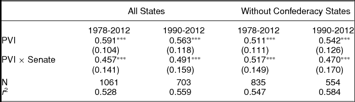
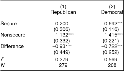




Comments
No Comments have been published for this article.