INTRODUCTION
As the science of climate change increasingly gains acceptance across the world communities, researchers and the general public are questioning how seriously such changes could harm the planet, where the most damage would occur and how societies should respond to the challenges (Solomon et al. Reference Solomon, Qin, Manning, Marquis, Averyt, Tignor, Miller and Chen2007; Nordhaus Reference Nordhaus2008). It is widely believed that low-latitude developing countries, particularly Africa, will bear the brunt of the damage from global warming, despite moderate gains in some areas, because they depend heavily on agriculture, are already located in hot zones and have less capacity to adapt (Reilly et al. Reference Reilly, Baethgen, Chege, van de Geijn, Erda, Iglesias, Kenny, Patterson, Rogasik, Rotter, Rosenzweig, Sombroek, Westbrook, Bachelet, Brklacich, Dammgen, Howden, Joyce, Lingren, Schimmelpfennig, Singh, Sirotenko, Wheaton, Watson, Zinyowera, Moss and Dokken1996; Mendelsohn et al. Reference Mendelsohn, Dinar and Williams2006; Parry et al. Reference Parry, Canziani, Palutikof, Van Der Linden and Hanson2007). These countries should adapt to climate change by altering current farm practices in order to minimize the damage on agriculture (Reilly et al. Reference Reilly, Baethgen, Chege, van de Geijn, Erda, Iglesias, Kenny, Patterson, Rogasik, Rotter, Rosenzweig, Sombroek, Westbrook, Bachelet, Brklacich, Dammgen, Howden, Joyce, Lingren, Schimmelpfennig, Singh, Sirotenko, Wheaton, Watson, Zinyowera, Moss and Dokken1996; Adams et al. Reference Adams, Mccarl, Segerson, Rosenzweig, Bryant, Dixon, Connor, Evenson, Ojima, Mendelsohn and Neumann1999; Gitay et al. Reference Gitay, Brown, Easterling, Jallow, McCarthy, Canziani, Leary, Dokken and White2001; Smit & Pilifosova Reference Smit, Pilifosova, McCarthy, Canziani, Leary, Dokken and White2001; Smith & Olesen Reference Smith and Olesen2010). Recent research indicates that African farmers have coped with different climate conditions by deliberately managing animal husbandry (Boko et al. Reference Boko, Niang, Nyong, Vogel, Githeko, Medany, Osman-Elasha, Tabo, Yanda, Parry, Canziani, Palutikof, van der Linden and Hanson2007). When the climate is hotter and drier, they favour integrated farming, which includes both crops and livestock, over specialized crop farming (Seo Reference Seo2010). They also prefer to keep goats and sheep in hot zones and avoid beef cattle (Seo & Mendelsohn Reference Seo and Mendelsohn2008). In semi-arid and dry savannahs, farmers adopt sheep, whereas goats are farmed most often in lowland humid zones (Seo et al. Reference Seo, Mendelsohn, Dinar, Hassan and Kurukulasuriya2009). These findings can be critical not only because researchers have so far concentrated on the vulnerabilities of important crops while neglecting the livestock component of agriculture (Antle et al. Reference Antle, Capalbo, Elliott and Paustian2004; Parry et al. Reference Parry, Rosenzweig, Iglesias, Livermore and Fischer2004; Schlenker & Roberts Reference Schlenker and Roberts2009), but also because integrated farming and livestock management can serve as a principal adaptation measure for the farmers in Africa where crop productivities have remained low, even after decades of development efforts (Byerlee & Eicher Reference Byerlee and Eicher1997; World Bank 2008; Eitzinger et al. Reference Eitzinger, Orlandini, Stefanski and Naylor2010). Animal scientists report potentially serious effects of climate change on animal performance such as liveweight growth, milk production and reproduction, or indirect effects through changes to grasslands, disease outbreaks and ecosystems, which may signal a large shift in agricultural systems in Africa due to climate change (Hahn Reference Hahn1999; Gitay et al. Reference Gitay, Brown, Easterling, Jallow, McCarthy, Canziani, Leary, Dokken and White2001; Mader Reference Mader2003; Butt et al. Reference Butt, Mccarl, Angerer, Dyke and Stuth2005; Polley et al. Reference Polley, Morgan and Fay2011).
Given this background, the present paper aims to develop further these past findings on adaptation to climate change by agricultural systems, to provide ‘ground level’ knowledge of adaptation strategies both to concerned farmers and policy makers by rescaling them to the Agro-Ecological Zones (AEZs) in Africa. The present paper makes the following three contributions to the existing literature: first, it utilizes the newly constructed spatial dataset of the World Bank, the Africa Infrastructure Country Diagnostic (AICD, World Bank 2009), to test the importance of market access variables such as travel times to a nearest city or to a major port. Secondly, the paper tests whether neighbourhood effects are dominant in the adoption of agricultural systems (Anselin Reference Anselin1988; Case Reference Case1992; Cressie Reference Cressie1993; Beron & Vijverberg Reference Beron, Vijverberg, Anselin, , Florax and Rey2004). A spatial bootstrapping model that could test and remove spatial correlations in the choices of neighbouring farms is developed. Thirdly, the major contribution of the present paper is, however, to provide a geographically scaled analysis of adaptation to climate change using adoption of agricultural systems. The aim is to explain the adoption of crops-only, livestock-only and integrated farming systems across the AEZs in Africa using the Food and Agriculture Organization's classification (FAO 2005). The key findings provided are differential measures of adaptation calibrated for each AEZ in Africa (Seo et al. Reference Seo, Mendelsohn, Dinar, Hassan and Kurukulasuriya2009).
The paper proceeds as follows: a spatial bootstrap logit model is developed, which tests and removes neighbourhood effects before estimating the choice of agricultural systems. Then farm surveys, climate, soils and other spatial information of Africa, compiled from various sources, are described. Finally, multinomial logit models are estimated with and without explicit spatial modelling. Based on the estimated parameters, simulations of adaptation behaviours by 2060 are made using a range of climate scenarios. The paper concludes with discussions on policy implications and overall assessments of the results.
MATERIALS AND METHODS
Animal husbandry is an essential component of farming in Africa. Many of the farms, c. 0·66, have both crops and livestock as their assets. It is rare for African farms to specialize in livestock, although there are some. Scientists reported that livestock productivities such as liveweight gain, milk production, wool production and reproduction are climate sensitive (Johnson Reference Johnson1965; Hahn Reference Hahn1999; Mader Reference Mader2003). Climate change is reported to affect the availability of livestock feed such as pastures and grains (Reilly et al. Reference Reilly, Baethgen, Chege, van de Geijn, Erda, Iglesias, Kenny, Patterson, Rogasik, Rotter, Rosenzweig, Sombroek, Westbrook, Bachelet, Brklacich, Dammgen, Howden, Joyce, Lingren, Schimmelpfennig, Singh, Sirotenko, Wheaton, Watson, Zinyowera, Moss and Dokken1996; Adams et al. Reference Adams, Mccarl, Segerson, Rosenzweig, Bryant, Dixon, Connor, Evenson, Ojima, Mendelsohn and Neumann1999; Sankaran et al. Reference Sankaran, Hanan, Scholes, Ratnam, Augustine, Cade, Gignoux, Higgins, Le Roux, Ludwig, Ardo, Banyikwa, Bronn, Bucini, Caylor, Coughenour, Diouf, Ekaya, Feral, February, Frost, Hiernaux, Hrabar, Metzger, Prins, Ringrose, Sea, Tews, Worden and Zambatis2005; Polley et al. Reference Polley, Morgan and Fay2011). Recent studies have found that African farmers adapt to climate change by selecting livestock species and agricultural systems given the current climate conditions (Seo & Mendelsohn Reference Seo and Mendelsohn2008; Seo Reference Seo2010). As geographic factors (defined below) and climate conditions vary across Africa, farm practices diverge widely throughout the continent.
In order to elaborate further the choice of agricultural systems across AEZs in Africa, a traditional multinomial logit model based on the motive of profit maximization was employed, which is broadly defined to be inclusive of household consumptions and family labours in the context of Africa. A farmer chooses the agricultural system j (where j=1, 2,…, J) that gives the highest profit given the climate. In the present analysis, three agricultural systems are analysed: a specialized crop system, a specialized livestock system and integrated farming. Systems were classified according to the direct answer given by farmers to the survey question: ‘Do you own livestock?’ A farm is defined to manage crops if there is any harvest recorded of any crops, regardless of sale or consumption in the household.
Let the profit from farm type j for household n be written as the sum of the observable component (V) and the error term (ε) as follows:

where j is a categorical variable which indicates J alternatives. The vector Z represents the set of explanatory variables that determine the net revenue of the farm. It includes geographic factors in detail in the present analysis, particularly travel time to a major port, travel time to a nearest city, soil textures and farm altitude, in addition to the factors such as climate, soils, water availability and household characteristics.
Assuming the error is independently and identically type I extreme value distributed and the function V can be written linearly in the parameters, the probability that the farmer will choose system j among the J available systems can be written succinctly as follows, after successive integrations of the probability density functions (McFadden Reference Mcfadden and Zarembka1974):

The parameters in the above equation (γ j) are estimated by the maximum likelihood method using an iterative non-linear optimization technique, the Newton–Raphson method. These estimates are consistent and asymptotically normally (CAN) distributed under regularity conditions.
To test neighbourhood effects, the means of the variance of the difference in the net revenues at two locations are defined. Let s denotes a specific location and h a directional distance from a specific location and define the following variance (Cressie Reference Cressie1993):

Measuring this variance across all the data points yields 1/2×n×(n–1) measures of Eqn (3) with n farms in the survey. If there is spatial continuity, then as h becomes larger, so will the difference in the values of Z between two locations and the variance of the difference of the net revenues. In other words, net revenues of the farms within a district are closer to each other than those of the farms within a larger geographical area, e.g. a country where there is spatial continuity.
The hypothesis is that the variance in Eqn (3) will reveal a great deal of spatial correlation of net revenues and choices, which will be discussed in detail in the ensuing empirical section. To remove this correlation or neighbourhood effects, the following spatial sampling and bootstrapping can be conducted. First, the whole sample is divided into subsets of districts. Secondly, one data point within each district is randomly selected, for all the districts with the data set. Thirdly, the results are bootstrapped by repeating this spatial sampling 300 times. Then, the spatially bootstrapped estimates of climate sensitivity parameters are defined as follows (Efron Reference Efron1979; Efron & Tibshirani Reference Efron and Tibshirani1994):

The notations are defined as follows: γ is the climate sensitivity parameter, j the agricultural systems, k the number of independent variables, S the spatial samples, R the number of bootstrap repetitions, B the bootstrapped parameters and T for the transpose of the matrix.
Then, the spatially bootstrapped probabilities are calculated as the means of the probabilities from the bootstrapped samples:

The uncertainties around the parameters are defined as confidence intervals at P>0·95 of the bootstrapped parameter estimates. These spatially bootstrapped probabilities are consistent and efficient as any other bootstrapped statistics.
The impacts of climate change on the choice of farm n are measured as follows. Let C a and C b be two states of climate, after and before climate change. Then, the change in the choice of agricultural system j is measured as the following difference in probabilities:

Adoption probabilities of agricultural systems would differ by the underlying climate and geographic conditions. If n k∈AEZκ and climate is to change from C kb to C ka in this zone, then the expected change is calculated as

The method was applied to an African data set, constructed with data obtained from various sources. Household variables, including choice decisions and farm characteristics, are based on the GEF/World Bank household surveys of African farms (Dinar et al. Reference Dinar, Hassan, Mendelsohn and Benhin2008). The surveys asked farmers detailed questions on crops and livestock management activities during the farming period from July 2002 to June 2003 for the following ten countries: Niger, Burkina Faso, Senegal and Ghana from West Africa, Cameroon from Central Africa, Kenya and Ethiopia from East Africa, South Africa and Zambia from Southern Africa and Egypt from North Africa. These countries cover all the sub-regions and all the 16 AEZs of Africa. A total of 9597 surveys were administered across the ten countries in the study. Surveys were collected randomly from the districts that are selected which cover diversity of climate conditions in each country.
Climate data are from the satellites operated by the US Department of Defence (the Special Sensor Microwave/Imager (SSMI)) and also from the ground weather stations across Africa. The satellites have measured surface temperatures at the centroid of each district around the globe from 1988 to the present time (Basist et al. Reference Basist, Grody, Peterson and Williams1998). Precipitation data came from the Africa Rainfall and Temperature Evaluation System (ARTES) (World Bank 2003). This data set, created by the (USA) National Oceanic and Atmospheric Association's Climate Prediction Center, is based on ground station measurements of precipitation in Africa.
Soil data were obtained from the FAO's Digital Soil Map of the World CD-ROM (FAO 2003). It provides information about the major and minor soils as well as slope and texture across the world. Hydrology data came from the University of Colorado's hydrology model, which measured water flow and runoff for each district in Africa (Strzepek & McCluskey Reference Strzepek and Mccluskey2006).
Spatial variables were obtained from the recently constructed World Bank spatial dataset. The present study uses travel times to the nearest city and to a major port computed by the World Bank project on Africa Infrastructure Country Diagnostic (World Bank 2009). Elevation at the centroid of each district was provided by the United States Geological Survey (USGS 2004).
RESULTS
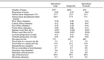
Descriptive statistics of the variables used in the present study are summarized in Table 1 for each of the three agricultural systems. More than half of the farms are integrated farms owning both crops and livestock. Only a small fraction of the sample, about 0·05, specializes in livestock. Almost 0·40 of the farms specialize in crops. Livestock-only and integrated farms are located, on average, in a hotter temperature zone but a lower precipitation zone. Geographic factors vary across agricultural systems. Integrated farms are more often located in West Africa. Specialized farms are located nearer to a city or to a major port than integrated farms, probably due to easy access to markets. Specialized crop farms are located at higher elevations. Where water flow is higher, it tends to be associated with specialized farms rather than integrated farms. Differences can be seen in household characteristics across different farm types. The farms that have some livestock have a larger number of family members; household labour, often involving the women and/or children, can be used to manage livestock grazing. When the property is owned by the farmer, it is more likely to be a specialized livestock farm. Extension service is mainly directed towards a specialized crop system and is rare in livestock systems. Some variables do not seem to diverge greatly. For example, farmers are educated for about 4·6 years and aged 48 years, regardless of agricultural systems adopted.
Means of variables by agricultural systems

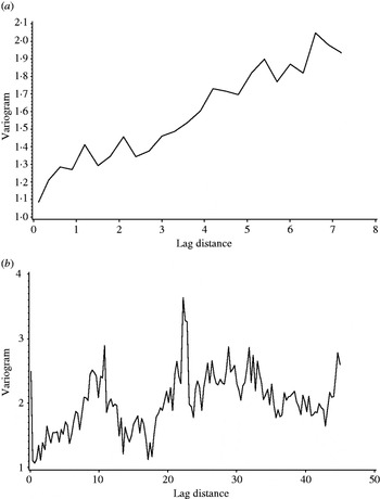
The means of the variance (Eqn (3)), explained in the theory section (Cressie Reference Cressie1993), was used to test whether substantial neighbourhood effects exist in the adoption of agricultural systems. In Fig. 1, two variograms of the log of net revenues/ha of land of the whole sample and the spatially selected samples are presented. The variogram plots the means of the variance in Eqn (3) over 20 subsets of equal distance between points. The whole sample variogram reveals that the variance increases as the distance between data points increases. It shows a linearly increasing trend over distance. This indicates that closer farms have more similar net revenues, indicating spatial correlation.
Variograms of (a) the whole sample v. (b) the spatially bootstrapped sample.

To account for neighbourhood effects, a spatial sampling explained in the theory section was conducted repeatedly, 250 times. The baseline geographical unit for spatial random sampling was districts, the second administrative division in the sample. The first bootstrap sample was then used to draw the same variogram. The figure in the bottom of Fig. 1 indicates that the spatial sampling essentially removed the spatial continuity in the top figure, i.e. a linearly increasing trend. The variogram fluctuates without any increasing trend. Therefore, the first step of a ‘spatial bootstrap’ approach was successful. The results were robust to sample selection and distance choice used for the variogram plot.
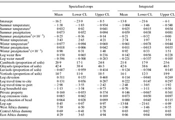
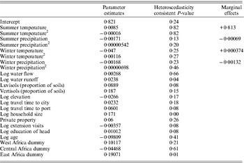
The second step was to conduct a multinomial logit analysis of the spatially selected sample. Spatial sampling was done by sampling only one observation farm from the cluster of farms in the neighbourhood, i.e. the district. The spatially selected sample had 377 observations and 250 samples of the equal size are randomly created. Table 2 summarizes bootstrapped means of parameter estimates along with their bootstrapped confidence intervals at P>0·95 from the 250 estimates of the corresponding parameters. Three spatial variables were entered and found to be significant factors: elevation, distance to a major port and distance to the nearest city. When travel time to the nearest city increases, integrated farming and a specialized crop system are more likely to be chosen, i.e. have higher log-odds, than a specialized livestock system. That is, specialized livestock farms are more likely to be located near a city. When travel time to a major port increases, however, both integrated farming and a specialized crop system are less likely to be chosen. These spatial patterns reflect the fact that Africa exports crops to the rest of the world and meat consumption is concentrated in the major cities. Farms in high altitudes are more likely to be crops-only.

The estimates of climate parameters are mostly significant except for winter precipitation. Where water flow is high, a farm is more likely to have crops as opposed to specializing in livestock. When runoff is high, the farm is more likely to be a specialized livestock system, due primarily to the soil conditions of these areas where forests are sparse or in steep slopes. A specialized crop system is less often chosen when the underlying soil is Luvisols which are found in the desert zones in southern and eastern Africa (FAO 2003). Integrated farming is chosen widely across Cambisols, Gleysols and Vertisols.
Household characteristics were controlled in detail by using household education, extension visits, age of the head, household size and land ownership. Knowledge and experience variables are regarded as important in improving farm productivity (Evenson & Gollin Reference Evenson and Gollin2003; Schultz Reference Schultz2004; Deressa et al. Reference Deressa, Hassan and Ringler2010). Farms with more extension visits tend to be crop-only over livestock-only. It could be that extension service is provided more often for crops rather than livestock in Africa, due to extensive development efforts directed towards major crops such as maize (Byerlee & Eicher Reference Byerlee and Eicher1997). More educated farm heads are more likely to avoid specialization in livestock. Older farm heads choose integrated farming less often. A larger family is more likely to specialize in livestock.
Focusing on sub-Saharan Africa, regional fixed effects were assessed by regional dummy variables for West Africa, East Africa, Central Africa, after setting South Africa as the base case. In particular, the West African dummy was expected to account for the more frequent outbreaks of livestock diseases and higher weather-related risks in the region (Ford & Katondo Reference Ford and Katondo1977; Hulme et al. Reference Hulme, Doherty, Ngara, New and Lister2001). The estimated parameters show that farmers in West Africa and East Africa preferred crops-only more than South African farmers. Integrated farming is more likely to be chosen in Central and East Africa and less likely in West Africa than in South Africa. This may reflect the fact that the specialized livestock operation is mainly located in South Africa. Regional dummies may also capture region specific policy distortions or trade agreements (Anderson & Masters Reference Anderson and Masters2009).
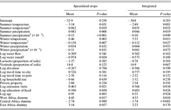
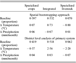
Since climate and soils in the present paper are calibrated at the district level, an additional analysis of a primary agricultural system at the district level is provided in Table 3. Based on the individual household's choice of agricultural systems, the system chosen most often is defined as the primary system in each district and a logit analysis of choice is conducted using the same set of independent variables. As shown in the table, the climate variables are again highly significant along with other soil and socio-economic variables.

In Table 4, marginal effects of climate variables based on the parameter estimates in Tables 2 and 3 are measured. It shows that a temperature increase of 1°C would increase the adoption of integrated farming by 0·7%. An increase in rainfall of 1% would decrease integrated farming by 0·07% while it would increase crops-only by a similar magnitude. This may be because more abundant rainfall shifts the ecosystem from grasslands to forests (Sankaran et al. Reference Sankaran, Hanan, Scholes, Ratnam, Augustine, Cade, Gignoux, Higgins, Le Roux, Ludwig, Ardo, Banyikwa, Bronn, Bucini, Caylor, Coughenour, Diouf, Ekaya, Feral, February, Frost, Hiernaux, Hrabar, Metzger, Prins, Ringrose, Sea, Tews, Worden and Zambatis2005; Polley et al. Reference Polley, Morgan and Fay2011) or prevalence of livestock diseases under such condition (Ford & Katondo Reference Ford and Katondo1977; University of Georgia 2007). In addition, the results indicate that a slightly higher temperature would decrease the choice of specialized livestock farming by 0·8%.
Marginal effects (%) on the choice probabilities of agricultural systems

When the parameters from the district level analysis in Table 3 are used, the increase in integrated farming is more than triples to +2·6% in response to a marginal increase in temperature. This increase is offset mostly by a loss in the specialized livestock system. When rainfall increases marginally, the specialized crop system increases, whereas the specialized livestock system decreases by c. 0·05%, respectively.
To test further the sensitivity of the results, the regression of the fraction of integrated farming in each district was run against the same set of explanatory variables, shown in Appendix 1. Based on the estimated parameters, the marginal effects of temperature and precipitation on the fraction of integrated farming in districts were also calculated. The results confirm the previous two analyses. That is, a marginal increase in temperature is expected to increase the proportion of integrated farming by >80%, whereas a marginal increase in precipitation to decrease this fraction only slightly.
The key component of the present analysis is concerned with practical adaptation information, i.e. how farmers should choose a specific system across different AEZs in Africa and how their choices should be adjusted when the current climate is to be altered. The importance of this additional task can be best understood in terms of the design of an efficient adaptation strategy. As agro-ecological condition varies on the ground, adaptation measures should be adopted in a mosaic pattern and avoid a blanket approach applied uniformly across Africa (Seo et al. Reference Seo, Mendelsohn, Dinar, Hassan and Kurukulasuriya2009). For this purpose, the AEZ classification of Africa into the 16 zones by the FAO (FAO 2005; Seo et al. Reference Seo, Mendelsohn, Dinar, Hassan and Kurukulasuriya2009) was used. Africa is classified into six agro-ecosystem types depending upon the length of crop growing season: desert, semi-arid, dry savannah, moist savannah, sub-humid and humid forest. Excluding the desert zone, each of the five zones is further divided into lowland, mid-elevation and high elevation. Desert zones are located in the Sahara and the south-western edge of the continent. South of the Sahara desert is a semi-arid zone, followed by dry savannah, moist savannah and humid forest in sequence. In central Africa around Cameroon, it is mostly humid forest in lowland. This low-elevation humid forest turns into mid-elevation and then into dry savannah as it stretches east towards Kenya. South of the humid forest is moist savannah, followed by dry savannah. The AEZs of South Africa are mostly moist savannah in the east, dry savannah in the centre and desert in the west. The highlands are located around Mount Kilimanjaro.
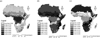
Figure 2 shows the present distributions of the three agricultural systems across the AEZs. The contrast between crops-only and integrated farming is evident. The crops-only farming is adopted most frequently in the lowland humid forest, lowland sub-humid and mid-elevation sub-humid AEZs. Rate of adoption is also high in the highlands in the East and in South Africa. On the other hand, integrated farming is favoured in the dry zones of West Africa. The lowland dry savannah, semi-arid and desert zones have the highest likelihood to choose integrated farming. This system is also chosen most often in the eastern coast lowland arid zones. However, integrated farming is quite common in dry places in mid-elevations.
Current probabilities of selecting (a) specialized crops, (b) integrated farming and (c) specialized livestock.

The contrasts between a specialized crop system and a specialized livestock system are also evident. Overall, the likelihood of the specialized livestock system is much lower across Africa. While a specialized crop system is found most often in Central Africa, a specialized livestock system is most often adopted in South Africa and North Africa. Livestock-only farms are most common on the mid-elevation moist and dry savannah zones in Southern Africa.
A geographically scaled adaptation to climate scenarios
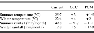
Extending the marginal analyses, the impacts of climate change on agricultural systems based on multiple climate prediction models were simulated. A set of climate scenarios from the Atmospheric Oceanic General Circulation Models (AOGCMs) were used to cover a broad range of estimates that are consistent with the estimates in the most recent Intergovernmental Panel on Climate Change (IPCC) report (Solomon et al. Reference Solomon, Qin, Manning, Marquis, Averyt, Tignor, Miller and Chen2007). Specifically, simulation results are presented from the following two models, as their predictions are quite different: CCC (Canadian Climate Centre, Boer et al. Reference Boer, Flato and Ramsden2000) and PCM (Parallel Climate Model, Washington et al. Reference Washington, Weatherly, Meehl, Semtner, Bettge, Craig, Strand, Arblaster, Wayland, James and Zhang2000). The scenarios correspond to the A2 emission scenarios from the Special Report on Emissions Scenarios (SRES) of the IPCC (IPCC 2000). Table 5 summarizes the seasonal mean temperatures and precipitations projected by the two models for the year 2060. The PCM scenario predicts a 1·7°C increase and CCC a 3·5°C increase in annual mean temperature. The PCM predicts a 5% increase in annual mean rainfall in Africa, but the CCC, a 10% decrease by 2060. There is also a substantial variation in rainfall across countries within each scenario.
AOGCM climate scenarios for 2060

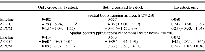
Based on the parameter estimates in Table 2 and the AOGCM scenarios in Table 5, adaptive responses under each scenario are calculated for each agricultural system in Table 6. The estimates are means and confidence intervals at P>0·95 estimated from 250 bootstrapping runs of the spatially selected samples. It reconfirms that integrated farming would increase under the CCC scenario by 4%. In addition, it confirms that crops-only would increase under the PCM scenario, albeit slightly. It predicts the livestock-only system would increase slightly under the hot and dry CCC scenario. Finally, integrated system increases only when there is a higher temperature increase and a substantial reduction in rainfall under the CCC scenario, but not in the PCM scenario. However, the increase in the crops-only under the PCM scenario, the increase of the livestock-only under the CCC scenario, and the decrease of integrated farming under the PCM scenario are not significant at P<0·05 according to the bootstrap confidence intervals.
Changes of the choice probabilities (%) of agricultural systems by AOGCM scenarios

* The numbers in parentheses are bootstrapped confidence intervals at P>0·95.
A sensitivity analysis of the inclusion of seasonal water flows in m3/s in each district is provided in Table 6. When both summer water flow and winter water flow are included in the model, the predictions from the PCM scenario become noticeably different. It predicts much larger increase in the crop-only system and much larger decrease in the mixed system. The large magnitudes of changes are not reasonable since the expected climate change is moderate under the PCM scenario. They might be caused by a high correlation between summer water flow and winter water flow at the district level.
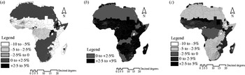
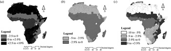
Finally, adaptive changes in the estimated probabilities of the three agricultural systems in 2060 under the two climate scenarios are mapped in Figs 3 and 4. Under the CCC scenario, as shown in Fig. 3, the crops-only system moves out from the currently favoured regions of sub-humid and humid forest regions in the lowlands. This system is reduced by >5% in the lowland savannahs located in West Africa and eastern coastal zones. It moves towards the mid- and high elevations and to the desert zones. The increase in the desert zone may capture that the surveys were drawn from the farms in the desert zones only when there is sufficient water suitable for crops. On the other hand, integrated farming increases across all the AEZs by >2·5%, but less so in the deserts or in the humid forest zones in the mid- or high elevations. A livestock only farming declines almost everywhere except in the lowland semi-arid, dry savannah and moist savannah zones in the lowlands by 2–5%.
Changes in probabilities of selecting (a) specialized crops, (b) integrated farming and (c) specialized livestock under the CCC scenario.

Changes in probabilities of selecting (a) specialized crops, (b) integrated farming and (c) specialized livestock under the PCM scenario.

Figure 4 shows adaptation maps under the PCM scenario. Under this mild scenario, crop-only farming increases in most places in mid- and high elevations. It increases in the currently arid zones owing to increased precipitation. However, in most lowland zones, this system declines. In the lowland semi-arid, dry savannah and moist savannah zones, farmers would adopt specialized livestock system more often. Integrated farming declines across Africa, but more heavily in the deserts.
DISCUSSION
The present paper provides a geographically scaled analysis of adaptation to climate change using the currently observed adoption of agricultural systems by African farmers located across varied climate zones. The recommendations, therefore, are limited to potential shifts of the three main farming systems defined herein. In addition, the micro-econometric approach taken in the present paper does not explain why a specific agricultural system dominates in a certain climate zone, but only relationships between the adoption of systems and climate, after controlling relevant soils, geography, water flows, household characteristics and regional dummies. Future adaptations tabled in the present paper are valid only if the overall regional production conditions should remain the same while the analytical framework itself allows researchers to measure the impacts of a change in covariates, e.g. more provision of electricity to sub-Saharan Africa or better extension service.
A policy implication of the results is clear: that integrated farming should be adopted more often in a hot and dry climate in the future, possibly because of diversification benefits under climate risks (Tobin Reference Tobin1958; Seo Reference Seo2010). This advice remains valid under the three different approaches taken in the present paper: a spatial bootstrap approach, a district dominant system approach and a fraction of integrated farming approach at the district level. In addition, the geographical scaling, either scaling up or scaling down, reveals that such adaptation measures should accommodate the agro-ecological conditions on the ground (Seo et al. Reference Seo, Mendelsohn, Dinar, Hassan and Kurukulasuriya2009). That is, crops-only should increase vastly in mid- and high elevations when climate turns out to be milder and wetter, while livestock-only should increase in lowland savannah zones under the CCC scenario. In addition, individual adaptations as well as public supports for them should take into account household characteristics such as age, gender, education and property ownership, as outlined in this paper in contrast to other approaches (Adams et al. Reference Adams, Mccarl, Segerson, Rosenzweig, Bryant, Dixon, Connor, Evenson, Ojima, Mendelsohn and Neumann1999; Butt et al. Reference Butt, Mccarl, Angerer, Dyke and Stuth2005).
Since Africa is highly dependent on agriculture, employing more than 0·80 of the population in sub-Saharan Africa, the findings are critically important for food security under climate stress (World Bank 2008). Understanding agricultural adaptations as merely switching to selected crops can be misleading without considering the decision to switch to livestock systems (Parry et al. Reference Parry, Rosenzweig, Iglesias, Livermore and Fischer2004; Schlenker & Roberts Reference Schlenker and Roberts2009). Similarly, the efforts to eliminate poverty in Africa may not be successful by focusing on selected crops such as maize, but must heed livestock production also (Byerlee & Eicher Reference Byerlee and Eicher1997).
Several qualifications of the results deserve to be mentioned. The present paper does not consider the effects of carbon doubling on crops or livestock, but only temperature and rainfall effects (Reilly et al. Reference Reilly, Baethgen, Chege, van de Geijn, Erda, Iglesias, Kenny, Patterson, Rogasik, Rotter, Rosenzweig, Sombroek, Westbrook, Bachelet, Brklacich, Dammgen, Howden, Joyce, Lingren, Schimmelpfennig, Singh, Sirotenko, Wheaton, Watson, Zinyowera, Moss and Dokken1996; Lobell & Field Reference Lobell and Field2008). If carbon doubling would benefit one or the other more seriously, it could tilt the choice of agricultural systems into one direction or the other. In addition, the present paper assumes that adaptive changes take place as needed by individuals (Cline Reference Cline1996; Kelly et al. Reference Kelly, Kolstad and Mitchell2005). Whether some sub-regions or individuals would find it difficult to change to a certain agricultural system is not considered by the present paper. However, the cost of making this transition is not expected to be high for most farms, since it belongs to a common farm operation and can be most likely to be captured in the shifts in long-run equilibriums.
I would like to thank the World Bank for supporting the Climate Change and Agriculture Project in Africa from which the survey data are constructed. I am particularly grateful to Robert Mendelsohn, Ariel Dinar, Rashid Hassan and Pradeep Kurukulasuriya. The spatial data are obtained from the World Bank spatial data team with the help of Donald Larson to whom I would like to express my gratitude. The paper has benefited from the comments of the anonymous reviewers of the Journal to whom I owe appreciation. The views expressed in this paper are the present author's alone.