


INTRODUCTION
According to Yuhua Wang’s (Reference Wang2022) “Blood is Thicker Than Water: Elite Kinship Networks and State Building in Imperial China” (hereafter BITTW) in American Political Science Review, geographically dispersed kinship networks incentivize political elites to support the building of a strong state, whereas geographically concentrated kinship networks undermine state building. Using as case study elite responses to Wang Anshi’s Reform (hereafter “Reform” for short)—an ambitious and controversial package of dozens of policies intended to strengthen state capacity—during the reign of Northern Song Emperor Shenzong (1067–1085 CE), BITTW collected a novel set of data by scraping kinship information from all available tomb epitaphs of Shenzong-era politicians and identifying their wives, sons, daughters and children-in-law manually. It then tabulated each politician’s degree of local concentration of kin (hereafter LCK) and measured its correlation with his attitude toward Reform.
Despite BITTW’s creative and industrious procurement of information, it—like most research in quantitative history—faced a severe “missing data” problem from the outset, due to the inevitable incompleteness of historical records. This problem is exacerbated by BITTW’s inadequate engagement with Chinese historical scholarship on the Reform’s partisanship geography, giving rise to flaws in its coding and theorizing. In this article, I first mitigate the missing-data problem by procuring additional information from relevant historical records, thereby increasing the sample size by half. As it turns out, BITTW’s key finding fails to replicate with the improved sample when either the control issue or the outlier issue is considered. I then propose two alternative hypotheses on the role of kinship network dispersal in Reform, based on two common explanations of its partisanship geography in Chinese historical scholarship, that is, status competition and policy adaptiveness. After examining those hypotheses respectively, I reflect on the limits of quantitative history this case illustrates.
IMPROVING THE SAMPLE
Data Lost and Found
Among the 137 politicians included in its robustness checks, BITTW only obtained full information on all the variables for 40 politicians, on whom it conducted the main analysis. To assuage worries over the meaningfulness of statistical findings with such a small sample, BITTW meticulously applied all the standard confidence-enhancing procedures in quantitative social science, for which it deserved recognition. Nonetheless, being measures of last resort, those procedures are themselves no substitute for a higher-quality sample.
In fact, there is room to improve the sample. Among those excluded from BITTW’s main analysis, there are 28 whose kinship information was procured but whose partisanship information was left blank (Wang Reference Wang2022, Dataset). By taking a closer look at historical records, however, we can retrieve information on the partisan stances of at least 21 politicians among those 28, increasing the sample size from 40 to 61 for the main analysis.Footnote 1 In particular, most of the information exists in the two major documents BITTW relied on, namely, Xu Zizhitongjian Changbian (The Extended Continuation to Comprehensive Mirror in Aid of Governance, compiled in the twelfth century) (Li Reference Li1995) and Song Shi (The History of Song, compiled in the fourteenth century) (Toghtō 1975). Supplementary as well as corroborative information can be retrieved from other historical materials, such as Sushui Jiwen (Records of Rumors by the River of Su, personal notes Wang Anshi’s nemesis Sima Guang left behind) (Sima Reference Sima1936).
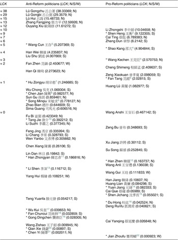
Table 1 presents the expanded list of 26 pro-Reform and 35 anti-Reform politicians for the main analysis, in descending order of LCK. It also groups them in terms of their rounded LCK values, so as to give readers a more intuitive sense of the sample’s configuration. The politicians on whom BITTW did not procure partisanship information are marked with asterisks, and their relevant historical records are provided in the respective footnotes. For the sake of simplicity, hereafter I call BITTW’s original sample for the main analysis the O-Sample, and my expanded sample the E-Sample. Meanwhile, for reasons to be explained later, I also include every politician’s hometown region information in Table 1, coded as “N” if one came from north of “the Huai River, the Tongbai Mountain, the midstream Han River and the Daba Maountains” (Yang Reference Yang1982, 165):Footnote 23 as “S” if one came from south of that line; and as “W” if one came from the then culturally and economically distinct Southwest, roughly equivalent to present-day Sichuan and Chongqing (Liu Reference Liu1959, 28–9).
Expanded List of Politicians for the Main Analysis, with Information on Hometown Region, in Descending Order of LCK
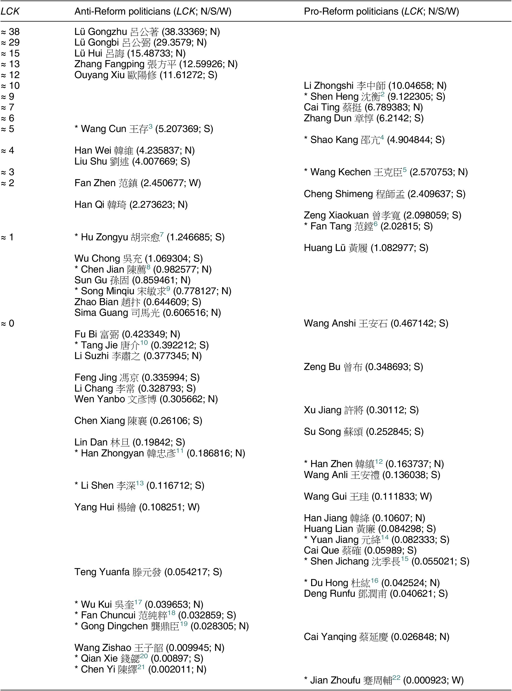
Table 1. Long description
The table consists of three columns: L C K, Anti-Reform politicians (L C K; N/S/W), and Pro-Reform politicians (L C K; N/S/W). Data is organized in descending order of L C K values.
* L C K approximately 38: Lü Gongzhu (38.33369; N) in the Anti-Reform column.
* L C K approximately 29: Lü Gongbi (29.3579; N) in the Anti-Reform column.
* L C K approximately 15: Lü Hui (15.48733; N) in the Anti-Reform column.
* L C K approximately 13: Zhang Fangping (12.59926; N) in the Anti-Reform column.
* L C K approximately 12: Ouyang Xiu (11.61272; S) in the Anti-Reform column.
* L C K approximately 10: Li Zhongshi (10.04658; N) in the Pro-Reform column.
* L C K approximately 9: Shen Heng (9.122305; S) in the Pro-Reform column.
* L C K approximately 7: Cai Ting (6.789383; N) in the Pro-Reform column.
* L C K approximately 6: Zhang Dun (6.2142; S) in the Pro-Reform column.
* L C K approximately 5: Wang Cun (5.207369; S) in Anti-Reform and Shao Kang (4.904844; S) in Pro-Reform.
* L C K approximately 4: Han Wei (4.235837; N) and Liu Shu (4.007669; S) in the Anti-Reform column.
* L C K approximately 3: Wang Kechen (2.570753; N) in the Pro-Reform column.
* L C K approximately 2: Anti-Reform includes Fan Zhen (2.450677; W) and Han Qi (2.273623; N). Pro-Reform includes Cheng Shimeng (2.409637; S), Zeng Xiaokuan (2.098059; S), and Fan Tang (2.02815; S).
* L C K approximately 1: Anti-Reform includes Hu Zongyu (1.246685; S), Wu Chong (1.069304; S), Chen Jian (0.982577; N), Sun Gu (0.859461; N), Song Minqiu (0.778127; N), Zhao Bian (0.644609; S), and Sima Guang (0.606516; N). Pro-Reform includes Huang Lü (1.082977; S).
* L C K approximately 0: This section contains the largest group. Pro-Reform includes Wang Anshi (0.467142; S), Zeng Bu (0.348693; S), Xu Jiang (0.30112; S), Su Song (0.252845; S), Han Zhen (0.163737; N), Wang Anli (0.136038; S), Wang Gui (0.111833; W), Han Jiang (0.10607; N), Huang Lian (0.084298; S), Yuan Jiang (0.082333; S), Cai Que (0.05989; S), Shen Jichang (0.055021; S), Du Hong (0.042524; N), Deng Runfu (0.040621; S), Cai Yanqing (0.026848; N), and Jian Zhoufu (0.000923; W). Anti-Reform includes Fu Bi (0.423349; N), Tang Jie (0.392212; S), Li Suzhi (0.377345; N), Feng Jing (0.335994; S), Li Chang (0.328793; S), Wen Yanbo (0.305662; N), Chen Xiang (0.26106; S), Lin Dan (0.19842; S), Han Zhongyan (0.186816; N), Li Shen (0.116712; S), Yang Hui (0.108251; W), Teng Yuanfa (0.054217; S), Wu Kui (0.039653; N), Fan Chuncui (0.032859; S), Gong Dingchen (0.028305; N), Wang Zishao (0.009945; N), Qian Xie (0.00897; S), and Chen Yi (0.002011; N).
Note: Politicians with * were omitted in BITTW’s main analysis; LCK: local concentration of kin (Wang Reference Wang2022, Dataset); N: North; S: South; W: Southwest
Notes on Coding
For its main analysis, BITTW adopted a “continuous” approach to coding a politician’s Support for Reform (hereafter SFR): namely, coding consistent support (i.e., across policies and over time) as 1; coding consistent opposition as 0; and coding a mixed attitude by way of the score “averaged across all policies” on which a politician’s view was specified in historical records (Wang Reference Wang2022, 904). As it turned out, BITTW only identified four mixed-attitude politicians in the O-Sample and one outside of it,Footnote 24 whereas all the other politicians were coded as either consistently anti-Reform or consistently pro-Reform. It is likely that BITTW considerably underestimated the prevalence of mixed attitudes; however, as there are quite a few other politicians well known for having either cross-policy mixed attitudes or temporally evolved attitudes toward Reform, both in the O-Sample (such as Wang Zishao)Footnote 25 as well as the rest of the E-Sample (such as Fan Chuncui and Wang Cun),Footnote 26 and among those whose kinship information BITTW did not procure (such as Su Shi and Zheng Xia).Footnote 27 In theory, a more thorough—and much more time-consuming—scraping of additional, rare historical sources (than what I have done to simply expand the sample for the main analysis) might provide us with a longer list of mixed-attitude politicians, each assigned a certain “averaged” SFR score greater than 0 and smaller than 1. But there is no point in doing so, for BITTW’s coding strategy of averaging across specified policies is fundamentally flawed and potentially misleading anyway.
To see why, take Li Chang for example. BITTW assigned him an SFR score of 0.166667, meaning that Li specifically opposed five Reform policies and supported one Reform policy according to available historical records. In reality, however, things were much more complicated. Li used to be Wang Anshi’s close friend and a strong supporter of Reform, and was hand-picked by Wang at the outset of Reform to be a deputy director of the newly established Steering Agency on Finances and Regulations (zhizhi sansi tiaoli si) in charge of devising and financing Reform policies. There, Li offered two pieces of advice to Wang: to slow down the pace of Reform, so as not to make too many enemies at once; and to drop certain ill-thought-out Reform policies from the package, such as the balanced delivery reform (junshufa) and the rural credit reform (qingmiaofa). Both pieces of advice infuriated Wang, however, who was infamously unable to take criticism. Shortly afterwards, Li was purged by Wang from the central government and appointed to various local and ceremonial positions over the next two decades. By the time Emperor Shenzong died, Li had become known as a vocal critic of Reform and was soon recruited by the anti-Reform party, which was incumbent through the Yuanyou Era (1086–1094 CE). Yet, he surprised and alienated his anti-Reform colleagues when they planned to abolish the “hired” labor service reform (muyifa) and restore the pre-Reform system of “assigned” labor service (chaiyifa). According to Li, the older system had been deserted for so long that there was no longer any reliable census data in place to support its implementation; instead, a mixed system should be strived for that would combine the strengths of muyifa and chaiyifa. Footnote 28
Li Chang’s case highlights two problems with BITTW’s coding strategy. First, its averaged SFR scores cannot capture a politician’s attitude change over time, be it toward Reform as a whole or toward any specific Reform policy. For example, we cannot tell from Li Chang’s SFR score (0.166667) that his overall attitude toward Reform changed from support to opposition. Similarly, we cannot tell from Wang Zishao’s SFR score (0) that his view on the rural credit reform changed from support to opposition.
Second, a politician’s SFR score averaged across the policies on which his view was specified in historical records could sometimes misrepresent his overall stance on Reform. After all, Reform was a package of dozens of policies, and a politician might, for a variety of reasons, only engage (or leave archival traces of engagement) in debates over a handful of those policies, even if he also had strong views on other policies or on Reform as a whole. For example, in accordance with BITTW’s coding strategy, Li Chang at the outset of Reform (i.e., excluding his later defense of the labor service reform during the Yuanyou Era, the only available historical record of him defending any specific Reform policy) would have gotten an SFR score of 0 (i.e., consistently anti-Reform), even though, as mentioned above, his criticisms of specific policies at the outset of Reform were made against the backdrop of his overall pro-Reform stance at the time. Similarly, BITTW gave Teng Yuanfa an SFR score of 0.5, leaving the impression that he was a moderate, even though he was actually a staunch opponent of Reform throughout.Footnote 29
I will return to these problems later, when discussing rival hypotheses to BITTW’s theory. For now, my point is that assigning a “continuous” SFR score to a mixed-attitude politician by way of averaging his expressed views on individual Reform policies, as BITTW did, is no better than simply assigning a “dichotomous” SFR score to him based on historical records about his overall attitude toward Reform (i.e., either anti-Reform or pro-Reform), at least when studying the effect of LCK on one’s attitude toward Reform. In other words, for the present purpose of replicating BITTW’s results with the E-Sample, it would be a waste of time either to code the additional 21 politicians “continuously” or to identify additional mixed-attitude politicians in the O-Sample for “continuous” coding. Rather, we should just assign dichotomous SFR scores (0 or 1) to all 61 politicians, including the four politicians coded “continuously” by BITTW.
REPLICATION
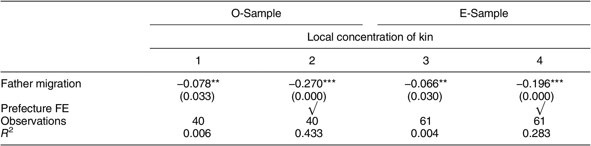
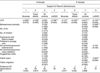
Replacing the O-Sample with the E-Sample, Table 2 replicates BITTW’s (Wang Reference Wang2022, Table 1) ordinary least squares (OLS) estimates of the correlation between a politician’s family migration patterns (Father migration) and the geographical span of his kinship networks (LCK), and Table 3 replicates BITTW’s (Wang Reference Wang2022, Table 2) OLS estimates of the correlation between the geographical span of a politician’s kinship networks (LCK) and his attitude toward Reform (SFR), which is now coded dichotomously rather than continuously. At first glance, both correlations remain significant in the E-Sample. However, there are two issues with the apparent LCK-SFR correlation.
OLS Estimates of the Correlation between Father Migration and Geography of Kinship Network (O-Sample vs. E-Sample)
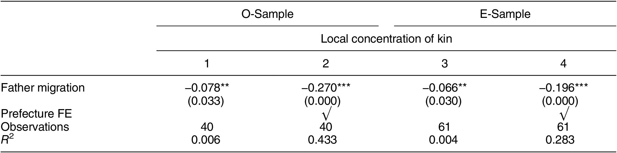
Table 2. Long description
The table presents O L S estimates across four columns. Columns 1 and 2 represent the O-Sample, while columns 3 and 4 represent the E-Sample. The dependent variable for all columns is the local concentration of kin.
* Father migration row:
- Column 1: minus 0.078 with two asterisks (standard error 0.033).
- Column 2: minus 0.270 with three asterisks (standard error 0.000).
- Column 3: minus 0.066 with two asterisks (standard error 0.030).
- Column 4: minus 0.196 with three asterisks (standard error 0.000).
* Prefecture F E row:
- Columns 2 and 4 contain a checkmark, indicating the inclusion of fixed effects, while columns 1 and 3 are blank.
* Observations row:
- O-Sample (columns 1 and 2): 40.
- E-Sample (columns 3 and 4): 61.
* R super 2 row:
- Column 1: 0.006.
- Column 2: 0.433.
- Column 3: 0.004.
- Column 4: 0.283.
Note: All variables are standardized. Three asterisks indicate p less than 0.01, and two asterisks indicate p less than 0.05.
Note: This table replicates BITTW’s estimates (Wang Reference Wang2022, Table 1) with both the O-Sample and the E-Sample. The dependent variable is an index of the local concentration of kin. The variable of interest is the distance between the politician’s father’s final residence and the politician’s grandfather’s hometown (Father migration). All variables are standardized. Robust standard errors clustered at the prefectural level are in parentheses. ***p < 0.01, **p < 0.05, *p < 0.10.
OLS Estimates of the Correlation between Geography of Kinship Network and Support for Reform (O-Sample vs. E-Sample)
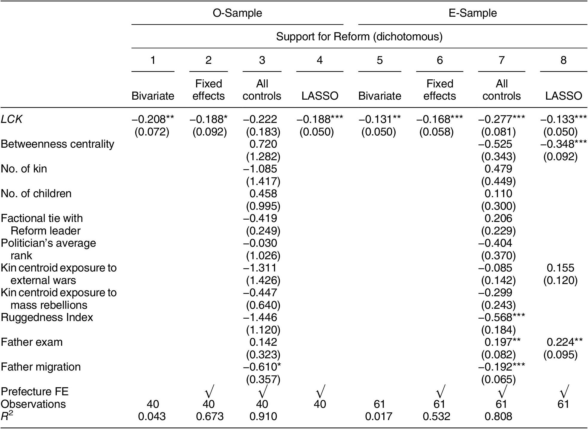
Table 3. Long description
The table presents regression results for two main groups: O-Sample (columns 1 to 4) and E-Sample (columns 5 to 8). The dependent variable is Support for Reform (dichotomous).
Key variables and their coefficients (standard errors in parentheses):
* L C K: Shows negative correlations across all models. In O-Sample, coefficients range from -0.188 to -0.222. In E-Sample, coefficients range from -0.131 to -0.277. Most are statistically significant at the 0.01, 0.05, or 0.10 levels.
* Betweenness centrality: 0.720 in O-Sample (column 3); -0.525 in E-Sample (column 7) and -0.348 in E-Sample (column 8).
* No. of kin: -1.085 (O-Sample) and 0.479 (E-Sample).
* No. of children: 0.458 (O-Sample) and 0.110 (E-Sample).
* Factional tie with Reform leader: -0.419 (O-Sample) and 0.206 (E-Sample).
* Politician’s average rank: -0.030 (O-Sample) and -0.404 (E-Sample).
* Kin centroid exposure to external wars: -1.311 (O-Sample) and -0.085 to 0.155 (E-Sample).
* Kin centroid exposure to mass rebellions: -0.447 (O-Sample) and -0.299 (E-Sample).
* Ruggedness Index: -1.446 (O-Sample) and -0.568 (E-Sample).
* Father exam: 0.142 (O-Sample) and 0.197 to 0.224 (E-Sample).
* Father migration: -0.610 (O-Sample) and -0.192 (E-Sample).
Model Specifications:
* Columns 1 and 5: Bivariate.
* Columns 2 and 6: Fixed effects (indicated by checkmarks for Prefecture F E).
* Columns 3 and 7: All controls.
* Columns 4 and 8: L A S S O.
Summary Statistics:
* Observations: 40 for O-Sample; 61 for E-Sample.
* R-squared: Ranges from 0.043 to 0.910 in O-Sample; 0.017 to 0.808 in E-Sample.
Note: This table replicates BITTW’s estimates (Wang Reference Wang2022, Table 2) with both the O-Sample and the E-Sample. The unit of analysis is an individual politician. The dependent variable is the politician’s Support for Reform, coded dichotomously. The variable of interest is an index of the local concentration of kin. All variables are standardized. Robust standard errors clustered at the prefectural level are in parentheses. ***p < 0.01, **p < 0.05, *p < 0.10.
The least absolute shrinkage and selection operator (LASSO) coefficients reported in columns 4 and 8 of this table (as well as in columns 4 and 8 of Tables 5 and 6, and in column 5 of Table 7) are based on the latest version of pdslasso (version 13, dated September 2024) provided by Achim Ahrens and Mark Schaffer on their github page https://github.com/statalasso/pdslasso/ for selecting the optimal choices of control variables. As it turns out, using the earlier “ssc” version of pdslasso they developed (version 1.3, dated July 2020), which was what Wang (Reference Wang2022) used, would yield different LASSO coefficients for Tables 3, 5, and 6, though not for Table 7. A possible explanation for those differences is that our sample sizes are just too small for LASSO regressions to be meaningful.
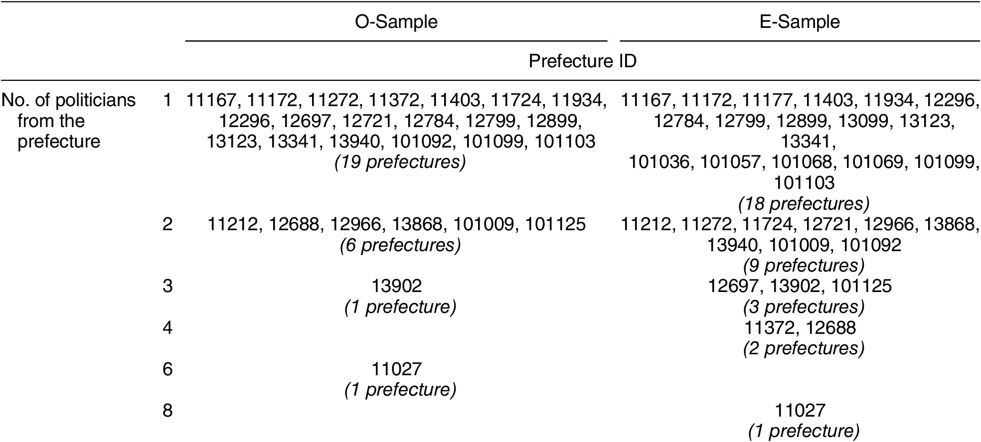
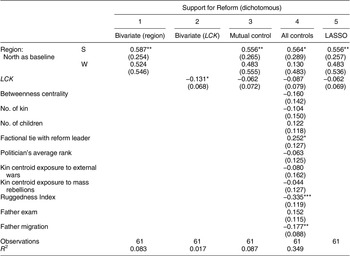
First, BITTW controlled for the fixed effects of a politician’s hometown prefecture while estimating the LCK-SFR correlation (Wang Reference Wang2022, 905–6). But as Table 4 shows, the distribution of politicians across prefectures, be it in the O-Sample or in the E-Sample, is so scattered that controlling for prefecture fixed effects might actually create a spurious correlation. By contrast, once we control for a politician’s hometown region, instead of hometown prefecture, the LCK-SFR correlation is no longer significant (see Table 7 below).
Distribution of Politicians across Prefectures (O-Sample vs. E-Sample)
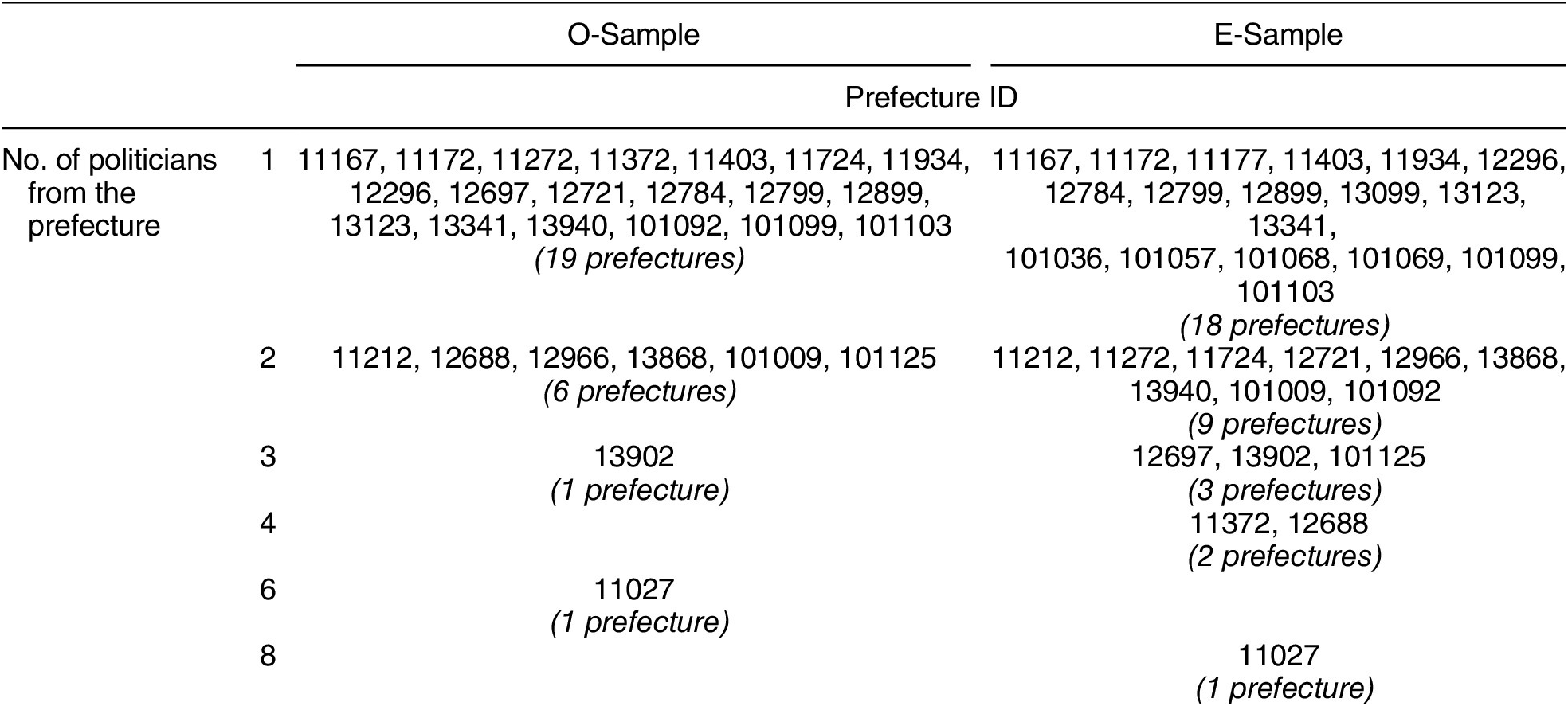
Table 4. Long description
The table is organized into four columns. The first two columns define the category: Number of politicians from the prefecture. The third column is the O-Sample and the fourth is the E-Sample. Both sample columns list specific Prefecture I D codes and the total count of prefectures in that category.
* For 1 politician: O-Sample has 19 prefectures (I D codes include 11167, 11172, 11272, 11372, 11403, 11724, 11934, 12296, 12697, 12721, 12784, 12799, 12899, 13123, 13341, 13940, 101092, 101099, 101103). E-Sample has 18 prefectures (I D codes include 11167, 11172, 11177, 11403, 11934, 12296, 12784, 12799, 12899, 13099, 13123, 13341, 101036, 101057, 101068, 101069, 101099, 101103).
* For 2 politicians: O-Sample has 6 prefectures (11212, 12688, 12966, 13868, 101009, 101125). E-Sample has 9 prefectures (11212, 11272, 11724, 12721, 12966, 13868, 13940, 101009, 101092).
* For 3 politicians: O-Sample has 1 prefecture (13902). E-Sample has 3 prefectures (12697, 13902, 101125).
* For 4 politicians: O-Sample is empty. E-Sample has 2 prefectures (11372, 12688).
* For 6 politicians: O-Sample has 1 prefecture (11027). E-Sample is empty.
* For 8 politicians: O-Sample is empty. E-Sample has 1 prefecture (11027).
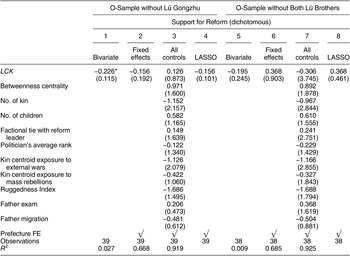
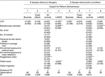
Second, most politicians in Table 1, anti-Reform and pro-Reform alike, have relatively low LCK scores, while only a small number of politicians have relatively high LCK scores. In particular, Lü Gongzhu (LCK = 38.33369) and Lü Gongbi (LCK = 29.3579), both anti-Reform, had exceptionally greater degrees of kinship concentration than everyone else—and, interestingly, they happened to be brothers (unrelated to Lü Hui, the politician with the third-highest LCK in Table 1). Could it be that the apparent LCK-SFR correlation, be it in the O-Sample or in the E-Sample, was due solely to the presence of either a single outlier individual (i.e., Lü Gongzhu) or a single outlier family (i.e., the two Lü brothers), even if we keep controlling for hometown prefecture instead of hometown region? Indeed, when we drop Lü Gongzhu alone from the O-Sample, the correlation is already on the verge of insignificance;Footnote 30 and if we drop the two Lü brothers as a cluster from the O-Sample, the correlation disappears (Table 5). Moreover, as soon as we drop Lü Gongzhu alone from the E-Sample, the correlation disappears as well (Table 6). In other words, replacing the O-Sample with the E-Sample demonstrates more forcefully the impacts of a single outlier individual on the reported results.
OLS Estimates of the Correlation between Geography of Kinship Network and Support for Reform (O-Sample Excluding either Lü Gongzhu or Both Lü Brothers)
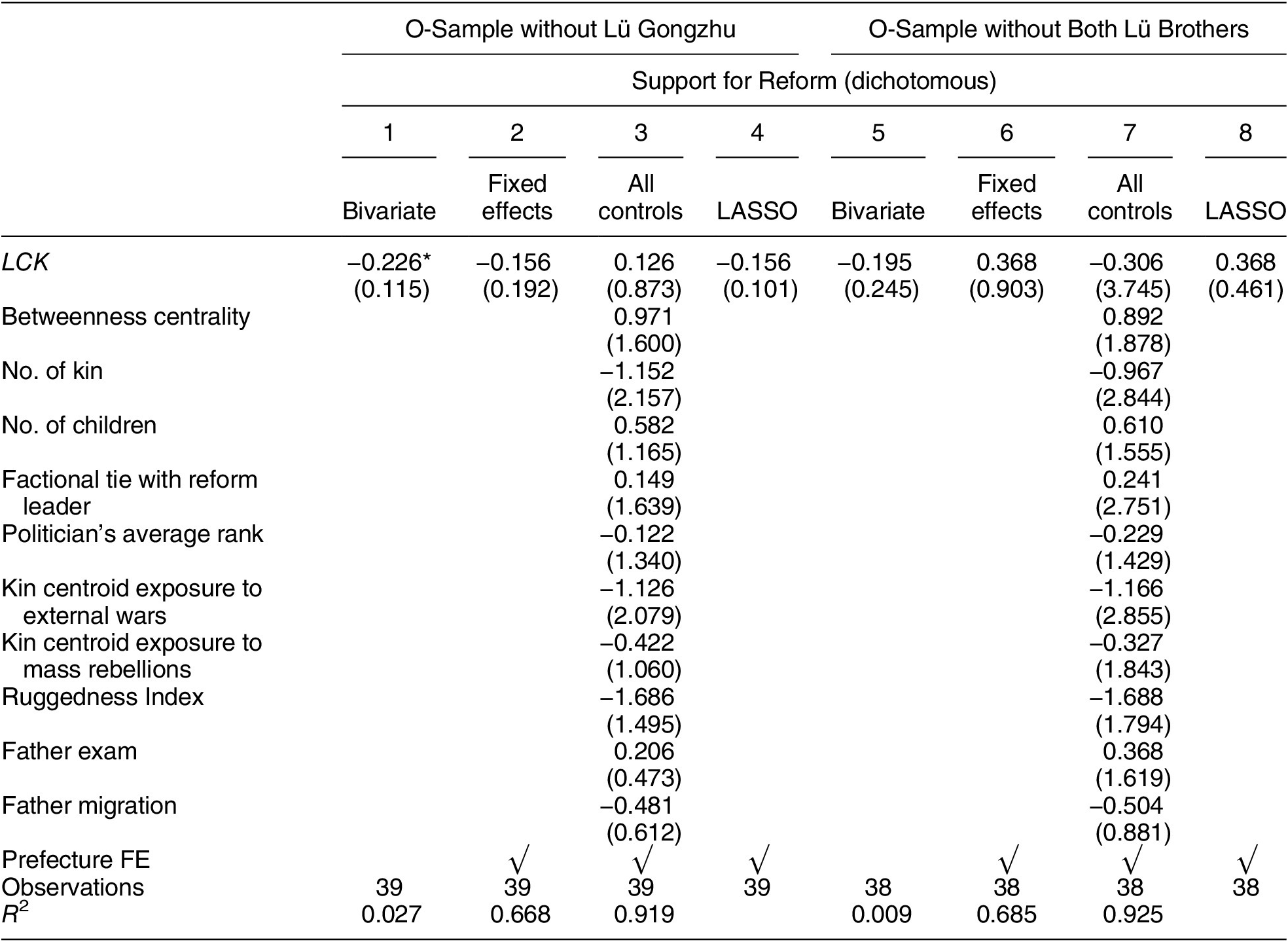
Table 5. Long description
The table is divided into two main sections: O-Sample without Lü Gongzhu (Models 1 to 4) and O-Sample without Both Lü Brothers (Models 5 to 8). Each section includes Bivariate, Fixed effects, All controls, and L A S S O specifications.
Key variables and coefficients:
* L C K: Values range from -0.226 (Model 1, p < 0.10) to 0.368 (Models 6 and 8). Standard errors are provided in parentheses below each coefficient.
* Betweenness centrality: 0.971 in Model 3 and 0.892 in Model 7.
* Number of kin: -1.152 in Model 3 and -0.967 in Model 7.
* Number of children: 0.582 in Model 3 and 0.610 in Model 7.
* Factional tie with reform leader: 0.149 in Model 3 and 0.241 in Model 7.
* Politician’s average rank: -0.122 in Model 3 and -0.229 in Model 7.
* Kin centroid exposure to external wars: -1.126 in Model 3 and -1.166 in Model 7.
* Kin centroid exposure to mass rebellions: -0.422 in Model 3 and -0.327 in Model 7.
* Ruggedness Index: -1.686 in Model 3 and -1.688 in Model 7.
* Father exam: 0.206 in Model 3 and 0.368 in Model 7.
* Father migration: -0.481 in Model 3 and -0.504 in Model 7.
Model Statistics:
* Prefecture F E: Included in Models 2, 3, 4, 6, 7, and 8.
* Observations: 39 for Models 1 to 4; 38 for Models 5 to 8.
* R-squared: Ranges from 0.027 to 0.919 in the first sample and 0.009 to 0.925 in the second sample.
Note: This table replicates BITTW’s estimates (Wang Reference Wang2022, Table 2) with the O-Sample, excluding either Lü Gongzhu alone or both Lü Gongzhu and Lü Gongbi. The unit of analysis is an individual politician. The dependent variable is the politician’s Support for Reform, coded dichotomously. The variable of interest is an index of the local concentration of kin. All variables are standardized. Robust standard errors clustered at the prefectural level are in parentheses. ***p < 0.01, **p < 0.05, *p < 0.10.
OLS Estimates of the Correlation between Geography of Kinship Network and Support for Reform (E-Sample Excluding either Lü Gongzhu or Both Lü Brothers)
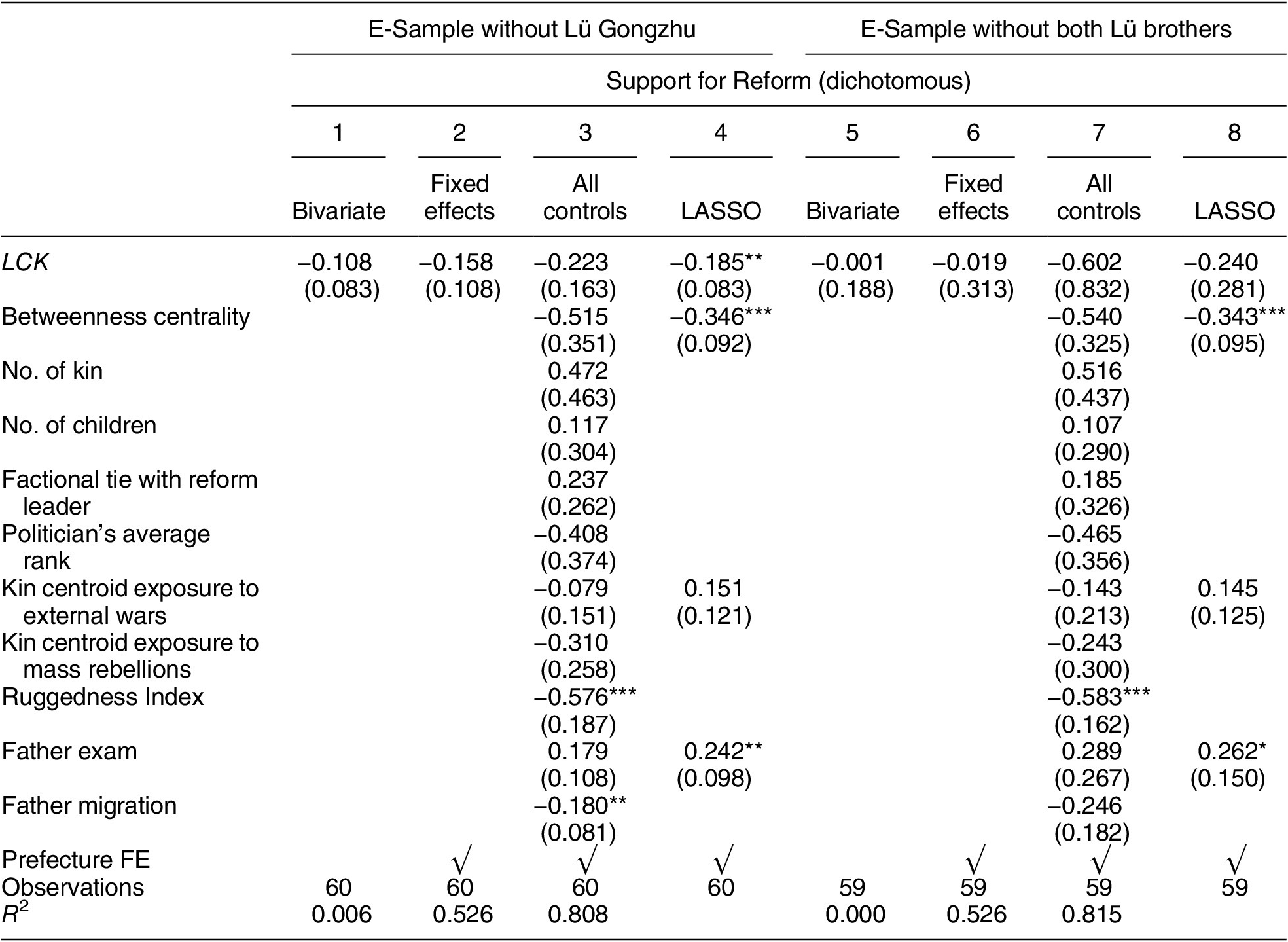
Table 6. Long description
The table presents regression results for Support for Reform across eight models. The columns are divided into two main groups: E-Sample without Lü Gongzhu (Models 1 to 4) and E-Sample without both Lü brothers (Models 5 to 8). Each group includes Bivariate, Fixed effects, All controls, and L A S S O specifications.
Key variables and selected data points:
* L C K: Estimates range from -0.001 to -0.223. The L A S S O model in column 4 shows a significant negative correlation of -0.185 (p < 0.05).
* Betweenness centrality: Shows significant negative correlations in L A S S O models: -0.346 in column 4 and -0.343 in column 8 (both p < 0.01).
* Ruggedness Index: Shows significant negative correlations in the ‘All controls’ models: -0.576 in column 3 and -0.583 in column 7 (both p < 0.01).
* Father exam: Shows positive correlations, significant in L A S S O models: 0.242 in column 4 (p < 0.05) and 0.262 in column 8 (p < 0.10).
* Father migration: Significant negative correlation of -0.180 in column 3 (p < 0.05).
Other variables listed include No. of kin, No. of children, Factional tie with reform leader, Politician’s average rank, Kin centroid exposure to external wars, and Kin centroid exposure to mass rebellions.
The bottom rows indicate:
* Prefecture F E: Included in models 2, 3, 4, 6, 7, and 8.
* Observations: 60 for models 1-4; 59 for models 5-8.
* R-squared: Ranges from 0.000 to 0.815.
Standard errors are provided in parentheses below each estimate. Significance levels are denoted by asterisks: *** p < 0.01, ** p < 0.05, * p < 0.10.
Note: This table replicates BITTW’s estimates (Wang Reference Wang2022, Table 2) with the E-Sample, excluding either Lü Gongzhu alone or both Lü Gongzhu and Lü Gongbi. The unit of analysis is an individual politician. The dependent variable is the politician’s Support for Reform, coded dichotomously. The variable of interest is an index of the local concentration of kin. All variables are standardized. Robust standard errors clustered at the prefectural level are in parentheses. ***p < 0.01, **p < 0.05, *p < 0.10.
RIVAL HYPOTHESES OF PARTISANSHIP GEOGRAPHY
To wit, after improving the sample for the main analysis, the correlation BITTW reported between the geographical dispersal of a politician’s kinship networks and his SFR fails to replicate either when we control for a politician’s hometown region instead of hometown prefecture, or when we exclude an outlier from the relevant sample (in particular, an outlier family from the smaller O-Sample, or an outlier individual from the larger E-Sample). That being said, the E-Sample remains relatively small for statistical purposes, and many important politicians supporting or opposing Reform remain missing from it, spoiling its claim to representativeness. What if, one might wonder, the LCK-SFR correlation reappears when we manage to further expand the sample—say, by unearthing previously unknown tomb epitaphs of Shenzong-era politicians and scraping additional kinship information from them? Would it then rehabilitate BITTW’s theory that geographically dispersed kinship networks incentivize political elites to support the building of a strong state?
Not necessarily. For there are a variety of other issues with BITTW’s analysis, stemming from a combination of the missing-data problem and BITTW’s inadequate engagement with Chinese historical scholarship on Reform’s partisanship geography, that make it ill-prepared to test and defeat rival hypotheses on the role of kinship network dispersal in Reform.
To begin with, the prevailing view among Chinese historians holds that SFR was strongly correlated with a politician’s experience of living (or working) in South China, delimited on the north by “the Huai River, the Tongbai Mountain, the midstream Han River and the Daba Mountains” (Yang Reference Yang1982, 165). That is, politicians who came from South China (or had long stints as magistrates in South China) were likelier to support Reform than their Northern counterparts. Parenthetically, the Southwest (roughly present-day Sichuan and Chongqing) is often carved out for its cultural and economic distinctness at the time, which supposedly turned the few Southwestern Shenzong-era politicians into “moderates” who, while opposing some Reform policies, objected to Northern conservatives’ wholesale opposition to Reform (Liu Reference Liu1959, 28–9).Footnote 31
For understandable reasons (to which I will return later), BITTW’s raw data only contain information on politicians’ hometown prefectures but not on the times and locations of their magistracy experiences. As Table 1 summarizes, among the 61 politicians in the E-Sample, 25 politicians came from the North (“N”), 32 politicians the South (“S”) and four politicians the Southwest (“W”). Table 7 reports, among other things, the OLS estimates of the correlation between a politician’s hometown region and his attitude toward Reform in the E-Sample, controlled for LCK as well as all other variables BITTW used, except prefecture fixed effects. Consistent with the prevailing view, there is a significant correlation between being Southerner/Northerner and being pro-Reform/anti-Reform (while the number of Southwestern politicians in the E-Sample is too low for meaningful results).
OLS Estimates of the Correlation between either Hometown Region or Geography of Kinship Network and Support for Reform (E-Sample)
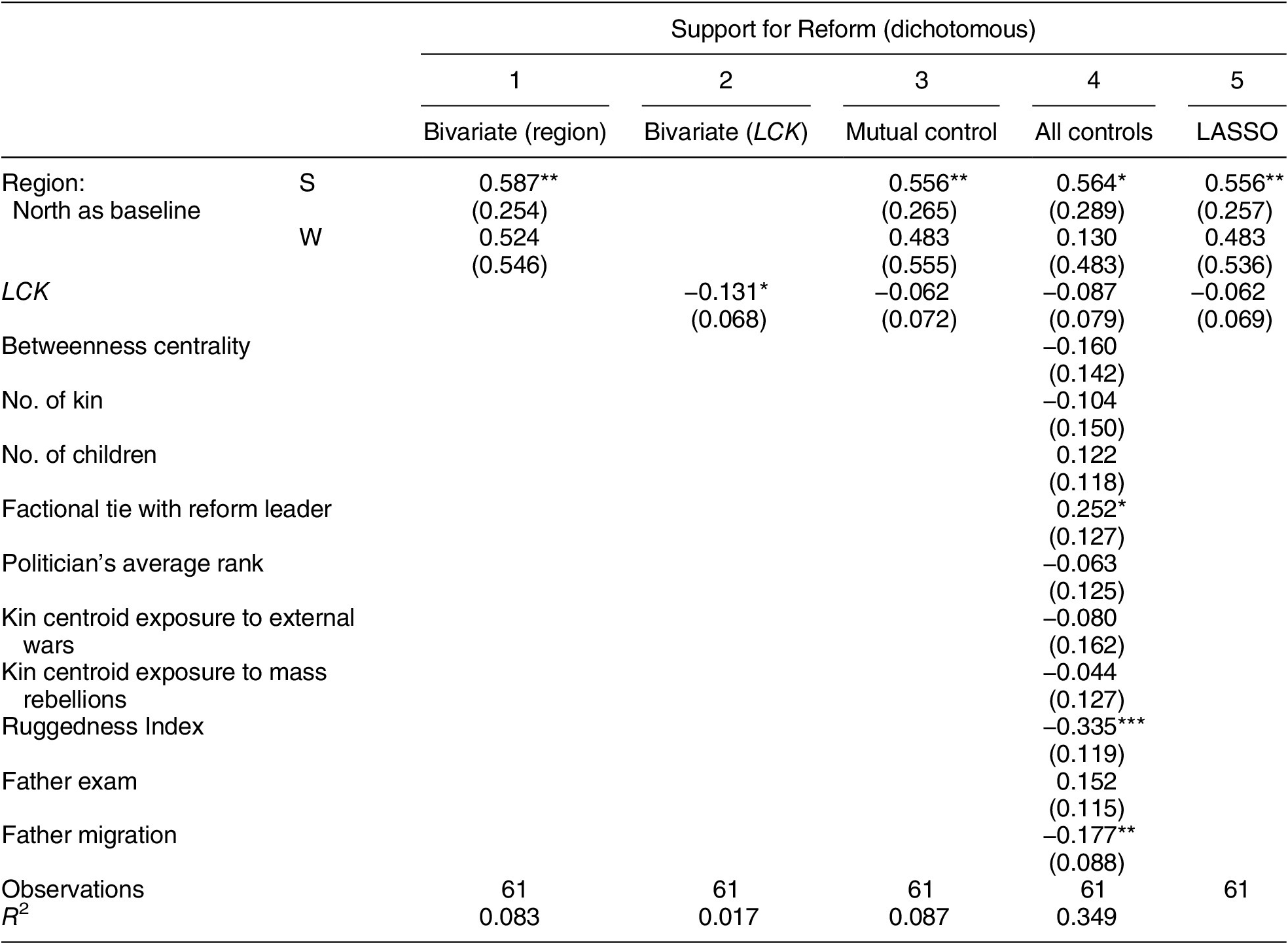
Table 7. Long description
The table presents results for Support for Reform (dichotomous) across five columns: 1 Bivariate (region), 2 Bivariate (L C K), 3 Mutual control, 4 All controls, and 5 L A S S O.
Key variables and coefficients (standard errors in parentheses):
* Region (North as baseline):
- S: 0.587 double asterisk (0.254) in model 1; 0.556 double asterisk (0.265) in model 3; 0.564 asterisk (0.289) in model 4; 0.556 double asterisk (0.257) in model 5.
- W: 0.524 (0.546) in model 1; 0.483 (0.555) in model 3; 0.130 (0.483) in model 4; 0.483 (0.536) in model 5.
* L C K: -0.131 asterisk (0.068) in model 2; -0.062 (0.072) in model 3; -0.087 (0.079) in model 4; -0.062 (0.069) in model 5.
* Significant Controls in Model 4:
- Factional tie with reform leader: 0.252 asterisk (0.127).
- Ruggedness Index: -0.335 triple asterisk (0.119).
- Father migration: -0.177 double asterisk (0.088).
* Other controls in Model 4 (non-significant): Betweenness centrality (-0.160), No. of kin (-0.104), No. of children (0.122), Politician's average rank (-0.063), Kin centroid exposure to external wars (-0.080), Kin centroid exposure to mass rebellions (-0.044), and Father exam (0.152).
* Summary Statistics:
- Observations: 61 for all models.
- R-squared: 0.083 (Model 1), 0.017 (Model 2), 0.087 (Model 3), 0.349 (Model 4).
Note: Asterisks denote p-values: triple asterisk p < 0.01, double asterisk p < 0.05, asterisk p < 0.10.
Note: The unit of analysis is an individual politician. The dependent variable is the politician’s Support for Reform, coded dichotomously. The first variable of interest is the politician’s hometown region—North (N), South (S), or Southwest (W)—with North (N) being the baseline. The second variable of interest is an index of the local concentration of kin. Column 3 uses the two variables of interest as each other’s control. All variables are standardized. Robust standard errors are in parentheses. ***p < 0.01, **p < 0.05, *p < 0.10.
How might this prevailing view bear on BITTW’s subject matter, that is, the relationship between kinship network dispersal and support for state-building? Consider two common explanations of why the South/North divide correlated with the pro-Reform/anti-Reform divide: status competition and policy adaptiveness.
Status Competition
According to the status-competition explanation, whereas the North had been China’s economic, cultural, and political center for much of Chinese history, by the mid-11th century, it was on the brink of being surpassed, for good, by the burgeoning South. Illustratively, the proportion of chancellors who were Southerners rose from 0% in the early years of the Northern Song dynasty (960–997 CE), to 22.2% during Emperor Zhenzong’s reign (997–1022 CE), to 42.1% during Emperor Renzong’s (1022–1063 CE), and then suddenly to 83.3% under the auspices of Emperor Shenzong (1067–1085 CE), reaching the zenith of Southern political power (followed by a purge of Southern chancellors—and Reform’s repeal—soon after Emperor Shenzong’s death) (Yang Reference Yang1982, 166). The rapidly shifting balance in the North/South status competition created an intense animosity between Northern “old guards” and Southern “new arrivals,” fueling—and being fueled by—the latter’s eagerness to exercise their freshly acquired power and the former’s perception of it as usurpation (Liu Reference Liu1959, 37–8). Now, suppose the nouveau riche are more interested in “marrying up” and building social capital than are the old guard in making peace with its challengers, for whom it cannot help feeling contempt. If so, the status-competition explanation implies the following rival hypothesis to BITTW’s on kinship network dispersal:
Rival Hypothesis 1: Southern politicians in the era of Reform tended to have geographically more dispersed kinship networks than Northern politicians.Footnote 32
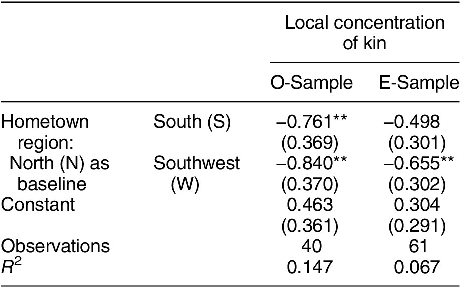
Accordingly, insofar as there is an LCK-SFR correlation, it is not because geographically dispersed kinship networks incentivized politicians to support state-building, but because the South/North divide caused the differences in both the geography of kinship networks and attitudes toward Reform. Interestingly, as Table 8 shows, the correlation between the South/North divide and kinship network dispersal is significant in the O-Sample but insignificant in the E-Sample. Suppose, as speculated above, that the LCK-SFR correlation reemerges in a further expanded sample in the future, the same tests on the effects of the South/North divide both on LCK itself (Table 8) and on the LCK-SFR correlation (Table 7) need to be done too, to determine if BITTW’s theory survives the challenge of this rival hypothesis at all.
OLS Estimates of the Correlation between Hometown Region and Geography of Kinship Network (O-Sample vs. E-Sample)
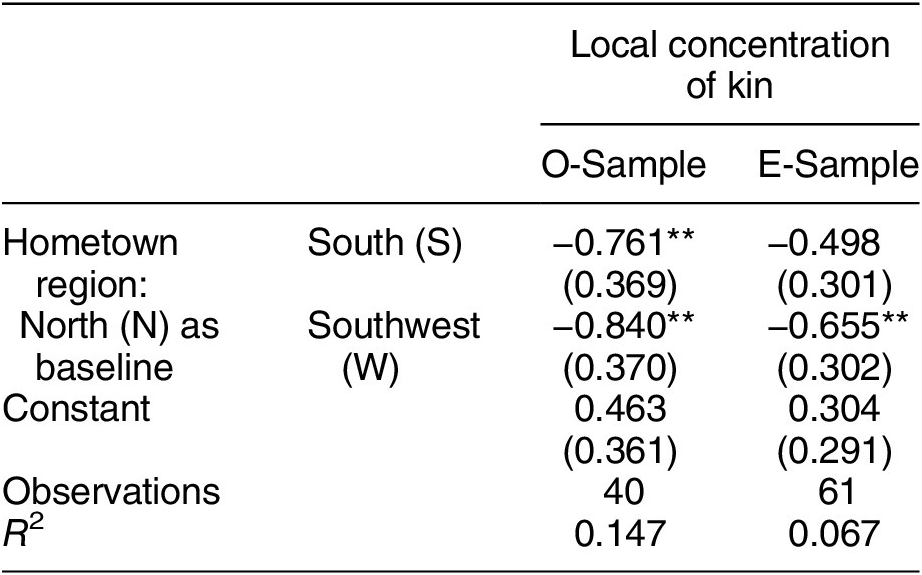
Table 8. Long description
The table compares two groups, O-Sample and E-Sample, regarding the local concentration of kin. The independent variable is Hometown region with North N as the baseline.
* South S: O-Sample shows a coefficient of minus 0.761 with a standard error of 0.369, significant at the p < 0.05 level. E-Sample shows a coefficient of minus 0.498 with a standard error of 0.301.
* Southwest W: O-Sample shows a coefficient of minus 0.840 with a standard error of 0.370, significant at the p < 0.05 level. E-Sample shows a coefficient of minus 0.655 with a standard error of 0.302, significant at the p < 0.05 level.
* Constant: O-Sample is 0.463 with a standard error of 0.361. E-Sample is 0.304 with a standard error of 0.291.
* Observations: O-Sample has 40; E-Sample has 61.
* R-squared: O-Sample is 0.147; E-Sample is 0.067.
All variables are standardized and robust standard errors are provided in parentheses.
Note: The dependent variable is an index of the local concentration of kin. The variable of interest is the politician’s hometown region—North (N), South (S), or Southwest (W)—with North (N) being the baseline. All variables are standardized. Robust standard errors are in parentheses. ***p < 0.01, **p < 0.05, *p < 0.10.
Policy Adaptiveness
According to the policy-adaptiveness explanation, the North and the South were so different in their natural and socioeconomic conditions that no one-size-fits-all Reform package could possibly work in both regions. Meanwhile, the chief architect of Reform, Wang Anshi, who not only grew up in the South but whose magistracy experiences were also confined to South China, was much more versed in Southern conditions than in Northern ones. What’s more, he was by all accounts an adamant and overconfident person unable to take criticism. Consequently, many of his policies were particularly maladapted to the North, provoking vehement Northern opposition. For example, the “hired” labor service reform, with “commutation to cash tax payment” at its core, “worked better in the southern areas where money economy was better developed” but “caused considerable hardship in the northern areas” (Liu Reference Liu1959, 109). As the Chinese proverb goes: tangerines grown south of the Huai River are sweet tangerines, while those grown in the north, due to their different shuitu (“water-and-earth”), become bitter trifoliate oranges.
Compared with other explanations, the policy-adaptiveness explanation is particularly attuned to the nuanced attitudes many politicians held toward Reform: a politician would support one Reform policy and oppose another if the former was adaptive, and the latter was maladaptive, to the local conditions with which he was versed in; and he might change his view on a particular Reform policy, or on Reform as a whole, when he acquired knowledge on the local conditions with which he had not been versed. Meanwhile, it also makes better sense of a fact BITTW did not mention (and could not account for), that many leading opponents of Reform (such as Fu Bi, Han Qi, and Ouyang Xiu) had been whole-hearted supporters of the thwarted Qingli New Deal (1043–1045 CE) two decades before, seeking also to strengthen state capacity. BITTW’s theory implies—quite implausibly—that the “Qingli generation” politicians turned against state-building two decades later because, as time went by, their kinship networks became more concentrated geographically. By contrast, according to the policy-adaptiveness explanation, they opposed Reform not because they opposed state-building per se, but because they deemed it a misinformed package of state-building policies, which its bullheaded architect pushed hastily through. In a nutshell, “anti-Reform” should not be equated with “anti-reform” (i.e., opposing reforms that strengthen state capacity).
Like the status-competition explanation, the policy-adaptiveness explanation begets a rival hypothesis to BITTW’s on kinship network dispersal:
Rival Hypothesis 2: Geographically dispersed kinship networks tended to increase Northern politicians’ Support for Reform, but reduce Southern politicians’ Support for Reform.
A geographically dispersed kinship network could increase a Northern politician’s exposure to Southern local knowledge, as well as a Southern politician’s exposure to Northern local knowledge. Given that Reform was more adaptive to Southern conditions than to Northern conditions, a Northerner with a dispersed kinship network was likelier than a Northerner with a concentrated kinship network to acknowledge that at least some Reform policies worked in certain parts of China, and a Southerner with a dispersed kinship network was likelier than a Southerner with a concentrated kinship network to acknowledge that at least some Reform policies did not work in certain parts of China.Footnote 33 Hence the hypothesis.
It would be a daunting task to test this hypothesis quantitatively, however. To begin with, we ideally must know—and control for—when and where a politician served as a local magistrate, which, like having a dispersed kinship network, might expose him to local conditions different from where he grew up and affect his view on Reform. Sans the influence of one’s kinship network, the timing of his magistracy experience affects how well-versed he already was in various local conditions before expressing or changing his view on Reform (or on any specific Reform policy), and the whereabouts of those experiences could be relevant to his policy-specific attitudes.Footnote 34 Relatedly, we also need as detailed information as possible on politicians’ policy-specific attitudes, as well as on their attitude changes over time. Yet, historical records of the Song dynasty often specified only where, but not when, a politician worked as a magistrate; and as mentioned earlier, it is likely that the data gathered on policy-specific attitudes and attitude changes would also be highly incomplete, even if we were to increase exponentially the time and effort spent on scraping additional information from rare historical sources. In other words, the missing-data problem looms even larger for the quantification of Rival Hypothesis 2 than for BITTW.
THE LIMITS OF QUANTITATIVE HISTORY
So far, we have reached the following conclusions. First, taking the control and outlier issues into account, the results BITTW reported fail to replicate when we mitigate its missing-data problem and improve its sample with the help of additional historical records; but as the missing-data problem is not fully eliminated, there is a theoretical possibility of BITTW being rehabilitated by a further expanded sample. Second, BITTW also fails to engage adequately with the prevailing view in Chinese historical scholarship on Reform’s partisanship geography, which yields statistically significant results on the correlation between the South/North divide and the pro-Reform/anti-Reform divide. Third, two common explanations of this partisanship geography, that is, status competition and policy adaptiveness, give rise to two corresponding alternatives to BITTW’s hypothesis on the role of kinship network dispersal in Reform. The status-competition-based hypothesis is easier to quantify, but it yields uncertain results with the sample at hand. By contrast, due to missing data, the more fine-grained policy-adaptiveness-based hypothesis cannot be properly quantified, despite its greater capacity to explain the various nuances of attitudes toward Reform. All in all, this case perfectly illustrates the inherent limits of quantitative history, which researchers should always keep in mind while wielding this ostensibly powerful tool.
DATA AVAILABILITY STATEMENT
Research documentation and data that support the findings of this study are openly available at the American Political Science Review Dataverse: https://doi.org/10.7910/DVN/IMTK8A.
ACKNOWLEDGEMENTS
I am particularly grateful to Yuhua Wang, whose openness to criticism is exemplary, and to Ye Zhang, who read drafts of this article attentively and spotted several unforced errors in them. In addition, I would also like to thank Yunpeng Bai, Zixi Chen, Siqin Kang, Zhiyu Shang, and Hongbo Wang, as well as the audience of my presentation at the AAS-in-Asia annual conference (Daegu, Korea, June 26, 2023), two anonymous reviewers, and the editors of American Political Science Review, for their comments and suggestions.
CONFLICT OF INTEREST
The author declares no ethical issues or conflicts of interest in this research.
ETHICAL STANDARDS
The author affirms this research did not involve human participants.


 Open access


Comments
No Comments have been published for this article.