





Nomenclature
List of symbols
-
 $A$
-
two-zone temperature parameter
-
$B$
-
two-zone shape function
-
$c$
-
calibration parameter
-
$d$
-
diameter
-
$EGR$
-
exhaust gas recirculation rate
-
$EI$
-
emission index
-
$FAR$
-
fuel-air ratio
-
$h$
-
specific enthalpy
-
$m$
-
mass
-
$M$
-
molar mass
-
$p$
-
pressure
-
$s$
-
unmixedness
-
$SFC$
-
specific fuel consumption
-
$t$
-
time
-
$T$
-
temperature
-
$u$
-
fluid velocity
-
$v$
-
piston velocity
-
$w$
-
mass flow
-
$WAR$
-
water–air ratio
-
$\alpha$
-
combustor air addition profile
-
$\beta$
-
combustor primary zone air split
-
$\lambda$
-
air-excess ratio
-
$\rho$
-
density
-
$\sigma$
-
standard deviation
-
$\tau$
-
timescale
-
$\phi$
-
fuel-air equivalence ratio
$=1/\lambda$
-
$\varphi$
-
crank angle


List of subscripts/superscripts
-
$0$
-
initial / without combustion
-
$1$
-
combusted zone
-
$2$
-
uncombusted zone
-
$3$
-
combustor inlet
-
$a$
-
air
-
$amb$
-
ambient
-
$crit$
-
critical point
-
$dil$
-
dilution
-
$EOC$
-
end-of-combustion
-
$f$
-
fuel
-
$inj$
-
injected
-
$mix$
-
mixing / homogenisation
-
$stoich$
-
stoichiometric
-
$SOC$
-
start-of-combustion
-
$w$
-
water


List of acronyms
- CCE
-
composite cycle engine
- CFD
-
computational fluid dynamics
- EGR
-
exhaust gas recirculation
- EOC
-
end of combustion
- FDP
-
free-double piston
- LTO
-
landing & take-off operations
- LR
-
long-range
- PSR
-
perfectly stirred reactor
-
probability density function
- RQL
-
Rich-burn, quick-mix, lean-burn
- SLS
-
sea-level static
- SAF
-
sustainable aviation fuel
1.0 Introduction
Future propulsion concepts are driven by the need to significantly reduce the climate impact of aviation, while ensuring low fuel consumption for airlines to stay competitive. Among several novel candidates, the composite cycle engine (CCE) concept has been investigated for several years [Reference Kaiser, Seitz, Donnerhack and Lundbladh1, Reference Nickl and Kaiser2]. This concept introduces a piston engine system to the core of a gas turbine engine. While various CCE architectures in both two- and four-stroke configurations, including reciprocating, rotary and free-piston variants, have been investigated, this work is motivated by the so-called free-double piston (FDP) variant. This architecture is of particular interest for its potential lower mass, as it functions strictly as a gas generator without mechanical power provision, utilising an integrated unit of piston compressors and opposite-located engine cylinders that share a single piston element. The FDP solution was first described by Klingels [Reference Klingels3], with a detailed description and its conceptual design implications initially presented by Kaiser et al. [Reference Kaiser, Schmitz and Klingels4].
The closed-volume combustion of the piston engine, as well as the higher cycle peak temperatures and pressures, results in significant improvements in thermal efficiency [Reference Kaiser, Seitz, Donnerhack and Lundbladh1]. When integrated and assessed at the aircraft level, the thermal efficiency benefits translate to healthy double-digit mission fuel burn reductions relative to similarly advanced geared turbofan engines. However, these benefits are accompanied by an increase in system weight and
 $\mathrm{NO}_x$
emissions. As the piston engine is responsible for the bulk of CCE
 $\mathrm{NO}_x$
emissions due to elevated temperatures and pressures, addressing this source is particularly critical for the viability of the concept. As shown by Kaiser et al. [Reference Kaiser, Kellermann, Nickl and Seitz5], CAEP/6-75% targets are projected to be exceeded by the CCE, with cruise-phase emissions being of particular concern due to their disproportionate impact on climate. Effective
 $\mathrm{NO}_x$
mitigation measures are therefore crucial.
Mitigation strategies under consideration include optimisation of valve and injection timings, compression intercooling ahead of the piston system, relocation of fuel injection to the Joule combustor (at the expense of thermal efficiency), application of rich combustion in the piston stage with lean combustion in the Joule combustor (with potential soot formation and high cylinder temperatures) and combustion vitiation (e.g. by gas recirculation or water injection) [Reference Kaiser, Schmitz and Klingels4]. All approaches involve engine- and aircraft-level trade-offs. Exhaust gas recirculation (EGR) and water injection have shown particularly high
 $\mathrm{NO}_x$
reduction potential, as they simultaneously reduce flame temperature and oxygen availability for emission formation. Due to their promising potential in both piston and gas turbine systems [Reference Andreasen and Nyggard6–Reference Muley and Lear8], the impact on
 $\mathrm{NO}_x$
emissions in the CCE is further investigated in this paper.
Nitrogen oxides (
 $\mathrm{NO}_x$
) emitted from internal combustion engines and gas turbines consist primarily of nitric oxide (
 $\mathrm{NO}$
) and nitrogen dioxide (
 $\mathrm{NO}_2$
). While multiple formation pathways exist, including the prompt,
 $\mathrm{N_2O}$
and
 $\mathrm{NNH}$
mechanisms relevant for hydrocarbon-rich, lean-low-temperature or high-pressure, or hydrogen-combustion regimes, respectively [Reference Merker and Teichmann9, Reference Wang and Yang10], the high-temperature environment of the CCE establishes the thermal
 $\mathrm{NO}$
(extended Zeldovich) mechanism as the dominant contributor. Fuel-bound nitrogen and its
 $\mathrm{NO}$
formation path is negligible for standard aviation fuels [Reference Wang and Yang10]. Furthermore, while the high inlet
 $\mathrm{NO}$
concentrations in the CCE Joule combustor suggest potential for
 $\mathrm{NO}$
reburning, a reduction phenomenon observed in vitiated flows that requires more detailed chemistry [Reference Chen, Smoot, Hill and Fletcher11–Reference Glarborg, Kristensen, Dam-Johansen, Alzueta, Millera and Bilbao13], this study adopts a simplified approach by focusing on the gross production via the thermal route. Consequently, the modelling effort is centred on the extended Zeldovich mechanism.
The estimation of
 $\mathrm{NO}_x$
formation requires precise knowledge of local temperatures and species concentrations. The scientific literature categorises the modelling efforts into a hierarchy based on spatial resolution and computational effort. At the highest level of complexity, 3D computational fluid dynamics (CFD) models provide high-fidelity spatial resolution by solving the Navier–Stokes equations, capturing the detailed interaction between turbulent flow, spray evaporation and local chemical kinetics. However, the long computation times required make CFD inadequate for early predesign, which requires estimates over wide parameter sweep studies. Conversely, global correlation-based models, widely used for their simplicity, link global parameters such as inlet conditions and fuel-air ratio (FAR) to experimental datasets. While effective for derivative engines within their calibration range, these models often lack the physical predictive capability required for novel architectures. This is particularly true for piston engines, where the high number of sensitive parameters limits the applicability of simple correlations. To bridge this gap between complexity and utility, quasi-dimensional models have been deployed, segmenting the combustion process into discrete volumes or zones while retaining a physically based representation of the dominant processes. By simulating the thermodynamic history of individual zones, these models capture the local variations in FAR that drive
 $\mathrm{NO}_x$
formation. While multi-zone approaches offer high fidelity in piston engines, they require detailed input data, such as injection rate profiles and spray geometry [Reference Lamaris, Hountalas, Zannis and Glaros14–Reference Weisser16]. Consequently, there is a need for a balanced modelling approach that captures the essential physics of peak temperatures. This is crucial for both piston and Joule combustors, while maintaining the computational efficiency required for system-level studies for the CCE.
This work presents a quasi-dimensional modelling framework for both the piston engine and the Joule combustor, designed to bridge the gap between empirical correlations and high-fidelity simulations. The methodology is demonstrated through studies of
 $\mathrm{NO}_x$
emission in an FDP-CCE, with a particular focus on water injection and EGR. Although the proposed methodology is inherently fuel-agnostic, this work focuses primarily on kerosene-based applications. Additionally, its versatility is demonstrated through a piston engine validation case involving hydrogen (
 $\mathrm{H2}$
).
2.0 Methodology
2.1.
$\mathrm{NO}_x$
kinetics

This study only considers thermal
 $\mathrm{NO}$
formation described by the extended Zeldovich mechanism [Reference Merker and Teichmann9]:
 \begin{align} \mathrm{N}_{2} + \mathrm{O} \stackrel{k_1}{\longleftrightarrow} \mathrm{NO} + \mathrm{N} \end{align}
 \begin{align} \mathrm{N} + \mathrm{O}_{2} \stackrel{k_2}{\longleftrightarrow} \mathrm{NO} + \mathrm{O} \end{align}
 \begin{align} \mathrm{N} + \mathrm{OH} \stackrel{k_3}{\longleftrightarrow} \mathrm{NO} + \mathrm{H} \end{align}
The available concentrations of species
 $\mathrm{N}$
,
 $\mathrm{O}$
and
 $\mathrm{OH}$
at the respective fluid composition and temperature are determined with the
 $\mathrm{OHC}$
-system. The implementation of the extended Zeldovich and the
 $\mathrm{OHC}$
-system, including the determination of the forward and backward reaction rates
 $k_{1-3}$
and validation, is described by Kaiser [Reference Kaiser17].
While
 $\mathrm{NO}$
is the primary species formed and emitted at the engine exhaust, it is unstable in the atmosphere. Over time, practically all exhaust NO oxidises to form nitrogen dioxide (
 $\mathrm{NO}_2$
). Because of this inevitable conversion, environmental regulations standardise the reporting of
 $\mathrm{NO}_x$
emissions. Regardless of the actual ratio of
 $\mathrm{NO}$
to
 $\mathrm{NO}_2$
at the tailpipe, the total mass of
 $\mathrm{NO}_x$
is calculated using the molar mass of
 $\mathrm{NO}_2$
[18]:
 \begin{align} m_{NO_x} = n_{NO} \cdot M_{NO_2} \end{align}
The
 $\mathrm{NO}_x$
mass results from the number of
 $\mathrm{NO}$
moles
 $n_{NO}$
and the molar mass
 $M_{NO_2} = 46.0055\,g/mol$
. The
 $\mathrm{NO}_x$
results in this work are given with the emission index, which relates
 $\mathrm{NO}_x$
mass to fuel burn mass as
 $EI\,NO_x = m_{NO_x}/m_f$
.
2.2. Piston
$\mathrm{NO}_x$
model

The piston system is modelled in an in-house tool, capable of calculating different types of piston compressors and engines. This includes the performance calculation and the
 $\mathrm{NO}_x$
emissions calculations, whereas the latter is estimated as a post-processing step.
For the performance calculation, the piston engine is described by a zero-dimensional, single-zone model, resolving the thermodynamic performance in timesteps, commonly defined by crank angle for one full revolution of the cycle. The combustion process is described with the empirical Wiebe function, where two Wiebe parameters (
 $w_a$
and
 $w_m$
) are applied to describe the heat release rate [Reference Wiebe19]. The
 $w_a$
parameter defines the fuel burn utilisation. In the default setup,
 $w_a$
is set to 6.908 for lean combustion, representing 99.9% of combustion efficiency. In the present predesign study,
 $w_a$
is kept constant for lean operating points, which assumes stable and nearly complete combustion. This is considered appropriate for the investigated operating range, but may become optimistic for very lean mixtures, where incomplete combustion or combustion instability effects could reduce the actual fuel-burn utilisation. For a rich, oxygen-limited operation,
 $w_a$
is reduced according to the availability of oxygen. For the heat transfer from the hot gas to the cylinder wall, several semi-empirical models were tested and calibrated with the crankshaft-based engine described by Van Gerpen [Reference Van Gerpen20]. After comparison of the overall performance and main cycle parameter evolutions, the correlation given by Hohenberg [Reference Hohenberg21] is selected, as it best matches the overall piston engine performance. A calibration factor of
 $0.64$
is applied to the Hohenberg heat-transfer model to best reproduce the reference engine performance. Since the correlation does not explicitly account for high-wall-temperature heat transfer effects, their influence on the predicted cylinder-temperature history remains a modelling uncertainty. Neglecting such effects is expected to be conservative with respect to thermal
 $\mathrm{NO}$
formation, as enhanced wall heat transfer would tend to lower peak gas temperatures. For more details on the piston system modelling, the reader is referred to Kaiser [Reference Kaiser17] and Lin et al. [Reference Lin, Uhl, Winter, Lessis, Witzgall and Seitz22]. Analogous modelling for hydrogen fuel has been described by Nickl et al. [Reference Nickl, Winter and Gümmer23] and Winter et al. [Reference Winter, Lin, Nickl and Seitz24]. Due to the absence of soot in hydrogen combustion, which acts as an insulator in internal combustion engines, a modified Woschni correlation [Reference Gerstle25] is used with a calibration factor of 3.3 to reflect this phenomenon. In addition, the combustion duration is shortened compared with the kerosene variant to represent the shorter combustion times associated with hydrogen operation.
2.2.1. Model description
Single-zone models capture only the mean cylinder temperature and composition and are thereby insufficient to describe hot cylinder regions that are crucial for
 $\mathrm{NO}_x$
formation. In contrast to multi-zone models, the two-zone approach simplifies the combustion chamber into two distinct thermodynamic domains: the unburned and the burned (combusted) zones. These regions are separated by an infinitely thin flame front, which is typically not explicitly modelled due to its negligible volume and limited direct impact on the global kinetics of
 $\mathrm{NO}$
formation.
The primary differentiation among two-zone methodologies lies in their initialisation of these domains and the mechanisms used to describe their interaction. Li et al. [Reference Li, Zhu and Men26] present a two-zone reaction-based combustion model that accounts for both heat and mass exchange between the zones. The model described by Kozuch [Reference Kozuch27] includes a detailed mixing model, solving a global homogeneous isotropic
 $k-\epsilon$
model to resolve cylinder turbulence. Similar approaches to calculate in-cylinder turbulence to determine mixing are given by Andersson et al. [Reference Andersson, Johansson, Hultqvist and Noehre28] and Brückner et al. [Reference Brückner, Pandurangi, Kyrtatos, Bolla, Wright and Boulouchos29]. Heider et al. [Reference Heider, Woschni and Zeilinger30] instead describe a more empirical two-zone model that only requires few engine-specific input parameters. Oppenauer and Del Re [Reference Oppenauer and Del Re31] combine the Heider approach with the parallel mixing model of Kozuch [Reference Kozuch27]. The authors also highlight that pure physical models are difficult to adapt, especially to modern diesel engines, as the required calibration parameters vary during operation.
In the following, the two-zone model implementation is described, as it proved sufficiently accurate while requiring a minimum amount of unknown setup parameters. The fundamental logic originates from Heider et al. [Reference Heider, Woschni and Zeilinger30], with the implementation most closely resembling Kaiser [Reference Kaiser17].
Schematic of the two-zone mass balance.

Figure 1 visualises the two-zone mass balance, which is described in mathematical terms through Equations (5–9). The cylinder mass is partitioned into a burned (
 $1$
) and unburned zone (
 $2$
),
 \begin{align} m_{total} = m_1 + m_2, \end{align}
where
 $m_1$
and
 $m_2$
are the two zone masses. The fuel-air ratio of the burned zone
 $FAR_1$
is defined by the air-excess ratio
 $\lambda _0$
and the stoichiometric
 $FAR_{stoich}$
:
 \begin{align} FAR_1 = \dfrac {FAR_{stoich}}{\lambda _0} \end{align}
The effect of vitiated inlet air and incomplete scavenging is represented through background fuel and water contents in the incoming charge. These background quantities define the initial
 $FAR_0$
and
 $WAR_0$
, which are constant across both zones. Directly injected fuel
 $m_{f,inj}= m_f - m_{f,0}$
and water
 $m_{w,inj} = m_w - m_{w,0}$
are added only to the combusted zone, resulting in the burned zone composition
 $FAR_1$
and
 $WAR_1$
. Consequently, a change in
 $FAR_0$
alone does not alter
 $FAR_1$
; instead, the amount of freshly burned fuel and the corresponding heat release are determined by the difference
 $FAR_1-FAR_0$
. This difference defines the air mass
 $m_{a,1}$
participating in combustion.
 \begin{align} m_{a,1} = \dfrac { m_{f,inj} }{ FAR_1 - FAR_0 } \end{align}
 \begin{align} WAR_1 = \dfrac {m_{w,inj}}{m_{a,1}} + WAR_0 \end{align}
 \begin{align} m_1 = m_{a,1} \cdot (1 + FAR_1 + WAR_1) \end{align}
Heider et al. [Reference Heider, Woschni and Zeilinger30] give a simple model for the temperature difference between the burned and unburned zones.
 \begin{align} T_1 - T_{2} = B(\varphi ) \cdot A \end{align}
The shape function
 $B(\varphi )$
describes the evolution of the temperature difference along the crank angle
 $\varphi$
and gives an estimate for the energy interaction between the two zones based on pressure evolution,
 \begin{align} B(\varphi ) = 1 - \dfrac { \int _{\varphi _{SOC}}^{\varphi } ( p(\varphi )-p_0(\varphi ) ) \, m_1(\varphi ) \, d\varphi }{ \int _{\varphi _{SOC}}^{\varphi _{EOC}} ( p(\varphi )-p_0(\varphi ) ) \, m_1(\varphi ) \, d\varphi }, \end{align}
with
 $p(\varphi )$
being the cylinder pressure and
 $p_0(\varphi )$
the pressure without combustion. SOC and EOC refer to start and end of combustion.
The factor
 $A$
is described by Heider et al. [Reference Heider, Woschni and Zeilinger30] as an engine-specific calibration temperature difference. Oppenauer and Del Re [Reference Oppenauer and Del Re31] extend
 $A$
to be variable with swirl and EGR. Kaiser [Reference Kaiser17] describes the same approach as chosen here, where
 $A$
is defined as a temperature difference based on the adiabatic flame temperature.
 \begin{align} A = c_A \, (T_{flame} - T_{SOC}) \end{align}
The adiabatic flame temperature
 $T_{flame}$
is established via an enthalpy balance between
 $SOC$
conditions and the flame conditions given by
 $FAR_1$
,
 $WAR_1$
and the water injection temperature
 $T_{w,inj}$
. Compared with the original Heider formulation, this definition reduces the calibration burden on
 $c_A$
, since the temperature difference
 $T_{flame}-T_{SOC}$
already accounts for changes in mixture composition, vitiation, water addition and SOC thermodynamic conditions.
To calculate the zone temperatures, an enthalpy balance ensures energy conservation,
 \begin{align} m_{total} \, h_{total} = m_{1} \, h_{1} + m_2 \, h_2, \end{align}
with the specific enthalpies
 $h$
resulting from the temperature, pressure and composition in the zones.
2.2.2. Calibration and validation
The described methodology results in two calibration parameters. The air-excess ratio
 $\lambda _0$
captures the amount of air added to the burned zone, with
 $\lambda _0=1$
describing stoichiometric combustion. An increase of
 $\lambda _0$
will initially result in an increase in
 $\mathrm{NO}$
as the increased availability of oxygen outweighs the decrease in flame temperature. As
 $\lambda _0$
moves further away from stoichiometric conditions, the predictive capability of a single representative value decreases since in a real engine,
 $\mathrm{NO}$
formation is governed by a distribution of local equivalence ratios, temperatures and radical concentrations rather than by a spatially uniform-burned zone composition. Rich and lean regions will differently impact
 $\mathrm{NO}$
formation due to the availability of radicals. For direct injection, a single
 $\lambda _0$
near stoichiometry has been shown to be capable of providing a good
 $\mathrm{NO}$
estimate. For premixed conditions, the predictions will be less accurate.
The parameter
 $c_A$
scales the initial zone temperature difference, with
 $c_A=1$
resulting in
 $T_1(\varphi _{SOC})=T_{flame}$
. Brückner et al. [Reference Brückner, Pandurangi, Kyrtatos, Bolla, Wright and Boulouchos29] found that actual peak temperatures in conventional diesel combustion typically remain approximately
 $150 \, K$
below the adiabatic flame temperature. However, the authors also find that peak temperatures approach or even surpass this limit in premixed-dominated regimes. This convergence is primarily driven by reduced mixing rates and the compression heating of post-flame gases, which counteracts the thermal dissipation typically seen in diffusion flames. Andreasen and Mayer [Reference Andreasen and Mayer32] reduce the calculated flame temperature by approx
 $100\,K$
via heat radiation. During validation
 $c_A=0.9$
was found to result in decent
 $\mathrm{NO}_x$
trends while the resulting reduction in
 $A$
matched the above-cited temperature ranges.
While in this study
 $c_A$
was kept constant, one could make a case to modify it for a reason other than simply the difference between adiabatic flame temperature and actual hot gas temperature. Although the Heider two-zone model accounts for inter-zone energy transfer via the shape function
 $B$
(Equation 11), it does not explicitly resolve the finite-rate turbulent mixing or local mixture stratification. Under high-pressure, high-temperature conditions close to stoichiometry,
 $\mathrm{NO}$
formation may therefore approach equilibrium rapidly. In such cases, the simplified treatment of mixing and stratification may cause the calculated
 $\mathrm{NO}$
concentration to become limited by equilibrium during the peak-temperature period. Consequently,
 $\lambda _0$
is typically adjusted empirically to match experimental
 $\mathrm{NO}$
results. While this may suffice for part-load studies, it can result in an underestimation of
 $\mathrm{NO}_x$
reduction when evaluating advanced mitigation strategies, such as water injection. In such cases, the model may fail to show the expected
 $\mathrm{NO}$
reduction from flame temperature cooling because the predicted concentrations initially remain equilibrium-limited. As
 $c_A$
directly affects peak temperature, it could be used as a proxy in calibration to limit the extent to which
 $\mathrm{NO}$
formation becomes equilibrium-controlled. In the present study, however, it is kept constant, as satisfactory agreement with literature data was obtained and, given the uncertainty inherent to predesign studies, a physically well-founded justification for its adjustment would be difficult.
The chosen validation engines and calibration parameters are presented in Table 1. To validate the described piston
 $\mathrm{NO}_x$
model, crankshaft-based engines have been set up due to the lack of sufficiently detailed data on free piston engines. The performance setups were tuned to closely align with available data, such as temperature or pressure evolutions and integral metrics such as power or specific fuel consumption
 $SFC$
. Subsequently,
 $\lambda _0$
was tuned for best alignment with literature data, while
 $c_A$
was kept constant. In addition to the diesel part-load studies, previously shown by Kaiser [Reference Kaiser17], an
 $\mathrm{H2}$
engine and vitiated air studies were added.
Overview of piston engine setups used for validation

Table 1. Long description
A table comparing piston engine setups for validation. The table has four rows and four columns. The columns are labeled Engine, Stroke, Bore, and lambda_0. The row labels are Diesel MAN B&W 4T50ME, Diesel Large Generator, and H2 Lombardini 15LD500. Row 1: Diesel MAN B&W 4T50ME, 2, 0.5, 1.093. Row 2: Diesel Large Generator, 2, 0.58, 1.060. Row 3: H2 Lombardini 15LD500, 4, 0.087, 1.005.
1[Reference Andreasen and Nyggard6, Reference Raptotasios, Sakellaridis, Papagiannakis and Hountalas15, Reference Scappin, Stefansson, Haglind, Andreasen and Larsen33].
2[Reference Lamaris, Hountalas, Zannis and Glaros14].
3[Reference Sfriso, Berni, Fontanesi, d’Adamo, Breda, Teodosio, Frigo and Antonelli34, Reference Simi35].
Figure 2 shows the load and EGR (at
 $75\,\%$
load) study for the MAN B&W 4T50ME-X. The model captures the power-specific
 $\mathrm{NO}_x$
emissions well across various loads. However, an underestimation of specific emissions decrease with increasing load can be observed. This decrease is likely a result of the improved mixing at higher engine speeds, which is not captured by the model. For the EGR study, the inlet
 $FAR$
was calculated for each
 $EGR$
value on a dry volume basis, as described by Andreasen and Nyggard [Reference Andreasen and Nyggard6]. The model captures the trend generally well, with the exception of high
 $EGR$
values. The experimental setup utilised an exhaust gas scrubber that cools the recirculated air and removes significant amounts of water, resulting in dry EGR. Because the
 $FAR$
definition of the model inherently includes combustion-product water, it cannot currently simulate a fully dry recirculation path. This is the likely reason for the higher emission reduction predicted with
 $EGR$
, where the additional increase in specific heat capacity of the recirculated water has a substantial effect on the flame temperature and thereby
 $\mathrm{NO}$
formation. For the aeronautical application only wet EGR will be considered.
 $\mathrm{NO}_x$
predictions for the MAN B&W 4T50ME-X (a) load and (b) EGR study.

Figure 3a shows the
 $\mathrm{NO}_x$
emission predictions for the MAN B&W 4T50ME-X operating with water-in-fuel emulsion at
 $75\,\%$
load. In contrast to the experiment, water is not premixed with the fuel in the model; instead, it is introduced into the cylinder at
 $298.15$
K, with the mass flow determined by the fuel flow and the specified water-fuel ratio (
 $WFR$
). The model predicts a linear increase in specific fuel consumption (
 $SFC$
) due to the thermodynamic penalty of heating the water to cylinder temperatures and the associated latent heat of vaporisation (Figure 3b). The experimental results [Reference Andreasen and Nyggard6] show a less pronounced
 $SFC$
increase at moderate
 $WFR$
and even report
 $SFC$
improvements at lower loads. The authors suggest this effect could result from an effective fuel nozzle optimisation due to the added mass flow. At low
 $WFR$
, the model predicts a gradual
 $\mathrm{NO}_x$
reduction, highlighting the sensitivity of the model to the transition between equilibrium-controlled and kinetically limited
 $\mathrm{NO}$
formation. At higher
 $WFR$
,
 $\mathrm{NO}$
formation becomes clearly kinetically limited, and the model’s predicted reduction slope closely matches the experimental trends.
 $\mathrm{NO}_x$
and
 $SFC$
predictions for the MAN B&W 4T50ME-X water-in-fuel emulsion study.

Figure 4a depicts the load study of the large diesel generator described by Lamaris et al. [Reference Lamaris, Hountalas, Zannis and Glaros14]. The model shows good alignment at high load but underestimates the
 $\mathrm{NO}_x$
emissions at lower load. For the small
 $\mathrm{H_2}$
engine at
 $2500$
rpm shown in Figure 4b, the model captures the trend of increasing
 $\mathrm{NO}_x$
emissions with equivalence ratio but fails to capture the high emissions for
 $\phi =0.6$
. Sfriso et al. [Reference Sfriso, Berni, Fontanesi, d’Adamo, Breda, Teodosio, Frigo and Antonelli34] show that the early injections in this engine result in a wide distribution of local equivalence ratio. The distributions change with global
 $\phi$
and engine speed. For
 $\phi =0.6$
at high engine speed, the local equivalence ratios reach up to stoichiometry. This shows one limitation of the model, where the single equivalence ratio choice for the combusted zone fails to capture the wide distribution of the actual conditions.
 $\mathrm{NO}_x$
prediction for (a) the large generator load study [Reference Lamaris, Hountalas, Zannis and Glaros14] and (b)
 $\mathrm{H_2}$
4-stroke Lombardini 15LD500 [Reference Simi35].

Overall, the piston
 $\mathrm{NO}_x$
model shows to be capable of predicting general
 $\mathrm{NO}_x$
trends in the studied piston engines well, including water injection and EGR. For the large two-stroke diesel engines, good alignment with a higher
 $\lambda _0$
of
 $1.06$
and
 $1.093$
was found. These result in a higher
 $\mathrm{NO}_x$
than at the stoichiometric setting due to air entrainment. However, the small four-stroke
 $\mathrm{H}_{2}$
engine calibration resulted in a near-stoichiometric combusted zone with
 $\lambda _0=1.005$
. The previous application of this two-zone model [Reference Kaiser17] showed two smaller four-stroke engines with
 $\lambda _0$
at
 $1.01$
and
 $1.03$
. While these ranges might imply a dependency on the engine cycle (two-stroke vs. four-stroke), here it is argued that engine scale and speed are the more physically relevant factors. In large-bore engines, larger physical mixing scales and slower speeds favour a broader, leaner bulk
 $\mathrm{NO}_x$
production zone. Conversely, in small-bore engines, regardless of cycle architecture, rapid mixing tends to restrict high-temperature
 $\mathrm{NO}_x$
production to narrow, near-stoichiometric interfaces.
Consequently, for the smaller-bore two-stroke FDP engine evaluated in this study,
 $\lambda _0=1$
is adopted. This choice prioritises the physical similarities in mixing dynamics with small four-stroke engines over the nominal similarity in cycle architecture with large diesel engines. While this hypothesis provides a consistent physical basis for this study, further validation, preferably with a two-stroke, small-bore, free-piston engine, is recommended. Within the defined scope, the model is considered sufficient to capture the general trends in the investigated CCE.
2.3. Joule combustor
$\mathrm{NO}_x$
model

2.3.1. Model description
Similar to the piston engine, the fundamental difficulty of gas turbine
 $\mathrm{NO}_x$
modelling lies in the extreme temperature sensitivity of the thermal NO mechanism. The rate of formation scales exponentially with temperature; consequently, the majority of NO is produced in local regions where the equivalence ratio is near stoichiometric (
 $\phi \approx 1$
), even if the global mixture is lean. Traditional zero-dimensional (0D) models that assume a perfectly stirred reactor (PSR) based on average inlet conditions often fail to capture this reality. They tend to substantially underpredict NO formation at lean operating points.
To resolve the combustor mixture without solving the 3D Navier–Stokes equations, stochastic descriptions of the flow field have been introduced [Reference Fletcher and Heywood36, Reference Heywood and Mikus37]. This methodology assumes that while the spatial location of a fuel pocket is unknown (0D/1D approximation), the probability of finding a fluid element at a specific equivalence ratio can be mathematically defined. The key aspects for these models are the stochastic description of the local equivalence ratio and its time evolution.
The stochastic distribution of the local equivalence ratio (
 $\phi$
) can be described by a probability density function (PDF). Heywood and Mikus [Reference Heywood and Mikus37] assume a Gaussian distribution, while other distributions such as
 $\beta$
-PDFs could offer more flexibility if supporting data is available. Heywood and Mikus also consider the stochastic distribution of the local residence time in the primary zone. The fluid homogenises with time, which is of key interest to
 $\mathrm{NO}_x$
formation. This can be captured by sectioning of the combustion chamber into zones with different roles. Heywood and Mikus [Reference Heywood and Mikus37] consider a primary zone without any mixing and a secondary zone where cooling air dilutes the richer primary zone gases and quickly freezes the NO formation process. Therefore they only consider primary zone formation, while noting that this assumption fails if a substantial part of the primary zone flow is fuel rich. Fletcher and Heywood [Reference Fletcher and Heywood36] consider an intermediate zone after the primary zone where homogenisation of the standard deviation takes place proportional to
 $\sqrt {t}$
. In the following dilution zone no further NO formation is assumed. Dederichs et al. [Reference Dederichs, Zarzalis, Habisreuther, Beck, Prade and Krebs38] assume an exponential decrease of the standard deviation with respect to a characteristic time, which was established by means of a reacting large eddy simulation (LES).
The strength of such a stochastic approach is its ability to decouple the macro-scale fluid dynamics from the micro-scale mixing and describing these with a limited number of physical parameters. The assumed PDF can easily be modified to allow for more control over the flow mixedness. This allows quick calibration to different combustor designs, while keeping computational costs low. However, no description for an appropriate cooling air addition model, which is critical to e.g. rich-burn, quick-mix, lean-burn (RQL) combustors, was found in the literature. In the following an implementation for such a stochastic model is described, including the novel adaption to RQL-type combustors. The foundational model could also be adapted to other advanced combustion concepts, such as lean direct injection or staged combustion, which would be an interesting area for future research.
This model simplifies the spatial considerations by assuming only one zone with both homogenisation of the mixture and mixing with the cooling air. To account for the imperfect mixing of fuel and air, the methodology employs a Gaussian (normal) PDF to describe the distribution of local equivalence ratio
 $\phi$
within the combustor, following the description by Heywood and Mikus [Reference Heywood and Mikus37],
 \begin{align} f(\phi ) = \dfrac {1}{\sigma \sqrt {2 \pi }} \cdot exp \left [ - \dfrac {(\phi -\bar {\phi })^2}{2 \sigma ^2} \right ], \end{align}
where
 $\sigma$
is the standard deviation. The mixing quality is quantified by the unmixedness parameter
 $s$
, defined as the ratio of the standard deviation
 $\sigma$
to the mean equivalence ratio
 $\bar {\phi }$
:
 \begin{align} s = \dfrac {\sigma }{\bar {\phi }} \end{align}
The evolution of mixture inhomogeneity is modelled as an exponential decay, described by a characteristic mixing timescale
 $\tau _{mix}$
and the initial unmixedness
 $s_0$
[Reference Dederichs, Zarzalis, Habisreuther, Beck, Prade and Krebs38]:
 \begin{align} s(t) = s_0 \cdot exp \left ( - \dfrac {t}{\tau _{mix}} \right ) \end{align}
The mean equivalence ratio
 $\bar {\phi }$
is determined by the injected fuel mass and the cumulative air addition profile
 $\alpha (t)$
. Only a part of the inlet air is directly routed into the primary zone. This split is described by the assumed inlet air split
 $\beta$
:
 \begin{align} \beta = \dfrac {w_{t=0}}{w_{inlet}} \end{align}
Here,
 $w_{t=0}$
refers to the mass flow in the combustor at start of simulation and
 $w_{inlet}$
is the inlet mass flow from the upstream component.
To capture the quick quenching required in RQL combustors, the cooling air dilution is modelled with a squared exponential based on a characteristic dilution timescale
 $\tau _{dil}$
. This phenomenological formulation assumes all cooling air to be added within this quick mixing. In real combustors a substantial fraction of the cooling air is added continuously for dilution towards the combustor exit, but the assumption is made that this has little influence on
 $\mathrm{NO}$
formation, as it is frozen by the quenching. The cumulative air addition profile
 $\alpha$
at time
 $t$
is defined as
 \begin{align} \alpha (t) = \left\{\begin{array}{l@{\quad}l} \beta & {} {\rm for\ } 0 \leq t \leq \tau _{primary} \\[5pt] \beta + (1 - \beta ) \cdot \left ( 1 - exp\left [- \left (\dfrac {t-\tau _{primary}}{\tau _{dil}}\right )^2 \right ] \right ) {} & {\rm for\ } t \gt \tau _{primary} \end{array}\right \}, \end{align}
with
 $\tau _{primary}$
describing the length of the rich, primary zone ahead of quenching.
The dilution
 $\tau _{dil}$
, the mixing timescale
 $\tau _{mix}$
and the primary zone time
 $\tau _{primary}$
are dependent on engine operation. As done by Dederichs et al. [Reference Dederichs, Zarzalis, Habisreuther, Beck, Prade and Krebs38], the timescales are estimated with calibration parameters
 $c_{dil}$
,
 $c_{mix}$
or
 $c_{primary}$
, the bulk flow velocity
 $u_{bulk}$
and a characteristic length (here the nozzle diameter is used).
 \begin{align} \tau _i = c_i \, \dfrac {d_{nozzle}}{u_{bulk}} = c_i \, \dfrac {\rho \, A_{combustor} \, d_{nozzle}}{\dot {m}} \end{align}
 $A_{combustor}$
refers to the annular cone flow area after the injector including the cooling ducts. The nozzle diameter
 $d_{nozzle}$
serves as a characteristic diameter for the premixing passage.
2.3.2. Discretisation
The flow field is discretised both temporally and stochastically with respect to the local fuel–air equivalence ratio
 $\phi$
. The stochastic discretisation segments the PDF given by Equation (14) into a set of parcels, with each parcel representing the same fixed fraction of the fuel mass flow (see Figure 5a). The respective air mass then results from the local
 $\phi$
obtained from the inverse cumulative distribution function of
 $f(\phi )$
. Total mass conservation is ensured through appropriately scaled parcels.
Joule combustor
 $\mathrm{NO}_x$
model (a) discretisation visualisation and (b) discretisation sensitivity.

The discretisation sensitivity is displayed in Figure 5b. Noteworthy is the high sensitivity to the timestep highlighting the time-sensitive nature of thermal
 $\mathrm{NO}$
formation. The number of parcels is less impactful on
 $\mathrm{NO}_x$
with little difference between
 $30$
and
 $40$
parcels. Accordingly
 $30$
parcels and timestep intervals of
 $0.1$
ms are selected as they lie within
 $4\%$
of the highest-resolved setting while minimising computational cost. Due to the sensitive calibration, this deviation is secondary. Calculation times are then typically well within a second.
The temperature in each parcel and timestep is calculated from a flame temperature calculation via enthalpy balance to inlet conditions given the local
 $\phi$
. Effects of vitiated air, as in the case of the precombusted air in the CCE, are captured by the inlet conditions, which propagate into the combustor. The thermal
 $\mathrm{NO}$
formation at each timestep and parcel is calculated as previously described in subsection 2.1.
2.3.3. Calibration and validation
The proposed model integrates outputs from a gas turbine performance simulation as primary boundary conditions. Specifically, it requires the inlet mass flow, pressure, temperature, FAR and water–air ratio (WAR), alongside the total fuel mass added. Furthermore, the chemical and mixing evolution within the combustor is defined by a number of parameters: the inlet air split
 $\beta$
, representing the initial equivalence ratio; the initial unmixedness
 $s_0$
; and the characteristic timescales for internal homogenisation
 $\tau _{mix}$
, dilution
 $\tau _{dil}$
and the primary zone
 $\tau _{primary}$
. While these timescales are derived from specific calibration constants, as described by Equation (19), their physical significance and representative values from the literature are discussed in the following section.
The inlet air split
 $\beta$
represents the fraction of total combustor air directed into the primary reaction zone. It establishes the initial stoichiometry, dictating the base level of thermal
 $\mathrm{NO}$
production before any secondary dilution or internal mixing occurs and whether later the stoichiometric region needs to be crossed. The upper bound of
 $\beta$
is typically constrained by the lean flammability limit. In staged combustion systems, a lightly loaded primary zone may operate at an equivalence ratio of approximately
 $0.8$
during low-power conditions to ensure high combustion efficiency and minimise CO and unburned hydrocarbon (UHC) emissions. Conversely, at full-load conditions, the primary zone
 $\phi$
is often lower, at around
 $0.6$
, to mitigate
 $\mathrm{NO}_x$
formation as the secondary zone becomes active ([Reference Lefebvre and Ballal39], pp. 24–25). RQL combustors show an even higher initial equivalence ratio (1.2–1.6 [Reference Lefebvre and Ballal39]) and rely on quick mixing. Smith [Reference Smith40] reports a primary zone equivalence ratio of about
 $2$
for the V2500-A5 combustor at 100% load, with only 19% and 7% of total combustor air going to the primary zone and the nozzle, respectively. It was found that such rich primary zones would typically result in
 $\beta \lt 0.4$
.
The unmixedness
 $s_0$
accounts for the spatial fluctuations in the fuel-air mixture. Due to the exponential dependence of thermal
 $\mathrm{NO}_x$
formation on temperature, local hot spots near stoichiometric regions produce significantly higher emissions than a perfectly homogeneous mixture at an identical mean temperature. Consequently,
 $s_0$
is essential for capturing the influence of these high-temperature eddies. The impact of initial unmixedness is fundamentally coupled with the mean equivalence ratio and, by extension, the air split
 $\beta$
. While a lower limit of
 $s_0=0$
represents a perfectly premixed state, which is difficult to achieve in aero-engine combustors, higher values characterise non-premixed systems. For instance, Heywood and Mikus [Reference Heywood and Mikus37] used
 $s_0=0.5$
for predicting GT-309 NO emissions (
 $\phi (t=0)=0.81$
at 100% load). Smith [Reference Smith40] reported
 $s_0$
in the range of
 $0.2$
to
 $0.4$
for rich Pratt & Whitney injectors. Smith identified two primary drivers for mixing quality: the injection mechanism and the total energy available for mixing, typically represented by the pressure drop across the combustor. It is expected that unmixedness increases as engine load decreases, as both the turbulence intensity from the fuel injectors and the available pressure drop are reduced.
The mixing timescale
 $\tau _{mix}$
represents the time required for fuel and air to reach a homogeneous state. Heywood and Mikus [Reference Heywood and Mikus37] assume no change in umixedness with time, as they consider a stochastic distribution of the primary zone residence time. Dederichs et al. [Reference Dederichs, Zarzalis, Habisreuther, Beck, Prade and Krebs38] estimated a characteristic mixing time of
 $5.03$
ms, while noting lower numbers from the literature. Beyond direct estimation,
 $\tau _{mix}$
(in conjunction with
 $s_0$
) can be calibrated by evaluating species or temperature distributions at the combustor exit plane. These distributions are frequently documented in literature due to their critical influence on high-pressure turbine cooling requirements and nozzle guide vane durability. Alternatively, as a first-order approximation, the timescale may be estimated using the geometric combustor length and the bulk average flow velocity.
The dilution timescale
 $\tau _{dil}$
defines the rate at which secondary air is introduced. In RQL architectures, rapid dilution is critical for minimising residence time within the high
 $\mathrm{NO}_x$
window, where fuel-rich pockets inevitably pass through stoichiometric conditions before reaching the final lean state. Pegemanyfar [Reference Pegemanyfar41] performed Reynolds-averaged Navier–Stokes (RANS) simulations of an RQL combustor, observing that quenching occurred between
 $30$
and
 $40$
% of the total combustor length. However, the study also identified hot spots resulting from near stoichiometric combustion significantly further downstream. This implies a relatively slow mixing process which, within the context of the current model, would be characterised by a larger
 $\tau _{dil}$
, leading to elevated
 $\mathrm{NO}_x$
emissions.
The primary zone residence time
 $\tau _{primary}$
describes the duration until cooling air is added. Pegemanyfar [Reference Pegemanyfar41] provides residence time distributions at the primary zone exit plane with a mean value of approximately
 $3$
to
 $4$
ms. For the GT-309, Heywood and Mikus [Reference Heywood and Mikus37] describe a decreasing mean primary zone residence time from
 $11.2$
to
 $6.8$
ms for
 $50$
and
 $100$
% load, respectively.
Model calibration and validation with an in-service combustor requires some description of key parameters. For the combustor of the V2500 turbofan engine sufficient literature statements were found. The model setup for the V2533-A5 is summarised in Table 2. All other inputs result from cycle calculation. With most model parameters originating from literature statements, two parameters were adjusted to calibrate to emission measurements. The dilution timescale parameter
 $c_{dil}$
was used as the main calibration parameter resulting in the overall scale of
 $\mathrm{NO}_x$
predictions. The primary zone length parameter
 $c_{primary}$
was calibrated for the
 $30\%$
thrust point, as it is near stoichiometric in the primary zone.
Model setup for the V2533-A5 RQL combustor

Table 2. Long description
A table with six rows and five columns detailing the model setup for the V2533-A5 RQL combustor. The columns are labeled Variable, Unit, Value, and Justification. The rows list specific variables such as beta, s0, cmix, cdil, cprimary, dnozzle, and Acombustor with their respective units, values, and justifications. Each row provides a detailed explanation for the chosen value of the variable, referencing literature and measurements.
Sea-level static LTO cycle
 $\mathrm{NO}_x$
prediction of the (a) V2533-A5 compared to ICAO databank and (b) near future setup.

Figure 6a shows the sea-level static (SLS)
 $\mathrm{NO}_x$
emissions at
 $100$
,
 $85$
,
 $30$
and
 $7 \, \%$
of rated thrust (landing and take-off operations (LTO)) of the V2533-A5 engine (strongest variant of the V2500 engine family). Measurements, reported in the International Civil Aviation Organization (ICAO) emissions databank [42], are plotted alongside. The model is able to accurately reproduce the engine emissions across the different thrust levels, with some deviation at the lowest thrust setting.
 $\mathrm{NO}_x$
model evolutions including stochastic ranges for the V2533-A5 at full and
 $30 \, \%$
thrust.

For the combustor analysed here, the dilution timescale resulting from
 $c_{dil}$
is most sensitive on
 $\mathrm{NO}_x$
emissions. To accurately replicate the V2533-A5
 $\mathrm{NO}_x$
measurements, a relatively short primary zone and very quick quenching was required. The evolutions of the equivalence ratio, temperature and the resulting
 $\mathrm{NO}_x$
is given in Figure 7 for full and
 $30\,\%$
thrust. At full thrust the primary zone shows the described
 $\bar {\phi }=2$
with a wide distribution due to initial unmixedness. The temperatures and
 $\mathrm{NO}$
formation peaks during the stoichiometric crossing in the quenching phase. The
 $30\,\%$
thrust point shows a near stoichiometric primary zone, resulting in quenching quickly stopping
 $\mathrm{NO}$
formation.
Comparison with the findings of Pegemanyfar [Reference Pegemanyfar41] reveals some important differences. Specifically, at full thrust, the temperature peak due to stoichiometric crossing occurs around
 $1$
ms after the initial combustion in the primary zone, a transition much more rapid than reported by Pegemanyfar [Reference Pegemanyfar41]. This discrepancy may stem from inherent differences in combustor geometry or signify specific model limitations. While the local equivalence ratio is modelled stochastically, the dilution is not. The rich jet does not uniformly experience quenching. However, since this non-uniformity is expected to exert a linear influence on
 $\mathrm{NO}_x$
formation, the current model presents a simplified yet accurate approach, as the calibration of
 $c_{dil}$
compensates the simplified physics.
Figure 8 shows the model parameter sensitivities. The highest sensitivity is seen with the parameters describing the initial state in the combustor:
 $\beta$
and
 $s_0$
. With these factors fixed by the combustor technology, the main drivers are the dilution and primary zone length timescales
 $c_{dil}$
and
 $c_{primary}$
depending on the thrust case. As the
 $30$
% thrust case has a near-stoichiometric primary zone, it is most affected by a variation of the primary zone setup. Under these rapid-quenching conditions, the homogenisation rate (
 $\tau _{mix}$
) becomes a secondary driver for
 $\mathrm{NO}_x$
production. With the relatively slow rate (
 $c_{mix}=5$
) there is still considerable variation in the local temperature towards the combustor exit plane.
Joule combustor
 $\mathrm{NO}_x$
model parameter sensitivity for the V2533-A5 at full and
 $30$
% thrust.

2.3.4. Setup for near-future combustor
Due to limited data availability, the presented model was initially calibrated to the V2533-A5 engine. To account for the future entry-into-service of the investigated engine architecture, the model was subsequently adjusted to represent a future low-
 $\mathrm{NO}_x$
combustor. This was achieved by first calibrating an empirical
 $\mathrm{NO}_x$
correlation to the V2533-A5 engine and then applying a literature-based technology factor representative of a near-future combustor. The combustion-zone timescale parameters were subsequently adjusted until the physics-based model reproduced the
 $\mathrm{NO}_x$
formation implied by this technology factor.
A widely used empirical correlation for the estimation of aero-engine
 $\mathrm{NO}_x$
is described in the gas turbine simulation environment GasTurb [Reference Kurzke43], that is referenced here as the
 $T_3$
-
 $p_3$
method:
 \begin{align} s_{NO_x} = \left ( \dfrac {p_3}{2965 \, kPa} \right )^{0.4} \cdot exp \left ( \dfrac {T3-836\,K}{194\,K} + \dfrac {6.29-100 \cdot WAR_{amb}}{53.2} \right ) \end{align}
This correlation requires the combustor inlet temperature
 $T_3$
, pressure
 $p_3$
and optionally the ambient humidity
 $WAR_{amb}$
. The emission index can be estimated by multiplying the severity factor
 $s_{NO_x}$
with a technology factor
 $c_s$
:
 \begin{equation} EI\,NO_x = c_s \cdot s_{NO_x} \end{equation}
Kurzke [Reference Kurzke43] provides
 $c_s = 32$
for conventional combustors and
 $c_s = 23$
for dual annular combustors. For the V2533-A5 engine, calibration against the ICAO databank SLS-LTO NOx emissions yielded
 $c_s=18$
, which provided good agreement with the reported data (Figure 6a). The increased emissions around
 $30$
% thrust due to a stoichiometric primary zone are not captured by this simple empirical correlation. For near-future projected lean direct injection combustors,
 $c_s = 12.4$
was calculated [Reference von der Bank44]. The authors state that
 $70$
% of the inlet air flows through the injectors, which would enable a model setup using
 $\beta =0.7$
. However, for the CCE the use of a lean direct injection combustor is questionable, due to the high level of inlet vitiation and the low heat addition in the combustor during typical cruise operation. To ensure consistent flammability a rich primary zone is likely required. To account for reduced
 $\mathrm{NO}_x$
emissions of a near-future combustor the model was calibrated to
 $c_s = 12.4$
(Figure 6b) by only reducing the dilution and primary zone timescale parameters (
 $c_{dil}=0.17$
,
 $c_{primary}=0.19$
). It is noted, that this level of quick quenching may be unrealistically fast, and it is recommended to study the model adaptation to future combustors in more detail.
2.3.5. Effect of vitiated inlet air
Similar to the piston engine, the effect of humidified air on
 $\mathrm{NO}_x$
emissions is twofold: it involves the linear reduction of adiabatic flame temperature with increasing water content and a direct chemical impact on reaction kinetics through the suppression of key radical species, such as atomic oxygen. Schimek et al. [Reference Schimek, Göke and Paschereit45] experimentally demonstrated that the chemical influence is stronger than the purely thermal effect, by comparing it to a nitrogen dilution stream with identical adiabatic flame temperature. Conversely, Hiestermann et al. [Reference Hiestermann, Konle and Guillebon46] attributed most of the
 $\mathrm{NO}_x$
reduction to the reduction in maximum temperature, in a numerical study of methane combustion. In ultra-wet environments (up to 50% steam), Göke and Paschereit [Reference Göke and Paschereit47] demonstrated that
 $\mathrm{NO}_x$
reduction is driven by the chemical suppression of the thermal,
 $\mathrm{N_2O}$
and
 $\mathrm{NNH}$
pathways via radical scavenging. However, they noted that steam injection can simultaneously increase prompt
 $\mathrm{NO}_x$
in natural gas flames due to elevated
 $\mathrm{CH}$
radical concentrations.
The present study considers only premixed water vapor (e.g. originating from the piston engine), rather than direct water injection into the gas turbine, which would likely offer a higher
 $\mathrm{NO}_x$
reduction potential. The predicted
 $\mathrm{NO}_x$
reduction as a function of the water–air ratio
 $WAR=\dot {m}_{water}/\dot {m}_{air}$
is presented in Figure 9a, showing strong correlation with literature data. [Reference Schimek, Göke and Paschereit45] analysed the effect of steam dilution at different equivalence ratios and nozzles, leading to multiple data points for the same
 $WAR$
. The prediction will slightly vary depending on baseline
 $\mathrm{NO}_x$
, due to the exponential nature of thermal
 $\mathrm{NO}$
formation. The relatively high initial
 $\mathrm{NO}_x$
of the V2533-A5 at full thrust therefore shows a very steep decrease.
Relative
 $\mathrm{NO}_x$
reduction with (a) WAR and (b) precombusted air.

The use of precombusted inlet air represents a potent strategy for mitigating
 $\mathrm{NO}_x$
emissions through various architectural implementations. In EGR systems, a fraction of the exhaust gas is recirculated to the inlet; similarly, in staged combustion, sequential combustors, such as inter-turbine burners, utilise vitiated streams. Comparable conditions are found in the CCE, where the exhaust gases of the piston engine are funnelled into the downstream combustor, leading to a significant amount of inlet air vitiation depending on system operation. The underlying physical mechanisms mirror those of water injection: a reduction in adiabatic flame temperature and a lowering of the inlet oxygen concentration.
The relative reduction in
 $\mathrm{NO}_x$
emissions resulting from precombusted inlet air is depicted in Figure 9b. To simplify, similar to Muley and Lear [Reference Muley and Lear8], it has been assumed that the inlet temperature remains constant (e.g. via a recirculation cooler), with adjustments made only to the inlet mass flow, the inlet FAR and the exit FAR. Compared to the study performed by Muley and Lear [Reference Muley and Lear8], the current model predicts a more significant reduction in
 $\mathrm{NO}_x$
. This discrepancy is likely attributable to the differing modelling approaches. While Muley and Lear [Reference Muley and Lear8] use a single-zone PSR at stoichiometric conditions, the stochastic model used in this study captures the local temperature peaks and their sensitivity to oxygen depletion, possibly thereby predicting a higher relative reduction in thermal
 $\mathrm{NO}$
formation. The Joule combustor in the CCE will see high inlet equivalence ratios, where the model aligns reasonably well with the literature reportings.
The stochastic model shows solid capability in capturing the
 $\mathrm{NO}_x$
formation in gas turbine combustors. While relying on five model parameters, most of these can be well defined from a general description of the combustor. The model is also capable of capturing the effects of vitiated air on
 $\mathrm{NO}_x$
emissions. For the purpose of emission estimation in the CCE, this model is deemed effective.
3.0 Results and discussion
To assess the capability of the
 $\mathrm{NO}_x$
models to estimate CCE emissions, component-level studies are performed. These focus on the initial piston emissions and their mitigation via water injection and EGR. Then a first assessment of the combustor and overall
 $\mathrm{NO}_x$
emissions is performed, including a first look into the
 $\mathrm{NO}$
reburning potential.
3.1. FDP-CCE setup
To this end, a reference point at mid-cruise for the long-range (LR) sustainable aviation fuel (SAF)-fueled aircraft is defined, resulting from a propulsion system calculation. The FDP-CCE setup and system-level calculation are described in detail by Lin et al. [Reference Lin, Uhl, Winter, Lessis, Witzgall and Seitz22]. Table 3 lists the reference point setup used in the following studies. Unless indicated, these parameters are kept constant.
Preliminary parameters for the LR FDP-CCE at Mid-cruise

Table 3. Long description
The table compares parameters for a piston engine and a joule combustor. It has two main sections: Piston engine and Joule combustor. The Piston engine section includes parameters such as lambda, mean velocity, bore, bore-stroke ratio, start of combustion, end of combustion, compression ratio, inlet temperature, mean pressure, peak pressure, piston cylinder number, lambda 0, and c A. The Joule combustor section includes parameters such as fuel flow, inlet mass flow, inlet vitiation, inlet temperature, mean pressure, beta, s 0, c mix, c dil, and c primary. Each parameter is listed with its corresponding value. The table provides a detailed comparison of these parameters for the two different systems.
The combustor setup keeps the setup from the V2533-A5, with the dilution and primary zone timescale parameters modified for a near-future combustor, as described above. In this preliminary design phase, the absolute dimensions of the combustor have yet to be established. Baseline dimensions for the combustor were established by scaling the V2500 combustor design. The cross-sectional area was adjusted based on the core size ratio, with the injector nozzle diameter calculated using square-root scaling of that same ratio.
3.2. Piston emissions
An initial assessment of the FDP
 $\mathrm{NO}_x$
emissions is conducted at component level. The analysis is performed under fixed, constant-geometry (off-design) conditions, which inherently leads to variations in both produced power and exhaust energy. Although system-level sizing effects and their implications are not addressed at this stage, these preliminary calculations provide valuable insight into the underlying emission formation behaviour. The general trends identified here are therefore expected to remain valid and informative when extended to future, fully sized system studies.
FDP-CCE piston
 $\mathrm{NO}$
formation at reference point (see Table 3).

The
 $\mathrm{NO}$
formation of the reference point is visualised in Figure 10. The temperature of the combusted zone
 $T_1$
is significantly higher than the mean temperature, with both converging only much later than
 $EOC$
in the expansion stroke after
 $\mathrm{NO}$
freeze. At this reference point with
 $\lambda =2$
, only a portion of the uncombusted zone is transferred to the combusted zone. The evolution of the
 $\mathrm{NO}$
molar fraction shows close alignment with the theoretical steady-state equilibrium fraction until
 $\mathrm{NO}$
freeze, due to dropping temperatures in the expansion stroke. This and the reduction after peak
 $\mathrm{NO}$
highlight the equilibrium limitation.
Figure 11a shows the
 $\mathrm{NO}_x$
emissions with varying air-excess ratio
 $\lambda$
. Generally,
 $\mathrm{NO}_x$
decreases with
 $\lambda$
as the mass in the combusted zone decreases, while its temperature is only minimally affected. The difference between single zone mean and combusted-zone temperature (Figure 11c) highlights the importance of resolving the high-temperature regions. Only under stoichiometric conditions does the single zone mean cylinder temperature lead to
 $\mathrm{NO}_x$
formation predictions similar to those obtained using the resolved combusted-zone temperature. At
 $\lambda \lt 1.5$
a reduction can be observed. While the
 $\mathrm{NO}_x$
mass is decreasing nearly linearly with
 $\lambda$
, the fuel flow is seeing an exponential decrease, leading to an initial peak in the emission index at
 $\lambda \approx 1.5$
.
FDP-CCE piston global air-excess ratio
 $\lambda$
study.

Figure 11. Long description
Panel A: A line graph shows the relationship between the air-excess ratio (λ) on the horizontal axis and the emissions index of nitrogen oxides (EINO_n) on the vertical axis in grams per kilogram. The graph includes a reference point marked by a black square. The trend shows a peak around λ = 2, followed by a decline. Panel B: A line graph illustrates the relationship between the air-excess ratio (λ) on the horizontal axis and fuel flow on the vertical axis in kilograms per second. The trend shows a steady decrease in fuel flow as λ increases. Panel C: A line graph depicts the relationship between the air-excess ratio (λ) on the horizontal axis and maximum temperature on the vertical axis in Kelvin. Two lines are shown: one for the combusted zone and one for the mean temperature. The combusted zone temperature decreases as λ increases, while the mean temperature shows a similar but less pronounced trend. Panel D: A line graph shows the relationship between the air-excess ratio (λ) on the horizontal axis and zone mass shares at the end of combustion (EOC) on the vertical axis in percent. Two lines are shown: one for the combusted zone and one for the fresh air zone. The combusted zone mass share decreases as λ increases, while the fresh air zone mass share increases.
3.3. Piston
$\mathrm{NO}_x$
mitigation via vitiated air

With the significant
 $\mathrm{NO}_x$
formation in the piston engine, appropriate mitigation might be required. In the following water injection and EGR are assessed.
Water addition in the piston can take place at various locations. Here two limiting cases are considered: premixed and directly injected proportional to the fuel combustion rate. Premixed water addition is representative of intake-charge humidification concepts such as the humid air motor [Reference Riom, Larsson and Hagström48], where water vapour is introduced upstream of the cylinder and is assumed to be homogeneously distributed throughout the charge. Such concepts reduce
 $\mathrm{NO}_x$
formation mainly by increasing the heat capacity of the working fluid, reducing oxygen availability and lowering peak combustion temperatures. Figure 12 compares the two water addition cases over a range of
 $WFR$
s. The
 $\mathrm{NO}_x$
reduction potential of premixed water is lower than with direct injection. In the model for direct injection all injected water is assumed to remain in the combusted,
 $\mathrm{NO}_x$
producing zone, while premixed water results in a homogeneous distribution with a lower
 $WAR$
in the combusted zone (see Figure 12b). Furthermore, premixed water is heated during compression and is therefore already at the start-of-combustion (SOC) temperature, whereas directly injected water enters at the prescribed injection temperature. The effective cooling potential in the NOx-forming region is therefore lower for premixed water addition. This implementation of direct water injection could be seen as the optimal injection case, with an impressive mitigation potential. For the water-fuel emulsion study shown in Figure 3 the model indicated the correct relative
 $\mathrm{NO}_x$
decrease at higher
 $WFR$
, signifying that such reductions are achievable in real engines. The injection through dedicated water injection nozzles allows for more design flexibility.
Water injection premixed versus direct injection (
 $T_{inj}=T_{inlet}=710\,K$
).

Direct water injection in the FDP at different
 $WFR$
s and water injection temperatures
 $T_{inj}$
for given piston geometry. The required water provision
 $w_{water}$
is per cylinder.

Figure 13. Long description
A three-dimensional line graph depicting the relationship between nitrogen oxides emissions (EINOx) in grams per kilogram, water injection rates (WFR) in arbitrary units, and injection temperatures (Tinj) in Kelvin. The graph includes multiple contour lines representing different water injection rates in grams per second. The horizontal axis represents the water-to-fuel ratio (WFR), ranging from 0 to 1.75. The vertical axis represents the nitrogen oxides emissions (EINOx), ranging from 0 to 160 grams per kilogram. The depth axis represents the injection temperature (Tinj), ranging from 300 to 1100 Kelvin. The graph also includes a legend indicating piston relative specific fuel consumption (SFC) in percent. The contour lines show varying levels of water injection rates, with values ranging from 0.0 to 56.9 grams per second. The lines indicate trends where higher water injection rates generally correspond to lower nitrogen oxides emissions at higher temperatures.
Figure 13 illustrates the
 $\mathrm{NO}_x$
reduction potential achieved through direct water injection across varying injection temperatures
 $T_{inj}$
. Considerable reductions in
 $\mathrm{NO}_x$
emissions are achieved. Direct water injection at ambient temperatures (no vaporisation or recuperation) and
 $WFR=1$
results in a significant
 $\mathrm{NO}_x$
reduction of
 $56$
%. Per cylinder this requires a water mass flow of
 $28.5$
g/s. For the above-mentioned engine setup with
 $10$
FDP units, each with
 $2$
cylinders, this results in a water requirement of
 $570$
g/s per engine.
Figure 13 also includes isolines for the relative change in
 $SFC$
with respect to the dry reference case in Table 3. Since the FDP subsystem acts purely as a gas generator in the investigated architecture, the
 $SFC$
trends should not be interpreted as a precise indicator of overall propulsion-system performance. In particular, the system-level impact of water injection also depends on the downstream turbine, pressure losses, water preparation and heat-rejection or recuperation effects, which are not resolved in the present component-level analysis.
 $SFC$
improves with
 $T_{inj}$
as expected. The effect of direct water injection temperature on
 $SFC$
is governed by two competing contributions: external enthalpy addition through the injected water and the in-cylinder enthalpy required to heat the injected water to the cylinder-gas temperature. In the phase-change region (between
 $600$
and
 $700$
K), both effects approximately balance for the investigated engine setup.
For the analysed operating point, a water injection pressure of
 $200$
bar was assumed, with a margin to the considered peak cylinder pressure of the considered piston condition (see Table 3). Across the full operating envelope, however, the required injection pressure would have to be adapted to the instantaneous cylinder pressure. In particular, for operating points approaching the maximum cylinder pressure reported by [Reference Lin, Uhl, Winter, Lessis, Witzgall and Seitz22], injection pressures above
 $200$
bar would be required. At this pressure, the saturation temperature of water is approximately
 $637$
K. As observed in the figure, liquid water injection yields greater
 $\mathrm{NO}_x$
reduction compared to steam injection, which is attributed to the substantial reduction in peak cylinder temperature driven by the latent heat of vaporisation. While liquid injection is more effective for
 $\mathrm{NO}_x$
mitigation and allows for simpler liquid handling, the associated vaporisation can introduce risks, such as delayed initial combustion and potential flame quenching. An additional operating regime exists for injection pressures above the critical pressure of water,
 $p\gt p_{crit}$
. If the injection temperature remains below the critical temperature,
 $T\lt T_{crit}$
, the water is a compressed, liquid-like fluid rather than steam. Upon heating, it may pass through the pseudo-critical region, where large variations in thermophysical properties and elevated heat capacity can provide strong cooling without a classical two-phase transition. This regime could therefore combine liquid-like handling with some of the thermal benefits associated with pseudo-boiling. Fully supercritical injection, with both
 $p\gt p_{crit}$
and
 $T\gt T_{crit}$
, could also be advantageous because its single-phase nature promotes efficient heat transfer within the recuperation system and avoids the complexities of two-phase flow [Reference Ianniello, Pipicelli, Di Luca, Beatrice and Di Blasio49].
Implementing piston water injection in the FDP-CCE architecture presents specific thermal integration opportunities. While exhaust gas heat recovery may enhance overall efficiency, the lower temperature gradient necessitates bulky heat exchangers. Alternatively, the piston system offers a distinct heat source, as the piston engine requires significant heat rejection. Recuperating heat from the piston system could improve thermal efficiency while enabling a more compact design. However, given the complexity of the CCE architecture, any such recuperation system must be designed as fail-safe; a malfunction in the water injection or heating system must not compromise the continuous operation of the piston engine.
The critical issue for the applicability of water injection in any aero-propulsion system is the water source. The simplest potential water provision source would be a water tank, which would add significant mass. For greater reduction of cruise
 $\mathrm{NO}_x$
emissions hybridisation with a fuel cell system can be considered, with the fuel cell product water harvested for combustion vitiation [Reference Seitz, Nickl, Troeltsch and Ebner50]. Seitz [Reference Seitz51] gives a compact overview over the
 $\mathrm{NO}_x$
reduction potential in a conventional turbofan at different levels of hybridisation. This stretches from a fuel cell system for all-electric aircraft subsystems, active aerodynamics, cycle-integrated hybrid, fuselage boundary layer ingestion fan to single gas turbine propulsion. For a given water mass flow, the reduction potential is even higher for the piston application, due to the much higher initial emissions, effective targeting of hot spots by direct injection and the increased specific work output of a CCE cycle. Alternatively, water could be condensed out of the CCE exhaust stream, similar to the water-enhanced turbofan [Reference Kaiser, Schmitz, Ziegler and Klingels52]. Such a setup would require extensive heat exchangers for exhaust gas cooling and condensation.
A similar
 $\mathrm{NO}_x$
reduction potential can be found with EGR. The intake mixture consists of fresh air and recirculated exhaust gas. The EGR rate is defined as the mass fraction of the total exhaust gas that is recirculated:
 \begin{align} EGR = \dfrac {\dot {m}_{EGR}}{\dot {m}_{exh}} \end{align}
Assuming the recirculated gas maintains the chemical proportions of the exhaust (e.g. no scrubbing), the FAR of the intake mixture can be expressed as a function of the exhaust
 $FAR_{exh}$
and the
 $EGR$
rate:
 \begin{align} FAR_{in} = FAR_{exh} - \Delta FAR = \dfrac { EGR \cdot FAR_{exh} }{ 1 + FAR_{exh} \cdot (1-EGR) } \end{align}
For the EGR and inlet temperature study, shown in Figure 14, a constant combustion delta is maintained between the inlet and exhaust
 $\Delta FAR / FAR_{stoich} = \phi _{exh} - \phi _{inlet} = 0.5$
. Figure 14 shows the reduction potential with the recirculation rate
 $EGR$
and piston inlet temperature
 $T_{inlet}$
. The decrease in
 $\mathrm{NO}_x$
for lower
 $T_{inlet}$
at
 $EGR=0$
highlights the potential for intercooling.
Direct recirculation of the FDP engine exhaust at different inlet temperatures for given piston geometry.

 $\mathrm{NO}_x$
emissions decline near-linearly with the
 $EGR$
rate, with the rate of reduction even increasing slightly at higher EGR percentages. This slightly weaker curvature is believed to be related to the mixture approaching the range where the
 $\mathrm{NO}_x$
trend in Figure 11 decreases toward stoichiometric conditions. The impact of EGR on performance and emissions depends on thermal management. In the hot EGR case, where exhaust gases are recirculated without heat rejection, the resulting increase in intake temperature leads to a more moderate reduction in
 $\mathrm{NO}_x$
and a penalty in
 $SFC$
due to reduced volumetric efficiency. On the other hand, by utilising heat exchangers to achieve cool EGR, the intake temperature remains neutral. Overall, the model predicts significant
 $\mathrm{NO}_x$
reduction potential across the selected conditions. By recirculating
 $30 \, \%$
of exhaust gases,
 $\mathrm{NO}_x$
emissions are reduced by
 $65$
and
 $47$
% for the cool and hot EGR configurations, respectively.
In the FDP-CCE EGR could be achieved in different ways. The simplest but least-effective approach is internal EGR or poor scavenging. As with hot EGR the
 $\mathrm{NO}_x$
reduction is significant while not as effective as at lower temperatures. However, this comes at a penalty of both worse thermal efficiency and specific power. A rerouting of FDP engine exhaust to the piston engine inlet allows the intermediate installation of a heat exchanger. Lastly, on propulsion system level, a recirculation from a bleed port in the turbine section to before the FDP system might be possible. The exhaust gases now also contain the combustor exhaust and are diluted by numerous cooling streams. This will require recompression, since the EGR stream must be brought to the pressure level required at the reinjection location upstream of, or within, the FDP compression process. In addition, pressure matching between the turbine bleed location and the EGR reinjection point represents an important design constraint. This may become particularly challenging during part-load operation, where variations in the pressure ratio of the FDP system can lead to a mismatch between the available bleed pressure and the required reinjection pressure. However, this arrangement might offer advantages in its geometric integration. One concept for an intercooled FDP-CCE sees the intercooler installed behind the piston system, next to the turbine section. The recirculation ahead of the intercooler would thereby require minimal additional ducting and the intercooler can be extended to also reject EGR gas heat. This would also result in an increased heat capacity for both the turbine section and the piston compressor. The FDP heat management typically considers bypass air as heat sink. This could also be used for recirculation cooling, either as a separate cooler or via integration with an intercooler.
Despite these promising options, EGR may introduce challenges for engine operation. Fouling consists of soot and unburned hydrocarbons depositing on EGR surfaces, particularly in heat exchangers. Dry EGR is considered impractical for aeronautical applications due to the significant weight penalty of the required hardware, such as scrubbers or moisture separators. Furthermore, drying the recirculated gas offers no advantage for
 $\mathrm{NO}_x$
reduction; in fact, the high specific heat capacity of water vapour in wet EGR provides superior thermal suppression of the flame temperature compared to dry exhaust. However, it is noted that the omission of a drying stage introduces severe technical challenges, particularly the risk of engine corrosion and the potential for acid formation from condensed combustion products in the intake manifold. The sulphuric acid considerations are relevant for sulphur containing fuel [Reference Andreasen and Mayer32]. It can be assumed that SAF is practically sulphur-free, while
 $\mathrm{H_2}$
is completely sulphur-free.
3.4. Joule combustor emissions
The piston engine exhaust, including
 $\mathrm{NO}_x$
emissions, are input into the combustor model for an initial assessment of the engine-out emissions. An initial overview is given in Table 4 for three different piston fuel share cases. As shifting fuel burn from the piston engine to the combustor decreases the system efficiency, the overall design changes. The three points shown here result from system level calculations, that result in a change of piston parameters. While the piston
 $\mathrm{NO}_x$
emissions change due to a varying air-excess ratio, the combustor emissions change little due to high level of inlet vitiation. As more fuel is shifted towards the piston engine the overall
 $EI\,NO_x$
increases. These overall
 $\mathrm{NO}_x$
emissions are about
 $5-8$
times more than that of a similar advanced turbofan combustor, clearly highlighting the necessity for significant
 $\mathrm{NO}_x$
mitigation measures. This range also aligns with the findings of Kaiser [Reference Kaiser17].
LR FDP-CCE
 $\mathrm{NO}_x$
emissions at mid-cruise without mitigation

Table 4. Long description
A table comparing emissions from a piston engine and a combustor for different fuel share cases. The table has three rows and five columns. The columns are labeled as follows: wf piston over wf total, lambda, Piston, Combustor, and Overall. The row labels and values are as follows: Row 1: 0.64, 2.33, 124, 1.51, 77. Row 2: 0.73, 2.09, 131, 1.55, 97. Row 3: 0.80, 1.90, 132, 1.62, 103. The table shows the emissions in grams per kilogram (g/kg) for different piston fuel share cases.
3.4.1. NO reburn potential
As previously mentioned, the high inlet emissions in the Joule combustor present the potential for
 $\mathrm{NO}$
reburning. While Glarborg et al. [Reference Glarborg, Kristensen, Dam-Johansen, Alzueta, Millera and Bilbao13] also demonstrated a substantial reburn potential in
 $\mathrm{H}_{2}$
combustion, most research focused on the reduction driven by the local availability of hydrocarbon radicals (
 $\mathrm{CH_i}$
). Myerson [Reference Myerson53] established that specific oxygen-to-fuel ratios are required to initiate the necessary radical pool, but excess oxygen rapidly destroys these species. Consequently, reburn potential is maximised in zones maintained at locally rich equivalence ratios, even if global conditions are fuel-lean.
This local richness is preserved by imperfect mixing. Nicolle and Gagaut [Reference Nicolle and Gagaut54] demonstrated that increased unmixedness delays auto-ignition, widening the temporal window where peak radical concentrations overlap with inlet
 $\mathrm{NO}$
. This is supported by Ditaranto et al. [Reference Ditaranto, Hals and Bjørge12] and Sullivan-Lewis et al. [Reference Sullivan-Lewis, Hack and McDonell55], that confirmed that conditions favouring longer residence times at small scales, such as diffusion, stabilisation or reduced swirl intensity, enhance radical survival. Furthermore, high water concentrations in the vitiated stream were found to improve efficiency by chemically quenching hydrocarbon oxidation, thereby preserving the reductant pool. Finally, while temperatures must be sufficiently high to overcome activation barriers, excessive heat combined with oxygen accelerates reductant destruction.
While the calculation of the
 $\mathrm{NO}_x$
reduction potential requires detailed chemistry, which is out of scope of the present study, the fundamental possibility of reburning with hydrocarbon radicals is estimated, by determining the fraction of the vitiated, high
 $\mathrm{NO}_x$
inlet flow that sees rich zones in the combustor.
Assessment of
 $\mathrm{NO}$
reburn potential conditions in the Joule combustor.

Figure 15a and b shows the evolution of the equivalence ratio
 $\phi$
and the inlet mass flow fraction in the combustor. Despite the overall lean conditions and the low amount of fuel injection in the Joule combustor, the primary zone is majorly rich at higher temperatures, signifying conditions which may be favourable for
 $\mathrm{NO}$
reburning. While here the primary zone timescale
 $\tau _{primary}$
was kept unchanged, it would be possible to extend this as to give sufficient time for the back reactions, if need be. In Figure 15c the primary zone parameters
 $\beta$
(fraction of inlet flow in primary zone) and
 $s_0$
(initial unmixedness) are varied resulting in a changing fraction of the inlet flow seeing rich conditions. As
 $\beta$
is increased the equivalence ratio
 $\phi$
decreases, decreasing the amount of rich zones. The unmixedness
 $s_0$
has a different effect depending on whether the mean primary zone equivalence ratio is rich or near stoichiometric. At the analysed operating point, up to
 $26$
% of the vitiated inlet air are going through rich zones. This fraction will increase as fuel is shifted from the piston engine to the Joule combustor. Together with the high inlet
 $\mathrm{NO}_x$
this signifies that
 $\mathrm{NO}$
reburning can potentially decrease overall CCE emissions. But this initial hypothesis would have to be confirmed through in-depth numerical analysis and experimental validation.
3.5. Model assessment and further work
3.5.1. Piston model: evaluation and refinement
The piston model effectively captures general
 $\mathrm{NO}_x$
trends in the studied piston engines using only a single calibration parameter. While physical influences such as in-cylinder turbulence, which dictates quenching, are currently absent, this omission is deemed acceptable given the early development stage of the FDP and the associated lack of setup data. Future development should prioritise higher-fidelity numerical or preferably experimental tests as a baseline for the
 $\mathrm{NO}_x$
model. This would facilitate increased model complexity, such as the implementation of a parallel mixing mass flow within the two-zone framework or a transition to a multi-zone model. The single air-excess ratio is capable of describing the general
 $\mathrm{NO}_x$
trends for direct/late injection. On the contrary, in early injection or premixed combustion, the local variation of equivalence ratio is not captured by the model.
3.5.2. Combustor model: evaluation and refinement
The stochastic combustor model demonstrates a high capability for capturing
 $\mathrm{NO}_x$
formation trends in gas turbines. It was found that in RQL architectures, next to the primary zone setup, the dilution or quenching timescale is the primary driver of
 $\mathrm{NO}_x$
prediction accuracy, marking it as a critical area for future refinement. Furthermore, while the current model uses a standard normal distribution, future work could explore the implementation of non-normal PDFs should empirical data support such a shift. Finally, extending this stochastic framework to other combustor architectures, such as lean-premixed, micro-mix, staged or recursive combustion, would be a valuable next step in validating the model’s versatility. The assessment of the reburning potential requires the integration of a more complex kinetics scheme, including at minimum the prompt
 $\mathrm{NO}$
path.
3.5.3. System-level
$\mathrm{NO}_x$
estimation, mitigation & engine design

The FDP-CCE engine-out
 $\mathrm{NO}_x$
emissions are dominated by the high piston engine
 $\mathrm{NO}_x$
formation. These initial results highlight the issue at hand, but it is important to highlight that these are component level findings without any optimisation. The next step in the research is the integration of the described
 $\mathrm{NO}_x$
models into the propulsion system performance synthesis framework. This will then allow for full system optimisation to find a balance between fuel burn improvement and
 $\mathrm{NO}_x$
emissions, including more advanced architectures utilising intercooling, water injection or EGR. The latter two mitigation options were found to offer a high
 $\mathrm{NO}_x$
reduction potential.
4.0 Conclusion
This work described two models for the estimation of
 $\mathrm{NO}_x$
emissions in piston engines and gas turbine combustors. Generally, they showed good predictive capability for capturing the main
 $\mathrm{NO}_x$
trends for different loads, water injection and EGR. The piston
 $\mathrm{NO}_x$
emissions at a representative mid-cruise point were found high at
 $EI\,NO_x=131$
g/kg. The downstream combustor produced little additional
 $\mathrm{NO}_x$
due to the vitiated inlet air, resulting in engine-out emissions of
 $97$
g/kg.
 $\mathrm{NO}$
reburning might reduce these emissions, as for this initial point up to
 $26$
% of piston exhaust gas sees rich conditions in the combustor. Both water injection and EGR proved highly effective for
 $\mathrm{NO}_x$
abatement. Specifically, a
 $60$
% reduction could be achieved with a
 $WFR=1.1$
or cooled recirculation of
 $28$
% of the piston exhaust gases. Building on this initial component-level assessment, a system-level optimisation can now be performed to minimise the overall climate impact of the FDP-CCE concept.
Financial support
The studies were conducted in the project MINIMAL (Minimum environmental impact ultra-efficient cores for aircraft propulsion). MINIMAL has received funding from the European Union under the Horizon Europe grant agreement No. 101056863 and from the UK Research and Innovation (UKRI) under contract No.10040930, 10053292 and 10039071. Views and opinions expressed are, however, those of the authors only and do not necessarily reflect those of the European Climate, Infrastructure and Environment Executive Agency (CINEA). Neither the European Union nor CINEA can be held responsible for them.
Competing interests
The authors declare no competing interests.
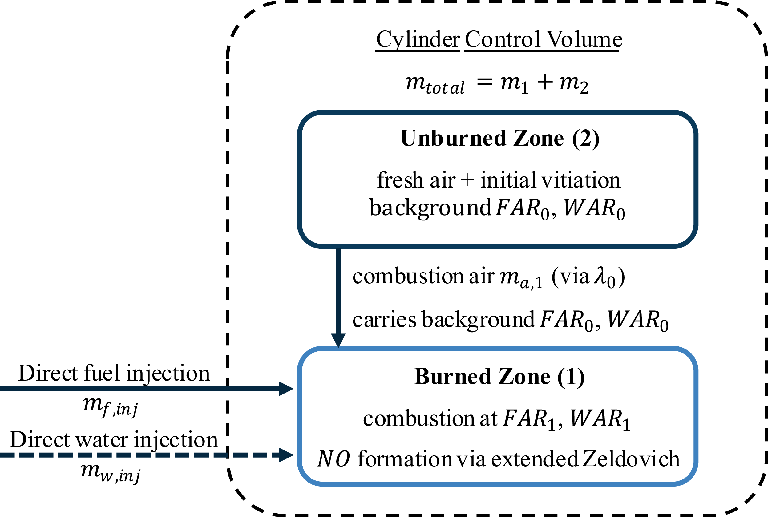

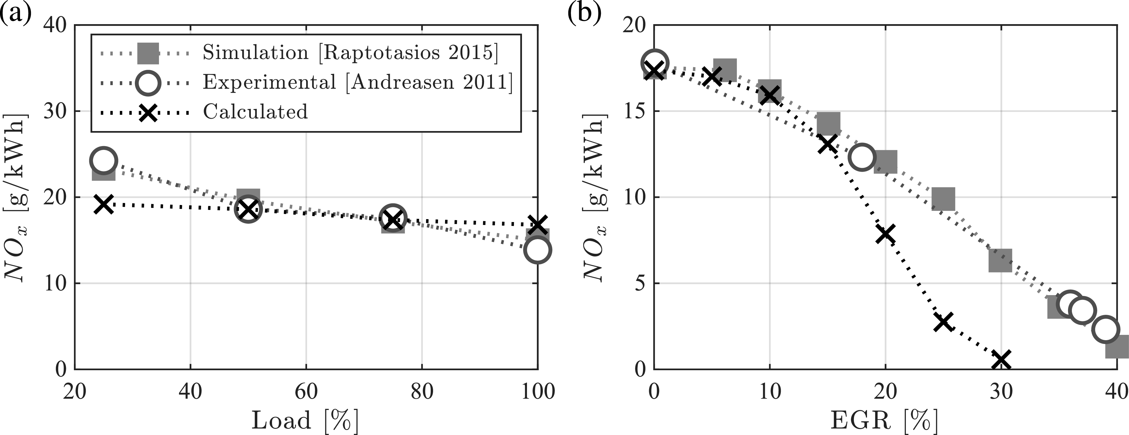
 NOx
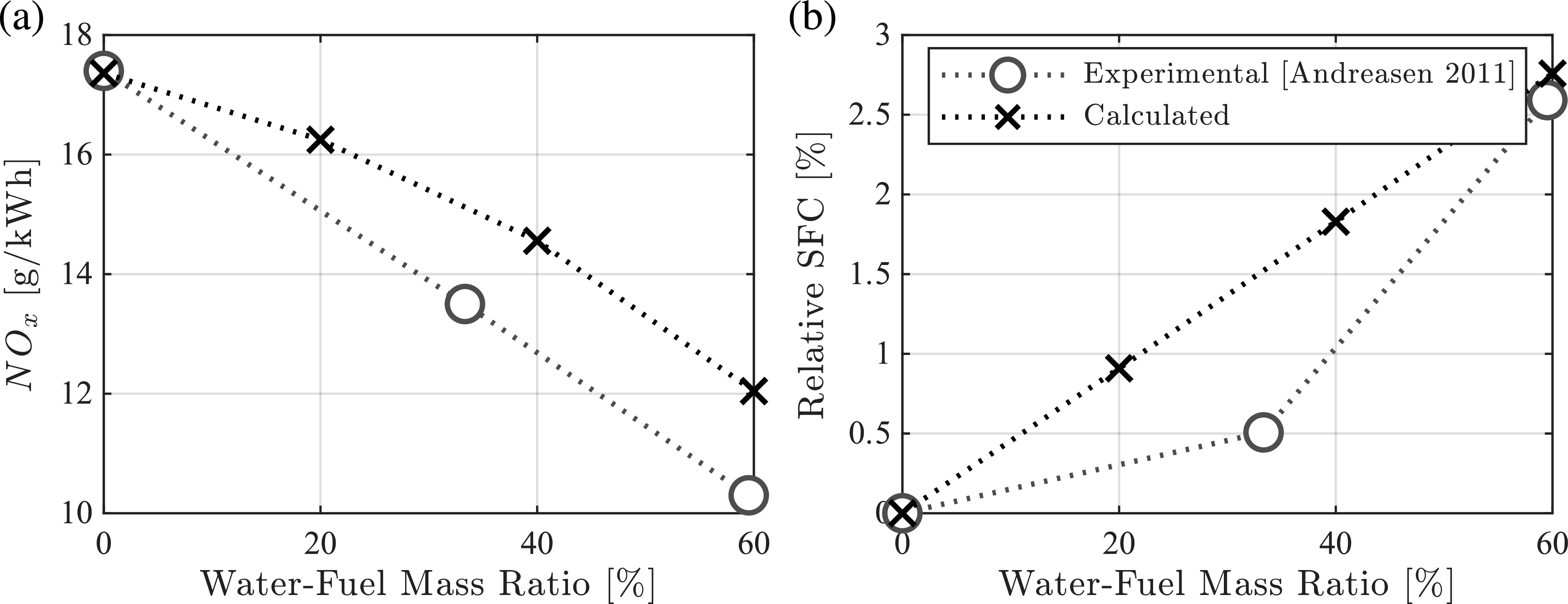
 NOx
 SFC
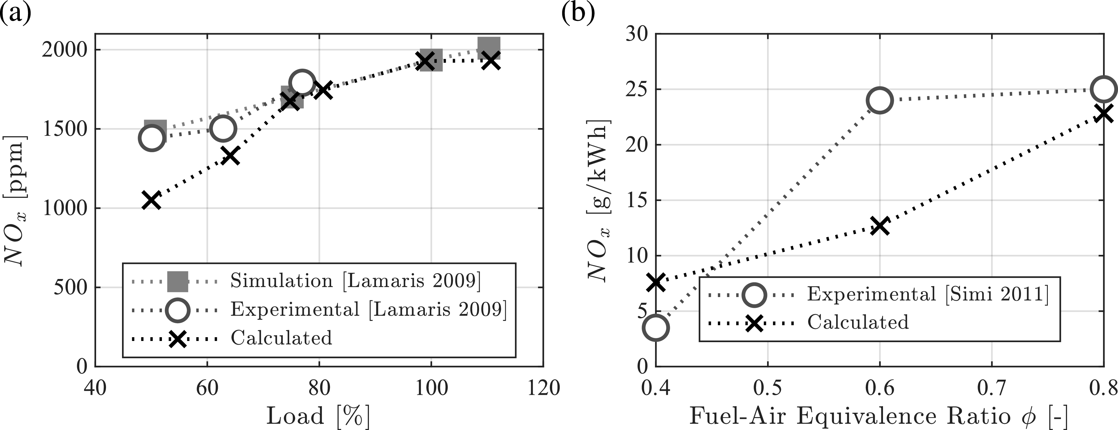
 NOx
 H2
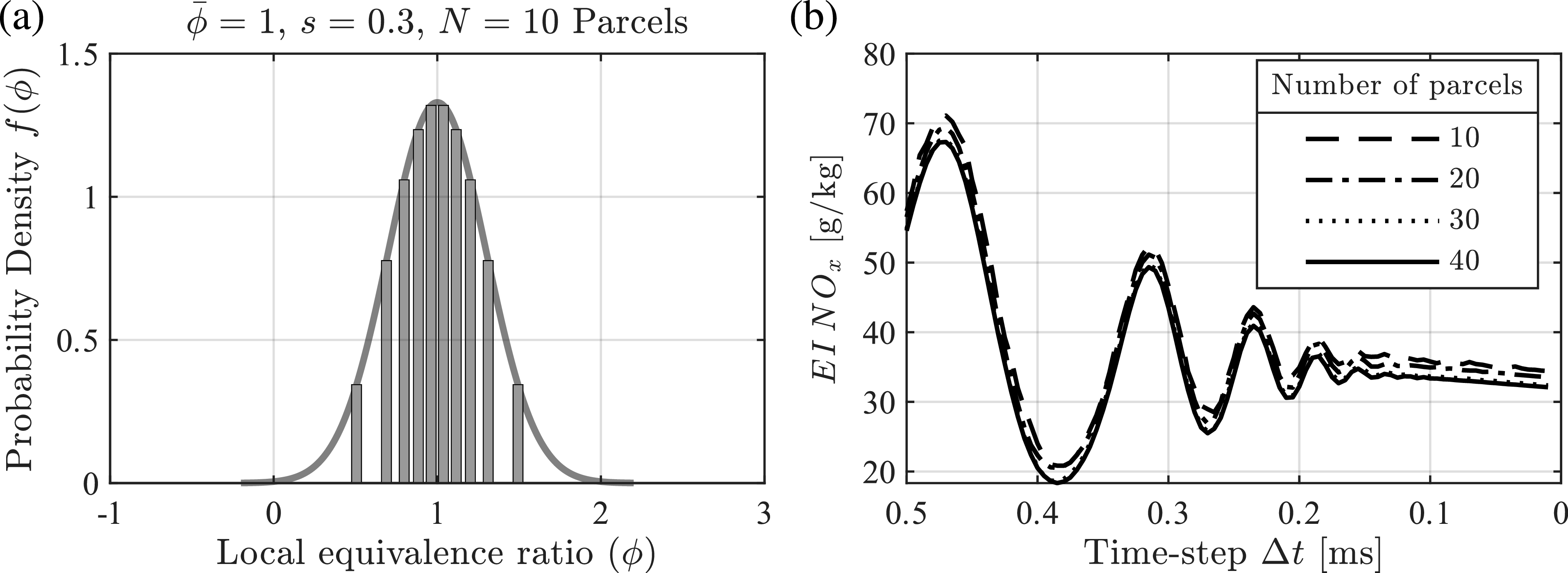
 NOx
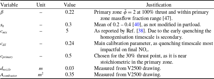
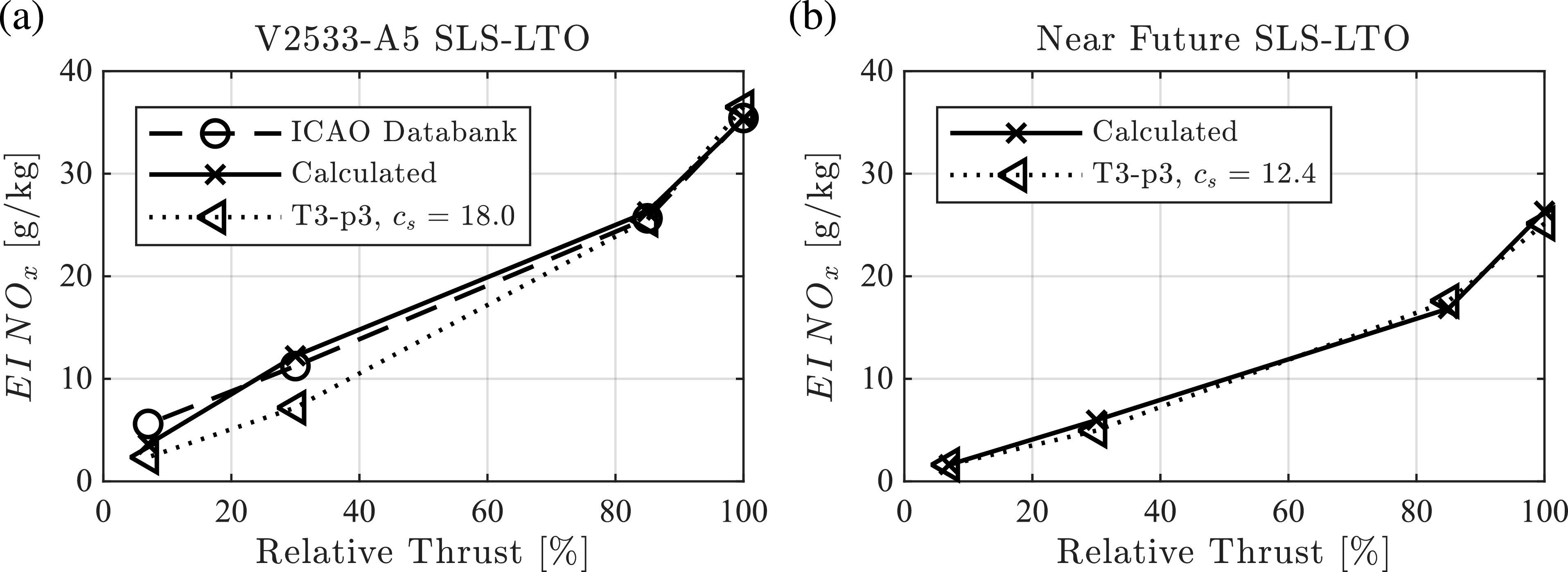
 NOx

 NOx
 30%
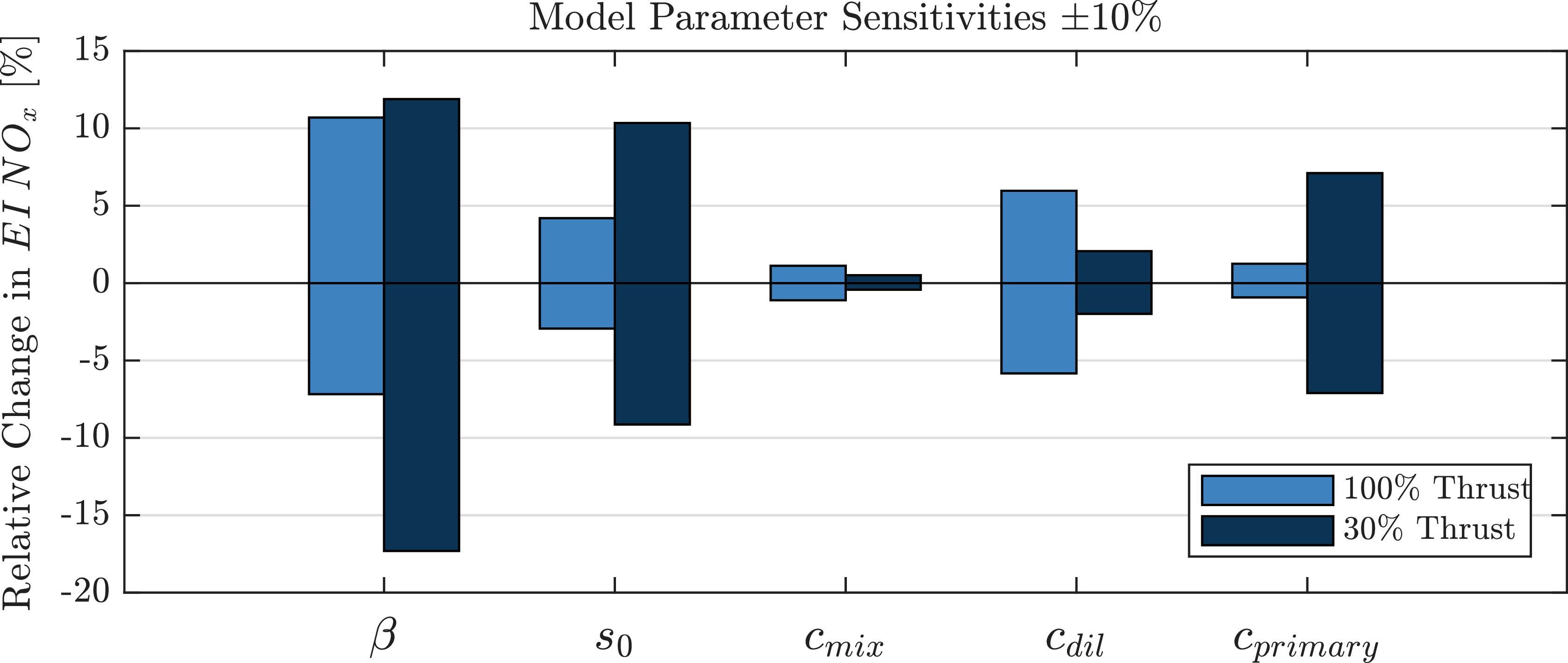
 NOx
 30

 NOx
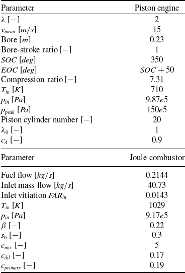

 NO

 λ

 Tinj=Tinlet=710K

 WFR
 Tinj
 wwater

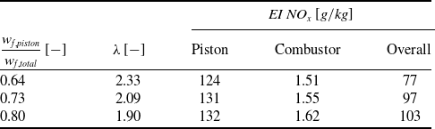
 NOx

 NO

 Open access

