1 Introduction
Thin liquid films are omnipresent in daily life and industry. Examples abound in coating flows (Weinstein & Ruschak Reference Weinstein and Ruschak2004), microfluidic devices (Ajaev & Homsy Reference Ajaev and Homsy2006), foam stability (Cohen-Addad, Höhler & Pitois Reference Cohen-Addad, Höhler and Pitois2013) and drop coalescence (Yoon et al. Reference Yoon, Baldessari, Ceniceros and Leal2007). Understanding the dynamics of thin film rupture is central to many of these applications. For example, the formation of dry spots in cooling systems relying on thin film flows driven by shear (Kabov Reference Kabov2000) can lead to loss of heat transfer efficiency. Premature rupture of the tear film in the eye can lead to dry-eye syndrome (Braun Reference Braun2012), a medical condition. The drainage of liquid films between gas bubbles and mineral particles is an important step in froth flotation (Nguyen & Schulze Reference Nguyen and Schulze2003).
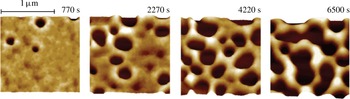
Temporal series of AFM scans recorded experimentally showing rupture of a 3.9 nm PS film on an oxidized Si wafer. For this system, the values of the Hamaker constant, surface tension and viscosity are
 $2.2\times 10^{-20}~\text{J}$
,
 $30.8~\text{mN}~\text{m}^{-1}$
and
 $12\,000~\text{Pa}~\text{s}$
. The scale bar that is shown above the leftmost image applies to all four images. Adapted by permission from Macmillan Publishers Ltd: Nature Materials (Becker et al.
Reference Becker, Grün, Seemann, Mantz, Jacobs, Mecke and Blossey2003), copyright 2003.

In many of the aforementioned examples, the thickness of the film is of the order of or less than a micrometre and, therefore, long-range intermolecular forces become significant in deciding the fate of the film and its stability (De Gennes Reference De Gennes1985; Kheshgi & Scriven Reference Kheshgi and Scriven1991; Reiter et al. Reference Reiter, Sharma, Casoli, David, Khanna and Auroy1999). The dewetting of a solid surface by film thinning and rupture has been termed spinodal dewetting (Mitlin Reference Mitlin1993) and has been observed experimentally (Reiter Reference Reiter1992; Stange, Evans & Hendrickson Reference Stange, Evans and Hendrickson1997; Becker et al. Reference Becker, Grün, Seemann, Mantz, Jacobs, Mecke and Blossey2003), as shown by the atomic force microscope (AFM) scans of figure 1 from Becker et al. (Reference Becker, Grün, Seemann, Mantz, Jacobs, Mecke and Blossey2003) that depict the rupture of a polystyrene (PS) film on a silicon (Si) wafer. Contributions to the free energy of the thin film due to intermolecular interactions lead to the addition of a disjoining pressure term (Teletzke, Davis & Scriven Reference Teletzke, Davis and Scriven1987) to the fluid pressure.
Consider a liquid film of uniform thickness
 $h_{0}$
that completely wets the solid substrate on which it is lying and that is surrounded by a dynamically passive gas such as air. Next consider that the film’s surface or the liquid–gas interface is perturbed so that the equation of the film’s surface is given by
 $\tilde{z}=\tilde{h}(\tilde{\boldsymbol{x}}_{H})$
, with the
 $\tilde{z}$
coordinate measured in the direction perpendicular to the solid,
 $\tilde{h}$
is the local film thickness and
 $\tilde{\boldsymbol{x}}_{H}=\tilde{\boldsymbol{x}}-\tilde{z}\boldsymbol{e}_{z}$
is the two-dimensional position vector that lies in the plane of the solid, with
 $\tilde{\boldsymbol{x}}$
and
 $\boldsymbol{e}_{z}$
standing for the position vector and the unit vector in the
 $\tilde{z}$
-direction. The pressure
 $\tilde{p}$
within a slightly perturbed film is then given by
 $$\begin{eqnarray}\tilde{p}=\frac{A}{6\unicode[STIX]{x03C0}\tilde{h}^{3}}-\unicode[STIX]{x1D70E}\tilde{\unicode[STIX]{x1D6FB}}_{H}^{2}\tilde{h}.\end{eqnarray}$$
Here, the effect of gravity is neglected on account of the film’s thinness, the pressure datum is taken to be that of the surrounding air,
 $A$
is the Hamaker constant,
 $\unicode[STIX]{x1D70E}$
is the surface tension and
 $\tilde{\unicode[STIX]{x1D735}}_{H}$
is the two-dimensional gradient operator given by
 $\tilde{\unicode[STIX]{x1D735}}_{H}\equiv \tilde{\unicode[STIX]{x1D735}}-\boldsymbol{e}_{z}(\unicode[STIX]{x2202}/\unicode[STIX]{x2202}\tilde{z})$
, with
 $\tilde{\unicode[STIX]{x1D735}}$
standing for the usual gradient operator. Equation (1.1) makes plain that there are two competing effects in a deformed film: the first term, which corresponds to the van der Waals pressure, is destabilizing because it would cause flow from the troughs, or valleys, to the crests, or hills, and lead to further localized thinning of the film whereas the second term, which corresponds to the capillary or surface tension pressure, is stabilizing, because it would cause flow from the crests to the troughs and lead to healing of the film. Ruckenstein & Jain (Reference Ruckenstein and Jain1974) developed a dynamic linear stability theory for an isothermal film on a horizontal plate based on the Navier–Stokes equations in the lubrication or long-wavelength limit modified by the addition of a body force term to account for intermolecular van der Waals attractions. These authors thereby showed that perturbations or disturbances of wavelengths exceeding a critical value
 $\tilde{\unicode[STIX]{x1D706}}_{c}$
are unstable where
 $$\begin{eqnarray}\tilde{\unicode[STIX]{x1D706}}_{c}=\left(\frac{8\unicode[STIX]{x03C0}^{3}\unicode[STIX]{x1D70E}}{A}\right)^{1/2}{h_{0}}^{2}=2\unicode[STIX]{x03C0}\frac{h_{0}}{d}h_{0},\end{eqnarray}$$
where
 $d\equiv (A/2\unicode[STIX]{x03C0}\unicode[STIX]{x1D70E})^{1/2}$
is the molecular length scale. For the continuum approximation to be valid,
 $h_{0}\gg d$
, which implies that the critical wavelength is much larger than the film thickness which justified their use of the lubrication approximation. These authors also calculated an estimate of the rupture time.
More recently, Williams & Davis (Reference Williams and Davis1982) used long-wave theory to derive a nonlinear evolution equation for the thickness of a film of a Newtonian fluid as a function of the lateral space coordinate
 $\tilde{x}$
and time
 $\tilde{t}$
. These authors reported that the rupture process is accelerated due to the nonlinear terms, thereby leading to rupture times much shorter than those predicted by linear theory. Zhang & Lister (Reference Zhang and Lister1999) solved this equation analytically and numerically to show that the lateral length scale
 $\tilde{x}^{\prime }\equiv \tilde{x}-\tilde{x}_{R}$
and film thickness vary with time remaining until rupture
 $\tilde{\unicode[STIX]{x1D70F}}\equiv \tilde{t}_{R}-\tilde{t}$
, where
 $(\tilde{x}_{R},\tilde{t}_{R})$
give the location of the space–time singularity where the film ruptures, as
 $\tilde{x}^{\prime }\sim \tilde{\unicode[STIX]{x1D70F}}^{2/5}$
and
 $\tilde{h}\sim \tilde{\unicode[STIX]{x1D70F}}^{1/5}$
, respectively, where
 $2/5$
and
 $1/5$
are the scaling exponents, for both line and point rupture. These authors thereby demonstrated that during the rupture of Newtonian films, the dominant force balance is between van der Waals, viscous and capillary forces. Since the relevant length and time scales in the vicinity of the rupture singularity are orders of magnitude smaller than similar variables in the far field, the dynamics in the vicinity of the rupture singularity is self-similar (see, e.g. Barenblatt (Reference Barenblatt1996) who discusses that self-similarity arises in problems that lack a length scale and Eggers (Reference Eggers1993, Reference Eggers1997) on the closely related problem of capillary pinching of liquid jets). With the scaling exponents in hand, an ordinary differential equation can then be derived for the self-similar film profile in similarity space. Zhang & Lister (Reference Zhang and Lister1999) demonstrated that transient solutions for the film profile and certain other quantities obtained by solving the partial differential evolution equation can be collapsed onto self-similar profiles and are in excellent agreement with the self-similar profiles obtained by solving the aforementioned ordinary differential equation in similarity space.
While the studies discussed in the previous two paragraphs were concerned with Newtonian fluids, many fluids in industrial and everyday applications are non-Newtonian in nature. An important type of a non-Newtonian fluid is the so-called power-law fluid. It derives its name from the power-law dependence (Deen Reference Deen1998) of the viscosity
 $\tilde{\unicode[STIX]{x1D707}}$
on the deformation rate
 $\tilde{\dot{\unicode[STIX]{x1D6FE}}}$
and is given by
 $$\begin{eqnarray}\tilde{\unicode[STIX]{x1D707}}(\tilde{\dot{\unicode[STIX]{x1D6FE}}})=\unicode[STIX]{x1D707}_{0}|2\tilde{m}\tilde{\dot{\unicode[STIX]{x1D6FE}}}|^{n-1}.\end{eqnarray}$$
Here,
 $\unicode[STIX]{x1D707}_{0}$
is the zero-deformation-rate viscosity of the fluid,
 $\tilde{m}^{-1}$
is the characteristic deformation rate,
 $n$
, where
 $0<n\leqslant 1$
, is the power-law exponent or index (
 $n=1$
corresponds to a Newtonian fluid) and
 $\tilde{\dot{\unicode[STIX]{x1D6FE}}}$
is the second invariant of the rate-of-deformation tensor
 $\tilde{\unicode[STIX]{x1D63F}}$
 $$\begin{eqnarray}\displaystyle & \displaystyle \tilde{\dot{\unicode[STIX]{x1D6FE}}}=\left[{\textstyle \frac{1}{2}}(\tilde{\unicode[STIX]{x1D63F}}\boldsymbol{ : }\tilde{\unicode[STIX]{x1D63F}})\right]^{1/2}, & \displaystyle\end{eqnarray}$$
 $$\begin{eqnarray}\displaystyle & \displaystyle \tilde{\unicode[STIX]{x1D63F}}={\textstyle \frac{1}{2}}[(\tilde{\unicode[STIX]{x1D735}}\tilde{\boldsymbol{v}})+(\tilde{\unicode[STIX]{x1D735}}\tilde{\boldsymbol{v}})^{\text{T}}], & \displaystyle\end{eqnarray}$$
where
 $\tilde{\boldsymbol{v}}$
is the fluid velocity. It has been shown experimentally that many fluids in industrial applications and in every day use exhibit power-law rheology (Bird et al.
Reference Bird, Armstrong, Hassager and Curtiss1977; Hasan, Ghannam & Esmail Reference Hasan, Ghannam and Esmail2010; Savage et al.
Reference Savage, Caggioni, Spicer and Cohen2010; Huisman, Friedman & Taborek Reference Huisman, Friedman and Taborek2012).
To date, extensive work has been done on the pinch-off singularity that arises during the breakup of threads or jets of power-law fluids. Scaling exponents and, in some cases, scaling functions or similarity profiles derived analytically (Renardy Reference Renardy2002; Doshi et al. Reference Doshi, Suryo, Yildirim, McKinley and Basaran2003; Doshi & Basaran Reference Doshi and Basaran2004) have been verified by comparison against numerical simulations (Doshi et al. Reference Doshi, Suryo, Yildirim, McKinley and Basaran2003; Doshi & Basaran Reference Doshi and Basaran2004; Suryo & Basaran Reference Suryo and Basaran2006) and experiments (Savage et al. Reference Savage, Caggioni, Spicer and Cohen2010; Huisman et al. Reference Huisman, Friedman and Taborek2012). Previous works on thin films of power-law fluids on a substrate have dealt with the dynamics of films flowing down inclined planes (Miladinova, Lebon & Toshev Reference Miladinova, Lebon and Toshev2004), falling films (Dandapat & Mukhopadhyay Reference Dandapat and Mukhopadhyay2003), films on cylinders (Gorla Reference Gorla2001), films on rotating discs (Arora & Doshi Reference Arora and Doshi2016) and tear films (Zhang, Matar & Craster Reference Zhang, Matar and Craster2003), albeit without delving into the self-similar dynamics that arises during film rupture. Moreover, while the study of the dynamics of rupture of thin free films or sheets of Newtonian fluids by Vaynblat, Lister & Witelski (Reference Vaynblat, Lister and Witelski2001) has recently been extended to power-law fluids by Thete et al. (Reference Thete, Anthony, Basaran and Doshi2015), studies have not been carried out to extend the pioneering study of Zhang & Lister (Reference Zhang and Lister1999) on rupture of supported films of Newtonian fluids to films of non-Newtonian fluids exhibiting power-law rheology. Filling this gap in knowledge on the rupture of supported films is the main goal of this work.
The organization of the paper is as follows. Section 2 describes in detail the problem under investigation and summarizes succinctly the equations and boundary conditions governing film thinning. Section 3 presents a derivation of the governing equations in the lubrication limit. Section 4 then derives and presents the nonlinear evolution equation for the transient film profile for the case of two-dimensional or line rupture and analyses theoretically and computationally the rupture of a thin film of a power-law fluid. Section 5 provides a treatment that mirrors that of the previous section albeit for situations in which a film undergoes axisymmetric or point rupture. Section 6 determines the conditions for which inertia becomes important and the lubrication approximation is no longer valid during thinning of power-law films. Section 7 summarizes the mathematical formulation of the problem for solving the equations governing film thinning without invoking the lubrication approximation and when inertia is important. This section presents the scaling exponents for the variation with time remaining until rupture of the film thickness, the lateral length scale and the lateral velocity that are expected in a thinning regime where inertia is important. In this section, the numerical method that is used to solve the transient, spatially two-dimensional set of partial differential equations comprised of the continuity and Cauchy momentum equations is also presented. In § 8, solutions obtained by solving the fully two-dimensional set of the aforementioned partial differential equations are presented and a transition from an initial thinning regime in which inertia is negligible to a final regime in which inertia is important is demonstrated. Section 9 concludes the paper by summarizing the key results that have been presented and outlines some possible future avenues for extending the analyses carried out in this work.
2 Problem statement
The system is an isothermal thin film of an incompressible power-law liquid of constant density
 $\unicode[STIX]{x1D70C}$
, non-constant viscosity
 $\tilde{\unicode[STIX]{x1D707}}$
and constant Hamaker constant
 $A$
. The film is initially quiescent and of uniform thickness
 $h_{0}$
. The film overlays or sits on top of a homogeneous solid substrate. The liquid–solid surface of contact is taken to coincide with the
 $\tilde{x}{\tilde{y}}$
-plane of a Cartesian coordinate system
 $(\tilde{x},{\tilde{y}},\tilde{z})$
or the
 $\tilde{r}\unicode[STIX]{x1D703}$
-plane of a cylindrical polar coordinate system
 $(\tilde{r},\unicode[STIX]{x1D703},\tilde{z})$
with its origin located on that surface and with the
 $\tilde{z}$
coordinate measured in the direction perpendicular to the solid. The region above the film is occupied by a dynamically passive gas, e.g. air, that exerts a constant pressure, set equal to zero w.l.o.g., on the film. The surface tension of the liquid–gas interface
 $\unicode[STIX]{x1D70E}$
is spatially uniform and constant.
The flow within the film is governed by the continuity and Cauchy momentum equations
 $$\begin{eqnarray}\displaystyle & \displaystyle \tilde{\unicode[STIX]{x1D735}}\boldsymbol{\cdot }\tilde{\boldsymbol{v}}=0, & \displaystyle\end{eqnarray}$$
 $$\begin{eqnarray}\displaystyle & \displaystyle \unicode[STIX]{x1D70C}\left(\frac{\unicode[STIX]{x2202}\tilde{\boldsymbol{v}}}{\unicode[STIX]{x2202}\tilde{t}}+\tilde{\boldsymbol{v}}\boldsymbol{\cdot }\tilde{\unicode[STIX]{x1D735}}\tilde{\boldsymbol{v}}\right)=\tilde{\unicode[STIX]{x1D735}}\boldsymbol{\cdot }\tilde{\unicode[STIX]{x1D64F}}. & \displaystyle\end{eqnarray}$$
Here,
 $\tilde{\boldsymbol{v}}$
is the velocity,
 $\tilde{t}$
is time and
 $\tilde{\unicode[STIX]{x1D64F}}=-\tilde{p}\unicode[STIX]{x1D644}+\tilde{\unicode[STIX]{x1D749}}$
is the stress tensor with
 $\tilde{p}$
the pressure and
 $\tilde{\unicode[STIX]{x1D749}}$
the viscous stress tensor. For a power-law liquid,
 $\tilde{\unicode[STIX]{x1D749}}=2\tilde{\unicode[STIX]{x1D707}}\tilde{\unicode[STIX]{x1D63F}}$
. In (2.2) and the remainder of the paper, the effect of gravity on the dynamics is also taken to be negligible on account of the film’s thinness.
Along the solid surface bounding the liquid film (
 $\tilde{z}=0$
), the liquid must obey no slip and no penetration or the adherence boundary condition
 $$\begin{eqnarray}\tilde{\boldsymbol{v}}=\mathbf{0}.\end{eqnarray}$$
At the liquid–gas interface, the kinematic and traction boundary conditions are applied to enforce no mass transfer across the free surface
 $S(\tilde{t})$
and the jump in the traction vector due to surface tension and van der Waals forces:
 $$\begin{eqnarray}\displaystyle & \displaystyle \boldsymbol{n}\boldsymbol{\cdot }(\tilde{\boldsymbol{v}}-\tilde{\boldsymbol{v}}_{s})=0, & \displaystyle\end{eqnarray}$$
 $$\begin{eqnarray}\displaystyle & \displaystyle \boldsymbol{n}\boldsymbol{\cdot }\tilde{\unicode[STIX]{x1D64F}}=2\tilde{H}\unicode[STIX]{x1D70E}\boldsymbol{n}-\frac{A}{6\unicode[STIX]{x03C0}\tilde{h}^{3}}\boldsymbol{n}. & \displaystyle\end{eqnarray}$$
Here,
 $\tilde{\boldsymbol{v}}_{s}$
is the velocity of points on the interface
 $S(\tilde{t})$
,
 $\boldsymbol{n}$
is the unit normal vector to
 $S(\tilde{t})$
and
 $2\tilde{H}$
is twice the mean curvature of
 $S(\tilde{t})$
.
In addition to the boundary conditions that have been imposed in the vertical direction, i.e. along the free surface
 $S(\tilde{t})$
and the solid substrate (
 $\tilde{z}=0$
), boundary conditions also need to be specified in the lateral direction. The latter are presented in the following sections when different rupture scenarios are analysed. The mathematical statement of the problem is completed by the specification of initial conditions. These too are provided in subsequent sections where the lateral boundary conditions are specified.
3 Film rupture in the lubrication limit
As the disturbances that cause the film to destabilize are of long wavelengths
 $\tilde{\unicode[STIX]{x1D706}}$
, advantage will be taken in this section of the fact that
 $\unicode[STIX]{x1D716}\equiv h_{0}/l_{c}\ll 1$
, where
 $l_{c}=O(\tilde{\unicode[STIX]{x1D706}})$
is the lateral or horizontal length scale, to simplify the governing Cauchy momentum and continuity equations by invoking the lubrication approximation (Deen Reference Deen1998; Leal Reference Leal2007). The details of the simplification of the governing equations and the derivation of the lubrication equations are presented in appendix A.
The equations governing the flow within the film in dimensional form are then given by
 $$\begin{eqnarray}\displaystyle & \displaystyle -\tilde{\unicode[STIX]{x1D735}}_{H}\tilde{p}+\frac{\unicode[STIX]{x2202}}{\unicode[STIX]{x2202}\tilde{z}}\left(\tilde{\unicode[STIX]{x1D707}}\frac{\unicode[STIX]{x2202}\tilde{\boldsymbol{v}}_{H}}{\unicode[STIX]{x2202}\tilde{z}}\right)=0, & \displaystyle\end{eqnarray}$$
 $$\begin{eqnarray}\displaystyle & \displaystyle \frac{\unicode[STIX]{x2202}\tilde{p}}{\unicode[STIX]{x2202}\tilde{z}}=0, & \displaystyle\end{eqnarray}$$
 $$\begin{eqnarray}\displaystyle & \displaystyle \frac{\unicode[STIX]{x2202}\tilde{h}}{\unicode[STIX]{x2202}\tilde{t}}+\tilde{\unicode[STIX]{x1D735}}_{H}\boldsymbol{\cdot }\int _{0}^{\tilde{h}}\boldsymbol{v}_{H}\,\text{d}\tilde{z}=0, & \displaystyle\end{eqnarray}$$
where
 $\tilde{\boldsymbol{v}}_{H}\equiv \tilde{\boldsymbol{v}}-\tilde{w}\boldsymbol{e}_{z}$
is the velocity parallel to the substrate and
 $\tilde{w}$
is the component of the velocity in the direction normal to it. As shown in appendix A, equations (3.1) and (3.2) follow from the horizontal and vertical components of the Cauchy momentum equation after invoking the lubrication approximation. It can be readily shown that in thin film flow,
 $\tilde{\dot{\unicode[STIX]{x1D6FE}}}^{2}=((\unicode[STIX]{x2202}\tilde{\boldsymbol{v}}_{H}/\unicode[STIX]{x2202}\tilde{z})\cdot (\unicode[STIX]{x2202}\tilde{\boldsymbol{v}}_{H}/\unicode[STIX]{x2202}\tilde{z}))/4$
so that the viscosity of the film fluid is given by
 $$\begin{eqnarray}\tilde{\unicode[STIX]{x1D707}}(\tilde{\dot{\unicode[STIX]{x1D6FE}}})=\unicode[STIX]{x1D707}_{0}\left|\tilde{m}\left(\frac{\unicode[STIX]{x2202}\tilde{\boldsymbol{v}}_{H}}{\unicode[STIX]{x2202}\tilde{z}}\cdot \frac{\unicode[STIX]{x2202}\tilde{\boldsymbol{v}}_{H}}{\unicode[STIX]{x2202}\tilde{z}}\right)^{1/2}\right|^{n-1}.\end{eqnarray}$$
Equation (3.3) results when the continuity equation is integrated across the film thickness and is then combined with the kinematic boundary condition at the liquid–gas interface. In these equations and below,
 $\tilde{z}=\tilde{h}(\tilde{\boldsymbol{x}}_{H},\tilde{t})$
gives the location of the liquid–gas interface where
 $\tilde{h}$
is the instantaneous value of the local film thickness. As is the case with all lubrication flows, equation (3.2) shows that the pressure does not vary across the film and when this result is combined with the normal component of the traction boundary condition at the film’s surface, it follows that the pressure within the film is given by (1.1).
Equations (3.1)–(3.3) are solved subject to the following boundary conditions:
 $$\begin{eqnarray}\displaystyle & \displaystyle \tilde{\boldsymbol{v}}_{H}=\mathbf{0}\quad \text{at }\tilde{z}=0, & \displaystyle\end{eqnarray}$$
 $$\begin{eqnarray}\displaystyle & \displaystyle \frac{\unicode[STIX]{x2202}\tilde{\boldsymbol{v}}_{H}}{\unicode[STIX]{x2202}\tilde{z}}=\mathbf{0}\quad \text{at }\tilde{z}=\tilde{h}. & \displaystyle\end{eqnarray}$$
Equation (3.5) is the usual no-slip boundary condition on the substrate and the free-slip condition at the film’s surface in (3.6) follows from the tangential component of the traction boundary condition in the lubrication limit.
Before solving the equations governing film thinning and rupture, it is advantageous to non-dimensionalize the problem variables. This is accomplished by introducing the following characteristic scales for film thickness
 $h_{c}$
, lateral length
 $l_{c}$
, time
 $t_{c}$
, pressure
 $p_{c}$
and lateral velocity
 $u_{c}$
 $$\begin{eqnarray}\displaystyle & \displaystyle h_{c}\equiv h_{0}, & \displaystyle\end{eqnarray}$$
 $$\begin{eqnarray}\displaystyle & \displaystyle l_{c}\equiv \frac{h_{0}^{2}}{d}=\frac{\tilde{\unicode[STIX]{x1D706}}_{c}}{2\unicode[STIX]{x03C0}}, & \displaystyle\end{eqnarray}$$
 $$\begin{eqnarray}\displaystyle & \displaystyle t_{c}\equiv \frac{12\unicode[STIX]{x03C0}^{2}\unicode[STIX]{x1D707}_{0}\unicode[STIX]{x1D70E}{h_{0}}^{5}}{A^{2}}=3\left(\frac{\unicode[STIX]{x1D707}_{0}h_{0}}{\unicode[STIX]{x1D70E}}\right)\left(\frac{h_{0}}{d}\right)^{4}, & \displaystyle\end{eqnarray}$$
 $$\begin{eqnarray}\displaystyle & \displaystyle p_{c}\equiv \frac{A}{6\unicode[STIX]{x03C0}h_{0}^{3}}=\frac{\unicode[STIX]{x1D70E}h_{0}}{3l_{c}^{2}}, & \displaystyle\end{eqnarray}$$
 $$\begin{eqnarray}\displaystyle & \displaystyle u_{c}\equiv \frac{l_{c}}{t_{c}}=\frac{1}{3}\left(\frac{\unicode[STIX]{x1D70E}}{\unicode[STIX]{x1D707}_{0}}\right)\left(\frac{d}{h_{0}}\right)^{3}. & \displaystyle\end{eqnarray}$$
With these scales, the dimensionless variables are then given by:
 $$\begin{eqnarray}h\equiv \frac{\tilde{h}}{h_{0}},\quad z\equiv \frac{\tilde{z}}{h_{0}},\quad t\equiv \frac{\tilde{t}}{t_{c}},\end{eqnarray}$$
 $$\begin{eqnarray}\boldsymbol{x}_{H}\equiv \frac{\tilde{\boldsymbol{x}}_{H}}{l_{c}},\quad \unicode[STIX]{x1D735}_{H}\equiv l_{c}\tilde{\unicode[STIX]{x1D735}}_{H},\quad \unicode[STIX]{x1D706}\equiv \frac{\tilde{\unicode[STIX]{x1D706}}}{l_{c}},\end{eqnarray}$$
 $$\begin{eqnarray}p\equiv \frac{\tilde{p}}{p_{c}},\quad \boldsymbol{v}_{H}\equiv \frac{\tilde{\boldsymbol{v}}_{H}}{u_{c}},\end{eqnarray}$$
 $$\begin{eqnarray}\unicode[STIX]{x1D707}\equiv \frac{\tilde{\unicode[STIX]{x1D707}}}{\unicode[STIX]{x1D707}_{0}},\quad m\equiv \tilde{m}\frac{u_{c}}{h_{0}}.\end{eqnarray}$$
In (3.12)–(3.15), variables without tildes over them are the dimensionless counterparts of those with tildes.
In the following two sections, the governing equations (3.1)–(3.3), subject to the boundary conditions (3.5)–(3.6), written in dimensionless form will be solved first for the case of line rupture or when the rupture is two-dimensional and then for the case of point rupture or when the rupture is axisymmetric. In both cases, the initial conditions will entail subjecting a quiescent flat film to a periodic shape perturbation having a wavelength exceeding
 $\unicode[STIX]{x1D706}_{c}\equiv \tilde{\unicode[STIX]{x1D706}}_{c}/l_{c}=2\unicode[STIX]{x03C0}$
and following the thinning of the film until rupture.
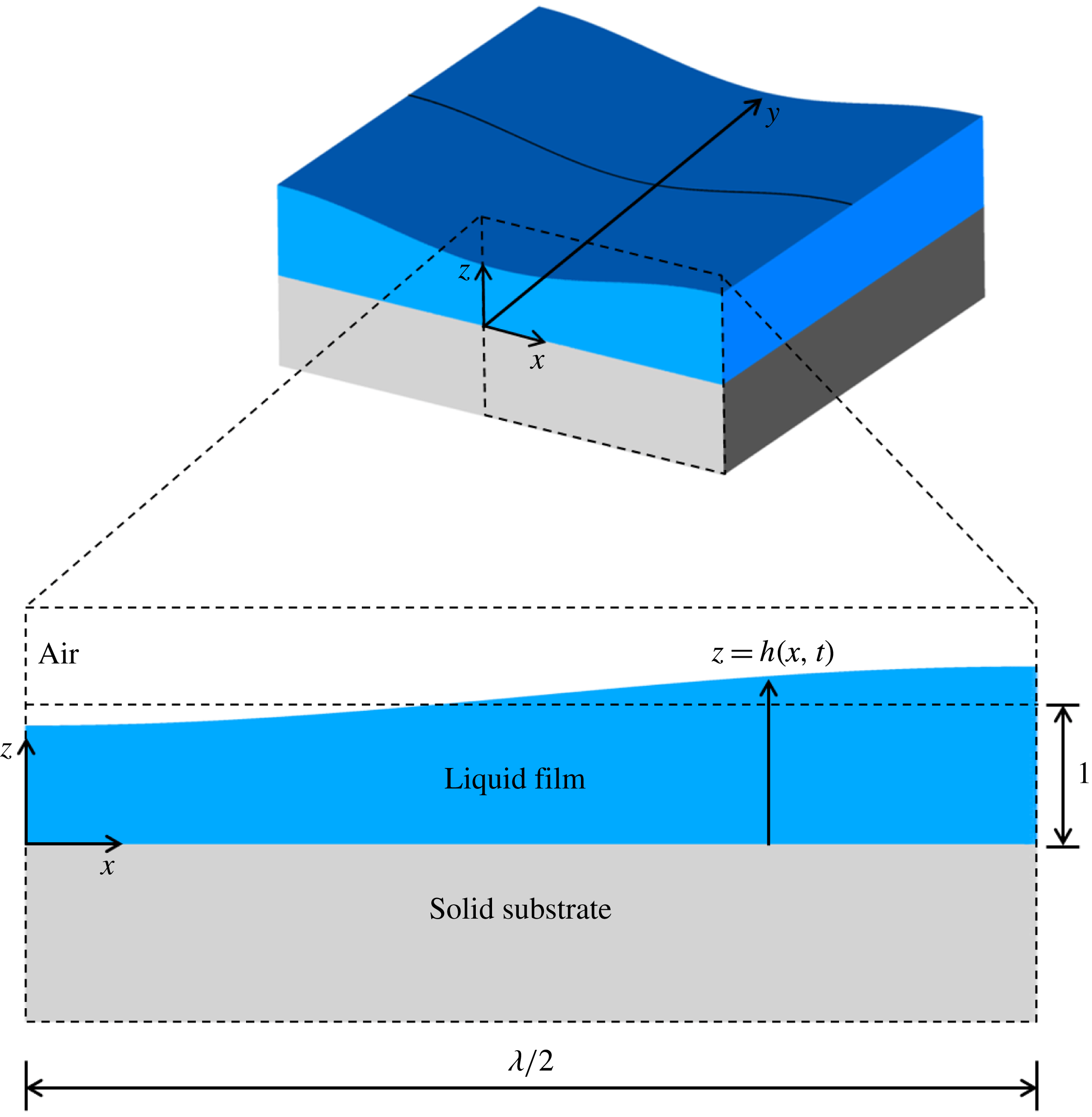
Line rupture. Top: perspective view of a film on a substrate showing the deformed interface over a lateral extent corresponding to one wavelength
 $\unicode[STIX]{x1D706}$
of the imposed perturbation. Bottom: a blow-up or zoomed-in cross-sectional view of the film over a lateral extent corresponding to a half of a wavelength of the imposed perturbation. Because of symmetry, the problem domain is
 $0\leqslant x\leqslant \unicode[STIX]{x1D706}/2$
.

4 Two-dimensional or line rupture in the lubrication limit
In this section, the initially flat surface of the film is subjected to a sinusoidal shape perturbation that is translationally symmetric or invariant in the
 $y$
-direction, where
 $y\equiv {\tilde{y}}/l_{c}$
, and has wavelength
 $\unicode[STIX]{x1D706}$
in the lateral or
 $x$
-direction, where
 $x\equiv \tilde{x}/l_{c}$
, as shown in figure 2. Since the perturbation is two-dimensional in nature, equation (3.1) subjected to boundary conditions (3.5) and (3.6) is solved in Cartesian coordinates such that
 $\boldsymbol{v}_{H}=u(x,z,t)\boldsymbol{e}_{x}$
and
 $\unicode[STIX]{x1D735}_{H}=\boldsymbol{e}_{x}(\unicode[STIX]{x2202}/\unicode[STIX]{x2202}x)$
, where
 $\boldsymbol{e}_{x}$
is a unit vector in the
 $x$
-direction, to arrive at the following expression for the dimensionless lateral velocity
 $u(x,z,t)$
 $$\begin{eqnarray}u(x,z,t)=\frac{n}{n+1}\frac{|\unicode[STIX]{x2202}p/\unicode[STIX]{x2202}x|}{\unicode[STIX]{x2202}p/\unicode[STIX]{x2202}x}m^{1/n-1}\left|\frac{\unicode[STIX]{x2202}p}{\unicode[STIX]{x2202}x}\right|^{1/n}\left[(h-z)^{1/n+1}-h^{1/n+1}\right],\end{eqnarray}$$
where
 $h(x,t)$
is the dimensionless local film thickness and
 $(|\unicode[STIX]{x2202}p/\unicode[STIX]{x2202}x|)/(\unicode[STIX]{x2202}p/\unicode[STIX]{x2202}x)$
denotes the sign of
 $\unicode[STIX]{x2202}p/\unicode[STIX]{x2202}x$
. In arriving at (4.1), use is made of the fact that in Cartesian coordinates, the dimensionless viscosity (cf. (3.4)) and the dimensionless fluid pressure
 $p(x,t)$
are given by
 $$\begin{eqnarray}\unicode[STIX]{x1D707}=\left|m\frac{\unicode[STIX]{x2202}u}{\unicode[STIX]{x2202}z}\right|^{n-1}\end{eqnarray}$$
and
 $$\begin{eqnarray}p(x,t)=\frac{1}{h^{3}}-3\frac{\unicode[STIX]{x2202}^{2}h}{\unicode[STIX]{x2202}x^{2}}.\end{eqnarray}$$
When the expression for
 $u$
given by (4.1) is substituted into (3.3), a spatially one-dimensional (1-D), nonlinear evolution equation results that governs the variation of the film thickness with the dimensionless lateral coordinate
 $x$
and dimensionless time
 $t$
 $$\begin{eqnarray}\frac{\unicode[STIX]{x2202}h}{\unicode[STIX]{x2202}t}-\frac{|\unicode[STIX]{x2202}p/\unicode[STIX]{x2202}x|}{\unicode[STIX]{x2202}p/\unicode[STIX]{x2202}x}m^{1/n-1}\frac{\unicode[STIX]{x2202}}{\unicode[STIX]{x2202}x}\left[\frac{n}{2n+1}\left|\frac{\unicode[STIX]{x2202}p}{\unicode[STIX]{x2202}x}\right|^{1/n}h^{1/n+2}\right]=0.\end{eqnarray}$$
Because of the periodic nature of the imposed perturbation, it is sufficient to solve the problem over the spatial domain spanning one half of the wavelength of the imposed perturbation, viz.
 $0\leqslant x\leqslant \unicode[STIX]{x1D706}/2$
, as shown in figure 2. Hence, the 1-D evolution equation is solved subject to the symmetry boundary conditions
 $$\begin{eqnarray}\frac{\unicode[STIX]{x2202}h}{\unicode[STIX]{x2202}x}=\frac{\unicode[STIX]{x2202}^{3}h}{\unicode[STIX]{x2202}x^{3}}=0\quad \text{at }x=0,\unicode[STIX]{x1D706}/2\end{eqnarray}$$
and initial condition
 $$\begin{eqnarray}h(x,0)=1-\unicode[STIX]{x1D6FF}\cos (2\unicode[STIX]{x03C0}x/\unicode[STIX]{x1D706}),\end{eqnarray}$$
where
 $\unicode[STIX]{x1D6FF}$
is the amplitude of the perturbation that is imposed to initiate the thinning of the film.
4.1 Scaling and self-similarity
The film profile is expected to be self-similar in the vicinity of the location where the film thickness is minimum as the rupture singularity
 $(x_{R},t_{R})$
is approached. Hence, by the similarity ansatz, the film profile in the vicinity of the rupture point should have the functional form
 $$\begin{eqnarray}h(x^{\prime },\unicode[STIX]{x1D70F})=\unicode[STIX]{x1D70F}^{\unicode[STIX]{x1D6FC}}H(\unicode[STIX]{x1D702}),\quad \unicode[STIX]{x1D702}=x^{\prime }/\unicode[STIX]{x1D70F}^{\unicode[STIX]{x1D6FD}},\end{eqnarray}$$
where
 $\unicode[STIX]{x1D70F}\equiv t_{R}-t$
is the dimensionless time remaining until rupture,
 $x^{\prime }\equiv x-x_{R}$
is the lateral extent of this rupture zone,
 $\unicode[STIX]{x1D702}$
is the similarity variable,
 $\unicode[STIX]{x1D6FC}$
and
 $\unicode[STIX]{x1D6FD}$
are the scaling exponents for
 $h$
and
 $x^{\prime }$
, respectively, and
 $H(\unicode[STIX]{x1D702})$
is the scaling function for the film profile in similarity space. Balancing the van der Waals (
 $vdW$
), surface tension or capillary (
 $ST$
) and viscous (
 $V$
) stresses in (3.1) and (4.2) and (4.3) shows that the scaling exponents
 $\unicode[STIX]{x1D6FC}$
and
 $\unicode[STIX]{x1D6FD}$
are given by
 $$\begin{eqnarray}\unicode[STIX]{x1D6FC}=\frac{n}{n+4},\quad \unicode[STIX]{x1D6FD}=\frac{2n}{n+4}.\end{eqnarray}$$
The scaling exponents given in (4.8) can also be obtained by substituting (4.7) into (4.4) and (4.3), and requiring that the resulting ordinary differential equation in similarity space be independent of time.
It readily follows from the dimensionless form of (3.1) and (4.2) and (4.3) that the van der Waals, surface tension or capillary and viscous stresses scale as
 $$\begin{eqnarray}\displaystyle & \displaystyle v\,dW\sim \left\Vert \frac{\unicode[STIX]{x2202}}{\unicode[STIX]{x2202}x}\left(\frac{1}{h^{3}}\right)\right\Vert \sim \frac{1}{x^{\prime }h^{3}}, & \displaystyle\end{eqnarray}$$
 $$\begin{eqnarray}\displaystyle & \displaystyle ST\sim \left\Vert \frac{\unicode[STIX]{x2202}}{\unicode[STIX]{x2202}x}\left(\frac{\unicode[STIX]{x2202}^{2}h}{\unicode[STIX]{x2202}x^{2}}\right)\right\Vert \sim \frac{h}{{x^{\prime }}^{3}}, & \displaystyle\end{eqnarray}$$
 $$\begin{eqnarray}\displaystyle & \displaystyle V\sim \left\Vert \frac{\unicode[STIX]{x2202}}{\unicode[STIX]{x2202}z}\left(\unicode[STIX]{x1D707}\frac{\unicode[STIX]{x2202}u}{\unicode[STIX]{x2202}z}\right)\right\Vert \sim \left\Vert \frac{\unicode[STIX]{x2202}}{\unicode[STIX]{x2202}z}\left(\frac{\unicode[STIX]{x2202}u}{\unicode[STIX]{x2202}z}\right)^{n}\right\Vert \sim \frac{u^{n}}{z^{n+1}}\sim \frac{(x^{\prime }/\unicode[STIX]{x1D70F})^{n}}{h^{n+1}}, & \displaystyle\end{eqnarray}$$
where
 $\Vert (\cdots )\Vert$
stands for the magnitude of the quantity ‘
 $(\cdots )$
’. Therefore, with the scaling exponents given by (4.8), all three stresses can be seen to scale as
 $\unicode[STIX]{x1D70F}\rightarrow 0$
as
 $$\begin{eqnarray}v\,dW\sim ST\sim V\sim \unicode[STIX]{x1D70F}^{-5n/(n+4)}.\end{eqnarray}$$
A noteworthy feature of the dynamics is that the scaling exponent for the lateral length scale
 $\unicode[STIX]{x1D6FD}$
is twice that for the vertical length scale (or film thickness)
 $\unicode[STIX]{x1D6FC}$
, viz.
 $\unicode[STIX]{x1D6FD}=2\unicode[STIX]{x1D6FC}$
. The reason for this relationship between the two scaling exponents follows from the balance between the van der Waals and surface tension stresses (cf. (4.9) and (4.10)). Initially, the lateral extent of the film is orders of magnitude larger than its thickness. As the film continues to thin and tends toward rupture, the rupture zone shrinks and hence both the lateral and vertical length scales in the vicinity of the point of rupture tend to zero. Therefore, given the initial disparity in the two length scales, it accords with intuition that the lateral length scale should tend to zero faster than the film thickness. For future reference, it is worth noting that fluid viscosity in the thinning film scales as
 $$\begin{eqnarray}\unicode[STIX]{x1D707}\sim \left\Vert \frac{\unicode[STIX]{x2202}u}{\unicode[STIX]{x2202}z}\right\Vert ^{n-1}\sim \frac{(x^{\prime }/\unicode[STIX]{x1D70F})^{n-1}}{z^{n-1}}\sim \unicode[STIX]{x1D70F}^{4(1-n)/(n+4)}.\end{eqnarray}$$
In concluding this subsection, it is also worth noting that in the Newtonian limit
 $(n=1)$
, the expressions in (4.8) for the scaling exponents take on the values of
 $\unicode[STIX]{x1D6FC}=1/5$
and
 $\unicode[STIX]{x1D6FD}=2/5$
and all three stresses diverge as
 $\unicode[STIX]{x1D70F}^{-1}$
(cf. (4.12)), in agreement with previous work on rupture of Newtonian films (Zhang & Lister Reference Zhang and Lister1999).
4.2 Simulation of line rupture in the lubrication limit
The spatially fourth-order nonlinear evolution equation (4.4) subject to boundary conditions (4.5) and initial condition (4.6) with
 $\unicode[STIX]{x1D6FF}=0.1$
is solved numerically using a Galerkin finite-element-based method to verify the scaling exponents that have just been determined and to demonstrate the self-similarity of the film profiles in the rupture zone. We have used variants of this algorithm to successfully solve 1-D long-wave evolution equations that arise in a variety of physical problems including dripping and jetting of Newtonian (Ambravaneswaran, Phillips & Basaran Reference Ambravaneswaran, Phillips and Basaran2000) as well as power-law fluids (Yildirim & Basaran Reference Yildirim and Basaran2006) from faucets, breakup of bridges of Newtonian (Zhang, Padgett & Basaran Reference Zhang, Padgett and Basaran1996) and power-law fluids (Yildirim & Basaran Reference Yildirim and Basaran2001) and rupture of sheets of Newtonian (Thete et al.
Reference Thete, Anthony, Doshi, Harris and Basaran2016) and power-law fluids (Thete et al.
Reference Thete, Anthony, Basaran and Doshi2015), among others. The simulation results to be reported have been obtained using a value of
 $\unicode[STIX]{x1D706}=4\unicode[STIX]{x03C0}$
. Use of larger values of the wavelength had no effect whatsoever on the values of the scaling exponents and the behaviour of the solutions in the vicinity of the point of rupture.
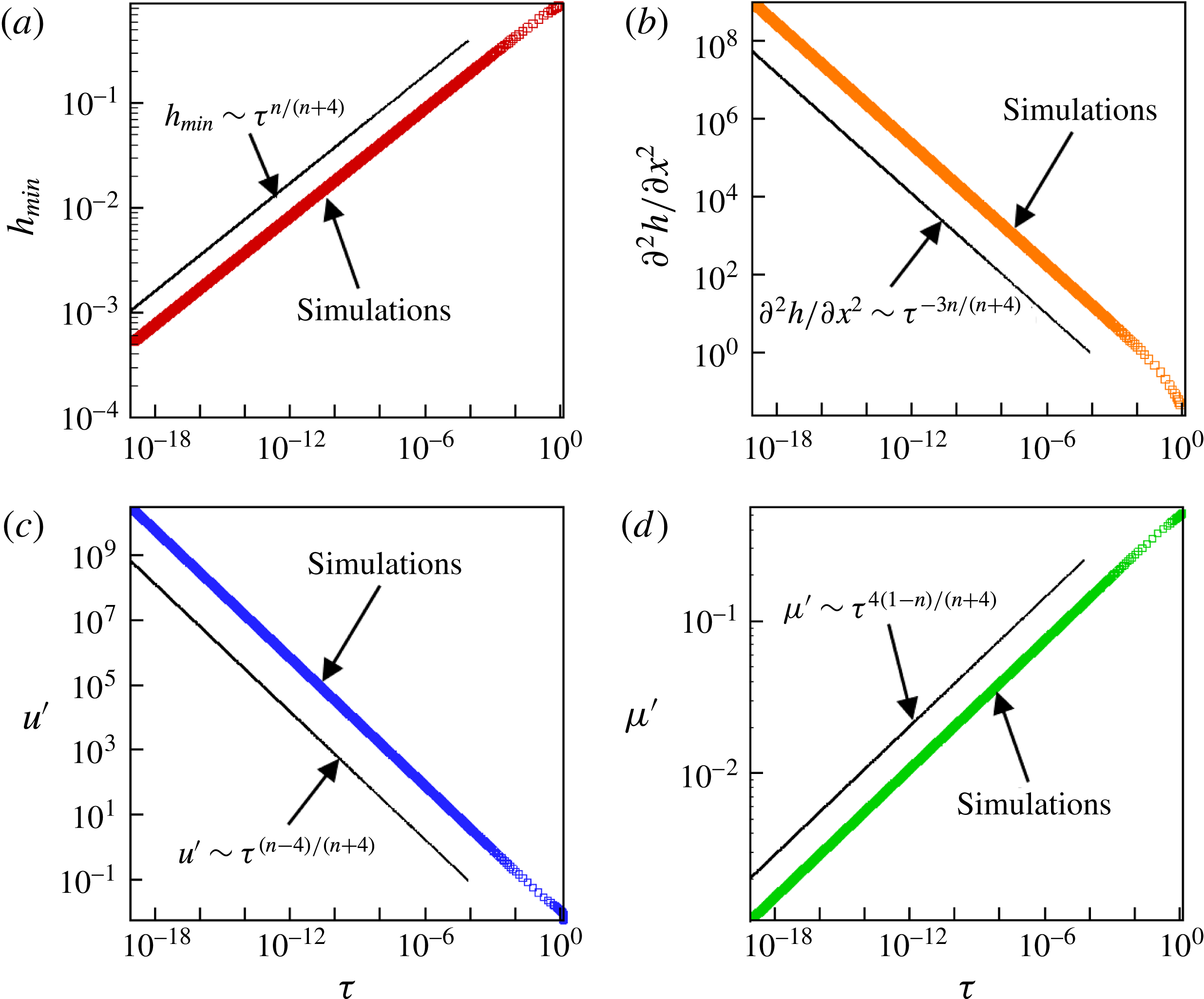
Scaling behaviour of variables in the rupture zone during thinning of a film of power-law index of
 $n=0.83$
undergoing line rupture: simulations (data points) and scaling theory predictions (straight lines with indicated dependencies on time remaining until rupture
 $\unicode[STIX]{x1D70F}$
). Variation with
 $\unicode[STIX]{x1D70F}$
of (a) minimum film thickness
 $h_{min}$
, (b) curvature
 $\unicode[STIX]{x2202}^{2}h/\unicode[STIX]{x2202}x^{2}$
evaluated at
 $x=0$
, (c) lateral velocity
 $u^{\prime }$
evaluated at lateral location where
 $h=1.001h_{min}$
and (d) viscosity
 $\unicode[STIX]{x1D707}^{\prime }$
evaluated at that lateral location.

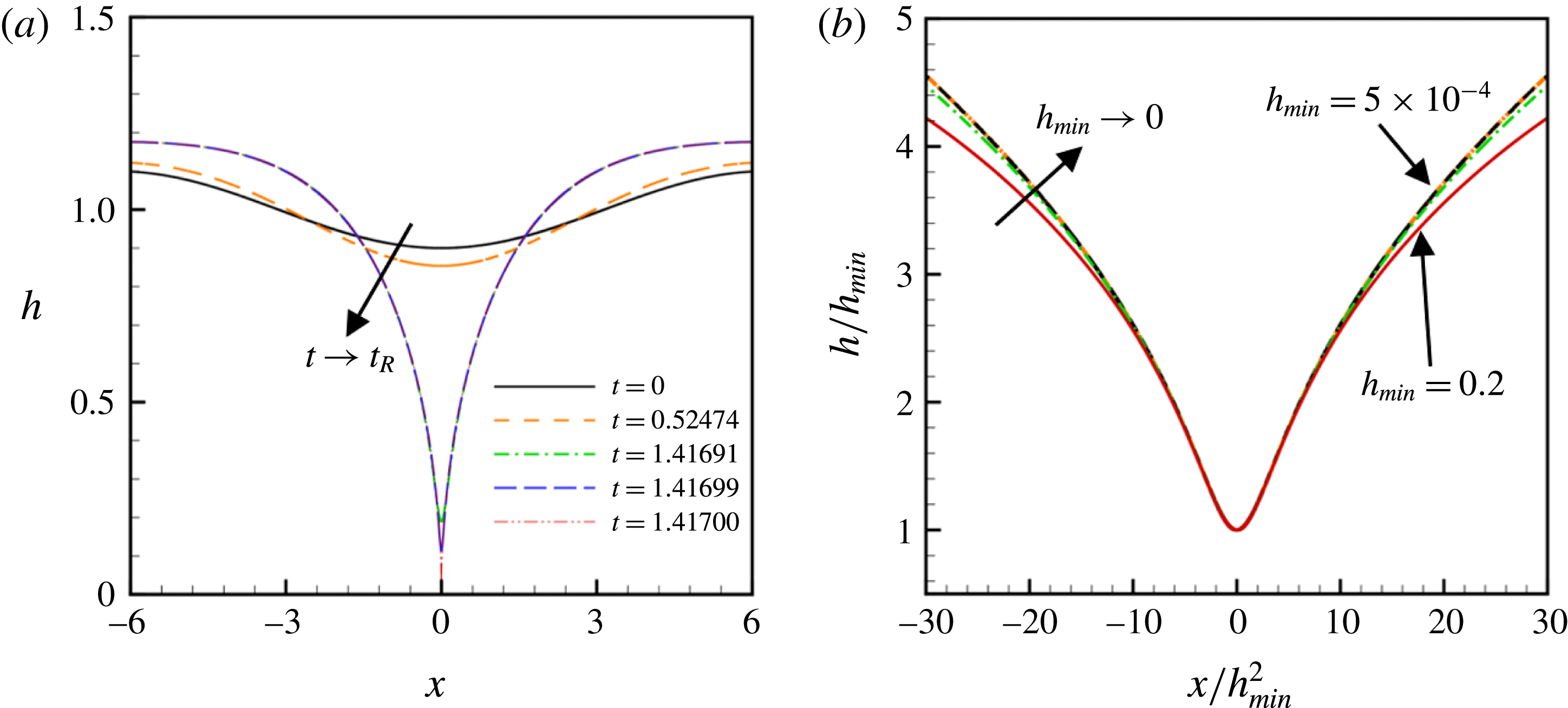
(a) Computed instantaneous film profiles
 $h=h(x,t)$
as a function of the lateral coordinate
 $x$
for a thinning film of power-law index of
 $n=0.83$
. Starting with a slightly deformed profile at
 $t=0$
, the interface profiles are seen to steepen as
 $t\rightarrow t_{R}$
and rupture nears. Here, the rupture time
 $t_{R}\doteq 1.41700$
. (b) Rescaled interface shape
 $h/h_{min}$
as a function of rescaled lateral coordinate
 $x/h_{min}^{2}$
at several instants in time for the thinning power-law film of part (a). The rescaled transient profiles are shown for values of
 $5\times 10^{-4}\leqslant h_{min}\leqslant 2.0\times 10^{-1}$
. Each rescaled interface shape corresponding to a successively smaller value of
 $h_{min}$
is such that the value of the minimum film thickness is approximately half that of the previously shown rescaled profile. The rescaled profiles are seen to approach or collapse onto a similarity profile as
 $h_{min}\rightarrow 0$
.

Figure 3 shows the computed variation with time remaining until rupture of several quantities of interest in the rupture zone for the film of power-law index of
 $n=0.83$
. As shown below, in this situation and in all the other ones that have been considered, the minimum film thickness is always located at
 $x=0$
, viz.
 $h_{min}=h(0,t)$
, and therefore the film always ruptures symmetrically at
 $x=0$
so that
 $x_{R}=0$
and
 $x^{\prime }=x$
. The simulation results of figure 3(a) show that
 $h_{min}$
decreases with
 $\unicode[STIX]{x1D70F}$
as
 $h_{min}\sim \unicode[STIX]{x1D70F}^{0.172}$
, a result that is in excellent agreement with the theoretical prediction (cf. (4.7) and (4.8)) that
 $h_{min}\sim \unicode[STIX]{x1D70F}^{n/(n+4)}|_{n=0.83}\equiv \unicode[STIX]{x1D70F}^{0.172}$
.
The scaling of the lateral length has been determined in two different ways. The first method involves determining how the computed value of the film’s curvature,
 $\unicode[STIX]{x2202}^{2}h/\unicode[STIX]{x2202}x^{2}$
, evaluated at
 $x=0$
varies with
 $\unicode[STIX]{x1D70F}$
and using this result, along with the known scaling for
 $h$
, to determine the scaling for
 $x$
. The curvature is expected to scale as
 $$\begin{eqnarray}\frac{\unicode[STIX]{x2202}^{2}h}{\unicode[STIX]{x2202}x^{2}}\sim \frac{h}{x^{2}}\sim \unicode[STIX]{x1D70F}^{\unicode[STIX]{x1D6FC}-2\unicode[STIX]{x1D6FD}}\sim \unicode[STIX]{x1D70F}^{-3n/(n+4)}.\end{eqnarray}$$
Figure 3(b) shows the computed value of the curvature at
 $x=0$
blows up with
 $\unicode[STIX]{x1D70F}$
as
 $(\unicode[STIX]{x2202}^{2}h/\unicode[STIX]{x2202}x^{2})(0,t)\sim \unicode[STIX]{x1D70F}^{-0.515}$
, a result that is in excellent accord with the theoretical prediction of
 $(\unicode[STIX]{x2202}^{2}h/\unicode[STIX]{x2202}x^{2})(0,t)\sim \unicode[STIX]{x1D70F}^{-3n/(n+4)}|_{n=0.83}\sim \unicode[STIX]{x1D70F}^{-0.515}$
. Since the value of the curvature predicted from simulations scales as
 $\unicode[STIX]{x1D70F}^{-0.515}$
, it is straightforward to combine this result with the simulation result that
 $h\sim \unicode[STIX]{x1D70F}^{0.172}$
to determine that the lateral length scales as
 $x\sim \unicode[STIX]{x1D70F}^{0.344}$
. This result is also in excellent agreement with theory as it follows from (4.7) and (4.8) that when
 $n=0.83$
, the value of the lateral scaling exponent should be
 $2(0.172)=0.344$
. The second independent method for determining the scaling of the lateral length is based on monitoring the variation with
 $\unicode[STIX]{x1D70F}$
of the lateral location at which the film thickness equals some multiple of the minimum film thickness, which is herein taken to be
 $1.001h_{min}$
. This latter method directly yields the value of the lateral scaling exponent. Reassuringly, the value of the lateral scaling exponent determined in this manner has been found to be identical to that determined by the first approach. Furthermore, changing the lateral location at which this determination is made, e.g. from
 $1.001h_{min}$
to
 $1.002h_{min}$
, has no effect whatsoever on the value of the scaling exponent
 $\unicode[STIX]{x1D6FD}$
determined from simulations.
It is expected from theory that the lateral velocity
 $u$
should scale as
 $$\begin{eqnarray}u\sim \frac{x}{\unicode[STIX]{x1D70F}}\sim \unicode[STIX]{x1D70F}^{\unicode[STIX]{x1D6FD}-1}\sim \unicode[STIX]{x1D70F}^{(n-4)/(n+4)}.\end{eqnarray}$$
Thus, when
 $n=0.83$
, the scaling exponent of the lateral velocity should equal
 $-0.656$
. Figure 3(c) shows that the lateral velocity
 $u^{\prime }$
computed at the lateral location
 $x^{\prime }$
where
 $h(x^{\prime },t)=1.001h_{min}$
diverges with
 $\unicode[STIX]{x1D70F}$
as
 $u^{\prime }\sim \unicode[STIX]{x1D70F}^{-0.656}$
, in accord with theory.
Figure 3(d) shows that the computed variation of the viscosity
 $\unicode[STIX]{x1D707}^{\prime }$
, calculated at lateral location
 $x^{\prime }$
, with
 $\unicode[STIX]{x1D70F}$
is seen to follow the scaling behaviour that
 $\unicode[STIX]{x1D707}^{\prime }\sim \unicode[STIX]{x1D70F}^{0.141}$
. This simulation result is also seen to accord nicely with theory in that it follows from (4.13) that
 $\unicode[STIX]{x1D707}\sim \unicode[STIX]{x1D70F}^{4(1-n)/(n+4)}|_{n=0.83}\sim \unicode[STIX]{x1D70F}^{0.141}$
.
Figure 4(a) shows at several instants in time computed profiles of a thinning film of power-law index of
 $n=0.83$
. As has already been stated, the minimum film thickness can be seen to be located throughout the thinning at
 $x=0$
and, therefore, the film ruptures symmetrically at
 $x=0$
. According to theory (cf. (4.7) and (4.8)),
 $h=\unicode[STIX]{x1D70F}^{\unicode[STIX]{x1D6FC}}H(\unicode[STIX]{x1D702})$
and
 $\unicode[STIX]{x1D702}=x/\unicode[STIX]{x1D70F}^{\unicode[STIX]{x1D6FD}}=x/\unicode[STIX]{x1D70F}^{2\unicode[STIX]{x1D6FC}}$
. Therefore, it also follows from theory that
 $h_{min}=\unicode[STIX]{x1D70F}^{\unicode[STIX]{x1D6FC}}H(0)$
and hence
 $$\begin{eqnarray}\frac{h}{h_{min}}=\frac{H(\unicode[STIX]{x1D702})}{H(0)}\quad \text{and}\quad \unicode[STIX]{x1D702}=\frac{x}{[h_{min}/H(0)]^{2}}.\end{eqnarray}$$
Therefore, to demonstrate the self-similarity of the computed film profiles, rescaled interface shapes
 $h/h_{min}$
at certain instances in time determined from computations are plotted in figure 4(b) as a function of the rescaled coordinate
 $x/h_{min}^{2}$
, which is proportional to the similarity variable
 $\unicode[STIX]{x1D702}$
. The rescaled shapes are seen to collapse nicely onto a single profile in the figure as
 $h_{min}\rightarrow 0$
, demonstrating the self-similarity of the dynamics as the rupture singularity is approached. It is noteworthy that plotting the computed solutions in the manner indicated sidesteps the necessity of determining
 $\unicode[STIX]{x1D70F}$
from simulations and therefore is preferable to plotting
 $h/h_{min}$
as a function of
 $\unicode[STIX]{x1D702}$
.
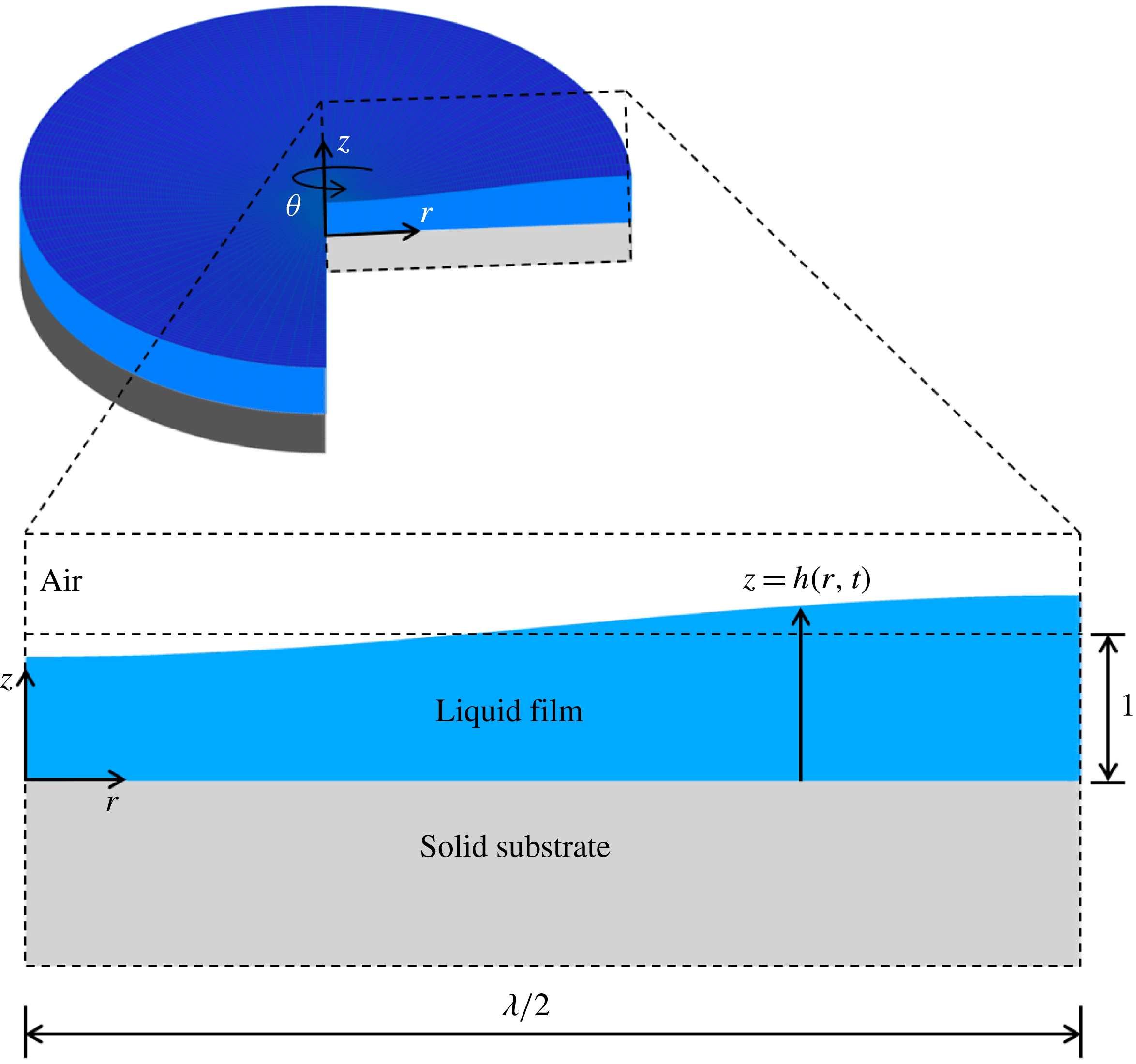
Point rupture. Top: perspective view of a film on a substrate showing the deformed interface over a lateral or radial extent corresponding to one half of a wavelength
 $\unicode[STIX]{x1D706}/2$
of the imposed perturbation. Bottom: a blow-up or zoomed-in cross-sectional view of the film over a lateral extent corresponding to one half of a wavelength of the imposed perturbation. Here, the problem domain is
 $0\leqslant r\leqslant \unicode[STIX]{x1D706}/2$
.

5 Axisymmetric or point rupture in the lubrication limit
In this section, the initially flat surface of the film is subjected to a sinusoidal shape perturbation that is axisymmetric or invariant in the
 $\unicode[STIX]{x1D703}$
-direction and has wavelength
 $\unicode[STIX]{x1D706}$
in the lateral (radial) or
 $r$
-direction, where
 $r\equiv \tilde{r}/l_{c}$
, as shown in figure 5. Since the perturbation is three-dimensional but axisymmetric in nature, equation (3.1) subjected to boundary conditions (3.5) and (3.6) is solved in cylindrical polar coordinates such that
 $\boldsymbol{v}_{H}=u(r,z,t)\boldsymbol{e}_{r}$
and
 $\unicode[STIX]{x1D735}_{H}=\boldsymbol{e}_{r}(\unicode[STIX]{x2202}/\unicode[STIX]{x2202}r)+\boldsymbol{e}_{\unicode[STIX]{x1D703}}(1/r)(\unicode[STIX]{x2202}/\unicode[STIX]{x2202}\unicode[STIX]{x1D703})$
, where
 $\boldsymbol{e}_{r}$
and
 $\boldsymbol{e}_{\unicode[STIX]{x1D703}}$
are unit vectors in the
 $r$
- and
 $\unicode[STIX]{x1D703}$
-directions, to arrive at the following expression for the dimensionless lateral velocity
 $u(r,z,t)$
 $$\begin{eqnarray}u(r,z,t)=\frac{n}{n+1}\frac{|\unicode[STIX]{x2202}p/\unicode[STIX]{x2202}r|}{\unicode[STIX]{x2202}p/\unicode[STIX]{x2202}r}m^{1/n-1}\left|\frac{\unicode[STIX]{x2202}p}{\unicode[STIX]{x2202}r}\right|^{1/n}[(h-z)^{1/n+1}-h^{1/n+1}],\end{eqnarray}$$
where
 $h(r,t)$
is the local film thickness. In arriving at (5.1), use is made of the fact that in cylindrical polar coordinates, the dimensionless viscosity (cf. (3.4)) and the dimensionless fluid pressure
 $p(r,t)$
are given by
 $$\begin{eqnarray}\unicode[STIX]{x1D707}=\left|m\frac{\unicode[STIX]{x2202}u}{\unicode[STIX]{x2202}z}\right|^{n-1}\end{eqnarray}$$
and
 $$\begin{eqnarray}p=\frac{1}{h^{3}}-\frac{3}{r}\frac{\unicode[STIX]{x2202}}{\unicode[STIX]{x2202}r}\left(r\frac{\unicode[STIX]{x2202}h}{\unicode[STIX]{x2202}r}\right).\end{eqnarray}$$
When the expression for
 $u$
given by (5.1) is plugged into (3.3), a spatially one-dimensional, nonlinear evolution equation results that governs the variation of the film thickness with the dimensionless lateral coordinate
 $r$
and dimensionless time
 $t$
 $$\begin{eqnarray}\frac{\unicode[STIX]{x2202}h}{\unicode[STIX]{x2202}t}-\frac{|\unicode[STIX]{x2202}p/\unicode[STIX]{x2202}r|}{\unicode[STIX]{x2202}p/\unicode[STIX]{x2202}r}m^{1/n-1}\frac{\unicode[STIX]{x2202}}{\unicode[STIX]{x2202}r}\left[\frac{n}{2n+1}\left|\frac{\unicode[STIX]{x2202}p}{\unicode[STIX]{x2202}r}\right|^{1/n}h^{1/n+2}\right]=0.\end{eqnarray}$$
Because of the periodic nature of the imposed perturbation, it is sufficient to solve the problem over the spatial domain spanning one half of the wavelength of the imposed perturbation, viz.
 $0\leqslant r\leqslant \unicode[STIX]{x1D706}/2$
, as shown in figure 5. The 1-D evolution equation is solved subject to the boundary conditions that
 $$\begin{eqnarray}\displaystyle & \displaystyle \frac{\unicode[STIX]{x2202}h}{\unicode[STIX]{x2202}r}=0\quad \text{at }r=0\text{ and }r=\unicode[STIX]{x1D706}/2, & \displaystyle\end{eqnarray}$$
 $$\begin{eqnarray}\displaystyle & \displaystyle Q=0\quad \text{at }r=0\text{ and }r=\unicode[STIX]{x1D706}/2, & \displaystyle\end{eqnarray}$$
where
 $Q$
is the flow rate. Boundary conditions given by (5.6) are conveniently imposed in the Galerkin finite-element formulation which through the usual integration by parts gives rise to end point terms at both
 $r=0$
and
 $r=\unicode[STIX]{x1D706}/2$
that are proportional to
 $Q$
. Physically, imposing
 $Q=0$
at
 $r=0$
ensures that
 $r=0$
is not a source or a sink of fluid. Imposing
 $Q=0$
at
 $r=\unicode[STIX]{x1D706}/2$
ensures that no fluid enters or leaves the computational domain at
 $r=\unicode[STIX]{x1D706}/2$
. The initial condition is given by
 $$\begin{eqnarray}h(r,0)=1-\unicode[STIX]{x1D6FF}\cos (2\unicode[STIX]{x03C0}r/\unicode[STIX]{x1D706}),\end{eqnarray}$$
where
 $\unicode[STIX]{x1D6FF}$
again stands for the amplitude of the perturbation that is imposed to initiate the thinning of the film.
5.1 Scaling and self-similarity
Once again, the film profile is expected to be self-similar in the vicinity of the location where the film thickness is minimum as the space–time rupture singularity
 $(r=0,t=t_{R})$
is approached. Hence, the film profile in the vicinity of the rupture point
 $r=0$
should have the functional form
 $$\begin{eqnarray}h(r,\unicode[STIX]{x1D70F})=\unicode[STIX]{x1D70F}^{\unicode[STIX]{x1D6FC}}H(\unicode[STIX]{x1D702}),\quad \unicode[STIX]{x1D702}=r/\unicode[STIX]{x1D70F}^{\unicode[STIX]{x1D6FD}},\end{eqnarray}$$
where
 $\unicode[STIX]{x1D70F}\equiv t_{R}-t$
is the dimensionless time remaining until rupture,
 $r$
, aside from being the radial coordinate, is the lateral extent of this rupture zone,
 $\unicode[STIX]{x1D702}$
is the similarity variable,
 $\unicode[STIX]{x1D6FC}$
and
 $\unicode[STIX]{x1D6FD}$
are the scaling exponents for
 $h$
and
 $r$
, respectively, and
 $H(\unicode[STIX]{x1D702})$
is the scaling function for the film profile in similarity space. Following the same approach as the one that was used to determine the scaling exponents in the case of line rupture, the scaling exponents
 $\unicode[STIX]{x1D6FC}$
and
 $\unicode[STIX]{x1D6FD}$
in (5.8) can be readily shown to be given by
 $$\begin{eqnarray}\unicode[STIX]{x1D6FC}=\frac{n}{n+4},\quad \unicode[STIX]{x1D6FD}=\frac{2n}{n+4}.\end{eqnarray}$$
From the dimensionless form of (3.1) and (5.2) and (5.3) and with the scaling exponents given by (5.9), the van der Waals, surface tension or capillary and viscous stresses can be shown to scale as
 $\unicode[STIX]{x1D70F}^{-5n/(n+4)}$
. For future reference, it is worth noting that fluid viscosity in the thinning film scales as
 $\unicode[STIX]{x1D70F}^{4(1-n)/(n+4)}$
.
It is readily seen that in the Newtonian limit
 $(n=1)$
, the expressions in (5.9) for the scaling exponents take on the values of
 $\unicode[STIX]{x1D6FC}=1/5$
and
 $\unicode[STIX]{x1D6FD}=2/5$
and all three stresses diverge as
 $\unicode[STIX]{x1D70F}^{-1}$
in agreement with previous work on rupture of Newtonian films (Zhang & Lister Reference Zhang and Lister1999).
5.2 Simulation of point rupture in the lubrication limit
The spatially fourth-order nonlinear evolution equation (5.4) subject to boundary conditions (5.5) and (5.6) and initial condition (5.7) with
 $\unicode[STIX]{x1D6FF}=0.1$
is solved numerically using the same Galerkin finite-element-based algorithm that has been employed earlier to simulate line rupture to verify the scaling exponents that have just been determined and to demonstrate the self-similarity of the film profiles in the rupture zone. In the simulations, the wavelength of the imposed perturbation is taken to equal
 $\unicode[STIX]{x1D706}=4\unicode[STIX]{x03C0}$
. In all of the simulations that have been carried out, it is found that the minimum film thickness is always located at
 $r=0$
, viz.
 $h_{min}=h(0,t)$
, and that the film always ruptures at
 $r=0$
.
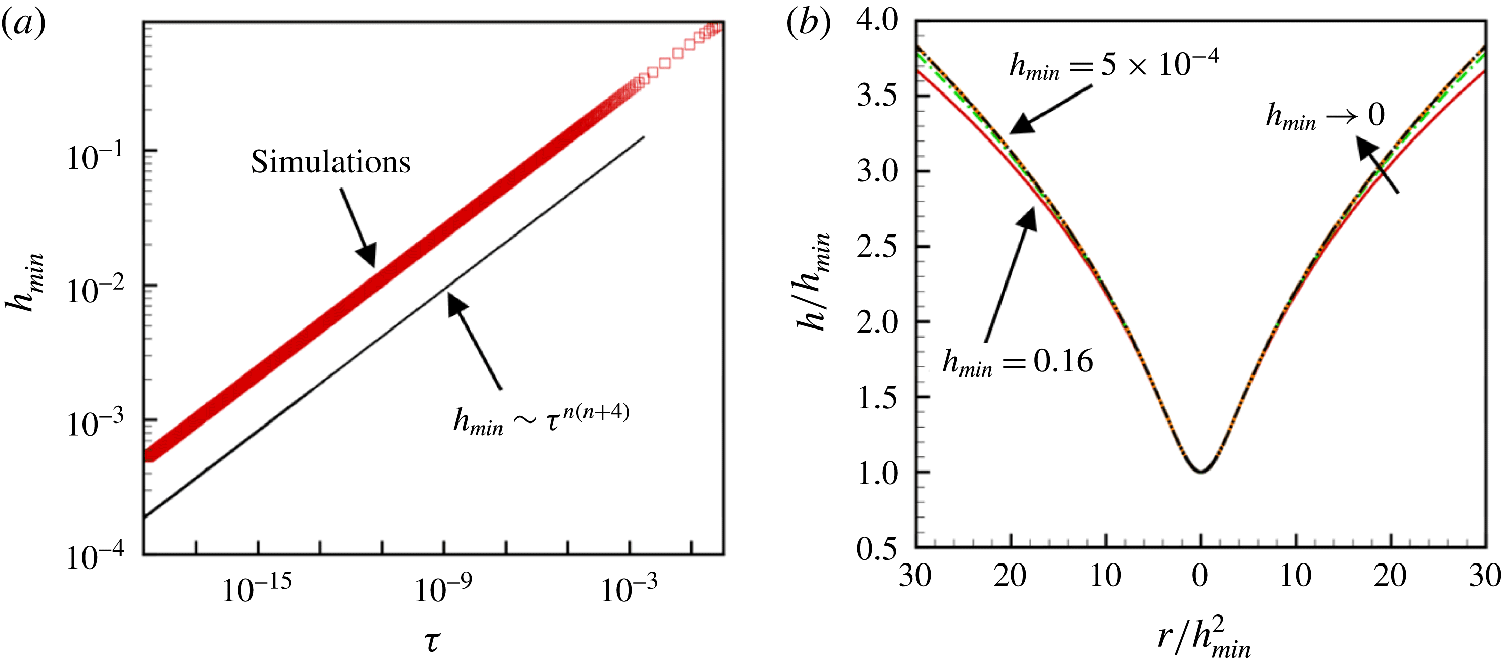
(a) Variation of the minimum film thickness
 $h_{min}$
with time remaining until rupture during thinning of a film of power-law index of
 $n=0.85$
undergoing point rupture: simulations (data points) and scaling theory predictions (straight line with indicated dependency on time remaining until rupture
 $\unicode[STIX]{x1D70F}$
). (b) Rescaled interface shape
 $h/h_{min}$
as a function of rescaled lateral coordinate
 $r/h_{min}^{2}$
at several instants in time determined from simulations during thinning of the film of part (a). The rescaled transient profiles are shown for values of
 $5\times 10^{-4}\leqslant h_{min}\leqslant 1.6\times 10^{-1}$
. Each rescaled interface shape corresponding to a successively smaller value of
 $h_{min}$
is such that the value of the minimum film thickness is approximately half that of the previously shown rescaled profile. The rescaled profiles are seen to approach or collapse onto a similarity profile as
 $h_{min}\rightarrow 0$
.

Figure 6(a) shows the computed variation with time remaining until rupture of the minimum film thickness for a thinning film of power-law index of
 $n=0.85$
. Monitoring the computed variation of
 $h_{min}$
with
 $\unicode[STIX]{x1D70F}$
as well as those of the curvature, lateral (radial) velocity and viscosity (not shown) reveal that the variations predicted from simulations are all in excellent accord with theory.
Figure 6(b) shows rescaled interface shapes
 $h/h_{min}$
at certain instances in time determined from computations as a function of the rescaled coordinate
 $r/h_{min}^{2}$
during the thinning of the film of power-law index of
 $n=0.85$
. The rescaled shapes are seen to collapse nicely onto a single profile as
 $h_{min}\rightarrow 0$
, demonstrating the self-similarity of the dynamics as the film approaches rupture.
6 Breakdown of lubrication approximation and role of inertia
As discussed in standard books on fluid mechanics (Deen Reference Deen1998; Leal Reference Leal2007) and shown in appendix A, two key assumptions that have been made in analysing film rupture concern the applicability of the lubrication approximation. The first of these pertains to the validity of the long-wavelength approximation. As the initial aspect ratio of the film
 $\unicode[STIX]{x1D700}(0)\equiv \unicode[STIX]{x1D716}\equiv h_{0}/l_{c}\ll 1$
(in this section, we use the notation
 $\unicode[STIX]{x1D700}(\tilde{t})$
to denote the instantaneous aspect ratio of the film to distinguish it from the aspect ratio at the initial instant,
 $\unicode[STIX]{x1D716}$
), the use of the lubrication approximation is justified during the initial stages of the thinning. If
 $\tilde{h}(\tilde{t})$
and
 $\tilde{l}(\tilde{t})$
denote the film thickness and the lateral length scale at time
 $\tilde{t}$
, the film aspect ratio at time
 $\tilde{t}$
is given by
 $\unicode[STIX]{x1D700}(\tilde{t})\equiv \tilde{h}_{min}(\tilde{t})/\tilde{l}(\tilde{t})$
. From the results of this paper,
 $\tilde{h}_{min}(\tilde{t})\sim h_{0}\unicode[STIX]{x1D70F}^{n/(n+4)}$
. The lateral length, however, scales as
 $$\begin{eqnarray}\displaystyle \tilde{l}(\tilde{t})\sim l_{c}\unicode[STIX]{x1D70F}^{2n/(n+5)} & {\sim} & \displaystyle l_{c}\left[\frac{\tilde{h}_{min}(\tilde{t})}{h_{0}}\right]^{2}\end{eqnarray}$$
 $$\begin{eqnarray}\displaystyle & {\sim} & \displaystyle \frac{[\tilde{h}_{min}(\tilde{t})]^{2}}{d}.\end{eqnarray}$$
Therefore, the aspect ratio at time
 $\tilde{t}$
is given by
 $$\begin{eqnarray}\unicode[STIX]{x1D700}(\tilde{t})=\frac{\tilde{h}_{min}(\tilde{t})}{\tilde{l}(\tilde{t})}\sim \frac{d}{\tilde{h}_{min}(\tilde{t})}.\end{eqnarray}$$
Since the continuum approximation fails when the minimum film thickness becomes of the order of the molecular length scale, it is seen from the last equation that the long-wavelength approximation is valid throughout the thinning and fails at the same time as the continuum approximation does.
In order for the lubrication approximation to be valid, the film must not only be slender (as discussed in the previous paragraph) but the modified Reynolds number
 $Re^{\ast }$
which multiplies the inertial terms in the dimensionless Cauchy momentum equation (cf. Deen (Reference Deen1998) and appendix A) and is given by the product of the film aspect ratio and the Reynolds number
 $Re$
, the ratio of inertial to viscous forces, must be small. Zhang & Lister (Reference Zhang and Lister1999) have shown that inertia remains negligible until rupture during thinning of films of Newtonian fluids. For power-law fluids, as the film’s viscosity decreases due to the deformation-rate-thinning rheology of such fluids,
 $Re$
can grow and the possibility exists that the
 $Re^{\ast }$
can become of order one or larger. The instantaneous value of
 $Re^{\ast }$
can be calculated as
 $$\begin{eqnarray}\displaystyle Re^{\ast }(\tilde{t}) & = & \displaystyle Re(\tilde{t})\unicode[STIX]{x1D700}(\tilde{t})=\frac{\unicode[STIX]{x1D70C}\tilde{u} (\tilde{t})\tilde{h}(\tilde{t})}{\tilde{\unicode[STIX]{x1D707}}(\tilde{t})}\frac{\tilde{h}(\tilde{t})}{\tilde{l}(\tilde{t})}\end{eqnarray}$$
 $$\begin{eqnarray}\displaystyle & = & \displaystyle \frac{\unicode[STIX]{x1D70C}h_{0}^{2}}{\unicode[STIX]{x1D707}_{0}t_{c}}\unicode[STIX]{x1D70F}^{(5n-8)/(n+4)}=\frac{1}{3}\frac{h_{0}}{l_{\unicode[STIX]{x1D707}}}\frac{1}{(h_{0}/d)^{4}}\unicode[STIX]{x1D70F}^{(5n-8)/(n+4)},\end{eqnarray}$$
where
 $l_{\unicode[STIX]{x1D707}}=\unicode[STIX]{x1D707}_{0}^{2}/\unicode[STIX]{x1D70C}\unicode[STIX]{x1D70E}$
is the viscous length (see, e.g. Eggers Reference Eggers1997). Since
 $\tilde{h}_{min}(\tilde{t})\sim h_{0}\unicode[STIX]{x1D70F}^{n/(n+4)}$
, equation (6.5) can be used to determine the value of the minimum film thickness at which the modified Reynolds number becomes of order one,
 $Re^{\ast }\sim 1$
:
 $$\begin{eqnarray}\frac{\tilde{h}_{min}}{d}\sim \left[\left(\frac{h_{0}}{l_{\unicode[STIX]{x1D707}}}\right)^{8(1-n)}\left(\frac{d}{l_{\unicode[STIX]{x1D707}}}\right)^{9n-8}\right]^{1/(8-5n)}\equiv \left[Oh^{16(n-1)}\left(\frac{d}{l_{\unicode[STIX]{x1D707}}}\right)^{9n-8}\right]^{1/(8-5n)},\end{eqnarray}$$
where the ratio
 $l_{\unicode[STIX]{x1D707}}/h_{0}$
is the square of the dimensionless group referred to as the Ohnesorge number
 $Oh$
, viz.
 $Oh=\sqrt{l_{\unicode[STIX]{x1D707}}/h_{0}}=\unicode[STIX]{x1D707}_{0}/\sqrt{\unicode[STIX]{x1D70C}\unicode[STIX]{x1D70E}h_{0}}$
. For a Newtonian fluid
 $(n=1)$
, equation (6.6) reduces to
 $$\begin{eqnarray}\frac{\tilde{h}_{min}}{d}\sim \left(\frac{d}{l_{\unicode[STIX]{x1D707}}}\right)^{1/3}.\end{eqnarray}$$
Since typically
 $d<l_{\unicode[STIX]{x1D707}}$
(for example, whereas the molecular length scale is of the order of nanometres, the viscous length is approximately 14 nm for water,
 $200~\unicode[STIX]{x03BC}\text{m}$
for a 85 % glycerol–water solution and 2 cm for pure glycerol (Timmermans Reference Timmermans1960)),
 $\tilde{h}_{min}$
has to fall below the molecular length scale for inertia to come into play for a Newtonian fluid. For power-law fluids, an interesting limit is that as
 $n\rightarrow 0$
in (6.6):
 $$\begin{eqnarray}\frac{\tilde{h}_{min}}{d}\sim \frac{h_{0}}{d}.\end{eqnarray}$$
Equation (6.8) shows that inertia would be important during the entire period of thinning for films of highly deformation-rate-thinning power-law fluids or ones having vanishingly small values of the power-law index
 $n$
.
When neither
 $n=1$
nor
 $n\rightarrow 0$
but
 $n\geqslant 8/9$
, and if
 $h_{0}<l_{\unicode[STIX]{x1D707}}$
and
 $d<l_{\unicode[STIX]{x1D707}}$
,
 $\tilde{h}_{min}$
will have to fall below
 $d$
in order for inertia to become important during film thinning. Therefore, it is unlikely for inertia to become important during thinning of power-law films of power-law index of
 $n\geqslant 8/9$
. If, however,
 $n\leqslant 8/9$
and
 $h_{0}<l_{\unicode[STIX]{x1D707}}$
and
 $d<l_{\unicode[STIX]{x1D707}}$
, it is possible that the modified Reynolds number can become of order one when
 $\tilde{h}_{min}$
is greater than
 $d$
. In particular, if the film fluid is acrylic paint (Huisman et al.
Reference Huisman, Friedman and Taborek2012), a power-law fluid with properties of
 $A=10^{-19}~\text{J}$
,
 $\unicode[STIX]{x1D70E}=0.05~\text{N}~\text{m}^{-1}$
,
 $\unicode[STIX]{x1D707}_{0}m^{n-1}=35.6~\text{Pa}~\text{s}^{n}$
,
 $\unicode[STIX]{x1D70C}=1150~\text{kg}~\text{m}^{-3}$
and
 $n=0.44$
, and the initial film thickness
 $h_{0}=10^{-6}~\text{m}$
(
 $1~\unicode[STIX]{x03BC}\text{m}$
or 1000 nm), inertia can become important once the normalized minimum film thickness reaches a value of
 $\tilde{h}_{min}/d\sim 50.8$
or the minimum film thickness
 $\tilde{h}_{min}$
falls below 28.6 nm. Hence, for power-law fluids of sufficiently small power-law index
 $n$
, the possibility exists that inertia will become important before the continuum approximation breaks down.
Therefore, equation (6.6) can be used to determine, for different films of power-law fluids, the value of the scaled minimum film thickness
 $\tilde{h}_{min}/d$
below which inertia will come into play during film thinning as a function of either (i) the ratio
 $l_{\unicode[STIX]{x1D707}}/h_{0}$
, the ratio
 $d/h_{0}$
and power-law index
 $n$
or equivalently (ii) the Ohnesorge number
 $Oh=\sqrt{l_{\unicode[STIX]{x1D707}}/h_{0}}=\unicode[STIX]{x1D707}_{0}/\sqrt{\unicode[STIX]{x1D70C}\unicode[STIX]{x1D70E}h_{0}}$
(a dimensionless group that equals the ratio of viscous force to the square root of the product of surface tension and inertial forces), the van der Waals number
 $A^{\ast }\equiv A/(6\unicode[STIX]{x03C0}\unicode[STIX]{x1D70E}{h_{0}}^{2})=(1/3)(d/h_{0})^{2}$
(a dimensionless group that represents the relative importance of intermolecular force to surface tension force) and power-law index
 $n$
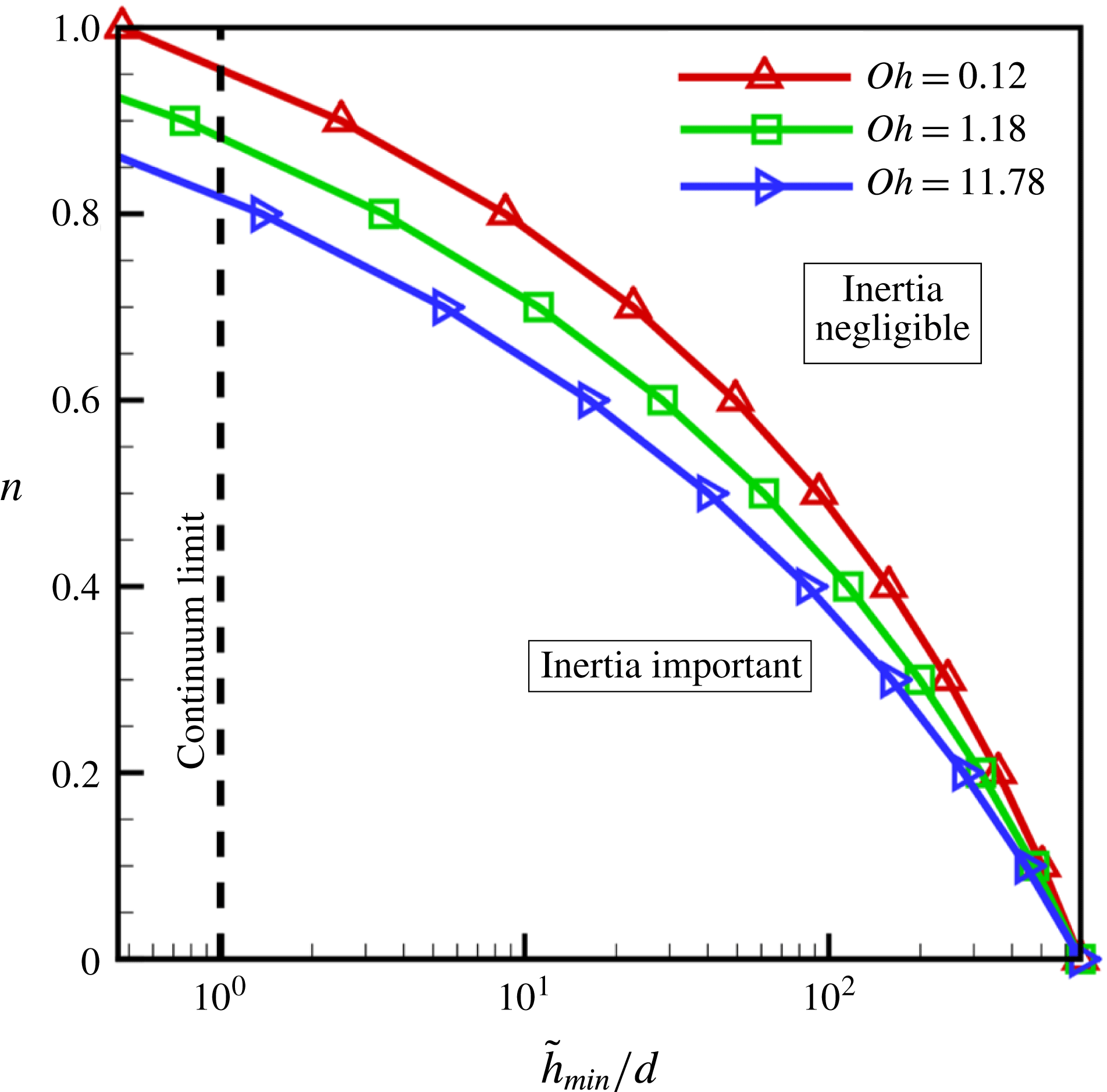
. The results of such an analysis can be used to construct a phase diagram as in figure 7 that shows for a fixed value of
 $A^{\ast }=7.37\times 10^{-7}$
(for the film of acrylic paint referred to above,
 $A^{\ast }=O(10^{-7})$
) and Ohnesorge numbers spanning two orders of magnitude between approximately 0.1 and 10, the variation of the critical value of the normalized film thickness
 $\tilde{h}_{min}/d$
at which inertia becomes important with the power-law index
 $n$
. In accord with intuition, this figure makes it clear that for fixed
 $n$
, the lower the value of
 $Oh$
or the less viscous the film fluid, the larger is the value of the normalized film thickness at which inertia becomes important. Thus, the study of the dynamics of thinning of films of power-law fluids on a substrate is incomplete without considering the role of inertia, which is taken up in the following two sections.
Phase diagram that shows for films of different power-law fluids each of which is characterized by a given value of
 $Oh$
,
 $A^{\ast }$
and
 $n$
whether inertia can become important during film thinning. Here, results are shown for three different values of the Ohnesorge number,
 $Oh=0.12,1.18$
and
 $11.78$
, at a fixed value of the ratio of van der Waals to surface tension force of
 $A^{\ast }=7.37\times 10^{-7}$
, and over the entire range of possible values of the power-law index
 $n$
. For a film of given
 $n$
, the dynamics starts in a regime where inertia is negligible (in the region to the right of the curves in the figure) and, as the film continues to thin and
 $\tilde{h}_{min}/d$
continues to decrease, the dynamics can undergo a transition from the inertialess regime to one where inertia is important if the value of
 $\tilde{h}_{min}/d$
can attain a value that lies to the left of the appropriate curve in the figure and provided that the transition can occur before the continuum limit is reached (which is indicated by the vertical dashed line). It is clear that for sufficiently small values of the power-law index
 $n$
, inertia becomes significant long before the continuum limit is reached. (Note: for a fixed value of
 $Oh$
, a curve in the phase diagram is determined from (6.6) using the relationship that
 $d/l_{\unicode[STIX]{x1D707}}=\sqrt{3A^{\ast }}/Oh^{2}$
.)

7 Problem statement for analysis of film rupture with inertia and summary of approach used in two-dimensional simulations
In the remainder of the paper, the effect of inertia on thinning and rupture of a thin film of undisturbed thickness
 $h_{0}$
is determined by solving the spatially two-dimensional (2-D), transient Cauchy momentum and continuity equations ((2.2) and (2.1) in § 2). Given the equality of the scaling exponents governing the dynamics of thinning in the vicinity of the singularity in the planar (or two-dimensional rupture) and axisymmetric (or point rupture) geometries, this more involved analysis requiring the solution of the free boundary problem comprised of a transient, nonlinear system of spatially two-dimensional partial differential equations is performed only for the case of line rupture. Therefore, in this situation, the dynamics is translationally symmetric or invariant in the
 ${\tilde{y}}$
-direction and the problem domain is the portion of the
 $(\tilde{x},\tilde{z})$
-plane that lies within the liquid film over a horizontal distance equal to one half the wavelength
 $\tilde{\unicode[STIX]{x1D706}}/2$
of the initial perturbation that is imposed on the film’s surface, i.e. the domain is the region that is bounded below by the solid substrate located at
 $(0\leqslant \tilde{x}\leqslant \tilde{\unicode[STIX]{x1D706}}/2,\tilde{z}=0)$
, bounded above by the free surface
 $S(\tilde{t})$
and bounded on the sides by the symmetry planes located at
 $\tilde{x}=0$
and
 $\tilde{\unicode[STIX]{x1D706}}/2$
. Along the solid substrate, the adherence boundary condition given by (2.3) is imposed. At the film’s surface, kinematic and traction boundary conditions given by (2.4) and (2.5) are imposed. Along the two symmetry planes, the horizontal (lateral) velocity and the tangential stress are set equal to zero. At
 $\tilde{x}=0$
and
 $\tilde{x}=\tilde{\unicode[STIX]{x1D706}}/2$
, symmetry requires that the free surface has zero slope at both locations.
In contrast to the previous sections where different characteristic lengths are employed in the horizontal and vertical directions, here a single characteristic length
 $h_{c}\equiv h_{0}$
is used to non-dimensionalize both the horizontal and vertical coordinates, viz.
 $x\equiv \tilde{x}/h_{c}$
and
 $z\equiv \tilde{z}/h_{c}$
. As in the previous sections, here variables without tildes over them denote the dimensionless counterparts of those with tildes. Because the critical wavelength for instability
 $\tilde{\unicode[STIX]{x1D706}}_{c}=2\unicode[STIX]{x03C0}h_{0}^{2}/d$
, the lateral extent of the film in the horizontal direction or the maximum value of the dimensionless
 $x$
-coordinate can range between 10
 $^{3}$
and 10
 $^{5}$
, thereby making the problem fall in the category of challenging multiscale flow problems involving highly disparate length scales. In anticipation of computing solutions for which inertia is important, the inertio–capillary time is chosen as the characteristic time scale, viz.
 $t_{c}\equiv \sqrt{\unicode[STIX]{x1D70C}h_{0}^{3}/\unicode[STIX]{x1D70E}}$
, and the characteristic velocity is chosen as the ratio of the characteristic length and time scales, viz.
 $u_{c}\equiv h_{c}/t_{c}$
. As characteristic pressure, viscosity and strain-rate scales, the same ones as those used in § 4 are adopted here. With the scales just introduced, the dynamics is then governed by two dimensionless groups: the Ohnesorge number
 $Oh\equiv \unicode[STIX]{x1D707}_{0}/\sqrt{\unicode[STIX]{x1D70C}h_{0}\unicode[STIX]{x1D70E}}$
and the dimensionless van der Waals number
 $A^{\ast }\equiv A/6\unicode[STIX]{x03C0}\unicode[STIX]{x1D70E}h_{0}^{2}$
, both of which have already been introduced in the previous section.
As the rate at which viscosity falls with increasing deformation rate increases as
 $n$
decreases, we expect the relative importance of inertia compared to viscous force to grow as a film thins for fluids of small
 $n$
. A dominant balance argument in such cases reveals that inertial, capillary and van der Waals forces are in balance as the film approaches rupture and gives to rise to an inertial scaling regime where the scaling exponents are independent of the power-law index
 $n$
:
 $$\begin{eqnarray}h\sim \unicode[STIX]{x1D70F}^{2/7},\quad x^{\prime }\sim \unicode[STIX]{x1D70F}^{4/7},\quad u^{\prime }\sim \unicode[STIX]{x1D70F}^{-3/7},\end{eqnarray}$$
where
 $h$
is the film thickness,
 $x^{\prime }$
is the lateral length scale and
 $u^{\prime }$
is the lateral velocity scale. Thus, we expect to see a transition from the viscous scaling regime given by (4.7) and (4.8) to this inertial scaling regime when the modified Reynolds number
 $Re^{\ast }=(u^{\prime }h^{2})/(Oh\unicode[STIX]{x1D707}^{\prime }x^{\prime })$
becomes
 $O(1)$
or larger.
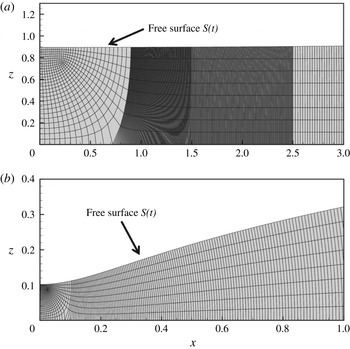
The free surface flow comprised of the transient system of partial differential equations (2.1)–(2.2) and the aforementioned boundary and initial conditions is solved numerically using a fully implicit, method of lines, arbitrary Lagrangian–Eulerian algorithm where the Galerkin/finite-element method is employed for spatial discretization (Feng & Basaran Reference Feng and Basaran1994) and an adaptive finite-difference method is used for time integration (Wilkes, Phillips & Basaran Reference Wilkes, Phillips and Basaran1999; Notz & Basaran Reference Notz and Basaran2004). As we have used variants of this algorithm to successfully analyse hydrodynamic singularities that arise in the breakup and coalescence of drops and/or filaments of both Newtonian and non-Newtonian fluids (Chen, Notz & Basaran Reference Chen, Notz and Basaran2002; Suryo & Basaran Reference Suryo and Basaran2006; Bhat et al. Reference Bhat, Appathurai, Harris, Pasquali, Mckinley and Basaran2010; Paulsen et al. Reference Paulsen, Burton, Nagel, Appathuri, Harris and Basaran2012; Collins et al. Reference Collins, Sambath, Harris and Basaran2013; Castrejón-Pita et al. Reference Castrejón-Pita, Castrejón-Pita, Thete, Sambath, Hutchings, Hinch, Lister and Basaran2015; Munro et al. Reference Munro, Anthony, Basaran and Lister2015), the reader is referred to these previous publications for details of the solution method used and computer implementation. A distinguished feature of the present and similar algorithms used in the aforementioned publications is the highly adaptive finite-element meshes that are generated using the method of elliptic mesh generation (Christodoulou & Scriven Reference Christodoulou and Scriven1992; Notz & Basaran Reference Notz and Basaran2004). A coarse version of such meshes that has been used in the simulations is shown in figure 8 where the elements and hence the mesh points are seen to concentrate near the rupture zone.
Close-up views of an illustrative coarse two-dimensional finite-element mesh that has been constructed by elliptic mesh generation for 2-D simulations. As the length of the domain in the lateral direction is 10 000, only the mesh in the vicinity of
 $h_{min}$
is shown. The two parts of the figure show the mesh (a) at the initial instant when
 $h_{min}=0.9$
and (b) at a later time when
 $h_{min}=0.1$
. The algorithm concentrates the elements more and more in the region close to the space–time singularity as the film thins and tends toward rupture.

Scaling behaviour of variables in the rupture zone during thinning of a Newtonian film of
 $Oh=1.18$
and
 $A^{\ast }=7.37\times 10^{-7}$
undergoing line rupture: simulations (data points) and scaling theory predictions (straight lines with indicated dependencies on time remaining until rupture
 $\unicode[STIX]{x1D70F}$
). Variation with
 $\unicode[STIX]{x1D70F}$
of (a) minimum film thickness
 $h_{min}$
, (b) curvature
 $\unicode[STIX]{x1D705}$
evaluated at the lateral location of
 $h_{min}$
, (c) lateral velocity
 $u^{\prime }$
evaluated at lateral location where
 $h=1.05h_{min}$
and (d) modified Reynolds number
 $Re^{\ast }$
evaluated at that lateral location.

Effect of power-law rheology on the scaling behaviour of variables in the rupture zone during thinning of a power-law film undergoing line rupture: simulations (data points) and scaling theory predictions (straight lines with indicated dependencies on time remaining until rupture
 $\unicode[STIX]{x1D70F}$
). Here,
 $Oh=1.18$
,
 $A^{\ast }=7.37\times 10^{-7}$
and
 $n=0.83$
. Variation with
 $\unicode[STIX]{x1D70F}$
of (a) minimum film thickness
 $h_{min}$
, (b) curvature
 $\unicode[STIX]{x1D705}$
evaluated at the lateral location of
 $h_{min}$
, (c) lateral velocity
 $u^{\prime }$
evaluated at lateral location where
 $h=1.05h_{min}$
and (d) modified Reynolds number
 $Re^{\ast }$
evaluated at that lateral location.

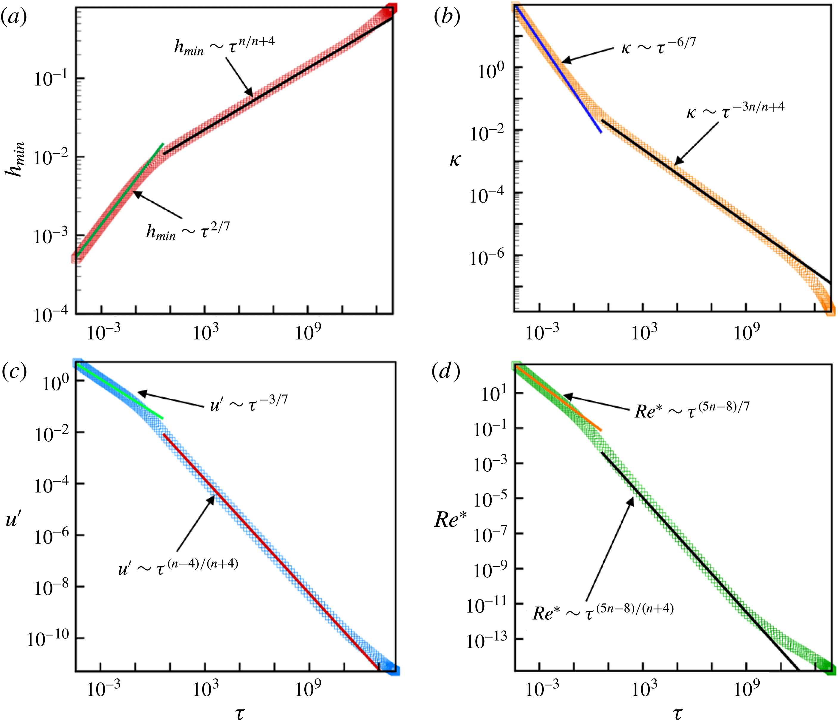
Effect of power-law rheology on the scaling behaviour of variables in the rupture zone and change of scaling during thinning of a power-law film of
 $Oh=1.18$
,
 $A^{\ast }=7.37\times 10^{-7}$
and
 $n=0.60$
undergoing line rupture: simulations (data points) and scaling theory predictions (straight lines with indicated dependencies on time remaining until rupture
 $\unicode[STIX]{x1D70F}$
). Variation with
 $\unicode[STIX]{x1D70F}$
of (a) minimum film thickness
 $h_{min}$
, (b) curvature
 $\unicode[STIX]{x1D705}$
evaluated at the lateral location of
 $h_{min}$
, (c) lateral velocity
 $u^{\prime }$
evaluated at lateral location where
 $h=1.05h_{min}$
and (d) modified Reynolds number
 $Re^{\ast }$
evaluated at that lateral location. The occurrence of a change of scaling and a transition from the viscous regime to the inertial regime is clear as
 $\unicode[STIX]{x1D70F}\rightarrow 0$
from the plots depicting the temporal evolution of all four variables in the figure.

8 Results for two-dimensional simulations with inertia
In this section, all the results that are reported have been obtained using the 2-D algorithm based on the finite-element method that is described in the previous section. The section begins by presenting results on the thinning of a Newtonian film to benchmark the 2-D algorithm and demonstrate the accuracy of predictions made with it. Thereafter, a set of results are presented for successively smaller values of
 $n$
to highlight the thinning dynamics of films of power-law liquids. The simulation results to be reported have been obtained using an initial perturbation to the film surface having an amplitude of 0.1 and wavelength of
 $4\unicode[STIX]{x03C0}h_{0}/d$
.
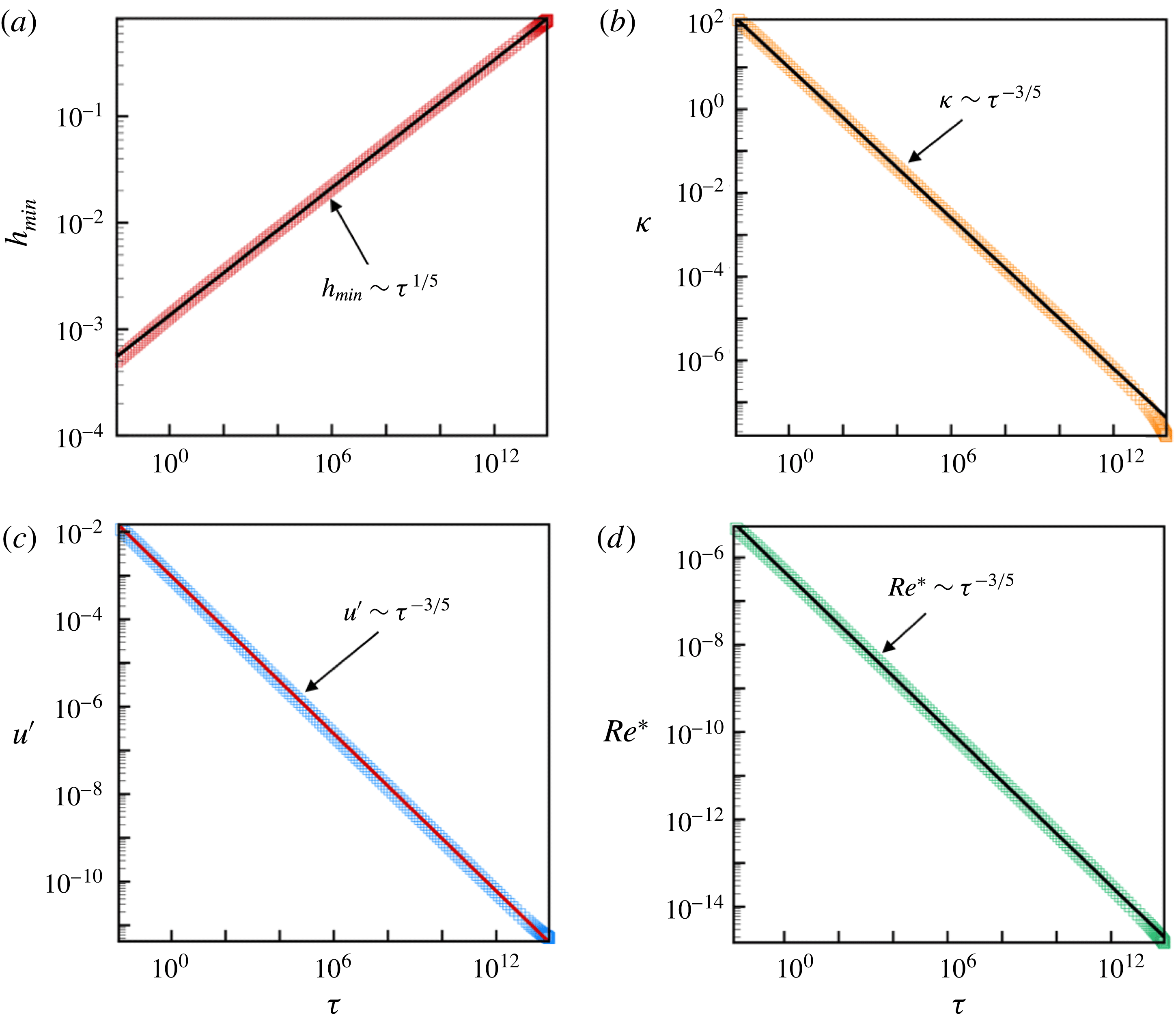
Figure 9 shows the variation with time remaining until rupture
 $\unicode[STIX]{x1D70F}$
of several quantities of interest in the rupture zone for a Newtonian film of
 $Oh=1.18$
and
 $A^{\ast }=7.37\times 10^{-7}$
. The simulation results depicted in figure 9(a) show that the minimum film thickness
 $h_{min}$
decreases with
 $\unicode[STIX]{x1D70F}$
as
 $h_{min}\sim \unicode[STIX]{x1D70F}^{1/5}$
. Figure 9(b) shows the curvature evaluated at the lateral location where the film thickness is a minimum,
 $h_{min}$
, diverges with
 $\unicode[STIX]{x1D70F}$
as
 $\unicode[STIX]{x1D705}\sim \unicode[STIX]{x1D70F}^{-3/5}$
. As has already been shown previously by (4.14), the variation of
 $\unicode[STIX]{x1D705}$
with
 $\unicode[STIX]{x1D70F}$
can be combined with the corresponding result for
 $h$
to infer that the lateral length scales as
 $x^{\prime }\sim \unicode[STIX]{x1D70F}^{2/5}$
. Figure 9(c) shows that the lateral velocity
 $u^{\prime }$
computed at the film’s surface at the lateral location where
 $h=1.05h_{min}$
diverges with
 $\unicode[STIX]{x1D70F}$
as
 $u^{\prime }\sim \unicode[STIX]{x1D70F}^{-3/5}$
. Reassuringly, this scaling result is unchanged if the lateral location at which
 $u^{\prime }$
is evaluated is changed: for example, the scaling exponent for
 $u^{\prime }$
is unchanged if
 $u^{\prime }$
is evaluated at
 $1.1h_{min}$
instead of
 $1.05h_{min}$
. Figure 9(d) shows that the modified Reynold’s number
 $Re^{\ast }$
computed at the lateral location where
 $u^{\prime }$
is evaluated to diverge with
 $\unicode[STIX]{x1D70F}$
as
 $Re^{\ast }\sim \unicode[STIX]{x1D70F}^{-3/5}$
. However, as shown in figure 9(d), the value of the modified Reynolds number remains small or
 $Re^{\ast }\ll 1$
all the way until rupture. Thus, all of the 2-D simulation results reported for the Newtonian film of this paragraph are in excellent agreement with the predictions obtained from an analysis based on the 1-D lubrication equations (cf. (4.7) and (4.8)), which is to be expected since the lubrication approximation is valid during the entire period of thinning of a Newtonian film having the properties for which the 2-D simulations have been carried out (see figure 7).
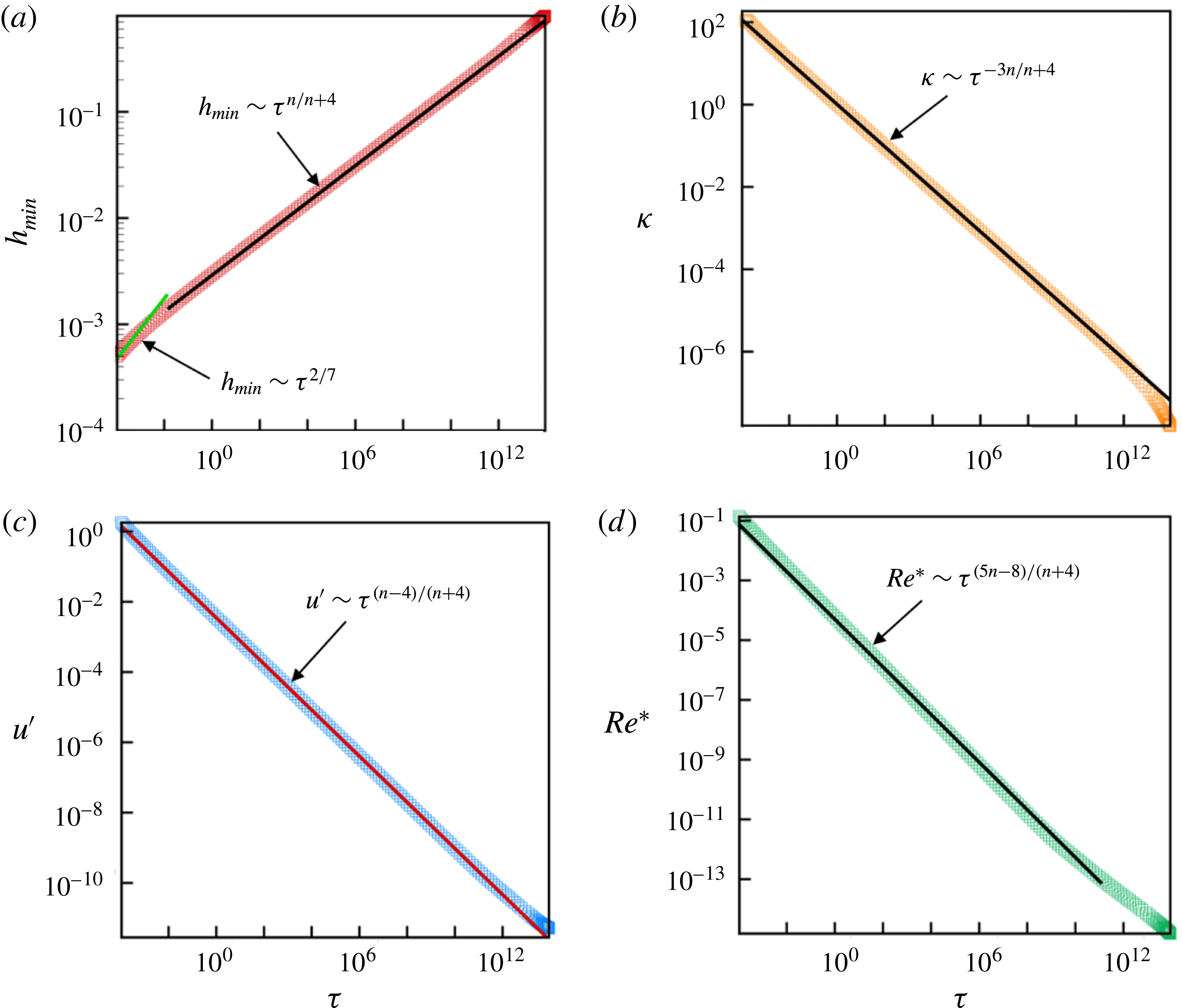
Figure 10 shows results of 2-D simulations for the thinning of a power-law film of
 $n=0.83$
and for which all the other conditions are identical to the Newtonian case discussed in the previous paragraph. For the power-law film, the simulations reveal that during virtually the entire period of thinning, the minimum film thickness, the curvature at the location where the film thickness is a minimum and the lateral velocity all follow the power-law scalings predicted by lubrication theory, viz.
 $h_{min}\sim \unicode[STIX]{x1D70F}^{n/(n+4)}\mid _{n=0.83}\sim \unicode[STIX]{x1D70F}^{0.172}$
(figure 10
a),
 $\unicode[STIX]{x1D705}\sim \unicode[STIX]{x1D70F}^{-3n/(n+4)}\mid _{n=0.83}\sim \unicode[STIX]{x1D70F}^{0.515}$
(figure 10
b) and
 $u^{\prime }\sim \unicode[STIX]{x1D70F}^{(n-4)/(n+4)}\mid _{n=0.83}\sim \unicode[STIX]{x1D70F}^{-0.656}$
(figure 10
c), because the modified Reynolds number
 $Re^{\ast }$
remains well below
 $O(1)$
(figure 10
d) until
 $h_{min}$
has decreased by three orders of magnitude. As inertia begins to become important during the final stages of thinning, the scaling exponent obtained from 2-D simulations for the variation of
 $h_{min}$
with
 $\unicode[STIX]{x1D70F}$
transitions from a value of
 $n/(n+4)=0.172$
to
 $2/7$
, as shown in figure 10(a). To see this transition from a viscous power-law regime to an inertial regime more clearly, we next consider a case for a smaller value of
 $n$
and for which the transition is expected to occur for a value of
 $h_{min}$
that is much larger than that in figure 10(a).
Figure 11 shows results of 2-D simulations for the thinning of a power-law film of
 $n=0.6$
for which all the other conditions are identical to the case of the power-law film of
 $n=0.83$
discussed in the previous paragraph (figure 10). The results depicted in figure 11(a) unequivocally show that a change of scaling occurs as the film thins such that the dynamics transitions from the viscous regime where
 $h_{min}\sim \unicode[STIX]{x1D70F}^{n/(n+4)}\mid _{n=0.60}\sim \unicode[STIX]{x1D70F}^{0.130}$
to the inertial regime that is independent of the power-law index and where
 $h_{min}\sim \unicode[STIX]{x1D70F}^{2/7}$
. According to the simulation results depicted in figure 11(a), this transition occurs when
 $h_{min}\approx 10^{-2}$
, a result that is in good agreement with the theoretical estimate of
 $h_{min}\sim 4\times 10^{-2}$
predicted by (6.6). Figure 11(b,c) make plain the changes in scaling that are exhibited by the curvature at the location where the film thickness is a minimum and the lateral velocity as the power-law film thins. The scaling exponents before and after the change of scaling predicted from the simulations are in excellent agreement with those given by (4.8) and (7.1). That inertia becomes significant as the film thins and approaches rupture is made evident from figure 11(d): this figure shows that the modified Reynolds number increases monotonically as the thinning continues and becomes
 $O(1)$
, signalling the transition from the viscous to the inertial regime. Using the expressions for the scaling estimates given by (7.1) for the variation of the film thickness, lateral length scale, and lateral velocity with
 $\unicode[STIX]{x1D70F}$
, the modified Reynolds number in the inertial regime can be shown to vary with time remaining until rupture as
 $Re^{\ast }\sim \unicode[STIX]{x1D70F}^{(5n-8)/7}$
. The modified Reynolds number predicted from simulations and that is plotted in figure 11(d) can be seen to be in excellent agreement with the theoretical scaling estimates that
 $Re^{\ast }\sim \unicode[STIX]{x1D70F}^{(5n-8)/(n+4)}$
at early times when the dynamics is in the viscous regime and that
 $Re^{\ast }\sim \unicode[STIX]{x1D70F}^{(5n-8)/7}$
at late times when the dynamics is in the inertial regime.
9 Conclusion
In this paper, the van der Waals force-driven thinning and rupture films of power-law fluids lying on a solid substrate have been analysed by two different means. When the film fluid is Newtonian (for which the power-law index
 $n=1$
) or the film is a deformation-rate-thinning fluid of power-law index that is close to one, the dynamics has been analysed by solving a spatially one-dimensional, nonlinear evolution equation that results by application of the lubrication approximation. In such situations, the dynamics has been studied both theoretically and numerically for both two-dimensional or line rupture as well as axisymmetric or point rupture. In both cases, the dynamics in the vicinity of the rupture singularity has been shown to be self-similar and for which the film thickness and the lateral length scale decrease as
 $\unicode[STIX]{x1D70F}^{n/n+4}$
and
 $\unicode[STIX]{x1D70F}^{2n/n+4}$
, respectively, where
 $\unicode[STIX]{x1D70F}$
is the dimensionless time remaining until rupture. During the thinning of such films, van der Waals, capillary (surface tension) and viscous forces remain in balance but inertia is negligible as the film tends toward rupture.
For power-law fluids of sufficiently small
 $n$
, inertia can become important once the minimum film thickness falls below a critical value. The critical conditions for which inertia becomes important and the lubrication approximation is no longer valid have been determined analytically and a phase diagram has been constructed that depicts when inertia will become important during film thinning for fluids of any value of the power-law index
 $n$
(
 $0<n\leqslant 1$
). To analyse film thinning and rupture when inertia may be important, a computational fluid dynamics (CFD) algorithm has been developed for solving the free boundary problem comprised of the transient, spatially two-dimensional Cauchy momentum and continuity equations. In situations where inertia is important, the film thickness and the lateral length scale have been shown to decrease as
 $\unicode[STIX]{x1D70F}^{2/7}$
and
 $\unicode[STIX]{x1D70F}^{4/7}$
. During the thinning of such films, van der Waals, capillary and inertial forces remain in balance but viscous force is negligible as the film tends toward rupture.
It is highly challenging to study hydrodynamic singularities that arise in free surface flows involving breakup such as thread pinch off (Eggers Reference Eggers1993) and film rupture (Zhang & Lister Reference Zhang and Lister1999) using a multidimensional CFD algorithm rather than reduced-order or one-dimensional long-wavelength models given the multiscale nature of such problems. Although multidimensional CFD algorithms had previously been used to study pinch off of fluid threads (Wilkes et al. Reference Wilkes, Phillips and Basaran1999; Chen et al. Reference Chen, Notz and Basaran2002; Suryo & Basaran Reference Suryo and Basaran2006; Collins et al. Reference Collins, Sambath, Harris and Basaran2013; Castrejón-Pita et al. Reference Castrejón-Pita, Castrejón-Pita, Thete, Sambath, Hutchings, Hinch, Lister and Basaran2015; Li & Sprittles Reference Li and Sprittles2016), to our knowledge, the present paper is the first to tackle film rupture using such an approach.
In the 2-D simulations carried out in this paper, the entire domain is discretized into a set of curved quadrilateral elements. Solving the set of spatially two-dimensional partial differential equations (PDEs) governing film thinning and rupture is costly because a large number of elements or mesh points must be used in the lateral direction as the lateral extent of the film or the maximum value of the
 $x$
-coordinate,
 $\unicode[STIX]{x1D706}/2$
, is three to five orders of magnitude larger than the undisturbed film thickness. Since the lateral velocity and the local Reynolds number decrease as one moves away from the rupture zone, an efficient computational scheme can be developed by dividing the domain into two parts: in the first part, for
 $0\leqslant x\leqslant L$
, with
 $x^{\prime }\ll L\ll \unicode[STIX]{x1D706}/2$
, and where inertia may be important, the domain is discretized into a set of 2-D quadrilateral elements and the set of spatially 2-D PDEs is solved and in the second part, for
 $L\leqslant x\leqslant \unicode[STIX]{x1D706}/2$
and where inertia is insignificant, the domain is discretized into a set of 1-D elements and the spatially 1-D long-wavelength, or lubrication, equation is solved. The lateral location
 $L$
where the two solutions are matched can be varied to minimize the error in the solution obtained with the hybrid algorithm compared to that obtained with the more expensive 2-D algorithm alone. We leave the implementation of such a hybrid algorithm as a future goal of research on studies of the thinning and rupture of thin films on substrates.
As pointed out by Witelski & Bernoff (Reference Witelski and Bernoff1999) and Zhang & Lister (Reference Zhang and Lister1999) for Newtonian fluids, two-dimensional or line rupture is unstable to perturbations in film thickness in the third direction. Since axisymmetric solutions are stable with respect to asymmetric perturbations, unstable thin films are generally expected to rupture at a point.
Acknowledgements
The authors thank the Petroleum Research Fund of the American Chemical Society (ACS/PRF), the Purdue Process Safety and Assurance Center (P2SAC), the Dean’s Office in the College of Engineering at Purdue University, and the Burton and Kathryn Gedge Professorship to O.A.B. for financial support.
Appendix A. Governing equations in the lubrication limit
When the divergence of the stress tensor is evaluated, the Cauchy momentum equation can be rewritten as
 $$\begin{eqnarray}\unicode[STIX]{x1D70C}\left(\frac{\unicode[STIX]{x2202}\tilde{\boldsymbol{v}}}{\unicode[STIX]{x2202}\tilde{t}}+\tilde{\boldsymbol{v}}\boldsymbol{\cdot }\tilde{\unicode[STIX]{x1D735}}\tilde{\boldsymbol{v}}\right)=-\tilde{\unicode[STIX]{x1D735}}\tilde{p}+\tilde{\unicode[STIX]{x1D707}}\tilde{\unicode[STIX]{x1D6FB}}^{2}\tilde{\boldsymbol{v}}+\tilde{\unicode[STIX]{x1D735}}\tilde{\unicode[STIX]{x1D707}}\boldsymbol{\cdot }\tilde{\unicode[STIX]{x1D735}}\tilde{\boldsymbol{v}}+\tilde{\unicode[STIX]{x1D735}}\tilde{\boldsymbol{v}}\boldsymbol{\cdot }\tilde{\unicode[STIX]{x1D735}}\tilde{\unicode[STIX]{x1D707}}.\end{eqnarray}$$
In what follows, it proves convenient to decompose the fluid velocity and the gradient operator into two parts, one of which is parallel to the solid substrate and the other perpendicular to it, viz.
 $$\begin{eqnarray}\tilde{\boldsymbol{v}}=\tilde{\boldsymbol{v}}_{H}+\tilde{w},\quad \tilde{\unicode[STIX]{x1D735}}=\tilde{\unicode[STIX]{x1D735}}_{H}+\boldsymbol{e}_{z}\frac{\unicode[STIX]{x2202}}{\unicode[STIX]{x2202}\tilde{z}}.\end{eqnarray}$$
With these definitions, the continuity equation and the components of the Cauchy momentum equation in the direction parallel and perpendicular to the substrate can be written as
 $$\begin{eqnarray}\tilde{\unicode[STIX]{x1D735}}_{H}\boldsymbol{\cdot }\tilde{\boldsymbol{v}}_{H}+\frac{\unicode[STIX]{x2202}\tilde{w}}{\unicode[STIX]{x2202}\tilde{z}}=0,\end{eqnarray}$$
 $$\begin{eqnarray}\displaystyle \unicode[STIX]{x1D70C}\left(\frac{\unicode[STIX]{x2202}\tilde{\boldsymbol{v}}_{H}}{\unicode[STIX]{x2202}\tilde{t}}+\tilde{\boldsymbol{v}}_{H}\boldsymbol{\cdot }\tilde{\unicode[STIX]{x1D735}}_{H}\tilde{\boldsymbol{v}}_{H}+\tilde{w}\frac{\unicode[STIX]{x2202}\tilde{\boldsymbol{v}}_{H}}{\unicode[STIX]{x2202}\tilde{z}}\right) & = & \displaystyle -\tilde{\unicode[STIX]{x1D735}}_{H}\tilde{p}+\tilde{\unicode[STIX]{x1D707}}\left(\tilde{\unicode[STIX]{x1D6FB}}_{H}^{2}\tilde{\boldsymbol{v}}_{H}+\frac{\unicode[STIX]{x2202}^{2}\tilde{\boldsymbol{v}}_{H}}{\unicode[STIX]{x2202}\tilde{z}^{2}}\right)\nonumber\\ \displaystyle & & \displaystyle +\,\tilde{\unicode[STIX]{x1D735}}_{H}\tilde{\unicode[STIX]{x1D707}}\boldsymbol{\cdot }\tilde{\unicode[STIX]{x1D735}}_{H}\tilde{\boldsymbol{v}}_{H}+\frac{\unicode[STIX]{x2202}\tilde{\unicode[STIX]{x1D707}}}{\unicode[STIX]{x2202}\tilde{z}}\,\frac{\unicode[STIX]{x2202}\tilde{\boldsymbol{v}}_{H}}{\unicode[STIX]{x2202}\tilde{z}}\nonumber\\ \displaystyle & & \displaystyle +\,\tilde{\unicode[STIX]{x1D735}}_{H}\tilde{\boldsymbol{v}}_{H}\boldsymbol{\cdot }\tilde{\unicode[STIX]{x1D735}}_{H}\tilde{\unicode[STIX]{x1D707}}+\frac{\unicode[STIX]{x2202}\tilde{\unicode[STIX]{x1D707}}}{\unicode[STIX]{x2202}\tilde{z}}\tilde{\unicode[STIX]{x1D735}}_{H}\tilde{w},\end{eqnarray}$$
 $$\begin{eqnarray}\displaystyle \unicode[STIX]{x1D70C}\left(\frac{\unicode[STIX]{x2202}\tilde{w}}{\unicode[STIX]{x2202}\tilde{t}}+\tilde{\boldsymbol{v}}_{H}\boldsymbol{\cdot }\tilde{\unicode[STIX]{x1D735}}_{H}\tilde{w}+\tilde{w}\frac{\unicode[STIX]{x2202}\tilde{w}}{\unicode[STIX]{x2202}\tilde{z}}\right) & = & \displaystyle -\frac{\unicode[STIX]{x2202}\tilde{p}}{\unicode[STIX]{x2202}\tilde{z}}+\tilde{\unicode[STIX]{x1D707}}\left(\tilde{\unicode[STIX]{x1D6FB}}_{H}^{2}\tilde{w}+\frac{\unicode[STIX]{x2202}^{2}\tilde{w}}{\unicode[STIX]{x2202}\tilde{z}^{2}}\right)\nonumber\\ \displaystyle & & \displaystyle +\,\tilde{\unicode[STIX]{x1D735}}_{H}\tilde{\unicode[STIX]{x1D707}}\boldsymbol{\cdot }\tilde{\unicode[STIX]{x1D735}}_{H}\tilde{w}+2\frac{\unicode[STIX]{x2202}\tilde{\unicode[STIX]{x1D707}}}{\unicode[STIX]{x2202}\tilde{z}}\frac{\unicode[STIX]{x2202}\tilde{w}}{\unicode[STIX]{x2202}\tilde{z}}+\frac{\unicode[STIX]{x2202}\tilde{\boldsymbol{v}}_{H}}{\unicode[STIX]{x2202}\tilde{z}}\boldsymbol{\cdot }\tilde{\unicode[STIX]{x1D735}}_{H}\tilde{\unicode[STIX]{x1D707}}.\end{eqnarray}$$
In thin film flow, the characteristic length scale in the vertical direction,
 $h_{0}$
, is much smaller than that in the horizontal or lateral direction,
 $l_{c}$
, so that the aspect ratio or slenderness of the film
 $\unicode[STIX]{x1D716}\equiv h_{0}/l_{c}\ll 1$
. It then follows from the continuity equation (A 3) that if the characteristic velocity scales in the horizontal and vertical directions are given by
 $u_{c}$
and
 $w_{c}$
, then
 $w_{c}\sim \unicode[STIX]{x1D716}u_{c}$
. If the characteristic time, pressure and viscosity scales are taken to be
 $t_{c}=l_{c}/u_{c}$
,
 $p_{c}=\unicode[STIX]{x1D707}_{0}u_{c}l_{c}/h_{0}^{2}$
and
 $\unicode[STIX]{x1D707}_{0}$
, the continuity equation and the lateral and axial components of the Cauchy momentum equation in dimensionless form become
 $$\begin{eqnarray}\unicode[STIX]{x1D735}_{H}\boldsymbol{\cdot }\boldsymbol{v}_{H}+\frac{\unicode[STIX]{x2202}w}{\unicode[STIX]{x2202}z}=0,\end{eqnarray}$$
 $$\begin{eqnarray}\displaystyle Re\,\unicode[STIX]{x1D716}\left(\frac{\unicode[STIX]{x2202}\boldsymbol{v}_{H}}{\unicode[STIX]{x2202}t}+\boldsymbol{v}_{H}\boldsymbol{\cdot }\unicode[STIX]{x1D735}_{H}\boldsymbol{v}_{H}+w\frac{\unicode[STIX]{x2202}\boldsymbol{v}_{H}}{\unicode[STIX]{x2202}z}\right) & = & \displaystyle -\unicode[STIX]{x1D735}_{H}p+\unicode[STIX]{x1D707}\left(\unicode[STIX]{x1D716}^{2}\unicode[STIX]{x1D6FB}_{H}^{2}\boldsymbol{v}_{H}+\frac{\unicode[STIX]{x2202}^{2}\boldsymbol{v}_{H}}{\unicode[STIX]{x2202}z^{2}}\right)+\frac{\unicode[STIX]{x2202}\unicode[STIX]{x1D707}}{\unicode[STIX]{x2202}z}\frac{\unicode[STIX]{x2202}\boldsymbol{v}_{H}}{\unicode[STIX]{x2202}z}\nonumber\\ \displaystyle & & \displaystyle +\,\unicode[STIX]{x1D716}^{2}\left(\unicode[STIX]{x1D735}_{H}\unicode[STIX]{x1D707}\boldsymbol{\cdot }\unicode[STIX]{x1D735}_{H}\boldsymbol{v}_{H}+\unicode[STIX]{x1D735}_{H}\boldsymbol{v}_{H}\boldsymbol{\cdot }\unicode[STIX]{x1D735}_{H}\unicode[STIX]{x1D707}+\frac{\unicode[STIX]{x2202}\unicode[STIX]{x1D707}}{\unicode[STIX]{x2202}z}\unicode[STIX]{x1D735}_{H}w\right)\!,\hspace{-10.00002pt}\nonumber\\ \displaystyle & & \displaystyle\end{eqnarray}$$
 $$\begin{eqnarray}\displaystyle Re\,\unicode[STIX]{x1D716}\left(\frac{\unicode[STIX]{x2202}w}{\unicode[STIX]{x2202}t}+\boldsymbol{v}_{H}\boldsymbol{\cdot }\unicode[STIX]{x1D735}_{H}w+w\frac{\unicode[STIX]{x2202}w}{\unicode[STIX]{x2202}z}\right) & = & \displaystyle -\frac{1}{\unicode[STIX]{x1D716}^{2}}\frac{\unicode[STIX]{x2202}p}{\unicode[STIX]{x2202}z}+\unicode[STIX]{x1D707}\left(\unicode[STIX]{x1D716}^{2}\unicode[STIX]{x1D6FB}_{H}^{2}w+\frac{\unicode[STIX]{x2202}^{2}w}{\unicode[STIX]{x2202}z^{2}}\right)\nonumber\\ \displaystyle & & \displaystyle +\,\unicode[STIX]{x1D735}_{H}\unicode[STIX]{x1D707}\boldsymbol{\cdot }\left(\unicode[STIX]{x1D716}^{2}\unicode[STIX]{x1D735}_{H}w+\frac{\unicode[STIX]{x2202}\boldsymbol{v}_{H}}{\unicode[STIX]{x2202}z}\right)+2\frac{\unicode[STIX]{x2202}\unicode[STIX]{x1D707}}{\unicode[STIX]{x2202}z}\frac{\unicode[STIX]{x2202}w}{\unicode[STIX]{x2202}z},\end{eqnarray}$$
where
 $Re=\unicode[STIX]{x1D70C}u_{c}h_{0}/\unicode[STIX]{x1D707}_{0}$
is the Reynolds number and variables that appear without tildes over them are the dimensionless counterparts of those with tildes. Equations similar to equations (A 6), (A 7) and (A 8), albeit for Newtonian fluids and typically with lateral variation in a single direction, can be found in standard books in fluid mechanics and transport phenomena (cf. Deen (Reference Deen1998)). In the lubrication approximation, both the aspect ratio and the Reynolds number times aspect ratio must be small, viz.
 $\unicode[STIX]{x1D716}\ll 1$
and
 $Re\,\unicode[STIX]{x1D716}\ll 1$
.