1 Introduction
At low angle of attack, the flow past a translating wing is attached, generating a steady lift. This attached flow regime is the preferred one for conventional aircraft. At high angle of attack, above the critical static stall angle, the flow separates at the leading edge and rolls up into a leading edge vortex (LEV). In the absence of three-dimensional effects, and above a critical Reynolds number, this LEV is unstable in the sense that it is shed into the wake at some point. On the contrary, at similar high angle of attack and similar Reynolds number, the LEV can be stabilized under the influence of three-dimensional effects. It has been shown that three-dimensional effects arising from the tip condition significantly affect the separated flow over a portion of the wing roughly extending from the wing tip to approximately 1.5 chords away from it (Ringuette, Milano & Gharib Reference Ringuette, Milano and Gharib2007; Jardin, Farcy & David Reference Jardin, Farcy and David2012) and that the LEV can be stabilized on low aspect ratio wings where these three-dimensional effects become prominent (Taira & Colonius Reference Taira and Colonius2009).
In the case of a rotating wing, it is known that the LEV can reach a stable state for higher aspect ratios than those ensuring LEV stability on a translating wing (e.g. Kruyt et al. Reference Kruyt, van Heijst, Altshuler and Lentink2015). That is, some other three-dimensional effects than those arising from the tip condition must be responsible for LEV stability. These three-dimensional effects may arise from (i) spanwise gradients in wing speed and (ii) rotational accelerations.
Spanwise gradients in wing speed are responsible for the development of a spanwise flow in the core of the LEV (Jardin & David Reference Jardin and David2014). Through an analogy with mechanisms of LEV stabilization on Delta wings, Ellington et al. (Reference Ellington, Van den Berg, Willmott and Thomas1996) and van den Berg & Ellington (Reference van den Berg and Ellington1997) suggest that the resulting spanwise flow tends to drain vorticity out of the LEV core, hence balancing the production of vorticity at the leading edge and preventing the LEV from reaching a critical size that would trigger its shedding. Various studies explore this hypothesis using translating swept wings (Lentink & Dickinson Reference Lentink and Dickinson2009; Beem, Rival & Triantafyllou Reference Beem, Rival and Triantafyllou2012). In such cases, the oncoming flow has a velocity component that is collinear to the LEV axis, potentially contributing to vorticity drainage towards the wing tip. The collinear velocity component increases as the sweep angle increases, suggesting that high sweep angles are conducive to LEV attachment. Nonetheless, experiments reported by Lentink & Dickinson (Reference Lentink and Dickinson2009) and Beem et al. (Reference Beem, Rival and Triantafyllou2012) demonstrate that the LEV is shed after a short distance of travel, even for high sweep angles. Thus, the analogy introduced by Ellington et al. (Reference Ellington, Van den Berg, Willmott and Thomas1996) and van den Berg & Ellington (Reference van den Berg and Ellington1997) to explain stable LEV attachment on revolving wings is not strictly valid. This is not to say that spanwise flow has no influence on LEV attachment. Recently, Jardin & David (Reference Jardin and David2014) explore the hypothesis under a new perspective. The authors analyse the LEV that develops on a wing embedded in a spanwise varying oncoming flow. They show that the attachment of the LEV is promoted by the spanwise flow that develops due to spanwise gradients in wing speed, but that the LEV still tends to deviate from a stable state.
Therefore, it is believed that LEV stabilization on revolving wings derives from rotational accelerations. Lentink & Dickinson (Reference Lentink and Dickinson2009) first formulated this hypothesis, suggesting that the Rossby number is the relevant scaling parameter to describe LEV stability. Recent work by Wolfinger & Rockwell (Reference Wolfinger and Rockwell2014) provides a detailed investigation on the relationship between the LEV structure and the Rossby number. Together with general observations made by Kruyt et al. (Reference Kruyt, van Heijst, Altshuler and Lentink2015), findings by Wolfinger & Rockwell (Reference Wolfinger and Rockwell2014) support the hypothesis that rotational accelerations mediate LEV stability on revolving wings. Moreover, by numerically solving the Navier–Stokes equations in the non-inertial reference frame of the wing, with and without Coriolis and centrifugal terms, Jardin & David (Reference Jardin and David2015) further suggest that the Coriolis effect is the key ingredient in LEV stability.
Building on this last hypothesis, the present paper clarifies the role of the Coriolis acceleration on the attachment of the LEV. Numerical simulations of the flow past high angle of attack revolving wings are performed for different Reynolds numbers, with the Coriolis acceleration being artificially reduced or increased in the Navier–Stokes equations. A relatively high aspect ratio (9.5) is considered to allow identifying the spanwise transition of the LEV from a stable to an unstable state in the absence of any significant tip effects, which is different to most bio-oriented studies that usually consider low aspect ratio wings, as found in nature. This set-up ultimately leads to a quantified relationship between the spanwise location of the transition of the LEV from a stable to an unstable state and the strength of the Coriolis acceleration. Along with the analysis of relevant flow quantities, such as spanwise velocities and pressure gradients, this quantification provides insight into the mechanisms that drive the attachment of the LEV on revolving wings. Because a relatively high aspect ratio is considered, the results have outcomes that go beyond the scope of bio-inspired flight and can help defining enhanced low-order models (e.g. blade element models) taking into account rotational effects or open the path towards the definition of new control strategies that mimic Coriolis effect to delay stall.
2 Problem set-up
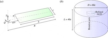
The problem consists of a finite-span rectangular planform wing that impulsively rotates about an axis that is perpendicular to its span and that intersects the spanwise wing axis located at mid-chord (figure 1 a).
Geometrical parameters of the rotating wing (a) and computational domain (b). Not scaled for the sake of clarity.

The wing has a radius
 $R=10c$
and an aspect ratio
 $AR=b/c=(R-rco)/c=9.5$
, where
 $c$
,
 $b$
and
 $rco$
are the lengths of the wing chord, wing span and root cutout respectively (figure 1
a). The wing profile is a 4 % thickness flat plate with sharp leading and trailing edges. Unless otherwise indicated, the wing rotates through a revolution angle
 $\unicode[STIX]{x1D719}=180^{\circ }$
at an angle of attack
 $\unicode[STIX]{x1D6FC}=45^{\circ }$
, far beyond the static stall angle of the profile (cases with
 $\unicode[STIX]{x1D6FC}=15^{\circ }$
and
 $\unicode[STIX]{x1D6FC}=30^{\circ }$
are also briefly addressed). It produces a thrust,
 $T$
, and a rotational torque along the rotation axis,
 $Q$
.
The wing is embedded in a cylindrical computational domain of diameter
 $60c$
and length
 $40c$
(figure 1
b). Note that for future purposes that go beyond the scope of the present study, a cylindrical hole of diameter
 $0.25c$
runs through the domain along the rotation axis – it was verified that such a hole has a negligible influence on the results presented thereafter. The flow in the domain is computed by directly resolving the incompressible Navier–Stokes equations in the non-inertial reference frame of the wing:
 $$\begin{eqnarray}\frac{\unicode[STIX]{x2202}u}{\unicode[STIX]{x2202}t}+u\boldsymbol{\cdot }\unicode[STIX]{x1D735}u=-\frac{1}{\unicode[STIX]{x1D70C}}\unicode[STIX]{x1D735}p-\unicode[STIX]{x1D6FA}\times (\unicode[STIX]{x1D6FA}\times r)-2\unicode[STIX]{x1D6FA}\times u+\unicode[STIX]{x1D708}\unicode[STIX]{x1D6FB}^{2}u,\end{eqnarray}$$
using a finite volume method. Momentum and continuity equations are uncoupled and solved using a predictor–corrector approach. A co-located variable arrangement and a Rhie-and-Chow-type pressure–velocity coupling combined with a SIMPLE-type algorithm are used (Rhie & Chow Reference Rhie and Chow1993; Ferziger & Peric Reference Ferziger and Peric2002). Second-order schemes are employed for both spatial and temporal discretizations. The wing is modelled as a fixed non-slip surface and a velocity Dirichlet condition
 $-\unicode[STIX]{x1D6FA}\times r$
is applied on all external boundaries (including the centre hole), where
 $\unicode[STIX]{x1D6FA}$
is the wing rotation speed and
 $r$
is the radial distance from the wing axis of rotation. The Reynolds number based on the wing chord
 $c$
and the mean velocity along the wing radius
 $\unicode[STIX]{x1D6FA}R/2$
is in the range
 $Re\in [100;750]$
. Recall that in (2.1),
 $t$
,
 $\unicode[STIX]{x1D708}$
,
 $\unicode[STIX]{x1D70C}$
,
 $u$
and
 $p$
stands for the time and for the kinematic viscosity, density, velocity and pressure of the surrounding fluid respectively.
A Cartesian grid is used which consists of 25 million cells, with a typical grid spacing in all three dimensions of
 $\unicode[STIX]{x0394}s=0.02c$
in the vicinity of the wing (refined mesh region in figure 1
b). The Cartesian cells are trimmed to fit the wing and the external (cylindrical) boundaries. The time step is fixed to
 $\unicode[STIX]{x0394}t=2\unicode[STIX]{x03C0}/720\unicode[STIX]{x1D6FA}$
.
The configuration investigated here is comparable to that addressed in Jardin & David (Reference Jardin and David2014), Jardin & David (Reference Jardin and David2015) and Jardin & David (Reference Jardin and David2017). Convergence tests in Jardin & David (Reference Jardin and David2017) show that the Navier–Stokes solution of the flow past a
 $45^{\circ }$
angle of attack revolving wing at Reynolds number 500 is converged with respect to spatial and temporal resolutions for
 $\unicode[STIX]{x0394}s=0.02c$
and
 $\unicode[STIX]{x0394}t=2\unicode[STIX]{x03C0}/360\unicode[STIX]{x1D6FA}$
. For these tests, it is posited that convergence is achieved if an arbitrary increase in spatial and temporal resolutions does not induce a variation in both mean and instantaneous aerodynamic loads (both wing lift
 $L$
and torque
 $Q$
) of more than 0.5 % and 2 % respectively. Moreover, the results obtained in Jardin & David (Reference Jardin and David2017) show reasonable agreement with experimental data. Finally, it should also be mentioned that the finite volume method employed here has already proven its ability to accurately predict the occurrence of flow instabilities at low Reynolds numbers (Bury & Jardin Reference Bury and Jardin2012).
Although previous tests provide confidence in the accuracy of the present approach, and since the maximum Reynolds number addressed here is slightly higher than that addressed in these previous studies, additional tests are performed at
 $Re=750$
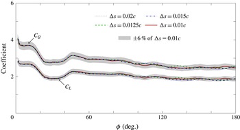
, confirming the independency of the results to both spatial and temporal resolutions. Figure 2 compares the instantaneous lift and torque coefficients obtained using the reported spatial resolution
 $\unicode[STIX]{x0394}s=0.02c$
with those obtained by increasing the total number of cells by approximately a factor of 2 (
 $\unicode[STIX]{x0394}s=0.015c$
), 4 (
 $\unicode[STIX]{x0394}s=0.0125c$
) and 8 (
 $\unicode[STIX]{x0394}s=0.01c$
). It can be seen that slight discrepancies exist for revolution angles larger than
 $\unicode[STIX]{x1D719}=90^{\circ }$
, i.e. when initial transients have decayed and a large portion of the wing, outboard, exhibits unsteady flow structures (see flow description in § 4.1.1). In all cases, the curves lie within
 $\pm 6\,\%$
bounds around the values obtained using spatial resolution
 $\unicode[STIX]{x0394}s=0.01c$
(indicated by the grey area). Moreover, the mean lift and torque coefficients obtained with
 $\unicode[STIX]{x0394}s=0.02c$
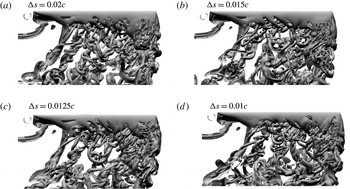
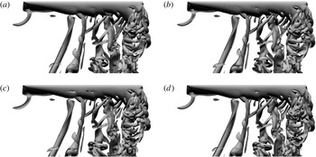
are only 1 % and 1.2 % away from the Richardson extrapolated solutions respectively (Roache Reference Roache1998). Figure 3 displays iso-surfaces of
 $q$
-criterion (see Jeong & Hussain Reference Jeong and Hussain1995) obtained for spatial resolutions corresponding to those in figure 2, at
 $\unicode[STIX]{x1D719}=180^{\circ }$
. It can be seen that the flow structure is very similar for all cases, revealing a quasi-steady flow inboard and an unsteady flow outboard (see flow description in § 4.1.1). More importantly, the frontier between quasi-steady and unsteady flows does not change with
 $\unicode[STIX]{x0394}s$
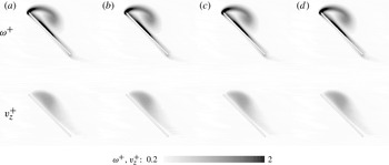
. Figure 4 shows
 $q$
-criterion iso-lines and contours of vorticity magnitude in a spanwise cross-section located in the quasi-steady region, 2 chords away from the axis of rotation. Here again, the comparison reveals negligible changes with
 $\unicode[STIX]{x0394}s$
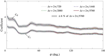
. Finally, it was verified that the reported results are converged with respect to the temporal resolution. A figure that compares the instantaneous lift and torque coefficients obtained using the reported temporal resolution
 $\unicode[STIX]{x0394}t=2\unicode[STIX]{x03C0}/720$
with those obtained by decreasing the time step by a factor of 2 (
 $\unicode[STIX]{x0394}t=2\unicode[STIX]{x03C0}/1440$
), 4 (
 $\unicode[STIX]{x0394}t=2\unicode[STIX]{x03C0}/2880$
) and 8 (
 $\unicode[STIX]{x0394}t=2\unicode[STIX]{x03C0}/5760$
) is provided in appendix A (figure 25). Here again, it is shown that the reported temporal resolution is sufficient to capture the main features of the flow with reasonable accuracy.
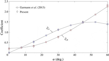
For the sake of completeness, the results obtained using the present approach (
 $\unicode[STIX]{x0394}s=0.02c$
,
 $\unicode[STIX]{x0394}t=2\unicode[STIX]{x03C0}/720$
) are compared with those obtained in Garmann, Visbal & Orkwis (Reference Garmann, Visbal and Orkwis2013) for a revolving wing with aspect ratio
 $AR=1$
and root cutout
 $rco=0.52c$
(i.e. radius
 $R=1.02c$
). The Reynolds number based on the wing speed at midspan is 500, which is within the range of
 $Re$
considered in the present paper. Figure 5 shows this comparison in terms of mean lift
 $\bar{C_{L}}$
and drag
 $\bar{C_{D}}$
coefficients over angles of attacks ranging from 0
 $^{\circ }$
to 60
 $^{\circ }$
, which encompass angles of attack tested here. Note that mean values are computed by integrating instantaneous values over revolution angles
 $\unicode[STIX]{x1D719}\in [45^{\circ }-315^{\circ }]$
. It can be seen that relatively good agreement is achieved between both approaches.
Coefficients of lift
 $C_{L}$
and torque
 $C_{Q}$
as a function of the revolution angle
 $\unicode[STIX]{x1D719}$
for different spatial resolutions
 $\unicode[STIX]{x0394}s$
.

Iso-surfaces of
 $q$
-criterion obtained at revolution angle
 $\unicode[STIX]{x1D719}=180^{\circ }$
for different spatial resolutions
 $\unicode[STIX]{x0394}s$
.

Iso-lines of
 $q$
-criterion and contours of vorticity magnitude obtained in a spanwise cross-section located 2 chords away from the axis of rotation at revolution angle
 $\unicode[STIX]{x1D719}=180^{\circ }$
for different spatial resolutions
 $\unicode[STIX]{x0394}s$
.

Mean coefficients of lift
 $\bar{C_{L}}$
and drag
 $\bar{C_{D}}$
as a function of the angle of attack
 $\unicode[STIX]{x1D6FC}$
obtained for a wing with aspect ratio 1. Comparison between results obtained using the present approach with those obtained by Garmann et al. (Reference Garmann, Visbal and Orkwis2013).

In order to unravel the role of the Coriolis effect on the flow that develops around the rotating wing, and more specifically on the attachment of the LEV, the Coriolis factor
 $F_{co}$
is introduced in the Navier–Stokes equations:
 $$\begin{eqnarray}\frac{\unicode[STIX]{x2202}u}{\unicode[STIX]{x2202}t}+u\boldsymbol{\cdot }\unicode[STIX]{x1D735}u=-\frac{1}{\unicode[STIX]{x1D70C}}\unicode[STIX]{x1D735}p-\underbrace{\unicode[STIX]{x1D6FA}F_{ce}\times (\unicode[STIX]{x1D6FA}\times r)}_{centrifugal}-\underbrace{2\unicode[STIX]{x1D6FA}F_{co}\times u}_{Coriolis}+\unicode[STIX]{x1D708}\unicode[STIX]{x1D6FB}^{2}u.\end{eqnarray}$$
Numerical simulations are performed for
 $F_{co}$
values ranging from 0.5 to 2. As such, it is possible to tune the relative strength of the Coriolis term keeping all other terms constant. Therefore, cases where
 $F_{co}\neq 0$
and
 $F_{co}\neq 1$
do not correspond to any realistic flow. They constitute the only way to analyse the influence of the Coriolis effect without changing any other flow characteritics, such as the local Reynolds number, the wing aspect ratio or the spanwise gradient in flow speed induced by the rotation. Similarly, the centrifugal factor
 $F_{ce}$
is introduced.
3 Non-dimensionalization
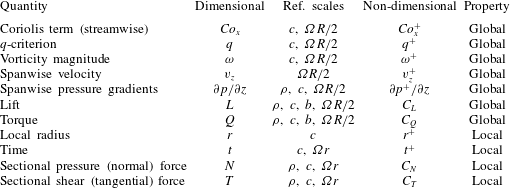
Results in the following section are analysed in terms of non-dimensional global and local quantities. Global quantities are non-dimensionalized using the wing chord
 $c$
and the mean speed along the wing radius
 $\unicode[STIX]{x1D6FA}R/2$
as reference length and velocity scales respectively. Local quantities are non-dimensionalized using the local wing chord
 $c$
and the local wing speed
 $\unicode[STIX]{x1D6FA}r$
at the corresponding spanwise cross-section of the wing. Table 1 provides an overview of these quantities.
Non-dimensionalization of the quantities used for the analysis of the results.

4 Results
4.1 Baseline case
This section focuses on the baseline case, where
 $F_{co}=1$
,
 $F_{ce}=1$
and
 $Re=\unicode[STIX]{x1D6FA}Rc/2\unicode[STIX]{x1D708}=500$
. This case corresponds to the realistic case of a wing rotating about its rotation axis.
4.1.1 Flow structure
Figure 6 shows iso-surfaces of
 $q$
-criterion at 6 instants corresponding to revolution angles
 $\unicode[STIX]{x1D719}=30^{\circ }$
,
 $60^{\circ }$
,
 $90^{\circ }$
,
 $120^{\circ }$
and
 $180^{\circ }$
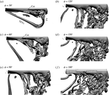
. The wing is shown from the top with the span oriented horizontally and the wing root and wing tip on the left- and right-hand side respectively. As the flow is impulsively started, a LEV, a starting trailing edge vortex (sTEV) and a tip vortex (TV) develop. While the sTEV is immediately shed and advects downstream into the wake, the LEV develops close to the wing surface during the initial stages of the wing motion. At some point, the LEV detaches in the outboard region of the wing and forms an arch-like structure that is very common to impulsively started revolving wing flows (e.g. Garmann et al.
Reference Garmann, Visbal and Orkwis2013; Harbig, Sheridan & Thompson Reference Harbig, Sheridan and Thompson2013; Venkata & Jones Reference Venkata and Jones2013; Carr, DeVoria & Ringuette Reference Carr, DeVoria and Ringuette2015; Percin & van Oudheusden Reference Percin and van Oudheusden2015). Note that, since there is no consensus on the precise definition of shedding (or detachment), shedding here refers to a cut in the
 $q$
-criterion iso-surface used to identify a specific vortex. The arch-like structure is visible in figure 6 at
 $\unicode[STIX]{x1D719}=30^{\circ }$
, which also highlights the vortex loop structure formed by the connections between the LEV, sTEV and TV. In addition, while the LEV detaches in the outboard region of the wing, it remains attached in the inboard region. It is shown that the cut in the LEV
 $q$
-criterion iso-surface occurs around midspan at
 $\unicode[STIX]{x1D719}=30^{\circ }$
but propagates towards the wing root as the revolution angle reaches
 $\unicode[STIX]{x1D719}=60^{\circ }$
. At
 $\unicode[STIX]{x1D719}=60^{\circ }$
, the LEV is shed along most of the span, except in the very inboard region. As it advects downstream, the shed LEV rotates under the effects of rotational shear (i.e. spanwise gradients in flow speed) with its inner end pinned to the wing. LEV formation and shedding is followed by TEV and secondary LEV formation and shedding. These structures evolve in a relatively similar way to that observed for the initial LEV such that the flow in the outboard region of the wing at
 $\unicode[STIX]{x1D719}=90^{\circ }$
exhibits a vortex street that is inclined with respect to the wing. In contrast to this highly unsteady pattern, the flow in the inboard region of the wing still exhibits LEV attachment. Moreover, the extent of this stable region is not significantly reduced with respect to its extent at
 $\unicode[STIX]{x1D719}=60^{\circ }$
. As such, the flow seems to have reached a limit cycle at
 $\unicode[STIX]{x1D719}=120^{\circ }$
, which is consistent with previous experimental and numerical studies (Carr et al.
Reference Carr, DeVoria and Ringuette2015; Percin & van Oudheusden Reference Percin and van Oudheusden2015; Jardin & David Reference Jardin and David2017). The flow fields at
 $\unicode[STIX]{x1D719}=120^{\circ }$
,
 $150^{\circ }$
and
 $180^{\circ }$
exhibit roughly similar patterns with (i) an unsteady outboard region and (ii) a quasi-steady inboard region. The next section aims at correlating the flow in these regions with global and sectional aerodynamic forces.
Iso-surfaces of
 $q$
-criterion (
 $q^{+}=0.25$
and 2.5) obtained at 6 revolution angles
 $\unicode[STIX]{x1D719}$
. Baseline case:
 $F_{co}=F_{ce}=1$
and
 $Re=500$
. Dash-dotted and plain lines indicate shed LEVs and TEVs respectively.

4.1.2 Global and sectional forces
Figure 7 shows the lift
 $C_{L}$
and torque
 $C_{Q}$
coefficients of the wing and the lift-to-torque coefficient ratio
 $C_{L}/C_{Q}$
as a function of the revolution angle
 $\unicode[STIX]{x1D719}$
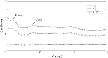
. It is observed that both
 $C_{L}$
and
 $C_{Q}$
exhibit a narrow plateau during the initial stages of the motion, which correspond to the build-up phase of the LEV. Rapid shedding of the LEV in the outboard region of the wing then leads to a drop in
 $C_{L}$
and
 $C_{Q}$
around
 $\unicode[STIX]{x1D719}=20^{\circ }$
. The subsequent valley is followed by a bump which marks the build-up of the secondary LEV observed in the outboard region of the wing. Although
 $C_{L}$
and
 $C_{Q}$
undergo a slight decrease at
 $\unicode[STIX]{x1D719}=120^{\circ }$
, they seem to stabilize near
 $\unicode[STIX]{x1D719}=60^{\circ }$
around values of the order of 2 and 3 respectively. This suggests that, although changes in the flow fields are observed from
 $\unicode[STIX]{x1D719}=60^{\circ }$
to
 $\unicode[STIX]{x1D719}=120^{\circ }$
, prominent transients have decayed around
 $\unicode[STIX]{x1D719}=60^{\circ }$
. Overall,
 $C_{L}$
and
 $C_{Q}$
have very similar trends because they derive from vortex force which applies normal to the wing surface. As a consequence, the
 $C_{L}/C_{Q}$
ratio is roughly constant during the whole revolving phase and stabilizes around values of the order of 0.7.
Coefficients of lift
 $C_{L}$
, torque
 $C_{Q}$
and lift-to-torque ratio
 $C_{L}/C_{Q}$
as a function of the revolution angle
 $\unicode[STIX]{x1D719}$
. Baseline case:
 $F_{co}=F_{ce}=1$
and
 $Re=500$
.

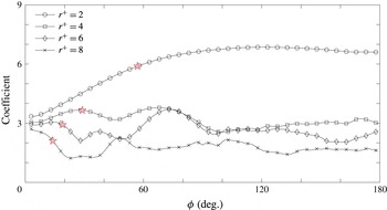
Figure 8 provides further insight into transients decay and the evolution of the flow towards a limit cycle. The sectional pressure force coefficient
 $C_{N}$
(where the sectional, normal, pressure force
 $N$
is computed by integrating the pressure chordwise) obtained in four different spanwise sections located at
 $r^{+}=2$
, 4, 6 and 8 is plotted as a function of
 $\unicode[STIX]{x1D719}$
. A striking feature here is the different trends in
 $C_{N}$
observed for the
 $r^{+}=2$
section on the one hand and for the
 $r^{+}=4$
, 6 and 8 sections on the other hand. First, while the
 $r^{+}=2$
sectional
 $C_{N}$
slowly converges towards a quasi-steady state (reached near
 $\unicode[STIX]{x1D719}=120^{\circ }$
), the
 $C_{N}$
at
 $r^{+}=4$
, 6 and 8 rapidly oscillates around its converged mean value. Second, levels in sectional
 $C_{N}$
at
 $r^{+}=2$
are much higher than those at
 $r^{+}=4$
, 6 and 8. These two very distinct trends reflect differences in the flow structure previously observed between the quasi-steady inboard region and the unsteady outboard region.
Yet, the representation used in figure 8 may introduce bias in the analysis of the flow. Indeed, differences in the evolution of
 $C_{N}$
as a function of
 $\unicode[STIX]{x1D719}$
may partly result from non-uniform local distance of travel along the span. That is, at a given
 $\unicode[STIX]{x1D719}$
, spanwise sections near the wing tip have travelled a longer non-dimensional distance than spanwise sections near the root. Therefore, it is straightforward that spanwise sections near the wing tip converge more rapidly (with respect to
 $\unicode[STIX]{x1D719}$
) towards a limit cycle than spanwise sections near the wing root. To alleviate this potential bias, the non-dimensional local distance of travel (or local convective time)
 $t^{+}=\unicode[STIX]{x1D6FA}r\times t/c=2$
is indicated on each curve by a five-pointed star symbol. It is effectively seen that while these symbols mark a drop in
 $C_{N}$
for the
 $r^{+}=4$
, 6 and 8 sections, the
 $C_{N}$
at
 $r^{+}=2$
still undergoes sustained growth. The drop in
 $C_{N}$
obtained around
 $t^{+}=2$
is consistent with what can be observed on
 $45^{\circ }$
angle of attack translating wings (Taira & Colonius Reference Taira and Colonius2009), which suggest that the flow in the
 $r^{+}=4$
, 6 and 8 sections approaches a nominally two-dimensional flow. That is, the flow physics is driven by similar mechanisms to those found on nominally two-dimensional wings (i.e. vortex shedding and spanwise dislocations due to spanwise instabilities) with three-dimensional mechanisms arising from rotation being weak in comparison. On the contrary, these three-dimensional effects in the
 $r^{+}=2$
section are prominent, which promotes the attachment of the LEV and a globally quasi-steady flow structure.
Sectional pressure coefficient
 $C_{N}$
as a function of the revolution angle
 $\unicode[STIX]{x1D719}$
in 4 spanwise sections located at
 $r^{+}=2$
, 4, 6 and 8. Baseline case:
 $F_{co}=F_{ce}=1$
and
 $Re=500$
. Five-pointed star symbols indicate
 $t^{+}=2$
.

Finally, it can be observed that the trend in
 $r^{+}=8$
sectional
 $C_{N}$
highly resembles that observed for the overall
 $C_{L}$
. Obviously, sectional aerodynamic loads in the most outboard region of the wing have a greater impact on global aerodynamic loads than the most inboard region due to a higher local wing speed. Since global aerodynamic coefficients are obtained by non-dimensionalizing global aerodynamic loads using one global reference speed (
 $\unicode[STIX]{x1D6FA}R/2$
in this paper), as opposed to non-dimensionalizing sectional aerodynamic loads using sectional speeds, they do not reflect the trend in sectional
 $C_{N}$
obtained in the most inboard region (e.g.
 $r^{+}=2$
section) where the local wing speed is weak. In other words, high levels of
 $C_{N}$
obtained in the most inboard region of the wing are somehow hidden by the weak local wing speed. Note that, accordingly, loads obtained at
 $0.75R$
are usually employed as an approximation of global loads on helicopter blades.
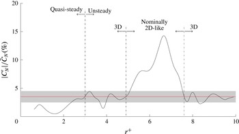
Fluctuating-to-mean sectional pressure coefficients ratio
 $|C_{N}^{\prime }|/\bar{C_{N}}$
as a function of the spanwise location
 $r^{+}$
. Baseline case:
 $F_{co}=F_{ce}=1$
and
 $Re=500$
. The red line indicates the
 $|C_{N}^{\prime }|/\bar{C_{N}}=3.5\,\%$
value and the grey area indicates the
 $\pm 1\,\%$
bounds around this value.
 $C_{N}^{\prime }$
and
 $\bar{C_{N}}$
are computed over the time interval
 $\unicode[STIX]{x1D719}\in [120^{\circ };180^{\circ }]$
.

As initial transients have decayed, fluctuating values of the sectional pressure coefficient can provide additional evidence of the spanwise transition between the quasi-steady inboard region and the unsteady outboard region. Figure 9 shows the distribution in
 $|C_{N}^{\prime }|/\bar{C_{N}}$
(in per cent) along the wing span, where
 $C_{N}^{\prime }$
and
 $\bar{C_{N}}$
are the fluctuating and mean values of
 $C_{N}$
computed over the time interval
 $\unicode[STIX]{x1D719}\in [120^{\circ };180^{\circ }]$
, respectively.
At
 $r^{+}$
values below 2, the
 $|C_{N}^{\prime }|/\bar{C_{N}}$
curve exhibits very weak levels, which is indicative of quasi-steady behaviour. As
 $r^{+}$
increases,
 $|C_{N}^{\prime }|/\bar{C_{N}}$
smoothly increases to reach values of the order of
 $3.5\,\%$
at approximately
 $r^{+}=3$
, indicating the progressive departure from quasi-steady behaviour. Note that the
 $3.5\,\%$
value is displayed in figure 9 using a red horizontal line. Beyond
 $r^{+}=3$
, oscillations in
 $|C_{N}^{\prime }|/\bar{C_{N}}$
around the
 $3.5\,\%$
value highlight spanwise changes in the flow structure. These are followed by a drastic increase in
 $|C_{N}^{\prime }|/\bar{C_{N}}$
at approximately
 $r^{+}=4.9$
. The
 $|C_{N}^{\prime }|/\bar{C_{N}}$
curve then peaks at
 $r^{+}=6.7$
and drops to oscillate again around the
 $3.5\,\%$
value beyond
 $r^{+}=7.6$
.
As such, while the flow can be divided into the quasi-steady inboard region and the unsteady outboard region, with a frontier roughly located around
 $r^{+}=3$
, it is further observed that the outboard region comprises two weakly unsteady three-dimensional subregions at each end, where levels of
 $|C_{N}^{\prime }|/\bar{C_{N}}$
are of the order of
 $3.5\,\%$
. These highlight the influence of relatively strong streamwise vortices (see figure 6) – the TV at the wing tip and the initially shed outboard LEV at the transition between quasi-steady and unsteady regions – which locally damp pressure fluctuations. On the contrary to these three-dimensional weakly unsteady subregions, the nominally two-dimensional-like unsteady subregion between
 $r^{+}=4.9$
and
 $r^{+}=7.6$
exhibits high levels of
 $|C_{N}^{\prime }|/\bar{C_{N}}$
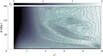
. Figure 10 provides an alternative way of representing these (sub) regions by mapping contours of
 $C_{N}$
as a function of
 $r^{+}$
and
 $\unicode[STIX]{x1D719}$
. Regions of high unsteadiness appear where iso-lines are predominantly in the horizontal direction and, accordingly, where strongest variations in colour contours occur in the vertical direction.
Sectional chordwise pressure coefficient
 $C_{N}$
as a function of the spanwise location
 $r^{+}$
and the revolution angle
 $\unicode[STIX]{x1D719}$
. Baseline case:
 $F_{co}=F_{ce}=1$
and
 $Re=500$
.

4.1.3 Spanwise transition from quasi-steady state to unsteady state
The previous sections put into evidence two distinct regions of the flow: (i) an unsteady outboard region and (ii) a quasi-steady inboard region. For comparison purposes, the frontier between these two regions needs to be rigorously determined. Since there is no consensus on the definition of vortex shedding (and to a larger extent on the definition of a vortex), choosing a criterion that targets the spanwise transition from a stable to an unstable LEV (i.e. from quasi-steady state to unsteady state) is a challenging task. In the previous section,
 $|C_{N}^{\prime }|/\bar{C_{N}}$
levels were found to provide a reasonable estimation of the spanwise location of this transition. However, because an arbitrary threshold on
 $|C_{N}^{\prime }|/\bar{C_{N}}$
levels need to be set to discriminate between quasi-steady and unsteady states, no criterion based on
 $|C_{N}^{\prime }|/\bar{C_{N}}$
levels was found to be sufficiently robust over the whole range of cases tested in this paper.
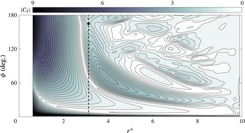
In view of defining a robust criterion for the precise determination of quasi-steady to unsteady states transition, figure 11 maps the absolute sectional chordwise shear coefficient
 $|C_{T}|$
as a function of the sectional non-dimensional blade radius
 $r^{+}$
and the revolution angle
 $\unicode[STIX]{x1D719}$
. It can be seen that the inboard region is characterized by vertical
 $|C_{T}|$
iso-lines which indicate quasi-steady shear forces associated with the attachment of the LEV. Conversely, the outboard region is characterized by strongly inclined
 $|C_{T}|$
iso-lines which indicate shear force fluctuations associated with LEV shedding. Note that a purely two-dimensional (unsteady) flow would lead to strictly horizontal iso-lines. In fact, it can be shown that mapping
 $|C_{T}|$
as a function of
 $t^{+}$
rather than
 $\unicode[STIX]{x1D719}$
leads to horizontal iso-lines in the two-dimensional-like region. Also note that, although it is strongly correlated here, unsteadiness in the LEV imprint on the surface does not necessarily (in the general sense) constitute detachment of the structure. Yet, the representation used in figure 11 suggests that spatial variations in
 $|C_{T}|$
are dominant in the inboard region while temporal variations are dominant in the outboard region. From a topological perspective, this transition between regions dominated by spatial variations on the one hand and temporal variations on the other hand is reflected by saddle points in the
 $|C_{T}|$
map.
Absolute sectional chordwise shear coefficient
 $|C_{T}|$
as a function of the spanwise location
 $r^{+}$
and the revolution angle
 $\unicode[STIX]{x1D719}$
. Baseline case:
 $F_{co}=F_{ce}=1$
and
 $Re=500$
. The black circle indicates the saddle point at the transition between quasi-steady and unsteady regions. The dash-dotted line indicates the corresponding frontier.

On this basis, it is posited that the
 $r^{+}$
value for which the flow evolves from a quasi-steady to an unsteady state (i.e. from a stable to an unstable LEV) is the
 $r^{+}$
value corresponding to the first saddle point encountered as
 $r^{+}$
is increased from the wing root to the wing tip. The search for this saddle point is performed once initial transients have sufficiently decayed, typically for
 $\unicode[STIX]{x1D719}$
values above
 $120^{\circ }$
. This value may however be larger for lower Reynolds number cases, which requires numerical simulations at
 $Re=100$
and 125 to be continued up to
 $\unicode[STIX]{x1D719}=270^{\circ }$
. In addition, the search is performed over
 $r^{+}\in [2;8]$
to avoid any potential bias introduced by root and tip effects.
The dash-dotted line in figure 11 marks the frontier between quasi-steady and unsteady regions obtained using this criterion (the circle indicates the saddle point), which is estimated to be at
 $r_{crit}^{+}=3.1$
for the baseline case. It is seen that the transition between vertical to inclined iso-lines is well captured. This is also found to be the case for the whole range of configurations tested in the following section. In addition, it was verified that, for all cases, the position of this saddle point qualitatively matches the transition as observed from
 $q$
-criterion iso-surfaces. Examples of
 $|C_{T}|$
maps for other configurations are provided in appendix B. It is also interesting to note that a local minimum in
 $|C_{T}|$
is found slightly prior to
 $r_{crit}^{+}$
, i.e. for
 $r^{+}$
of the order of 2.7. However, while this local minimum is a clear indication of the transition from quasi-steady to unsteady regions for the higher Reynolds number cases, it diverges from the actual transition for the lower Reynolds number cases.
4.2 The Coriolis effect
From the above analysis, it appears that the attachment of the LEV is promoted in the inboard region of the wing, leading to a locally quasi-steady flow. Lentink & Dickinson (Reference Lentink and Dickinson2009), Jardin & David (Reference Jardin and David2014, Reference Jardin and David2015) suggested that this attachment and the associated high levels of lift are related to rotational effects, with the Coriolis effect being a key ingredient. In order to provide insight into the influence of the Coriolis effect on the flow topology and on the resulting aerodynamic loads, the Navier–Stokes equations are here manipulated to increase or reduce the relative importance of the Coriolis term with respect to other terms. This is achieved by varying the
 $F_{co}$
factor introduced in § 2.
4.2.1 Influence on the flow structure
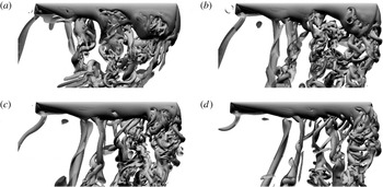
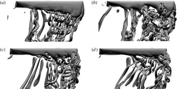
Figure 12 shows iso-surfaces of
 $q$
-criterion obtained at
 $\unicode[STIX]{x1D719}=120^{\circ }$
for
 $F_{co}=0.5$
, 1, 1.5 and 2. As previously,
 $F_{ce}=1$
and
 $Re=500$
. Recall that
 $F_{co}=1$
corresponds to the baseline case.
Iso-surfaces of
 $q$
-criterion (
 $q^{+}=0.25$
and 2.5) obtained at revolution angle
 $\unicode[STIX]{x1D719}=120^{\circ }$
. Cases
 $F_{co}=0.5$
(a), 1 (b), 1.5 (c) and 2 (d) at
 $Re=500$
and with
 $F_{ce}=1$
.

The overall comparison seems to indicate that LEV attachment is maintained at higher
 $r^{+}$
values as
 $F_{co}$
is increased and vice versa. While small-scale structures nearly cover the entire wing span in the
 $F_{co}=0.5$
case, they hardly extend over the midspan in the
 $F_{co}=2$
case. These small-scale structures indicate unsteadiness in the outboard region of the wing, as opposed to a stably attached LEV in the inboard region. For the sake of comparison, the reader can refer to the position of the initially shed outboard LEV that was previously found to approximate the location of the transition from the quasi-steady region to the unsteady region. Therefore, there is clear evidence that the Coriolis effect is a key element in LEV stability observed in the inboard region of revolving wings.
Contours of non-dimensional vorticity magnitude
 $\unicode[STIX]{x1D714}^{+}$
obtained in a spanwise cross-section located 2 chords away from the axis of rotation at 6 revolution angles (from top to bottom). Cases
 $F_{co}=0.5$
, 1, 1.5 and 2 (from a to d) at
 $Re=500$
and with
 $F_{ce}=1$
.

Contours of non-dimensional spanwise velocity
 $v_{z}^{+}$
obtained in a spanwise cross-section located 2 chords away from the axis of rotation at 3 revolution angles (from top to bottom). Cases
 $F_{co}=0.5$
, 1, 1.5 and 2 (from a to d) at
 $Re=500$
and with
 $F_{ce}=1$
.

Contours of non-dimensional spanwise pressure gradients
 $\unicode[STIX]{x2202}p^{+}/\unicode[STIX]{x2202}z$
obtained in a spanwise cross-section located 2 chords away from the axis of rotation at 3 revolution angles (from top to bottom). Cases
 $F_{co}=0.5$
, 1, 1.5 and 2 (from a to d) at
 $Re=500$
and with
 $F_{ce}=1$
.

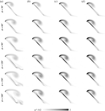
Figure 13 shows corresponding iso-contours of vorticity magnitude obtained in a spanwise cross-section located 2 chords away from the axis of rotation (i.e. quasi-steady region), at revolution angles
 $\unicode[STIX]{x1D719}=30^{\circ }$
,
 $60^{\circ }$
,
 $90^{\circ }$
,
 $120^{\circ }$
and
 $180^{\circ }$
. It can be seen that increasing
 $F_{co}$
leads to a more compact LEV that remains closer to the wing surface. This more compact pattern is associated with slightly higher vorticity levels. In particular, the most striking differences appear through a stronger shear layer emanating from the leading edge, an increased vorticity magnitude in the core of the LEV and, consequently, a stronger boundary layer on the wing upper surface with increasing
 $F_{co}$
. In addition, it appears that the LEV reaches a quasi-steady state more rapidly as
 $F_{co}$
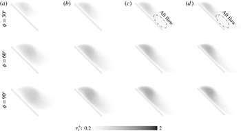
increases. Because strong spanwise velocities mostly develop in the core of the LEV, the distribution of spanwise velocity displayed in figure 14 also exhibits a more compact pattern as
 $F_{co}$
is increased. Note that figure 14 only displays contours for
 $\unicode[STIX]{x1D719}\leqslant 90^{^{\circ }}$
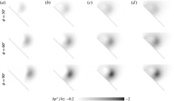
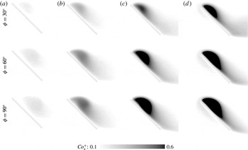
, which correspond to the growth phase of the LEV. Spanwise flow in the core of the LEV is principally driven by spanwise gradients in flow speed (Jardin & David Reference Jardin and David2014) and resulting spanwise pressure gradients. Evidence of strong spanwise pressure gradients in the core of the LEV are provided in figure 15. However, it appears that the Coriolis effect also plays a non-negligible role in levels of spanwise pressure gradients, hence in the development of the core flow. It can be seen from figure 15 that levels of
 $\unicode[STIX]{x2202}p^{+}/\unicode[STIX]{x2202}z$
increase with
 $F_{co}$
and that this effect appears early in the motion (e.g. see
 $\unicode[STIX]{x1D719}=30^{\circ }$
). Thus, the Coriolis effect contributes to outboard vorticity transport in the core of the LEV, hence limiting LEV growth early in the motion and promoting LEV stability. This augments previous observations by Jardin & David (Reference Jardin and David2014) who showed that rotational effects (Coriolis and centrifugal) increase spanwise velocity in the core of the LEV in comparison to that observe in the sole presence of spanwise gradients in flow speed (i.e. without Coriolis and centrifugal effects). Furthermore, another striking feature is the development of a region of spanwise flow immediately downstream the LEV, close to the wing surface, with increasing
 $F_{co}$
. This region, indicated by an ellipse in figure 14, has also been observed in previous works (Birch & Dickinson Reference Birch and Dickinson2001; Birch, Dickson & Dickinson Reference Birch, Dickson and Dickinson2004; Poelma, Dickson & Dickinson Reference Poelma, Dickson and Dickinson2006; Aono, Liang & Liu Reference Aono, Liang and Liu2008). Interestingly, Lentink & Dickinson (Reference Lentink and Dickinson2009) hypothesized that the Coriolis effect is a necessary condition for this spanwise flow to develop, based on theoretical considerations. It is here shown that the Coriolis effect does promote spanwise flow behind the LEV (visible early in the motion), which may contribute to both outboard vorticity drainage and increased momentum in the aft boundary layer. It is believed that outboard vorticity drainage helps balance the production of vorticity at the leading edge (Ellington et al.
Reference Ellington, Van den Berg, Willmott and Thomas1996) and increased momentum behind the LEV helps stabilize the aft boundary layer, thereby promoting the attachment of the LEV.
Contours of non-dimensional spanwise Coriolis acceleration
 $Co_{z}^{+}$
obtained in a spanwise cross-section located 2 chords away from the axis of rotation at 3 revolution angles (from top to bottom). Cases
 $F_{co}=0.5$
, 1, 1.5 and 2 (from a to d) at
 $Re=500$
and with
 $F_{ce}=1$
.

Contours of non-dimensional streamwise Coriolis acceleration
 $Co_{x}^{+}$
obtained in a spanwise cross-section located 2 chords away from the axis of rotation at 3 revolution angles (from top to bottom). Cases
 $F_{co}=0.5$
, 1, 1.5 and 2 (from a to d) at
 $Re=500$
and with
 $F_{ce}=1$
.

The correlation between the Coriolis effect and outboard flow can be explained as follows. Consider still air. In a non-inertial frame of reference with rotation speed
 $\unicode[STIX]{x1D6FA}$
, the flow velocity can simply be expressed as
 $u=-\unicode[STIX]{x1D6FA}\times r$
, where
 $r$
is the radial distance from the rotation axis. Centrifugal and Coriolis accelerations apply in this non-inertial reference frame. The Coriolis acceleration
 $-2\unicode[STIX]{x1D6FA}\times u$
is oriented radially, towards the rotation axis. Although a fluid particle experiences this radial acceleration, it has no radial velocity. Now if a wing that rotates with the non-inertial, rotating frame is introduced (i.e. its speed in the non-inertial frame of reference is zero), then
 $u$
will be modified, which in turn modifies the Coriolis acceleration. Specifically, in recirculation regions where the magnitude of
 $u$
is reduced (or where
 $u$
changes sign), the magnitude of the Coriolis acceleration is reduced (or the Coriolis acceleration changes sign). Hence, when compared with the ‘still air’ case where there is no radial velocity, fluid particles in regions of reduced
 $u$
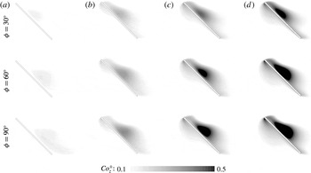
(induced by the wing) will tend to move outboard. As such, reduced velocity in the LEV promotes outboard flow through the Coriolis term. Figure 16 shows iso-contours of the spanwise Coriolis acceleration in a spanwise cross-section located 2 chords away from the axis of rotation, at revolution angles
 $\unicode[STIX]{x1D719}=30^{\circ }$
,
 $60^{\circ }$
and
 $90^{\circ }$
. To clearly reveal the Coriolis effect induced by the presence of the wing, the Coriolis acceleration that applies in the ‘still air’ case is subtracted: i.e.
 $Co_{z}=-2\unicode[STIX]{x1D6FA}F_{co}\times (u+\unicode[STIX]{x1D6FA}\times r)$
is displayed. It can be seen that regions where the magnitude of the streamwise flow velocity in the non-inertial frame of reference is reduced (or where the streamwise velocity changes sign) – in the core, below and behind the LEV – are associated with an increase in Coriolis acceleration that can be correlated with the extent of outboard velocity and pressure gradients in figures 14 and 15. The enhancement of outboard velocity in turn increases the streamwise component of the Coriolis acceleration (figure 17), oriented towards the trailing edge (i.e. opposed to the adverse pressure gradient). Interestingly, because the centrifugal term only depends on operating parameters (
 $\unicode[STIX]{x1D6FA}$
and
 $r$
), and not on the local flow velocity
 $u$
, it will not be directly modified by introducing the wing. Thus, although changes in the whole flow field may indirectly tend to modify the centrifugal term through a global equilibrium of all terms in the Navier–Stokes equations, the present interpretation suggests that changes in
 $F_{ce}$
may have a negligible impact on the stability of the LEV. This will be further addressed in § 4.2.3.
Finally, the balance between the Coriolis term and the other terms in the Navier–Stokes equations (i.e. which is modified through
 $F_{co}$
) is also reflected in the trajectory of shed vortices. While shed vortices in the wake of the
 $F_{co}=1$
baseline case roughly follow circular trajectories about the rotation axis, they tend to move inboard and outboard in the
 $F_{co}<1$
and
 $F_{co}>1$
cases respectively (figure 12).
4.2.2 Influence on global and sectional forces
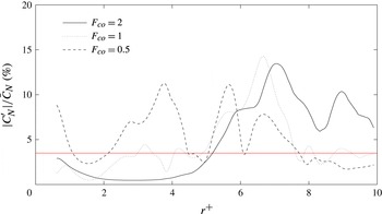
Figure 18 shows the distribution in
 $|C_{N}^{\prime }|/\bar{C_{N}}$
(in per cent) along the wing span obtained for the
 $F_{co}=0.5$
(dashed line) and
 $F_{co}=2$
(plain line) cases. The
 $F_{co}=1$
case previously shown in figure 9 is added for the sake of comparison.
Fluctuating-to-mean pressure coefficients ratio
 $|C_{N}^{\prime }|/\bar{C_{N}}$
as a function of the spanwise location
 $r^{+}$
. Cases
 $F_{co}=0.5$
and 2 at
 $Re=500$
and with
 $F_{ce}=1$
. The red line indicates the
 $|C_{N}^{\prime }|/\bar{C_{N}}=3.5\,\%$
value.
 $C_{N}^{\prime }$
and
 $\bar{C_{N}}$
are computed over the time interval
 $\unicode[STIX]{x1D719}\in [120^{\circ };180^{\circ }]$
.

First, it is shown that the sharp increase in
 $|C_{N}^{\prime }|/\bar{C_{N}}$
levels as
 $r^{+}$
increases occurs near
 $r^{+}=2$
for
 $F_{co}=0.5$
and near
 $r^{+}=5$
for
 $F_{co}=2$
. This is in line with previous observations on flow topology. The severe impact of an increased Coriolis effect on LEV attachment is further highlighted by an almost complete damping of
 $|C_{N}^{\prime }|/\bar{C_{N}}$
levels between approximately
 $r^{+}=2$
and
 $r^{+}=4$
in the
 $F_{co}=2$
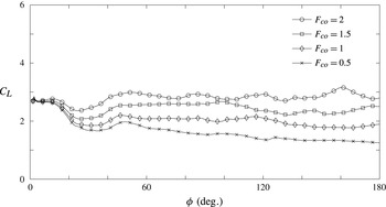
case. A consequence of enhanced LEV stability for higher
 $F_{co}$
values is an increase in global lift coefficient (figure 19).
Second, it is observed that the influence of the TV on
 $|C_{N}^{\prime }|/\bar{C_{N}}$
is also modified as
 $F_{co}$
varies. For the
 $F_{co}=0.5$
case, the lower relative strength of the Coriolis acceleration with respect to other terms pulls the TV inboard, thereby increasing its influence on
 $|C_{N}^{\prime }|/\bar{C_{N}}$
levels. The latter’s are found to be damped near the wing tip, when compared to those observed in the
 $F_{co}=1$
baseline case. On the contrary, the stronger relative strength of the Coriolis acceleration with respect to other terms in the
 $F_{co}=2$
case tends to push the TV outboard. Hence,
 $|C_{N}^{\prime }|/\bar{C_{N}}$
exhibits relatively strong levels up to
 $r^{+}=10$
.
Finally, one can notice that decreasing
 $F_{co}$
also results in relatively strong levels of
 $|C_{N}^{\prime }|/\bar{C_{N}}$
at the wing root. The underlying unsteadiness is not related to any LEV instability, but to changes in the trajectory of the sTEV which, as a consequence, interacts with the wing in the vicinity of the root.
Changes in flow unsteadiness due to intrinsic LEV instability should be carefully isolated from those due to modifications in TV and sTEV trajectories. It is thus noteworthy to emphasize that, in order to avoid any misinterpretation, the search for
 $r_{crit}^{+}$
using the saddle point criterion is performed over
 $r^{+}\in [2;8]$
. That is, root and tip regions where the TV and the sTEV may affect the LEV are excluded.
Lift coefficient
 $C_{L}$
as a function of the revolution angle
 $\unicode[STIX]{x1D719}$
. Cases
 $F_{co}=0.5$
, 1, 1.5 and 2 at
 $Re=500$
and with
 $F_{ce}=1$
.

4.2.3 Influence on the spanwise transition and interplay with centrifugal and viscous effects
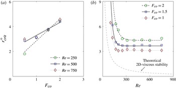
The
 $r_{crit}^{+}$
value for which the flow evolves from a quasi-steady state to an unsteady state is plotted as a function of
 $F_{co}$
on figure 20(a). The results are shown for
 $Re=500$
as well as for
 $Re=250$
and
 $Re=750$
. This overall picture shows the dependency of LEV attachment on the Coriolis effect. Recall that in all cases addressed in this paper,
 $F_{ce}$
is set to 1. However, in order to evaluate the importance of the interplay between Coriolis and centrifugal effects cases at
 $Re=500$
, where
 $F_{ce}=F_{co}$
, are added.
As previously discussed, figure 20(a) shows that
 $r_{crit}^{+}$
increases with increasing
 $F_{co}$
. It further suggests that the relation between
 $r_{crit}^{+}$
and
 $F_{co}$
is roughly linear within the range of
 $F_{co}$
tested. Linear trend lines are depicted to illustrate this relation. Moreover, it can be seen that the slope of the linear trend lines is dependent on the Reynolds number. This suggests that the Coriolis effect may not act in a similar way at high and low Reynolds numbers.
On the contrary, it is demonstrated that centrifugal effects have a negligible impact on LEV stability as
 $r_{crit}^{+}$
is unchanged whether
 $F_{ce}$
is set to 1 or equal to
 $F_{co}$
. For the sake of completeness, iso-surfaces of
 $q$
-criterion and contours of vorticity and spanwise velocity obtained for different values of
 $F_{ce}$
at
 $F_{co}=2$
are displayed in figures 21 and 22 respectively. Values of 0, 1, 2 and 4 are considered for
 $F_{ce}$
, which correspond to cases where centrifugal effects are suppressed, unchanged, changed linearly and quadratically with respect to the Coriolis effect respectively. The last case, where
 $F_{ce}=4$
, is consistent with the fact that the Coriolis term in the Navier–Stokes equation is an explicit linear function of the rotation speed whereas the centrifugal term is an explicit quadratic function. Here again, it is shown that
 $F_{ce}$
has a negligible impact on the flow structure. In particular, compactness of the LEV and spanwise flow behind the LEV coexists for all values of
 $F_{ce}$
. This augments previous findings by Jardin & David (Reference Jardin and David2015) and supports the idea that the influence of the Coriolis factor
 $F_{co}$
can be investigated at fixed
 $F_{ce}$
. It should be noted that this differs from previous results by Garmann & Visbal (Reference Garmann and Visbal2014) who concluded on the apparent dominant role of centripetal acceleration on LEV stability at slightly higher Reynolds numbers (
 $Re>1000$
).
Position of the transition from quasi-steady state to unsteady state
 $r_{crit}^{+}$
as a function of the Coriolis factor
 $F_{co}$
for
 $Re=250$
, 500 and 750 (a) and as a function of the Reynolds number
 $Re$
for
 $F_{co}=1$
, 1.5 and 2 (b) with
 $F_{ce}=1$
. Cases at
 $Re=500$
and with
 $F_{ce}=F_{co}$
are added in (a) and indicated using a
 $+$
symbol.
 $Re\in [100;750]$
are considered in (b).

Iso-surfaces of
 $q$
-criterion (
 $q^{+}=0.25$
and 2.5) obtained at revolution angle
 $\unicode[STIX]{x1D719}=120^{\circ }$
. Cases
 $F_{ce}=0$
(a), 1 (b), 2 (c) and 4 (d) at
 $Re=500$
and with
 $F_{co}=2$
.

To gain further insight into the interplay between the Coriolis effect and viscous effects,
 $r_{crit}^{+}$
is plotted as a function of
 $Re$
on figure 20(b). The results are shown for
 $F_{co}=1$
, 1.5 and 2. Overall, two distinct trends are observed whether the Reynolds number is in the higher or in the lower range of
 $Re$
values tested.
In the higher range
 $Re\in [200;750]$
, all
 $F_{co}$
curves are roughly horizontal, demonstrating that
 $r_{crit}^{+}$
is weakly dependent on
 $Re$
. In contrast, and as previously put into evidence, vertical offsets between distinct
 $F_{co}$
curves indicate that
 $r_{crit}^{+}$
is more critically dependent on
 $F_{co}$
. In other words,
 $r_{crit}^{+}$
clearly appears to be more sensitive to changes in
 $F_{co}$
than it is to changes in
 $Re$
, for
 $Re>200$
. That is, the Coriolis effect has the dominant role in vortex stability. While this is true for
 $Re\in [200;750]$
, additional cases should be investigated to verify whether or not this holds for higher Reynolds numbers. This cannot be achieved here due to computational costs. Nonetheless, it can be mentioned that the asymptotic value obtained for
 $F_{co}=1$
as
 $Re$
increases is consistent with observations reported by Kruyt et al. (Reference Kruyt, van Heijst, Altshuler and Lentink2015) at Reynolds numbers
 $O(10^{4})$
.
In the lower range,
 $Re<200$
,
 $r_{crit}^{+}$
is highly dependent on
 $Re$
. It is shown that all
 $F_{co}$
curves exponentially increase with decreasing
 $Re$
. Here,
 $r_{crit}^{+}$
is more sensitive to changes in
 $Re$
than it is to changes in
 $F_{co}$
such that viscous effects appear to be the key factor in LEV stability. Overall, it is believed that viscous effects affect the behaviour of the LEV in a qualitatively similar way than they would affect a LEV on a two-dimensional wing. At these low Reynolds numbers, viscous effects become determinant in LEV stability on a two-dimensional wing. In particular, for
 $\unicode[STIX]{x1D6FC}=45^{\circ }$
, it is known that the flow is stable for
 $Re$
values below 50 (Zhang, Liu & Lu Reference Zhang, Liu and Lu2009; Choi, Colonius & Williams Reference Choi, Colonius and Williams2015). If the flow around a rotating wing is considered as quasi-two-dimensional, in the sense that the flow at each spanwise section of the wing is considered as a two-dimensional one, then the LEV in a specific spanwise section should be stabilized by viscous effects if the local Reynolds number
 $re=\unicode[STIX]{x1D714}rc/\unicode[STIX]{x1D708}$
is below 50. The local Reynolds number
 $re$
can simply be expressed as a function of the global Reynolds number
 $Re=\unicode[STIX]{x1D714}(R/2)c/\unicode[STIX]{x1D708}$
, such that
 $re=Re/(R/2)\times r$
. Therefore, under the assumption of quasi-two-dimensionality, the flow is locally stabilized (in a spanwise section) if
 $re<50\Rightarrow r<(50/Re)\times (R/2)$
. The theoretical value
 $r_{crit,2D}^{+}=(50/Re)\times (R/2)$
is depicted as a grey dash-dotted line in figure 20(b). It can be seen that the trend in
 $r_{crit}^{+}$
obtained from the present numerical simulations as
 $Re$
decreases below 200 is qualitatively similar to that obtained from two-dimensional considerations. This supports the idea that viscous effects are the key element in LEV stability for
 $Re$
below 200.
Contours of non-dimensional vorticity magnitude
 $\unicode[STIX]{x1D714}^{+}$
and spanwise velocity
 $v_{z}^{+}$
obtained in a spanwise cross-section located 2 chords away from the axis of rotation at revolution angle
 $\unicode[STIX]{x1D719}=120^{\circ }$
. Cases
 $F_{ce}=0$
, 1, 2 and 4 (from a to d) at
 $Re=500$
and with
 $F_{co}=2$
.

A key hypothesis in LEV stability is that spanwise flow balances vorticity production at the leading edge, preventing indefinite growth of the LEV (Ellington et al.
Reference Ellington, Van den Berg, Willmott and Thomas1996; Lentink & Dickinson Reference Lentink and Dickinson2009). Spanwise flow in the core of the LEV is principally driven by spanwise pressure gradients resulting from spanwise gradients in flow speed (Jardin & David Reference Jardin and David2014). It is shown here that the Coriolis effect also contributes to increasing spanwise flow by enhancing pressure gradients. This not only results in higher levels of spanwise velocity in the core of the LEV but also in the development of a region of spanwise flow behind the LEV, close to the wing surface. Spanwise flow behind the LEV most certainly contributes to outboard vorticity transport but may also stabilize the aft boundary layer. While spanwise flow behind the LEV is generally observed for a range of Reynolds numbers
 $O(10^{2}-10^{3})$
, spanwise flow in the core of the LEV seems to be inhibited at lower Reynolds numbers
 $O(10^{2})$
(Birch et al.
Reference Birch, Dickson and Dickinson2004; Poelma et al.
Reference Poelma, Dickson and Dickinson2006; Aono et al.
Reference Aono, Liang and Liu2008) because viscous effects tend to ‘homogenize’ the flow and to mitigate velocity gradients. This suggests that mechanisms of vorticity transport are reduced at lower Reynolds numbers. However, in light of the results presented in this paper, it is believed that the reduction in spanwise velocity as
 $Re$
decreases is not a critical issue to LEV stability precisely because viscous effects become predominant in LEV stability in the lower
 $Re$
range.
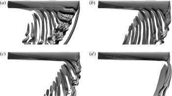
Iso-surfaces of
 $q$
-criterion (
 $q^{+}=0.25$
and 2.5) obtained for angle of attack
 $\unicode[STIX]{x1D6FC}=15^{\circ }$
at revolution angle
 $\unicode[STIX]{x1D719}=120^{\circ }$
. Cases
 $F_{co}=0.5$
(a), 1 (b), 1.5 (c) and 2 (d) at
 $Re=500$
and with
 $F_{ce}=1$
.

Iso-surfaces of
 $q$
-criterion (
 $q^{+}=0.25$
and 2.5) obtained for angle of attack
 $\unicode[STIX]{x1D6FC}=30^{\circ }$
at revolution angle
 $\unicode[STIX]{x1D719}=120^{\circ }$
. Cases
 $F_{co}=0.5$
(a), 1 (b), 1.5 (c) and 2 (d) at
 $Re=500$
and with
 $F_{ce}=1$
.

4.2.4 Generalization to other post-stall angles of attack
The influence of the Coriolis acceleration on the LEV is analysed for two additional post-stall angles of attack,
 $\unicode[STIX]{x1D6FC}=15^{\circ }$
and
 $\unicode[STIX]{x1D6FC}=30^{\circ }$
. Figures 23 and 24 show the corresponding iso-surfaces of
 $q$
-criterion obtained at
 $\unicode[STIX]{x1D719}=120^{\circ }$
for
 $F_{co}=0.5$
, 1, 1.5 and 2. Again,
 $F_{ce}$
is set to 1 and
 $Re=500$
. Similarly to the
 $\unicode[STIX]{x1D6FC}=45^{\circ }$
case, it is observed that increasing
 $F_{co}$
promotes LEV attachment. However, it appears that
 $F_{co}$
has a greater authority as
 $\unicode[STIX]{x1D6FC}$
decreases. This is particularly striking for
 $\unicode[STIX]{x1D6FC}=15^{\circ }$
where increasing
 $F_{co}$
to 2 completely suppresses outboard unsteadiness. This increased authority at lower
 $\unicode[STIX]{x1D6FC}$
can be related to a weaker LEV that is more easily ‘controllable’. Because the Coriolis effect has a stronger authority at lower
 $\unicode[STIX]{x1D6FC}$
, the position of the spanwise transition from a stable to an unstable LEV moves outboard with decreasing
 $\unicode[STIX]{x1D6FC}$
, when holding
 $F_{co}$
constant. This is observed by comparing figures 12, 23 and 24. The fact that a weaker LEV (with lower growth rate) is more easily ‘controllable’ is consistent with the hypothesis that outboard vorticity transport balances vorticity production at the leading edge. It is also consistent with the hypothesis that spanwise flow behind the LEV stabilizes the aft boundary layer, which is less prone to separation as
 $\unicode[STIX]{x1D6FC}$
decreases. On the other hand, it is known that flows at low angles of attack are more easily ‘controllable’ than flows at high angles of attack. Interestingly, these results open the path towards potential flow control strategies that mimic the Coriolis effect to delay stall and enhance lift on translating wings. In addition, these indicate that low-order models of rotating wing aerodynamics, such as blade element models, should account for the Coriolis effect and its dependence on the angle of attack.
5 Conclusion
If the angle of attack and Reynolds number are sufficiently high, the flow past a two-dimensional translating wing is unstable. Conversely, at similar angle of attack and Reynolds number, the flow past a revolving wing may locally (in a given spanwise section) be stable. This stability is usually associated with the presence of a LEV that remains robustly attached to the wing. LEV attachment on revolving (or rotating) wings is a ubiquitous feature observed in nature and it is now widely admitted as being responsible for the unexpected high lift observed on insect flapping wings and autorotating plant seeds, for example. Recent studies suggest that the attachment of the LEV on revolving wings originates in rotational accelerations, with the Coriolis effect being a key element. As such, it is usually observed in a region extending from the axis of rotation to 3 or 4 chords away from it (i.e. where rotational effects are strong).
In this paper, the behaviour of the LEV that develops on a high angle of attack, aspect ratio 9.5, revolving wing and its dependency on the Coriolis effect are analysed. Toward that end, the Navier–Stokes equations are solved in the non-inertial reference frame of the wing with the Coriolis term being artificially tuned. Reynolds numbers in the range
 $Re\in [100;750]$
are considered to identify the interplay between Coriolis and viscous effects. Similarly, artificial tuning of the centrifugal term is achieved to identify the interplay between Coriolis and centrifugal effects.
First, it is shown that flow stability and robust LEV attachment are promoted in the inboard region of the wing, where rotational accelerations are strong. Conversely, the flow in the outboard region of the wing is unstable and exhibits a nominally two-dimensional-like, highly unsteady region bounded by two weakly unsteady three-dimensional regions. Three-dimensional regions are dominated by strong streamwise vortices that arise from the free tip condition on the one hand and from the transition between stable and unstable flow regions on the other hand. The transition between inboard quasi-steady and outboard unsteady flow regions is found to be reasonably approximated by saddle points in the spatio-temporal map of sectional shear force on the wing. Saddle points can be viewed as a transition between regions dominated by spatial variations in sectional shear force and those dominated by temporal variations.
The saddle point criterion is used to quantify the correlation between the Coriolis effect and the position of the transition along the span for Reynolds numbers in the range
 $Re\in [100;750]$
. It is shown that the transition between quasi-steady and unsteady regions is pushed towards the wing tip as the Coriolis term in the Navier–Stokes equations is artificially increased. This provides further evidence that the Coriolis effect has an important role in flow stability on revolving wings.
The present results reveal that Coriolis effect promotes spanwise pressure gradients and resulting spanwise flow. A particular feature is that the Coriolis effect is not only correlated with an increased velocity inside the core of the LEV (where pressure gradients due to spanwise gradients in flow speed are strong), but also with the development of a region of spanwise flow behind the LEV. Interestingly, this aft flow has been observed in the past and theoretical considerations suggested that it could be related to the Coriolis effect (Lentink & Dickinson Reference Lentink and Dickinson2009). While the overall enhancement of spanwise flow is believed to contribute to outboard vorticity transport, spanwise flow behind the LEV may also tend to stabilize the aft boundary layer.
Furthermore, it is shown that the Coriolis effect dominates flow stability for Reynolds numbers above 200 where the transition appears to be weakly dependent on
 $Re$
, and since centrifugal effects are found to have no significant impact on the flow field. In contrast, the analysis demonstrates that the role of viscous effects become prominent as
 $Re$
decreases below 200. In particular, for
 $Re<200$
, the trend in the position of the transition point as a function of
 $Re$
resembles that deduced from two-dimensional cases where stability only relies on viscous effects (i.e. not on rotational effects). It is therefore suggested that the reduction in spanwise velocity in the core of the vortex as
 $Re$
decreases (which has been observed in previous works and reduces the potential for outboard vorticity transport) is not a critical issue to LEV stability because viscous effects become predominant in LEV stability in the lower
 $Re$
range.
Finally, while the analysis is principally conducted for wings with angle of attack
 $\unicode[STIX]{x1D6FC}=45^{\circ }$
, additional cases with
 $\unicode[STIX]{x1D6FC}=15^{\circ }$
and
 $\unicode[STIX]{x1D6FC}=30^{\circ }$
show that the Coriolis effect has greater authority on the attachment of the LEV as
 $\unicode[STIX]{x1D6FC}$
decreases.
Overall, this work provides insight into the mechanisms that contribute to flow stability and LEV attachment on revolving wings. Besides, it opens the path towards the development of enhanced low-order models (e.g. blade element models) accounting for rotational effects as well as the definition of control strategies mimicking rotational effects for stall delay on translating wings. The conclusions drawn here are valid for low Reynolds numbers
 $O(10^{2}-10^{3})$
and additional cases should be considered in the future to evaluate to what extent these conclusions hold at higher Reynolds numbers.
Appendix A. Temporal resolution
Figure 25 compares the instantaneous lift and torque coefficients obtained using the reported temporal resolution
 $\unicode[STIX]{x0394}t=2\unicode[STIX]{x03C0}/720$
with those obtained by decreasing the time step by a factor of 2 (
 $\unicode[STIX]{x0394}t=2\unicode[STIX]{x03C0}/1440$
), 4 (
 $\unicode[STIX]{x0394}t=2\unicode[STIX]{x03C0}/2880$
) and 8 (
 $\unicode[STIX]{x0394}t=2\unicode[STIX]{x03C0}/5760$
). Here again, slight discrepancies exist for revolution angles larger than
 $\unicode[STIX]{x1D719}=90^{\circ }$
, i.e. when initial transients have decayed and a large portion of the wing, outboard, exhibits unsteady flow structures. In all cases, the curves lie within
 $\pm 6\,\%$
bounds around the values obtained using the finest temporal resolution
 $\unicode[STIX]{x0394}t=2\unicode[STIX]{x03C0}/5760$
(indicated by the grey area). Overall, the main effect of
 $\unicode[STIX]{x0394}t$
is to phase shift fluctuations of lift and torque, for later
 $\unicode[STIX]{x1D719}$
values. Because the flow outboard is chaotic, it is expected that slight modifications in the numerical set-up would lead to slight changes in the timing of shedding of small-scale structures. That is, oscillations due to small scale structures are phase shifted but their amplitudes do not change. As a result, it can be shown that the mean lift and torque coefficients are almost unchanged as
 $\unicode[STIX]{x0394}t$
is varied. Mean values obtained in the range of
 $\unicode[STIX]{x0394}t$
considered here match within 1 %.
Coefficients of lift
 $C_{L}$
and torque
 $C_{Q}$
as a function of the revolution angle
 $\unicode[STIX]{x1D719}$
for different temporal resolutions
 $\unicode[STIX]{x0394}t$
.

Absolute sectional chordwise shear coefficient
 $|C_{T}|$
as a function of the spanwise location
 $r^{+}$
and the revolution angle
 $\unicode[STIX]{x1D719}$
. Cases
 $Re=250$
and
 $F_{co}=1$
(a),
 $Re=750$
and
 $F_{co}=2$
(b) and
 $Re=100$
and
 $F_{co}=2$
(c).

Appendix B. Sectional chordwise shear coefficient
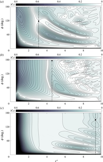
Figure 26 displays three additional examples of
 $|C_{T}|$
maps. Contours and iso-lines of
 $|C_{T}|$
are depicted as a function of the spanwise location
 $r^{+}$
and the revolution angle
 $\unicode[STIX]{x1D719}$
for cases
 $Re=250$
,
 $F_{co}=1$
(a),
 $Re=750$
,
 $F_{co}=2$
(b) and
 $Re=100$
,
 $F_{co}=2$
(c). In all cases, iso-lines are displayed by steps of 0.02 in the range
 $|C_{T}|\in [0;0.8]$
. The first case (
 $Re=250$
,
 $F_{co}=1$
) is a typical example showing how interactions between the wing and the root vortex may introduce bias in the search for the transition from a stable to an unstable LEV. Distortion of vertical iso-lines are observed for
 $r^{+}<2$
. The second case (
 $Re=750$
,
 $F_{co}=2$
) is very similar to the baseline case addressed in detail in the paper, yet with a transition point pushed towards the wing tip. The third case (
 $Re=100$
,
 $F_{co}=2$
) is a typical case showing quasi-steady state over the whole wing span. Very few iso-lines appear for
 $r^{+}>2$
, which indicates no significant spatial and temporal variations in
 $|C_{T}|$
. The saddle point identified near the wing tip is here due to the influence of the tip vortex and is not indicative of any intrinsic LEV instability. That is, the saddle point would be found at higher
 $r^{+}$
value if a higher aspect ratio wing was used. One can also note that the quasi-steady state is reached for relatively large
 $\unicode[STIX]{x1D719}$
values (i.e. above 120
 $^{\circ }$
).