2 Görtler vortices – basic scalings and governing equations

We consider an incompressible boundary layer flow over a concave surface, with upstream perturbations provided by a spanwise periodic array of roughness elements at some downstream streamwise location, $x^{\ast }=x_{0}^{\ast }$ (hereafter all dimensional quantities have a star). The boundary layer flow configuration is the same as that considered in Sescu & Thompson (Reference Sescu and Thompson2015) or Sescu et al. (Reference Sescu, Taoudi and Afsar2017) (see figure 1 in Sescu & Thompson Reference Sescu and Thompson2015). The effect of the roughness elements is not directly modelled here, but taken into account as initial condition from an asymptotic solution derived previously in Goldstein et al. (Reference Goldstein, Sescu, Duck and Choudhari2010). The spanwise length scale of the roughness row, $\unicode[STIX]{x1D6EC}^{\ast }$ , is of the same order of magnitude as the local boundary layer thickness $\unicode[STIX]{x1D6FF}^{\ast }\equiv x_{0}^{\ast }/\sqrt{R}=x_{0}^{\ast }\unicode[STIX]{x1D6FF}$ at the roughness location $x_{0}^{\ast }$ , where $R=x_{0}^{\ast }U_{\infty }^{\ast }/\unicode[STIX]{x1D708}^{\ast }$ is the Reynolds number based on $x_{0}^{\ast }$ and $U_{\infty }^{\ast }$ is the free-stream velocity, with $\unicode[STIX]{x1D708}^{\ast }$ being the kinematic viscosity, and $\unicode[STIX]{x1D6FF}\equiv R^{-1/2}$ being the boundary layer thickness scaled by the (fixed) $O(1)$ length scale, $\unicode[STIX]{x1D6EC}^{\ast }$ . The spatial coordinates are normalized by the spanwise length scale, $\unicode[STIX]{x1D6EC}^{\ast }$ , as $(x,y,z)=(x^{\ast },y^{\ast },z^{\ast })/\unicode[STIX]{x1D6EC}^{\ast }$ , and the velocity and pressure are normalized as

(2.1a-d ) $$\begin{eqnarray}\displaystyle \tilde{u} =\frac{u^{\ast }}{U_{\infty }^{\ast }},\quad \tilde{v}=R_{\unicode[STIX]{x1D6EC}}\frac{v^{\ast }}{U_{\infty }^{\ast }},\quad \tilde{w}=R_{\unicode[STIX]{x1D6EC}}\frac{w^{\ast }}{U_{\infty }^{\ast }},\quad \tilde{p}=R_{\unicode[STIX]{x1D6EC}}^{2}\frac{p^{\ast }}{\unicode[STIX]{x1D70C}^{\ast }U_{\infty }^{\ast 2}}, & & \displaystyle\end{eqnarray}$$

where $(u^{\ast },v^{\ast },w^{\ast })$ is the dimensional velocity vector, $\unicode[STIX]{x1D70C}^{\ast }$ is the density and $R_{\unicode[STIX]{x1D6EC}}=U_{\infty }^{\ast }\unicode[STIX]{x1D6EC}^{\ast }/\unicode[STIX]{x1D708}^{\ast }$ is the Reynolds number based on $\unicode[STIX]{x1D6EC}^{\ast }$ . Görtler vortices are expected to develop when $x\sim 2\unicode[STIX]{x03C0}/k_{1}\sim \unicode[STIX]{x1D6EC}^{\ast }R_{\unicode[STIX]{x1D6EC}}$ (Wu, Zhao & Luo Reference Wu, Zhao and Luo2011), which is fixed at $O(1)$ ( $k_{1}$ is the streamwise wavenumber); this suggests the introduction of the slow streamwise variable $X=x/R_{\unicode[STIX]{x1D6EC}}^{\ast }$ . For a body-fitted coordinate system, the original Navier–Stokes equations are transformed according to the Lamé coefficients, $h_{1}=(R_{0}-y)/R_{0},h_{2}=1$ , where the radius of curvature is much larger than the spanwise separation of the roughness elements; i.e. $R_{0}\gg O(1)$ . The origin of the coordinate system is located at the leading edge, with the streamwise $x$ -axis aligned with the wall surface, $y$ -axis perpendicular to the wall surface and $z$ -axis aligned with the spanwise direction. The velocity field $\{\tilde{u} ,\tilde{v},\tilde{w}\}$ and the pressure $\tilde{p}$ are expanded like

(2.2) $$\begin{eqnarray}\displaystyle \{\tilde{u} ,\tilde{v},\tilde{w},\tilde{p}\}=\{u(X,y,z),\unicode[STIX]{x1D700}v(X,y,z),\unicode[STIX]{x1D700}w(X,y,z),\unicode[STIX]{x1D700}^{2}p(X,y,z)\}+\cdots \,, & & \displaystyle\end{eqnarray}$$

where the small parameter $\unicode[STIX]{x1D700}=1/R_{\unicode[STIX]{x1D6EC}}$ .

Upon substituting the dimensionless independent and dependent variables into the Navier–Stokes equations, with retaining only the first-order terms in the asymptotic expansion (2.2), the boundary region equations (BRE) are derived in the form

(2.3) $$\begin{eqnarray}\displaystyle & \displaystyle \frac{\unicode[STIX]{x2202}u}{\unicode[STIX]{x2202}X}+\frac{\unicode[STIX]{x2202}v}{\unicode[STIX]{x2202}y}+\frac{\unicode[STIX]{x2202}w}{\unicode[STIX]{x2202}z}=0, & \displaystyle\end{eqnarray}$$

(2.4) $$\begin{eqnarray}\displaystyle & \displaystyle u\frac{\unicode[STIX]{x2202}u}{\unicode[STIX]{x2202}X}+v\frac{\unicode[STIX]{x2202}u}{\unicode[STIX]{x2202}y}+w\frac{\unicode[STIX]{x2202}u}{\unicode[STIX]{x2202}z}=\frac{\unicode[STIX]{x2202}^{2}u}{\unicode[STIX]{x2202}y^{2}}+\frac{\unicode[STIX]{x2202}^{2}u}{\unicode[STIX]{x2202}z^{2}} & \displaystyle\end{eqnarray}$$

(2.5) $$\begin{eqnarray}\displaystyle & \displaystyle u\frac{\unicode[STIX]{x2202}v}{\unicode[STIX]{x2202}X}+v\frac{\unicode[STIX]{x2202}v}{\unicode[STIX]{x2202}y}+w\frac{\unicode[STIX]{x2202}v}{\unicode[STIX]{x2202}z}+G_{\unicode[STIX]{x1D6EC}}u^{2}=-\frac{\unicode[STIX]{x2202}p}{\unicode[STIX]{x2202}y}+\frac{\unicode[STIX]{x2202}^{2}v}{\unicode[STIX]{x2202}y^{2}}+\frac{\unicode[STIX]{x2202}^{2}v}{\unicode[STIX]{x2202}z^{2}}, & \displaystyle\end{eqnarray}$$

(2.6) $$\begin{eqnarray}\displaystyle & \displaystyle u\frac{\unicode[STIX]{x2202}w}{\unicode[STIX]{x2202}X}+v\frac{\unicode[STIX]{x2202}w}{\unicode[STIX]{x2202}y}+w\frac{\unicode[STIX]{x2202}w}{\unicode[STIX]{x2202}z}=-\frac{\unicode[STIX]{x2202}p}{\unicode[STIX]{x2202}z}+\frac{\unicode[STIX]{x2202}^{2}w}{\unicode[STIX]{x2202}y^{2}}+\frac{\unicode[STIX]{x2202}^{2}w}{\unicode[STIX]{x2202}z^{2}}, & \displaystyle\end{eqnarray}$$

where the effect of the wall curvature is contained in the term involving the global Görtler number $G_{\unicode[STIX]{x1D6EC}}=R_{\unicode[STIX]{x1D6EC}}^{2}/R_{0}$ (Wu et al. Reference Wu, Zhao and Luo2011). As discussed in the introduction, the absence of streamwise second-order derivatives in the BRE indicates that they are parabolic in the streamwise direction and can be solved numerically using a space-marching technique. We will discuss the appropriate boundary conditions below. Prandtl transformation (or Prandtl transposition theorem, Yao Reference Yao1988) is applied to these equations in order to incorporate local changes in wall surface geometry, or wall deformations defined through the function ${\mathcal{F}}(X,y)$ . This is easily done with a new wall-normal variable and velocity as follows

(2.7a,b ) $$\begin{eqnarray}\displaystyle Y=y-{\mathcal{F}},\quad \hat{v}=v-\left(u\frac{\unicode[STIX]{x2202}{\mathcal{F}}}{\unicode[STIX]{x2202}X}+w\frac{\unicode[STIX]{x2202}{\mathcal{F}}}{\unicode[STIX]{x2202}z}\right). & & \displaystyle\end{eqnarray}$$

Inserting the chain rule,

(2.8) $$\begin{eqnarray}\displaystyle \frac{\unicode[STIX]{x2202}}{\unicode[STIX]{x2202}X_{i}}=\left\{\begin{array}{@{}ll@{}}\displaystyle \frac{\unicode[STIX]{x2202}}{\unicode[STIX]{x2202}X_{i}}-\frac{\unicode[STIX]{x2202}{\mathcal{F}}}{\unicode[STIX]{x2202}X_{i}}\frac{\unicode[STIX]{x2202}}{\unicode[STIX]{x2202}Y},\quad & i=(1,3),\\ \displaystyle \frac{\unicode[STIX]{x2202}}{\unicode[STIX]{x2202}Y},\quad & i=2,\end{array}\right. & & \displaystyle\end{eqnarray}$$

where $\unicode[STIX]{x2202}/\unicode[STIX]{x2202}X_{i}=(\unicode[STIX]{x2202}/\unicode[STIX]{x2202}X,\unicode[STIX]{x2202}/\unicode[STIX]{x2202}y,\unicode[STIX]{x2202}/\unicode[STIX]{x2202}z)$ and $\unicode[STIX]{x2202}{\mathcal{F}}/\unicode[STIX]{x2202}X_{i}$ is the derivative of the surface function with $X_{i}=(X,z)$ when $i=(1,3)$ , into (2.3)–(2.6) gives the transformed BREs:

(2.9) $$\begin{eqnarray}\displaystyle & \displaystyle \frac{\unicode[STIX]{x2202}u}{\unicode[STIX]{x2202}X}+\frac{\unicode[STIX]{x2202}\hat{v}}{\unicode[STIX]{x2202}Y}+\frac{\unicode[STIX]{x2202}w}{\unicode[STIX]{x2202}z}=0, & \displaystyle\end{eqnarray}$$

(2.10) $$\begin{eqnarray}\displaystyle & \displaystyle u\frac{\unicode[STIX]{x2202}u}{\unicode[STIX]{x2202}X}+\hat{v}\frac{\unicode[STIX]{x2202}u}{\unicode[STIX]{x2202}Y}+w\frac{\unicode[STIX]{x2202}u}{\unicode[STIX]{x2202}z}=\frac{\unicode[STIX]{x2202}^{2}u}{\unicode[STIX]{x2202}Y^{2}}+{\mathcal{D}}^{2}u-\frac{\unicode[STIX]{x2202}^{2}{\mathcal{F}}}{\unicode[STIX]{x2202}z^{2}}\frac{\unicode[STIX]{x2202}u}{\unicode[STIX]{x2202}Y}, & \displaystyle\end{eqnarray}$$

(2.11) $$\begin{eqnarray}\displaystyle & \displaystyle u\frac{\unicode[STIX]{x2202}v}{\unicode[STIX]{x2202}X}+\hat{v}\frac{\unicode[STIX]{x2202}v}{\unicode[STIX]{x2202}Y}+w\frac{\unicode[STIX]{x2202}v}{\unicode[STIX]{x2202}z}+G_{\unicode[STIX]{x1D6EC}}u^{2}=-\frac{\unicode[STIX]{x2202}p}{\unicode[STIX]{x2202}Y}+\frac{\unicode[STIX]{x2202}^{2}v}{\unicode[STIX]{x2202}Y^{2}}+{\mathcal{D}}^{2}v-\frac{\unicode[STIX]{x2202}^{2}{\mathcal{F}}}{\unicode[STIX]{x2202}z^{2}}v_{Y}, & \displaystyle\end{eqnarray}$$

(2.12) $$\begin{eqnarray}\displaystyle & \displaystyle u\frac{\unicode[STIX]{x2202}w}{\unicode[STIX]{x2202}X}+\hat{v}\frac{\unicode[STIX]{x2202}w}{\unicode[STIX]{x2202}Y}+w\frac{\unicode[STIX]{x2202}w}{\unicode[STIX]{x2202}z}=-{\mathcal{D}}p+\frac{\unicode[STIX]{x2202}^{2}w}{\unicode[STIX]{x2202}Y^{2}}+{\mathcal{D}}^{2}w-\frac{\unicode[STIX]{x2202}^{2}{\mathcal{F}}}{\unicode[STIX]{x2202}z^{2}}w_{Y}, & \displaystyle\end{eqnarray}$$

where the operator

(2.13) $$\begin{eqnarray}\displaystyle {\mathcal{D}}=\left(\frac{\unicode[STIX]{x2202}}{\unicode[STIX]{x2202}z}-\frac{\unicode[STIX]{x2202}{\mathcal{F}}}{\unicode[STIX]{x2202}z}\frac{\unicode[STIX]{x2202}}{\unicode[STIX]{x2202}Y}\right) & & \displaystyle\end{eqnarray}$$

was introduced for brevity. These equations obviously retain their parabolic character and are, therefore, solved by the same marching technique discussed in Goldstein et al. (Reference Goldstein, Sescu, Duck and Choudhari2010) or Sescu & Thompson (Reference Sescu and Thompson2015). The $v$ variable in (2.10) is treated as an implicit function of $\hat{v}$ via $\hat{v}=v-(u\unicode[STIX]{x2202}{\mathcal{F}}/\unicode[STIX]{x2202}X+w\unicode[STIX]{x2202}{\mathcal{F}}/\unicode[STIX]{x2202}z)$ to avoid higher derivatives of ${\mathcal{F}}$ that might potentially be difficult to resolve if the wall deformation is a rapidly varying function of $X$ or $z$ (which is not the case in this particular analysis because the flow variables are assumed to be slowly varying functions of $X$ ). In this particular study, ${\mathcal{F}}$ is a continuous and smooth function that will be obtained at discrete points $(X,z)$ within the control algorithm, where ${\mathcal{F}}=0$ corresponds to the original undeformed surface. The wall displacement and the height of the roughness elements are assumed to be of the order of magnitude of, or smaller than, the boundary layer displacement thickness; otherwise, the theory will fail to provide accurate results.

The wall boundary condition for the control based on wall deformation (as described in the next section) is the no-slip condition

(2.14) $$\begin{eqnarray}\displaystyle u(X,Y,z)=v(X,Y,z)=w(X,Y,z)=0, & & \displaystyle\end{eqnarray}$$

where the shape of the wall is embedded in the transformed wall-normal variable $Y$ , that now represents level surfaces where $y(X,z)={\mathcal{F}}(X,z)=\text{const}$ . The wall boundary condition for the control based on wall transpiration is

(2.15a,b ) $$\begin{eqnarray}\displaystyle u(X,Y,z)=w(X,Y,z)=0,\quad v(X,Y,z)=v_{w}(X,z), & & \displaystyle\end{eqnarray}$$

where $v_{w}(X,z)$ is the transpiration velocity.

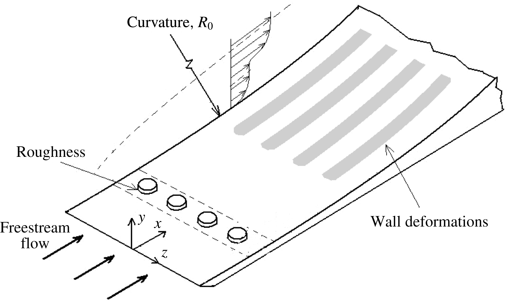
The vortices are initiated by roughness elements placed close to the leading edge in which the local surface is geometrically flat owing to the requirement that $R_{0}\gg O(1)$ (see figure 1). Hence the initial conditions for the transformed BREs are given by the flat-plate case solution as derived in Goldstein et al. (Reference Goldstein, Sescu, Duck and Choudhari2010) (see also the appendix of Sescu & Thompson Reference Sescu and Thompson2015). Equations (2.9)–(2.12) and the associated initial and boundary conditions are marched in the streamwise direction since they are parabolic. To avoid decoupling between the pressure and velocity, a staggered grid is employed in the wall-normal direction, and second-order accurate difference schemes are employed along both $y$ and $z$ directions. The convergence was achieved by a relaxation method, similar to the one employed in Sescu & Thompson (Reference Sescu and Thompson2015).

Figure 1.

Flow configuration sketch.

3 Optimal control problem in the nonlinear regime

While it is common for an optimal flow control problem to be formulated in the framework of a dynamical system (usually, described by a set of equations that are parabolic in time), here we replace the time direction by the $X$ -direction owing to the parabolic character of the BRE in the streamwise direction, which necessitates streamwise marching to obtain a solution. To fix ideas, we first write equations (2.9)–(2.12) in the generic and more compact form

(3.1) $$\begin{eqnarray}\displaystyle {\mathcal{G}}(\boldsymbol{q},\unicode[STIX]{x1D713})=0, & & \displaystyle\end{eqnarray}$$

for brevity, with initial and boundary conditions

(3.2) $$\begin{eqnarray}\displaystyle \boldsymbol{q}(0,Y,z)=\boldsymbol{q}_{0}(Y,z) & & \displaystyle\end{eqnarray}$$

(3.3a,b ) $$\begin{eqnarray}\displaystyle \boldsymbol{q}(X,0,z)=\unicode[STIX]{x1D719},\quad \lim _{Y\rightarrow \infty }\boldsymbol{q}(X,Y,z)=\boldsymbol{q}_{B}(X,z), & & \displaystyle\end{eqnarray}$$

along the wall-normal direction, and periodic or symmetry boundary conditions in the spanwise direction, $z$ . In (3.1), ${\mathcal{G}}()$ is the nonlinear BRE differential operator in abstract notation, $\boldsymbol{q}=(u,v,w,p)$ is the vector of state variables, $\unicode[STIX]{x1D713}$ is the control variable or design parameter that is part of the state equations (in the present case it represents the functional ${\mathcal{F}}(X,z)$ describing the wall deformation), $\unicode[STIX]{x1D719}$ is the control variable associated with the boundary conditions (e.g. the transpiration velocity at the wall, $v_{w}$ ), $\boldsymbol{q}_{0}(Y,z)$ represents the upstream or initial condition in $X=0$ and $\boldsymbol{q}_{B}$ is a given function that specifies the boundary condition at infinity. We define an objective (or cost) functional as

(3.4) $$\begin{eqnarray}\displaystyle {\mathcal{J}}(\boldsymbol{q},\unicode[STIX]{x1D713},\unicode[STIX]{x1D719})={\mathcal{E}}(\boldsymbol{q})+\unicode[STIX]{x1D70E}_{1}(\Vert \unicode[STIX]{x1D713}_{X}\Vert ^{\unicode[STIX]{x1D6FD}_{1}}+\Vert \unicode[STIX]{x1D713}\Vert ^{\unicode[STIX]{x1D6FD}_{1}})+\unicode[STIX]{x1D70E}_{2}(\Vert \unicode[STIX]{x1D719}_{X}\Vert ^{\unicode[STIX]{x1D6FD}_{2}}+\Vert \unicode[STIX]{x1D719}\Vert ^{\unicode[STIX]{x1D6FD}_{2}}), & & \displaystyle\end{eqnarray}$$

where ${\mathcal{E}}(\boldsymbol{q})$ is a specified target function to be minimized (e.g. the energy of the disturbance, or the wall shear stress; the latter is considered in this study), the second and the third terms on the right-hand side of (3.4) are penalization terms depending on the norm of the control variable (usually, these quantities place constraints on the magnitude of the admissible control variables, since they cannot increase or decrease indefinitely), $\unicode[STIX]{x1D70E}_{i}$ and $\unicode[STIX]{x1D6FD}_{i}$ , $i=1,2$ , are given constants and subscript $X$ denotes derivative with respect to $X$ . The norm $\Vert ~\Vert$ in (3.4) is associated with an appropriate inner product of two complex functions, $f$ and $g$ , defined as

(3.5) $$\begin{eqnarray}\displaystyle \langle f,g\rangle =\int _{0}^{X_{t}}f^{\ast }g\,\text{d}X & & \displaystyle\end{eqnarray}$$

in the space $[0,X_{t}]$ , with $X_{t}$ being the terminal streamwise location (the star in (3.5) denotes complex conjugate).

A common approach to transform a (nonlinear) constrained optimization problem into an unconstrained problem is by using the method of Lagrange multipliers (see, for example, Joslin et al. Reference Joslin, Gunzburger, Nicolaides, Erlebacher and Hussaini1997; Gunzburger Reference Gunzburger2000; Zuccher et al. Reference Zuccher, Luchini and Bottaro2004). To this end, we consider the Lagrangian

(3.6) $$\begin{eqnarray}\displaystyle {\mathcal{L}}(\boldsymbol{q},\unicode[STIX]{x1D713},\unicode[STIX]{x1D719},\boldsymbol{q}^{a})={\mathcal{J}}(\boldsymbol{q},\unicode[STIX]{x1D713},\unicode[STIX]{x1D719})-\langle {\mathcal{G}}(\boldsymbol{q},\unicode[STIX]{x1D713}),\boldsymbol{q}^{a}\rangle , & & \displaystyle\end{eqnarray}$$

where $\boldsymbol{q}^{a}$ is the vector of Lagrange multipliers $(u^{a},v^{a},w^{a},p^{a})$ , also known as the adjoint vector. In other words, the Lagrange multipliers are introduced in order to transform the minimization of ${\mathcal{J}}(\boldsymbol{q},\unicode[STIX]{x1D713},\unicode[STIX]{x1D719})$ under the constraint ${\mathcal{G}}(\boldsymbol{q},\unicode[STIX]{x1D713})=0$ into the unconstrained minimization of ${\mathcal{L}}(\boldsymbol{q},\unicode[STIX]{x1D713},\unicode[STIX]{x1D719},\boldsymbol{q}^{a})$ . The unconstrained optimization problem can be formulated as:

Find the control variables $\unicode[STIX]{x1D713}$ and $\unicode[STIX]{x1D719}$ , the state variables $\boldsymbol{q}$ and the adjoint variables $\boldsymbol{q}^{a}$ such that the Lagrangian ${\mathcal{L}}(\boldsymbol{q},\unicode[STIX]{x1D713},\unicode[STIX]{x1D719},\boldsymbol{q}^{a})$ is a stationary function, that is

(3.7) $$\begin{eqnarray}\displaystyle \unicode[STIX]{x1D6FF}{\mathcal{L}}=\frac{\unicode[STIX]{x2202}{\mathcal{L}}}{\unicode[STIX]{x2202}\boldsymbol{q}}\unicode[STIX]{x1D6FF}\boldsymbol{q}+\frac{\unicode[STIX]{x2202}{\mathcal{L}}}{\unicode[STIX]{x2202}\unicode[STIX]{x1D713}}\unicode[STIX]{x1D6FF}\unicode[STIX]{x1D713}+\frac{\unicode[STIX]{x2202}{\mathcal{L}}}{\unicode[STIX]{x2202}\unicode[STIX]{x1D719}}\unicode[STIX]{x1D6FF}\unicode[STIX]{x1D719}+\frac{\unicode[STIX]{x2202}{\mathcal{L}}}{\unicode[STIX]{x2202}\boldsymbol{q}^{a}}\unicode[STIX]{x1D6FF}\boldsymbol{q}^{a}=0, & & \displaystyle\end{eqnarray}$$

where

(3.8) $$\begin{eqnarray}\displaystyle \frac{\unicode[STIX]{x2202}{\mathcal{L}}}{\unicode[STIX]{x2202}a}\unicode[STIX]{x1D6FF}a=\frac{{\mathcal{L}}(a+\unicode[STIX]{x1D716}\unicode[STIX]{x1D6FF}a)-{\mathcal{L}}(a)}{\unicode[STIX]{x1D716}} & & \displaystyle\end{eqnarray}$$

represents directional differentiation in the generic direction $\unicode[STIX]{x1D6FF}a$ . All directional derivatives in (3.7) must vanish, providing different sets of equations:

1. (i) Adjoint BRE equations are obtained by taking the derivative with respect to $\boldsymbol{q}$ ,

   (3.9) $$\begin{eqnarray}\displaystyle \frac{\unicode[STIX]{x2202}{\mathcal{L}}}{\unicode[STIX]{x2202}\boldsymbol{q}}=0\quad \Rightarrow \quad {\mathcal{G}}^{a}(\boldsymbol{q}^{a},\unicode[STIX]{x1D713})=0. & & \displaystyle\end{eqnarray}$$

2. (ii) Optimality conditions are obtained by taking the derivatives with respect to  $\unicode[STIX]{x1D713}$ or  $\unicode[STIX]{x1D719}$ ,

   (3.10a,b ) $$\begin{eqnarray}\displaystyle \frac{\unicode[STIX]{x2202}{\mathcal{L}}}{\unicode[STIX]{x2202}\unicode[STIX]{x1D713}}=0,\quad \frac{\unicode[STIX]{x2202}{\mathcal{L}}}{\unicode[STIX]{x2202}\unicode[STIX]{x1D719}}=0\quad \Rightarrow \quad O(\boldsymbol{q}^{a},\boldsymbol{q},\unicode[STIX]{x1D713},\unicode[STIX]{x1D719})=0. & & \displaystyle\end{eqnarray}$$

3. (iii) The original BRE equations are obtained by taking the derivative with respect to  $\boldsymbol{q}^{a}$ ,

   (3.11) $$\begin{eqnarray}\displaystyle \frac{\unicode[STIX]{x2202}{\mathcal{L}}}{\unicode[STIX]{x2202}\boldsymbol{q}_{a}}=0\quad \Rightarrow \quad {\mathcal{G}}(\boldsymbol{q},\unicode[STIX]{x1D713})=0. & & \displaystyle\end{eqnarray}$$

Equations (3.9)–(3.11) form the optimal control system that can be utilized to determine the optimal states and the control variables. One can note that the stationarity of the Lagrangian with respect to the adjoint variables $\boldsymbol{q}^{a}=(u^{a},v^{a},w^{a},p^{a})$ essentially yields the original state equations, while the stationarity with respect to the state variables $\boldsymbol{q}=(u,v,w,p)$ yields the adjoint equations that depend on the state variables. The relationship between the state variables and the adjoint variables can be expressed by the adjoint identity,

(3.12) $$\begin{eqnarray}\displaystyle \langle {\mathcal{G}}(\boldsymbol{q},\unicode[STIX]{x1D713}),\boldsymbol{q}^{a}\rangle =\langle \boldsymbol{q},{\mathcal{G}}^{a}(\boldsymbol{q}^{a},\unicode[STIX]{x1D713})\rangle +{\mathcal{B}}(\unicode[STIX]{x1D719}), & & \displaystyle\end{eqnarray}$$

where the last term, ${\mathcal{B}}$ , represents a residual from the boundary conditions.

The adjoint BRE equations (see derivation in appendix A) are

(3.13) $$\begin{eqnarray}\displaystyle \frac{\unicode[STIX]{x2202}v^{a}}{\unicode[STIX]{x2202}Y}+{\mathcal{D}}w^{a}=0, & & \displaystyle\end{eqnarray}$$

(3.14) $$\begin{eqnarray}\displaystyle & & \displaystyle -u\frac{\unicode[STIX]{x2202}u^{a}}{\unicode[STIX]{x2202}X}-\hat{v}\frac{\unicode[STIX]{x2202}u^{a}}{\unicode[STIX]{x2202}Y}-w\frac{\unicode[STIX]{x2202}u^{a}}{\unicode[STIX]{x2202}z}+u^{a}\frac{\unicode[STIX]{x2202}u}{\unicode[STIX]{x2202}X}+v^{a}\frac{\unicode[STIX]{x2202}v}{\unicode[STIX]{x2202}X}+w^{a}\frac{\unicode[STIX]{x2202}w}{\unicode[STIX]{x2202}X}-\frac{\unicode[STIX]{x2202}{\mathcal{F}}}{\unicode[STIX]{x2202}X}\left(u^{a}\frac{\unicode[STIX]{x2202}u}{\unicode[STIX]{x2202}Y}+v^{a}\frac{\unicode[STIX]{x2202}v}{\unicode[STIX]{x2202}Y}+w^{a}\frac{\unicode[STIX]{x2202}w}{\unicode[STIX]{x2202}Y}\right)\nonumber\\ \displaystyle & & \displaystyle \quad +\,2G_{\unicode[STIX]{x1D6EC}}uv^{a}-\frac{\unicode[STIX]{x2202}p^{a}}{\unicode[STIX]{x2202}X}+\frac{\unicode[STIX]{x2202}{\mathcal{F}}}{\unicode[STIX]{x2202}X}\frac{\unicode[STIX]{x2202}p^{a}}{\unicode[STIX]{x2202}Y}-\frac{\unicode[STIX]{x2202}^{2}u^{a}}{\unicode[STIX]{x2202}Y^{2}}-{\mathcal{D}}^{2}u^{a}-\frac{\unicode[STIX]{x2202}^{2}{\mathcal{F}}}{\unicode[STIX]{x2202}z^{2}}\frac{\unicode[STIX]{x2202}u^{a}}{\unicode[STIX]{x2202}Y}=0,\end{eqnarray}$$

(3.15) $$\begin{eqnarray}\displaystyle & & \displaystyle -u\frac{\unicode[STIX]{x2202}v^{a}}{\unicode[STIX]{x2202}X}-\hat{v}\frac{\unicode[STIX]{x2202}v^{a}}{\unicode[STIX]{x2202}Y}-w\frac{\unicode[STIX]{x2202}v^{a}}{\unicode[STIX]{x2202}z}+u^{a}\frac{\unicode[STIX]{x2202}u}{\unicode[STIX]{x2202}Y}+v^{a}\frac{\unicode[STIX]{x2202}v}{\unicode[STIX]{x2202}Y}+w^{a}\frac{\unicode[STIX]{x2202}w}{\unicode[STIX]{x2202}Y}-\frac{\unicode[STIX]{x2202}p^{a}}{\unicode[STIX]{x2202}Y}-\frac{\unicode[STIX]{x2202}^{2}v^{a}}{\unicode[STIX]{x2202}Y^{2}}\nonumber\\ \displaystyle & & \displaystyle \quad -\,{\mathcal{D}}^{2}v^{a}-\frac{\unicode[STIX]{x2202}^{2}{\mathcal{F}}}{\unicode[STIX]{x2202}z^{2}}\frac{\unicode[STIX]{x2202}v^{a}}{\unicode[STIX]{x2202}Y}=0,\end{eqnarray}$$

(3.16) $$\begin{eqnarray}\displaystyle & & \displaystyle -u\frac{\unicode[STIX]{x2202}w^{a}}{\unicode[STIX]{x2202}X}-\hat{v}\frac{\unicode[STIX]{x2202}w^{a}}{\unicode[STIX]{x2202}Y}-w\frac{\unicode[STIX]{x2202}w^{a}}{\unicode[STIX]{x2202}z}+u^{a}\frac{\unicode[STIX]{x2202}u}{\unicode[STIX]{x2202}z}+v^{a}\frac{\unicode[STIX]{x2202}v}{\unicode[STIX]{x2202}z}+w^{a}\frac{\unicode[STIX]{x2202}w}{\unicode[STIX]{x2202}z}-\frac{\unicode[STIX]{x2202}{\mathcal{F}}}{\unicode[STIX]{x2202}z}\left(u^{a}\frac{\unicode[STIX]{x2202}u}{\unicode[STIX]{x2202}Y}+v^{a}\frac{\unicode[STIX]{x2202}v}{\unicode[STIX]{x2202}Y}+w^{a}\frac{\unicode[STIX]{x2202}w}{\unicode[STIX]{x2202}Y}\right)\nonumber\\ \displaystyle & & \displaystyle \quad -\,{\mathcal{D}}p^{a}-\frac{\unicode[STIX]{x2202}^{2}w^{a}}{\unicode[STIX]{x2202}Y^{2}}-{\mathcal{D}}^{2}w^{a}-\frac{\unicode[STIX]{x2202}^{2}{\mathcal{F}}}{\unicode[STIX]{x2202}z^{2}}\frac{\unicode[STIX]{x2202}w^{a}}{\unicode[STIX]{x2202}Y}=0,\end{eqnarray}$$

satisfying the initial and boundary conditions

(3.17) $$\begin{eqnarray}\displaystyle & \displaystyle (u^{a},v^{a},w^{a},p^{a})|_{X=X_{t}}=(0,0,0,0)\quad \text{in}~\unicode[STIX]{x1D6FA}, & \displaystyle\end{eqnarray}$$

(3.18) $$\begin{eqnarray}\displaystyle & \displaystyle (u^{a},v^{a},w^{a})|_{\unicode[STIX]{x1D6E4}}=\left\{\begin{array}{@{}ll@{}}(\unicode[STIX]{x1D6FC}(\unicode[STIX]{x1D70F}_{w}-\unicode[STIX]{x1D70F}_{0}),0,0)\quad & \text{for}~X\in [X_{s0},X_{s1}]\\ (0,0,0)\quad & \text{otherwise}\end{array}\right. & \displaystyle\end{eqnarray}$$

and

(3.19) $$\begin{eqnarray}\displaystyle (u^{a},v^{a},w^{a},p^{a})|_{Y\rightarrow \infty }=(0,0,0,0), & & \displaystyle\end{eqnarray}$$

where $\unicode[STIX]{x1D6FC}$ is a constant pre-factor that controls the penalization of the wall shear stress. With the state variables $(u,v,w,p)$ determined from equations (2.9)–(2.12), the adjoint equations (3.13)–(3.16) are linear and parabolic, and can be solved via a marching procedure in the backward direction, starting from the terminal streamwise location, $X_{t}$ , towards the initial streamwise location $X_{0}$ .

The optimality equation for control based on wall transpiration is obtained in the form (see derivation in appendix B)

(3.20) $$\begin{eqnarray}\displaystyle \frac{\unicode[STIX]{x2202}^{2}v_{w}}{\unicode[STIX]{x2202}X^{2}}-v_{w}=\frac{1}{\unicode[STIX]{x1D70E}_{2}}\left(p^{a}+\frac{\unicode[STIX]{x2202}v^{a}}{\unicode[STIX]{x2202}Y}\right), & & \displaystyle\end{eqnarray}$$

satisfying the boundary conditions

(3.21) $$\begin{eqnarray}\displaystyle \frac{\unicode[STIX]{x2202}v_{w}}{\unicode[STIX]{x2202}X}(X_{0})=0,\quad \frac{\unicode[STIX]{x2202}v_{w}}{\unicode[STIX]{x2202}X}(X_{1})=0. & & \displaystyle\end{eqnarray}$$

Given $p^{a}$ and $v^{a}$ from the adjoint equations, equation (3.20) represents a two-point boundary value problem for $X$ inside the interval $[X_{0},X_{1}]$ . The optimality equation for control based on wall deformation is given as (see derivation in appendix C)

(3.22) $$\begin{eqnarray}\displaystyle \unicode[STIX]{x1D70E}_{1}\frac{\unicode[STIX]{x2202}^{2}{\mathcal{F}}}{\unicode[STIX]{x2202}X^{2}}-2\frac{\unicode[STIX]{x2202}u^{a}}{\unicode[STIX]{x2202}z}\frac{\unicode[STIX]{x2202}^{2}u}{\unicode[STIX]{x2202}Y^{2}}\frac{\unicode[STIX]{x2202}{\mathcal{F}}}{\unicode[STIX]{x2202}z}-\unicode[STIX]{x1D70E}_{1}{\mathcal{F}}=\frac{\unicode[STIX]{x2202}^{2}u^{a}}{\unicode[STIX]{x2202}z^{2}}\frac{\unicode[STIX]{x2202}u}{\unicode[STIX]{x2202}Y}-2\frac{\unicode[STIX]{x2202}u^{a}}{\unicode[STIX]{x2202}z}\frac{\unicode[STIX]{x2202}^{2}u}{\unicode[STIX]{x2202}Y\unicode[STIX]{x2202}z}-\frac{\unicode[STIX]{x2202}p^{a}}{\unicode[STIX]{x2202}X}\frac{\unicode[STIX]{x2202}u}{\unicode[STIX]{x2202}Y}-\frac{\unicode[STIX]{x2202}p^{a}}{\unicode[STIX]{x2202}z}\frac{\unicode[STIX]{x2202}w}{\unicode[STIX]{x2202}Y}, & & \displaystyle\end{eqnarray}$$

subject to the boundary conditions

(3.23a,b ) $$\begin{eqnarray}\displaystyle \frac{\unicode[STIX]{x2202}{\mathcal{F}}}{\unicode[STIX]{x2202}X}(X_{0})=0,\quad \frac{\unicode[STIX]{x2202}{\mathcal{F}}}{\unicode[STIX]{x2202}X}(X_{1})=0. & & \displaystyle\end{eqnarray}$$

Again, equation (3.22) represents a two-point boundary value problem for $X$ inside the interval $[X_{0},X_{1}]$ , but unlike the optimality condition associated with the wall transpiration that depends only on adjoint variables, this equation also depends on state variables, $u$ and $w$ , and their derivatives. The constant pre-factors $\unicode[STIX]{x1D70E}_{1}$ and $\unicode[STIX]{x1D70E}_{2}$ are used to control the importance of the terms they multiply in (A 1).

Alternatively, the optimality condition (3.20) or (3.22) can be replaced by a gradient method or steepest descent method, wherein the objective function is updated according to

(3.24) $$\begin{eqnarray}\displaystyle {\mathcal{F}}^{(n+1)}={\mathcal{F}}^{(n)}-\unicode[STIX]{x1D6FC}\frac{\text{d}{\mathcal{J}}^{(n)}}{\text{d}{\mathcal{F}}^{(n)}} & & \displaystyle\end{eqnarray}$$

for control based on wall deformations, or

(3.25) $$\begin{eqnarray}\displaystyle v_{w}^{(n+1)}=v_{w}^{(n)}-\unicode[STIX]{x1D6FC}\frac{\text{d}{\mathcal{J}}^{(n)}}{\text{d}v_{w}^{(n)}} & & \displaystyle\end{eqnarray}$$

for control based on wall transpiration, where $n$ represent the iteration index, and $\unicode[STIX]{x1D6FC}$ in this case is the descent parameter (note that the results in this study are obtained based on solving the optimality equations (3.20) and (3.22)).

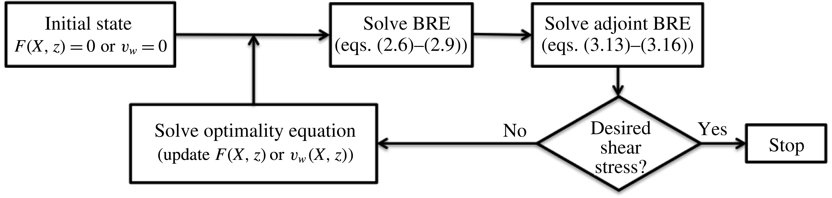
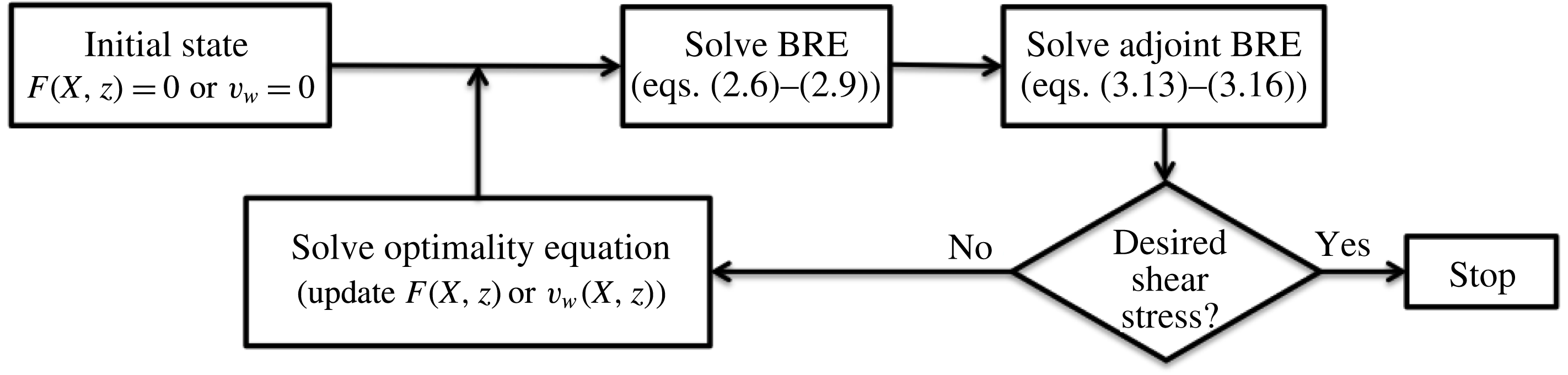
The optimal control procedure based on wall transpiration or deformation is shown schematically in figure 2. The control algorithm starts with the solution to BRE for the uncontrolled boundary layer, followed by the solution to the adjoint BRE (note that the adjoint BRE depends on the solution to the BRE). The difference between the wall shear stress and the Blasius wall shear stress is then compared to a desired value; if the difference is larger than a given threshold then the optimality condition equation is solved to determine the new wall shape ${\mathcal{F}}$ , or the new wall transpiration velocity $v_{w}$ . Once these are determined, the loop is repeated, and the calculation finishes when the difference between the wall shear stress and the desired value is less than the threshold.

Figure 2.

Schematic of the control algorithm steps.

Adjoint equations (3.13)–(3.16) and the associated initial and boundary conditions (3.17)–(3.19) are solved numerically on the same grid as the original BRE state equations (2.9)–(2.12), and utilizing the same numerical algorithm (as for the BRE equations), except that the marching is preformed backwards, starting from the terminal streamwise location. The optimality equations (3.20) and (3.22) and the associated boundary conditions (3.21) and (3.23) respectively, are solved via a Jacobi relaxation method.

4 Results and discussion

4.1 Preliminaries

A row of roughness elements located at a fixed distance of 0.5 m from the leading edge (see figure 1) is considered for the spanwise separation distances $\unicode[STIX]{x1D6EC}^{\ast }=0.8$ , 1.2 and 1.6 cm. The effect of roughness elements on the boundary layer is not directly modelled, but taken into account by imposing initial conditions derived in Goldstein et al. (Reference Goldstein, Sescu, Duck and Choudhari2010) through asymptotic analysis under the assumption that the roughness height is asymptotically small and the Reynolds number is large. The Görtler number based on spanwise separation is $G_{\unicode[STIX]{x1D6EC}}=318\,887$ (corresponding to a Görtler number based on the momentum displacement thickness of 6.428). The functional form describing the roughness element is given by the localized function $\exp [-(x^{2}+z^{2})/(D/2)^{2}]$ , where $D$ represents the diameter of the roughness element. The kinetic energy associated with the Görtler vortex is calculated according to

(4.1) $$\begin{eqnarray}\displaystyle E(X)=\int _{z_{1}}^{z_{2}}\int _{0}^{\infty }[|v-v_{m}(X,y)|^{2}+|w-w_{m}(X,y)|^{2}+|u-u_{m}(X,y)|^{2}]\,\text{d}z\,\text{d}y, & & \displaystyle\end{eqnarray}$$

where $u_{m}(X,y)$ , $v_{m}(X,y)$ and $w_{m}(X,y)$ are the spanwise mean components of velocity, and $z_{1}$ and $z_{2}$ are the boundary limits in the spanwise direction, while the spanwise averaged wall shear stress given by

(4.2) $$\begin{eqnarray}\displaystyle \unicode[STIX]{x1D70F}_{w}(X)=\frac{1}{(z_{2}-z_{1})}\int _{z_{1}}^{z_{2}}\frac{\unicode[STIX]{x2202}u}{\unicode[STIX]{x2202}Y}(X,0,z)\,\text{d}z, & & \displaystyle\end{eqnarray}$$

where, as mentioned earlier, the shape of the wall is taken into account implicitly through the partial derivative with respect to $Y$ .

In the results that follow, control is applied using either wall deformation or wall transpiration by an iterative procedure as described in the previous section. In the case of wall transpiration, the cumulative blowing or suction at the wall is realized such that a zero mass flow rate is maintained to avoid injecting or absorbing mass into/from the flow. The efficiency of the control is quantified through results consisting of streamwise velocity contours, streamwise distribution of the energy of the disturbances and of the spanwise averaged wall shear stress.

Figure 3.

Energy (a) and the spanwise averaged wall shear stress (b) calculated using four different grids ( $\unicode[STIX]{x1D6EC}^{\ast }=1.2$  cm).

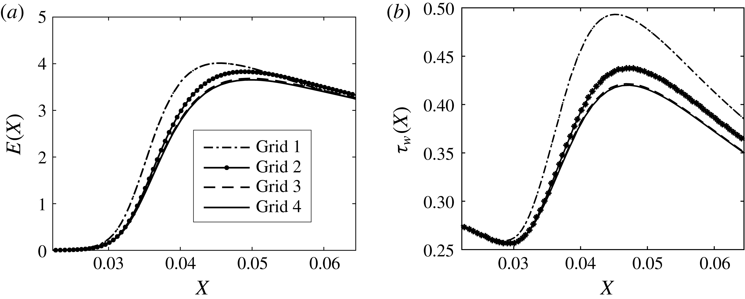
To ensure that the numerical results are accurate, a grid study is performed to determine the appropriate number of grid points along the wall-normal and spanwise directions. To this end, we consider four grid resolutions, consisting of 21, 31, 41 and 51 points in the spanwise direction, and 141, 161, 181 and 201 points in the wall-normal direction, while the number of grid points in the streamwise direction was fixed at 300, corresponding to a spatial step of $\unicode[STIX]{x0394}X=2.222\times 10^{-4}$ . To reduce the computational cost, the domain size in the spanwise direction has been reduced to half the distance between two roughness elements, with symmetry conditions – instead of periodic conditions – applied at the right and left boundaries. Results in terms of energy of the disturbance and spanwise averaged shear stress distributions in the streamwise direction are plotted in figure 3 for all four grids. The solution converges to a final state as the number of grid points is increased (the convergence is measured by the relative energy error between two iterations, which was set at $10^{-3}$ ). 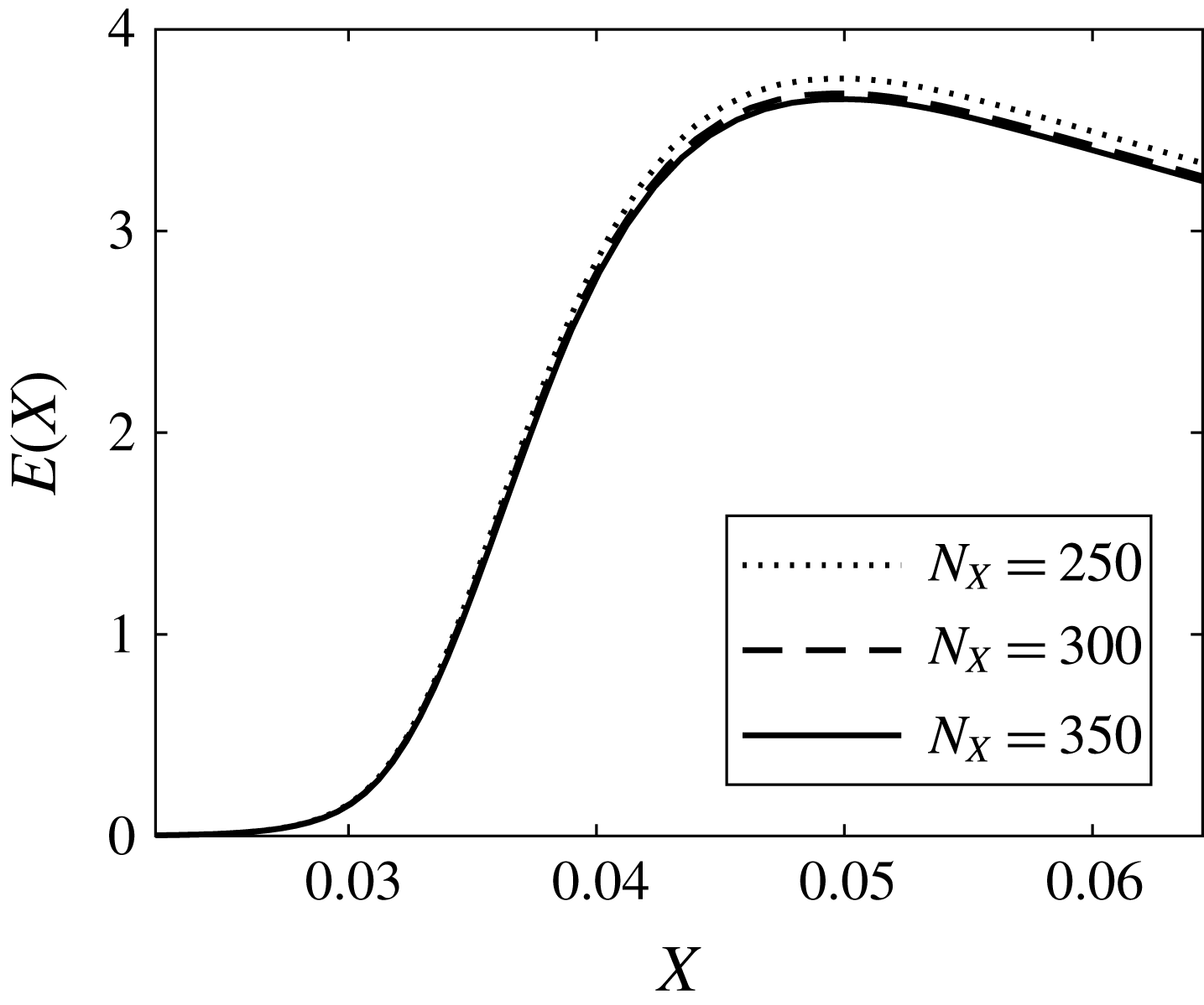As a result of the grid study, the resolution associated with ‘grid 3’, consisting of $41\times 181$ points in the spanwise and wall-normal directions respectively, was chosen for subsequent calculations. The numerical solution was found to be less sensitive to the resolution in the streamwise direction because a sufficiently large number of grid points was chosen (appendix D shows a comparison between three resolutions).

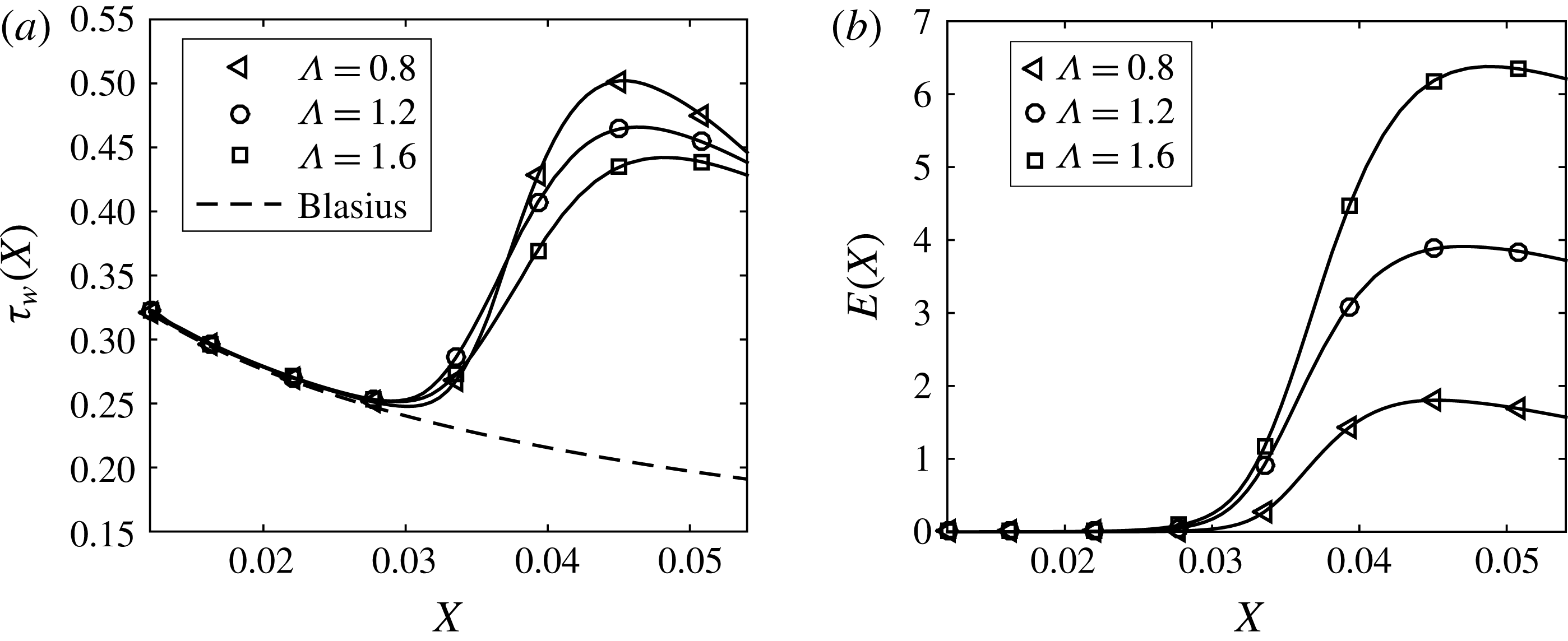
Before presenting results from the control schemes, in figure 4, we show the effect of varying the spanwise separation on the vortex energy growth (a) and on the spanwise averaged wall shear stress (b) for the uncontrolled boundary layer. It is seen that while the wall shear stress is not substantially affected, the energy of the disturbance seems to show a significant variation.

Figure 4.

Spanwise averaged wall shear stress (a) and energy (b) as a function of the streamwise direction and for different roughness spanwise separations ( $\unicode[STIX]{x1D6EC}^{\ast }=1.2$  cm).

Figure 5.

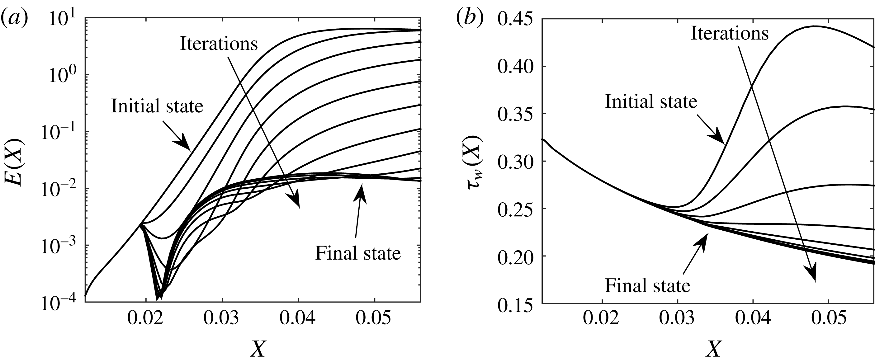
Typical convergence of the control algorithm: (a) energy; (b) spanwise averaged wall shear stress ( $\unicode[STIX]{x1D6EC}^{\ast }=1.2$  cm).

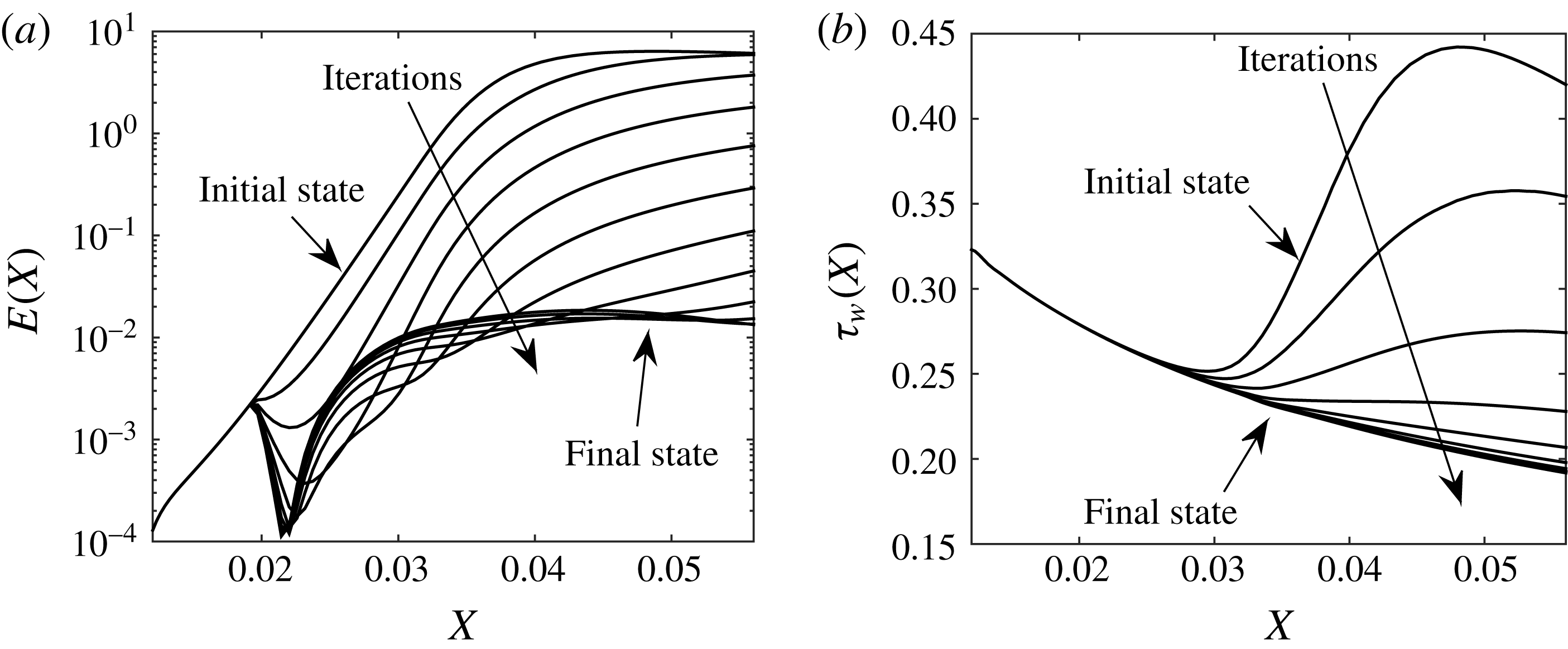
In the following subsections, the interval where the control is applied, $[X_{0},X_{1}]$ , and the interval where the cost function is defined, $[X_{s0},X_{s1}]$ , are the same; the downstream boundary of both intervals coincides with the terminal location $X_{t}$ . To illustrate the control iterations and its convergence, figure 5 shows the energy of the disturbance (a) and the spanwise averaged wall shear stress (b) for a control algorithm based on wall deformations; for this particular case, approximately 12 iterations were necessary to obtained the optimum wall deformation that provides the lowest wall shear stress (the total number of iterations depends on the parameters $\unicode[STIX]{x1D70E}_{1}$ and $\unicode[STIX]{x1D70E}_{2}$ in (3.4)). The boundary layer was excited by a row of periodic roughness elements (the roughness elements are located in $x^{\ast }=0.5$  m from the leading edge, the spanwise separation is 1.2 cm and $X_{0}=0.015$ ). The initial state curve in figure 5 corresponds to the energy associated with the uncontrolled Görtler vortices, while the final state curve represents the optimum wall deformation. More than three orders of magnitude reduction in the energy was attained for this particular case. An exponential convergence for the first several steps can be observed in figure 5(a), where the energy increment in the logarithmic scale from one iteration to the next seems to be constant. The shear stress plot on the right (panel b) shows that in 5–6 iterations the level of the frictional drag can be reduced considerably (the final state is remarkably very close to the shear stress corresponding to the original Blasius solution, as will be shown in the subsequent figures).

4.2 Sensitivity to control location, $X_{0}$

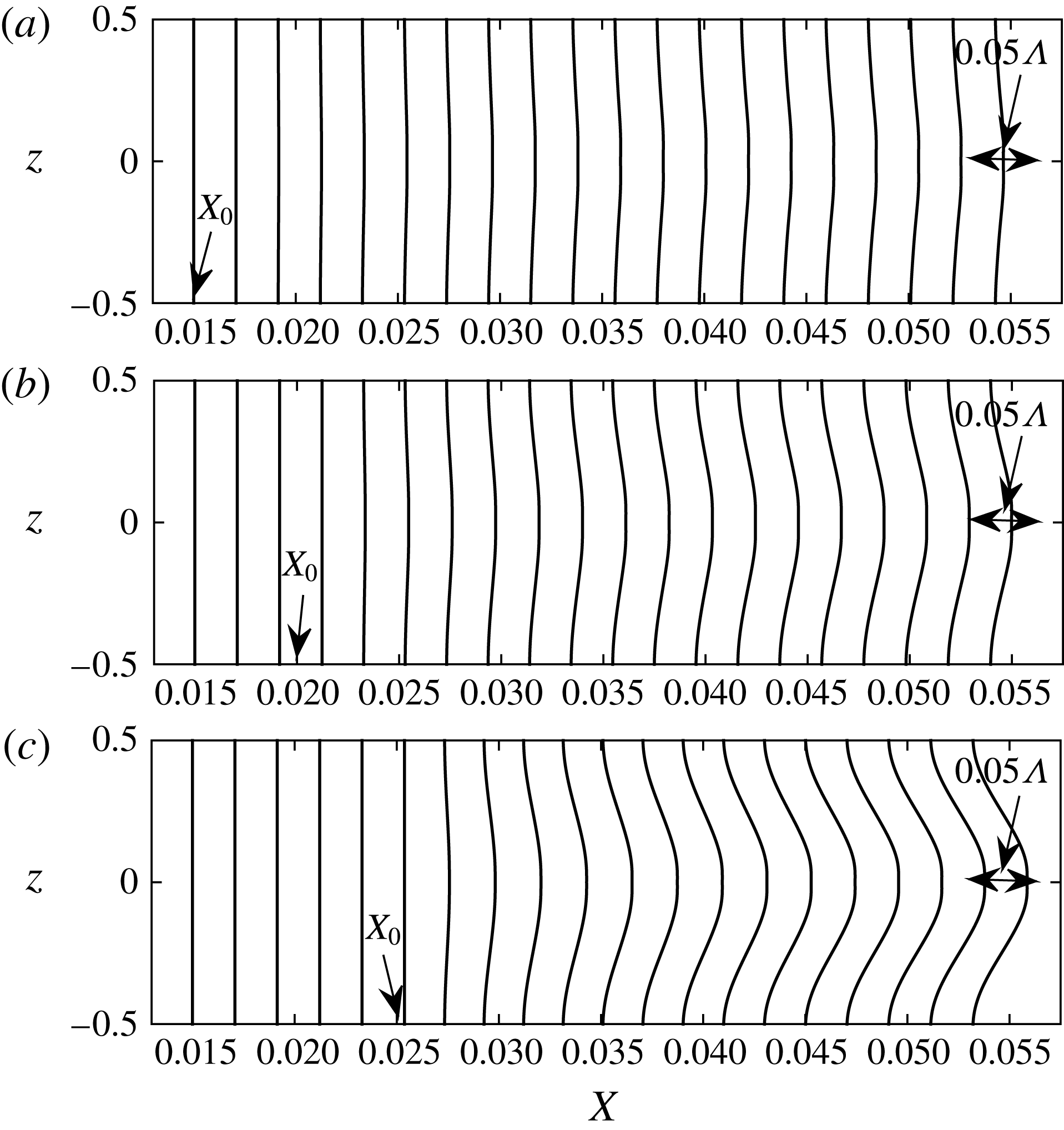
In this section, we show results for the optimal control applied to three different values of $X_{0}$ , which corresponds to the location where the control is initiated. Both types of control, wall deformation and transpiration, are analysed here, and results for spanwise separation of $\unicode[STIX]{x1D6EC}^{\ast }=1.2$ cm are presented and discussed. The wall displacement as a consequence of the control based on wall deformations is plotted in figure 6 at different streamwise locations, and for all three values of $X_{0}$ . They represent distributions of the wall displacement along the spanwise direction at equal streamwise increments starting from $X=0.015$ to $X=0.055$ . It appears that the amplitude of the wall displacement is highly dependent on $X_{0}$ , and that the displacement is a small percentage of the boundary layer thickness (the maximum is approximately 5 %, which corresponds to the largest value of $X_{0}$ ). For the smallest value of $X_{0}$ , the maximum wall displacement is below 1 %, which can be considered negligible in the calculation of the integrated frictional drag (i.e. there is no considerable increase in the surface area due to the wall displacement). These results suggest that as the energy of the Görtler vortex increases with the streamwise coordinate it becomes more difficult to control the flow using wall deformations.

Figure 6.

The displacement of the wall represented by profiles in the $z$ -direction, for the spanwise separation $\unicode[STIX]{x1D6EC}^{\ast }=1.2$  cm and different control initiation locations: (a) $X_{0}=0.015$ ; (b) $X_{0}=0.02$ ; (c) $X_{0}=0.025$ .

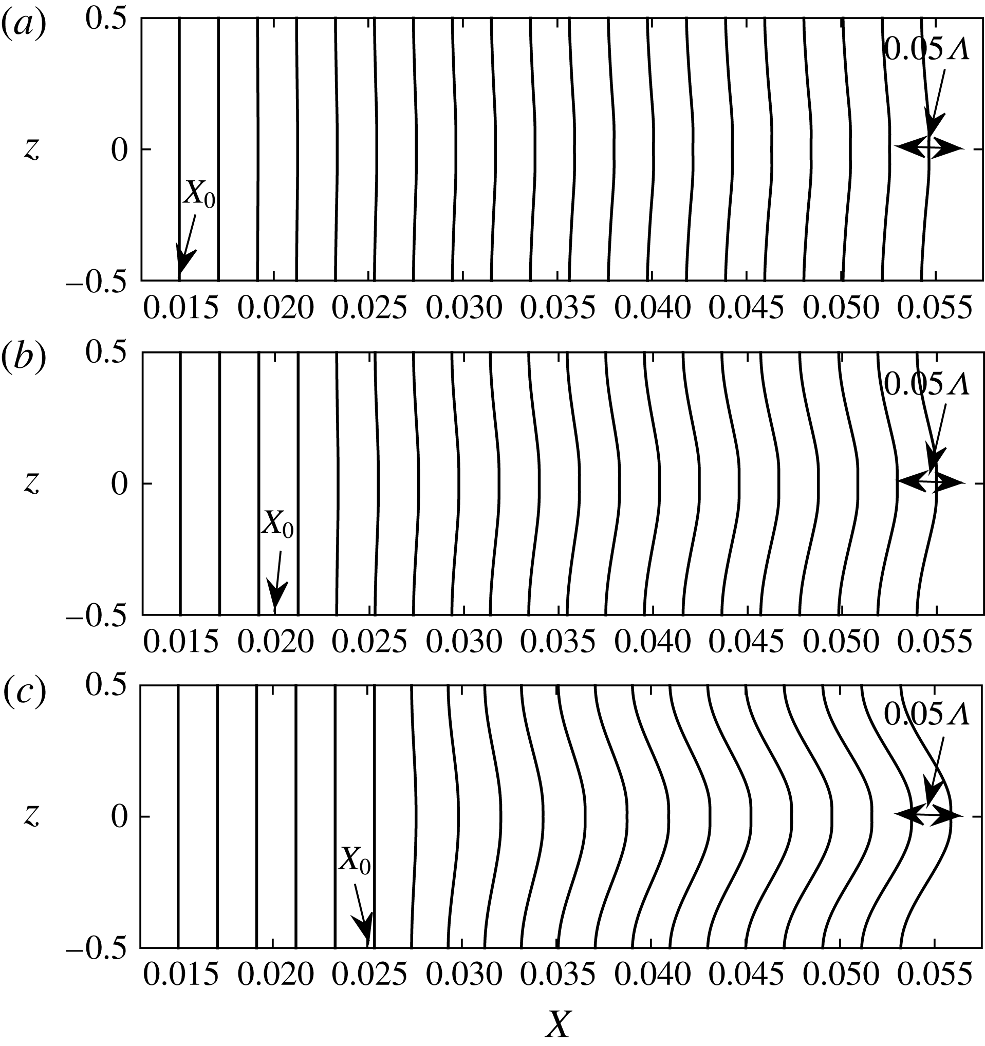
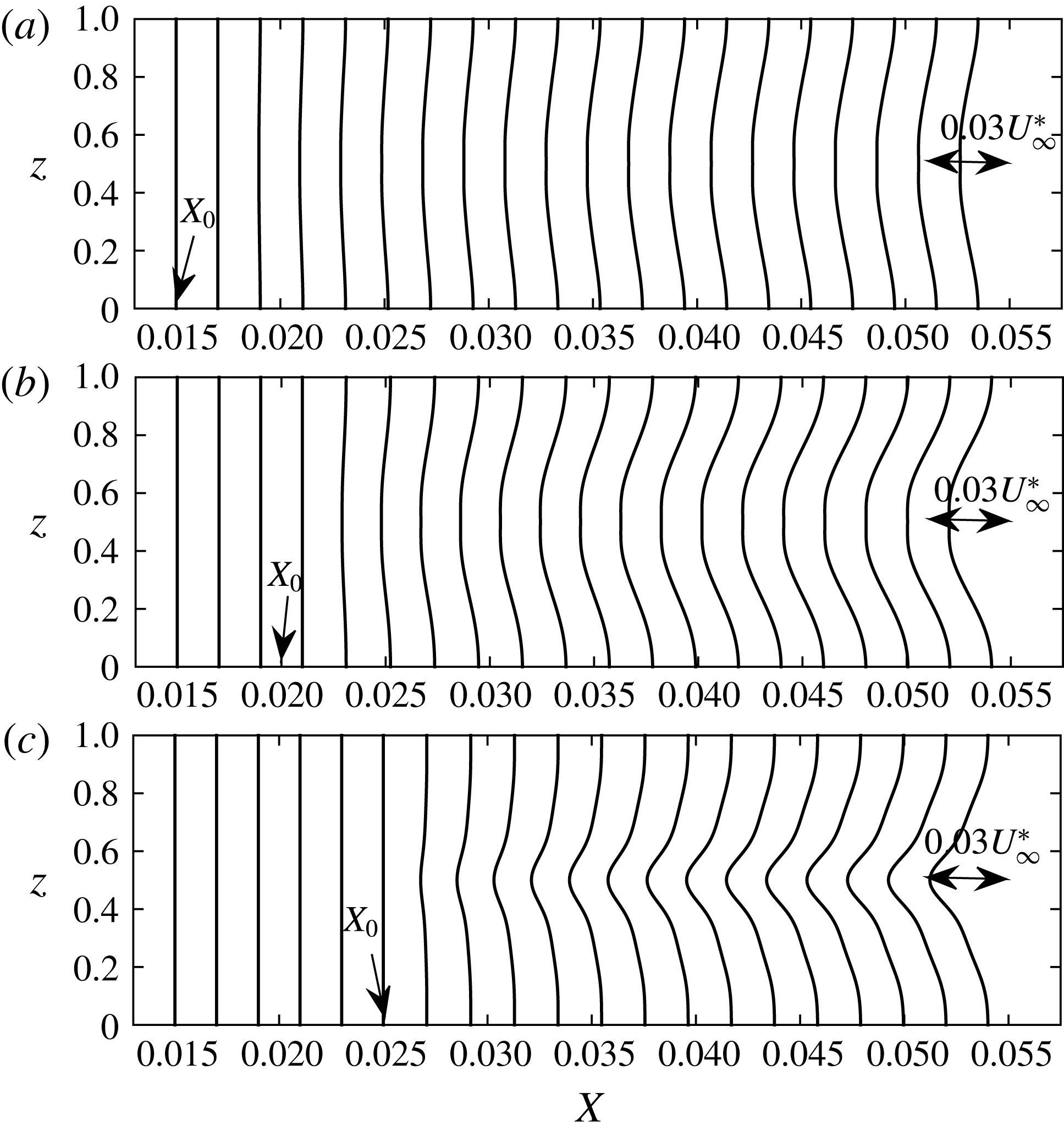
Similar distribution of curves for different values of $X_{0}$ are included in figure 7, except the wall transpiration velocity is plotted along the spanwise direction. As the control initiation location is moved downstream, the magnitude of the transpiration velocity is increased, which is to be expected because the streak strength (defined as the difference between the high speed and the low speed in the streaks) increases in the streamwise direction, demanding more momentum injection or suction from the wall. It will be shown in the next contour plots that moving the initiation location in the downstream is not as effective in reducing the energy of the vortices as the control based on wall deformations. The maximum transpiration velocity attained in the downstream for $X_{0}=0.025$ is a small percentage from the free-stream velocity (3 %); it is a much smaller percentage for $X_{0}=0.015$ (less than 1 %).

Figure 7.

The distribution of transpiration velocity, $v_{w}/V_{\infty }$ , at the wall represented by profiles in the spanwise $z$ -direction, for the spanwise separation $\unicode[STIX]{x1D6EC}^{\ast }=1.2$  cm and different control initiation locations: (a) $X_{0}=0.015$ ; (b) $X_{0}=0.02$ ; (c) $X_{0}=0.025$ .

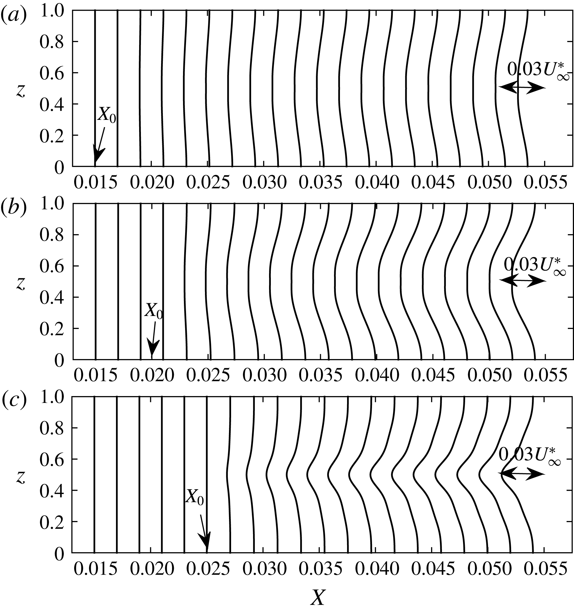
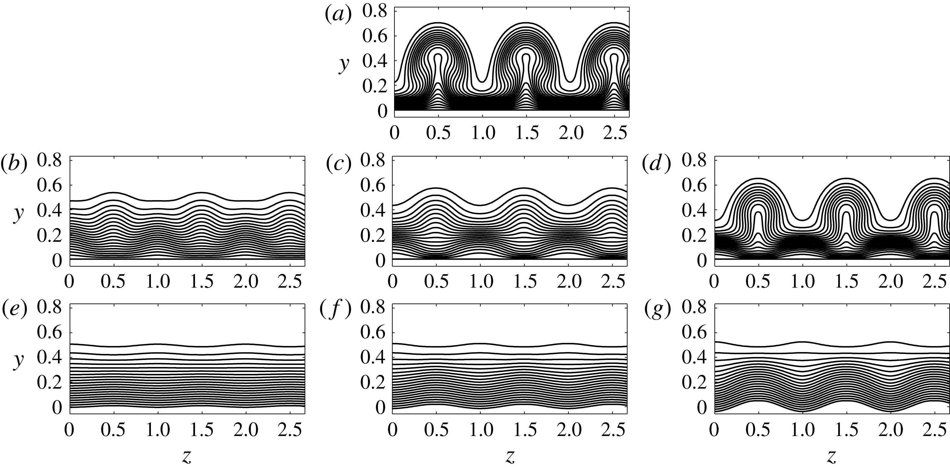
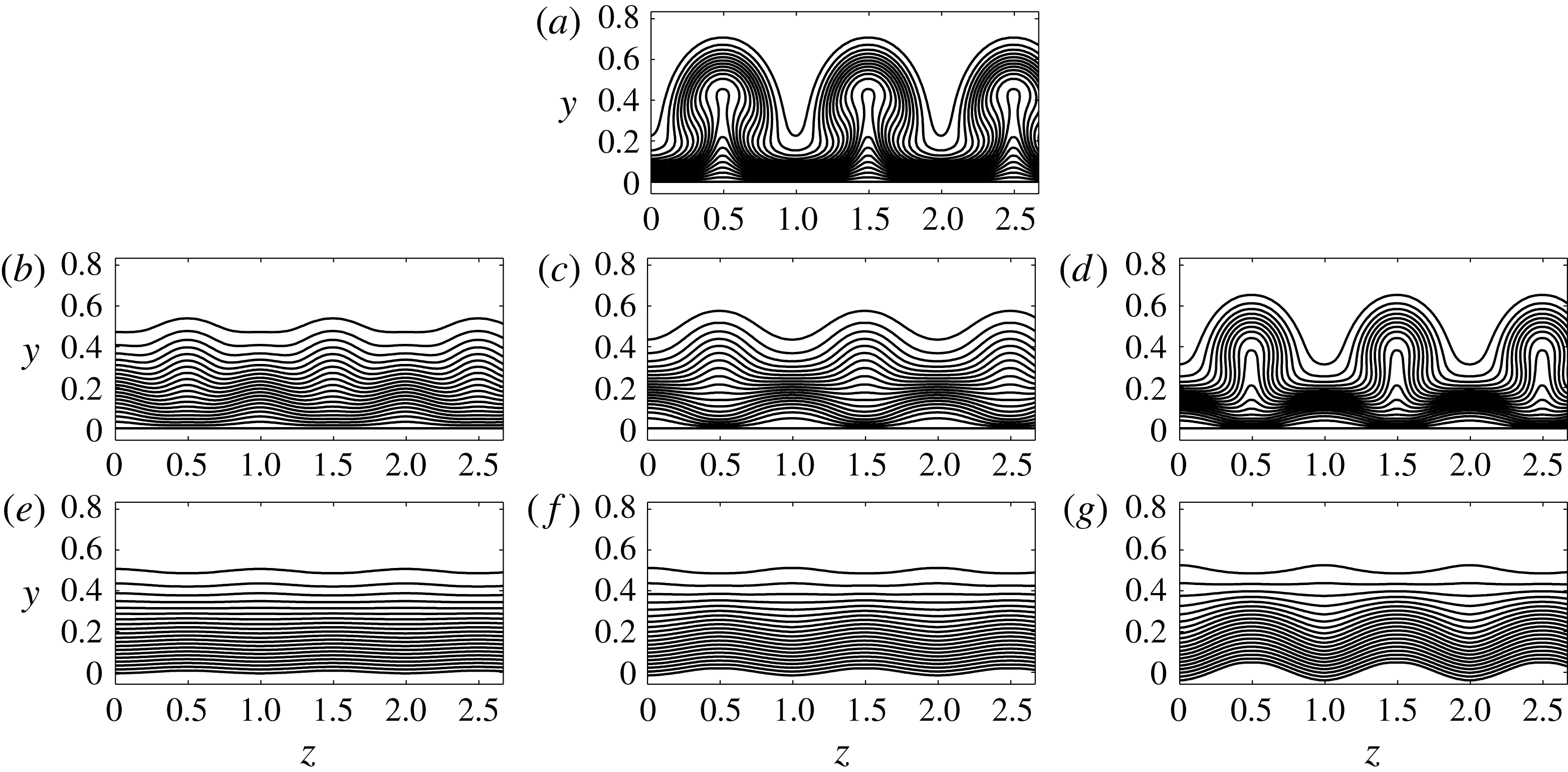
Regions of low and high speed associated with the streak can be visualized by plotting contours of streamwise velocity in sections at the fixed streamwise location $X=0.04$ , as shown in figure 8. Görtler vortices developing in the uncontrolled case (figure 8 a) reveal fully developed ‘mushroom‘ shapes with alternating low-speed streaks and high-speed streaks in the spanwise direction. Panels b, c and d of figure 8 correspond to results obtained by applying the control based on wall transpiration, while the right column of plots (panels 8 e, f and g) corresponds to results obtained by applying wall deformations. In the control algorithm based on wall deformations, the wall surface is gradually moved upward at the spanwise location corresponding to the low-speed streak, while at the same time it is moved downward at the spanwise location corresponding to high-speed streaks. This change in the geometry of the wall surface increases or decreases the momentum of the flow, thus reducing the energy associated with the Görtler vortices. The same mechanism is at play when wall transpiration is applied, except that the upward motion of the wall is replaced by blowing and the downward motion by suction. These contours show that the control based on wall deformations is more effective than the control based on wall transpiration, especially at high control initiation location $X_{0}=0.025$ . The difference between the results from the two control schemes is qualitatively measured from the contour plots by comparing the level of spanwise variation; for example, by comparing figure 8(b,c) it is noted that there are significant spanwise variations of the contour lines on the left-hand side (corresponding to the control based on wall transpiration), while on the right-hand side the flow appears as a Blasius boundary layer; more quantitative results will be shown in plots of energy and wall shear stress later in the section. Note that previously, it was found that the control based on wall transpiration is more effective than control based on wall deformation in wall turbulence (see, for example, Endo et al. Reference Endo, Kasagi and Suzuki2000, Kang & Choi Reference Kang and Choi2000). However, the comparison of our results with the control of wall turbulence is largely irrelevant since the physics of the flow is different; moreover, here we target steady Görtler vortices, where the streamwise gradients are neglected, while a turbulent boundary layer is highly unsteady with strong variations of the flow in the streamwise direction. Another reason is that for our problem a parabolic set of equations is solved in a pre-transitional boundary layer, where there is no feedback to the downstream flow, and the variation of the wall deformation with respect to the streamwise direction is rather gentle (versus the variation in the spanwise direction). A thorough discussion of the physical mechanism and interpretations behind both types of control algorithms is presented later in § 5.

Figure 8.

Streamwise velocity contours for spanwise separation $\unicode[STIX]{x1D6EC}^{\ast }=1.2$  cm, at the streamwise location $X=0.04$ : (a) no control; (b) control based on wall transpiration, $X_{0}=0.015$ ; (c) control based on wall transpiration, $X_{0}=0.02$ ; (d) control based on wall transpiration, $X_{0}=0.025$ ; (e) control based on wall deformation, $X_{0}=0.015$ ; (f) control based on wall deformation, $X_{0}=0.02$ ; (g) control based on wall deformation, $X_{0}=0.025$ . The contour lines range from 0 at the wall to 1 in the external flow, with an increment of 0.05.

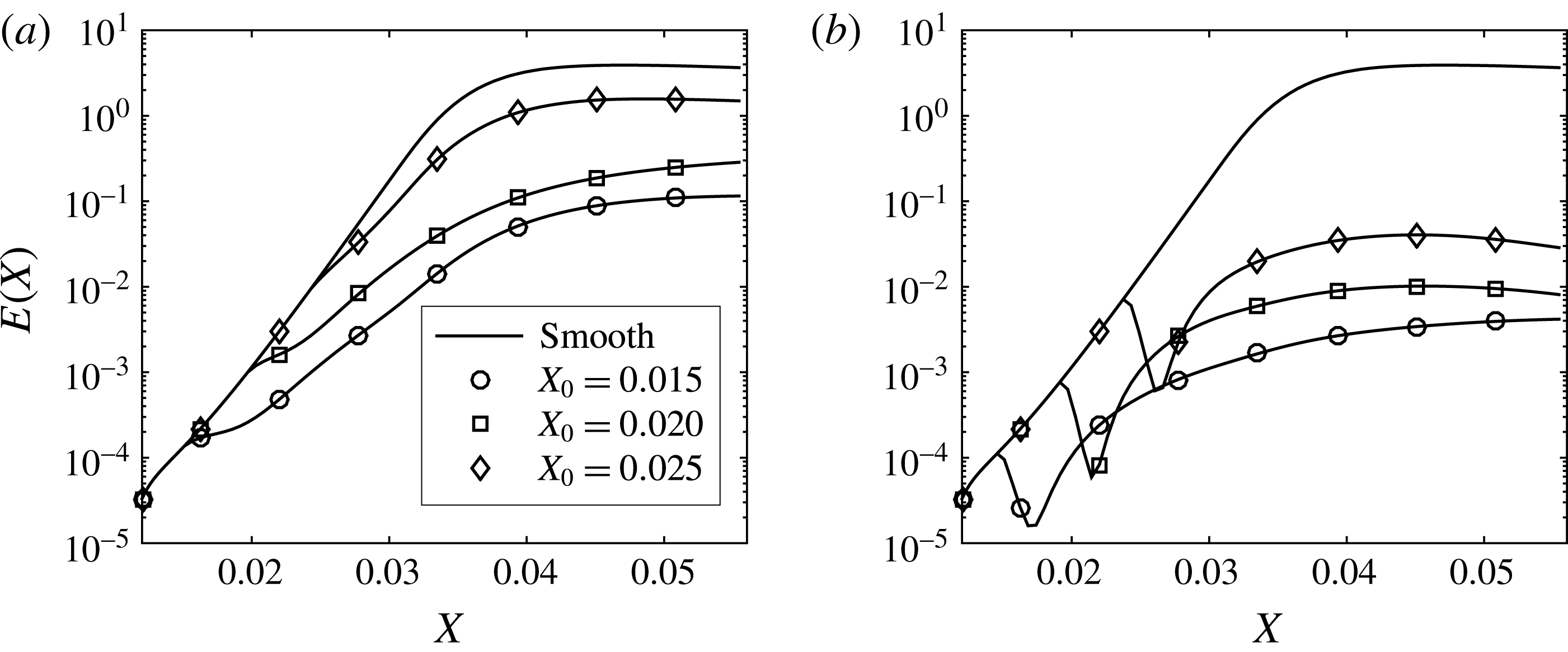
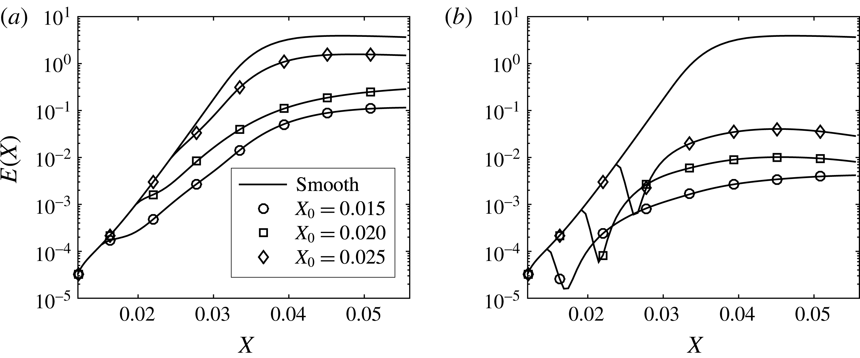
In figure 9, we compare the kinetic energy associated with the Görtler vortex for the three control cases to the energy calculated in the uncontrolled case. The energy is significantly reduced by the control based on wall deformation; for the smallest $X_{0}$ location, an approximately three orders of magnitude reduction is observed. 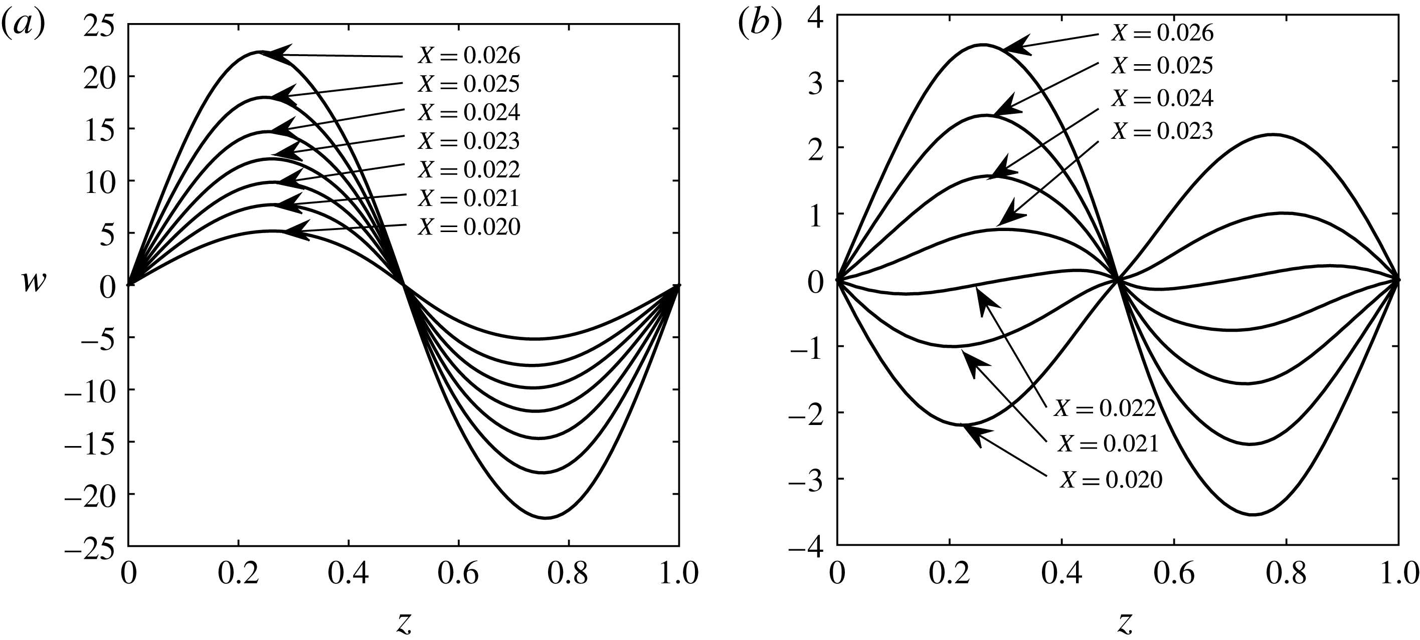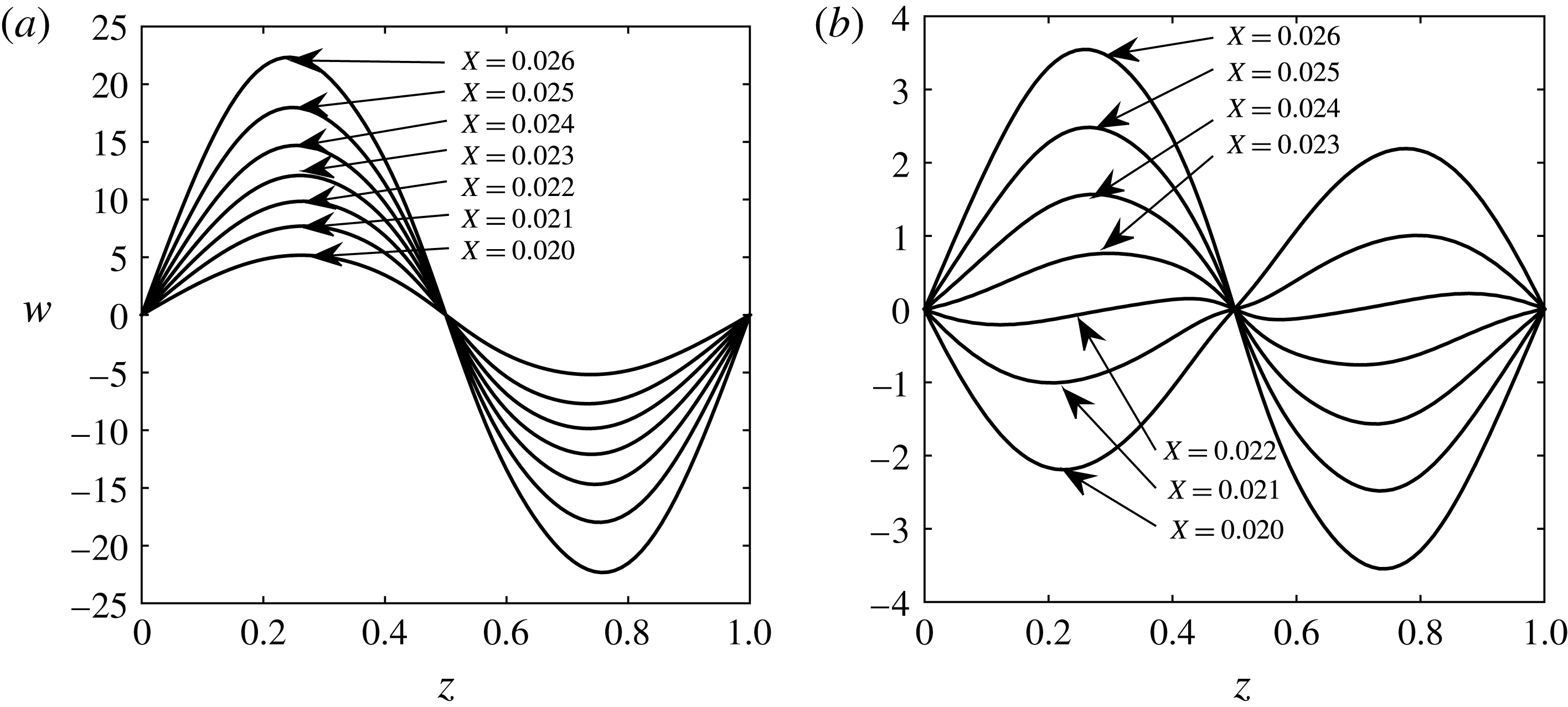The energy reduction in the case of wall transpiration is not as high as in the previous case, but it is considerable at least for the largest $X_{0}$ (almost two orders of magnitude). In figure 9(b), sharp minima in all energy curves associated with the controlled cases exist. These minima correspond to the streamwise location where the low- and high-speed regions switch spanwise locations, and also to the initiation point for the transient energy growth. To further rationalize this behaviour, in figure 10 we plot distributions of the spanwise velocity component, $w$ , as a function of $z$ for several streamwise locations (some upstream and some downstream of the energy minima locations) at $Y=0.07$ from the wall (at the point where $w$ has a maximum in the wall-normal direction). These plots correspond to the energy curve with square symbols in figure 9 ( $X_{0}=0.020$ ), for which the energy minimum occurs at approximately $X=0.022$ . The left-hand figure corresponds to the control based on wall transpiration. We see here that both the positive and negative regions of $w$ are monotonically increasing (in the absolute value). For the control based on wall deformation on the right-hand side on the other hand, there is a sign switch in both positive and negative regions. Since the curve corresponding to $X=0.022$ is the closest to the $w=0$ line, plots in figure 10 indicate that the streamwise location where the energy minimum occurs in figure 9 corresponds to vortices that experience region switching.

Figure 9.

Energy as a function of the streamwise direction for $\unicode[STIX]{x1D6EC}^{\ast }=1.2$  cm: (a) control based on wall transpiration; (b) control based on wall deformations.

Figure 10.

Spanwise velocity component, $w$ , as a function of $z$ for several streamwise locations: (a) control based on wall transpiration; (b) control based on wall deformation ( $\unicode[STIX]{x1D6EC}^{\ast }=1.2$  cm).

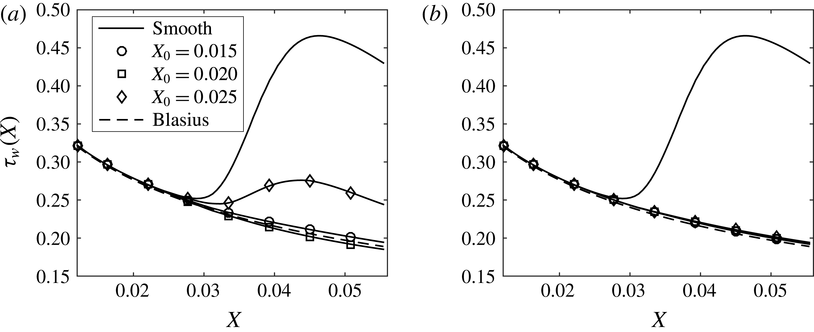
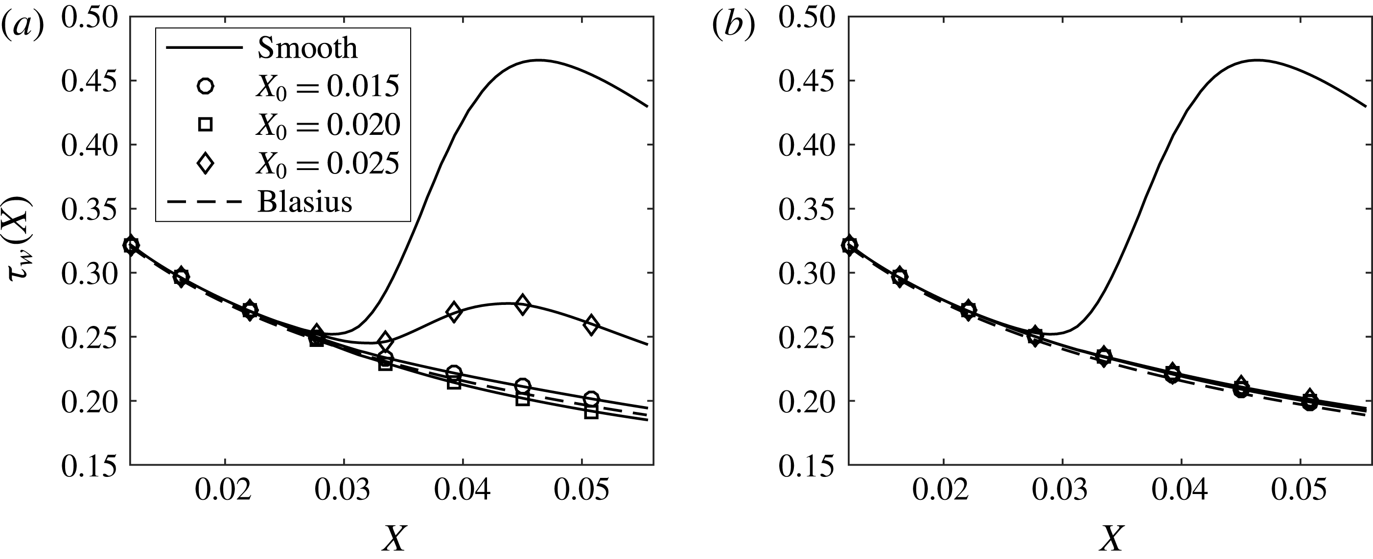
As a means to quantify the effect of control algorithms on the frictional drag, in figure 11 we plot the spanwise averaged wall shear stress for all cases, including the curve corresponding to the Blasius solution (i.e. no Görtler vortices, and no control). First, it appears that there is a significant increase in the shear stress from approximately $X=0.032$ , for Görtler vortices in the uncontrolled case, which translates into an increase in the skin friction drag. It is obvious that the shear stress is significantly reduced by the application of either control scheme, with wall deformations being more effective; this confirms our previous results in figures 4, 5 and 8. The shear stress curves corresponding to the control based on wall deformations (figure 11 b) are all remarkably close to the Blasius curve.

Figure 11.

Spanwise averaged wall shear stress as a function of the streamwise direction for $\unicode[STIX]{x1D6EC}^{\ast }=1.2$  cm: (a) control based on wall transpiration; (b) control based on wall deformations.

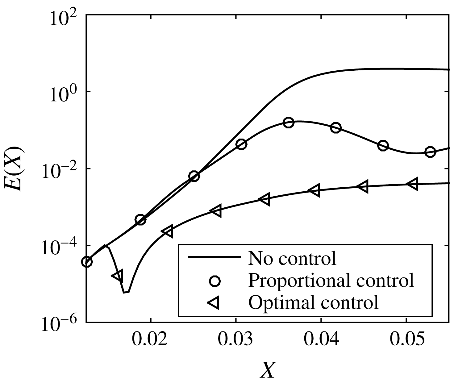
It is interesting to compare the energy plot obtained from the proportional control scheme that was applied in Sescu et al. (Reference Sescu, Taoudi and Afsar2017) with the present energy result, for the same spanwise separation of $\unicode[STIX]{x1D6EC}^{\ast }=1.2$  cm. This is accomplished in figure 12, which shows that the energy reduction corresponding to the optimal control is much more significant than the energy reduction corresponding to the proportional controller. This is not at all surprising, however, since the latter is based on a formulation in which the energy reduction would always be sub-optimal.

Figure 12.

Comparison of energy plot from Sescu et al. (Reference Sescu, Taoudi and Afsar2017) with the present result, for the same spanwise separation $\unicode[STIX]{x1D6EC}^{\ast }=1.2$  cm.

4.3 Sensitivity to the roughness spanwise separation and diameter

In this section, results from three different spanwise separations, $\unicode[STIX]{x1D6EC}^{\ast }=0.8$ , 1.2 and 1.6 cm (where the roughness diameter is fixed at $D=0.6$ ), and three different roughness diameters, $D=0.4$ , 0.7 and 1.0 (where the roughness spanwise separation is fixed at $\unicode[STIX]{x1D6EC}^{\ast }=1.2$ ), are compared to each other. Based on the results from the previous subsection, the control initiation location $X_{0}=0.015$ has been chosen since this provided the best results in terms of both energy and shear stress distributions. Streamwise velocity component contours in the cross-plane at $X=0.04$ are shown in figures 13–15 for the uncontrolled and controlled vortices. Different levels of reductions in the streak amplitude are revealed by these contour plots: for the control based on wall deformations the variations in the spanwise direction are almost absent. The effect of varying the roughness diameters was less noticeable in the contour plots of the streamwise velocity, so they are not shown here.

Figure 13.

Streamwise velocity contours for $X_{0}=0.015$ and $\unicode[STIX]{x1D6EC}^{\ast }=0.8$  cm: (a) no control; (b) control based on wall transpiration; (c) control based on wall deformation. The contour lines range from 0 at the wall to 1 in the external flow, with an increment of 0.05.

Figure 14.

Streamwise velocity contours for $X_{0}=0.015$ and $\unicode[STIX]{x1D6EC}^{\ast }=1.2$  cm: (a) no control; (b) control based on wall transpiration; (c) control based on wall deformation. The contour lines range from 0 at the wall to 1 in the external flow, with an increment of 0.05.

Figure 15.

Streamwise velocity contours for $X_{0}=0.015$ and $\unicode[STIX]{x1D6EC}^{\ast }=1.6$  cm: (a) no control; (b) control based on wall transpiration; (c) control based on wall deformation. The contour lines range from 0 at the wall to 1 in the external flow, with an increment of 0.05.

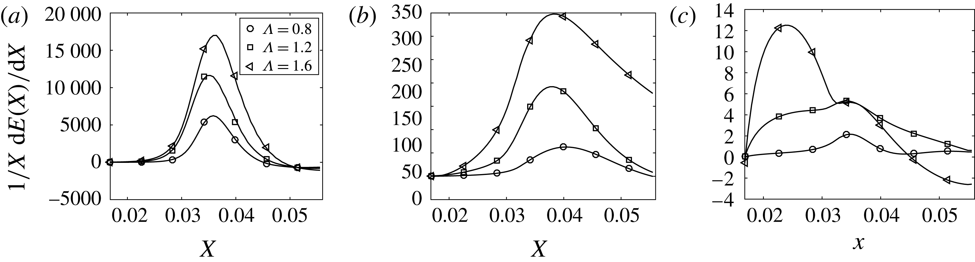
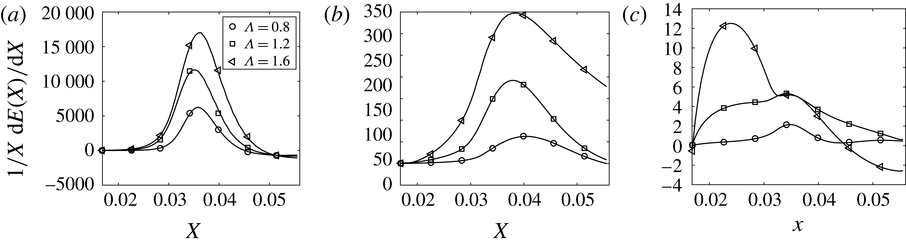
To better highlight the difference among various control cases, the growth rate of energy, $1/X\,\text{d}E/\text{d}X$ , is plotted here, as opposed to the energy itself as was done in the previous subsection. In figure 16 we plot the energy growth rate for different spanwise separations. One noticeable thing inferred from all cases, including the uncontrolled one, is that as the spanwise separation is increased, the energy growth rate is increased, which is altogether expected because the wakes are less likely to coalesce for the largest spanwise separation. The smallest growth rates correspond to the control based on wall deformations as expected (see figure 16 c), being reduced to almost zero for the smallest spanwise separation (circles in figure 16 c). Small energy growth rate is also seen in the case of control based on wall transpiration for the smallest spanwise separation case (circles in figure 16 b). The growth rate corresponding to the largest spanwise separation in this case is an order of magnitude larger (triangles compared to circles in figure 16 b).

Figure 16.

Growth rate of energy as a function of the streamwise direction: (a) no control; (b) control based on wall transpiration; (c) control based on wall deformation.

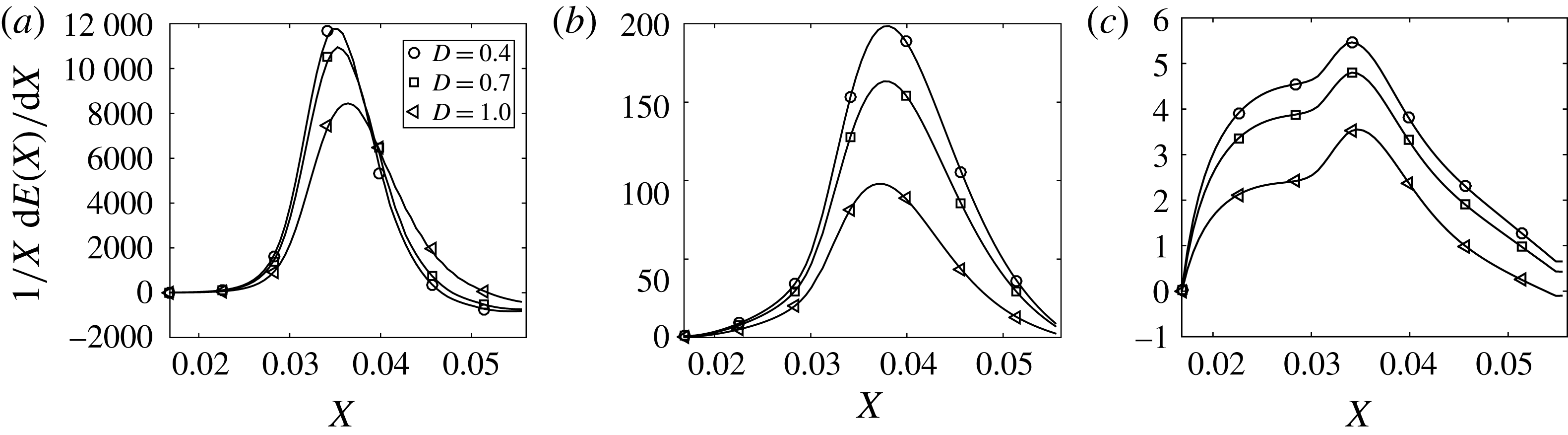
In regard to the variation of the roughness diameter, figure 17 shows that the differences are not as large as the differences noticed in the previous case. As the diameter is increased the growth rates decrease for all cases, which is expected and commensurate with the results corresponding to the variation of spanwise separation (i.e. as the diameter is increased the gap between the roughness elements decreases, as long as the spanwise separation is kept constant). The growth rates corresponding to the control based on wall deformations are almost two orders of magnitude smaller than the growth rates corresponding to the control based on wall transpiration here.

Figure 17.

Growth rate of energy as a function of the streamwise direction: (a) no control; (b) control based on wall transpiration; (c) control based on wall deformation ( $\unicode[STIX]{x1D6EC}^{\ast }=1.2$  cm).

5 Discussion of the physical mechanism behind the control strategies

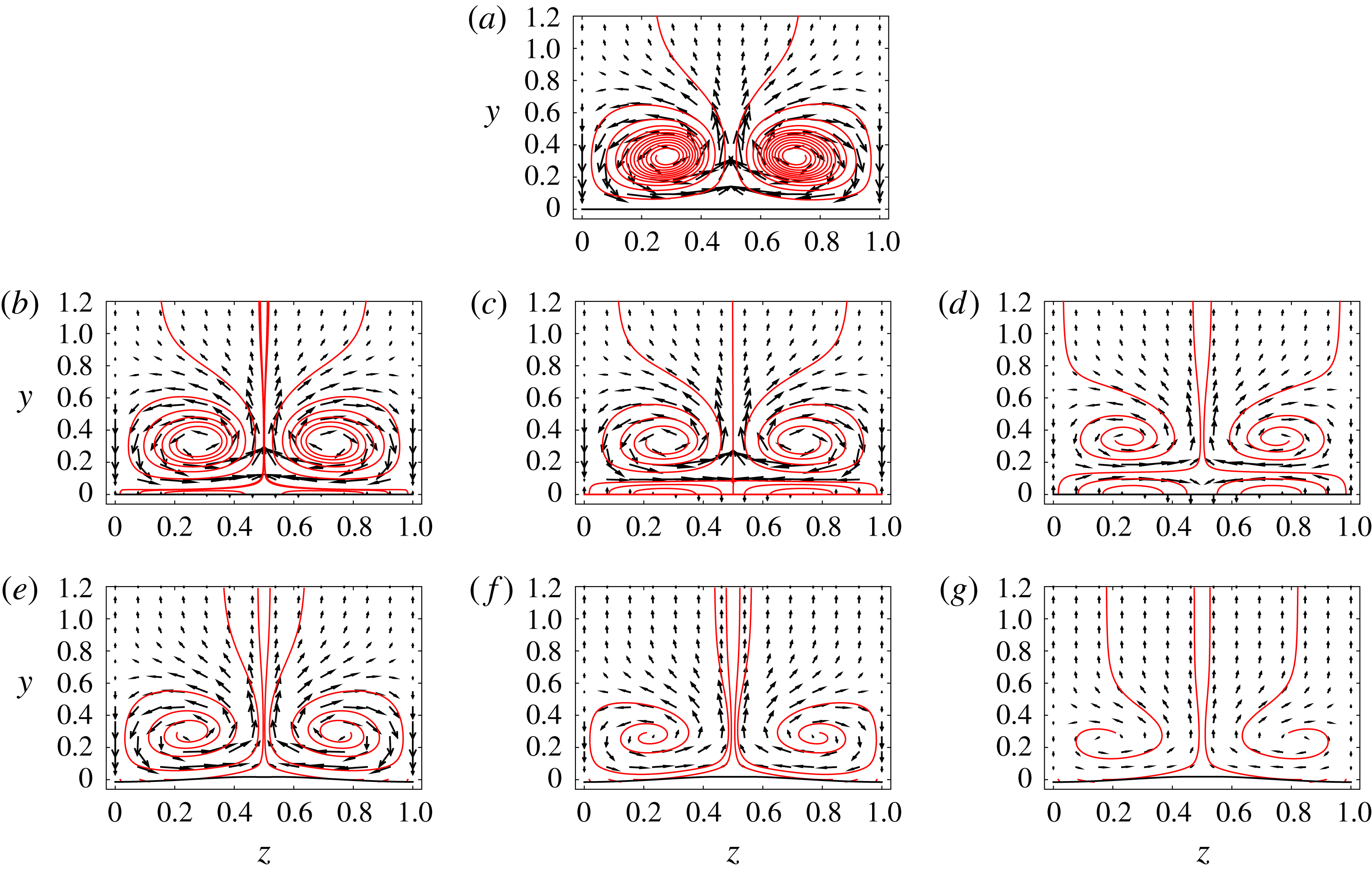
In this section, we discuss the main physical mechanisms that are behind the control based on wall transpiration and wall deformation, and explain why the latter is more effective than the former in reducing the vortex energy. In figure 18, we plot two-dimensional vector fields $(v,w)$ and streamlines in a cross-plane $(y,z)$ located in $X=0.04$ , for the spanwise separation $\unicode[STIX]{x1D6EC}^{\ast }=1.2$  cm. Two streamlines were seeded in close proximity to the centres of two vortices, while other streamlines were seeded from the wall. These latter have meaning for control based on wall transpiration because the velocity is non-zero at the wall as a result of blowing and suction. The top plot (figure 18 a) represents the uncontrolled flow, and it shows two counter-rotating vortices lifting low momentum from the wall at the spanwise location between the two vortices, as well as distributing high momentum fluid from the upper layers to the wall at the $z=0$ or $z=1$ planes. It is well known that this exchange of high and low momentum in the vertical direction brings about variations of the streamwise velocity along the spanwise direction, which is the main driver of high- and low-speed streaks.

Figure 18.

Two-dimensional vector fields $(v,w)$ and streamlines in a cross-plane $(y,z)$ located in $X=0.04$ : (a) uncontrolled flow; (b) wall transpiration control, iteration 1; (c) wall transpiration control, iteration 5; (d) wall transpiration control, iteration 10; (e) wall deformation control, iteration 1; (f) wall deformation control, iteration 5; (g) wall deformation control, iteration 10 ( $\unicode[STIX]{x1D6EC}^{\ast }=1.2$  cm).

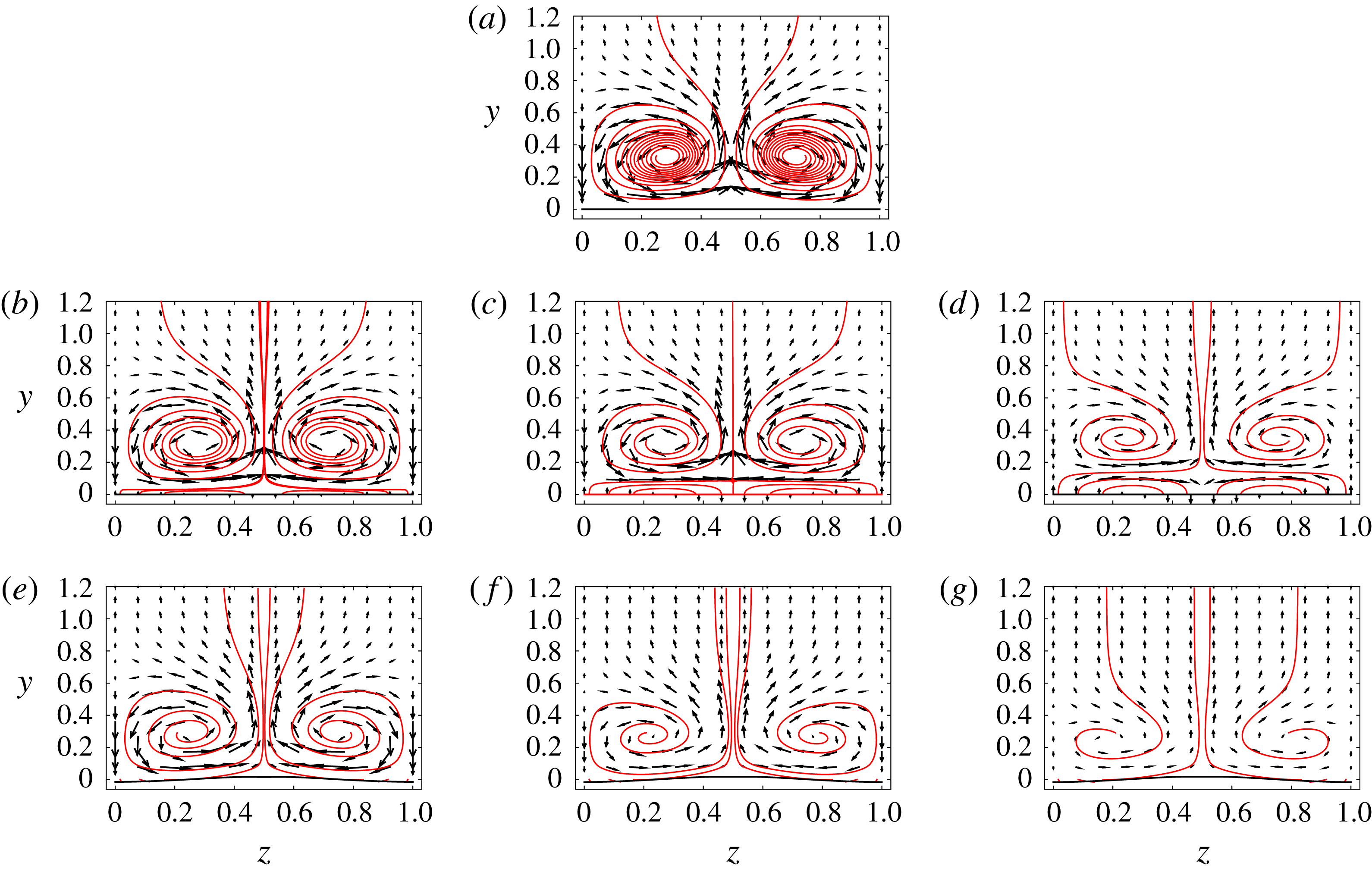
Panels 18(b) and 18(e) represent the vortices for the control based on wall deformation and transpiration, respectively, after the first iteration in the control algorithm. The other panels of the figure (18 c,d,f,g) represent the vortices at two subsequent iterations as indicated in the figure caption. As the number of iterations in the control algorithm increases, a weakening of the vortex strength is apparent as a result of both control algorithms. The strength of the vortex is qualitatively measured here by the length of the arrows of the two-dimensional vector field $(v,w)$ . The ‘relaxation’ of vortices is also revealed by the evolution of the streamline that is seeded from a location that is close to the centre of the vortex. For the uncontrolled flow in figure 18(a), it is noted that these streamlines are very close to each other; as the iteration number increases, however, the streamlines become more scarce and distant from one another (this is more prevalent for the control based on wall deformation). For the control based on wall transpiration in 18(b–d), an additional weak vortical flow is initiated in the vicinity of the wall due to a spanwise alternation of blowing and suction. This forces the two counter-rotating vortices to move upward, changing the vertical location of the Görtler vortex.

Figure 19.

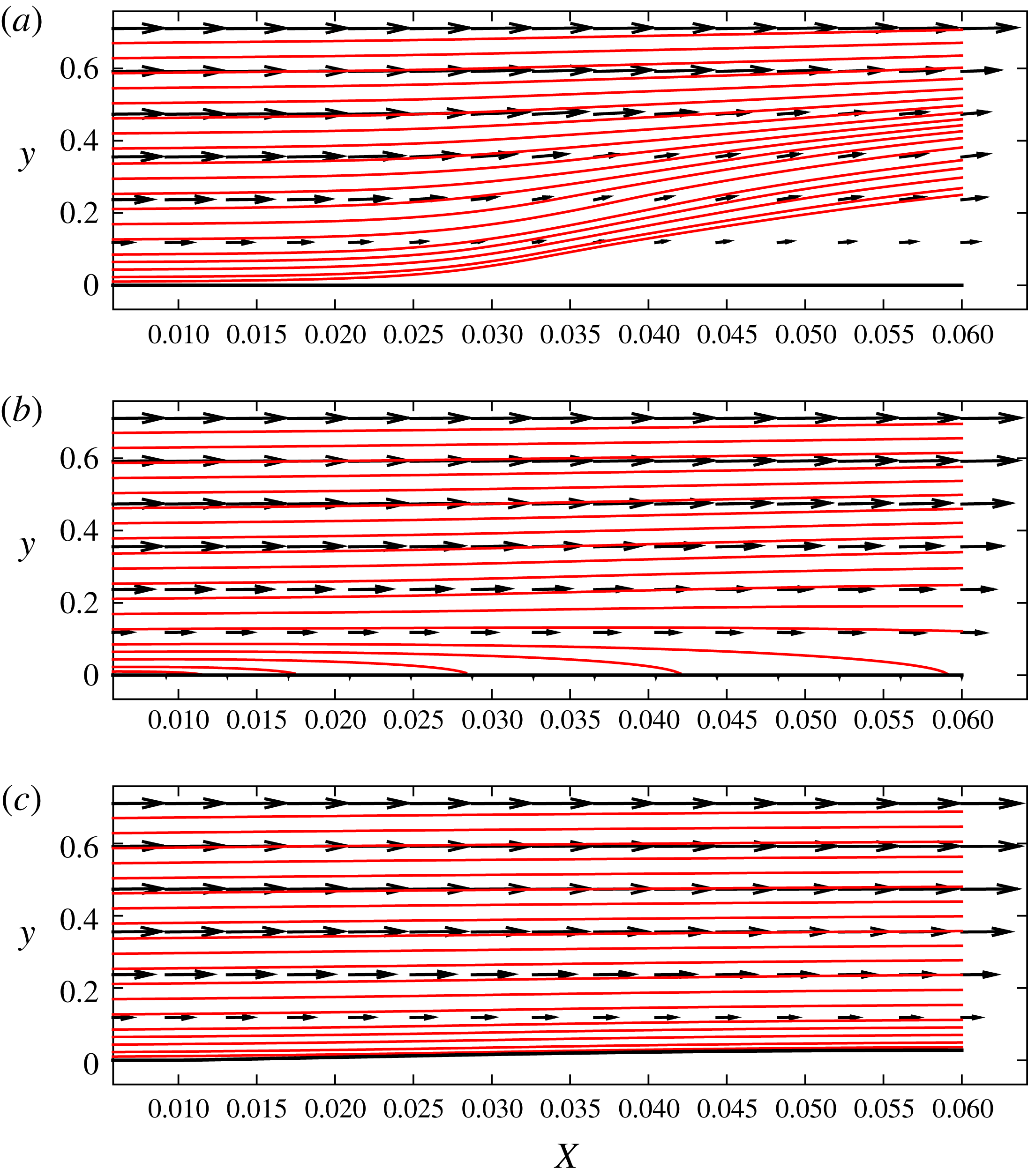
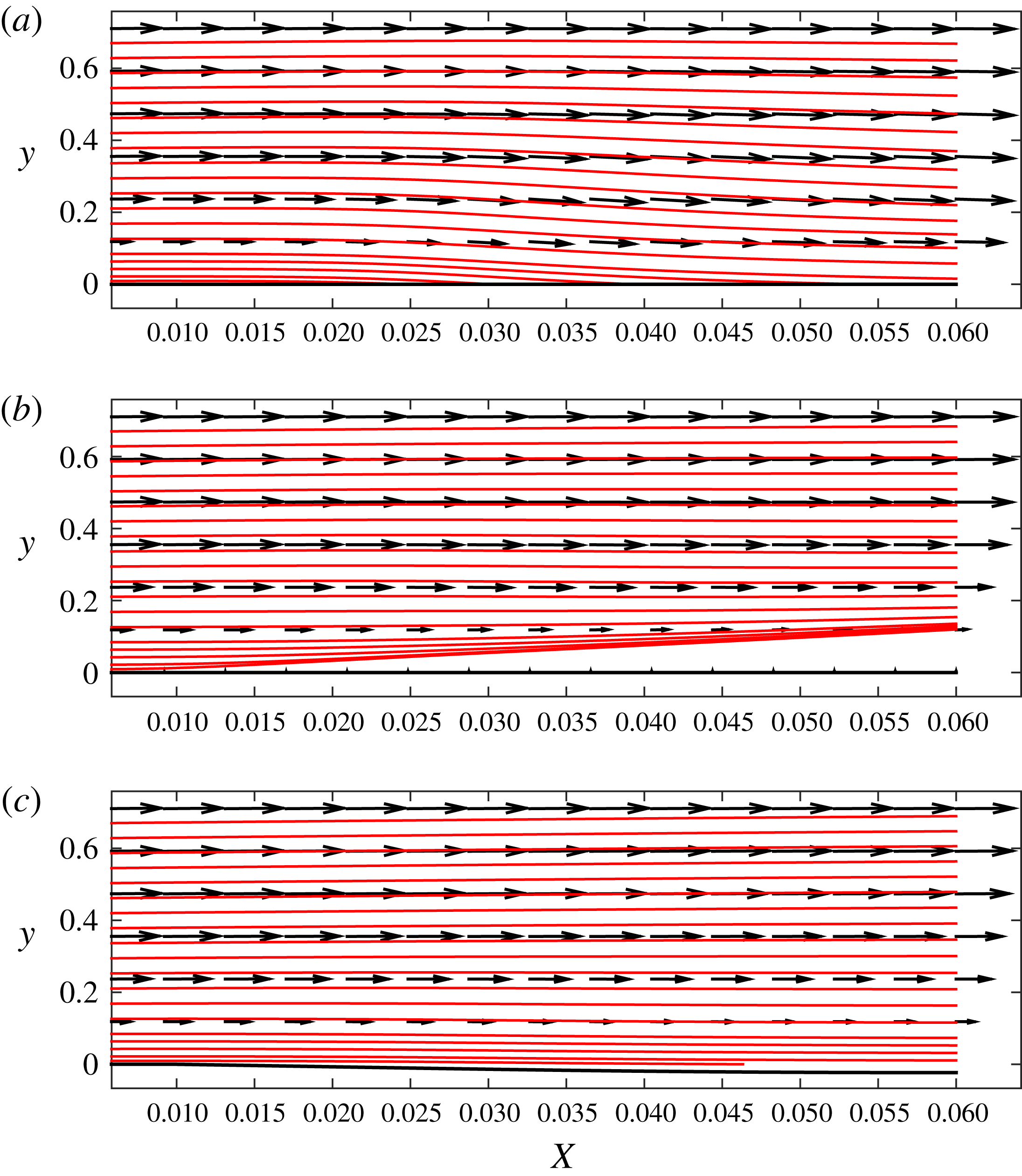
Two-dimensional vector fields $(u,v)$ and streamlines in a sectional plane $(X,y)$ located in $z=0.5$ (where low momentum fluid particles are lifted from the wall): (a) uncontrolled flow; (b) wall transpiration control; (c) wall deformation control ( $\unicode[STIX]{x1D6EC}^{\ast }=1.2$  cm).

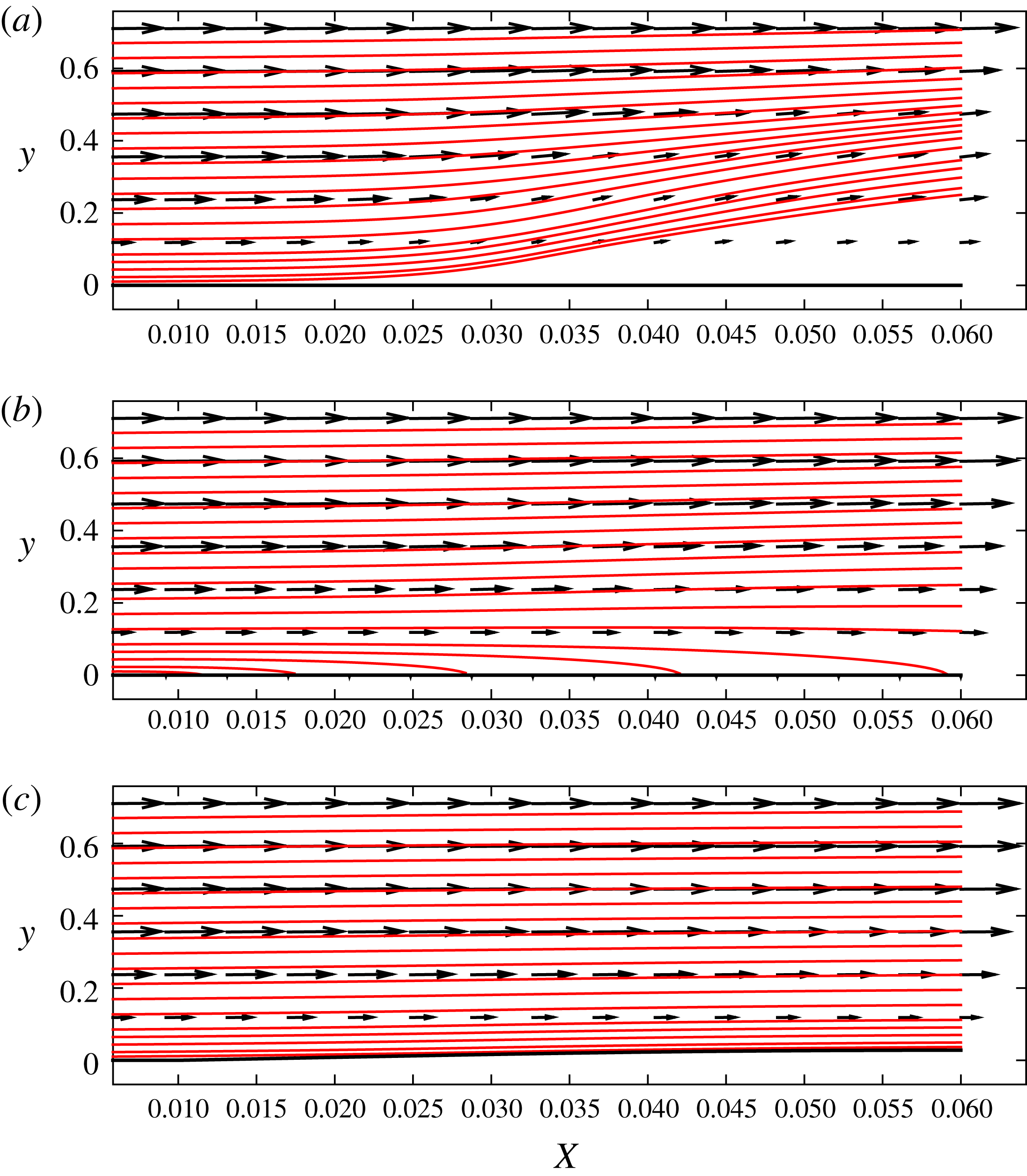
In figures 19 and 20, we plot two-dimensional vector fields and streamlines for uncontrolled and controlled boundary layers, in sectional planes $(x,y)$ that are located at $z=0.5$ and $z=0$ , respectively. In figure 19(a), corresponding to the uncontrolled flow, streamlines that are seeded in close proximity to the wall reveal how fluid particles carrying low momentum are lifted up from the lower layers to the upper layers. The deceleration of fluid particles can be noted by inspecting the variation of the length of arrows that form the vector field (the length of the arrows is proportional to the velocity magnitude in its location): by following the horizontal line of vectors starting from the left boundary at approximately $y=0.36$ in figure 19(a), one can notice how the length of arrows decreases as the fluid particle advances downstream. Now, if one inspects the same line of vectors in 19(b) or 19(c) (initiated at $y=0.36$ from the left), it is seen that the length of the arrow does not change much as the fluid particle moves downstream (there is a very small decrease for control based on wall transpiration in figure 19 b). The streamline at this wall-normal location ( $y=0.36$ ) is also parallel to the wall for both control cases, while the same streamline in the uncontrolled case (figure 19 a) shows a significant deviation in the upward direction. The same conclusions can be reached for the line of vectors located at $y=0.12$ (the streamline associated with this location is parallel to the wall as well). Below this level ( $y=0.12$ ), however, there are differences between the two control algorithms: first, the suction effect is revealed in figure 19(b) by the first five streamlines changing direction and ending at the wall because the fluid particles are absorbed into the wall; second, figure 19(c) shows a slight deviation of the wall line in the upward direction as a results of the control scheme, which accelerates fluid particle, thus increasing the momentum in the vicinity of the wall (all streamlines in this case become parallel to the wall).

Figure 20.

Two-dimensional vector fields $(u,v)$ and streamlines in a sectional plane $(X,y)$ located in $z=0$ (where low momentum fluid particles are brought to the wall): (a) uncontrolled flow; (b) wall transpiration control; (c) wall deformation control ( $\unicode[STIX]{x1D6EC}^{\ast }=1.2$  cm).

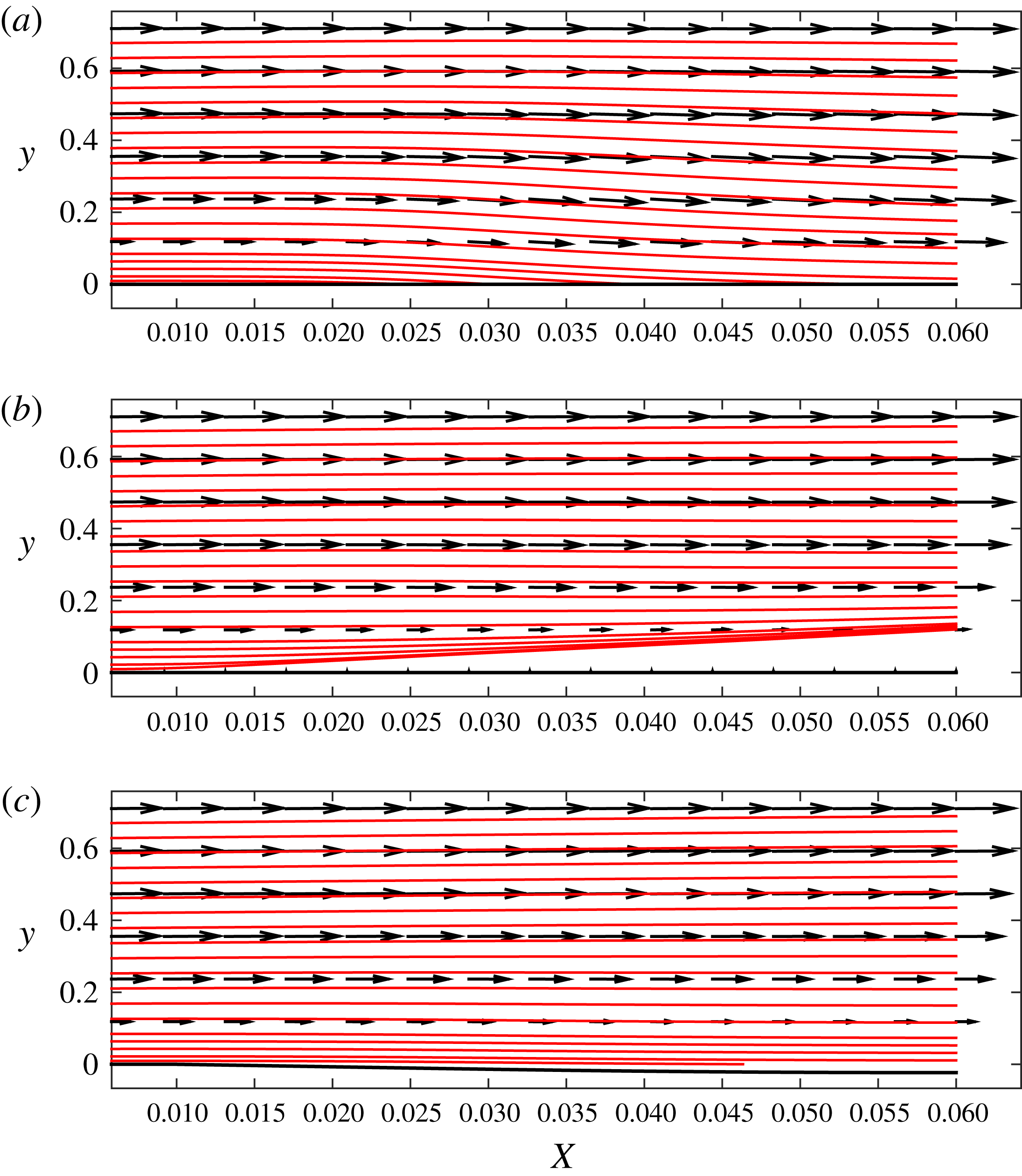
In figure 20, the same picture as in figure 19 is shown, except that another spanwise location corresponding to the downwelling of the fluid particle from the upper layers to the wall is considered. As mentioned before, at this spanwise location $z=0$ high momentum from above is brought downward, which can be clearly noticed by the increase in the length of arrows along the line of vectors that starts at approximately $y=0.12$ or $y=0.25$ from the left boundary. Shown in figure 20(a) are also streamlines that deviate towards the wall as a result of the counter-rotation posed by the vortices. The effect of blowing at this spanwise location is seen in figure 20(b), where the streamlines are deviated from the wall; this brings about changes in the upper layers, where fluid particles are constrained to move at a constant speed and in a trajectory that is parallel to the wall (see the line of vectors that starts at $y=0.25$ , for example). In figure 20(c), the downward deviation of the wall geometry can be seen, which slows down the fluid particles gently, thus decreasing the momentum in the proximity to the wall; again, this yields a constant velocity along the vector lines, with streamlines that remain parallel to the wall.

Finally, in figure 21 we plot two-dimensional vector fields $(u,w)$ and streamlines in two sectional planes $(x,z)$ that are parallel to the wall, one very close to the wall ( $y=0.02$ ) and the other at $y=0.15$ (the reason for choosing the latter becomes clear when looking at vectors and streamline plots in figures 19 and 20; at this elevation the velocity is constant along a horizontal line, and the streamline is parallel to the wall). The uncontrolled flow in figure 21(a), corresponding to the plane $y=0.02$ , shows a deviation of fluid particles towards $z=0.5$ line, which is the effect of counter-rotating vortices; this produces a small cross-flow component. As a result of the control, as shown in figure 21(b,c), the fluid particles are brought back to their original upstream trajectories, with the cross-flow component being negligible (note that a small cross-flow component is still seen in the plot corresponding to the control based on wall transpiration). At the other elevation ( $y=0.15$ ), there is somewhat smaller cross-flow component in the uncontrolled case (figure 21 d) as expected, and no cross-flow component for both control cases.

Figure 21.

Two-dimensional vector fields $(u,w)$ and streamlines in a sectional plane $(X,z)$ parallel to the wall: (a) uncontrolled flow, $y=0.02$ ; (b) wall transpiration control, $y=0.02$ ; (c) wall deformation control, $y=0.02$ ; (d) uncontrolled flow, $y=0.15$ ; (e) wall transpiration control, $y=0.15$ ; (d) wall deformation control, $y=0.15$ ( $\unicode[STIX]{x1D6EC}^{\ast }=1.2$  cm).

Different mechanisms towards controlling a boundary layer flow distorted by centrifugal instabilities are at play here for the two schemes introduced in this study:

1. (i) For control based on wall deformation, a positive displacement of the wall (at the spanwise location between the two vortices, as seen in figure 19 c) accelerates fluid particles in the streamwise direction, while negative displacement (see figure 20 c) decelerates them. This means that the momentum of fluid particles in close proximity to the wall (in between the vortices) is increased, thus weakening the effect of lift up of low momentum fluid particles from the wall, as previously described. The opposite occurs at negative displacement locations, where the momentum of fluid particles at the wall is decreased. There is also an effect (although small) on the cross-flow velocity component as shown in figure 21.

2. (ii) The mechanism behind the control based on wall transpiration closely resembles the opposition control type, as introduced and described in previous studies concerning turbulent boundary layers or channel flows (see, for example, Choi et al. Reference Choi, Moin and Kim1994, Koumoutsakos Reference Koumoutsakos1997, Reference Koumoutsakos1999, Stroh et al. Reference Stroh, Frohnapfel, Schlatter and Hasegawa2015), although, here, the sensor is not the vertical velocity measured in a plane parallel to the wall. However, as seen in figure 18(b,d,f), blowing is applied in regions where the vertical velocity in the flow is negative, and suction is applied where the vertical velocity in the flow is positive; this is the main mechanism of reducing the energy of the Görtler vortices. Compared to the control based on wall deformation, the effect on the cross-flow velocity is more significant as shown in figure 18(f), where the vortical flow induced by alternating blowing and suction contributes to the increase of the cross-flow.

We emphasize again that there are significant differences between the steady Görtler vortices considered here and the wall turbulence considered in previous studies that might explain why, for wall turbulence, it was found that the control based on wall transpiration can be more effective than wall deformation. As mentioned previously, we solve a parabolic problem in steady state, where we assume variations in the streamwise direction to be small for both the flow and wall geometry. One of the reasons that the wall deformation control is more effective than the wall transpiration control, in our study, is clear from the previous discussions of vector fields and streamlines (figures 18–21): in a nutshell, the alternation of blowing and suction in the spanwise direction for the former type of control introduces an additional vortical flow that, on one hand, deviates or attracts streamlines from/to the wall, and, on the other hand, influences the cross-flow in proximity to the wall; this is not the case for the control based on wall deformation, where it was found that the mechanism of flow alteration is different. Moreover, in the control based on wall transpiration case, the additional vortical flow induced in the vicinity of the wall forces Görtler vortices to move slightly upward, thus preventing their complete elimination.

6 Summary and conclusions

An optimal control strategy in the high Reynolds number asymptotic framework was derived and tested on Görtler vortices developing along a concave surface. The Navier–Stokes equations were simplified to obtained the boundary region equations (BRE), which are a parabolic set of equations since the streamwise pressure derivative and the second derivative were neglected. The effect of wall deformations was incorporated into the model by a Prandtl transformation applied to the BRE, which was then solved numerically using a marching algorithm. The variations in local surface shape then allowed for a relatively straightforward control strategy to be implemented to the transformed set of equations in order to determine the optimum wall deformation or transpiration that reduced the energy of the vortices. Görtler vortices were initiated by perturbing the upstream flow with a periodic array of roughness elements placed near the leading edge, using a previously derived asymptotic solution to obtain the upstream boundary conditions (Goldstein et al. Reference Goldstein, Sescu, Duck and Choudhari2010, Reference Goldstein, Sescu, Duck and Choudhari2011). The vortex energy was controlled via an optimal control algorithm based on Lagrange multipliers and adjoint equations, where the wall displacement or the wall transpiration velocity serves as the control variable. The modified BREs equations (2.9)–(2.12) explicitly included an arbitrary function ${\mathcal{F}}(X,z)$ representing the local surface deformation, and therefore provided a parametric mechanism for the optimal control. The optimal control strategy was aimed at minimizing the difference between the calculated wall shear stress and the Blasius shear stress. The cost functional was defined in terms of the energy associated with the Görtler vortices, and the sensors were functions of the wall shear stress. Local wall deformations appeared to resemble elongated surface shapes, in the form of streaks, that we optimized to control the Görtler vortex energy.

An extensive numerical study of the effect of controlled wall deformation versus transpiration on the vortex development for incompressible boundary layer flow over a curved wall has been performed. Various results in terms of contour plots of streamwise velocity, energy distribution in the streamwise direction or distributions of the spanwise average shear stress showed that the optimal control algorithm is very effective in counteracting the Görtler vortices. The kinetic energy associated with the vortices was shown to decrease by almost three orders of magnitude from the original amplitude in some cases, with a commensurate reduction in the wall shear stress. Our results clearly indicate that the controlled surface deformations are more effective than wall transpiration in altering the streamwise development of the Görtler vortices for a given roughness height and spanwise wavelength. Potential explanations for this difference were given, and the physical mechanism behind the control was described. It was found that for control based on wall deformation, a positive displacement of the wall accelerates fluid particles in the streamwise direction, while negative displacement decelerates them, which means that the fluid momentum at the wall is increased, weakening the ‘lift-up’ effect. The opposite was shown to occur at negative displacement locations, where the momentum of fluid particles at the wall is decreased. On the other hand, for control based on wall transpiration, blowing is applied in regions where the vertical velocity in the flow is negative, and suction is applied where the vertical velocity in the flow is positive (this is similar to the ‘opposition control’ mechanism that was introduced in the framework of control of turbulent channel flows (Choi et al. Reference Choi, Moin and Kim1994)) which is the main mechanism behind the reduction of the energy of the Görtler vortices. The fact that wall-deformation-based control was found to be more effective than wall transpiration in our formulation of the control problem is clear in the discussion and pictorial representation of velocity field and streamlines of both types of control mechanisms (see figures 18–21).

While the boundary layer was excited by a row of roughness elements as derived in Goldstein et al. (Reference Goldstein, Sescu, Duck and Choudhari2010), the algorithm can be easily extended to include free-stream disturbances or turbulence at the upstream boundary. The proposed control algorithm has potential application to a number of realistic problems including aircraft wing design, to mitigate induced drag, or in supersonic wind tunnels, where it is known that flow instabilities in the test section are triggered by Görtler vortices developing on the concave portion of the walls. Of course, the latter application will necessitate the extension of the algorithm into the compressible regime, which is a matter of future analysis.