Introduction to logpar ‘finite lifetime’ curves

If our reader would like to read just the first three pages (pages 41–42–43) of our OPEN ACCESS published paper https://multimediafluids.uam.elogim.com/core/journals/international-journal-of-astrobiology/article/div-classtitlenew-evo-seti-results-about-civilizations-and-molecular-clockdiv/494A1FECFF9A5A08E91662A8D57573DE then he/she would immediately realize why we were forced to introduce the notion of FINITE LIFETIME as the new logpar curve.

The idea is easy: we seek to represent any lifetime by virtue of just three points in time: birth, peak, death (b, p, d). No other point in between. That is, no other ‘senility point’ s such as those appearing in all b-lognormals that this author had published in his Evo-SETI Theory prior to 2017 (Maccone, Reference Maccone2010, Reference Maccone2011, Reference Maccone2012, Reference Maccone2013, Reference Maccone2014, Reference Maccone2015). In fact, it is easier and more natural to describe someone's lifetime just in terms of birth, peak and death, than in terms of birth, senility and death, because when the senility arrives is rather uncertain. In other words, it is so hard to define in the practice for any individual when his/hers senility occurs.

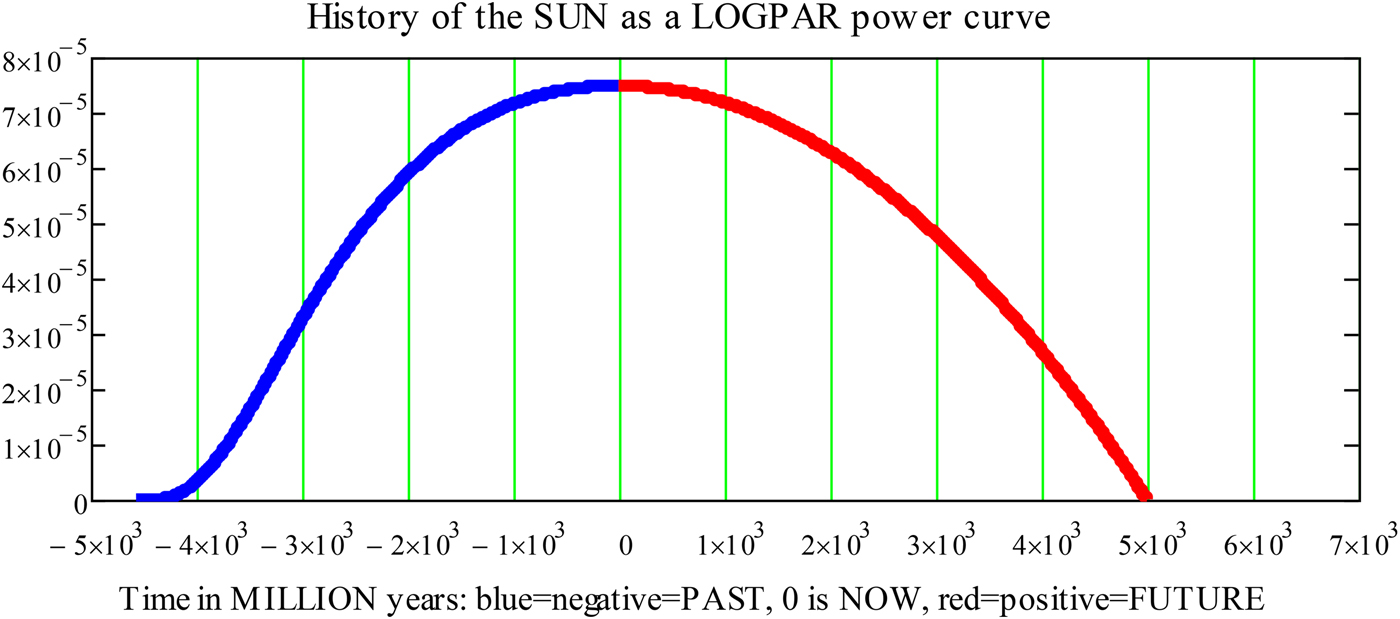
In the first part of Fig. 1, the curve shown in blue on the left, i.e. prior to the peak time p, has just the same shape as a b-lognormal: it starts at birth time b, climbs up to the adolescence time a (ascending inflexion point of the b-lognormal) (in reality the adolescence time should more properly be called ‘puberty time’ since it marks the beginning of the reproduction capacity for that individual) and finally reaches the peak time at p (the maximum, i.e. the point of zero first derivative of the b-lognormal). All this is just ordinary b-lognormal stuff, as we have been ‘preaching’ since about 2012, except that our present b-lognormal does not fulfill the normalization constant and so it is not a probability density anymore.

Fig. 1.

History of the Sun as a logpar power curve, created only by assigning the three numeric input logpar values (b = −4.567 · 10⁹ year, p = 0, year, d = 5 · 10⁹ year). The Sun formed about 4.6 billion years ago from the collapse of part of a giant molecular cloud that consisted mostly of hydrogen and helium and that probably gave birth to many other stars. This age is estimated using computer models of stellar evolution and through nucleocosmochronology. The result is consistent with the radiometric date of the oldest Solar System material, at 4.567 billion years ago (see the Wikipedia site https://en.wikipedia.org/wiki/Sun#Formation). The Sun is now producing energy at about a constant rate and it will keep doing so for at least a billion year in the future. The above graph reveals so since in the next billion year the energy production of the Sun will change by less that 10⁻¹¹ (a femto). In the above graph the b-lognormal power curve (not a probability density any more, since not normalized to 1 any more) is covering the time between the birth of the Sun 4.567 billion years ago and nowadays and is shown in blue. On the contraty, the logpar part between now and 5 billion years in the future is shown in red and is just a parabola with its vertex at the peak of the b-lognormal. This author is not claiming that the above logpar curve is the Sun's actual evolution curve in any astrophysical sense: it is just a good visual logpar example.

But now the real novelty comes, i.e. the second part of the curve, the one on the right, shown in red. That is just a parabola having its vertex exactly at the peak time p. Notice that this definition automatically implies that the tangent line at the peak is horizontal, i.e. the same for both the b-lognormal and the parabola. Notice also that, after the peak, the parabola plunges down until it reaches the time axis at the death time d. Therefore this new definition of death time d is different from the old definition of d applying to b-lognormals plus a descending straight line with a junction at the senility point s (descending inflexion point of the b-lognormal), as we did prior to 2017.

And this is the LOGPAR (b-LOGnormal plus PARabola) new CURVE FINITE IN TIME (namely ranging in time just between birth and death). In the present paper we study the logpar curve with surprising results bringing in the extremely important physical notion of ENERGY.

Finding the parabola equation of the right part of the logpar

We shall now cast into appropriate mathematics the above popular description of what a logpar curve is.

Consider the equation of a parabola in the time t having its vertical axis along the t = p vertical line:

(1)$$y = \alpha \;(t - p)^2 + \beta \;(t - p) + \gamma, $$

where α, β and γ are the three coefficients of the time that we must determine according to the assumptions shown in Fig. 1. To find them, we must resort to the three conditions that we know to hold by virtue of a glance to Fig. 1:

1. (1) #1 CONDITION: the height of the peak is P, just the same as the height of the peak of the b-lognormal on the left in Fig. 1. Thus, inserting the two equations of the peak, namely

   (2)$$\left\{ {\matrix{ {t = p} \cr {y = P} \cr}} \right.$$
   into (1), the latter yields immediately
   (3)$$P = \gamma $$
   that, when inserted back into (1), changes it into
   (4)$$y = \alpha \;(t - p)^2 + \beta \;(t - p) + P.$$

2. (2) #2 CONDITION: the tangent straight line at both the b-lognormal and the parabola at the peak abscissa p is horizontal. In other words, the first derivative of (4) at t = p must equal zero. Differentiating (4) with respect to t, equalling that to zero and then solving for β yields

   (5)$$\beta = - \,2\,\alpha \,(t - p).$$
   Inserting (5) into (4), the latter is turned into
   (6)$$y = - \;\alpha \;(t - p)^2 + P.$$

3. (3) #3 CONDITION: at the death time d, one must have y = 0, yielding from (6) the equation

   (7)$$0 = - \;\alpha \;\left( {d - p} \right)^2 + P.$$

Solving (7) for α one gets

(8)$$\alpha = \displaystyle{P \over {{\left( {d - p} \right)}^2}}.$$

Finally, inserting (8) into (6) the desired equation of the parabola is found

(9)$$y(t) = P\left[ {1 - \displaystyle{{{\left( {t - p} \right)}^2} \over {{\left( {d - p} \right)}^2}}} \right].$$

As confirmation, one may check that (9) immediately yields the two conditions

(10)$$\left\{ {\matrix{ {y(\,p) = P} \cr {y(d) = 0\,.} \cr}} \right.$$

Finding the b-lognormal equation of the left part of the logpar

As for the b-lognormal between birth and peak, making up the left part of the logpar curve, we already know all its mathematical details from the previous many papers published by this author on this topics, but we shall summarize here the main equations for the sake of completeness.

The equation of the b-lognormal starting at b reads

(11)$${\rm b\_lognormal}(t;\mu, \sigma, b) = \displaystyle{{{\rm e}^{ - ({({\rm ln} (t - b) - \mu )}^2/2\sigma ^2)}} \over {\sqrt {2\pi} \,\sigma \,(t - b)}}.$$

Tables listing the main equations that can be derived from (11) were given by this author in refs. [Maccone Reference Maccone2012] and [Maccone Reference Maccone2013] and we shall not re-derive them here again. We just confine ourselves to reminding that:

1. (1) The abscissa p of the peak of (11) is given by

   (12)$$p = b + {\rm e}^{\mu - \sigma ^2}.$$

Proof. Take the derivative of (11) with respect to t and set it equal to zero. Then solve the resulting equation for t, that now becomes p and (12) is found.

1. (2) The ordinate p of the peak of (11) is given by

   (13)$$P = \displaystyle{{e^{\textstyle{{\sigma ^2} \over 2} \scriptstyle{- \mu }}} \over {\sqrt {2 \pi }\sigma }}$$

Proof. Rewrite p instead of t in (11) and then insert (12) instead of p. Then simplify to get (13).

1. (3) The abscissa of the adolescence point (that should actually be better named ‘puberty point’) is the abscissa of the ascending inflexion point of (11). It is given by

   (14)$$a = b + e^{ - \textstyle{{\sigma \sqrt {\sigma ^2 + 4} } \over 2} - \textstyle{{3\sigma ^2} \over 2} \scriptstyle{+ \mu} }$$

Proof. Take the second derivative of (11) with respect to t and set it equal to zero. Then solve the resulting equation for t, that now becomes a and (14) is found.

1. (4) The ordinate of the adolescence point is given by

   (15)$$\displaystyle{{{\rm e}^{ - (\sigma \sqrt {\sigma ^2 + 4} /4) + (\sigma ^2/4) - \mu - (1/2)}} \over {\sqrt {2\pi} \sigma}}. $$

Proof. Just rewrite a instead of t in (11) and then insert (14) and simplify the result.

Let us now notice that, within the framework of the logpar theory described in this paper, we may NOT say that (11) fulfills the normalization condition

(16)$$\int_b^\infty {{\rm b\_lognormal}(t;\mu, \sigma, b)} dt = 1\;,$$

since (11) here is only allowed to range between b and p. Rather than adopting (16), we must thus replace (16) by the integral of (11) between b and p only. Fortunately, it is possible to evaluate this integral in terms of the error function defined by

(17)$${\rm erf}(x) = \displaystyle{2 \over {\sqrt \pi}} \int_0^x {{\rm e}^{ - t^2}dt}. $$

In fact, the integral of the b-lognormal (11) between b and p turns out to be given by

$$\eqalign{& \int_b^p {{\rm b\_lognormal}(t;\mu, \sigma, b)} dt = \cr & \quad= \int_b^p {\displaystyle{{{\rm e}^{ - \;({\left( {{\rm ln} (t - b) - \mu} \right)}^2/2\sigma ^2)}} \over {\sqrt {2\pi} \,\sigma \,\left( {t - b} \right)}}dt} \cr & \quad= \displaystyle{{1 + {\rm erf}\left( {\sqrt 2 \ln \left( {\,p - b} \right) - \sqrt 2 \,\mu /2\,\sigma } \right)} \over 2} =} $$

Now, inserting (12) instead of p into the last erf argument, a remarkable simplification occurs: μ and b both disappear and only σ is left. In addition, the erf property erf( − x) = −erf(x) allows us to rewrite

(18)$$= \displaystyle{{1 + {\rm erf}\left( { - \sigma /\sqrt 2 } \right)} \over 2} = \displaystyle{{1 - {\rm erf}\left( {\sigma /\sqrt 2 } \right)} \over 2}.$$

In conclusion, the area under the b-lognormal between birth and peak is given by

(19)$$\int_b^p {{\rm b\_lognormal}(t;\mu, \sigma, b)} dt = \displaystyle{{1 - {\rm erf}\left( {\sigma /\sqrt 2 } \right)} \over 2}\,.$$

This result will prove to be of key importance for the further developments described in the present paper.

Area under the parabola on the right part of the logpar between peak and death

We already proved that the parabola on the right part of the logpar curve has equation (9). Now we want to find the area under this parabola between peak and death, that is

(20)$$\eqalign{& \int_p^d {\left\{ {P\left[ {1 - \displaystyle{{{\left( {t - p} \right)}^2} \over {{\left( {d - p} \right)}^2}}} \right]} \right\}} \;dt = \cr & \quad \quad = P\left( {d - p} \right) - \displaystyle{P \over {{\left( {d - p} \right)}^2}}\int\limits_p^d {{\left( {t - p} \right)}^2} \;dt = \cr & \quad \quad = P\left( {d - p} \right) - \displaystyle{P \over {{\left( {d - p} \right)}^2}}\displaystyle{{{\left( {d - p} \right)}^3} \over 3} = \cr & \quad \quad = \displaystyle{{2\,P\left( {d - p} \right)} \over 3} = \cr & \quad \quad = \displaystyle{1 \over 2} \cdot \left[ {\displaystyle{4 \over 3}P\left( {d - p} \right)} \right] = \displaystyle{1 \over 2} \cdot \left[ {\matrix{ {{\rm Area}\;{\rm of}\;{\rm Archimedes}} \cr {{\rm parabolic}\;{\rm segment,}} \cr {{\rm proved}\;{\rm \lt 212}\;{\rm B}{\rm. C}{\rm.}} \cr}} \right].} $$

The great Ancient Greek mathematician Archimedes (circa 287 B.C.–212 B.C.) of Syracuse (Sicily) already ‘knew’ the last integral result even before the Calculus was discovered by Newton and Leibniz after 1660. More appropriately, (20) is a special case of Cavalieri's quadrature formula (1635, https://en.wikipedia.org/wiki/Cavalieri%27s_quadrature_formula). Actually, Archimedes used the ‘method of exhaustion’ to compute the area of a segment of the parabola, as very neatly described at the site https://en.wikipedia.org/wiki/The_Quadrature_of_the_Parabola.

In conclusion, the area under our parabola between peak and death is given by (20), that we now rewrite as

(21)$$\int_p^d {\left\{ {P\left[ {1 - \displaystyle{{{(t - p)}^2} \over {{(d - p)}^2}}} \right]} \right\}} \;dt = \displaystyle{{2\,P(d - p)} \over 3}.$$

Area under the full logpar curve between birth and death

We are now in a position to compute the full area A under the logpar curve, that is given by the sum of equations (19) and (21), that is

(22)$$\displaystyle{{1 - {\rm erf}\left( {\displaystyle{\sigma \over {\sqrt 2}}} \right)} \over 2} + \displaystyle{{2\,P(d - p)} \over 3} = A.$$

This is really an important equation for this paper.

In fact, if we want the logpar to be a truly probability density function (pdf), we must assume in (22)

(23)$$A = 1.$$

But, surprisingly, we shall NOT do so!

Let us rather ponder over what we are doing:

1. (1) We are creating a ‘Mathematical History’ model where the ‘unfolding History’ of each Civilization in the time is represented by a logpar curve.

2. (2) The knowledge of only three points in time is requested in this model: b, p and d.

3. (3) But the area under the whole curve depends on σ as well as on μ, as we see upon inserting (13) instead of P into (22), that is

   (24)$$\displaystyle{{1 - {\rm erf}\left( {\sigma /\sqrt 2 \,} \right)} \over 2} + \displaystyle{{{\rm e}^{(\sigma ^2/2) - \mu}} \over {\sqrt {2\pi} \,\sigma}} \cdot \displaystyle{{2\,(d - p)} \over 3} = A(\mu, \sigma ).$$

4. (4) Also p is to be replaced by its expression (12) in terms of σ and μ, yielding the new equation

   (25)$$\displaystyle{{1 - {\rm erf}\left( {\sigma /\sqrt 2 \,} \right)} \over 2} + \displaystyle{{{\rm e}^{(\sigma ^2/2) - \mu}} \over {\sqrt {2\pi} \,\sigma}} \cdot \displaystyle{{2\,\left( {d - b - {\rm e}^{\mu - \sigma ^2}} \right)} \over 3} = A(\mu, \sigma ).$$

5. (5) The meaning of (25) is that birth and death are fixed, but the position of the peak may move according to the different numeric values of σ and μ.

6. (6) In addition to that, we ‘dislike’ the presence of the error function erfin (25) since this is not an ‘ordinary’ function, i.e. it is one of the functions that mathematicians call ‘higher transcendental functions’, having complicated formulae describing them. Thus, we would rather get rid of erf.

How may we do so?

The area under the logpar curve depends on sigma only, and here is the area derivative with respect to sigma

The simple answer to the last question (6) is ‘by differentiating both sides of (25) with respect to σ’. In fact, the derivative of the erf function (17) is just the ‘Gaussian’ exponential

(26)$$\displaystyle{{d\,{\rm erf}(x)} \over {dx}} = \displaystyle{2 \over {\sqrt \pi}} \cdot {\rm e}^{ - x^2},$$

and so the erf function itself will disappear by differentiating (25) with respect to σ. In fact, the derivative of the first term on the left hand side of (25) simply is, according to (26),

(27)$$\displaystyle{d \over {d\sigma}} \left[ {\displaystyle{{1 - {\rm erf}\left( {\sigma /\sqrt 2 \,} \right)} \over 2}} \right] = - \,\displaystyle{{{\rm e}^{ - \;(\sigma ^2/2)}} \over {\sqrt {2\pi}}}. $$

As for the derivative with respect to σ of the second term on the left hand side of (25) we firstly notice that σ appears three times within that term. Thus, the relevant derivative is the sum of three terms, each of which includes the derivative of one of the three terms multiplied by the other two terms unchanged. In equations, one has:

(28)$$\eqalign{& \displaystyle{d \over {d\sigma}} \left[ {\displaystyle{{1 - {\rm erf}\left( {\sigma /\sqrt 2 \,} \right)} \over 2} + \displaystyle{{{\rm e}^{(\sigma ^2/2) - \mu}} \over {\sqrt {2\pi} \,\sigma}} \cdot \displaystyle{{2\,\left( {d - b - {\rm e}^{\mu - \sigma ^2}} \right)} \over 3}} \right] = \cr & \quad \quad = \displaystyle{{2^{(3/2)}{\rm e}^{ - (\sigma ^2/2)}} \over {3\sqrt \pi}} - \displaystyle{{{\rm e}^{ - (\sigma ^2/2)}} \over {\sqrt {2\pi}}} - \displaystyle{{\sqrt 2 \left( { - \;{\rm e}^{\mu - \sigma ^2} + d - b} \right){\rm e}^{\textstyle{{\sigma ^2} \over 2} - \mu}} \over {3\sqrt \pi \sigma ^2}} + \cr & \;\;\quad \quad + \displaystyle{{\sqrt 2 \left( { - \;{\rm e}^{\mu - \sigma ^2} + d - b} \right){\rm e}^{\textstyle{{\sigma ^2} \over 2} - \mu}} \over {3\sqrt \pi}}.} $$

Several alternative forms of this equation (28) are possible and that is rather confusing. However, using a symbolic manipulator (this author did do by virtue of Maxima), a few steps lead to the following form of (28):

(29)$$\eqalign{& \displaystyle{{dA\left( {\mu \left( \sigma \right),\sigma} \right)} \over {d\sigma}} \equiv \displaystyle{{dA\left( \sigma \right)} \over {d\sigma}} = \cr & = - \displaystyle{{\sqrt 2 \left( {d - p} \right){\rm e}^{ - (\sigma ^2/2)}} \over {3\sqrt \pi \left( {\,p - b} \right)\sigma ^2}} + \displaystyle{{\sqrt 2 \left( {d - p} \right){\rm e}^{ - (\sigma ^2/2)}} \over {3\sqrt \pi \left( {\,p - b} \right)}} + \displaystyle{{2^{(3/2)}{\rm e}^{ - (\sigma ^2/2)}} \over {3\sqrt \pi}} \cr & \quad- \displaystyle{{{\rm e}^{ - (\sigma ^2/2)}} \over {\sqrt {2\pi}}} = \cr & = \displaystyle{{\left( {\,p\,\sigma ^2 - 2\,d\,\sigma ^2 + b\,\sigma ^2 - 2p + 2\,d} \right){\rm e}^{ - (\sigma ^2/2)}} \over {3\sqrt {2\pi} \left( {\,p - b} \right)\sigma ^2}}.} $$

This (29) is the derivative of the area with respect to sigma.

Exact ‘history equations’ for each logpar curve

We now take a further, crucial step in our analysis of the logpar curve: we IMPOSE that the derivative of the area with respect to sigma, i.e. (29), is zero

(30)$$\displaystyle{{dA\left( \sigma \right)} \over {d\sigma}} = 0.$$

What does that mean?

Well, hold your breath: (30) is the Evo-SETI LEAST ENERGY PRINCIPLE, i.e. the Evo-SETI equivalent of the LEAST ACTION PRINCIPLE in physics ! This shocking conclusion does not show up at the moment, but it will, at the end of this paper.

For the time being with content ourselves with the ‘crude mathematics’ of rewriting the imposed condition (30) by virtue of the last expression in (29) that, getting rid of both the exponential and the denominator, immediately boils down to

(31)$$p\,\sigma ^2 - 2\,d\,\sigma ^2 + b\,\sigma ^2 - 2p + 2\,d = 0.$$

This is just the quadratic equation in σ

(32)$$\sigma ^2\left( {\,p - 2d + b} \right) = 2\left( {\,p - d} \right),$$

and so we finally get

(33)$$\sigma ^2 = \displaystyle{{2\left( {d - p} \right)} \over {2d - \left( {b + p} \right)}}.$$

This is the most important new result discovered in the present paper. It is the LOGPAR HISTORY EQUATION FOR σ

(34)$$\sigma = \displaystyle{{\sqrt 2 \sqrt {d - p}} \over {\sqrt {2d - \left( {b + p} \right)}}}. $$

In other words, given the input triplet (b,  p,  d) then (33) immediately yields the exact σ ² of the b-lognormal left part of the logpar curve. It was discovered by this author on 22 November 2015 and led not only to this paper, but to the introduction of the ENERGY spent in a lifetime by a living creature, or by a whole civilization whose ‘power-vs-time’ behaviour is given by the logpar curve, as we will understand better in the coming sections of this paper.

At the moment, for reasons that will become obvious later, we confine ourselves to taking the limit of both sides of (34) for d → ∞, with the result

(35)$$\mathop {\lim} \limits_{d \to \infty} \sigma = \mathop {\lim} \limits_{d \to \infty} \displaystyle{{\sqrt 2 \sqrt {d - p}} \over {\sqrt {2d - \left( {b + p} \right)}}} = \mathop {\lim} \limits_{d \to \infty} \displaystyle{{\sqrt 2 \sqrt d} \over {\sqrt {2d}}} = 1.$$

Since we already know that σ must be positive, (35) really shows that σ may range between zero and one only

(36)$$0 \le \sigma \le 1.$$

Next to (34) one of course has a similar LOGPAR EQUATION FOR μ, that is immediately derived from (12) and (34). To this end, just take the log of (12) to get

(37)$$\mu = \ln \left( {\,p - b} \right) + \sigma ^2$$

that, invoking (33), yields the desired logpar equation for μ

(38)$$\mu = \ln (\,p - b) + \displaystyle{{2(d - p)} \over {2d - (b + p)}}.$$

Having proved both (34) and (38), we still have to make an important remark about them. We will put the suffix ‘LH’ (standing for ‘Logpar History’) to each of them to remind their users that they were derived under the assumption (30) that the derivative of the area under the logpar curve is ZERO, amounting to the LEAST ENERGY PRINCIPLE for Evo-SETI Theory. In conclusion, our key two LOGPAR LEAST-ENERGY HISTORY FORMULAE are

(39)$$\left\{ {\matrix{ {\sigma _{{\rm LH}} = \displaystyle{{\sqrt 2 \sqrt {d - p}} \over {\sqrt {2\,d - \left( {b + p} \right)}}} \,\quad \quad \quad \;} \cr {\mu _{{\rm LH}} = \ln \left( {\,p - b} \right) + \displaystyle{{2\left( {d - p} \right)} \over {2{d} - \left( {b + p} \right)}}.} \cr}} \right.$$

Considerations on the logpar least-energy history formulae

Some considerations on the logpar least-energy History Formulae (39) are now of order:

1. 1) All these formulae are exact, i.e. no Taylor series expansion was ever used to derive them.

2. 2) But they were obtained by equalling to zero the derivative (30) with respect to σ of the total area under the logpar curve given by (25).

3. 3) Therefore the logpar History Formulae (39) are the equations of a minimum of the A(σ) function expressing the total area (25) as a function of σ.

4. 4) One further question might be: μ and σ are independent variables in the Gaussian (and so in the lognormal, that is just e^(Gaussian)). Since we differentiated (25) with respect to σ already, why do not we try differentiating it with respect to μ also? The answer is: because differentiating (25) with respect to μ leads to the ABSURD result b = d i.e. one dies just when born! We leave the calculation to readers as an exercise.

Logpar peak coordinates expressed in terms of (b,  p,  d) only

Of particular importance for all future logpar applications is the expression of the peak coordinates (p, P) expressed in terms of the input triplet (b,  p,  d) only. Since the peak abscissa p is assumed to be known, we only have to derive the formula for the peak ordinate P. That is readily obtained by inserting the logpar History Formulae (39) into the peak height expression (13). After a few rearrangements, it is found to be given by

(40)$$P_{{\rm LH}} = \displaystyle{{\sqrt {2\,d - \left( {b + p} \right)}} \over {2\sqrt \pi \sqrt {d - p} \left( {\,p - b} \right)}} \cdot {\rm e}^{ - \;\textstyle{{\left( {d - p} \right)} \over {2d - \left( {b + p} \right)}}}.$$

Again, the suffix ‘LH’ was added to this expression for P to remind the readers that it is a mathematical consequence of using the Logpar History Formulae (39) in the course of its derivation.

The area under a logpar and its meaning as ‘lifetime energy’

Let us go back to (25), i.e. the total area under the logpar curve:

(41)$$\displaystyle{{1 - {\rm erf}\left( {\sigma /\sqrt 2 \,} \right)} \over 2} + \displaystyle{{{\rm e}^{(\sigma ^2/2) - \mu}} \over {\sqrt {2\pi} \,\sigma}} \cdot \displaystyle{{2\,\left( {d - b - {\rm e}^{\mu - \sigma ^2}} \right)} \over 3} = A\left( {\mu, \sigma} \right).$$

If we insert the logpar History Formulae inside this equation, we obviously get the expression of the total area under the logpar as a function of just the input triplet (b,  p,  d) only. After some rearranging, this area formula turns out to be the rather complicated (but exact!) area equation:

(42)$$\eqalign{& A_{{\rm LH}}\left( {b,p,d} \right) = \cr & = \displaystyle{{1 - {\rm erf}\left( {\sqrt {d - p} /\sqrt {2\,d - \left( {b + p} \right)} \,} \right)} \over 2} \cr &\quad+ \displaystyle{{\sqrt {d - p} \sqrt {2\,d - \left( {b + p} \right)}} \over {3\,\sqrt \pi \left( {\,p - b} \right)}} \cdot {\rm e}^{ - \;\textstyle{{d - p} \over {2\,d - \left( {b + p} \right)}}}.} $$

What is the physical meaning of this area?

If we consider the logpar curve as the curve of the power (measured in Watts) of the sun life along the whole of its history course, then the area under this curve, i.e. the integral of the logpar between birth and death, is the total energy (measured in Joules) spent by the Sun in its whole lifetime:

(43)$$\eqalign{& {\rm ENERGY\_spent\_in\_the\_LIFETIME}\,{\rm =} \cr & \quad = \int\limits_{\rm b}^{\rm d} {{\rm POWER\_of\_that\_LIFETIME}\left( t \right)} \;dt = \cr & \quad = \int\limits_{\rm b}^{\rm d} {{\rm logpar\_of\_that\_LIFETIME}\left( t \right)} \;dt.} $$

In other words still and in a much more general sense, if we know the power curve of any living being that lived in the past, like a cell, or an animal, or a human, or a Civilization of humans or of any other living forms (including ExtraTerrestrials), the integral of that power curve, i.e. logpar curve, between birth and death is the TOTAL ENERGY spent by that living form during the whole of its lifetime. Just an example regarding the last statement: if we assume that all Humans have potentially the same amount of energy to spend during their whole lifetime, then the logpar of great men who ‘died young’ (like Mozart, for instance) must have the same area below their logpar and so a much higher peak since they lived shorter than others. We will not insist more on these ideas right now, but in coming papers there will be a lot to say.

Let us go back to the Sun lifetime. Upon inserting the Sun input triplet

(44)$${\rm Sun\_input\_triplet} = \left\{ {\matrix{ {b = - 4.567 \cdot {10}^9\,{\rm year}} \cr {\,p = 0\,{\rm year}\quad \quad \quad \quad} \cr {d = 5 \cdot {10}^9\,{\rm year}\quad \quad} \cr}} \right.$$

into the area equation (42) the number is found

(45)$$\eqalign{ A_{{\rm LH\_Sun}} &= A_{{\rm LH}}\left( { - 4.567 \cdot {10}^9,0,5 \cdot {10}^9} \right) \cr &= {\rm 0}{\rm. 45301181787684}{\rm.}} $$

This is far from being equal to 1, the numeric value that would have made the Sun logpar curve to be a true probability density. So, we have abandoned the use of probability densities (as all b-lognormals that this authors considered prior to 2017 were) but we have now our free hand to consider the ENERGY spent during a given lifetime. And the ENERGY is ‘something’ profoundly different from the ENTROPY, that this author had previously considered (for instance with reference to his theorem that the (Shannon) Entropy of a Geometric Brownian Motion is a LINEAR function of the time, just as the MOLECULAR CLOCK is a LINEAR function of the time also (and that is Kimura's theory of NEUTRAL evolution at the molecular level) (Maruyama Reference Maruyama1977; Nei & Sudhir (Reference Nei and Sudhir2000); Felsenstein Reference Felsenstein2004; Nei (Reference Nei2013)).

So we made a really remarkable step ahead: by releasing the normalization condition typical of probability densities, we were able to introduce ENERGY into the Evo-SETI theory. But does that mean that we have abandoned ENTROPY ? Not at all! Entropy and the Peak Locus Theorem supporting it, ARE STILL VALID in that the peak is the JUNCTION POINT BELONGING TO BOTH THE b-LOGNORMAL AND THE PARABOLA. Wow !

We have thus defined the new function of b, p, d, only that we call the ENERGY of the logpar

(46)$$\eqalign{& {\rm Energ}{\rm y}_{{\rm LH}}\left( {b,p,d} \right) = \cr & \quad \; = {\rm Area \ under \ the \ LOGPAR}\left( {b,p,d} \right) = \cr & \quad \; = \displaystyle{{1 - {\rm erf}\left( {\displaystyle{{\sqrt {d - p}} \over {\sqrt {2d - \left( {b + p} \right)}}}} \right)} \over 2} + \cr & \quad \quad \;+ \displaystyle{{\sqrt {d - p} \sqrt {2d - \left( {b + p} \right)}} \over {3\,\sqrt \pi \left( {\,p - b} \right)}} \cdot {\rm e}^{ - \;\textstyle{{d - p} \over {2d - \left( {b + p} \right)}}}.} $$

Mean power in a lifetime

In this section we are going to consider the notion of mean value of a logpar power curve.

Having abandoned the normalization condition for our logpar curves, clearly we may not use the same mean value definition of a random variable typical of probability theory. However it is easy to use the Mean Value Theorem for Integrals. This is a variation of the mean value theorem which guarantees that a continuous function has at least one point where the function equals the average value of the function.

To translate the Mean Value Theorem for Integrals into a mathematical equation holding for our logpar curves, we clearly have to start from the Area equation (42) and divide that area by the length of the (d − b) segment in order to get the point along the vertical axis such that the area of the rectangle equals the Area (42). This is the required Mean Energy Value over a lifetime and is given by

(47)$$\eqalign{ &{\rm Mean}\_{\rm Power}_{\rm LH}\_{\rm over}\_{\rm a}\_{\rm lifetime} = \displaystyle{{A\left( {b,p,d} \right)} \over {d - b}} = \cr &= {{1 - erf\left( {\sqrt {d - p} \over \sqrt {2\,d - \left( b + p \right)}}\right) \over 2} + {\sqrt {d - p} \sqrt {2\,d - \left( {b + p} \right)} \over 3\,\sqrt \pi \left( {\,p - b} \right)} \cdot e^{ - \;{{d - p \over 2\,d - \left( {b + p} \right)}}} \over {d - b}}.}$$

It is interesting to consider the limit of the Mean Power over a lifetime (47) for d → ∞. The calculation implies the use of L'Hospital's rule and the result is

(48)$$\eqalign{& {\hbox{ Asymptotic\_Mean\_Powe}{\rm r}_{\rm LH}{\rm \_over\_a\_lifetime = }} \cr & \quad \quad = \mathop {\lim }\limits_{d \to \infty } \left( {{\hbox{Mean\_Power}}_{\rm LH}{\hbox{\_over\_a\_lifetime}}} \right) = \cr & \quad \quad = \displaystyle{{\sqrt 2 } \over {3\,\sqrt \pi \sqrt e \left( {\,p - b} \right)}}.} $$

By this we have completed the study of the mean along the vertical axis, i.e. the power axis. However, one might still wish to find, in some sense, ‘the mean value of what lies on the horizontal axis’, i.e. the lifetime mean value. That is done in the next section.

Lifetime mean value

It is natural to seek for some mathematical expression yielding the mean value of a lifetime, meaning the mean value along the time axis of the (d − b) time segment representing the lifetime of a living organism, or a civilization or even an ET civilization.

We propose the following definition of such a lifetime mean value:

(49)$$\eqalign{& \quad \quad \quad {{\rm lifetime}}_{\rm LH}{\rm \_mean\_value} = \cr & = \int\limits_b^p t \cdot b\_{{\rm lognormal}} \left( {t;\mu ,\sigma ,b} \right)\,dt + \int\limits_p^d {t \cdot {\rm parabola}} \left( t \right)\,dt = } $$

inserting the b-lognormal (11) and the parabola (9) into (49), the latter is turned into

(50)$$ = \int\limits_b^p {t \cdot } \,\displaystyle{{e^{ - \;\textstyle{{{\left( {\ln (t - b) - \mu } \right)}^2} \over {2\sigma ^2}}}} \over {\sqrt {2\pi } \,\sigma \,\left( {t - b} \right)}}dt + \int\limits_p^d {t \cdot P\left[ {1 - \displaystyle{{{\left( {t - p} \right)}^2} \over {{\left( {d - p} \right)}^2}}} \right]} \,dt.$$

The first integral may be computed in terms of the error function erf(x) given by (17) and the result is

(51)$$\eqalign{& \int\limits_b^p {t \cdot } \,\displaystyle{{e^{ - \;\textstyle{{{\left( {\ln (t - b) - \mu} \right)}^2} \over {2\sigma ^2}}}} \over {\sqrt {2\pi } \,\sigma \,\left( {t - b} \right)}}dt = \cr & \quad = \displaystyle{{e^{\textstyle{{\sigma ^2} \over 2} \scriptstyle{+ \mu }}\left[ {1 - {\rm erf}\left( {\displaystyle{{\sigma ^2 - \ln \left( {\,p - b} \right) + \mu } \over {\sqrt {2\,} \sigma }}} \right)} \right]} \over 2} + \cr & \;\;\;\quad + \displaystyle{{b\left[ {1 - {\rm erf} \left( {\displaystyle{{\ln \left( {\,p - b} \right) - \mu } \over {\sqrt {2\,} \sigma }}} \right)} \right]} \over 2} = } $$

that may be further simplified by invoking (12), with the result

(52)$$\eqalign{& \int\limits_b^p {t \cdot } \,\displaystyle{{e^{ - \;\textstyle{{{\left( {\ln (t - b) - \mu } \right)}^2} \over {2\sigma ^2}}}} \over {\sqrt {2\pi } \,\sigma \,\left( {t - b} \right)}}dt = \cr & \quad = \displaystyle{{e^{\textstyle{{\sigma ^2} \over 2} \scriptstyle{+ \mu} }\left[ {1 - {\rm erf}\left( {\sqrt 2 \,\sigma } \right)} \right]} \over 2} + \displaystyle{{b\left[ {1 - {\rm erf}\left( {\displaystyle{\sigma \over {\sqrt {2\,} }}} \right)} \right]} \over 2}.} $$

Re-expressing now (52) in terms of the History Formulae (39), it finally takes the form

(53)$$\eqalign{& \int\limits_b^p {t \cdot } \,\displaystyle{{e^{ - \;\textstyle{{{\left( {\ln (t - b) - \mu } \right)}^2} \over {2\sigma ^2}}}} \over {\sqrt {2\pi } \,\sigma \,\left( {t - b} \right)}}dt = \cr & \quad = \displaystyle{{\left( {\,p - b} \right)\,\,e^{\textstyle{{3\;\left( {d - p} \right)} \over {2d - \left( {b + p} \right)}}}\,\left[ {1 -{\rm erf }\left( {\displaystyle{{2\sqrt {d - p} } \over {\sqrt {2d - \left( {b + p} \right)} }}} \right)} \right]} \over 2} + \cr & \quad \;\; + \displaystyle{{b\left[ {1 - {\rm erf}\left( {\displaystyle{{\sqrt {d - p} } \over {\sqrt {2d - \left( {b + p} \right)} }}} \right)} \right]} \over 2}.} $$

As for the second integral in (50), i.e. the parabola integral, it is promptly computed as follows

(54)$$\int\limits_p^d {t \cdot P\left[ {1 - \displaystyle{{{\left( {t - p} \right)}^2} \over {{\left( {d - p} \right)}^2}}} \right]} \,dt = \displaystyle{{P\left( {d - p} \right)\left( {3d + 5p} \right)} \over {12}}.$$

Inserting for p its expression (40), after some rearranging we conclude that the parabola integral is given by

(55)$$\eqalign{& \int\limits_p^d {t \cdot P\left[ {1 - \displaystyle{{{\left( {t - p} \right)}^2} \over {{\left( {d - p} \right)}^2}}} \right]} \,dt = \cr & \quad = \displaystyle{{\sqrt {2\,d - \left( {b + p} \right)} \sqrt {d - p} \left( {3\,d + 5p} \right)} \over {24\sqrt \pi \left( {\,p - b} \right)}} \cdot e^{ - \;\textstyle{{\left( {d - p} \right)} \over {2\,d - \left( {b + p} \right)}}}.}$$

In conclusion, the mean lifetime is found by summing (53) and (55) and reads

(56)$$\eqalign{& {\rm lifetime}_{\rm LH}{ \_{\rm mean}\_{\rm mean}} = \cr & \quad = \displaystyle{{\left( {\,p - b} \right)\,\,e^{\textstyle{{3\left( {d - p} \right)} \over {2d - \left( {b + p} \right)}}}\,\left[ {1 - {\rm erf}\left( {\displaystyle{{2\sqrt {d - p} } \over {\sqrt {2d - \left( {b + p} \right)} }}} \right)} \right]} \over 2} + \cr & \quad \;\; + \displaystyle{{b\left[ {1 - {\rm erf}\left( {\displaystyle{{\sqrt {d - p} } \over {\sqrt {2d - \left( {b + p} \right)} }}} \right)} \right]} \over 2} + \cr & \quad \;\; + \displaystyle{{\sqrt {2\,d - \left( {b + p} \right)} \sqrt {d - p} \left( {3\,d + 5p} \right)} \over {24\sqrt \pi \left( {\,p - b} \right)}} \cdot e^{ - \;\textstyle{{\left( {d - p} \right)} \over {2\,d - \left( {b + p} \right)}}}.} $$

Logpar's increasing inflexion time as adolescence time (or puberty time for living beings)

The point of inflexion of the b-lognormal making up for the left part of the logpar has a special meaning for us. Since it lies somehow in between the birth and the peak of a living being (or of a Civilization), we like to think of it as the ‘adolescence time’ and denote it by a, as we already did in (14).

More correctly, in case we are referring to a true living being rather than to a Civilization or to the lifetime of a star, we should refer to it as ‘puberty time’, since it appears to be the time when the reproductive capacities of that living being start.

As early as 2012 (see ref. [Maccone, Reference Maccone2012], page 160, (6.21)) had this author discovered that, if b, a and p are assigned, then the b-lognormal's μ and σ are exactly determined in terms of b, a and p by the following ADOLESCENCE FORMULAE (that might be called Puberty Formulae as well, if referred to living beings other than populations of living beings or even stars). Notice that we will apply the suffix ‘LA’ (standing for logpar adolescence) to the following formulae in order to distinguish them neatly from the corresponding optimized (least energy) History Formulae (39):

(57)$$\left\{ {\matrix{ {\sigma _{{\rm LA}} = \displaystyle{{\ln \left( {\displaystyle{{\,p - b} \over {a - b}}} \right)} \over {\sqrt {\ln \left( {\displaystyle{{\,p - b} \over {a - b}}} \right) + 1}}} \quad \quad \quad} \cr {\mu _{{\rm LA}} = \ln \left( {\,p - b} \right) + \displaystyle{{{\left[ {\ln \left( {\displaystyle{{\,p - b} \over {a - b}}} \right)} \right]}^2} \over {\ln \left( {\displaystyle{{\,p - b} \over {a - b}}} \right) + 1}}} \cr}} \right..$$

Proof. We start from definition (14) of a. With a little rearranging, it may be rewritten as

(58)$$\ln \left( {a - b} \right) = - \;\displaystyle{{\sigma \sqrt {\sigma ^2 + 4}} \over 2} - \displaystyle{{3\,\sigma ^2} \over 2} + \mu. $$

On the other hand, the peak time (12) yields

(59)$$\ln (\,p - b) = \mu - \sigma ^2.$$

Subtracting (58) to (59) makes μ disappear and yields the resolving equation in σ only

(60)$$\ln \left( {\displaystyle{{\,p - b} \over {a - b}}} \right) = \displaystyle{{\sigma \sqrt {\sigma ^2 + 4}} \over 2} + \displaystyle{{\sigma ^2} \over 2}.$$

Isolating the radical yields

(61)$$\displaystyle{{2\left[ {\ln \left( {\displaystyle{{\,p - b} \over {a - b}}} \right) - \displaystyle{{\sigma ^2} \over 2}} \right]} \over \sigma} = \sqrt {\sigma ^2 + 4}, $$

the square of which turns out to be a biquadratic in σ

(62)$$\displaystyle{{4{\left[ {\ln \left( {\displaystyle{{\,p - b} \over {a - b}}} \right) - \displaystyle{{\sigma ^2} \over 2}} \right]}^2} \over {\sigma ^2}} = \sigma ^2 + 4.$$

Solving (62) for σ ², one gets

(63)$$\sigma ^2 = \displaystyle{{{\left[ {\ln \left( {\displaystyle{{\,p - b} \over {a - b}}} \right)} \right]}^2} \over {\ln \left( {\displaystyle{{\,p - b} \over {a - b}}} \right) + 1}},$$

and finally the Adolescence Formula for σ

(64)$$\sigma = \displaystyle{{\ln \left( {\displaystyle{{\,p - b} \over {a - b}}} \right)} \over {\sqrt {\ln \left( {\displaystyle{{\,p - b} \over {a - b}}} \right) + 1}}}. $$

The corresponding Adolescence Formula for μ is obtained by solving (12) for μ and then inserting (64) into the resulting equation. One thus gets

(65)$$\mu = {\rm ln}\left( {\,p - b} \right) + \displaystyle{{{\left[ {\ln \left( {\displaystyle{{\,p - b} \over {a - b}}} \right)} \right]}^2} \over {\ln \left( {\displaystyle{{\,p - b} \over {a - b}}} \right) + 1}},$$

and the Adolescence Formulae (57) are thus proven.

Just notice again that all equations derived so far in this paper are exact, i.e. no Taylor expansion was ever used. That helps building our LOGPAR and Evo-SETI Theory on solid mathematical ground.

Reconsidering the death time d as a living being's life expectancy

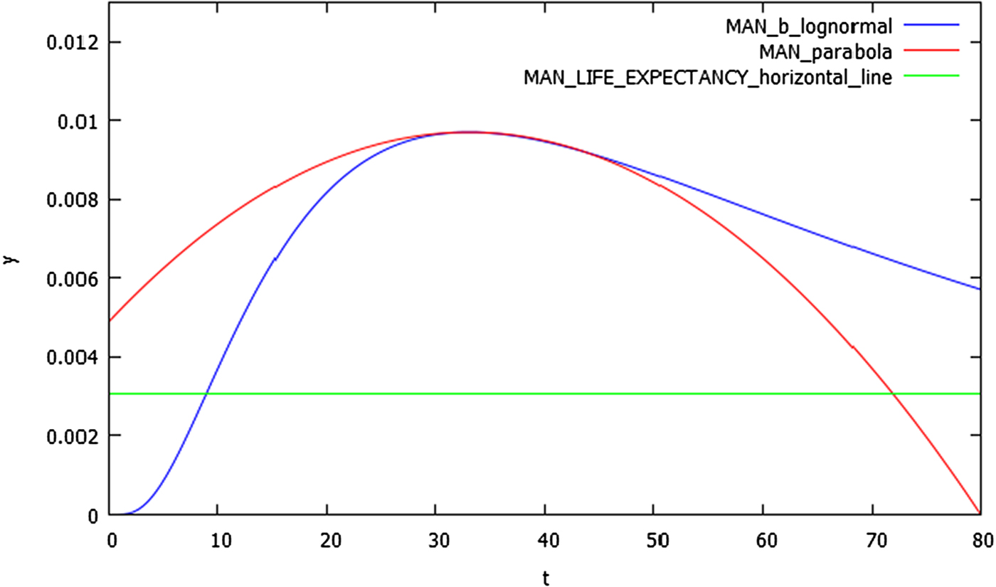
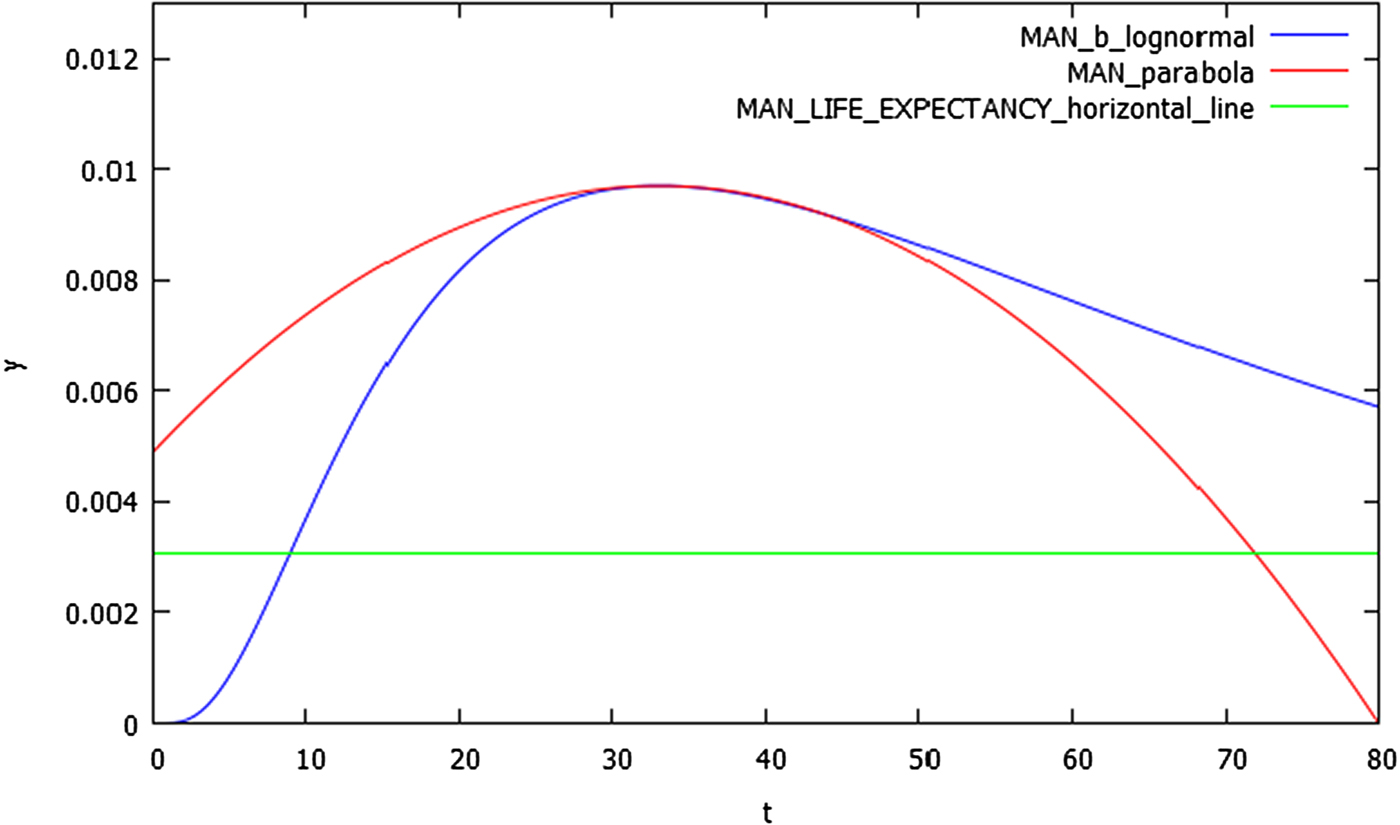
Consider Fig. 2, showing the LOGPAR of a Man's life. In the previous section we only studied the mathematical properties of the b-lognormal's part on the left of the logpar curve. But now we want to extend our mathematical considerations to the right part of the logpar also, that is the parabola.

Fig. 2.

The life of a Man as a LOGPAR power curve. The horizontal axis shows the Man's age in years since his birth. Then, three curves are shown in this graph: (1) The blue b-lognormal departing from birth at time b = 0, intercepting the horizontal green line at the b-lognormal's ascending inflextion point (at 11 years of Man's age), then climbing up to the peak at 33 years of age. Imagine that you do not see the rest of the descending b-lognormal beyond the peak. (2) The red parabola. Imagine that you don't see the first ascending part of the parabola between birth and peak. Then, after the peak, the red parabola plunges down on the right up to the age 80, i.e. the Man's death. (3) The green horizontal line intercepts the ascending b-lognormal at its ascending inflexion point. That is the puberty time for Man, i.e. the beginning of its reproductive capabilities at age 11. Then the horizontal green line continues to the right until it intercepts the red parabola at the End-Of-Fertility time (EOF time). (4) The green line segment in between puberty and EOF time is the FERTILITY Span. (5) The green line segment between birth and death is the LIFE EXPECTANCY.

The first, obvious notion to introduce is that of life expectancy, that is how long a living being may hope to live.

Optimistically, for Humans this might be assumed to be around 80 years, though the numbers change considerably between men and women and according to the different parts of the world. Clearly, the duration of the life expectancy for Humans also depend upon the different economic conditions in which those Humans live. To fix the ideas, we shall assume in this paper

(66)$$(d - b)_{{\rm Man}} = 80\;{\rm years}.$$

When considering the lifetime of a generic Man, as in Fig. 2, it is easier and customary to compute the Man's age starting from his birth, so that in (66) one may set b = 0, changing (66) into

(67)$$d_{{\rm Man}} = 80\;{\rm years}.$$

Introducing the living being's EOF time

Have a look at Fig. 2 again. Since the point of increasing inflexion of the b-lognormal on the left is the puberty time, one may consider the straight line parallel to the time axis, departing from that inflexion point and finally reaching its intercept with the parabola. This intercept we call EOF (End-Of-Fertility) time.

Correspondingly, the segment length between the puberty time and the EOF time is the FERTILITY period of that individual.

And now we cast all that into equations.

First of all, we must determine the abscissa of the EOF time. In other words, we have to equal the ordinate A of the puberty time (i.e. the ascending inflexion point of the b-lognormal on the left) to the parabola intercept on the right and then solve the resulting equation for the intercept time, that is precisely the EOF time. Equating thus (15) to the parabola (9), one gets

(68)$$\displaystyle{{{\rm e}^{ - (\sigma \sqrt {\sigma ^2 + 4} /4) + (\sigma ^2/4) - \mu - (1/2)}} \over {\sqrt {2\pi} \sigma}} = P\left[ {1 - \displaystyle{{{\left( {t - p} \right)}^2} \over {{\left( {d - p} \right)}^2}}} \right].$$

Solving (68) for t one gets the desired EOF time:

(69)$$t_{{\rm EOF}} = p + \left( {d - p} \right)\sqrt {1 - \displaystyle{{{\rm e}^{ - (\sigma \sqrt {\sigma ^2 + 4} /4) + (\sigma ^2/4) - \mu - (1/2)}} \over {\sqrt {2\pi} \,\sigma P}}}. $$

Next, we must let P disappear from (69) by inserting (13) into (69). The result is that μ cancels out in the exponent and, after a little rearranging, one gets

(70)$$t_{{\rm EOF}} = p + \left( {d - p} \right)\sqrt {1 - {\rm e}^{ - \;\textstyle{{\sigma \sqrt {\sigma ^2 + 4} + \sigma ^2 + 2} \over 4}}}. $$

To re-express (70) in terms of b, a and p only, the Adolescence Formula for σ (that is the upper (57)) must be invoked and the conclusion is

(71)$$t_{{\rm EOF}} = p + \left( {d - p} \right)\sqrt {1 - {\rm e}^{\scriptstyle{{ - \,\scriptstyle{{\ln \left( {\scriptstyle{{\,p - b} \over {a - b}}} \right)\sqrt {\scriptstyle{{{\left[ {\ln \left( {\scriptstyle{{\,p - b} \over {a - b}}} \right)} \right]}^2} \over {\ln \left( {\scriptstyle{{\,p - b} \over {a - b}}} \right) + 1}} + 4}} \over {\sqrt {\ln \left( {\scriptstyle{{\,p - b} \over {a - b}}} \right) + 1}}} - \scriptstyle{{{\left[ {\ln \left( {\scriptstyle{{\,p - b} \over {a - b}}} \right)} \right]}^2} \over {\ln \left( {\scriptstyle{{\,p - b} \over {a - b}}} \right) + 1}} - 2} \over 4}}}. $$

This is the abscissa of the intercept between the parabola and the horizontal line drawn from the puberty time. In other words, this is the time when Fertility ends.

Life expectancy of living beings

The Life Expectancy of any living being is how much time that being may expect to live.

In the LOGPAR framework, it is clearly given by the difference between the death time d and the birth time b

(72)$${\rm Life\_Expectancy} = d - b.$$

Fertility span (FS) of living beings

The FS of any living being is the amount of time during which that being has the capability of producing offsprings.

In the LOGPAR framework, this FS is clearly given by the difference between the EOF time and the puberty time. In equations and in terms of μ and σ also, we must subtract (14) to (70), i.e.

(73)$$\eqalign{& {\rm Fertility\_Span = FS = EOF\_time} - a = \cr & \quad = p + \left( {d - p} \right)\sqrt {1 - {\rm e}^{ - \;{{\sigma \sqrt {\sigma ^2 + 4} + \sigma ^2 + 2} \over 4}}} - \cr & \quad \;\; - b + {\rm e}^{ - \,\textstyle{{\sigma \sqrt {\sigma ^2 + 4}} \over 2} - \,\textstyle{{3\sigma ^2} \over 2} + \textstyle\mu}.} $$

The next step is of course the insertion of the Adolescence Formulae (57) into (73) so as to get rid of both μ and σ. The result is the rather awesome but exact equation

(74)$$\eqalign{& {\rm Fertility\_Span = FS} = t_{{\rm EOF}} - a = \cr & \quad = p + \left( {d - p} \right)\sqrt {1 - {\rm e}^{\scriptstyle{{ - \,\scriptstyle{{\ln \left( {\scriptstyle{{\,p - b} \over {a - b}}} \right)\sqrt {\scriptstyle{{{\left[ {\ln \left( {\scriptstyle{{\,p - b} \over {a - b}}} \right)} \right]}^2} \over {\ln \left( {\scriptstyle{{\,p - b} \over {a - b}}} \right) + 1}} + 4}} \over {\sqrt {\ln \left( {\scriptstyle{{\,p - b} \over {a - b}}} \right) + 1}}} - \scriptstyle{{{\left[ {\ln \left( {\scriptstyle{{\,p - b} \over {a - b}}} \right)} \right]}^2} \over {\ln \left( {\scriptstyle{{\,p - b} \over {a - b}}} \right) + 1}} - 2} \over 4}}} - \cr & \quad \;\;\, - \left( {\,p - b} \right) \cdot {\rm e}^{ - \,\scriptstyle{{\ln \left( {\scriptstyle{{\,p - b} \over {a - b}}} \right)\sqrt {\scriptstyle{{{\left[ {\ln \left( {\scriptstyle{{\,p - b} \over {a - b}}} \right)} \right]}^2} \over {\ln \left( {\scriptstyle{{\,p - b} \over {a - b}}} \right) + 1}} + 4}} \over {2\;\sqrt {\ln \left( {\scriptstyle{{\,p - b} \over {a - b}}} \right) + 1}}} - \scriptstyle{{{\left[ {\ln \left( {\scriptstyle{{\,p - b} \over {a - b}}} \right)} \right]}^2} \over {2\;\left[ {\ln \left( {\scriptstyle{{\,p - b} \over {a - b}}} \right) + 1} \right]}}} - b.} $$

Unfortunately, there appear to exist no way to simplify (74) any further.

A numerical example about the most important case: Man

We conclude our discussion about the LOGPAR Life Expectancy and FS by providing a numerical example about the most important case of all: Man.

Suppose that:

1. 1) The Man's age is measured since its own birth. This means to assume that for Man

   (75)$$b_{{\rm Man}} = 0.$$

2. 2) We assume that Puberty occurs at age 11 (though it might be age 10 for girls and 12 for boys)

   (76)$$a_{{\rm Man}} = 11.$$

3. 3) We assume that the peak of Man's activity occurs at age 33 (according to Dante's Divine Comedy!)

   (77)$$p_{{\rm Man}} = 33.$$

4. 4) These are the three input data (‘triplet’) sufficient to make the b-lognormal precise.

5. 5) Now the parabola comes. Clearly, we must assign the death time d, that amounts to what we already called ‘life expectancy’ in (72) (since now b _Man = 0). Optimistically, we will assume that, for a modern and ‘wealthy’ Man, the life expectancy is about 80 years

   (78)$$d_{{\rm Man}} = 80.$$

6. 6) These four assumed inputs (75), (76), (77) and (78) completely determine the μ and σ given by the Adolescence Formulae (57). The relevant numerical values turn out to be

   (79)$$\left\{ {\matrix{ {\;\,\mu _{{\rm LA}}{\rm = 4}{\rm. 071625208175094,}} \cr {\sigma _{{\rm LA}}{\rm = 0}{\rm. 75836511438002}{\rm.}} \cr}} \right.$$

7. 7) The Peak ordinate (13) computed by virtue of the logpar Adolescence Formulae (57) for Man turns out to be

   (80)$$P_{{\rm LA}}=0.011957284676721. $$

8. 8) The Adolescence ordinate a (or Puberty ordinate) is determined via (15) and turns out to equal

   (81)$$A_{{\rm LA}}{\rm = 0}{\rm. 0041872095966534}{\rm.} $$

9. 9) The EOF Time, given by (71), amounts to the numerical value of about 70 years after birth

   (82)$${\rm EO}{\rm F}_{{\rm LA}}{\rm \_time = 70}{\rm. 88734573704019,}$$

10. 10) And, finally, the FS is given by (73) and reads

    (83)$${\rm Fertility\_Span = 59}{\rm. 88734573704019}.$$

With all the above numerical values (let us repeat it: computed by virtue of the Adolescence Formulae (57) and not by virtue of the History Formulae (39)) the resulting logpar plot for Man is given in Fig. 2.

Checking numerically the (small) difference between history formulae and adolescence formulae for man

For all future applications to Astrobiology of the mathematical results described in this paper, it is important to realize that there is no big numerical difference between the numbers given by the History Formulae (39) and the Adolescence Formulae (57).

For instance, in the case of the Man logpar shown in Fig. 2, the Adolescence Formulae (57) yield the numerical values (79) that we repeat here for convenience

(84)$$\left\{ {\matrix{ {\;\,\mu _{{\rm LA}}{\rm = 4}{\rm. 071625208175094,}} \cr {\sigma _{{\rm LA}}{\rm = 0}{\rm. 75836511438002}{\rm.}} \cr}} \right.$$

On the other hand, the History Formulae (39), with the numerical values given by (75), (77) and (78), yield

(85)$$\left\{ {\matrix{ {\;\,\mu _{{\rm LH}}{\rm = 4}{\rm. 236665041781441,}} \cr {\sigma _{{\rm LH}}{\rm = 0}{\rm. 86032405540875}{\rm.}} \cr}} \right.$$

Thus, it plainly appears that the difference among them is conceptual, rather than numeric: the History Formulae are OPTIMIZED by virtue of the condition (30) that the energy must be a minimum, whereas the Adolescence Formulae are not so.