





1. Introduction
Rotating convection is an essential process in, among many other systems, stars (Schumacher & Sreenivasan Reference Schumacher and Sreenivasan2020), protoplanetary disks (Gerbig & Laughlin Reference Gerbig and Laughlin2022), planetary interiors (Aurnou et al. Reference Aurnou, Calkins, Cheng, Julien, King, Nieves, Soderlund and Stellmach2015; Bercovici Reference Bercovici and Schubert2015; Aurnou, Horn & Julien Reference Aurnou, Horn and Julien2020), Earth's atmosphere and oceans (e.g. Emanuel Reference Emanuel1994; Marshall & Schott Reference Marshall and Schott1999; Gayen & Griffiths Reference Gayen and Griffiths2022), and the cryosphere (e.g. Wells & Wettlaufer Reference Wells and Wettlaufer2008; Ravichandran & Wettlaufer Reference Ravichandran and Wettlaufer2021; Cenedese & Straneo Reference Cenedese and Straneo2023). Moreover, rotating Rayleigh–Bénard convection acts as a model system for these phenomena, and the study of pattern formation, such as transient axisymmetric rings observed during spin-up (e.g. Boubnov & Golitsyn Reference Boubnov and Golitsyn1986; Vorobieff & Ecke Reference Vorobieff and Ecke1998; Zhong, Patterson & Wettlaufer Reference Zhong, Patterson and Wettlaufer2010; Ravichandran & Wettlaufer Reference Ravichandran and Wettlaufer2020) and travelling waves observed near the onset of convection (Ecke, Zhong & Knobloch Reference Ecke, Zhong and Knobloch1992; Ning & Ecke Reference Ning and Ecke1993; Liu & Ecke Reference Liu and Ecke1997, Reference Liu and Ecke1999). In typical model studies of rotating Rayleigh–Bénard convection, both theory and numerical simulations employ horizontally periodic domains, whereas experiments do not, leading in part to disagreements. For instance, Rossby (Reference Rossby1969) observed that in rotating Rayleigh–Bénard convection with the typical no-slip experimental boundary conditions, the onset of convection occurs for significantly smaller thermal forcing than predicted by the linear stability analysis of Chandrasekhar (Reference Chandrasekhar1953). Although explanations of this apparent disagreement between theory and experiment can be traced to the basic differences between boundary conditions (BCs) and finite amplitude perturbations (e.g. Veronis Reference Veronis1966, Reference Veronis1968; Herrmann & Busse Reference Herrmann and Busse1993; Kuo & Cross Reference Kuo and Cross1993), there are many interesting outstanding questions (see Ecke Reference Ecke2023). For example, measurements suggest that the peripheral modes may also be responsible for the mismatch between the Nusselt numbers in laboratory experiments and numerical simulations (Kunnen, Clercx & Heijst Reference Kunnen, Clercx and Heijst2013; Wit et al. Reference Wit, Guzmán, Madonia, Cheng, Clercx and Kunnen2020; Ecke, Zhang & Shishkina Reference Ecke, Zhang and Shishkina2022).
In the absence of rotation, the onset of convection in a horizontally unbounded layer of fluid of depth  $H$ across which a temperature difference
 $\Delta T$ is maintained, is governed by the dimensionless Rayleigh number
 \begin{equation} Ra = \frac{g\alpha\Delta T H^3}{\nu \kappa},\end{equation}
where  $g$ is the acceleration due to gravity and
 $\nu$ and
 $\kappa$ are the viscosity and thermal diffusivity of the fluid. The onset of convection occurs when a critical Rayleigh number,
 $Ra_c^{bulk}$, is exceeded, where
 $Ra_c^{bulk} = O(10^3)$, with the exact value depending on the BCs. Chandrasekhar (Reference Chandrasekhar1953) showed that, independent of the Prandtl number
 $Pr=\nu /\kappa$, the instability that leads to convection is non-oscillatory.
Rotation about the vertical axis suppresses the effects of buoyancy and thus enhances stability. Therefore, the critical Rayleigh number increases with the rotation rate,  $\varOmega$, as
 \begin{equation} Ra_c^{bulk} \simeq E^{-4/3} , \end{equation}
where  $E=\nu / 2 \varOmega H^2$ is the Ekman number (Chandrasekhar Reference Chandrasekhar1953; Veronis Reference Veronis1966). In contrast to non-rotating systems, the onset of convection in horizontally unbounded rotating Rayleigh–Bénard convection can be oscillatory if the Prandtl number
 $Pr<0.69$ (Chandrasekhar Reference Chandrasekhar1953).
Rossby (Reference Rossby1969) showed experimentally that convection sets in for much smaller Rayleigh numbers than predicted by (1.2), the possible origins of which were discussed contemporaneously by Veronis (Reference Veronis1968) as being associated with BCs. Of relevance to our study, the experiments by Ecke et al. (Reference Ecke, Zhong and Knobloch1992), supported by linear stability analysis by Goldstein et al. (Reference Goldstein, Knobloch, Mercader and Net1993), showed that the wall-adjacent convection takes the form of a travelling wave with a phase speed opposite to the sense of rotation. They also showed that the system undergoes a Hopf bifurcation at a critical Rayleigh number, following which the travelling wave appears.
Herrmann & Busse (Reference Herrmann and Busse1993) and Kuo & Cross (Reference Kuo and Cross1993) independently showed that, in the asymptotic limit of  $E\rightarrow 0$, the critical Rayleigh number for the onset of the travelling waves in confined rotating Rayleigh–Bénard convection with adiabatic walls is
 \begin{equation} Ra_{cw}^{ZF} = {\rm \pi}^2 (6 \sqrt{3} )^{1/2} E^{-1} = 31.82 E^{-1}, \end{equation}
where the superscript  $ZF$ denotes ‘zero flux’. Herrmann & Busse (Reference Herrmann and Busse1993) also showed that conducting walls stabilize the wall modes, with a critical Rayleigh number that has the same leading order scaling as that for an infinite layer, but with a smaller prefactor,
 \begin{equation} Ra_{cw}^{FT} = 0.9086 ({\rm \pi} E^{-1} )^{4/3} + 2.124 ({\rm \pi} E^{-1} )^{7/6} = 4.18 E^{-4/3} + 8.08 E^{-7/6}, \end{equation}
where the superscript  $FT$ denotes ‘fixed temperature’ highlighting the fact that mathematical well-posedness requires the temperature to be prescribed at a conducting boundary. In their analysis, Herrmann & Busse (Reference Herrmann and Busse1993) assume a wall temperature equal to the purely conductive (linear) profile
 \begin{equation} \bar{T}_{wall} = 1-z. \end{equation}
The flow, for  $Ra > Ra_{cw}^{FT}$, again takes the form of travelling waves that propagate in a retrograde sense, against the sense of rotation.
Instead of the linear temperature boundary condition of Herrmann & Busse (Reference Herrmann and Busse1993), if a constant temperature is imposed across the entire height of the walls, the system is unconditionally unstable with the flow taking the form of wall-adjacent convective rolls. Similar rolls were observed by Ning et al. (Reference Ning, Hu, Ecke and Ahlers1993) for weak thermal forcing at the walls. Constant wall temperatures may be relevant in the melting of ocean-terminating glaciers due to the rotation-influenced convection, wherein the coupling between convective structures and melting morphology could become important (Ravichandran & Wettlaufer Reference Ravichandran and Wettlaufer2021).
For supercritical Rayleigh numbers, the wall modes attain a nonlinear saturated steady state consisting of wall-adjacent regions of upwelling and downwelling flow propagating in a retrograde direction. This nonlinear state has been observed by Lopez et al. (Reference Lopez, Marques, Mercader and Batiste2007), Favier & Knobloch (Reference Favier and Knobloch2020), Zhang et al. (Reference Zhang, Gils, Horn, Wedi, Zwirner, Ahlers, Ecke, Weiss, Bodenschatz and Shishkina2020) and Wit et al. (Reference Wit, Guzmán, Madonia, Cheng, Clercx and Kunnen2020); and Favier & Knobloch (Reference Favier and Knobloch2020) showed it to be robust to severe non-axisymmetric modifications of the geometry. For Rayleigh numbers well beyond the onset of bulk convection, the nonlinear state becomes the so-called boundary zonal flow (see e.g. Wit et al. Reference Wit, Guzmán, Madonia, Cheng, Clercx and Kunnen2020; Zhang et al. Reference Zhang, Gils, Horn, Wedi, Zwirner, Ahlers, Ecke, Weiss, Bodenschatz and Shishkina2020; Ecke et al. Reference Ecke, Zhang and Shishkina2022; Wedi et al. Reference Wedi, Moturi, Funfschilling and Weiss2022), which has been shown to be responsible for significant amounts of heat transfer in rotating Rayleigh–Bénard convection (Wit et al. Reference Wit, Guzmán, Madonia, Cheng, Clercx and Kunnen2020).
Motivated by these findings of the influence of the BCs on the dynamical state of wall modes, here we examine the effects of changing the uniform temperature at which the walls and upper and lower boundaries are held, along with the velocity BCs, as summarized in table 1. We show that the steady roll state undergoes a Hopf bifurcation as a function of the wall temperature, leading to wall modes. The wall temperature at which this onset occurs must be found from linear stability analysis, with the steady rolls as the base state. We study the nonlinear state of the resulting instability, comparing it with the nonlinear state of wall modes with adiabatic walls. We find that the velocity BCs at the upper and lower boundaries control the direction of propagation of the wall modes, and prograde wall modes can arise for suitable velocity BCs. Finally, by studying both cuboidal and cylindrical geometries, we confirm the findings of Favier & Knobloch (Reference Favier and Knobloch2020) that the nonlinear wall mode state is robust to non-axisymmetric geometric modifications.
The combinations of BCs considered. Symmetric (SYMNS) BCs have no-slip upper and lower boundaries, while asymmetric (ASYM) BCs have stress-free upper and no-slip lower boundaries. Consequences of symmetric stress-free (SYMFS) BCs, defined in analogy with SYMNS BCs, and of stress-free BCs at all boundaries (ALLFS) are examined in § 3.2.

The rest of the paper is organized as follows. In § 2, we describe the geometry of the problem and the numerical method used for the simulations. In § 3, we present results from the numerical simulations as the wall temperature, the velocity BC at the upper boundary, the horizontal cross-section of the domain and the Prandtl number are varied, compare our results with other known travelling wave solutions in rotating Rayleigh–Bénard convection, and discuss the effects of asymmetric velocity BCs at the upper and lower boundaries on the direction of propagation of the wall-adjacent spatiotemporal patterns. We conclude in § 4.
2. Set-up and numerical simulations
The domain is a rectangular volume of height  $H$ and width
 $L$, with an aspect ratio
 $\varGamma =L/H=2$, shown schematically in figure 1. The system rotates about the vertical
 $z$ axis with a constant angular velocity
 $\varOmega$.
Our simulations are performed in a cuboidal volume of square cross-section and aspect ratio  $L/H=2$, so that the domain is the region
 $|x|\leq 1, |y|\leq 1$,
 $0\leq z \leq 1$. The walls are either adiabatic or held at a constant temperature. The container rotates about the vertical axis with a constant angular velocity, with gravity pointing vertically down.

We make the Boussinesq approximation, so that fluid properties are assumed to be constant and the flow is assumed to be incompressible. We non-dimensionalize the governing equations using the length scale  $H$ and the buoyancy velocity scale
 $U_b=(g\alpha \Delta T H)^{1/2}$. The non-dimensional governing equations become
 $$\begin{gather} \frac{{\rm D}\boldsymbol{u}}{{\rm D}t} =-\boldsymbol{\nabla} p - \frac{\sqrt{Pr}}{E \sqrt{Ra}} \boldsymbol{e}_z \times \boldsymbol{u}+ \left(\frac{Pr}{Ra}\right)^{1/2}\nabla^{2} \boldsymbol{u}+\boldsymbol{e}_{z}\theta, \end{gather}$$
 $$\begin{gather}\boldsymbol{\nabla}\boldsymbol{\cdot}\boldsymbol{u} =0, \end{gather}$$
 $$\begin{gather}\frac{{\rm D}\theta}{{\rm D}t} = \left(\frac{1}{Ra Pr}\right)^{1/2}\nabla^{2}\theta. \end{gather}$$
We consider the combinations of BCs listed in table 1. The temperature of the lower boundary is fixed at  $\theta (z=0)=1$, the upper boundary at
 $\theta (z=1)=0$ and the walls are either adiabatic (
 $\partial \theta / \partial n = 0$) or have a fixed temperature
 $\theta =\theta _w$, with
 $0\leq \theta _w\leq 1$. The velocity obeys either no-slip or stress-free BCs on the walls at
 $x=\pm 1,y=\pm 1$, and the lower and upper boundaries at
 $z=0$ and
 $z=1$, respectively.
Subject to these BCs, (2.1)–(2.3) are solved using the finite volume solver Megha-5, used in previous studies of convection (Ravichandran & Wettlaufer Reference Ravichandran and Wettlaufer2020, Reference Ravichandran and Wettlaufer2021; Ravichandran, Toppaladoddi & Wettlaufer Reference Ravichandran, Toppaladoddi and Wettlaufer2022). The solver uses second-order central differences in space and a second-order Adams–Bashforth time stepping scheme. Simulations are initialized with broadband noise added to the initial conditions which trigger convection. We use a grid resolution of up to  $256^3$ uniformly spaced points in the three space directions and a time step
 $dt \geq 1.25\times 10^{-3}$. The Nusselt number changes by only a few per cent, with no change in the convection pattern, when the vertical resolution is changed from
 $128$ to
 $256$ grid points; and by approximately
 $0.1\,\%$ when the horizontal resolution is changed from
 $256$ to
 $512$ grid points.
3. Results and discussion
The governing dimensionless parameters of (2.1)–(2.3) are the Ekman ( $E$), Rayleigh (
 $Ra$) and Prandtl (
 $Pr$), numbers as defined above. Simulations are run for a given aspect ratio
 $\varGamma$, and set of BCs. We minimize the amount of computation required by exploring the effects of varying the parameters one at a time around the point;
 $E=10^{-4}, Ra=10^6, Pr=1$, with
 $\varGamma =2$, and
 $0\leq \theta _w\leq 1$. For this combination of
 $E$ and
 $Pr$ in a horizontally unbounded geometry,
 $Ra_c^{bulk}\approx 1.5\times 10^6$, whereas with insulating walls wall modes appear for
 $Ra > Ra_{cw}^{ZF}=3.2\times 10^5$. For walls with the linear temperature profile (see (1.5)),
 $Ra_{cw}^{FT}=1.3\times 10^6$ and for
 $Ra > Ra_{cw}^{FT}$ retrograde propagating wall modes are obtained regardless of the asymmetry in the velocity BCs. This is discussed further in § 3.4.
The initial and BCs described in § 2 lead to the onset of convection everywhere in the domain. The associated bulk flow structure decays away, leaving only the wall attached convection, from which the wall modes emerge and grow into their nonlinear state. The process from which the wall modes emerge from the wall attached convective state involves an instability of a transient base state, and the simulations show a robust and rapid growth into the nonlinear state. Thus, we focus on the latter situation and leave the stability analysis of the secular base state for a standalone study.
3.1. Symmetric and asymmetric velocity BCs
We first examine the flow structures that arise with SYMNS BCs (see table 1) for  $E=10^{-4}, Ra=10^6, Pr=1, \varGamma =2$, while varying
 $\theta _w$. Figure 2 shows that two types of flow may arise; a wall temperature of
 $\theta _w = 0.25$ leads to steady wall-attached rolls in the shape of the container, and
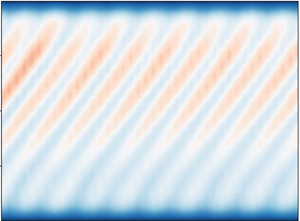
 $\theta _w=0.1$ generates retrograde wall modes. The former are similar to the time-averaged flow seen in the experiments of Ning et al. (Reference Ning, Hu, Ecke and Ahlers1993) at supercritical Rayleigh numbers, with weak thermal forcing at the imperfectly conducting walls. The retrograde propagation of the wall modes is apparent from the space–time Hövmöller diagram in figure 3(a), where we show the near-wall temperature along a horizontal line. Due to the symmetry of the problem, retrograde wall modes with a similar structure are observed for
 $1-\theta _w=0.1$, as seen in figure 3(b). Note that the downward vertical velocity seen in the wall-adjacent region for
 $\theta _w < 0.5$ (figure 2) would be upward were
 $\theta _w > 0.5$.
With  $E=10^{-4}$,
 $Ra=10^6$,
 $Pr=1$ and SYMNS BCs, we see a steady convective state with wall-adjacent rolls for (a,c)
 $\theta_w=0.25$; and wall modes for (b,d)
 $\theta_w=0.1$. The panels show the (a,b) horizontal and (c,d) vertical cross-sections of the vertical velocity
 $w$.

Space–time Hövmöller diagrams of the temperature  $\theta$ for
 $E=10^{-4}, Ra=10^6, Pr=1$; and (a)
 $\theta _w=0.1$ and (b)
 $\theta _w=0.9$. The slope of the patterns shows that the wall modes propagate in a retrograde direction. The symmetry of the Boussinesq equations ensures that the flow patterns for
 $\theta _w$ and
 $1-\theta _w$ are similar. Note that the colour scheme is inverted in (b).

Wall modes are also seen with ASYM BCs for wall temperatures close to upper or lower boundary values, as shown in figure 4. In figure 5, we plot the Hövmöller diagrams for the space–time evolution of the wall modes, showing a reversal of the direction of propagation as follows. For small  $\theta _w = 0.05$, we find retrograde wall modes, as shown in figure 5(a), whereas for large
 $\theta _w = 1$, the wall modes travel in the prograde direction, as shown in figure 5(b). Finally, for intermediate
 $\theta _w$ we find convection in steady rolls, as was the case with SYMNS BCs.
The wall modes observed for  $E=10^{-4}, Pr=1, Ra=10^6$ and ASYM BCs for (a,c)
 $\theta _w=0.05$ and (b,d)
 $\theta _w=1$. The panels show the (a,b) horizontal and (c,d) vertical cross-sections of the vertical velocity
 $w$. In (a,c), the wall modes propagate in the retrograde direction, while in (b,d) they propagate in the prograde direction (see figure 5).

Hövmöller diagrams of the temperature  $\theta$ for the same parameters as in figure 4, showing that for (a)
 $\theta _w=0.05$ the wall modes travel in the retrograde direction, while for (b)
 $\theta _w=1$ they travel in the prograde direction.

Horn & Schmid (Reference Horn and Schmid2017) find flow features that propagate in the prograde direction for small aspect ratios ( $\varGamma =0.5$) with precession frequencies that are comparable to retrograde modes. However, these flow features are ‘bulk modes’, and not restricted to the near-wall region. Horn & Schmid (Reference Horn and Schmid2017) associate their bulk modes with the slow modes of Goldstein et al. (Reference Goldstein, Knobloch, Mercader and Net1993), with precession frequencies much smaller than those of the retrograde modes. Neither of these studies considers the effect of asymmetric velocity BCs, although Goldstein et al. (Reference Goldstein, Knobloch, Mercader and Net1993) do consider conducting walls. Here, we see prograde wall modes with asymmetric velocity BCs, but only for
 $\theta _w \rightarrow 1$, with precession frequencies that are comparable to the usual retrograde modes. In contrast, for insulating walls, the wall modes are retrograde even for asymmetric BCs; and if the wall temperature is very different from that of the no-slip boundary, say
 $\theta _w \lesssim 0.9$, the flow is comprised of nested rolls. In § 3.4, we explain this behaviour by examining the tangential velocity at the walls.
3.2. Additional combinations of BCs
If both the upper and lower boundaries are stress free, and the walls are conducting and obey the no-slip condition (SYMFS BCs, see table 1), wall modes form but they have no clearly discernible direction of propagation. Insulating walls lead to the standard retrograde wall modes, in agreement with earlier studies. Similarly, if both the upper and lower boundaries as well as the conducting walls are stress free (ALLFS BCs), the wall modes that appear have no fixed direction of propagation. Representative snapshots of the wall modes that result from SYMFS and ALLFS BCs are shown in figures 6(a) and 6(b), respectively, with the corresponding Hövmöller diagrams shown in figures 7(a) and 7(b), respectively. A comparison of these figures with the equivalent figures for SYMNS (figures 2 and 3) and ASYM BCs (figures 4 and 5) suggests that while wall modes are observed with conducting walls for suitable wall temperatures  $\theta _w$, no-slip velocity BCs on at least the upper or lower boundaries are necessary for wall modes to propagate in a definite direction. We explain this behaviour by examining the tangential velocity at the walls in § 3.4. Finally, we note that the flow in figure 6 has lost the strong four-fold symmetric structure shown in figures 2 and 4 for SYMNS and ASYM BCs, respectively.
The wall modes observed for  $E=10^{-4}, Ra=10^6, Pr=1$ and (a,c) SYMFS BCs with
 $\theta _w=0.95$ and (b,d) ALLFS BCs with
 $\theta _w=0.1$. The panels show the (a,b) horizontal and (c,d) vertical cross-sections of the vertical velocity
 $w$. The wall modes have no fixed direction of propagation (see also figure 7) and the strong four-fold symmetry seen in figures 2 and 4 is lost.

Hövmöller diagrams of the temperature  $\theta$ for the same parameters as in figure 6, showing that for both (a)
 $\theta _w=0.95$ and SYMFS BCs, and (b)
 $\theta _w = 0.1$ and ALLFS BCs, the wall modes show no fixed direction of propagation.

3.3. Cylindrical geometry
The robustness of wall modes to changes in geometry, observed in the experiments of Ning & Ecke (Reference Ning and Ecke1993) (but not published; see Ecke (Reference Ecke2023)), was studied numerically by Favier & Knobloch (Reference Favier and Knobloch2020). Terrien, Favier & Knobloch (Reference Terrien, Favier and Knobloch2023) observed that wall modes can be suppressed by obstacles (‘fins’) on the boundary by increasing the thermal forcing required for wall mode onset. Here we show the consistency of the flow structures between cuboidal and cylindrical geometries. We also find that the sharp corners in the cuboidal geometry act to dampen the travelling wall modes.
We show the geometry-independence of our findings by performing simulations in a cylindrical geometry of aspect ratio  $D/H=2$ where
 $D$ is the diameter of the cylinder. The cylindrical geometry is embedded in the Cartesian geometry using volume penalization (see Ravichandran & Wettlaufer Reference Ravichandran and Wettlaufer2020), with volume penalization parameters of
 $\eta =5\times 10^{-3}$ or
 $\eta =10^{-3}$ giving the same results. The symmetric (SYM), ASYM and SYMFS BCs are defined in analogy with those in § 2 for the cuboidal geometry, whereas the ALLFS BC cannot be implemented with the solver used here. All other parameters,
 $E=10^{-4}, Pr=1, Ra=10^6$, are unchanged.
In figure 8, we show the steady roll state and retrograde precessing wall modes, which should be compared with those in figure 2. The principal quantitative difference is that the wall temperature  $\theta _c^{(1)}$ up to which wall modes are sustained is larger in the cylindrical geometry for the same Rayleigh number. These wall modes travel in a retrograde or prograde direction for SYM and ASYM BCs, respectively. This is seen in the Hövmöller diagrams in figure 9, for SYMNS and ASYMFS BCs, respectively, showing the influence of asymmetric velocity BCs.
With  $E=10^{-4}$,
 $Ra=10^6$,
 $Pr=1$ and SYMNS BCs in the cylindrical geometry, we see a steady convective state with wall-adjacent rolls for (a,c)
 $\theta_w=0.8$; and wall modes for (b,d)
 $\theta_w=0.95$. The panels show the (a,b) horizontal and (c,d) vertical cross-sections of the vertical velocity
 $w$.

Hövmöller plots of the temperature  $\theta$ for
 $E=10^{-4}, Pr=1, Ra=10^6$ and
 $\theta _w = 0.95$ in the cylindrical geometry shown in figure 8. The direction of propagation is (a) retrograde for SYM BCs and (b) prograde for ASYM BCs.

3.4. Tangential flow velocity at the wall
The reversal in the travel direction of the wall modes may be explained by examining the flow velocity tangential to the walls. The following arguments apply to both the cylindrical and cuboidal geometries.
For SYM velocity BCs, the time-averaged tangential velocity  $\bar {v}$ is plotted in figure 10 for insulating and fixed wall temperatures. Insulating wall BCs give a vertically symmetric tangential velocity that vanishes at the upper and lower boundaries (see also Zhang et al. Reference Zhang, Gils, Horn, Wedi, Zwirner, Ahlers, Ecke, Weiss, Bodenschatz and Shishkina2020). The velocity profiles for conducting walls are starkly different.
With  $E=10^{-4}$,
 $Ra=10^6$,
 $Pr=1$ and SYM velocity BCs, (a) the time-averaged velocity
 $\bar {v}$ tangential to the wall at
 $x=-1$. The velocities are averaged over the region
 $x<-0.9, -0.75< y<1.25$ and over at least
 $300$ flow time units once the wall modes have set in. Large negative (thus prograde) velocities are seen near the upper and lower boundaries for
 $\theta _w=0.9$ and
 $\theta _w=0.1$, respectively; (b) The tangential velocity
 $\bar {v}(x)$ averaged over the region
 $-0.75 < y < 1.25, 0< z<1$. Despite the stark asymmetry in the vertical profiles of velocity for
 $\theta _w=0.1$ and
 $\theta _w=0.9$, the depth-averaged velocity profiles are identical. The positive, and thus retrograde, average tangential velocities are consistent with the retrograde precession of the wall modes for these velocity BCs.

Consider the flow at the wall with  $\theta _w=0.9$. Whereas for the insulating case, there is an inner,
 $O(E^{-1/4})$, Stewartson boundary layer with a prograde velocity, when the walls are at fixed temperature this boundary layer is absent and the velocities at the wall are entirely retrograde. The near-wall flow has a positive vertical velocity and turns inwards at the upper boundary, acquiring a prograde tangential velocity. Flow towards the wall at the lower boundary acquires a retrograde tangential velocity. The stronger buoyancy-forcing at the upper boundary, due to the larger wall-normal thermal gradient, leads to a vertical shear, or thermal wind, resulting in the skewed velocity profiles seen in figure 10(a). These arguments apply when
 $\theta _w=0.1$.
Despite the strong vertical shear seen in figure 10(a), the depth-averaged tangential velocity is retrograde, as shown in figure 10(b). The profiles for  $\theta _w=0.1$ and
 $\theta _w=0.9$, expected to be similar by symmetry, have the same sense as in the case with insulating BCs. In the rotation-dominated flows considered here, wall modes remain vertically coherent, as clearly seen in the three-dimensional contours of figure 11 for both SYM and ASYM BCs, and their precession direction is determined by the depth-averaged tangential velocity, as shown in figure 10(b). Thus, the precession direction of the wall modes is the same for
 $\theta _w=0.1$ and
 $0.9$, and insulating BCs.
Three-dimensional isocontours of the vertical velocity  $w$ for
 $E=10^{-4}, Pr=1, Ra=10^6$ and (a)
 $\theta _w=0.05$ with SYMNS BCs, and (b)
 $\theta _w=0.975$ with ASYM BCs. In both cases, it is evident that the flow structures are columnar, and hence rotation-dominated. The isocontours are plotted for
 $w=0.001$ (red) and
 $w=-0.001$ (blue).

The effects of ASYM BCs are shown in figure 12(a,b), where the vertical profiles for  $\theta _w=0$ and
 $\theta _w=1$ are no longer symmetric about
 $z=0.5$. Owing to the horizontal thermal gradient, the geostrophically balanced flow develops a vertical shear, where the sign of the shear depends on the direction of the thermal gradient. As a result, the depth-averaged velocity profile, which determines the direction of precession, is retrograde for
 $\theta _w=0$ and prograde for
 $\theta _w=1$.
As in figure 10, but with ASYM velocity BCs, showing the tangential velocity  $\bar {v}$ as a function of (a)
 $z$ and (b)
 $x$.

Figures 13(a) and 13(b) show that for SYM BCs the depth-averaged tangential velocity is similar for  $\theta _w=0.25$ (steady rolls) and
 $\theta _w \leq 0.1$ (wall modes). The onset of wall modes for
 $\theta _w \leq 0.1$ is controlled by the vertical shear, which increases with decreasing
 $\theta _w$, rather than by the depth-averaged velocity. For ASYM BCs, the average tangential velocity is prograde, and the vertical shear increases as
 $\theta _w \rightarrow 1$. This argument is bolstered by an examination of the case with the linear wall temperature profile (see (1.5)), wherein the wall thermal forcing is minimal (see Ning & Ecke Reference Ning and Ecke1993), and thus so too is the vertical shear. Therefore, the net tangential velocity is retrograde and the wall modes propagate in the retrograde direction for both SYM and ASYM velocity BCs. These arguments apply in both cuboidal and cylindrical geometries.
The tangential velocity as a function of (a,c)  $z$ and (b,d)
 $x$ for cases where the flow takes the form of rolls and wall modes for (a,b) SYM and (c,d) ASYM BCs with fixed wall temperatures
 $\theta _w$. The combination of the depth-averaged tangential velocity and the vertical shear dictate the onset of wall modes from the steady roll state. Flow parameters are as in figures 10 and 12.

For ALLFS and SYMFS BCs, wall modes have no preferred direction of travel. In figure 14 we see that, compared with the case with insulating walls, fixed-temperature walls lead to much smaller depth-averaged tangential velocities of indeterminate direction. The latter point is demonstrated by comparing the two different realizations of the ALLFS BCs.
As in figures 10 and 12, but with SYMFS and ALLFS velocity BCs. Despite the large tangential velocities at the upper and lower boundaries seen in (a), the depth-averaged velocities in (b) are of much smaller magnitudes.

Lastly, figure 15 shows the tangential velocity profiles obtained with the linear wall temperature (see (1.5)), no-slip BCs on the lower boundary at  $z=0$ and either no-slip or stress-free BCs on the upper boundary at
 $z=1$. Since the thermal forcing at the wall is smaller than for fixed
 $\theta _w$, the vertical shear generated is negligible, and the average tangential velocity is retrograde. The wall modes propagate in a retrograde direction for both velocity BCs.
Tangential velocity profiles versus (a)  $z$ and (b)
 $x$, for the cases with the linear wall temperature of (1.5).

3.5. The influence of  $\theta _w$ on wall mode formation

From the results presented in §§ 3.1 and 3.2, we see that wall modes only occur for values of  $\theta _w$ sufficiently close to the upper or lower boundary temperatures, with the flow taking the form of steady rolls for
 $\theta _w > \theta _c^{(1)}$ (see figure 2a,c). To determine the wall temperature
 $\theta _c^{(1)}$ below which wall modes exist,
 $\theta _w < \theta _c^{(1)}$, we quantify the wall mode strength using the oscillation amplitude of the temperature
 $\theta (x,y,z,t)$ as
 \begin{equation} {A_\theta^2 = \langle (\theta - \bar{\theta} ) ^ 2 \rangle,} \end{equation}
where  $\bar {\theta }(x,y,z)$ is the time-averaged temperature at a given location
 $(x,y,z)$, and the angle brackets
 $\langle {\cdot } \rangle$ denote an average over the spatial domain. Thus, the amplitude
 $A_\theta =0$ for steady (or zero) flow, and the wall temperature
 $\theta_{w}$ at which
 $A_\theta > 0$ is the critical wall temperature
 $\theta _c^{(1)}$. Similarly, the temperature
 $\theta _c^{(2)}$ is defined such that when
 $\theta _w > \theta _c^{(2)}$ wall modes occur, and when
 $\theta _w < \theta _c^{(2)}$, steady convective rolls occur.
In figure 16, we plot the oscillation amplitude  $A_\theta$ as the wall temperature
 $\theta _w$ is varied for SYMNS BCs and fixed flow parameters
 $E=10^{-4}, Ra=10^6$, and
 $Pr=1$. We find that the domain-averaged oscillation amplitude
 $\bar {A}_\theta ^2 \propto |\theta _w-\theta _c^{(1)}|$, with a critical wall temperature
 $\theta _c^{(1)} \approx 0.1$. This dependence of the amplitude on the deviation from threshold is similar to the Hopf bifurcation that occurs for wall modes with insulating walls (Ecke et al. Reference Ecke, Zhong and Knobloch1992), in which the controlling parameter is the Rayleigh number.
(a) The amplitude  $A_\theta ^2$ of the wall modes as a function of time, showing the existence of a steady oscillatory state and (b) the domain-averaged oscillation amplitude
 $\bar {A}_\theta ^2$ as a function of the reduced wall temperature
 $\theta _w / \theta _c^{(1)} - 1$ for SYMNS BCs (see table 1) and fixed flow parameters
 $E=10^{-4}, Ra=10^6$ and
 $Pr=1$. In the inset of (b),
 $A_\theta ^2$ is plotted versus the wall temperature
 $\theta _w$. The curves in (a) are plotted for the wall temperatures
 $\theta _w = (0, 0.05, 0.1, 0.1125, 0.125, 0.15, 0.25)$, with circles of larger size for smaller
 $\theta _w$. The averages in (b) are obtained over the last
 $100$ flow units of each curve in (a). The linear dependence of the (squared) amplitude on the magnitude of the deviation from the critical wall temperature is characteristic of a Hopf bifurcation.

We repeat this exercise for different values of  $Ra$, keeping the parameters
 $E=10^{-4}$ and
 $Pr=1$ fixed. The smallest value of
 $Ra$ such that
 $\theta _c^{(1)}(Ra) > 0$ is defined as
 $Ra_c^{(1)}=Ra_c^{(1)}(E,Pr,{BCs})$. The resulting behaviour for the cases we have simulated is summarized schematically in figure 17, where we find a monotonic dependence of
 $\theta _c^{(1)}$ on
 $Ra$. For SYMNS BCs and wall temperatures
 $\theta _w < \theta _c^{(1)}$ and
 $\theta _w > \theta _c^{(2)}$ retrograde wall modes are observed as seen in figures 3(a) and 3(b), respectively. The difference
 $\theta _c^{(2)}-\theta _c^{(1)}$ decreases monotonically as
 $Ra$ increases.
The different regimes of behaviour observed with conducting walls and SYMNS BCs. The symbols denote whether wall modes (circles), steady rolls (squares) or bulk convection with columnar vortices (crosses) are seen. Note that combinations of these are possible. The regions shaded grey and blue correspond to the steady roll- and bulk-convective states. The lower and upper boundaries of the grey region correspond to the critical temperatures  $\theta _c^{(1)}$ and
 $\theta _c^{(2)}$, respectively. For small Rayleigh numbers
 $Ra$, wall-attached steady rolls are seen for all
 $\theta _w$. For Rayleigh numbers greater than a critical value
 $Ra_c^{(1)}$, wall modes are seen for
 $\theta _w < \theta _c^{(1)}$ and
 $\theta _w > \theta _c^{(2)}$, while the steady roll state persists for
 $\theta _c^{(1)} < \theta _w < \theta _c^{(2)}$. For larger Rayleigh numbers, convection also sets in away from the walls, with the flow taking the form of a series of nested rolls that remain stable for extended periods of time. For
 $Ra > Ra_c^{(2)}\equiv Ra _c^{bulk}$ of (1.2), flow in the bulk takes the form of horizontally drifting columnar vortices that are typical of rotating Rayleigh–Bénard convection, while either nested rolls or wall modes are seen adjacent to the walls. For
 $E=10^{-4}, Pr=1$, we find
 $Ra_c^{(1)}=9\times 10^5$, and
 $Ra_c^{bulk}=1.5\times 10^6$.

As the Rayleigh number approaches the critical value for the onset of bulk flow,  $Ra_c^{bulk}=1.5\times 10^6$ from (1.2), the difference
 $\theta _c^{(2)}-\theta _c^{(1)}$ can either (i) vanish before bulk flow sets in, such that
 $Ra_c^{(2)} < Ra_c^{bulk}$, or (ii) remain finite until bulk convection sets in at
 $Ra_c^{(2)} = Ra_c^{bulk}$. We find the latter case, wherein as
 $Ra$ increases the flow takes the form of a series of nested convection rolls that span the entire horizontal area of the domain, as shown in figure 18(a,d). For
 $Ra > Ra_c^{bulk}$, as noted above, these rolls break down into individual columnar vortices in the fluid bulk, as seen in figure 18(b,e), due to the mechanism reported by Boubnov & Golitsyn (Reference Boubnov and Golitsyn1986), Zhong et al. (Reference Zhong, Patterson and Wettlaufer2010) and Ravichandran & Wettlaufer (Reference Ravichandran and Wettlaufer2020), into a state of geostrophic convection in the bulk. For larger
 $Ra$, the wall modes become less prominent.
With  $E=10^{-4}, Pr=1, \theta _w=0.4$ and SYMNS BCs, we see (a,d) for
 $Ra=Ra_c^{bulk}=1.5\times 10^6$, steady nested rolls spanning the entire horizontal extent of the domain; (b,e) wall-adjacent steady rolls with columnar vortices in the bulk for
 $Ra=1.6\times 10^6$. Note that for
 $\theta _w=0.25 < \theta _c^{(1)}$, we see (c,f) bulk convection coexist with retrograde propagating wall modes. See also figure 17.

The symmetry between  $\theta _c^{(1)}$ and
 $\theta _c^{(2)}$ observed for SYMNS BCs, where
 $\theta _c^{(1)} + \theta _c^{(2)} = 1$, breaks down if the velocity boundary conditions are asymmetric, such as for ASYM BCs. In figure 19, we plot the oscillation amplitude
 $A_\theta ^2 (\theta _w)$ for the same parameters as in figure 16, but with ASYM BCs, showing that
 $\theta _c^{(1)} + \theta _c^{(2)} > 1$.
(a) The amplitude  $A_\theta ^2$ of the spatiotemporal oscillations as a function of time, showing the existence of a steady oscillatory state, and the domain-averaged oscillation amplitude
 $\bar {A}_\theta ^2$ as a function of (b) the reduced wall temperature
 $\theta _w / \theta _c^{(1)} - 1$, and (c)
 $\theta_w / \theta_c^{(2)} - 1$, for ASYM BCs (see table 1). In the inset of (b),
 $A_\theta ^2$ is plotted versus the wall temperature
 $\theta _w$. The curves in (a) are plotted for the wall temperatures
 $\theta _w = (0, 0.05, 0.1, 0.15)$ (solid lines, circles of decreasing size) and
 $\theta _w= (0.85, 0.9, 0.95, 0.975, 1.0)$ (dashed lines, squares of increasing size). The averages in (b) are obtained over the last 100 flow units for each curve in (a). The linear dependence of the (squared) amplitude on the magnitude of the deviation from the critical wall temperature is characteristic of a Hopf bifurcation. Note the asymmetry between
 $\theta _c^{(1)}$ and
 $\theta _c^{(2)}$ (c.f. figure 16).

Of further relevance to figure 17 is the fact that in the limit  $E\rightarrow 0$, (1.3) and (1.4) for the critical Rayleigh numbers are independent of the Prandtl number. For finite
 $E$, Herrmann & Busse (Reference Herrmann and Busse1993) found that as the Prandtl number decreased so too did
 $Ra_c$ (see their figures 3 and 6), driving the system towards instability. Similarly, decreasing the Ekman number increases the critical Rayleigh number, and leads to the same qualitative effects as does decreasing
 $Ra$. Next, we consider further the effects of varying the Prandtl number.
3.6. The role of the Prandtl number
An important effect of varying the Prandtl number to control the thickness of the thermal boundary layers at the walls and the resultant heat transfer. Thus, for a Boussinesq fluid, decreasing the Prandtl number is associated with increasing the thermal diffusivity.
Considering again the case of  $\theta _w \approx 1$, with other parameters held constant, smaller Prandtl numbers result in larger buoyancy forcing at the walls, leading to larger wall-adjacent vertical velocities, and larger retrograde velocities as the flow turns inwards at the upper boundary. As a result, the flow experiences greater vertical shear, which results in the onset of wall modes for a smaller
 $\theta _w$. We see in figure 20 that decreasing
 $Pr$ and increasing
 $Ra$ both increase
 $\theta _c^{(1)}$. Thus, for
 $Pr = 0.5$, wall modes are seen for
 $\theta _w=0.15$ in figure 21(a), whereas steady rolls are seen for
 $Pr=1$. In contrast, for
 $Pr=2$, the steady roll state is seen for
 $\theta _w=0$ in figure 21(b), and larger values of
 $Ra$ are needed for the onset of wall modes than for the onset of bulk convection. Therefore, smaller Ekman numbers, and thus more strongly rotation-dominated flows, are needed for wall modes when
 $Pr>1$.


With  $E=10^{-4}$,
 $Ra=10^6$ and SYMNS BCs, we see wall modes for (a,c)
 $Pr=0.5$ and
 $\theta_w=0.15$; and a steady convective state with wall-adjacent rolls for (b,d)
 $Pr=2$ and
 $\theta_w=0$. The panels show the horizontal (a,b) and vertical (c,d) cross-sections of the vertical velocity
 $w$.

4. Conclusion
The flow structure in confined rotating Rayleigh–Bénard convection is comprised of alternating regions of upwelling warm and downwelling cold fluid. When conditions lead to these patterns being adjacent to the walls of the system, they are commonly referred to as ‘wall-modes’, and were first observed in laboratory experiments (see Rossby (Reference Rossby1969), Ecke et al. (Reference Ecke, Zhong and Knobloch1992), and references in the latter). Here, in geometries of aspect ratio greater than unity, we have used direct numerical simulations to study the formation and spatiotemporal evolution of wall-adjacent flow patterns when the walls are conducting instead of insulating. We showed that the wall temperature  $\theta _w$ controls whether the flow takes the form of steady convective rolls or propagating wall-modes. We found that the velocity BCs are crucial to the dynamics of wall modes, and that these modes propagate in a fixed direction only if at least one of the upper and lower boundaries obeys the no-slip condition. Moreover, the direction of propagation of the wall modes can be reversed for suitable combinations of the velocity BCs at the upper and lower boundaries and the wall temperature. In particular, if only the upper boundary is stress free, the wall modes propagate in a prograde direction when
 $\theta _w \approx 1$. Indeed, there is a similarity between the effects of velocity BCs on wall mode formation and propagation, to transient convective ring formation (Boubnov & Golitsyn Reference Boubnov and Golitsyn1986; Vorobieff & Ecke Reference Vorobieff and Ecke1998; Zhong et al. Reference Zhong, Patterson and Wettlaufer2010; Ravichandran & Wettlaufer Reference Ravichandran and Wettlaufer2020).
Although wall modes were previously shown to occur when the walls are conducting, we found that asymmetric velocity BCs drive an asymmetry in the torques exerted at the two boundaries. Such effects may have astrophysical or geophysical consequences, where asymmetric velocity BCs are common, such as for example in natural bodies of water with free upper surfaces. The effects of the asymmetry in velocity BCs on integral flow properties, such as the helicity (Moffatt & Tsinober Reference Moffatt and Tsinober1992) are a subject of ongoing study.
Finally, the rich range of flow behaviour in slightly supercritical Rayleigh–Bénard convection has served as a model for the study of nonlinear-dynamical systems, such as the Benjamin–Feir and Eckhaus instabilities (Ning & Ecke Reference Ning and Ecke1993; Liu & Ecke Reference Liu and Ecke1997, Reference Liu and Ecke1999; Lopez et al. Reference Lopez, Marques, Rubio and Avila2009). More recent studies have shown that the wall-modes in rotating Rayleigh–Bénard convection may be a topologically conserved feature, robust to severe vertically homogeneous modifications to the geometry (Favier & Knobloch Reference Favier and Knobloch2020). Therefore, the influence of conducting walls in combination with asymmetric velocity BCs on the wall modes may provide a framework of general interest in the theory of pattern formation.
Acknowledgements
We thank the anonymous referees for helpful comments.
Funding
Computational resources from the Swedish National Infrastructure for Computing (SNIC) under grants SNIC/2020-5-471, SNIC/2021-5-449 and SNIC/2022-5-473 are gratefully acknowledged. Computations were performed on Tetralith. The Swedish Research Council, under grant no. 638-2013-9243, is gratefully acknowledged for support. Nordita is partially supported by Nordforsk. Since July 2022, S.R. has been supported through Seed Grant RD/0522-IRCCSH0-020 from IIT Bombay.
Declaration of interests
The authors report no conflict of interest.


 Open access

