
I. INTRODUCTION
Understanding solidification is the key to many aspects of the microstructure of nickel base superalloys, and is thus also directly or indirectly related to the resulting mechanical properties of this important class of materials. Reference Reed1 In recent years, progress has also been made in addressing technologically relevant aspects of microstructure formation during solidification using computer simulations within the emerging field of integrated computational materials engineering. Certainly, this would not be possible without the strong basis of dendritic growth theory.
Since the fundamental discovery of a steady state solution to the problem of diffusion-limited solidification in the free space by Ivantsov, Reference Ivantsov2 it took quite a long time to finally understand that the interfacial energy, and in particular its anisotropy, both play a central role in dendritic growth Reference Brener and Mel’nikov3,Reference Danzig and Rappaz4 : In the classical case, it is the anisotropy of the interfacial energy which determines the growth direction, the dendritic tip-radius as well as the growth velocity all together within the so-called dendritic selection. However, apart from the rather weak interface energy anisotropy, other anisotropic physical effects can also provide such a selection of stationary diffusion-limited growth patterns in the free space. Reference Brener, Boussinot, Huter, Fleck, Pilipenko, Spatschek and Temkin5 In the special case of a purely isotropic interfacial energy and no further anisotropic physical effect present in the system, stationary dendritic-type solutions do not even exist and instead unsteady see-weed or directionally unstable doublon structures emerge in the free space. Reference Ben Amar and Brener6,Reference Ihle and Müller-Krumbhaar7 With regard to the present purpose of solidification modeling, we additionally consider the influence from the anisotropy of the interface kinetics. This has been found to be quite important in the context of rapid solidification modeling in metallurgy. Reference Danzig and Rappaz4,Reference Turnbull8 Atomistic simulations of the solid/liquid interface in pure nickel further revealed this interface property—i.e., the interface attachment kinetics—to be quite strongly anisotropic. Reference Huitema, Vlot and van der Eerden9,Reference Bragard, Karma, Lee and Plapp10
Also an important aspect in the discussion of solidification modeling is to distinguish between confined and free growth, i.e., to account for the effect from a finite simulation domain on the resulting growth morphology. Confined stationary growth is usually discussed within a channel geometry, where the dendritic tip is growing within an at least thought to be infinitely extended channel. Of course, the channel boundaries on each side of the dendritic tip have a tremendous influence on the dendritic solidification, as they determine the basic growth direction. In fact, it is known that the channel boundaries provide a whole number of different steady states to the problem of confined diffusion-limited growth. Reference Ben Amar and Brener6,Reference Kupferman, Kessler and Ben-Jacob11 Those steady-state solutions in the channel have also been studied recently using the phase-field method. Reference Sabouri-Ghomi, Provatas and Grant12–Reference Kassner, Guérin, Ducousso and Debierre15 However, we point out that the discussion of steady state solutions in the channel has also limited relevance for the usual experimental situation of unconstrained solidification. Typically, one imposes mirror-type boundary conditions at the channel walls, to also effectively study the growth of a periodic array of dendritic tips. Reference Gurevich, Karma, Plapp and Trivedi16,Reference Ma and Plapp17
Phase field modeling of alloy solidification has been studied extensively throughout the last decade, and there are numerous reviews available. Reference Boettinger, Warren, Beckermann and Karma18,Reference Asta, Beckermann, Karma, Kurz, Napolitano, Plapp, Purdy, Rappaz and Trivedi19 The physical solid/liquid interface for metals and alloys is finite but of small width (typically in the range of a few nm). This finite interface width comes along with a number of physical effects, which are somewhat automatically contained in any diffuse interface descriptions such as the phase field method. The most prominent and also technically most relevant of these effects is certainly the effect of solute trapping. Reference Boettinger, Warren, Beckermann and Karma18 Although all these effects are real physical effects, they are spuriously enhanced in usual phase-field simulations of the microstructure evolution due to a necessary overestimation of the interface width. This topic has been extensively discussed under the keyword thin interface asymptotic analysis, which was pioneered by Karma and coworkers for modeling solidification in pure substances (equal diffusivity in the solid and the liquid). Reference Bragard, Karma, Lee and Plapp10,Reference Karma and Rappel20 It turned out, however, that the generalization of this method to a model with arbitrary diffusivities is far from trivial Reference Almgren21 since several new thin-interface effects appear, which cannot all be eliminated simultaneously. A solution to this problem was found later for the case of the one-sided model (zero diffusivity in the solid) with the introduction of the so-called anti-trapping current. It was shown that quantitative simulations of alloy solidification are possible with this model, Reference Echebarria, Folch, Karma and Plapp22 including multiphase Reference Folch and Plapp23 and multicomponent alloys. Reference Kim24 Nevertheless, eliminating all the spuriously enhanced effects in the case of finite diffusion contrast has remained to be a quite challenging task. Reference Ma and Plapp17,Reference Plapp25 However, recently, there has been a very promising attempt tackling the problem from a different perspective by Brener and coworkers. Reference Brener and Boussinot26,Reference Boussinot, Brener, Hüter and Spatschek27 They have introduced an Onsager kinetic cross-coupling between nonconserved phase field and the conserved concentration field. Reference Brener and Boussinot26 The importance of the new terms has been evidenced for important physical phenomena such as the solute trapping effect Reference Brener and Boussinot26 or the surface diffusion. Reference Boussinot, Brener, Hüter and Spatschek27
Within this article, we develop a phase field model for the simulation of chemically diffusion-limited solidification in multicomponent alloys. The solid/liquid phase transformation is driven by a simplified parabolic thermodynamic description, which can be fitted to a CALPHAD multiphase equilibrium. The solid/liquid interface is considered to be anisotropic with regard to capillarity (interface energy) as well as kinetics. Here, attention has been payed to allow the independent choice of the kinetic anisotropy strength and the strength of the anisotropy of the interfacial energy. With respect to the chemical multicomponent diffusion, we restrict to the case of symmetric diffusion, where the diffusivities are considered to be equal in the solid and liquid phase. This should be seen as the necessary first step toward quantitative modeling of solidification. Here, we aim at the investigation of the basic qualitative aspects of phase-field solidification modeling in multicomponent alloys. More complicated and advanced modeling techniques like for instance the above mentioned thin interface corrections or kinetic cross couplings are not included in the model so far.
The model is applied to the simulation of solidification in the well-known nickel base superalloy Inconel 718. Respective temperature-dependent thermodynamic and kinetic input data have been generated using the ThermoCalc- and DICTRA-module of the respective commercial CALPHAD software-package in conjunction with the thermodynamic database TTNi8 and the kinetic database MobNi1. 28 Specifically, we focus on the investigation of stationary isothermal and directional solidification. The, respectively, modeled solidification behavior obtained from the two different configurations is compared.
Therefore, we proceed as follows: In Sec. II, we present the phase field model. First, the modeling equations are derived in Sec. II.A and then details on the specific simulation configurations as well as the respective scaling are provided in Sec. II.B. After that, in Sec. III, the results on the simulation of solidification in the Inconel 718 superalloy is presented. Here, we begin with the discussion on the simulations of isothermal and directional solidification with a planar front, within a one dimensional simulation domain (see Sec. III.A). This is followed by the discussion on the generation of the scaling parameters for the proceeding simulations as well as their relation to real measures in Inconel 718 in Sec. III.B. After that, in Sec. III.C, we present the simulation studies on isothermal and directional solidification in two-dimensional domains. Finally, in Sec. IV, we give a short conclusion.
II. PHASE-FIELD MODELING OF SOLIDIFICATION
A. The derivation of the model equations
We consider the solidification to be driven by an equilibrated external temperature field. The assumption of instantaneous thermal equilibration during the proceeding solidification is legitimated, if the temperature does not undergo the solidus temperature of the material, i.e., the so-called chemical diffusion-limited growth regime. The reason for this is that the diffusional transport of chemical elements is typically a few orders of magnitude slower than the transport of latent heat. The phase field model for the simulation of solidification is based on a phenomenological grand canonic potential functional,
 $$\Omega = \int_V {\left( {{\omega _{{\mathop{\rm int}} }} + {\omega _{{\rm{bulk}}}}} \right){\rm{d}}V} \quad .$$
The total grand potential density splits into the interfacial contribution ωint(φ, ∇φ) and the bulk chemical contribution ωbulk(φ, {μ i }, T). The interfacial contribution depends on the phase field φ and the phase field gradient ∇φ, whereas the bulk chemical contribution depends on the phase field φ, the multiple chemical diffusion potentials {μ i } as well as the temperature T. In principle, also an elastic grand potential contribution can be included as well, as shown in Refs. Reference Eggleston, McFadden and Voorhees31 and Reference Debierre, Karma, Celestini and Guérin32. However, with regard to the simulation of solidification, as considered here, elastic effects are not important. The interfacial contribution to the grand potential functional is given by
 $${\omega _{{\mathop{\rm int}} }} = 3\Gamma \cdot a\left( {{\varepsilon _{\rm{c}}},{\bf{n}}} \right)\left( {{\xi \over 4}\left( {{\partial _{\rm{l}}}\varphi {\partial _{\rm{l}}}\varphi } \right) + {4 \over \xi }g\left( \varphi \right)} \right)\quad ,$$
where we make use of Einsteins sum convention, i.e., the summation over repeated indices is not explicitly written, and ∂ i denotes an abbreviation for the partial derivative with respect to the spacial direction x i i.e., ∂ i ≡ ∂/∂x i . Further, g(φ) = φ2(1 − φ)2 denotes the double-well potential, guaranteeing that the potential energy density has distinct minima at φ = 0 and φ = 1, which correspond to the two possible phases of the system. The parameter Γ corresponds to the mean interfacial energy density, and ξ determines the width of the transition region, where the phase field φ changes from 0 to 1 or vice versa. Finally, a(εc, n) corresponds to the dimensionless anisotropy function, with εc denoting the strength of the anisotropy of the interface energy density. The anisotropy function is given by the following 4-fold symmetric expression Reference Plapp25
 $$a\left( {{\varepsilon _4},{\bf{n}}} \right) = 1 - 3{\varepsilon _4} + 4{\varepsilon _4}\left( {n_i^2n_i^2} \right)\quad ,$$
with n i = ∂ i /|∇φ| denoting the unit vector pointing in a direction normal to the phase boundary. As usual, the strength of anisotropy is characterized by the parameter ε4 that can be measured experimentally by examining the deviation of the equilibrium particle shape from a sphere. Reference Plapp25 The equation of motion for the phase field is given by the dissipative Allan–Cahn ansatz
 $${{3\Gamma \xi } \over {2M \cdot {a_{\rm{s}}}\left( {{\varepsilon _{\rm{k}}},{\bf{n}}} \right)}}{{\partial \varphi } \over {\partial t}} = - {{\delta \Omega } \over {\delta \varphi }} = {\partial _i}\left( {{{\partial {\omega _{{\mathop{\rm int}} }}} \over {\partial \left( {{\partial _i}\varphi } \right)}}} \right) - {{\partial {\omega _{{\mathop{\rm int}} }}} \over {\partial \varphi }} - {{\partial {\omega _{{\rm{bulk}}}}} \over {\partial \varphi }}\quad ,$$
where M is the mean kinetic coefficient with the physical dimension m2/s. Note that also the interface kinetics is considered to be anisotropic, with the dimensionless anisotropy strength εk and the interface orientation dependence given again by Eq. (3). Therefore, in our model, the anisotropy of the solid/liquid interface is determined by two independent parameters, the capillary εc and the kinetic anisotropy strength εk, which are in general different. For further details of the anisotropic formulation, see Refs. Reference Karma and Rappel20 and Reference Eggleston, McFadden and Voorhees31–Reference Fleck, Mushongera, Pilipenko, Ankit and Emmerich33.
For a nonisothermal, multi-component, and multi-phase system, we formulate the multicomponent and multiphase thermodynamics on the basis of quadratic Gibbs free energy density functions similar to Ref. Reference Heulens, Blanpain and Moelans34. The concentration-dependent Gibbs free energy density of the phase α is approximated by the following expression:
 $$g_{{\rm{ch}}}^\alpha \left( {\left\{ {{c_i}} \right\},T} \right) = {1 \over 2}\left( {{c_i} - A_i^\alpha } \right)X_{ij}^\alpha \left( {{c_j} - A_j^\alpha } \right) + {B^\alpha }\quad ,$$
where
 $X_{ij}^\alpha$
denotes the thermodynamic factor. Note, that Einsteins summation convention is again applied for the summation over the different chemical elements and the imposed constants defining the parabolic energy density are all subjected to an implicit temperature dependence, i.e.,
 $A_i^\alpha \left( T \right)$
, B
α(T),
 $X_{ij}^\alpha \left( T \right)$
. As indicated in Eq. (5), the Gibbs free energy density naturally depends on the multiple concentrations, {c
i
}, as well as the temperature T. In contrast to this, the natural variables of the grand potential density are the temperature together with the multiple diffusion potentials {μ
i
}. The later are defined as the partial derivatives of the Gibbs free energy density with respect to the different concentrations, i.e.,
 ${\mu _i} = \partial g_{{\rm{ch}}}^\alpha {\rm{/}}\partial {c_i} = X_{ij}^\alpha \hbox( {{c_j} - A_j^\alpha } \hbox)$
. Then the grand-potential density is obtained from the Gibbs free energy density by means of the following Legendre transformation
 $$\omega _{{\rm{ch}}}^\alpha \left( {\left\{ {{\mu _i}} \right\}} \right) = g_{{\rm{ch}}}^\alpha - {\mu _i}{c_i}\quad {\rm{with}}\quad {c_i} = \chi _{ij}^\alpha {\mu _j} + A_i^\alpha \quad ,$$
where
 $\chi _{ij}^\alpha = \left( {{X^\alpha }} \right)_{ij}^{ - 1}$
is the inverse of the thermodynamic factor matrix, a generalized susceptibility.
Reference Plapp35
Note that for metallic alloys at atmospheric pressure, the Gibbs free energy can be treated as equal to the free energy. The temperature-dependent constants
 $A_i^\alpha \left( T \right)$
, B
α(T), and
 $X_{ij}^\alpha \left( T \right)$
can be determined from the two-phase equilibrium, which is calculated using the CALPHAD method. We obtain the following equations relating
 $A_i^\alpha$
and B
α with the two-phase equilibrium concentrations
 ${\hbox( {c_{{\rm{eq}}}^\alpha } \hbox)_i}$
, the diffusion potentials (μeq)
i
, and the Gibbs free energies
 $g_{{\rm{eq}}}^\alpha$
.
Reference Mushongera, Fleck, Kundin, Wang and Emmerich29,Reference Mushongera, Fleck, Kundin, Querfurth and Emmerich30
 $$A_i^\alpha = {\left( {c_{{\rm{eq}}}^\alpha } \right)_i} - \chi _{ij}^{\rm{\alpha }}{\left( {{\mu _{{\rm{eq}}}}} \right)_j}\quad ,$$
 $${B^\alpha } = g_{{\rm{eq}}}^\alpha - {1 \over 2}\chi _{ij}^\alpha {\left( {{\mu _{{\rm{eq}}}}} \right)_i}{\left( {{\mu _{{\rm{eq}}}}} \right)_j}\quad .$$
The total chemical grand potential density from Eq. (1) is defined to be
 ${\omega _{{\rm{bulk}}}} = h\left( \varphi \right)\omega _{{\rm{ch}}}^\alpha + h\left( {1 - \varphi } \right)\omega _{{\rm{ch}}}^\beta$
, where φ = 1 denotes the α-phase and φ = 0 the β-phase. h(φ) = φ2(2 − 3φ) is the interpolation function, which is the minimal polynomial function satisfying the necessary interpolation condition, h(0) = 0, h(1) = 1, and having also a vanishing slope at zero and one, i.e., ∂h(φ = 0, 1)/∂φ = 0, for not to shift the two minima in case of finite driving forces.
Reference Fleck, Mushongera, Pilipenko, Ankit and Emmerich33,Reference Kassner, Misbah, Müller, Kappey and Kohlert36,Reference Fleck37
Therefore, the thermodynamic driving force for phase transitions is related to the difference in the grand-potential densities of the two phases,
 $${{\partial {\omega _{{\rm{bulk}}}}} \over {\partial \varphi }} = \left( {\omega _{{\rm{ch}}}^\alpha - \omega _{{\rm{ch}}}^\beta } \right){{\partial h\left( \varphi \right)} \over {\partial \varphi }}\quad .$$
Further, we obtain the phase dependent nonequilibrium concentration, as
 ${c_i} = h\left( \varphi \right)c_i^\alpha + h\left( {1 - \varphi } \right)c_i^\beta$
with
 $c_i^{\alpha {\rm{/}}\beta } = - \partial \omega _{{\rm{ch}}}^{\alpha {\rm{/}}\beta }/\partial {\left( {{\mu _{{\rm{eq}}}}} \right)_i}$
.
Imposing the condition of locally conserved nonequilibrium concentrations, c i yields the diffusion equation for the nonequilibrium diffusion potential. Reference Mushongera, Fleck, Kundin, Wang and Emmerich29 In the case of equal and diagonal thermodynamic factor matrices in both phases, we obtain the following equation of motion for the multiple diffusion potentials
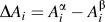
 $${{\partial {\mu _i}} \over {\partial t}} = {D_{ij}}{\nabla ^2}{\mu _j} - \Delta {A_i}{X_{ii}}h'\left( \varphi \right){{\partial \varphi } \over {\partial t}} - {X_{ii}}\left( {{{\partial {\chi _{ii}}} \over {\partial T}}{\mu _i} + {{\partial {{\bar{A}}_i}} \over {\partial T}}} \right){{\partial T} \over {\partial t}}\quad ,$$
where D
ij
denotes the diffusion matrix, and
 $\Delta {A_i} = A_i^\alpha - A_i^\beta$
.
Reference Mushongera, Fleck, Kundin, Wang and Emmerich29
This is a set of coupled diffusion equations, where the moving phase field acts as a source of the diffusion potential since the progressing solid/liquid phase transformation provides a release or an entrapping of chemical elements. The last two terms on the right hand side account for the fact that the thermodynamic parameters A
i
(T) and X
ii
(T) have an implicit temperature dependence. These terms are necessary to maintain the conservation of chemical elements within the framework of a time-dependent temperature field. The imposed time-dependent temperature field is defined as follows
 $$T\left( {{\bf{x}},t} \right) = {T_0} + {\bf{G}} \cdot \left( {{\bf{x}} - {{\bf{v}}_{\rm{p}}}t} \right)\quad ,$$
where G is the constant temperature gradient, T 0 is the constant reference temperature, and v p the constant pulling velocity. Further, we define the cooling rate R as the scalar product of the temperature gradient and the pulling velocity, i.e., R = v p·G. The temperature field in Eq. (11) is required for the simulation of directional solidification, as will be discussed in detail in Sec. II.B.
B. The solidification configuration and scaling
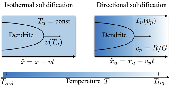
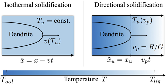
There are two different steady state configurations for solidification available: Isothermal and directional solidification. The dendrite-velocity-undercooling function can be obtained from both configurations, either directly by using isothermal solidification or indirectly via the inverse function using directional solidification, as illustrated in Fig. 1.
Illustration of the relation between the stationary dendritic growth velocity and the tip undercooling temperature within the configuration of (left) isothermal and (right) directional solidification. Isothermal solidification provides the stationary growth velocity as a function of the constant undercooling temperature. Directional solidification provides the stationary tip-undercooling temperature as a function of the imposed pulling velocity. The local temperature is indicated by different shades of blue.
To provide a better control of the numerical stability of the finite-difference solvers and to reduce numerical round-off errors during the calculations, we impose a scaling of the length and times within the simulation. Seeking clarity in the presentation, we introduce the following formalism: To each physical quantity q, we assign a respective scaling constant q 0 as well as a scaled quantity q s = q/q 0, which is used within the simulation. The physical quantity, q, as well as the respective scaling constant, q 0, are both given in the corresponding SI-unit. Unlike the scaled quantity, q s is used in the simulation, which is given in units of the scaling constant q 0. The only exception to this is the temperature, which is treated as an external parameter in our model and is thus not subjected to a scaling. This implies that, for instance, the scaled-temperature gradient is given in units of K/x 0, where K referrers to the SI-unit Kelvin and x 0 referrers to the scaling constant of physical lengths.
The planning of an independent scaling of the lengths by x
0 and the times by t
0 inside the simulation offers the opportunity to set two independent scaling constants. The latter shall be the constant scaling of the energy densities by E
0 and the constant scaling of the diffusion coefficients by D
0. Therefore, we have to identify how the scaling of length x
0 and the scaling of times t
0 relate to the specific choice of E
0 and D
0. The interfacial contribution, ωint, relating to the Gibbs–Thompson effect is given by ωint = ΓV
m/r, where Γ denotes the mean interface energy density with the physical dimension [Γ] = J/m2, V
m denotes the molar volume with the physical dimension [V
m] = m3/mol, and r is the local radius of curvature of the interface with the physical dimension of a length, i.e., [r] = m. From this expression, it is obvious that the Gibbs–Thompson effect involves a coupling of the scaling of the energetics to that of the lengths. Since the chemical energy density contribution in the simulation is scaled by E
0, the interfacial contribution also has to be divided by the same factor to maintain the proper relative energetic weights. Therefore, we can conclude that the scaling constant for the lengths x
0 is calculated as x
0 = V
mΓ0/E
0. Finally, having the length-scale well defined, we can use the diffusion scale D
0 to determine the respective time-scaling via
 ${t_0} = x_0^2{\rm{/}}{D_0}$
.
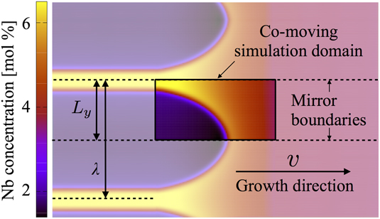
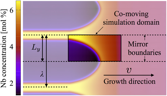
Focusing on stationary states, we describe the steadily proceeding solidification in a co-moving frame of reference. The respective simulation configuration is illustrated in Fig. 2. The simulation domain contains the half of a single solid finger growing at the expense of the surrounding liquid phase along the bottom boundary. To keep the continuously growing solid finger in the center of the simulation domain, we incrementally shift the whole system along the negative x-axes. Whenever the tip of the growing finger exceeds a certain x-position within the simulation domain, an incremental shifting event is performed. This shifting procedure allows a quite efficient simulation of stationary solidification together with the possibility to also access physically meaningful transients between different stationary system states. Conceptually, the domain-shifting-procedure also provides the perspective of growth in an infinitely extended channel, as illustrated by means of the dashed lines in Fig. 2. At the channel walls—i.e., the top and bottom boundary of the simulation domain—no-flux boundary conditions are applied to the phase-field as well as the multiple diffusion potential fields. Therefore, we obtain an effective mirroring of the physical system at these boundary planes. The respective symmetric extension of the system results in a periodic array of symmetric fingers, with a tip spacing λ given by the double of the channel width L y, as also illustrated in Fig. 2. At the important in-flux boundary in front of the growing finger, we aim to impose a completely liquefied system at a chemical state, which corresponds to the original alloying composition of the considered alloy. Therefore, we have to impose respective temperature-dependent constant values for the chemical diffusion potentials there. Those values can be computed with the formula for the nonequilibrium concentration in the liquid phase as written in the text below Eq. (9).
Illustration of the simulation configuration: A single half dendritic finger is growing in the channel indicated by the dashed lines. Mirror boundary conditions (i.e., no-flux) are imposed at the channel walls. The system is frequently shifted such that the growing dendritic finger always remains in the center of the simulation domain, as indicated by the rectangular box with full color. The symmetric extension of the single half dendritic finger to the periodic array of symmetric dendritic fingers is illustrated by the light coloring in the background. The coloring denotes the local Nb concentration, as given by the color bar on the left side of the figure.
III. SIMULATION OF SOLIDIFICATION IN INCONEL 718
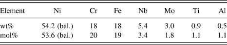
The imposed alloying composition of Inconel 718 is listed in Table I. Based on this composition, CALPHAD calculation using the commercial software-package ThermoCalc in conjunction with the thermodynamic and kinetic databases TTNi8 and MobNi1 have been performed.
28
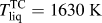
More specifically, within a total temperature range from 1700 K down to 1400 K, only the solid fcc-matrix phase and the liquid phase have been considered. Starting from high temperature, at first, the liquid phase is the only equilibrium phase. This single-phase equilibrium zone ends at the liquids temperature of
 $T_{{\rm{liq}}}^{{\rm{TC}}} = 1630\;{\rm{K}}$
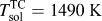
. Then the solid/liquid two-phase equilibrium range is followed until the solidus temperature of
 $T_{{\rm{sol}}}^{{\rm{TC}}} = 1490\;{\rm{K}}$
. Below that temperature, only the solid fcc-matrix phase is stable. It is quite interesting to compare the CALPHAD prediction for the solidification window of Inconel 718 with the respective experimental findings: With the above mentioned values, the ThermoCalc predicts a solidification window of
 $T_{{\rm{liq}}}^{{\rm{TC}}} - T_{{\rm{sol}}}^{{\rm{TC}}} = 140\;{\rm{K}}$
. In contrast to this, experimental solidus
 $\left( {T_{{\rm{sol}}}^{\exp } = 1528\;{\rm{K}}} \right)$
and liquidus temperatures
 $\hbox( {T_{{\rm{liq}}}^{\exp } = 1610\;{\rm{K}}} \hbox)$
found for Inconel 718
Reference Pottlacher, Hosaeus, Wilthan, Kaschnitz and Seifter38
lead to a solidification window of
 $T_{{\rm{liq}}}^{\exp } - T_{{\rm{sol}}}^{\exp } = 82\;{\rm{K}}$
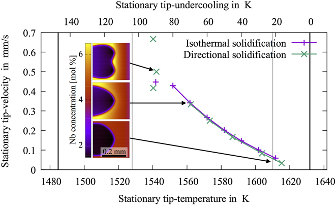
, which is nearly half of that predicted by ThermoCalc. This substantial discrepancy is also visualized in Fig. 5 by the two black and the two gray vertical lines indicating, respectively, the CALPHAD prediction and experimental temperatures. We point out that this discrepancy does not relate to the small variations in the different chemical compositions of the different variants of Inconel 718. Performing the same CALPHAD calculation using exactly the same Inconel 718 variant, as was used in the experiment,
Reference Pottlacher, Hosaeus, Wilthan, Kaschnitz and Seifter38
still provides a solidification window of about 137 K, which is only marginally better. The discrepancy is related to the details of how the material-system is represented within the thermodynamic database. Switching to alternative thermodynamic databases, such as the TCNiX database, make these results look very different. Nevertheless, here the simulations have been based on the thermodynamic input data received from ThermoCalc and are in conjunction with the thermodynamic database TTNi8.
Alloy composition used in the simulations.

A. 1D simulations of solidification
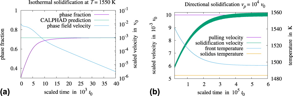
First, we consider the chemically diffusion limited solidification at a constant undercooling temperature in a fixed and one-dimensional (1D) simulation domain. During the simulation, we employ the constant temperature T = 1550 K, which is in-between the above mentioned solidus and liquidus temperatures received form ThermoCalc. The equilibrium matrix phase fraction at this temperature is about 0.72. More specifically, we consider a 1D system, which consists of the liquid phase with a small solid-phase fraction on the left hand side and homogeneous concentrations according to the composition of the Inconel 718 alloy (see Table I). During the course of the simulation, the respective two-phase equilibrium state develops out. Finally, the solidification terminates, when the thermodynamic phase fraction is reached, as can be seen in Fig. 3(a). In conjunction with the solid-phase fraction, the concentrations evolve toward the respective equilibrium distributions.
Plots of the evolution of simulation-measures, such as the solid-phase fraction, the front velocity, and the front temperature, during the course of the one-dimensional simulation of (a) isothermal and (b) directional solidification. The thermo-kinetic parameters used in this simulation study have been generated with. 28 Other parameters are shown in Table II. The velocity is scaled by v 0 = x 0/t 0.
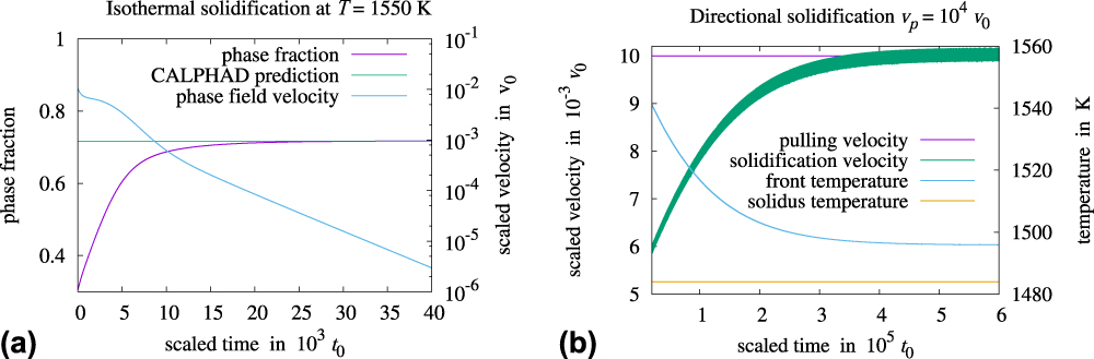
In case of directional solidification, as plotted in Fig. 3(b), it can be seen that upon reaching the steady state both the solidification front velocity as well as the solidification front temperature converge to a constant value. The solidification velocity converges nicely to the imposed pulling velocity, as required by energetic considerations. However, the tip-temperature fails to converge to the expectation value, which is T sol of Inconel 718, by about 25 K. This deviation from the physical expectation is not serious. It can be explained by the fact that the chosen pulling velocity is too high to allow the stationary growth of the planar solidification front in the infinite system. Instead, we have obtained a stationary solution in a finite system, which is tied to the finite length in the x-direction. Due to this, the total alloying composition also deviates from the original composition of Inconel 718.
B. Determination of the scaling constants
The scaling parameters used for the solidification simulation are listed in Table II. For each parameter, we also provide the equation on how the respective parameter relates to the others. The way how the scaling parameters are systematically found one after other, i.e., from the top line to the bottom-line in Table II, is described in detail in the following.
Summary of the imposed parameters for the simulation of dendritic solidification in Inconel 718.

We start with the first four lines in the table, i.e., the required literature data of the material. That is the temperature-dependent mass density, the molar mass, the, respectively, calculated molar volume as well as the interfacial energy density of the solid/liquid interface. The last of these quantities is the one which is most difficult to determine. In fact, it was not possible to directly find a value for the mean interfacial energy density for Inconel 718. Instead, we found the quite reliable value for pure Nickel of ΓNi = 0.3 J/m2. Reference Bragard, Karma, Lee and Plapp10,Reference Nestler, Danilov and Galenko39
The next step in the determination of the scaling of the solidification simulation is to find proper values for the diffusion scaling constant D 0 as well as the energy scale E 0. These two scales are required to ensure the numerical stability of the explicit finite-difference-schemes, with which the multicomponent diffusion equation as well as the phase-field equation is solved. For the determination of these, we have run respective 1D test-simulations, such as the one described above in Sec. III.A. Generally, it should be the aim to find the slowest possible (i.e., still numerically stable) energy scaling constant E 0 and the largest possible diffusion scaling constant D 0. Physically, for such 1D test-simulations with planar fronts, the proper energetic weighting of the Gibbs–Thompson-effect is not important. Nevertheless, also for 1D simulations, the choice of the mean interfacial energy density is not completely arbitrary. Also in this case, the interfacial energy needs to be large enough in comparison to the driving force to ensure sufficient phase stability or in other words to avoid the unphysical nucleation of the thermodynamically favored phase.
Then, we have to define an appropriate length scale x
0 for the simulation. This length scale has to be extracted from the experimental or physical system, which the simulation aims to reproduce. For the present purpose, this shall be the primary dendrite arm spacing found in single crystalline-casted Inconel 718 samples, i.e., λ = 0.3 mm. As listed in line seven of Table II, we have set the scaled channel width
 $L_{\rm{y}}^{\rm{s}}$
to
 $L_{\rm{y}}^{\rm{s}} = 50{x_0}$
. Therefore, the scaling constant for the lengths x
0 is given by the ratio of the experimental arm spacing λ and the respective correspondence in the simulation, i.e., x
0=3 μm. After that, we can calculate the scaling constant for the time using the diffusion scale D
0 and the previously determined length scale x
0.
Finally, we calculate the scaling constant of the mean interfacial energy Γ0, based on the knowledge of E 0, x 0, and V m. Knowing the interfacial energy scale is necessary to calculate the scaled interfacial energy Γs, which has to be imposed in the simulation. It turns out that the scaled mean interfacial energy has to be chosen quite small, i.e., Γs = 8 × 10⁻⁶Γ0, to reflect the difference in the energetics between the thermodynamic and the Gibbs–Thompson effect properly. We point out that, within the present phase-field formulation, it is not possible to impose such a small value for the interfacial energy. Even if numerically well resolved, respective simulations do not exhibit sufficient phase stability. This means that, for instance, the liquid phase at the initial alloying composition could not exist at temperatures below the liquids temperature without an immediate nucleation of the solid phase. This spuriously enhanced nucleation of the solid phase is fundamentally related to the fact that the solid/liquid interface needs to be chosen orders of magnitude wider than it’s actual physical width. With the necessity to have an unrealistically wide solid/liquid interface, the respective amount of total physical interface energy is also distributed over that too large area. Therefore, it can no longer be sufficient to act as a nucleation barrier against the other stronger driving forces.
However, as a consequence of this, the very small Gibbs–Thompson effect needs to be overestimated in a systematic and controlled way. The performance of such a systematic overestimation of the Gibbs–Thompson effect should be conceptually related to what is done in the framework of the above-mentioned thin interface asymptotic analysis. However, within this article, no such systematic approach has been applied. Here, we impose a scaled mean interfacial energy of
 ${\tilde{\Gamma }^{\rm{s}}} = 0.2{\Gamma _0}$
instead of Γs = 8 × 10⁻⁶Γ0, which corresponds to an overestimation of more than four orders of magnitude.
C. 2D simulation of solidification
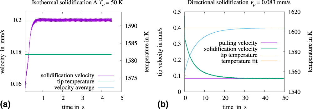
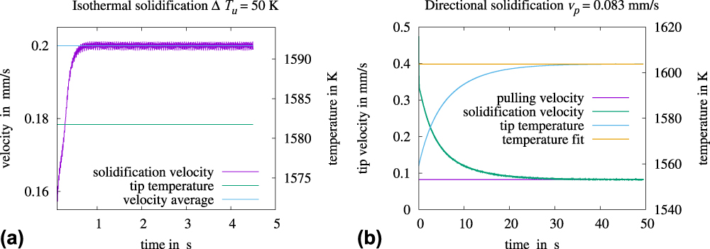
We discuss the steadily proceeding solidification in a co-moving frame of reference. This description is naturally efficient and the resulting steady states of the system are independent from initialization details. The two possible steady state configurations for solidification are the isothermal and the directional solidification. In Fig. 4(a), the time-evolution of the momentary tip velocity in physical units is plotted. After a short transient, the velocity quickly becomes constant within the framework of some small numerical fluctuations, which result from the influence of the numerical grid on the motion of the phase field. If required, the amplitude of these numerical fluctuations can be reduced by increasing the phase field width ξ relative to the distance between numerical lattice grid points. However, the stationary growth velocity is extracted by averaging over the numerically fluctuating velocities, as also indicated in Fig. 4(a). The time evolution of the tip-temperature and the growth velocity during the simulation of 2D directional solidification is shown in Fig. 4(b). Note that these velocities are also subjected to numerical fluctuations.
Plots of the simulation-time evolution of the tip-temperature as well as the tip-velocity during the simulation of (a) isothermal and (b) directional solidification. The thermo-kinetic parameters used in this simulation study have been generated with. 28 The other parameters used in these simulations are listed in Table II.
In Fig. 5, we compare the obtained stationary velocity-temperature function form the simulation of isothermal growth with the inverse relation obtained from the simulations of directional solidification. The results have been plotted within a temperature range, which ranges from the CALPHAD solidus temperature of
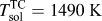 $T_{{\rm{sol}}}^{{\rm{TC}}} = 1490\;{\rm{K}}$
up to the respective liquidus temperature of
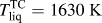 $T_{{\rm{liq}}}^{{\rm{TC}}} = 1630\;{\rm{K}}$
. In Fig. 5, both of these temperatures have been indicated by solid black vertical lines. For the sake of comparison, we also show experimental solidus
 $\left( {T_{{\rm{sol}}}^{\exp } = 1528\;{\rm{K}}} \right)$
and liquidus temperatures
 $\hbox( {T_{{\rm{liq}}}^{\exp } = 1610\;{\rm{K}}} \hbox)$
found for Inconel 718,
Reference Pottlacher, Hosaeus, Wilthan, Kaschnitz and Seifter38
as indicated by the vertical gray lines in Fig. 5. This discrepancy is related to details of how the material system is represented in the underlying thermodynamic database TTNi8. The application of alternative thermodynamic databases may lead to very different results as discussed above. The experimental temperatures, of course, do not have any direct relation to the present simulation study, as these have been based on the thermo-kinetic input data received from ThermoCalc in conjunction with TTNi8. The top axis of the graph contains the undercooling temperature, which vanishes at the liquidus temperature
 $T_{{\rm{liq}}}^{{\rm{TC}}}$
and is inversely related to the usual temperature printed on the bottom axis of the graph.
Comparison of the relation between the stationary dendritic growth velocity as a function of the tip-undercooling temperature, respectively, for isothermal and directional solidification in Inconel 718. The thermo-kinetic parameters used in this simulation study have been generated with. 28 Other parameters are shown in Table II. The color plots in the insets are showing exemplarily three different stationary Nb concentration distributions.

Generally, we observe a very similar solidification behavior for the two different stationary configurations, indicating that the model provides a self-consistent description of solidification in Inconel 718. More specifically, at low undercooling temperatures, we find stationary states where a single cell-like dendritic finger is growing into the liquid phase. Here, for the two different solidification configurations, the model provides quantitative agreement between the respective stationary velocity versus tip-undercooling-temperature relation, as indicated by the interconnected data points in Fig. 5. The interconnection lines shall help to identify the assignment between the data points and the configurations. With regard to the trends of the two different functions, when approaching the zero solidification velocity limit, we obtain temperatures which are only marginally below the liquidus temperature. Of course, without the Gibbs–Thomson effect one would expect to see the growth velocity to vanish exactly at vanishing undercooling temperatures. However, including the effect of the interface energy, first a small nucleation barrier energy given by the Gibbs–Thompson effect has to be overcome so that the growth of a dendrite can start. Then the undercooling temperature of the zero growth velocity limit corresponds to that of the nucleation barrier energy.
For lower temperatures or larger undercoolings, the growth of a single dendritic finger becomes less and less favorable in a channel of a fixed width. As faster growing dendritic fingers take up less space, their fitting into the fixed channel gets increasingly unfavorable, eventually leading to the appearance of a second tip. However, since the boundary conditions imposed at the channel walls rather stabilize the growth of a single half dendritic finger, they, in turn also kind of suppress the convergence to stationary states with two tips. Therefore, at the end of the range of stable single-finger-growth, we do not directly obtain the expected stable two-finger growth but first obtain some nonstationary fluctuations toward this state. These intermediate nonstationary states are indicated as isolated data points in the plot in Fig. 5, where an average tip-undercooling temperature together with the respective average velocity has been taken to quantitatively characterize the respective simulation state. The transition to the nonstationary states happens for directional solidification as well as for free growth at comparable velocities or undercooling temperatures, which again indicates that the model provides a self-consistent description of solidification in Inconel 718.
Finally, we would like to discuss the relation between the obtained simulation results and respective experimental conditions found for the solidification in Inconel 718 during single crystalline casting experiments. In the respective experiments, a pulling velocity of
 $v_{\rm{p}}^{{\rm{exp}}} = 0.05\;{\rm{mm/s}}$
and a temperature gradient of about G
exp ≈ 20 K/mm has been applied. This has resulted in single crystal samples, where a primary dendrite arm spacing of about λexp ≈ 0.3 mm has been observed. As already mentioned above, the length scales in the simulation have been fitted to the experimental primary dendrite arm spacing. Using the respective scaling, as listed in Table II, the imposed temperature gradient in our simulations correspond to a physical temperature gradient of G = 33 K/mm. This is quite close to the temperature gradient used in the single crystalline casting experiments, and simulations using exactly the experimental value could be easily realized within the forthcoming simulation studies, aiming at more quantitative descriptions of the single crystalline solidification in Inconel 718. The experimental pulling velocity of
 $v_{\rm{p}}^{\exp } = 0.05\;{\rm{mm/s}}$
has been reached in the simulations, as shown in Fig. 5.
A quite substantial discrepancy between the present simulation results and respective casting experiments is found with regard to the solidification morphology. The single-crystalline casting samples show the typical dendritic microstructure, which consists of a network of primary, secondary, and sometimes even tertiary dendritic arms, unlike the simulations, where we rather observe a cell-like solidification with just a primary arm and no further side branching. This discrepancy is certainly a result of the heavy overestimation of the interfacial energy density, as discussed above. Further, we would like to point out that the computed velocity versus undercooling relation, given in Fig. 5, is very much tight to the specific choice of our underlying simulation configuration, as illustrated in Fig. 2. In particular, we expect some quantitative disagreement between the relation in Fig. 5 and velocity versus undercooling relations seen in real Bridgman experiments.
IV. CONCLUSION
In this article, we have developed a phase field model for the simulation of chemical diffusion-limited solidification in multicomponent alloys. The model involves a simplified thermodynamic description, where the two relevant phases, solid and liquid, are both modeled as solution-phases with a finite solubility range and parabolic thermodynamic potential energy densities. The temperature-dependent thermo-kinetic parameters, required in the model, are generated on the basis of the CALPHAD solid/liquid two-phase equilibrium. More specifically, temperature-dependent equilibrium concentrations of phases, Gibbs free energies of phases, chemical diffusion potentials of the thermodynamic factor matrix as well as the diffusion matrix have been generated using the commercial CALPHAD software-package ThermoCalc in conjunction with the thermodynamic and kinetic databases TTNi8 and MobNi1. 28 The temperature-dependent model-parameters related to the parabolic thermodynamic description can be derived from this set of thermodynamic information according to Eqs. (7) and (8). To obtain a well-defined dendritic selection, we consider the solid/liquid interface in our model to be anisotropic with respect to the interfacial energy as well as with regard to the transformation kinetics. The anisotropy strength of the two interfacial properties can be chosen independent from each other in our model.
The implementation of the model allows us to consider the proceeding solidification in a co-moving simulation domain, which follows the continuously growing dendritic tip. The focus has been on the analysis of stationary solidification states, i.e., the dendrite is growing with a constant velocity, and the shape of the solid/liquid interface becomes time independent within the co-moving frame of reference. As illustrated in Fig. 1, two different well-defined stationary configurations have been considered: The isothermal as well as the directional solidification. During the isothermal solidification, we impose a spatially constant and time-independent undercooling temperature below the liquidus temperature of the alloy. This constant undercooling temperature drives the solidification, resulting in a certain growth velocity of the dendrite tip. In contrast to this, during directional solidification, the constant solidification velocity is imposed via the time-dependent linear gradient temperature field. As a result, the stationary dendrite tip-undercooling temperature is selected during the solidification.
The model has been applied to the simulation of solidification in Inconel 718, which is defined via the alloying composition in Table I. Employing this composition, we have generated the temperature-dependent thermo-kinetic input data using the ThermoCalc as well as the DICTRA-module of the ThermoCalc software system in conjunction with the thermodynamic and kinetic databases TTNi8 and MobNi1. 28 To find proper scaling constants for the energetics E 0 and kinetics D 0, which guaranty a stable numerical operation, 1-dimensional solidification simulations have been performed. In Fig. 3(a), we compare the results of the two different solidification configurations: Isothermal and directional solidification. Based on the two scaling constants E 0 and D 0, a proper scaling of the length and time within the simulation has been setup. The respective scaling parameters used in the two-dimensional simulation studies are listed in Table II.
However, it turned out that a straight forward scaling of the solidification with a physically correct weighting of the thermodynamic energetics and the interface energy has not been possible using the present formulation. More specifically, the mean interfacial energy density, i.e., the Gibbs–Thompson effect, has been overestimated by more than four orders of magnitude to ensure sufficient phase stability and to avoid spuriously enhanced solid-phase nucleation.
Then, two dimensional simulation studies of isothermal and directional solidification have been performed. In Fig. 5, we compare the two, respectively, obtained stationary velocity-undercooling functions. For stationary diffusion limited growth of a single dendritic finger, we find a good agreement between the two respective functions, which indicates that the model provides a self-consistent description of the solidification even in the presence of time-dependent linear gradient temperature fields.
Finally, we compare the obtained simulation results with experimental conditions found for the solidification in Inconel 718 during single crystalline casting experiments. In the respective experiments, a pulling velocity of
 $v_{\rm{p}}^{\exp } = 0.05\;{\rm{mm/s}}$
and a temperature gradient of about G
exp ≈ 20 K/mm has been applied. This has resulted in single crystal samples, where a primary dendrite arm spacing of about λexp ≈ 0.3 mm has been observed. Substantial discrepancies between the simulation results and respective casting experiments in Inconel 718 are found with regard to the solidification morphology. While the single-crystalline casting samples show the typical dendritic side-branching, in the simulations, we observe a cell-like solidification morphology without side-branching. This discrepancy is mainly a result of the heavy overestimation of the interfacial energy density.
ACKNOWLEDGMENTS
We thank the Federal Ministry for Economics and Energy (BMWi) of the Federal Republic of Germany for the financial support under the running project COORETEC: ISar (funding code: 03ET7047D) Further, we thank the Federal Ministry of Education and Research (BMBF) for the financial support under the running project ParaPhase (funding code: 01IH15005B). Furthermore, parts of the research presented in this article have received funding from the European Union’s Seventh Framework Program (FP7/2007-2013) for the Clean Sky Joint Technology Initiative under grant agreement number 326020. Also, we thank the MTU Aero Engines AG for the fruit-full collaboration within the research project SIMCHAIN. Finally, we thank the German Research Foundation (DFG) for the financial support within the second phase of the priority program 1713.