INTRODUCTION
Alpine glacial meltwater is utilized by many human populations for potable water, agriculture, and hydroelectric power (e.g., Milner et al., Reference Milner, Khamis, Battin, Brittain, Barrand, Füreder and Cauvy-Fraunié2017). Such environments are especially vulnerable to natural and anthropogenic environmental changes due to limited acid-neutralizing capacities, thick seasonal snow-cover, short growing seasons, thin soils, relatively low bedrock chemical weathering rates, and large volumes of snowmelt generated in the spring (Campbell et al., Reference Campbell, Clow, Ingersoll, Mast, Spahr and Turk1995). Because alpine and subalpine ecosystems have well-defined hydrobiogeochemical boundaries, they are suited for applications of robust research techniques and proxies that allow for quantification of mass fluxes across subsystem boundaries (e.g., Campbell et al., Reference Campbell, Clow, Ingersoll, Mast, Spahr and Turk1995; Beniston, Reference Beniston2003; MacGregor et al., Reference MacGregor, Riihimaki, Myrbo, Shapley and Jankowski2011; Moser et al., Reference Moser, Baron, Brahney, Oleksy, Saros, Hundey and Sadro2019; Burpee and Saros, Reference Burpee and Saros2020). Lakes exhibit naturally well-defined basin margins and are the low points of a landscape. Consequently, even open lacustrine systems lend themselves to studies of cross-boundary elemental transfers by integrating environmental processes operating within their watersheds and within the lake basin itself. Lake sediments archive natural temporal climatic, hydrological, and biogeochemical changes that occurred in the geological past (e.g., Catalan et al., Reference Catalan, Pla-Rabés, Wolfe, Smol, Rühland, Anderson and Kopáček2013; Moser et al., Reference Moser, Baron, Brahney, Oleksy, Saros, Hundey and Sadro2019).
The North American Rocky Mountains contain a major [sub]alpine lake district, and similar districts occur globally (Burpee and Saros, Reference Burpee and Saros2020). The Loch Vale watershed (LVW) with its outlet lake, The Loch, is located within this district in Rocky Mountain National Park, Colorado USA (Fig. 1). The LVW is a small, glaciated, monitored watershed with extensive hydrological, meteorological, and stream-water chemical data dating back to 1982 (e.g., Baron, Reference Baron and Baron1992a).
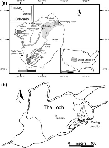
Locality and site information for The Loch and Loch Vale watershed (LVW): (a) Location and geographic features of the LVW shown within the USA (lower right inset), Colorado (upper left inset), and within Rocky Mountain National Park (RMNP). Glaciers indicated by striped fill. (b) Bathymetry of The Loch in meters including coring location (after Baron, Reference Baron and Baron1992b). ACW = Andrews Creek Watershed.

Despite its location in a high-elevation remote wilderness, The Loch has been experiencing increases in algal biomass since ca. 1950 (Wolfe et al., Reference Wolfe, Van Gorp and Baron2003; Elser et al., Reference Elser, Andersen, Baron, Bergström, Jansson, Kyle, Nydick, Steger and Hessen2009; Oleksy et al., Reference Oleksy, Baron, Leavitt and Spaulding2020). These algal blooms are attributed to increases in anthropogenic reactive nitrogen (N) deposition along the Colorado Front Range (e.g., Mast et al., Reference Mast, Clow, Baron and Wetherbee2014; Oleksy et al., Reference Oleksy, Baron, Leavitt and Spaulding2020). As with N, phosphorus (P5+, often reported as orthophosphate PO43−) may contribute to algal blooms (e.g., Bostrom and Petterson, Reference Bostrom and Petterson1982; Smith et al., Reference Smith, Tilman and Nekola1999; Baken et al., Reference Baken, Moens, van der Grift and Smolders2016; Krumina et al., Reference Krumina, Kenney, Loring and Persson2016). The bedrock within the LVW contains the mineral apatite (Ca5(PO4)3(OH,F,Cl)), and is dissolving sufficiently rapidly to have released PO43− at a flux of ~50 mol ha−1 year−1 from 1984–2008 (Price et al., Reference Price, Peresolak, Brice and Tefend2013, 2020). This value is ~20× greater than the global average reported from models by Hartmann et al. (Reference Hartmann, Moosdorf, Lauerwald, Hinderer and West2014). Despite such a high lithogenic PO43− flux within the LVW from 1982–2018, <1% of stream outlet samples had P5+ concentrations ([P5+]) above the maximum reported detection limit of 0.307 mg L−1 (data from https://www2.nrel.colostate.edu/projects/lvws; accessed June 10, 2020) where detections limits have varied temporally.
The cycling of P5+ is a complex interaction among water, sediment, and aquatic biota. Phosphorus also plays a critical role in global climate due to the relationship between atmospheric carbon dioxide and marine photosynthetic productivity (e.g., Broecker, Reference Broecker1982). However, relatively little is known about P5+ behavior in glaciated watersheds and associated lakes (e.g., Hodson et al., Reference Hodson, Mumford and Lister2004, Reference Hodson, Mumford, Kohler and Wynn2005; Ren et al., Reference Ren, Martyniuk, Oleksy, Swain and Hotaling2019). Investigating present-day P5+ subsidies and sources is very challenging both in the LVW and elsewhere, and exacerbated by P5+ being monoisotopic. Neodymium (Nd) isotopic ratios (143Nd/144Nd) have been argued to fingerprint P5+ sources (e.g., Arvin et al., Reference Arvin, Riebe, Aciego and Blakowski2017) because Nd, among other rare earth elements (REEs), is commonly found in phosphate minerals (Chadwick et al., Reference Chadwick, Derry, Vitousek, Huebert and Hedin1999). However, within the LVW, Price et al. (Reference Price, Moore and Kerans2017) demonstrated that the REEs (data from Shiller, Reference Shiller2010) are derived from bedrock monazite dissolution, which only contributes ~0.1% of the P5+ to weathering solutions. The remaining ~99.9% of P5+ is derived from primary apatite dissolution, and consequently for the LVW, the mineralogic source of the REEs is not the primary P5+ producer. Rare earth elements also may be sourced from highly soluble silicate minerals such as allanite (e.g., Price et al., Reference Price, Velbel and Patino2005, Reference Price, Wilton, Tubrett, Schneiderman, Fan and Peresolak2014). These observations seriously call into question the validity of indiscriminately using REE isotopes as P5+ tracers.
The LVW is an ideal location to study P5+ behavior because it is known to have high lithogenic P5+ fluxes to lakes and streams (Price et al., Reference Price, Nunez and Moore2020). The ~50 mol P5+ ha−1 year−1 from LVW bedrock is approximately an order of magnitude higher than measured atmospheric combined wet and dry deposition P5+ fluxes from the Colorado Front Range (Baron and Denning, Reference Baron, Denning and Baron1992; Baron et al., Reference Baron, Denning, McLaughlin and Baron1992a; Mladenov et al., Reference Mladenov, Williams, Schmidt and Cawley2012; Heindel et al., Reference Heindel, Putman, Murphy, Repert and Hinckley2020), and two orders of magnitude higher than atmospheric dry-deposition P5+ fluxes alone (Oldani et al., Reference Oldani, Mladenov, Williams, Campbell and Lipson2017). Atmospheric dry-deposition P5+ fluxes should be treated as maximum values because aeolian phosphate mineral solubility is currently poorly understood (Brahney et al., Reference Brahney, Ballantyne, Kociolek, Spaulding, Otu, Porwoll and Neff2014; Price et al., Reference Price, Nunez and Moore2020). In addition, multidecadal climatic, hydrologic, and biogeochemical data are available for the LVW.
Lacustrine sediment cores have been collected from The Loch and analyzed for [P5+] to investigate natural temporal changes through geologic time (Price et al., Reference Price, Moore and Kerans2017). These lake-bottom sediments record the timing of glacial retreat from the end of the Pinedale glaciation through the Early Holocene, a time represented by the largest and most-punctuated climatic variability in the last 100,000 years (Lora and Ibarra, Reference Lora and Ibarra2019; Quirk et al., Reference Quirk, Mackey, Fernandez, Armstrong and Moore2020). Therefore, with so few [PO43−] measurements above detection limits in present-day outlet-stream waters, The Loch sediments preserve a dateable record of changes in [P5+] that occurred during relatively rapid, large-amplitude paleoclimatic oscillations that operated during the Pleistocene–Holocene transition. Because diatoms (Bacillariophyceae) can be used in paleolimnological records as indicators of nutrient fluctuations (McKnight et al., Reference McKnight, Smith, Bradbury, Baron and Spaulding1990; Battarbee et al., Reference Battarbee, Anderson, Jeppesen and Leavitt2005; Saros et al., Reference Saros, Michel, Interlandi and Wolfe2005; Slemmons et al., Reference Slemmons, Rodgers, Stone and Saros2017), they are also included in this study. Such biogeochemical data helps to illuminate past and current P5+ behavior, and what to expect as climate changes within the LVW and elsewhere.
METHODS
Site description
The northeast-facing 660 ha subalpine to alpine LVW (Fig. 1) is part of the U.S. Geological Survey's Water, Energy, and Biogeochemical Budgets program (Turk et al., Reference Turk, Spahr and Campbell1993; Lins, Reference Lins1994). Located along the Colorado Front Range in Rocky Mountain National Park, the watershed ranges in elevation from 3050 m above sea level (asl) at the outlet, to 4009 m asl at Taylor Peak on the Continental Divide. During the 1992–2018 period, precipitation in the watershed averaged 109 cm yr−1 (data from https://www2.nrel.colostate.edu/projects/lvws; accessed June 10, 2020) and the annual temperature was 1.4°C (Akie et al., Reference Akie, McDermott, Sexstone and Clow2020). Over 70% of precipitation occurred as snow, with discharge peaking in June during spring melting and negligible during the winter months.
The LVW was affected by Pleistocene and Holocene valley glacial advances, with the highest elevations remaining unglaciated (Madole, Reference Madole and Mahaney1976; Baron and Mast, Reference Baron, Mast and Baron1992). Only 18% of the LVW is vegetated (Arthur, Reference Arthur and Baron1992), 6% is forest, and the remainder is bare rock and talus (Arthur and Fahey, Reference Arthur and Fahey1990; Mast et al., Reference Mast, Drever and Baron1990; Arthur, Reference Arthur and Baron1992). Forests occur on the thickest soils, which are ~56-cm thick, with granite and gneiss till as parent material (Walthall, Reference Walthall1985; Arthur, Reference Arthur and Baron1992; Baron et al., Reference Baron, Walthall, Mast, Arthur and Baron1992b). Above the ~3350 m asl tree line, the alpine tundra vegetation consists of low, mat-like plants. An Engelmann spruce-subalpine fir forest occurs below tree line, grading into lodgepole pine stands below ~3000 m asl (Wardle, Reference Wardle1968; Arthur, Reference Arthur and Baron1992).
Approximately 80% of the LVW bedrock is a 1.8 Ga metasedimentary biotite gneiss, and the remaining bedrock is composed of the intrusive 1.5 Ga Silver Plume granite (Peterman et al., Reference Peterman, Hedge and Braddock1968; Cole, Reference Cole1977; Nesse, Reference Nesse1977; Braddock and Cole, Reference Braddock and Cole1990; Mast, Reference Mast and Baron1992). The mineralogy and chemistry of the two units is nearly identical, with quartz, plagioclase (oligoclase An27), microcline, and biotite as major minerals (Cole, Reference Cole1977; Mast et al., Reference Mast, Drever and Baron1990; Mast, Reference Mast and Baron1992). Magnetite, ilmenite, garnet, epidote, apatite, monazite, zircon, orthopyroxene, calcite, and pyrite occur as minor minerals (Cole, Reference Cole1977; Mast et al., Reference Mast, Drever and Baron1990; Mast, Reference Mast and Baron1992; Price et al., Reference Price, Peresolak, Brice and Tefend2013, Reference Price, Moore and Kerans2017, Reference Price, Nunez and Moore2020).
The Loch is located at 3110 m asl below tree line at the watershed outlet, has the largest surface area of the LVW lakes at 4.98 ha, and a maximum depth of 4.7 m (Fig. 1; Baron, Reference Baron and Baron1992b). It is a Late Pleistocene cirque lake with its basin having formed from valley glacier excavation during Pinedale advances of the Taylor and Andrews glaciers (Fig. 1). Water temperatures in The Loch reach a maximum of 12°C in late summer, with no thermal stratification during the open-water season and inverse thermal stratification when ice-covered (Baron, Reference Baron and Baron1992b). Bathymetric data reveal the deepest portion of The Loch is in the southeast corner (Fig. 1b; Baron, Reference Baron and Baron1992b). The lake-bottom sediments are homogeneous gyttja with no sedimentary varves, laminations, or stratification visible in a split core (Price et al., Reference Price, Moore and Kerans2017). Sediment enters The Loch via Icy Brook (Fig. 1).
Frost-cracking modeling
The frost-cracking modeling used herein is based on one-dimensional heat conduction in rock (Anderson, Reference Anderson1998; see also Hales and Roering, Reference Hales and Roering2007; Savi et al., Reference Savi, Delunel and Schlunegger2015):

where T(z,t) = temperature (°C) as a function of depth (z) in bedrock and time (t), MAT = mean annual temperature (°C), Ta = half the amplitude of the sinusoidal variation (half the difference between maximum summer and winter minimum temperatures in °C), Py = period of one year, and α = thermal diffusivity of rock (1–2 mm2 s−1 from Anderson (Reference Anderson1998); midrange of 1300 cm2 day−1 used in this study). Equation (1) is used to calculate T(z,t) daily for a year. Although the original one-dimensional heat-conduction-in-rock model of Anderson (Reference Anderson1998) has increased in sophistication (Anderson et al., Reference Anderson, Anderson and Tucker2013), the simplicity of Equation (1) works very well for the purposes of this study.
The frost-cracking intensity (FCI; formalized in Eq. 1–6 below) is the annual sum of the temperature gradient (|∂T/∂z|) that occurs in the frost-cracking window of 0°C to −15°C (Girard et al., Reference Girard, Gruber, Weber and Beutel2013; Rempel et al., Reference Rempel, Marshall and Roering2016). A frost-cracking window of −3°C to −8°C is often used based on laboratory experiments performed by Hallet et al. (Reference Hallet, Walder and Stubbs1991) on sandstone. We prefer the 0°C to −15°C window of Girard et al. (Reference Girard, Gruber, Weber and Beutel2013) because it is based on in situ measurements of transient elastic waves in crystalline rock. Therefore,

with i = depth index consisting of whole numbers ranging from 0 to ∞, z ranging from 0 cm to the depth zmax below which $\vert {\partial T/\partial z} \vert = 0{\rm ^{{\circ}}C}{\rm c}{\rm m}^{{-}1}$ for each day (t) during Py, and

which is an important parameter because the larger the Δz, the lower the calculated FCI. Furthermore,

Also,

where,

Specifically, this study had zmax = 1600 cm and Δz = 10 cm, yielding n = 159. For intersite comparisons of the FCI, the Δz values must be equal. For example, doubling the Δz of this study to 20 cm halves the calculated FCI value.
The FCI was calculated for the 1992–2018 period using the most robust meteorological data available (Akie et al., Reference Akie, McDermott, Sexstone and Clow2020). Because winter temperature will influence hydrogeochemical processes throughout the following year, the frost-cracking year used in this study was December to November.
Coring and recovery of lake-bottom sediment
The Loch was chosen for sediment collection because it permits direct comparison with watershed-scale stream chemical-flux values measured at its outlet (Price et al., Reference Price, Moore and Kerans2017). Lake-bottom sediment was collected using percussion-coring equipment fabricated in-house that followed the design of Reasoner (Reference Reasoner1993). Two cores were collected within 1 m of each other on March 8, 2016, through ~1 m-thick lake ice (Fig. 1b); one core was taken for radiocarbon dating and geochemical analyses (Core #2), and the other core was taken to be used for diatom identification (Core #3). Because of their proximity to each other, cores #2 and #3 may be treated as being identical with respect to geochronology and accumulation rate. The two cores were assigned their respective numbers because an earlier core collected from The Loch (i.e., Core #1) was consumed as a result of the studies conducted by and reported on by Price et al. (Reference Price, Moore and Kerans2017). Each continuous core was ~2 m in length and collected near the deepest part of The Loch (Fig. 1b; 40.2925°N, −105.6558°W) at a water depth of ~4.7 m. The deepest part of The Loch was chosen as it likely contains the thickest sediment with optimal conditions for preservation of the oldest material. The cores were cut into three sections in the field, Zorbitrol® was added to any void space (Tomkins et al., Reference Tomkins, Antoniades, Lamoureux and Vincent2007), then the cores were packaged in the field and placed on ice in a cooler for transport. Core #2 was split longitudinally and subdivided into 2 cm intervals (n = 101) at Illinois College, and Core #3 was subdivided into 0.5 cm intervals (n = 390) at the University of Wisconsin-Stevens Point.
Price et al. (Reference Price, Moore and Kerans2017) determined that the sediment of The Loch is dominated by homogeneous gyttja containing over 80% silt with the exception of the basal diamicton below 195 cm. The homogeneity of silt-dominated material from The Loch is important because any up-core geochemical trends cannot be granulometric.
14C dating and age-depth modeling
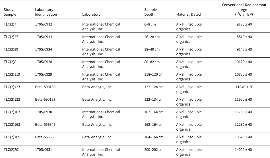
Eleven radiocarbon ages were obtained for Core #2 by accelerator mass spectrometry at International Chemical Analysis, Inc. and Beta Analytic, Inc., located in Miami, Florida (Table 1). Alkali insoluble organic material in the sediments had to be dated due to an absence of terrestrial macrofossils. However, 11 radiocarbon ages from terrestrial macrofossils were obtained for Core #1 (Price et al., Reference Price, Moore and Kerans2017) that yielded organic matter content trends consistent with those of Core #2.
Accelerator mass spectrometry (AMS) ages for the core collected from The Loch.

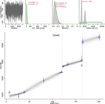
Age-depth modeling was performed using Bacon v. 2.3.9.1, which utilizes Bayesian statistics in the R statistical software environment (Blaauw and Christen, Reference Blaauw and Christen2011). In such Bayesian models, the age uncertainty typically increases with distance from the known ages. R-Bacon combines radiocarbon ages with prior knowledge (“priors”) of sediment accumulation rate, and the extent that the accumulation rate of a particular depth in a core depends on the depth immediately above (“memory”). The core is subdivided into many vertical sections as specified by the user, and through millions of Markov chain Monte Carlo iterations, estimates are created for the accumulation rates of each section. An advantage of R-Bacon is that dates are input as conventional radiocarbon ages (14C BP), with R-Bacon utilizing the IntCal13 database (Reimer et al., Reference Reimer, Bard, Bayliss, Beck, Blackwell, Bronk Ramsey and Buck2013) with calibration being dynamically included in the modeling iterations (Lacourse and Gajewski, Reference Lacourse and Gajewski2020). Using Student's t-test, the age-depth modeling process is robust against outlying dates. R-Bacon was run numerous times using different priors, with the model chosen that exhibited the most stationary iteration distribution and comparability between modeled and input priors. In the final R-Bacon model iteration, the 202-cm core was subdivided into 49 sections, each 4-cm thick, and unconformities added at the 121 cm and 164 cm depths to account for abrupt drops in radiocarbon ages (Table 1).
Sediment phosphorus chemistry
Five different forms of P5+ in the sediment of Core #2 were sequentially extracted following the Standards, Measurements, and Testing Program of the European Commission (SMT method; Ruban et al., Reference Ruban, López-Sánchez, Pardo, Rauret, Muntau and Quevauviller1999a, b, 2001), which is a standardization of phosphorus extraction methods (Wang et al., Reference Wang, Zhang, Li and Morrison2013). The SMT method was subjected to an interlaboratory study for evaluation of the techniques and yielded very favorable and consistent results (Ruban et al., Reference Ruban, López-Sánchez, Pardo, Rauret, Muntau and Quevauviller1999a). The five phosphorus fractions are: 1) Fe-, Al-, and Mn-oxide-bound phosphorus (NP) (adsorbed and authigenic phosphates; Selig et al., Reference Selig, Fischer and Leipe2005); 2) calcium-bound phosphorus such as apatite (HP); 3) total inorganic phosphorus (IP); 4) organic phosphorus (OP); and 5) total phosphorus (TP) (e.g., Ruban et al., Reference Ruban, López-Sánchez, Pardo, Rauret, Muntau and Quevauviller1999a, Reference Ruban, Brigault, Demare and Philippeb, Reference Ruban, López-Sánchez, Pardo, Rauret, Muntau and Quevauviller2001; Huang et al., Reference Huang, Wang, Wang, Wang and Jin2005; Wang et al., Reference Wang, Zhang, Li and Morrison2013). The NP fraction was extracted by initially adding 20 mL of 1 M NaOH to ~200 mg of dry sediment (16 hours), followed by adding 4 mL of 3.5 M HCl to 10 mL of the supernatant (16 hours). Following settling of a brown precipitate, NP was measured in the supernatant. The “N” in “NP” stands for the NaOH used in the initial step. The HP fraction was extracted using the solid residue of the 1 M NaOH solution from the first step of the NP procedure. Following a 1 M NaCl wash of this fraction, 20 mL of 1 M HCl was added (16 hours), and HP measured in the supernatant. The “H” in “HP” stands for the 1 M HCl reagent used in this extraction. The IP fraction was extracted by adding 20 mL of 1 M HCl to ~200 mg of dry sediment (16 hours), and IP measured in the supernatant. The OP fraction was extracted by adding 20 mL of 1 M HCl to the solid residue of the IP fraction following destruction of the organic matter (16 hours), and OP measured in the supernatant. The TP fraction was extracted by adding 20 mL of 3.5 M HCl to ~200 mg of dry sample in which organic matter had been destroyed (16 hours), and TP measured in the supernatant. The IP and TP are determined independently, with IP being comprised of HP and NP, and TP being comprised of HP, NP, and OP (Ruban et al., Reference Ruban, Brigault, Demare and Philippe1999b).
Laboratory analyses of the sequential leachates for phosphorus were performed at Bentley University using a Thermo Scientific iCAP 6300 Duo View inductively coupled plasma optical emission spectrometer and a CETAC ASX-520 autosampler. External calibration curves were generated with single-element standards (High-Purity Standards, Charleston, SC, USA), using deionized water from a Milli-Q Direct 16 system and Optima HNO3. Error on the analyses was determined to be 8% based on multiple analyses of a NIST phosphorus standard.
The NP concentration, CNP, of P in mg g−1 of dry sediment (modified from Ruban et al., Reference Ruban, López-Sánchez, Pardo, Rauret, Muntau and Quevauviller1999a) is given by:

where CE = P concentration in the extract in mg L−1, V = volume of reagent used for extraction (20 mL), and msed = dry mass of sediment used in extract (~200 mg). Similarly, the concentrations of the other four phosphorus fractions, CxP, in mg g−1 of dry sediment (modified from Ruban et al., Reference Ruban, López-Sánchez, Pardo, Rauret, Muntau and Quevauviller1999a) is given by:

Diatom enumeration
Diatom assemblages were identified in every 0.5-cm interval throughout Core #3. Sediment for diatom analysis was treated with 10% HCl to remove carbonate material, followed by 30% H2O2 to remove organic matter. Standard protocols (Battarbee, Reference Battarbee and Berglund1986) were used to prepare diatom slides that were examined under oil immersion at 1000× magnification using a Leica DM2000 LED microscope with differential interference contrast. A minimum of 300 diatom valves were identified and enumerated from random transects from each slide. Diatoms were identified using Krammer and Lange-Bertalot (Reference Krammer, Lange-Bertalot, Ettl, Gerloff, Heynig and Mollenhauer1986, Reference Krammer, Lange-Bertalot, Ettl, Gerloff, Heynig and Mollenhauer1988, Reference Krammer, Lange-Bertalot, Ettl, Gerloff, Heynig and Mollenhauer1991a, Reference Krammer, Lange-Bertalot, Ettl, Gärtner, Gerloff, Heynig and Mollenhauerb), Camburn and Charles (Reference Camburn and Charles2000), and updated to modern taxonomic nomenclature using the Diatoms of the North America website (Spaulding et al., Reference Spaulding, Potapova, Bishop, Lee, Gasperak, Jovanoska, Furey and Edlund2022) and AlgaeBase (Guiry and Guiry, Reference Guiry and Guiry2017). Tychoplanktic and meroplanktic species were classified in the planktic component of the assemblage, and comparisons were conducted to determine if exclusion of species yielded similar patterns.
A weighted-average calibration model was used to determine diatom-inferred total phosphorus (TP) following methods outlined by Juggins and Birks (Reference Juggins, Birks, Birks, Lotter, Juggins and Smol2012). This model assumes that the abundance of a species is greater when conditions are optimal for its growth, with species TP optima being derived from published calibrations sets (Chen et al., Reference Chen, Dalton, Leira and Taylor2008; Cumming et al., Reference Cumming, Laird, Gregory-Eaves, Simpson, Sokal, Nordin and Walker2015). Given the limitations of published TP optima for certain species, only species that comprised the top 10% of the core at any given time were incorporated in the TP-inferred model. No TP optima for Gomphonema brebissonii have been published, so the TP optima was derived from a morphological and ecologically similar species, Gomphonema acuminatum. Care should be taken in the utility of the TP transfer function because the relationship between TP and the relative abundance of diatom taxa can be confounded due to variables such as lake depth, where TP is not the main driver of diatom distribution and abundance, or both (Juggins et al., Reference Juggins, Anderson, Ramstack Hobbs and Heathcote2013).
RESULTS
Frost-cracking modeling
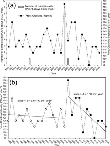
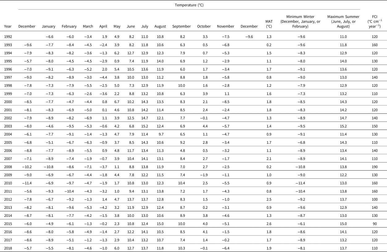
The temperature data and calculated FCI values are provided in Table 2, and FCI values displayed graphically in Figure 2. Table 2 also provides the mean monthly and annual temperature data for the LVW, with the minimum winter (December, January, and February) and maximum summer (June, July, and August) temperatures that were used in the frost-cracking calculations. The highest FCI for the 1992–2018 period was for 2008 at 190°C cm−1 year−1, which was well above the next highest FCI of 160°C cm−1 year−1 calculated for frost-cracking years 1993, 2010, and 2011 (Fig. 2, Table 2).
Plots of (a) number of outlet stream water samples with [PO43−] above the maximum detection limit of 0.307 mg L−1 and frost-cracking intensity (FCI) for the Loch Vale watershed sample period 1992–2018 with the frost-cracking year being December to November, and (b) regression lines for the FCI for 1992–2007 and 2008–2018, with slopes ± uncertainty at 95% confidence plotted.

Monthly and annual temperature data (Akie et al., Reference Akie, McDermott, Sexstone and Clow2020) and frost-cracking intensity calculations for the Loch Vale watershed for the measurement period 1992–2018. Frost-cracking years are December to November, except for 1992 where temperature data for December 1991 is incomplete. MAT = mean annual temperature; FCI = frost-cracking intensity.

Within the uncertainty of the trend slope (−0.4 ± 0.4°C cm−1 year−2 at 95% confidence), there is no statistically significant change in the FCI temporal trend between 1992 and 2007 (Fig. 2b). However, between 2008 and 2018, the FCI temporal trend displays a rapid decline (slope of −6 ± 1°C cm−1 year−2 at 95% confidence), indicating significant climatic warming during that time. Even if the elevated 2008 FCI value is eliminated and the data are limited to between 2009 and 2018, there is still statistically significant climate warming during that time, with the FCI temporal trend exhibiting a slope of −4 ± 1°C cm−1 year−2 at 95% confidence. Noteworthy is that the FCI calculations herein reveal a statistically significant increase in temperature that is not recognizable through climate data alone.
14C dating and age-depth modeling
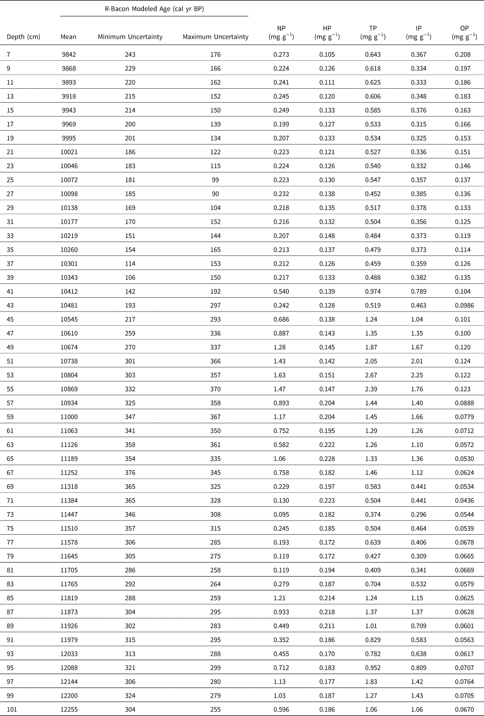
From the radiocarbon ages (Fig. 3, Tables 1, 3), the top surfaces of the sediment cores are modern unconformities. Because the uppermost sample selected for radiocarbon dating was 6–8 cm depth (TLC(2)7), no data are reported or interpreted above that level. From the R-Bacon age-depth model, the base of Core #2 (TLC(2)201) had a mean age of 17,086 calibrated years BP (cal yr BP), with minimum and maximum uncertainty ages at 95% confidence of 16,763 cal yr BP and 17,528 cal yr BP, respectively (Table 3). This age span reflects the initial post-Last Glacial Maximum retreat of Taylor and Andrews glaciers to an elevation exposing The Loch. The uppermost dated sample TLC(2)7 had a mean age of 9,842 cal yr BP, with minimum and maximum uncertainty ages at 95% confidence of 9,599 cal yr BP and 10,018 cal yr BP, respectively (Table 3). Therefore, within uncertainty, Cores #2 and #3 span from the Oldest Dryas stade to the Early Holocene. Although there can be relatively large uncertainties for late-glacial calibrated radiocarbon ages, two depositional hiatuses have been invoked between 16,465 ± 510 cal yr BP and 14,213 ± 204 cal yr BP, and between 13,443 ± 121 cal yr BP and 12,765 ± 89 cal yr BP (Fig. 3, Table 3).
Age-depth model generated using Bacon v. 2.3.9.1 (Blaauw and Christen, Reference Blaauw and Christen2011) with priors and unconformities at 121 cm-depth and 164 cm-depth shown. Note the stationary distribution among neighboring iterations (upper left), and strong similarities between priors and modelled values of accumulation rate (upper two, middle). Gray dashed line reflects error envelope at 95% confidence.

R-Bacon modeled ages with uncertainty at 95% confidence and unconformities at 121 cm-depth and 164 cm-depth, and phosphorus analyses (mg per gram of sediment sample) with 8% uncertainty. NP = Fe-, Al-, and Mn-oxide-bound phosphorus; HP = calcium-bound phosphorus such as apatite; TP = total phosphorus; IP = inorganic phosphorus; OP = organic phosphorus.

Sediment phosphorus chemistry
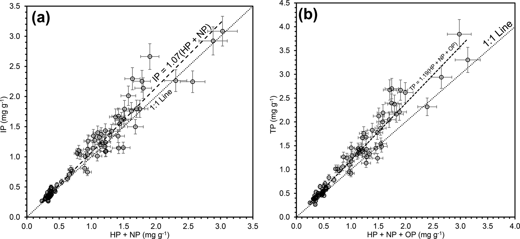
The [P5+] in the sediment for all five fractions is provided in Table 3. Because the IP and TP fractions are processed independently, the following relationships should be maintained, and thus serve as a check on data quality (Ruban et al., Reference Ruban, López-Sánchez, Pardo, Rauret, Muntau and Quevauviller1999a):

and

The data displaying these relationships is provided graphically in Figure 4. The difference between the slopes of the predicted 1:1 line and the actual data reflecting the three P5+ forms in Equation (9) in Figure 4a is 7%, which is within the analytical error of 8%. The larger difference between the slopes of the predicted 1:1 line and the actual data reflecting the four P5+ forms in Equation (10) in Figure 4b is larger at 19%, but includes an additional P5+ form.
Comparison of measured and calculated phosphorus forms from a sediment core recovered from The Loch: (a) IP = HP + NP; (b) TP = HP + NP + OP. Note that with respect to the plot of IP = HP + NP in (a), the difference in slope between the data and the 1:1 line at 7% is less than the analytical error of 8% utilized in this study. IP is inorganic phosphorus, HP is calcium-bound phosphorus, NP is oxide-bound phosphorus, TP is total phosphorus, OP is organic phosphorus.

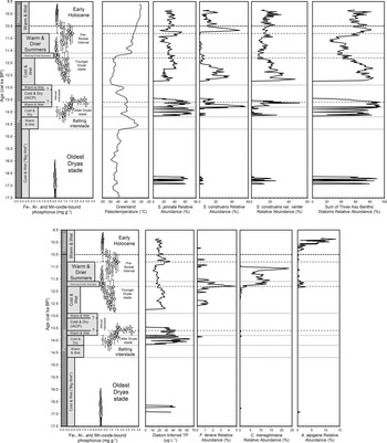
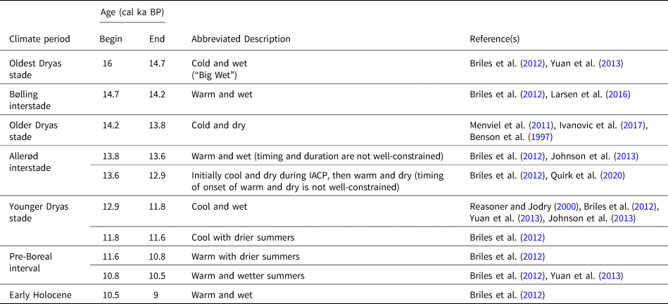
The NP concentrations in the sediment core represent the aqueous dissolved phase in the geologic past with temporal changes in Core #2 shown in Figure 5. For purposes of comparison, Greenland Ice Sheet Project II (GISP2) ice-core temperature data (Alley, Reference Alley2000, Reference Alley2004) are also provided in Figure 5. Numerous studies have demonstrated transmission of North Atlantic paleoclimatic oscillations to western North America (e.g., Phillips et al., Reference Phillips, Zreda, Benson, Plummer, Elmore and Sharma1996; Oviatt, Reference Oviatt1997; Zic et al., Reference Zic, Negrini and Wigand2002; Quirk et al., Reference Quirk, Mackey, Fernandez, Armstrong and Moore2020). The climatic periods, abbreviated descriptions, and ages in Figure 5 are summarized with applicable references in Table 4. It is interesting to note in Figure 5 that many NP changes approximate climatic period boundaries.
Late glacial–interglacial transition summary diagrams for (top row, from left): Fe-, Al-, and Mn-oxide-bound phosphorus (NP), Greenland ice-core temperature (Alley Reference Alley2000, Reference Alley2004), and relative abundances of key benthic diatom taxa including their sum; and (bottom row from left) NP concentrations and paleoclimate trends from top row repeated for clarity, diatom-inferred TP reconstructions, and relative abundances of key planktic diatom taxa for sediment cores collected from The Loch, Colorado, USA. Diatom species: Staurosirella pinnata, Staurosira construens, Staurosira construens var. venter, Fragilaria tenera, Cyclotella meneghiniana, Aulacoseira alpigena.

Southern Rocky Mountain climate periods, ages, abbreviated descriptions, and relevant references for the climatic events identified for this study. Cool and dry climate for the Intra-Allerød Cold Period (IACP) from Quirk et al. (Reference Quirk, Mackey, Fernandez, Armstrong and Moore2020) and for the Wasatch Mountains located ~500 km west of the LVW.

Diatom enumeration
A total of 59 diatom species were identified from Core #3. The 13 species that comprised at least 10% or more of the diatom assemblage at some point in time throughout the core are provided in Supplementary Table 1. This paper focuses only the relative abundance of six key ecologically relevant taxa, including three benthic diatoms, Staurosirella pinnata, Staurosira construens, and Staurosira construens var. venter, with relatively high phosphorus optima (15.1 μg L−1, 13.6 μg L−1, and 14.9 μg L−1, respectively; Cumming et al., Reference Cumming, Laird, Gregory-Eaves, Simpson, Sokal, Nordin and Walker2015). A calibration set from 251 lakes from British Columbia indicate that these three taxa are more abundant in meso-eutrophic conditions where phosphorus levels are above 5 μg L−1 (Cumming et al., Reference Cumming, Laird, Gregory-Eaves, Simpson, Sokal, Nordin and Walker2015). Three planktic diatom taxa, Fragilaria tenera, Aulacoseira alpigena, and Cyclotella meneghiniana, are indicators of increasing lake level and/or elevated nutrients.
The three benthic diatoms, Staurosirella pinnata, Staurosira construens, and Staurosira construens var. venter, are indicators of elevated phosphorus and approximately follow NP (Fig. 5). After the initial Oldest Dryas stade–Bølling interstade hiatus, these taxa undergo a relative increase in abundance during the Older Dryas stade and Allerød interstade (AI). The sum of these three taxa yields a maximum at ca. 13,600 cal yr BP that correlates with the highest NP values of the sediment (Fig. 5). Following the second AI–Younger Dryas stade (YDS) hiatus, Staurosirella pinnata, Staurosira construens, and Staurosira construens var. venter display an overall decline during the YDS that continues into the Pre-Boreal Interval (PBI). These three taxa then peak during the Late Pre-Boreal and remain approximately stable as dominant taxa in the Early Holocene, a trend very similar to that of NP (Fig. 5). This trend is further emphasized by the diatom-inferred TP reconstructions (Supplementary Table 2) that display a peak at ca. 10,800 cal yr BP when NP values also peak (Fig. 5).
The occurrence of Fragilaria tenera, a nitrogen-indicating taxa, increased significantly in relative abundance during the Late YDS between ca. 11,900 cal yr BP and ca. 11,600 cal yr BP (Fig. 5). An increase in the relative abundance of the planktic taxa Cyclotella meneghinia immediately followed the appearance of F. tenera, with elevated C. meneghinia populations persisting until the Late PBI at approximately 11,000 cal yr BP. The taxa Aulacoseira alpigena is the only planktic taxa present during the Early Holocene (Fig. 5).
DISCUSSION
Present-day frost-cracking in bedrock weathering and phosphorus release
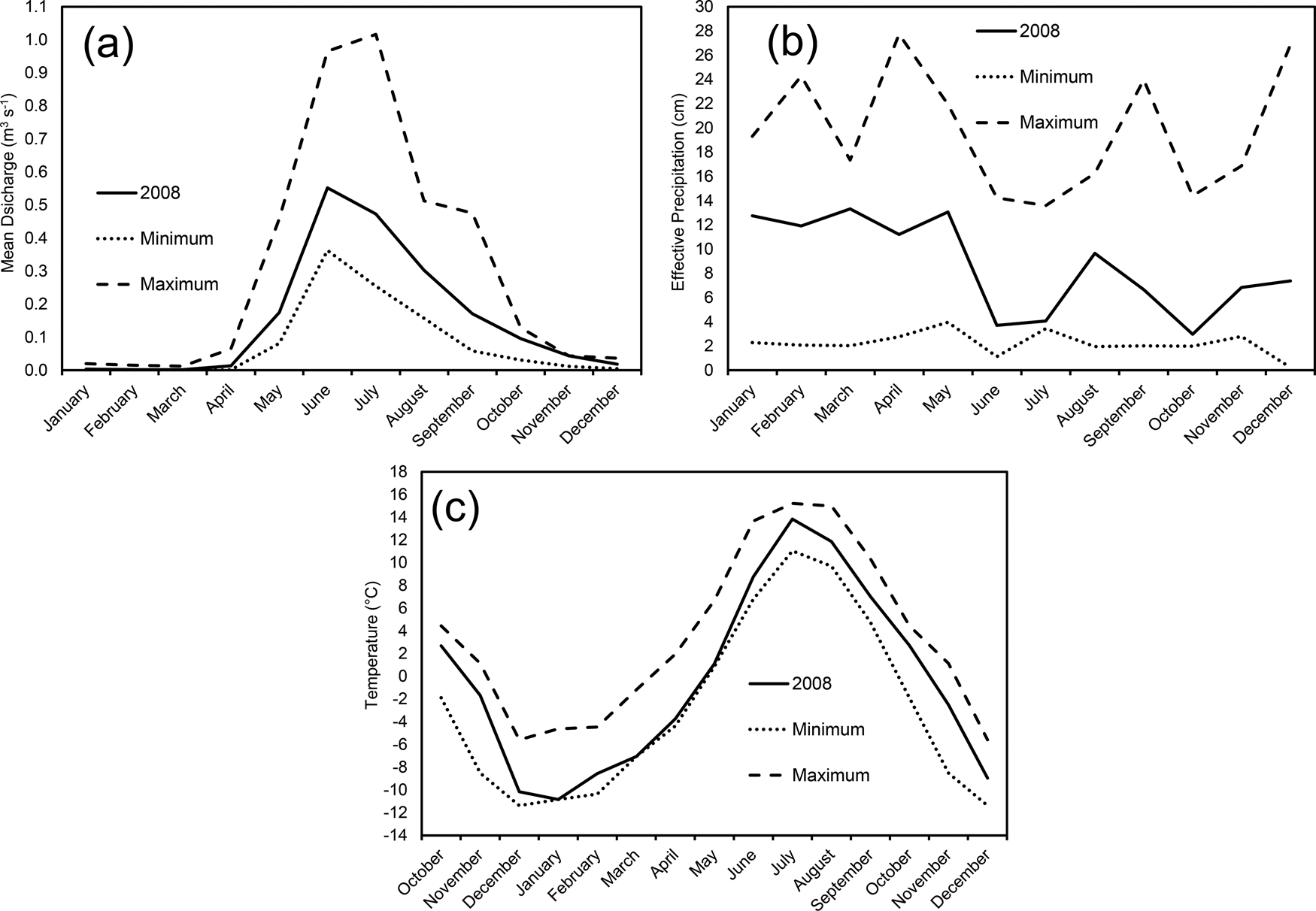
For the sample period 1992–2018, <1% of filtered samples had [PO43−] above the reported maximum detection limit of 0.307 mg L−1 (data from https://www2.nrel.colostate.edu/projects/lvws; accessed June 10, 2020). With nine stream [PO43−] values above the detection limit, 2008 is well above 1998 and 2009, which have one sample each above the detection limit (Fig. 2). Meteorological and hydrologic data for the LVW during 2007–2008 do not reveal any anomalous trends with respect to mean discharge (Fig. 6a) or effective precipitation (Fig. 6b). However, for the 1992–2018 measurement period, January 2008 was the coldest recorded January, July 2008 was relatively warm, and 2008 tied with 1993 for the lowest MAT at 0.2°C (Fig. 6c, Table 2). These observations indicate that a relatively cold winter followed by a relatively warm summer and low MAT increases bedrock apatite dissolution and P5+ release, consistent with the frost-cracking calculations (Equations 1–6). The highest FCI of the period of study being from 2008 is interpreted to indicate that the greater frost-cracking resulted in exposure of highly soluble bedrock apatite grains to weathering agents (see also Price et al., Reference Price, Nunez and Moore2020). This is also consistent with the highest [PO43−] concentrations within the LVW being highest at the Sky Pond inlet (Fig. 1; Baron, Reference Baron and Baron1992b). Therefore, as a first approximation, relatively cold winters followed by relatively warm summers, and a relatively low MAT may increase [PO43−] in stream waters. After the 2008 FCI of 190°C cm−1 year−1, the next-highest FCI of 160 °C cm−1 year−1 occurred in 1993, 2010, and 2011, with none of these years having any detectable [PO43−] in stream waters (Fig. 2b, Table 2). Such a trend may indicate that relatively intense and/or deep frost-cracking above an FCI of 160°C cm−1 year−1 is necessary to expose soluble apatite grains when surficial bedrock is already relatively depleted in apatite following repeated years of less-intense frost-cracking.
Plots of (a) minimum and maximum monthly stream discharge, (b) effective precipitation, and (c) temperature for the Loch Vale watershed for 1992–2018, and 2008 monthly measures for comparison. Temperature data includes October, November, and December data from previous year to provide complete winter data for preceding year. Stream discharge and precipitation data taken from https://www2.nrel.colostate.edu/projects/lvws [accessed June 10, 2020 ] and temperature from Akie et al. (Reference Akie, McDermott, Sexstone and Clow2020).

Paleoclimatic controls on phosphorus concentrations in sediments of The Loch
Cold climates with increased frost-cracking would enhance apatite dissolution and associated P5+ release to ground and surface waters. Because NP is the adsorbed P5+ fraction in sediments, enhanced apatite dissolution should be reflected as elevated NP in sediments deposited on the bottom of The Loch (Fig. 1). Increases in NP associated with colder temperatures are consistent with the maximum NP observed in Core #2 during the AI, including during the Intra-Allerød Cold Period (IACP; Fig. 5). Despite cooling during the YDS, NP concentrations in sediments of The Loch display an overall declining trend during the YDS (Fig. 5). Therefore, the relationship between [P5+] and climate is more complicated than that predicted from frost-cracking alone.
Previous laboratory studies of sediment collected from anthropogenically affected [meso]eutrophic lakes have argued that P5+ may migrate to surface sediments post-depositionally (e.g., Carignan and Flett, Reference Carignan and Flett1981; Rydin, Reference Rydin2000; Ostrofsky, Reference Ostrofsky2012). Such studies contend that following deposition under anoxic conditions to depths within ~15 cm, P5+ migrates upwards over periods of days or weeks, and reprecipitates as ferric and manganic hydroxides in the oxic top 1–2 cm of the sediments. We do not believe that such diagenetic redox-driven P5+ migration is an issue for the The Loch sediments investigated in this study. The Loch has experienced relatively steady and low sediment deposition rates of ~0.5 mm year−1 (Fig. 3, Table 3), which is significantly slower than the rate of redox-driven P5+ diffusion upward in the sediment column. As sediment deposition progressed in The Loch, the ~15-cm-thick redox-sensitive surface zone would have continued to move upwards. The sediments below the ~15 cm-deep redox boundary would be relatively depleted in P5+ and display homogenization or up-core monotonic increases in P5+, with any significant temporal fluctuations in NP likely being lost. In contrast, NP concentrations in sediment recovered from The Loch display temporal variability as dramatic as and correlative with climate fluctuations during the Pleistocene–Holocene transition (Fig. 5). Furthermore, the highest NP concentrations at ca. 13,600 cal yr BP correlate with the highest relative abundance sum for the P5+-indicating diatoms Staurosirella pinnata, Staurosira construens, and Staurosira construens var. venter (Fig. 5). The other lesser NP peak at ca. 10,800 cal yr BP correlates with a diatom-inferred TP reconstruction peak (Fig. 5). Thus, the diatom data provide strong evidence that redox-driven P5+ migration has not been significant for lake-bottom sediments of The Loch.
The NP concentrations at the base of Core #2 during the cold Oldest Dryas Stadial are extremely low (Fig. 5). The diatoms Staurosirella pinnata, Staurosira construens, and Staurosira construens var. venter, indicators of elevated phosphorus (Cumming et al., Reference Cumming, Laird, Gregory-Eaves, Simpson, Sokal, Nordin and Walker2015), are the dominant taxa and appear intermittently during this time (Fig. 5). The Oldest Dryas stade is also termed the “Big Wet” (Yuan et al., Reference Yuan, Koran and Valdez2013; Fig. 5, Table 4), with the relatively low NP observed during the Oldest Dryas stade likely reflecting dilution from increased rainfall and/or cryospheric melting. An extremely high stream discharge associated with increased rainfall and/or cryospheric melting is likely responsible for the unconformity present from the Late Oldest Dryas Stadial and through the entire warm and wet Bølling interstade (Fig. 5).
The end of this initial depositional hiatus in Core #2 approximately corresponds with the beginning of the Older Dryas stade at ca. 14,200 cal yr BP (Table 4). This boundary likely reflects the end of Pinedale alpine glacial retreat following the last glacial maximum (Fig. 5). The NP values increase rapidly during the Older Dryas stade and into the AI, a climatic period dominated by cold and dry conditions for the southern Rocky Mountains (Benson et al., Reference Benson, Burdett, Lund, Kashgarin and Mensing1997; Menviel et al., Reference Menviel, Timmerman, Timm and Mouchet2011; Briles et al., Reference Briles, Whitlock and Meltzer2012; Ivanovic et al., Reference Ivanovic, Gregoire, Wickert, Valdes and Burke2017; Quirk et al., Reference Quirk, Mackey, Fernandez, Armstrong and Moore2020). Although a relatively minor warm and wet period has been reported for the Early AI, its timing is not well constrained. The GISP2 ice core temperature data (Alley, Reference Alley2000, Reference Alley2004) indicate an overall cooling trend for the North Atlantic during the AI (Fig. 5), with the IACP centered on ca. 13,200 cal yr BP. Several of the samples with the highest NP concentrations in Core #2 occur during the IACP. Radiocarbon dates specifically on the samples with the highest NP concentrations (Tables 1, 3) yields a robust correlation with the IACP. This provides evidence that the abrupt North Atlantic cooling of the IACP was transmitted to the LVW and created conditions that were dry with relatively cold winters, warm summers, and a relatively low MAT. Quirk et al. (Reference Quirk, Mackey, Fernandez, Armstrong and Moore2020) had a similar finding from δ18O data for a speleothem from the Wasatch Mountains of the eastern Great Basin, USA, located ~500 km west of the LVW. Furthermore, Sapota et al. (Reference Sapota, Aldahan and Al-Aasm2006) found vivianite, an iron phosphate mineral (Fe3(PO4)2⋅8H2O) indicative of elevated aqueous phosphorus concentrations, in Siberian Lake Baikal sediments that was deposited during the climatologically cold and dry post-Miocene. The unconformity in the core occurring in the Late AI may indicate that sufficiently cold conditions created stream discharge that was too low for lacustrine sediment deposition during that time.
The decline in NP at the beginning of the YDS reflects the transition to wetter winters, springs, and summers in the southern Rocky Mountains (Briles et al., Reference Briles, Whitlock and Meltzer2012; Yuan et al., Reference Yuan, Koran and Valdez2013). Summer temperatures cooled by ~0.4–0.9C° and alpine glaciers advanced in the LVW (Reasoner and Jodry, Reference Reasoner and Jodry2000) and elsewhere in Colorado (Johnson et al., Reference Johnson, Jiménez-Moreno, Eppes, Diemer and Stone2013). While the cooler temperatures would have enhanced frost-cracking, the increased precipitation would have had a diluting effect on [P5+]. Hence, NP values are intermediate during the mid-YDS before further declining in response to wetter conditions as YDS glaciers receded during the warmer and dryer YDS–PBI transition (Briles et al., Reference Briles, Whitlock and Meltzer2012; Yuan et al., Reference Yuan, Koran and Valdez2013; Fig. 5). The relative abundance of the planktic diatom taxa Fragilaria tenera increased during the Late YDS (Fig. 5), and is a robust indicator of increased nitrogen concentrations in The Loch, consistent with present-day glacial melting within the LVW (Baron et al., Reference Baron, Schmidt and Hartman2009; Heath and Baron, Reference Heath and Baron2014) and elsewhere (Saros et al., Reference Saros, Rose, Clow, Stephens, Nurse, Arnett, Stone, Williamson and Wolfe2010; Slemmons and Saros, Reference Slemmons and Saros2012; Slemmons et al., Reference Slemmons, Saros and Simon2013, Reference Slemmons, Saros, Stone, McGowan, Hess and Cahl2015). Glacial melting at the end of the YDS is consistent with Menounos and Reasoner (Reference Menounos and Reasoner1997) for the LVW, and resulted in wetter conditions and reduced lacustrine [P5+].
The planktic diatom taxa Cyclotella meneghiniana indicates shallow, nutrient-rich littoral waters, appears in Late YDS, and peaks in relative abundance in the middle PBI (Fig. 5). During this time in The Loch, NP concentrations monotonically rise (Fig. 5). The increase in NP is consistent with a shallow, nutrient-rich lake resulting from a warmer climate with drier summers, together yielding enhanced evaporation in the southern Rocky Mountains (Briles et al., Reference Briles, Whitlock and Meltzer2012; Table 4). At ca. 10,800 cal yr BP, climate changes to warm with wetter summers in the southern Rocky Mountains in response to an increasing North American Monsoon (Briles et al., Reference Briles, Whitlock and Meltzer2012; Yuan et al., Reference Yuan, Koran and Valdez2013; Table 4). This climate transition follows shortly after the loss of Cyclotella meneghiniana and is consistent with the onset of steadily declining NP and a spike in Staurosirella pinnata (Fig. 5). These wetter summers were accompanied by a steady decline in NP to the Pleistocene–Holocene boundary at ca. 10,500 cal yr BP for the LVW (Price et al., Reference Price, Moore and Kerans2017), at which point, NP concentrations remain approximately constant to the unconformable top of the core. This steady NP behavior likely reflects the onset of stable, warm and wet climatic conditions that characterize the Holocene.
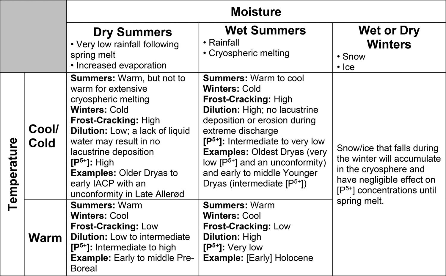
Figure 7 provides a matrix summarizing the climatic effects on [P5+] in alpine to subalpine lakes as presented above. Relatively cold winters followed by relatively warm summers, and a relatively low MAT optimize the frost-cracking of bedrock and exposure of highly reactive apatite to weathering agents. Dry climatic conditions minimize dilution of aqueous P5+. Consequently, at one extreme, a cold and dry climate is optimum for elevated [P5+] which occurred during the Older Dryas Stadial and into the IACP (Figs. 5, 7). At the other extreme, the lowest [P5+] occur during warm climates with wet summers, such as that during Early Holocene.
Matrix of climatic conditions and their influence on [P5+] in a glaciated watershed. IACP is Intra-Allerød Cold Period.

Implications for climatic controls on lacustrine phosphorus concentrations
Lakes within the LVW are currently experiencing increases in algal biomass (Wolfe et al., Reference Wolfe, Van Gorp and Baron2003; Elser et al., Reference Elser, Andersen, Baron, Bergström, Jansson, Kyle, Nydick, Steger and Hessen2009; Oleksy et al., Reference Oleksy, Baron, Leavitt and Spaulding2020) despite being above 3,050 m asl in the remote alpine to subalpine wilderness of Rocky Mountain National Park, Colorado, USA. The LVW has experienced increases in atmospheric reactive N deposition and substantial ecosystem response since ca. 1950 (Baron et al., Reference Baron, Rueth, Wolfe, Nydick, Alstott, Minear and Moraska2000; Baron, Reference Baron2006; Oleksy et al., Reference Oleksy, Baron, Leavitt and Spaulding2020). However, stream and lake nitrate concentrations have been declining since the mid-2000s in response to reduced anthropogenic NOx emissions (Mast et al., Reference Mast, Clow, Baron and Wetherbee2014). After N, P5+ is the other major nutrient that controls lacustrine algal productivity. Since the late 1990s, increases in summer temperatures have resulted in crysopheric melting and increased discharges in the LVW (Price et al., Reference Price, Peresolak, Brice and Tefend2013; Heath and Baron, Reference Heath and Baron2014). As the results of this study indicate, rapid decreases in FCI have been occurring since 2008, and a warmer climate will reduce frost-cracking. Wetter summers, whether through increased rainfall in any season and/or enhanced melting following a wet winter, will increase dilution of aqueous P5+ in surface waters. The lower [P5+] combined with reductions in nitrate concentrations in The Loch should result in a reduction in algal biovolumes, and potential increased ecosystem reliance on aeolian P5+ deposition (e.g., Brahney et al., Reference Brahney, Ballantyne, Kociolek, Spaulding, Otu, Porwoll and Neff2014) as P-limitation increases. However, the reduction in nitrate concentrations indicates an environmental improvement, whereas crysopheric melting and reductions in the FCI indicate the adverse effects of climate change.
The results of this study show that concentrations of adsorbed elements such as P5+ in lake sediments may have the potential to serve as paleoclimatic proxy data both in the LVW and elsewhere. The LVW exhibits an apatite dissolution rate that yields a P5+ flux that is ~20 times greater than the global average (Price et al., Reference Price, Peresolak, Brice and Tefend2013, Reference Price, Nunez and Moore2020; Hartmann et al., Reference Hartmann, Moosdorf, Lauerwald, Hinderer and West2014). However, even relatively low phosphate mineral weathering rates may yield sufficient detectable P5+ in lacustrine sediments to serve as paleoclimatic proxy data. This would be similar to accessory bedrock monazite dissolution yielding REEs which occurred in very low adsorbed concentrations in sediment from The Loch, but still provided paleoenvironmental proxy data (Price et al., Reference Price, Moore and Kerans2017).
The findings of this study may be extended to lower elevation eutrophic water bodies, including coastal areas, i.e., increases in extreme precipitation events and/or cryospheric melting attributable to climate change have the potential to reduce nutrient concentrations and associated eutrophic effects in surface waters.
CONCLUSIONS
Delineating the controls on [P5+] using present-day surface-water chemistry may be very challenging, if not impossible, because the Late Holocene climate does not offer adequate variability to optimally resolve the influence of climate on [P5+]. Collection and high-resolution analyses of Late Pleistocene to Early Holocene lake sediment cores helped overcome this issue. Fe-, Al-, and Mn-oxide-bound phosphorus (adsorbed and authigenic phosphates; NP) in a lake sediment core from the subalpine lake, The Loch, located along the Colorado Front Range, indicates that optimum conditions for elevated [P5+] are relatively cold winters followed by relatively warm summers, a relatively low mean annual temperature, and minimal rainfall and/or limited summer cryospheric melting. Such climatic conditions enhance frost-cracking and subsequent increased exposure of highly soluble bedrock apatite to weathering agents. Furthermore, calculation of the frost-cracking intensity (FCI) has the potential to illuminate climatic warming that is not statistically resolvable through temperature data alone.
The addition of water to The Loch, through increases in either rainfall or melting of snow, ice, or both, has the potential to dilute [P5+]. Within The Loch, the highest measured NP coincided with the cold and dry Intra-Allerød Cold Period. Measurement of NP in lake sediment cores not only illuminates controls on [P5+] in lacustrine environments, but also has the potential to serve as a paleoclimate proxy. Warming summer temperatures and melting of the permanent cryosphere in the LVW, combined with reductions in frost-cracking mean that The Loch will likely experience future decreases in [P5+]. In response, The Loch may undergo reductions in lacustrine productivity, enhanced ecological P-limitation, and increased reliance on aeolian P5+ deposition. Elsewhere, increases in extreme precipitation events and/or cryospheric melting attributable to a changing global climate may have the potential to reduce anthropogenic eutrophic impacts in surface waters, including those in coastal regions, through nutrient dilution.
Acknowledgments
The authors wish to thank K. Catalano of Bentley University who provided much needed analytical expertise and assistance. J. Langdon and M. Johnson offered helpful insight into mathematical notation. Senior editor D. Booth, associate editor P. Langdon, M. Devey, and an anonymous reviewer all provided thoughtful reviews that greatly enhanced the quality of this manuscript. Logistical support and data were provided by the USGS-supported Loch Vale Watershed Long-term Ecological Research and Monitoring program, and Colorado State University.
Financial Support
This work was supported by the National Science Foundation (grant number OIA-1557417) and Wayne State College Professional Development Funds.
Supplementary Material
The supplementary material for this article can be found at https://doi.org/10.1017/qua.2022.19