1 Introduction
The behaviour of droplets under the action of magnetic fields of different configurations is an important issue in many fields, including microfluidics (Seeman et al. Reference Seeman, Brinkman, Pfohl and Herminghaus2012), mechanics of tissues (Douezan et al. Reference Douezan, Guevorkian, Naouar, Dufour, Cuvelier and Brochard-Wyart2011; Frasca et al. Reference Frasca, Du, Bacri, Gazeau, Gay and Wilhelm2014), studies of dynamic self-assembly (Timonen et al. Reference Timonen, Latikka, Leibler, Ras and Ikkala2013) and many others. After the successful synthesis of magnetic fluids in the late 1960s by Rosensweig (Reference Rosensweig1985), an exciting story about droplets of magnetic fluid began. At first the elongation of the droplets in an external field was observed and explained by Arhipenko, Barkov & Bashtovoi (Reference Arhipenko, Barkov and Bashtovoi1978). The characteristic hysteresis at a sufficiently high magnetic susceptibility of the magnetic fluid was described by Bacri & Salin (Reference Bacri and Salin1982). This problem is quite similar to the deformation of a conducting liquid droplet studied by Taylor (Reference Taylor1964), which also described the so-called Taylor cone and the jet formation from the tip of the droplet. Recently, progress has been made in studying the dynamics of magnetic drop deformation (Rowghanian, Meinhart & Camps Reference Rowghanian, Meinhart and Camps2016).
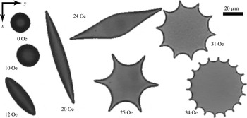
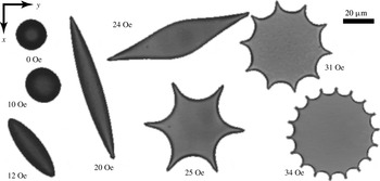
Phase separation of magnetic colloids enabled researchers to obtain magnetic micro-droplets with a very high magnetic susceptibility allowing for the observation of different new phenomena. One particularly interesting case is the behaviour of a magnetic micro-droplet under the action of a rotating magnetic field (Bacri, Cebers & Perzynski Reference Bacri, Cebers and Perzynski1994). At low and intermediate rotating field frequencies, synchronous and asynchronous rotation of the droplet with respect to the rotating field was observed by Sandre et al. (Reference Sandre, Browaeys, Perzynski, Bacri, Cabuil and Rosensweig1999). Depending on the magnetic field strength and frequency, various shapes were seen (Janiaud et al. Reference Janiaud, Elias, Bacri, Cabuil and Perzynski2000). A family of stationary droplet shapes is observed in the present work as shown in figure 1. They are formed under the action of a high-frequency rotating field. A detailed description of the observed sequence of bifurcations is given below.
Stationary shapes of a single magnetic droplet (
 $R_{0}=10~\unicode[STIX]{x03BC}\text{m}$
) in a magnetic field rotating in the
 $(x,y)$
plane at various magnetic field
 $H_{0}$
values. Field frequency is 500 Hz.
In a high-frequency field the characteristic time of the shape deformation is much larger than the field period, therefore it is possible to average the magnetic field energy with respect to the field period. As a result, the droplet shape is a figure of equilibrium and is determined by the balance of the ponderomotive forces of the self-magnetic field and the capillary forces (Bacri et al. Reference Bacri, Cebers and Perzynski1994). On this basis in Bacri et al. (Reference Bacri, Cebers and Perzynski1994), Cebers & Lacis (Reference Cebers and Lacis1995) the re-entrant transition for the sequence of shapes oblate–prolate–oblate was described by applying the virial method and assuming that prolate ellipsoid of revolution arises at the oblate–prolate–oblate bifurcations. Later, these results were extended in Morozov & Lebedev (Reference Morozov and Lebedev2000), Morozov, Engel & Lebedev (Reference Morozov, Engel and Lebedev2002) considering the general ellipsoid with three non-equal axes at the oblate–prolate–oblate bifurcations. An essential assumption of these models is the ellipsoidal shape of the droplet.
Our aim is to answer the following question. Is it possible to describe the set of arising bifurcations by a simple model of a magnetic fluid (Rosensweig Reference Rosensweig1985)? For that, we develop a numerical algorithm for a droplet in a rotating field which is free from the limitations of the ellipsoidal approximation. We compare the numerical results with experimental ones (including those shown in figure 1) and also with analytical results, where possible. We organize the paper as follows. In § 2 we formulate the model and give the available theoretical results. The numerical algorithm is based on a boundary-integral equation technique. It is described with its tests in § 3. The implementation written in the Julia programming language can be found in Erdmanis (Reference Erdmanis2016). In § 4 the numerical analysis of the magnetic droplet shape bifurcations is carried out. The presentation of the experimental results and their comparison with numerical and theoretical results are carried out in § 5, before a short discussion and conclusion.
2 Model and analytical results
2.1 Equation of motion and energy functional
Equations of motion of the magnetic fluid read (Rosensweig Reference Rosensweig1985; Blums, Cebers & Maiorov Reference Blums, Cebers and Maiorov1997)
 $$\begin{eqnarray}-\unicode[STIX]{x1D735}p+\frac{\unicode[STIX]{x2202}\unicode[STIX]{x1D748}_{k}^{v}}{\unicode[STIX]{x2202}x_{k}}+\frac{\unicode[STIX]{x2202}\boldsymbol{T}_{k}}{\unicode[STIX]{x2202}x_{k}}=0;\quad \unicode[STIX]{x1D735}\boldsymbol{\cdot }\boldsymbol{v}=0,\end{eqnarray}$$
where
 $\unicode[STIX]{x1D70E}_{ik}^{v}=\unicode[STIX]{x1D702}(\unicode[STIX]{x2202}v_{i}/\unicode[STIX]{x2202}x_{k}+\unicode[STIX]{x2202}v_{k}/\unicode[STIX]{x2202}x_{i})$
is the viscous stress tensor,
 $\unicode[STIX]{x1D702}$
is the viscosity,
 $p$
is the pressure,
 $\boldsymbol{e}_{i}\boldsymbol{\cdot }\boldsymbol{T}_{k}=1/4\unicode[STIX]{x03C0}(H_{i}B_{k}-1/2H^{2}\unicode[STIX]{x1D6FF}_{ik})$
is the Maxwell stress tensor and
 $\unicode[STIX]{x2202}\boldsymbol{T}_{k}/\unicode[STIX]{x2202}x_{k}=(\boldsymbol{M}\boldsymbol{\cdot }\unicode[STIX]{x1D735})\boldsymbol{H}$
. According to the equations of magnetostatics
 $\unicode[STIX]{x1D735}\boldsymbol{\cdot }\boldsymbol{B}=0;~\boldsymbol{B}=\boldsymbol{H}+4\unicode[STIX]{x03C0}\boldsymbol{M}$
and
 $\unicode[STIX]{x1D735}\times \boldsymbol{H}=4\unicode[STIX]{x03C0}\boldsymbol{J}/c$
(
 $\boldsymbol{J}$
is the current density in external coils creating the magnetic field and equal to zero throughout the volume of the magnetic fluid.). In the framework of the linear response, magnetization
 $\boldsymbol{M}$
expresses as
 $\boldsymbol{M}=\unicode[STIX]{x1D712}\boldsymbol{H}$
, with magnetic susceptibility
 $\unicode[STIX]{x1D712}$
such as
 $\unicode[STIX]{x1D707}=1+4\unicode[STIX]{x03C0}\unicode[STIX]{x1D712}=\text{const.}$
,
 $\unicode[STIX]{x1D707}$
being the magnetic permeability. The equilibrium shapes of the magnetic fluid droplet are usually analysed considering the energy functional (Bacri & Salin Reference Bacri and Salin1982) (see Landau & Lifshitz (Reference Landau and Lifshitz1960) for the derivation of the magnetic field contribution)
 $$\begin{eqnarray}E=-\frac{1}{2}\int \boldsymbol{M}\boldsymbol{\cdot }\boldsymbol{H}_{0}\,\text{d}V+\unicode[STIX]{x1D6FE}S,\end{eqnarray}$$
where
 $\boldsymbol{H}_{0}$
is the field strength of the external homogeneous magnetic field,
 $S$
is the surface area of a droplet and
 $\unicode[STIX]{x1D6FE}$
is the surface tension (supposed here independent of
 $H$
). Although this approach, as should be expected, is reasonable, for the completeness of further analysis we illustrate below that it directly follows from the dynamic equations (2.1) and the boundary conditions describing the evolution of the shapes of the droplet.
Considering the Lagrange variation of some variable
 $f$
(
 $\unicode[STIX]{x1D743}(\boldsymbol{x})$
is the displacement of material element with a radius vector
 $\boldsymbol{x}$
)
 $$\begin{eqnarray}\unicode[STIX]{x1D6FF}_{L}\,f=f^{\prime }(\boldsymbol{x}^{\prime })-f(\boldsymbol{x});\quad \boldsymbol{x}^{\prime }=\boldsymbol{x}+\unicode[STIX]{x1D743}(\boldsymbol{x})\end{eqnarray}$$
and its derivative
 $$\begin{eqnarray}\unicode[STIX]{x1D6FF}_{L}\frac{\unicode[STIX]{x2202}f}{\unicode[STIX]{x2202}x_{i}}=\frac{\unicode[STIX]{x2202}\unicode[STIX]{x1D6FF}_{L}\,f}{\unicode[STIX]{x2202}x_{i}}-\frac{\unicode[STIX]{x2202}\unicode[STIX]{x1D709}_{k}}{\unicode[STIX]{x2202}x_{i}}\frac{\unicode[STIX]{x2202}f}{\unicode[STIX]{x2202}x_{k}},\end{eqnarray}$$
while the current of external source is fixed according to (2.4) we have (
 $\unicode[STIX]{x1D713}$
being the potential of the magnetostatic field defined by
 $\boldsymbol{H}=\unicode[STIX]{x1D735}\unicode[STIX]{x1D713}$
)
 $$\begin{eqnarray}\unicode[STIX]{x1D6FF}_{L}H_{i}=\frac{\unicode[STIX]{x2202}\unicode[STIX]{x1D6FF}_{L}\unicode[STIX]{x1D713}}{\unicode[STIX]{x2202}x_{i}}-H_{k}\frac{\unicode[STIX]{x2202}\unicode[STIX]{x1D709}_{k}}{\unicode[STIX]{x2202}x_{i}}.\end{eqnarray}$$
For simplicity we further assume that the fluid is incompressible (
 $\unicode[STIX]{x1D735}\boldsymbol{\cdot }\unicode[STIX]{x1D743}=0$
). According to (2.5) we have
 $$\begin{eqnarray}\frac{1}{4\unicode[STIX]{x03C0}}B_{i}\unicode[STIX]{x1D6FF}_{L}H_{i}=\frac{1}{4\unicode[STIX]{x03C0}}B_{i}\frac{\unicode[STIX]{x2202}\unicode[STIX]{x1D6FF}_{L}\unicode[STIX]{x1D713}}{\unicode[STIX]{x2202}x_{i}}-\frac{1}{4\unicode[STIX]{x03C0}}H_{i}B_{k}\frac{\unicode[STIX]{x2202}\unicode[STIX]{x1D709}_{i}}{\unicode[STIX]{x2202}x_{k}}.\end{eqnarray}$$
Integrating the relation (2.6) over the entire volume and accounting for the boundary conditions on the surface of a droplet
 $\unicode[STIX]{x1D6FF}_{L}\unicode[STIX]{x1D713}^{i}=\unicode[STIX]{x1D6FF}_{L}\unicode[STIX]{x1D713}^{e}$
and
 $B_{n}^{i}=B_{n}^{e}$
we obtain (by superscripts
 $^{i}$
and
 $^{e}$
we denote the values on the inside and outside boundaries of the droplet respectively)
 $$\begin{eqnarray}\frac{1}{4\unicode[STIX]{x03C0}}\int B_{i}\unicode[STIX]{x1D6FF}_{L}H_{i}\,\text{d}V=\int \unicode[STIX]{x1D709}_{i}\frac{\unicode[STIX]{x2202}}{\unicode[STIX]{x2202}x_{k}}\left(\frac{H_{i}B_{k}}{4\unicode[STIX]{x03C0}}\right)\,\text{d}V-\int \left(\frac{H_{i}^{i}B_{k}^{i}}{4\unicode[STIX]{x03C0}}-\frac{H_{i}^{e}B_{k}^{e}}{4\unicode[STIX]{x03C0}}\right)\unicode[STIX]{x1D709}_{i}n_{k}\,\text{d}S.\end{eqnarray}$$
Taking into account the identity valid for an incompressible fluid
 $$\begin{eqnarray}-\!\int \unicode[STIX]{x1D709}_{i}\frac{\unicode[STIX]{x2202}}{\unicode[STIX]{x2202}x_{k}}\left(\frac{H^{2}}{8\unicode[STIX]{x03C0}}\unicode[STIX]{x1D6FF}_{ik}\right)\text{d}V+\int \unicode[STIX]{x1D709}_{i}n_{k}\left(\frac{(H^{i})^{2}}{8\unicode[STIX]{x03C0}}-\frac{(H^{e})^{2}}{8\unicode[STIX]{x03C0}}\right)\unicode[STIX]{x1D6FF}_{ik}\,\text{d}S=0\end{eqnarray}$$
the relation (2.7) may be rewritten as follows
 $$\begin{eqnarray}\frac{1}{4\unicode[STIX]{x03C0}}\int B_{i}\unicode[STIX]{x1D6FF}_{L}H_{i}\,\text{d}V=\int \unicode[STIX]{x1D709}_{i}\frac{\unicode[STIX]{x2202}T_{ik}}{\unicode[STIX]{x2202}x_{k}}\,\text{d}V-\int \unicode[STIX]{x1D709}_{i}n_{k}(T_{ik}^{i}-T_{ik}^{e})\,\text{d}S.\end{eqnarray}$$
Using
 $\unicode[STIX]{x1D709}_{i}=v_{i}\unicode[STIX]{x1D6FF}t$
, integrating the dot product of (2.1) with the fluid velocity field and accounting for the incompressibility we obtain (
 $\unicode[STIX]{x1D70E}_{ik}=-p\unicode[STIX]{x1D6FF}_{ik}+\unicode[STIX]{x1D70E}_{ik}^{v}$
)
 $$\begin{eqnarray}\int v_{i}(\unicode[STIX]{x1D70E}_{ik}^{i}+T_{ik}^{i}-\unicode[STIX]{x1D70E}_{ik}^{e}-T_{ik}^{e})n_{k}\,\text{d}S+\frac{1}{4\unicode[STIX]{x03C0}}\int \boldsymbol{B}\boldsymbol{\cdot }\frac{\unicode[STIX]{x1D6FF}_{L}\boldsymbol{H}}{\unicode[STIX]{x1D6FF}t}\,\text{d}V-\int \frac{\unicode[STIX]{x2202}v_{i}}{\unicode[STIX]{x2202}x_{k}}\unicode[STIX]{x1D70E}_{ik}^{v}\,\text{d}V=0.\end{eqnarray}$$
The balance of forces on the boundary of the droplet gives
 $$\begin{eqnarray}(\unicode[STIX]{x1D70E}_{ik}^{i}+T_{ik}^{i}-\unicode[STIX]{x1D70E}_{ik}^{e}-T_{ik}^{e})n_{k}=-\unicode[STIX]{x1D6FE}\left(\frac{1}{R_{1}}+\frac{1}{R_{2}}\right)n_{i},\end{eqnarray}$$
where
 $1/R_{1,2}$
are principal curvatures. As a result we conclude that the variation of the sum of the surface energy
 $\unicode[STIX]{x1D6FE}S$
and the thermodynamic potential at fixed current in the external coils
 $\tilde{F}=-1/8\unicode[STIX]{x03C0}\int \boldsymbol{B}\boldsymbol{\cdot }\boldsymbol{H}\,\text{d}V$
equals the amount of the dissipated energy per unit time due to the viscosity of the fluid
 $$\begin{eqnarray}\frac{\text{d}}{\text{d}t}(\tilde{F}+\unicode[STIX]{x1D6FE}S)=\,-\!\int \frac{\unicode[STIX]{x2202}v_{i}}{\unicode[STIX]{x2202}x_{k}}\unicode[STIX]{x1D70E}_{ik}^{v}\,\text{d}V.\end{eqnarray}$$
Instead of the thermodynamic potential
 $\tilde{F}$
, the potential obtained by adding a constant value
 $1/8\unicode[STIX]{x03C0}\int H_{0}^{2}\,\text{d}V$
is usually considered (Landau & Lifshitz Reference Landau and Lifshitz1960), thus leading to
 $$\begin{eqnarray}\tilde{F}+\frac{1}{8\unicode[STIX]{x03C0}}\int H_{0}^{2}\,\text{d}V=-\frac{1}{2}\int \boldsymbol{M}\boldsymbol{\cdot }\boldsymbol{H}_{0}\,\text{d}V,\end{eqnarray}$$
and
 $$\begin{eqnarray}\frac{\text{d}}{\text{d}t}\left(\unicode[STIX]{x1D6FE}S-\frac{1}{2}\int \boldsymbol{M}\boldsymbol{\cdot }\boldsymbol{H}_{0}\,\text{d}V\right)=\,-\!\int \frac{\unicode[STIX]{x2202}v_{i}}{\unicode[STIX]{x2202}x_{k}}\unicode[STIX]{x1D70E}_{ik}^{v}\,\text{d}V.\end{eqnarray}$$
The energy
 $\unicode[STIX]{x1D6FE}S-1/2\int \!\boldsymbol{M}\boldsymbol{\cdot }\boldsymbol{H}_{0}\,\text{d}V$
, which is usually minimized to describe the equilibrium shapes of the magnetic droplets (Bacri & Salin Reference Bacri and Salin1982; Blums et al.
Reference Blums, Cebers and Maiorov1997; Afkami et al.
Reference Afkami, Tyler, Renardy, Renardy, Pierre, Woodward and Riffle2010), is in fact decreasing with time due to the viscous dissipation and reaches the minimal value at equilibrium (Bacri & Salin Reference Bacri and Salin1983).
The arguments given above show that the figures of equilibrium of the magnetic fluid droplets may be obtained by numerical simulation of the evolution of shapes of a viscous droplet suspended in a surrounding viscous fluid, as described by (2.1) and the boundary conditions (2.11). For simplicity we will here consider the case of both the magnetic and the surrounding fluids having equal viscosities.
2.2 Dynamics of droplet shape in an applied field
We now formulate the set of equations which are solved numerically for the simulation of the droplet shape dynamics in a rotating field. The equation of motion (2.1) in the case of a constant magnetic susceptibility may be rewritten in the form of the Stokes equation
 $$\begin{eqnarray}-\unicode[STIX]{x1D735}\tilde{p}+\unicode[STIX]{x1D702}\unicode[STIX]{x0394}\boldsymbol{v}=0,\end{eqnarray}$$
where
 $\tilde{p}=p-((\unicode[STIX]{x1D707}-1)\boldsymbol{H}^{2})/8\unicode[STIX]{x03C0}$
. The boundary condition (2.11) accounting for
 $T_{nn}^{(i)}-T_{nn}^{(e)}=-2\unicode[STIX]{x03C0}M_{n}^{2}$
and
 $T_{tn}^{(i)}=T_{tn}^{(e)}$
may be rewritten as follows
 $$\begin{eqnarray}(-\tilde{p}\unicode[STIX]{x1D6FF}_{ik}+\unicode[STIX]{x1D70E}_{ik}^{v(i)})n_{k}-(-p\unicode[STIX]{x1D6FF}_{ik}+\unicode[STIX]{x1D70E}_{ik}^{v(e)})n_{k}=\frac{\unicode[STIX]{x1D707}-1}{8\unicode[STIX]{x03C0}}\boldsymbol{H}^{(i)2}n_{i}+2\unicode[STIX]{x03C0}M_{n}^{2}n_{i}-\unicode[STIX]{x1D6FE}\left(\frac{1}{R_{1}}+\frac{1}{R_{2}}\right)n_{i}.\end{eqnarray}$$
From the relation (2.16) we see that the fluid motion is determined by the action of the normal force on the boundary of the droplet
 $$\begin{eqnarray}\boldsymbol{f}=\frac{\unicode[STIX]{x1D707}(\unicode[STIX]{x1D707}-1)}{8\unicode[STIX]{x03C0}}H_{n}^{(i)2}\boldsymbol{n}+\frac{\unicode[STIX]{x1D707}-1}{8\unicode[STIX]{x03C0}}H_{t}^{(i)2}\boldsymbol{n}-\unicode[STIX]{x1D6FE}\left(\frac{1}{R_{1}}+\frac{1}{R_{2}}\right)\boldsymbol{n}.\end{eqnarray}$$
Its velocity for equal drop and surrounding fluid viscosities is given as an integral over surface forces as a special case of the Stokes boundary-integral equations (BIEs) (Pozrikidis Reference Pozrikidis2003)
 $$\begin{eqnarray}v_{i}(\boldsymbol{x})=\frac{1}{8\unicode[STIX]{x03C0}\unicode[STIX]{x1D702}}\int \left(\frac{\unicode[STIX]{x1D6FF}_{ik}}{|\boldsymbol{x}-\boldsymbol{y}|}+\frac{(x_{i}-y_{i})(x_{k}-y_{k})}{|\boldsymbol{x}-\boldsymbol{y}|^{3}}\right)f_{k}(\boldsymbol{y})\,\text{d}S_{\boldsymbol{y}}.\end{eqnarray}$$
The normal component of the liquid velocity (2.18) on the interface gives its position in the next time step. We see that the dynamics is known if the normal
 $H_{n}^{(i)}$
and tangential
 $H_{t}^{(i)}$
components of the magnetic field strength on the internal side of the droplet boundary are found. These components are given by the solution of equations of magnetostatics
 $\unicode[STIX]{x1D735}\boldsymbol{\cdot }\boldsymbol{H}=0;~\unicode[STIX]{x1D735}\times \boldsymbol{H}=0$
with boundary conditions
 $H_{t}^{(i)}=H_{t}^{(e)}$
,
 $\unicode[STIX]{x1D707}H_{n}^{(i)}=H_{n}^{(e)}$
and
 $\boldsymbol{H}(\boldsymbol{x})\rightarrow \boldsymbol{H}_{0}$
at
 $|\boldsymbol{x}|\rightarrow \infty$
. This problem of magnetostatics may be efficiently solved by applying a boundary-integral equation technique which we describe in the next section.
2.3 Ellipsoidal figures of equilibrium
The result (2.14) allows us to find some of the simplest figures of equilibrium of the magnetic fluid droplet in a high-frequency rotating magnetic field. If the period of the rotating field is much smaller than the characteristic time
 $\unicode[STIX]{x1D6FE}/\unicode[STIX]{x1D702}R_{0}$
of the droplet shape relaxation, where
 $R_{0}$
is the radius of initial spherical droplet, we may average the magnetic energy with respect to the period of the rotating field and consider the minimum of the energy functional
 $\unicode[STIX]{x1D6FE}S-1/2\int \boldsymbol{M}\boldsymbol{\cdot }\boldsymbol{H}_{0}\,\text{d}V$
. As an approximation we assume that the droplet has the shape of a general ellipsoid with the semi-axes
 $a,b,c$
and its interface is determined by the equation
 $x^{2}/a^{2}+y^{2}/b^{2}+z^{2}/c^{2}=1$
.
As the droplet always has an axial symmetry at a small field strength we consider it here as an oblate ellipsoid of revolution with the semi-axes
 $a=b>c$
. The demagnetizing field coefficients are
 $n_{1}=n_{2}$
in the plane
 $(x,y)$
of the rotating field and
 $n_{3}$
in the perpendicular direction. As a result the energy of the droplet reads (
 $K=a/c>1$
)
 $$\begin{eqnarray}\frac{E}{2\unicode[STIX]{x03C0}\unicode[STIX]{x1D6FE}R_{0}^{2}}=K^{2/3}\left(1+\frac{1}{2K^{2}\sqrt{1-1/K^{2}}}\log \frac{1+\sqrt{1-1/K^{2}}}{1-\sqrt{1-1/K^{2}}}\right)-\frac{H_{0}^{2}R_{0}}{12\unicode[STIX]{x03C0}\unicode[STIX]{x1D6FE}}\frac{1}{1/(\unicode[STIX]{x1D707}-1)+n_{1}},\end{eqnarray}$$
where
 $n_{1}=(1-n_{3})/2$
and
 $$\begin{eqnarray}n_{3}=\frac{K^{2}}{(K^{2}-1)^{3/2}}((K^{2}-1)^{1/2}-\arctan \sqrt{K^{2}-1}).\end{eqnarray}$$
We obtain the axis ratio
 $K$
for the equilibrium shape by minimizing
 $E$
with respect to
 $K$
. After a long but straightforward calculation the following equation is obtained
 $$\begin{eqnarray}\displaystyle \frac{H_{0}^{2}R_{0}}{\unicode[STIX]{x1D6FE}}=\unicode[STIX]{x03C0}\left[\sqrt{K^{2}-1}\left(-1+\frac{2(K^{2}-1)}{\unicode[STIX]{x1D707}-1}\right)+K^{2}\arctan \sqrt{K^{2}-1}\right]^{2} & & \displaystyle \nonumber\\ \displaystyle \times \,\frac{\left(2\sqrt{K^{2}-1}K(1+2K^{2})+(1-4K^{2})\log \frac{K+\sqrt{K^{2}-1}}{K-\sqrt{K^{2}-1}}\right)}{K^{7/3}(K^{2}-1)^{2}(-3\sqrt{K^{2}-1}+(2+K^{2})\arctan \sqrt{K^{2}-1})}. & & \displaystyle\end{eqnarray}$$
Relation (2.21) was derived in Morozov & Lebedev (Reference Morozov and Lebedev2000) in a more compact form using the demagnetizing field coefficients of an ellipsoid and its adjoint.
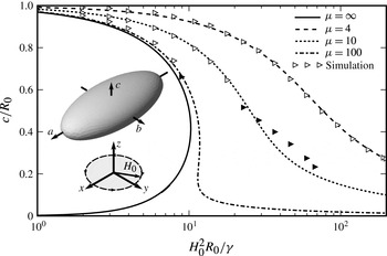
Figure 2 shows for several values of the magnetic permeability the analytic dependence of the ratio
 $c/R_{0}=K^{-2/3}$
on the magnetic Bond number
 $Bm=H_{0}^{2}R_{0}/\unicode[STIX]{x1D6FE}$
(
 $R_{0}^{3}=abc$
) (We have chosen to plot
 $c/R_{0}$
instead of
 $K$
since it remains a well defined quantity when the droplet takes a triaxial shape.). It shows that if the magnetic permeability is large enough, there is a hysteresis of
 $c/R_{0}$
as a function of the field. At infinite magnetic permeability an equilibrium shape, in the form of an oblate ellipsoid of revolution, only exists for magnetic fields below a critical field value.
In this respect the behaviour is similar to that of a conducting droplet in an electric field. An equilibrium shape, elongated along the field, only exists if the electric field strength is below a critical value (Taylor Reference Taylor1964). Above it there are jets appearing from the tips of the droplet.
Since in our case a fingering is observed experimentally (see figure 1 and Bacri et al. (Reference Bacri, Cebers and Perzynski1994)) on the perimeter of the disc-like droplet then it may be related to the threshold of existence of oblate equilibrium shape for large values of the magnetic permeability.
Normalized short axis of the oblate shape (
 $c/R_{0}$
) as a function of the magnetic Bond number for several values of
 $\unicode[STIX]{x1D707}=[4;10;100;\infty ]$
. Various lines are analytic calculations for ellipsoidal figures of equilibrium (obtained from § 2.3). Open triangles are the results of the numerical simulation of droplets with axial symmetry, while solid triangles mark the figures of equilibrium which take triaxial shape (see § 4).

By Bacri et al. (Reference Bacri, Cebers and Perzynski1994) (see Cebers & Lacis (Reference Cebers and Lacis1995) for more details) it was found during the analysis of the experimental results that the oblate shape loses its stability with respect to the symmetry-destroying perturbations, the long axis of the ellipsoid of revolution, remaining in the plane of the rotating field. The main conclusions included a critical value of the magnetic permeability for this instability and the re-entrant character of this oblate–prolate transition. This approach was further developed by Morozov & Lebedev (Reference Morozov and Lebedev2000) where a general ellipsoid with the semi-axes (
 $a>b>c$
) for symmetry-destroying perturbations was considered. The main features of the oblate–prolate transition, apart from the prediction of hysteresis in the oblate–prolate and the prolate–oblate transitions, qualitatively remained unchanged. Here we are using these results (see figure 3) for the comparison with the numerical simulation of the three-dimensional droplet and experiments (see ahead in figure 10). For completeness we give the main points of the analysis following the Morozov & Lebedev (Reference Morozov and Lebedev2000) approach. The energy of the droplet reads
 $$\begin{eqnarray}\displaystyle \frac{E}{2\unicode[STIX]{x03C0}\unicode[STIX]{x1D6FE}R_{0}^{2}} & = & \displaystyle \left(\frac{c^{2}}{ab}\right)^{2/3}\left(1+\frac{b}{\sqrt{a^{2}-c^{2}}}\left(\text{E}(k,m)\left(\frac{a^{2}}{c^{2}}-1\right)+\text{F}(k,m)\right)\right)\nonumber\\ \displaystyle & & \displaystyle -\,\frac{1}{6}Bm\unicode[STIX]{x1D712}\left(\frac{1}{1+4\unicode[STIX]{x03C0}\unicode[STIX]{x1D712}n_{x}}+\frac{1}{1+4\unicode[STIX]{x03C0}\unicode[STIX]{x1D712}n_{y}}\right),\end{eqnarray}$$
where
 $k=\arcsin \sqrt{1-c^{2}/a^{2}};m=(1-(c/b)^{2})/(1-(c/a)^{2})$
and
 $\text{E},\text{F}$
are the elliptic integrals. We are using relations (Beleggia, Graef & Millev Reference Beleggia, Graef and Millev2006) that express the demagnetizing field coefficients
 $n_{x},n_{y}$
in terms of the demagnetizing field coefficient
 $n_{z}$
:
 $$\begin{eqnarray}n_{z}(c/a,c/b)=\frac{1}{2}\int _{0}^{\infty }\frac{\text{d}u}{(u+1)^{3/2}((c^{2}u/a^{2}+1)(c^{2}u/b^{2}+1))^{1/2}};\end{eqnarray}$$
 $$\begin{eqnarray}n_{x}(c/a,c/b)=n_{z}(a/c,a/b);\quad n_{y}(c/a,c/b)=n_{z}(b/a,b/c).\end{eqnarray}$$
The equilibrium shapes are found by minimizing the energy of the droplet with respect to
 $c/a$
and
 $c/b$
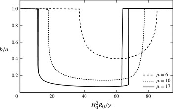
. The bifurcation diagram in coordinates
 $H_{0}^{2}R_{0}/\unicode[STIX]{x1D6FE}$
and
 $b/a$
for several
 $\unicode[STIX]{x1D707}$
values (
 $\unicode[STIX]{x1D707}=6,10,17$
) is given in figure 3. A hysteresis in the oblate–prolate–oblate transition at large values of the magnetic field strength emerges for large values of
 $\unicode[STIX]{x1D707}$
which is in accord with the results obtained by Morozov & Lebedev (Reference Morozov and Lebedev2000). For small field values the hysteresis is small. The calculations are in agreement with Morozov & Lebedev (Reference Morozov and Lebedev2000) and show that the transition from oblate to a triaxial ellipsoid exists above some critical value of the magnetic susceptibility (in the interval of
 $\unicode[STIX]{x1D707}$
 $[5;6]$
).
Axis ratio
 $b/a$
of a three-axis ellipsoid as a function magnetic Bond number for several values of magnetic permeability analytically calculated according to relation (2.22) with
 $\unicode[STIX]{x1D707}=17,10,6$
. This illustrates the transitions from oblate (
 $a=b$
) shape to triaxial ellipsoid and then back to oblate shape, according to Morozov & Lebedev (Reference Morozov and Lebedev2000). It shows a hysteresis at large magnetic Bond numbers for
 $\unicode[STIX]{x1D707}>11$
.

3 Numerical algorithm
3.1 Boundary-integral equations for magnetic field
Since
 $\unicode[STIX]{x1D735}\times \boldsymbol{H}=0$
, we recall that the magnetic field is potential
 $\boldsymbol{H}=\unicode[STIX]{x1D735}\unicode[STIX]{x1D713}$
and the potential due to
 $\unicode[STIX]{x1D735}\boldsymbol{\cdot }\boldsymbol{H}=0$
satisfies the Laplace equation
 $\unicode[STIX]{x0394}\unicode[STIX]{x1D713}=0$
. This equation can also be written in a boundary-integral form (Pozrikidis Reference Pozrikidis2003)
 $$\begin{eqnarray}\int _{\unicode[STIX]{x2202}\unicode[STIX]{x1D6FA}}\frac{\unicode[STIX]{x2202}\unicode[STIX]{x1D713}}{\unicode[STIX]{x2202}n_{\boldsymbol{x}}}\frac{1}{|\boldsymbol{x}-\boldsymbol{y}|}\,\text{d}S_{\boldsymbol{x}}-\int _{\unicode[STIX]{x2202}\unicode[STIX]{x1D6FA}}\unicode[STIX]{x1D713}(\boldsymbol{x})\frac{\unicode[STIX]{x2202}}{\unicode[STIX]{x2202}n_{\boldsymbol{x}}}\frac{1}{|\boldsymbol{x}-\boldsymbol{y}|}\,\text{d}S_{\boldsymbol{x}}=\left\{\begin{array}{@{}ll@{}}4\unicode[STIX]{x03C0}\unicode[STIX]{x1D713}(\boldsymbol{y}) & \text{if }\boldsymbol{y}\in \unicode[STIX]{x1D6FA}\\ 2\unicode[STIX]{x03C0}\unicode[STIX]{x1D713}(\boldsymbol{y}) & \text{if }\boldsymbol{y}\in \unicode[STIX]{x2202}\unicode[STIX]{x1D6FA}\\ 0 & \text{if }\boldsymbol{y}\ni \unicode[STIX]{x1D6FA},\end{array}\right.\end{eqnarray}$$
where
 $\unicode[STIX]{x1D6FA}$
is an arbitrary region where
 $\unicode[STIX]{x0394}\unicode[STIX]{x1D713}=0$
and
 $\unicode[STIX]{x2202}\unicode[STIX]{x1D6FA}$
denotes the boundary of the fluid drop. If
 $\boldsymbol{y}\in \unicode[STIX]{x2202}\unicode[STIX]{x1D6FA}$
the second integral from the left-hand side must be interpreted in the Cauchy principal value sense which we denote here as
 $\unicode[STIX]{x2A0D}$
.
Applying the boundary conditions
 $\unicode[STIX]{x1D713}^{(i)}=\unicode[STIX]{x1D713}^{(e)}$
and
 $\unicode[STIX]{x1D707}(\unicode[STIX]{x2202}\unicode[STIX]{x1D713}^{(i)}/\unicode[STIX]{x2202}n)=(\unicode[STIX]{x2202}\unicode[STIX]{x1D713}^{(e)}/\unicode[STIX]{x2202}n)$
for the boundary of fluid drop
 $\unicode[STIX]{x2202}\unicode[STIX]{x1D6FA}$
we obtain the following BIE for the magnetic potential (see appendix A)
 $$\begin{eqnarray}\unicode[STIX]{x1D713}(\boldsymbol{y})=\frac{2\boldsymbol{H}_{0}\boldsymbol{\cdot }\boldsymbol{y}}{\unicode[STIX]{x1D707}+1}-\frac{1}{2\unicode[STIX]{x03C0}}\frac{\unicode[STIX]{x1D707}-1}{\unicode[STIX]{x1D707}+1}\unicode[STIX]{x2A0D}_{\unicode[STIX]{x2202}\unicode[STIX]{x1D6FA}}\unicode[STIX]{x1D713}(\boldsymbol{x})\frac{\unicode[STIX]{x2202}}{\unicode[STIX]{x2202}n_{\boldsymbol{x}}}\frac{1}{|\boldsymbol{x}-\boldsymbol{y}|}\,\text{d}S_{\boldsymbol{x}},\end{eqnarray}$$
where
 $\boldsymbol{y}\in \unicode[STIX]{x2202}\unicode[STIX]{x1D6FA}$
. After solving this equation for
 $\unicode[STIX]{x1D713}$
we can use numerical differentiation to obtain the tangential components of the magnetic field
 $(\boldsymbol{I}-\boldsymbol{n}\otimes \boldsymbol{n})\boldsymbol{H}$
.
Numerous boundary-integral equations exist for the normal component of the magnetic field. One possibility is to use (3.1) for the normal component of the field with a known
 $\unicode[STIX]{x1D713}$
. However this gives an integral equation of the first kind and numerical experiments show a high sensitivity to the precision of the
 $\unicode[STIX]{x1D713}$
values. Another way is to formulate the boundary-integral equation for the normal field as previously done for fluid droplets suspended in an electric field by Baygents, Rivette & Stone (Reference Baygents, Rivette and Stone1998) (see also appendix A for derivation). However, it requires the integration of a strong singularity which is hard to do numerically in the general three-dimensional case. Eventually we settled on interpreting a perturbation of the magnetic field from the droplet as coming from the surface currents on its interface
 $4\unicode[STIX]{x03C0}\boldsymbol{K}/c=\boldsymbol{n}\times (\boldsymbol{B}^{(e)}-\boldsymbol{B}^{(i)})=-(\unicode[STIX]{x1D707}-1)\boldsymbol{n}\times \boldsymbol{H}$
.
The magnetic field outside the fluid droplet is given by the Biot–Savart integral
 $\boldsymbol{B}=\boldsymbol{B}_{0}+c^{-1}\int _{\unicode[STIX]{x2202}\unicode[STIX]{x1D6FA}}\boldsymbol{K}\times \unicode[STIX]{x1D735}_{\boldsymbol{x}}1/|\boldsymbol{x}-\boldsymbol{y}|\,\text{d}S_{\boldsymbol{x}}$
, which for the normal component of the magnetic field in the presence of an external field
 $\boldsymbol{H}_{0}$
gives
 $$\begin{eqnarray}\displaystyle \boldsymbol{B}\boldsymbol{\cdot }\boldsymbol{n}_{\boldsymbol{y}} & = & \displaystyle \boldsymbol{B}_{0}\boldsymbol{\cdot }\boldsymbol{n}_{\boldsymbol{y}}+\boldsymbol{n}_{\boldsymbol{y}}\boldsymbol{\cdot }\int _{\unicode[STIX]{x2202}\unicode[STIX]{x1D6FA}}\boldsymbol{K}\times \unicode[STIX]{x1D735}_{\boldsymbol{x}}\frac{1}{|\boldsymbol{x}-\boldsymbol{y}|}\,\text{d}S_{\boldsymbol{x}}=\boldsymbol{B}_{0}\boldsymbol{\cdot }\boldsymbol{n}_{\boldsymbol{y}}\nonumber\\ \displaystyle & & \displaystyle -\,\frac{\unicode[STIX]{x1D707}-1}{4\unicode[STIX]{x03C0}}\boldsymbol{n}_{\boldsymbol{y}}\boldsymbol{\cdot }\int _{\unicode[STIX]{x2202}\unicode[STIX]{x1D6FA}}(\boldsymbol{n}_{\boldsymbol{x}}\times \boldsymbol{H})\times \unicode[STIX]{x1D735}_{\boldsymbol{x}}\frac{1}{|\boldsymbol{x}-\boldsymbol{y}|}\,\text{d}S_{\boldsymbol{x}},\end{eqnarray}$$
which we also derive in appendix A without the use of the surface current interpretation. Since the integral on the right-hand side of relation (3.3) only has a cross-product of the field and the normal, it allows us to calculate the normal field component from the known tangential components. The numerical algorithm for this calculation is described in § 3.2.
3.2 Numerical implementation
Solving the BIE for the magnetic potential in the form (3.2) or integrating (3.3) would require singular integral quadrature which makes these equations hard to implement numerically. We overcome this difficulty using a singularity subtraction technique, which is a common practice in the application of the BIE (Keaveny & Shelley Reference Keaveny and Shelley2011). Specifically, for the magnetic potential we have an identity
 $\unicode[STIX]{x2A0D}(\unicode[STIX]{x2202}/\unicode[STIX]{x2202}n_{\boldsymbol{x}})(1/|\boldsymbol{x}-\boldsymbol{y}|)\,\text{d}S_{\boldsymbol{x}}=-2\unicode[STIX]{x03C0}$
(see appendix B) which we use to rewrite (3.2) in the following form
 $$\begin{eqnarray}\unicode[STIX]{x1D713}(\boldsymbol{y})\left(1-\frac{\unicode[STIX]{x1D707}-1}{\unicode[STIX]{x1D707}+1}\right)=\frac{2\boldsymbol{H}_{0}\boldsymbol{\cdot }\boldsymbol{y}}{\unicode[STIX]{x1D707}+1}-\frac{1}{2\unicode[STIX]{x03C0}}\frac{\unicode[STIX]{x1D707}-1}{\unicode[STIX]{x1D707}+1}\int _{\unicode[STIX]{x2202}\unicode[STIX]{x1D6FA}}\left[\unicode[STIX]{x1D713}(\boldsymbol{x})-\unicode[STIX]{x1D713}(\boldsymbol{y})\right]\frac{\unicode[STIX]{x2202}}{\unicode[STIX]{x2202}n_{\boldsymbol{x}}}\frac{1}{|\boldsymbol{x}-\boldsymbol{y}|}\,\text{d}S_{\boldsymbol{x}},\end{eqnarray}$$
where
 $\unicode[STIX]{x2A0D}\rightarrow \int$
since we reduced the singularity by one order. The discretization of the drop surface into plane triangles enables us to solve it for arbitrary geometries.
The simplest quadrature for triangles
 $\int _{\unicode[STIX]{x1D6E5}}f\,\text{d}S=(f_{1}+f_{2}+f_{3})S_{\unicode[STIX]{x1D6E5}}/3$
(trapezoidal quadrature) is used and it allows us to rearrange the integration efficiently. Denoting by
 $S_{j}$
the
 $1/3$
of the sum of the area of all triangles with a common vertex
 $j$
we can rewrite (3.4) in a discrete form
 $$\begin{eqnarray}\unicode[STIX]{x1D713}_{j}\left(1-\frac{\unicode[STIX]{x1D707}-1}{\unicode[STIX]{x1D707}+1}\right)=\frac{2\boldsymbol{H}_{0}\boldsymbol{\cdot }\boldsymbol{x}_{0}}{\unicode[STIX]{x1D707}+1}-\frac{1}{2\unicode[STIX]{x03C0}}\frac{\unicode[STIX]{x1D707}-1}{\unicode[STIX]{x1D707}+1}\mathop{\sum }_{i\neq j}[\unicode[STIX]{x1D713}_{i}-\unicode[STIX]{x1D713}_{j}]\frac{(\boldsymbol{x}_{j}-\boldsymbol{x}_{i})\boldsymbol{\cdot }\boldsymbol{n}_{j}}{|\boldsymbol{x}_{i}-\boldsymbol{x}_{j}|^{3}}S_{j},\end{eqnarray}$$
which we solve numerically with the LAPACK library. Using a triangulation of the ellipsoid (for which the normal vectors and the solution of the magnetostatic problem are known) we see that the solution is only moderately sensitive to the precision of the normal vectors. Therefore, we use a simple and robust method for calculating the vertex normal vectors (Jin, Lewis & West Reference Jin, Lewis and West2005) which is
 $$\begin{eqnarray}\boldsymbol{n}_{j}\propto \mathop{\sum }_{i}\unicode[STIX]{x1D6FC}_{i}\boldsymbol{n}_{i},\end{eqnarray}$$
where the summation is over the triangles which have a vertex
 $j$
. In relation (3.6)
 $\boldsymbol{n}_{i}$
is the normal to the plane triangle and
 $\unicode[STIX]{x1D6FC}_{i}$
is the angle of the triangle at the vertex
 $j$
.
In order to obtain the tangential components of the magnetic field we use the numerical differentiation of the obtained potential. For each vertex
 $j$
we write a system of equations
 $$\begin{eqnarray}(\unicode[STIX]{x1D735}\unicode[STIX]{x1D713})_{j}\boldsymbol{\cdot }(\boldsymbol{x}_{i}-\boldsymbol{x}_{j})=\unicode[STIX]{x1D713}_{i}-\unicode[STIX]{x1D713}_{j},\end{eqnarray}$$
where
 $i$
are the neighbour vertices. This system is overdetermined for the three components of
 $\unicode[STIX]{x1D735}\unicode[STIX]{x1D713}$
therefore the linear least squares method is applied. Tangential field components are then projected out of the estimated gradient
 $P\boldsymbol{H}_{j}=(\boldsymbol{I}-\boldsymbol{n}_{j}\otimes \boldsymbol{n}_{j})(\unicode[STIX]{x1D735}\unicode[STIX]{x1D713})_{j}$
, where
 $P=(\boldsymbol{I}-\boldsymbol{n}_{j}\otimes \boldsymbol{n}_{j})$
is the projection operator. The known tangential field components according to the relation (3.3) give us the normal component of the field as a Biot–Savart quadrature.
Since the quadrature in (3.3) is strongly singular it is inefficient to do it numerically in this form. The general procedure for subtracting the singularity in the Biot–Savart integral was given by Pozrikidis (Reference Pozrikidis2000), but it requires calculating the curvature by adding another issue of complexity. Instead of that we have developed a regularization technique which does not require a curvature calculation.
In the appendix B we prove the identity
 $$\begin{eqnarray}\displaystyle & & \displaystyle \unicode[STIX]{x2A0D}_{\unicode[STIX]{x2202}\unicode[STIX]{x1D6FA}}\unicode[STIX]{x1D735}_{\boldsymbol{x}}\frac{1}{|\boldsymbol{x}-\boldsymbol{y}|}\times (\boldsymbol{n}_{\boldsymbol{x}}\times \boldsymbol{H}_{\boldsymbol{x}})\,\text{d}S_{\boldsymbol{x}}=\unicode[STIX]{x2A0D}_{\unicode[STIX]{x2202}\unicode[STIX]{x1D6FA}}(P\boldsymbol{H}_{\boldsymbol{x}}-P\boldsymbol{H}_{\boldsymbol{y}})\times \left(\boldsymbol{n}_{\boldsymbol{x}}\times \unicode[STIX]{x1D735}_{\boldsymbol{x}}\frac{1}{|\boldsymbol{x}-\boldsymbol{y}|}\right)\text{d}S_{\boldsymbol{x}}\nonumber\\ \displaystyle & & \displaystyle \qquad -\,\unicode[STIX]{x2A0D}_{\unicode[STIX]{x2202}\unicode[STIX]{x1D6FA}}(P\boldsymbol{H}_{\boldsymbol{x}}-P\boldsymbol{H}_{\boldsymbol{y}})\left(\boldsymbol{n}_{\boldsymbol{x}}\boldsymbol{\cdot }\unicode[STIX]{x1D735}\frac{1}{|\boldsymbol{x}-\boldsymbol{y}|}\right)\text{d}S_{\boldsymbol{x}}-2\unicode[STIX]{x03C0}P\boldsymbol{H}_{\boldsymbol{y}},\end{eqnarray}$$
where
 $PH_{\boldsymbol{y}}$
is a constant vector. This identity enables us to evaluate the strongly singular quadrature on the left-hand side of relation (3.8) with weakly singular quadratures on its right-hand side. Using this formula for (3.3) gives us weakly singular form of Biot–Savart quadrature
 $$\begin{eqnarray}\displaystyle & & \displaystyle \boldsymbol{B}\boldsymbol{\cdot }\boldsymbol{n}_{\boldsymbol{y}}=\boldsymbol{H}_{0}\boldsymbol{\cdot }\boldsymbol{n}_{\boldsymbol{y}}-\frac{\unicode[STIX]{x1D707}-1}{4\unicode[STIX]{x03C0}}\boldsymbol{n}_{\boldsymbol{y}}\boldsymbol{\cdot }\unicode[STIX]{x2A0D}_{\unicode[STIX]{x2202}\unicode[STIX]{x1D6FA}}(P\boldsymbol{H}_{\boldsymbol{x}}-P\boldsymbol{H}_{\boldsymbol{y}})\times \left(\boldsymbol{n}_{\boldsymbol{x}}\times \unicode[STIX]{x1D735}_{\boldsymbol{x}}\frac{1}{|\boldsymbol{x}-\boldsymbol{y}|}\right)\text{d}S_{\boldsymbol{x}}\nonumber\\ \displaystyle & & \displaystyle \qquad +\,\frac{\unicode[STIX]{x1D707}-1}{4\unicode[STIX]{x03C0}}\boldsymbol{n}_{\boldsymbol{y}}\boldsymbol{\cdot }\unicode[STIX]{x2A0D}_{\unicode[STIX]{x2202}\unicode[STIX]{x1D6FA}}(P\boldsymbol{H}_{\boldsymbol{x}}-P\boldsymbol{H}_{\boldsymbol{y}})\left(\boldsymbol{n}_{\boldsymbol{x}}\boldsymbol{\cdot }\unicode[STIX]{x1D735}\frac{1}{|\boldsymbol{x}-\boldsymbol{y}|}\right)\text{d}S_{\boldsymbol{x}}.\end{eqnarray}$$
We integrate both integrals of (3.9) with the trapezoidal rule for non-singular integrals and use a polar transformation for weakly singular integrals (Pozrikidis Reference Pozrikidis2003). Specifically, when the singularity is on
 $\boldsymbol{x}_{1}$
we have the quadrature formula
 $$\begin{eqnarray}\left.\begin{array}{@{}c@{}}\displaystyle \int _{\unicode[STIX]{x1D6E5}}{\displaystyle \frac{q(\boldsymbol{x})}{|\boldsymbol{x}-\boldsymbol{x}_{1}|}}\,\text{d}S_{\boldsymbol{x}}={\displaystyle \frac{|(\boldsymbol{x}_{2}-\boldsymbol{x}_{1})\times (\boldsymbol{x}_{3}-\boldsymbol{x}_{1})|}{|\boldsymbol{x}_{2}-\boldsymbol{x}_{1}|}}\int _{0}^{\unicode[STIX]{x03C0}/2}{\displaystyle \frac{\int _{0}^{1/(\cos \unicode[STIX]{x1D712}+\sin \unicode[STIX]{x1D712})}q(\unicode[STIX]{x1D70C},\unicode[STIX]{x1D712})\,\text{d}\unicode[STIX]{x1D70C}}{\sqrt{\cos ^{2}\unicode[STIX]{x1D712}+B\sin 2\unicode[STIX]{x1D712}+C\sin ^{2}\unicode[STIX]{x1D712}}}}\,\text{d}\unicode[STIX]{x1D712}\\ \boldsymbol{x}=\unicode[STIX]{x1D70C}\cos \unicode[STIX]{x1D712}\boldsymbol{x}_{1}+\unicode[STIX]{x1D70C}\sin \unicode[STIX]{x1D712}\boldsymbol{x}_{2}+(1-\unicode[STIX]{x1D70C}(\cos \unicode[STIX]{x1D712}+\sin \unicode[STIX]{x1D712}))\boldsymbol{x}_{3}\\ q=\unicode[STIX]{x1D70C}\cos \unicode[STIX]{x1D712}q_{1}+\unicode[STIX]{x1D70C}\sin \unicode[STIX]{x1D712}q_{2}+(1-\unicode[STIX]{x1D70C}(\cos \unicode[STIX]{x1D712}+\sin \unicode[STIX]{x1D712}))q_{3}\\ B=(\boldsymbol{x}_{2}-\boldsymbol{x}_{1})\boldsymbol{\cdot }(\boldsymbol{x}_{2}-\boldsymbol{x}_{1})/|\boldsymbol{x}_{2}-\boldsymbol{x}_{1}|^{2};\quad C=|\boldsymbol{x}_{3}-\boldsymbol{x}_{1}|^{2}/|\boldsymbol{x}_{2}-\boldsymbol{x}_{1}|^{2},\end{array}\right\}\end{eqnarray}$$
where we use a Gauss–Legendre quadrature with
 $10$
points for the
 $\unicode[STIX]{x1D70C}$
and
 $\unicode[STIX]{x1D712}$
variables.
Besides the magnetic field another important quantity for the surface force calculation is the curvature as can be seen in (2.17). However, it turns out that the explicit mean curvature calculation can be avoided since we are interested in an integral containing a curvature over a closed surface. In Pozrikidis (Reference Pozrikidis2001), Zinchenko, Rother & Davis (Reference Zinchenko, Rother and Davis1997) and appendix C the following identity is derived for the value of the integral at a surface point with the radius vector
 $\boldsymbol{y}$
(
 $\boldsymbol{r}=\boldsymbol{x}-\boldsymbol{y}$
)
 $$\begin{eqnarray}\displaystyle \int \left({\displaystyle \frac{1}{R_{1}}}+{\displaystyle \frac{1}{R_{2}}}\right)\boldsymbol{n}_{\boldsymbol{y}} & \boldsymbol{\cdot } & \displaystyle \left(\frac{\boldsymbol{I}}{r}+\frac{\boldsymbol{r}\otimes \boldsymbol{r}}{r^{3}}\right)\boldsymbol{\cdot }\boldsymbol{n}_{\boldsymbol{x}}\,\text{d}S_{\boldsymbol{x}}=-\int \frac{\boldsymbol{r}\boldsymbol{\cdot }(\boldsymbol{n}_{\boldsymbol{x}}+\boldsymbol{n}_{\boldsymbol{y}})}{r^{3}}\nonumber\\ \displaystyle & \boldsymbol{\cdot } & \displaystyle \left(1-\frac{3(\boldsymbol{r}\boldsymbol{\cdot }\boldsymbol{n}_{\boldsymbol{x}})(\boldsymbol{r}\boldsymbol{\cdot }\boldsymbol{n}_{\boldsymbol{y}})}{r^{2}}\right)\text{d}S_{\boldsymbol{x}}.\end{eqnarray}$$
Putting this formula in (2.17), (2.18) and using the identity
 $\int (\boldsymbol{I}/r+\boldsymbol{r}\otimes \boldsymbol{r}/r^{3})\boldsymbol{\cdot }\boldsymbol{n}_{\boldsymbol{x}}\,\text{d}S_{\boldsymbol{x}}=0$
for the singularity subtraction we get the normal component of the velocity
 $$\begin{eqnarray}\bar{f}=\frac{1-1/\unicode[STIX]{x1D707}}{8\unicode[STIX]{x03C0}}B_{n}^{2}+\frac{\unicode[STIX]{x1D707}-1}{8\unicode[STIX]{x03C0}}H_{t}^{2};\end{eqnarray}$$
 $$\begin{eqnarray}\displaystyle \boldsymbol{v}\boldsymbol{\cdot }\boldsymbol{n}_{\boldsymbol{y}} & = & \displaystyle \frac{1}{8\unicode[STIX]{x03C0}\unicode[STIX]{x1D702}}\int _{\unicode[STIX]{x2202}\unicode[STIX]{x1D6FA}}\left(\frac{\boldsymbol{n}_{\boldsymbol{x}}\boldsymbol{\cdot }\boldsymbol{n}_{\boldsymbol{y}}}{r}+\frac{(\boldsymbol{r}\boldsymbol{\cdot }\boldsymbol{n}_{\boldsymbol{x}})(\boldsymbol{r}\boldsymbol{\cdot }\boldsymbol{n}_{\boldsymbol{y}})}{r^{3}}\right)(\,\,\bar{f}_{\boldsymbol{x}}-\bar{f}_{\boldsymbol{y}})\,\text{d}S_{\boldsymbol{x}}\nonumber\\ \displaystyle & & \displaystyle +\,\frac{\unicode[STIX]{x1D6FE}}{8\unicode[STIX]{x03C0}\unicode[STIX]{x1D702}}\int _{\unicode[STIX]{x2202}\unicode[STIX]{x1D6FA}}\frac{\boldsymbol{r}\boldsymbol{\cdot }(\boldsymbol{n}_{\boldsymbol{x}}+\boldsymbol{n}_{\boldsymbol{y}})}{r^{3}}\left(1-\frac{3(\boldsymbol{r}\boldsymbol{\cdot }\boldsymbol{n}_{\boldsymbol{x}})(\boldsymbol{r}\boldsymbol{\cdot }\boldsymbol{n}_{\boldsymbol{y}})}{r^{2}}\right)\text{d}S_{\boldsymbol{x}}.\end{eqnarray}$$
Using the trapezoidal integration formula for all triangular elements for both integrals we obtain the normal component of the velocity which we use to proceed to the next time step.
3.3 Averaged equations for high frequency
As noted in § 1 we are interested in the behaviour of the droplets in a rotating field with a high frequency. In this limit we can neglect the droplet shape variation during the field period. At equal droplet and surrounding fluid viscosities the numerical simulations have shown that the high-frequency behaviour establishes at
 $\unicode[STIX]{x1D714}\gg 10R_{0}\unicode[STIX]{x1D702}/\unicode[STIX]{x1D6FE}$
.
To derive the corresponding high-frequency equations let us set, as previously, the magnetic field rotation plane as the (
 $x,y$
) plane
 $$\begin{eqnarray}\boldsymbol{H}_{0}=H_{0}\cos (\unicode[STIX]{x1D714}t)\boldsymbol{e}_{x}+H_{0}\sin (\unicode[STIX]{x1D714}t)\boldsymbol{e}_{y}.\end{eqnarray}$$
Because of the superposition principle we can write a solution of the magnetostatic equations
 $$\begin{eqnarray}\boldsymbol{H}(\boldsymbol{x},\boldsymbol{H}_{0})=H_{0}\cos (\unicode[STIX]{x1D714}t)\boldsymbol{H}_{x}+H_{0}\sin (\unicode[STIX]{x1D714}t)\boldsymbol{H}_{y},\end{eqnarray}$$
where we set
 $\boldsymbol{H}_{x}=\boldsymbol{H}(\boldsymbol{x},\boldsymbol{e}_{x})$
and
 $\boldsymbol{H}_{y}=\boldsymbol{H}(\boldsymbol{x},\boldsymbol{e}_{y})$
. With this solution we can now write the normal component of the instantaneous magnetic surface force (3.12) as
 $$\begin{eqnarray}\bar{f}=\frac{1-1/\unicode[STIX]{x1D707}}{8\unicode[STIX]{x03C0}}(H_{0}\cos (\unicode[STIX]{x1D714}t)B_{xn}+H_{0}\sin (\unicode[STIX]{x1D714}t)B_{yn})^{2}+\frac{\unicode[STIX]{x1D707}-1}{8\unicode[STIX]{x03C0}}(H_{0}\cos (\unicode[STIX]{x1D714}t)P\boldsymbol{H}_{x}+H_{0}\sin (\unicode[STIX]{x1D714}t)P\boldsymbol{H}_{y})^{2}.\end{eqnarray}$$
Averaging this force over a single period gives us
 $$\begin{eqnarray}\langle \,\bar{f}\rangle =\frac{1-1/\unicode[STIX]{x1D707}}{16\unicode[STIX]{x03C0}}H_{0}^{2}(B_{xn}^{2}+B_{yn}^{2})+\frac{\unicode[STIX]{x1D707}-1}{16\unicode[STIX]{x03C0}}H_{0}^{2}(H_{xt}^{2}+H_{yt}^{2}),\end{eqnarray}$$
which can be inserted in (3.13) to obtain the average normal velocity in high-frequency rotating field.
3.4 Mesh maintenance and generation
Within a small number of time steps, at which the surface markers were advanced, an uneven triangulation is produced. It makes the representation of the geometry unsatisfactory due to degenerate triangular elements affecting the precision of the force and velocity calculation. To overcome this difficulty mesh relaxation and stabilization methods have been used for viscous drop simulations in Cristini, Bławzdziewicz & Loewenberg (Reference Cristini, Bławzdziewicz and Loewenberg2001) and Zinchenko, Rother & Davis (Reference Zinchenko, Rother and Davis1999). Here we use a general purpose mesh stabilization/relaxation algorithm by Brochu & Bridson (Reference Brochu and Bridson2009), which is also available as an open source library named ElTopo.
This algorithm collapses edges which are smaller than
 $l_{min}$
, splits those which are larger than
 $l_{max}$
and flips edges if after an operation they become shorter. The algorithm also moves each vertex to its average of neighbour vertices while the movement of vertex is restricted to its estimated normal plane.
To ensure that these operations do preserve sharp features in places with a high curvature they are allowed only if the volume changes introduced by any operation are smaller than
 $\unicode[STIX]{x1D6FE}_{vol}$
. Also, to avoid generation of new degenerate triangles, an operation is not allowed if it introduces triangles with an angle either smaller than
 $\unicode[STIX]{x1D6FC}_{min}$
or larger than
 $\unicode[STIX]{x1D6FC}_{max}$
. In our studies we used the following set of mesh configuration maintenance parameters
 $$\begin{eqnarray}l_{min}=0.7\unicode[STIX]{x1D709};\quad l_{max}=1.5\unicode[STIX]{x1D709};\quad \unicode[STIX]{x1D6FE}_{vol}=0.1\unicode[STIX]{x1D709}^{3};\quad \unicode[STIX]{x1D6FC}_{min}=15^{0};\quad \unicode[STIX]{x1D6FC}_{max}=120^{0},\end{eqnarray}$$
where we set
 $\unicode[STIX]{x1D709}$
as the average edge length of the initial mesh.
We used a simple Euler method for advancing markers to new positions and used a sufficiently small time step so that the volume changes are less than 1 % when the equilibrium is obtained. We observed that large time steps could also induce a random noise and that the main limitation for the step size comes from the higher chance of getting a degenerate mesh in the middle of a simulation.
For starting the simulation we need an initial triangulation. We used the Distmesh library developed by Persson & Strang (Reference Persson and Strang2004) for generating the initial triangulation from the analytical signed distance functions taking only the average edge length
 $\unicode[STIX]{x1D709}$
as an argument. With this algorithm we successfully generated high quality meshes for spheres, ellipsoids and star-like shapes.
4 Numerical simulation results
4.1 Worm-like equilibrium figures
The compression of the droplet perpendicularly to the plane of the rotating field was used as a test for the developed algorithm along with smaller tests for droplet extension in a constant field, relaxation dynamics and magnetic field calculation for the ellipsoid.
The procedure for finding the figures of equilibrium is as follows. Starting with initial triangulation we let the simulation algorithm relax the shape until the following conditions are met
 $$\begin{eqnarray}\frac{v_{i}}{v_{start}}<0.01;\quad \unicode[STIX]{x1D70F}_{i}v_{i}<0.01R_{0};\quad \unicode[STIX]{x1D70F}_{i}=\frac{\unicode[STIX]{x0394}t}{\log {\displaystyle \frac{v_{i-1}}{v_{i}}}},\end{eqnarray}$$
where
 $\unicode[STIX]{x0394}t$
is the time step,
 $v_{i}$
is the maximum velocity at the step
 $i$
and
 $v_{start}$
is the velocity when the relaxation of triangulation begins. First condition ensures that the velocities start to decay exponentially which is expected when the surface is close to an equilibrium. The second condition, assuming that equilibrium is approached exponentially, requires that the maximum deviation from true equilibrium (when
 $t\rightarrow \infty$
), for any point on the surface, is smaller than
 $1/100$
of
 $R_{0}$
.
For obtaining figures of equilibrium we used two methods. In the simplest one (ellipsoid relaxation) we started from an ellipsoid with semi-axes calculated by the energy (2.22) minimization. In the second more complex one (quasi-static simulation) we start from triangulation of a sphere and increase the magnetic field quasi-statically (
 $\unicode[STIX]{x0394}Bm=1$
) letting the triangulation relax at each step until condition (4.1) is met.
We induced a spontaneous symmetry breaking of an axial figure, in a quasi-static simulation, by stretching the triangulation in the
 $x$
axis direction and compressing it in the
 $y$
and
 $z$
axis directions to conserve the volume at the beginning of each quasi-step. When the difference between the lengths in the
 $x$
and
 $y$
directions became larger than
 $0.01R_{0}$
we disabled this part of the algorithm. By disabling we kept triangulation more regular which, as we observed, slightly affects simulated equilibrium figures. We observed that more time steps are necessary for a quasi-step when the transition to a triaxial figure is approached. The figures of equilibrium obtained with this algorithm at
 $\unicode[STIX]{x1D707}=10$
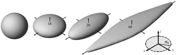
for different magnetic Bond numbers are shown in figure 4.
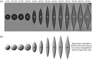
Sequence of the established figures of equilibrium found numerically at different magnetic Bond numbers (0, 18, 20, 68) with
 $\unicode[STIX]{x1D707}=10$
.

However, some differences are observed depending on how the axial symmetry-destroying perturbations are imposed – ellipsoid relaxation or quasi-static simulation. Equilibrium shapes calculated by ellipsoid relaxation method are in excellent agreement with analytical results and also with experiments (as we will see in § 5). The numerical experiments show that the difference between the figures of equilibrium obtained by ellipsoidal relaxation and by quasi-static simulation is due to an overly coarse triangulation and the quality of the mesh.
4.2 Star-like equilibrium figures
Even if we do not manage to induce the star-like instability with numerical simulations directly from a worm-like figure, we are able to make a simulation of a star-like equilibrium figure, if we initially start with a mesh which has a broken symmetry at the starting point. As a seed we use the following surface
 $$\begin{eqnarray}x^{2}+y^{2}+4z^{2}-\cos ^{2}\left(3\arctan \frac{y}{x}\right)\frac{x^{2}+y^{2}}{x^{2}+y^{2}+z^{2}}=1,\end{eqnarray}$$
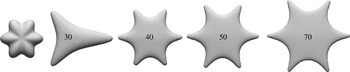
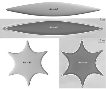
which we meshed with the Distmesh library (Persson & Strang Reference Persson and Strang2004). We instantly set a magnetic field and depending on its strength we obtain the star-like equilibrium figures (see figure 5).
Initial six-pointed star seed for simulations (left) and star-like droplet shapes obtained numerically at different magnetic Bond numbers with
 $\unicode[STIX]{x1D707}=10$
.

For small magnetic Bond numbers
 $Bm<19$
the perturbation decays and we obtain an axisymmetric oblate shape. At
 $Bm=30$
the six-pointed star perturbation still decays, but due to some imperfections in the initial mesh we obtain a triangular shape. Starting from magnetic Bond number
 $40$
we see that the six-pointed star perturbation grows for larger magnetic Bond numbers. Qualitatively the simulated star-like figures for different magnetic Bond numbers differ by their sizes in the
 $(x,y)$
plane but keep the length of the peaks approximately constant.
With higher magnetic Bond numbers up to
 $100$
we were not able to show that the initial higher-order perturbation decays. Instead some higher-order perturbations determine the shape of the droplet as we expected from the experiment. However, we did calculate energies for the stars. Within error bars they agree with the quasi-static simulations for
 $Bm\leqslant 50$
. However at
 $Bm=70$
we get an energy
 $E/4\unicode[STIX]{x03C0}R_{0}^{2}\unicode[STIX]{x1D6FE}=-3.15$
for the star, where for the worm-like shape we obtain
 $E/4\unicode[STIX]{x03C0}R_{0}^{2}\unicode[STIX]{x1D6FE}=-2.98$
. (For numerical energy calculation we used formula (4.4). We tested this formula with ellipsoidal meshes. Comparing with analytical formula (2.19) the error for the magnetic part was found to be approximately 2 % for a mesh with
 $3000$
triangles.) Thus, the star-like shape has a smaller energy than the worm-like shape for magnetic Bond numbers
 $Bm\geqslant 70$
. We can also conclude that by increasing the magnetic Bond number, the number of stable shapes increases while in the experiment we observe only two, when a hysteresis at the re-entrant transition happens.
4.3 Numerical tests and results
For the ratio
 $c/R_{0}$
, which characterizes the compression of the droplet in a rotating field and is calculated according to relation (2.21), we see a qualitatively good agreement between the numerical results and the analytic ellipsoidal approximation in a wide range of
 $\unicode[STIX]{x1D707}$
values as shown in figure 2. Specifically when
 $\unicode[STIX]{x1D707}=4$
the axially symmetric state of the droplet remains stable – the result which was predicted analytically for the droplet with an oblate ellipsoidal shape.
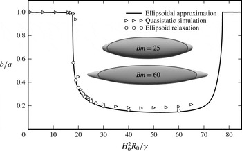
Axis ratio of the droplet in the plane of the rotating field as a function of the magnetic Bond number with
 $\unicode[STIX]{x1D707}=10$
. Full line: analytical calculation using ellipsoidal approximation (see § 2.3). Open circles – numerical data obtained by ellipsoidal relaxation, triangles – numerical data obtained by quasi-static simulation. Equilibrium figures obtained by numerical simulation with ellipsoid relaxation are shown in the figure. On top of them we have drawn ellipses to better see deviations at the tips.

On the other hand while the droplet keeps an ellipsoidal shape we may use the formula (2.22) for calculating the axis ratio in the plane of rotating field as can be seen in figure 6. We observe that the axis ratio
 $b/a$
starts to deviate from
 $1$
exactly where the ellipsoidal approximation predicts a transition from an oblate ellipsoid to a triaxial one. We also see that both simulations very well agree with the analytic ellipsoidal approximation as expected since droplet in simulation keeps a quasi-ellipsoidal shape. For large magnetic Bond numbers the quasi-static simulation becomes unreliable because of mesh quality loss and in figure 6 we can see its growing difference with ellipsoid relaxation simulation.
Figure 6 also presents two calculated (ellipsoid relaxation) equilibrium figures with ellipses drawn on the top of them to show better their deviations. We can see that figures of equilibrium starts to deviate significantly from the ellipsoidal shape for large magnetic fields, forming sharp tips as it is also observed in the experiments (figure 1). Unexpectedly, the simulation closely follows the analytic ellipsoidal approximation even for large magnetic fields where the droplet presents tips. Thus we can use the ellipsoidal approximation quantitatively for adjusting the experimental data.
We also calculate energies of the equilibrium figures and compare them with the energies found analytically in the ellipsoidal approximation (2.22). This latter should be larger or equal due to constraints. The total instantaneous energy of the drop is the sum of the surface energy
 $E_{S}=\unicode[STIX]{x1D6FE}S$
and the magnetization energy
 $E_{M}$
(2.13)
 $$\begin{eqnarray}E=\unicode[STIX]{x1D6FE}S-\frac{1}{2}\int _{\unicode[STIX]{x1D6FA}}\boldsymbol{M}\boldsymbol{\cdot }\boldsymbol{H}_{0}\text{d}V=\unicode[STIX]{x1D6FE}S-\frac{\unicode[STIX]{x1D707}-1}{8\unicode[STIX]{x03C0}}\int _{\unicode[STIX]{x1D6FA}}\boldsymbol{H}\boldsymbol{\cdot }\boldsymbol{H}_{0}\text{d}V=\unicode[STIX]{x1D6FE}S-\frac{\unicode[STIX]{x1D707}-1}{8\unicode[STIX]{x03C0}}\int _{\unicode[STIX]{x2202}\unicode[STIX]{x1D6FA}}\unicode[STIX]{x1D713}\boldsymbol{H}_{0}\boldsymbol{\cdot }\boldsymbol{n}_{\boldsymbol{x}}\,\text{d}S_{\boldsymbol{x}}.\end{eqnarray}$$
Since we consider the high-frequency limit of a rotating field, then according to the superposition principle (3.15), we write the average energy per period in the following way
 $$\begin{eqnarray}\langle E\rangle =\unicode[STIX]{x1D6FE}\int _{\unicode[STIX]{x2202}\unicode[STIX]{x1D6FA}}\,\text{d}S_{\boldsymbol{x}}-\frac{\unicode[STIX]{x1D707}-1}{8\unicode[STIX]{x03C0}}\frac{H_{0}^{2}}{2}\int _{\unicode[STIX]{x2202}\unicode[STIX]{x1D6FA}}(\unicode[STIX]{x1D713}_{x}\boldsymbol{e}_{x}+\unicode[STIX]{x1D713}_{y}\boldsymbol{e}_{y})\boldsymbol{\cdot }\boldsymbol{n}_{\boldsymbol{x}}\,\text{d}S_{\boldsymbol{x}},\end{eqnarray}$$
where
 $\unicode[STIX]{x1D713}_{x}(\boldsymbol{x})=\unicode[STIX]{x1D713}(\boldsymbol{e}_{x},\boldsymbol{x})$
is the potential for a unit field directed along the
 $x$
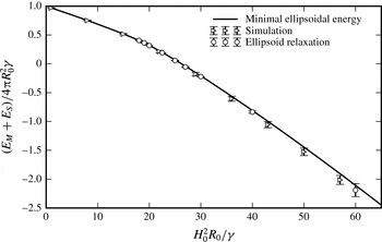
axis. Numerical integration with the trapezoidal rule (4.4) for each time step showed that the energy decreases monotonously until it reaches its equilibrium value. We plot equilibrium energies in figure 7 where we see that the energies of equilibrium shapes obtained in the quasi-static simulation and in the ellipsoidal approximation (2.22) are within the error bars equal to the analytically calculated energy. The main contribution to the error comes from its magnetic part. For mesh with 3000 triangles it equals 2 %.
Energy of droplets as a function of the magnetic Bond number. Comparison between numerical simulations with two different scenarios of inducing the symmetry-destroying perturbations and analytical calculation for droplets of ellipsoidal shapes with
 $\unicode[STIX]{x1D707}=10$
. Triangles are the results of numerical simulation by inducing symmetry-destroying perturbations as described in § 4 and circles starting from triangulation of three axis ellipsoids with semi-axes are calculated by the energy minimization. Solid line is deduced from the minimization of the energy given by (2.22). Difference is due to the non-uniformity of mesh in the first case.

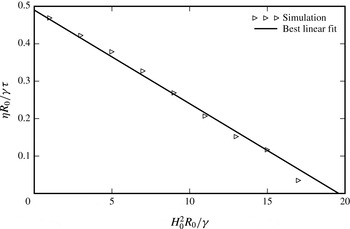
As a last numerical result, we show here that the critical slowing down is a useful tool for the calculation of the critical magnetic field associated with the threshold of triaxial ellipsoidal shape. By analogy with (Cebers & Zemitis Reference Cebers and Zemitis1983) we can estimate the critical Bond number by calculating the decrement of the symmetry-breaking perturbations going to zero due to the critical slowing down at the bifurcation value of the magnetic Bond number. Using a simulation with
 $\unicode[STIX]{x1D707}=10$
, which is close to the value for droplets used in experiments, we estimate the inverse of the logarithmic decrement
 $\unicode[STIX]{x1D70F}$
just before we jump to the next quasi-step. This decrement is drawn in figure 8 in a normalized form. We clearly see that the drop shape with an axial symmetry becomes unstable at approximately
 $Bm=19{-}20$
agreeing with result from the ellipsoidal approximation and simulation (figure 6).
Critical slowing down of relaxation of axial symmetry destroying perturbations in dependence on the magnetic Bond number.
 $\unicode[STIX]{x1D707}=10$
. Triangles are the results of numerical simulation.

5 Experiments and their comparison with numerical simulation
5.1 Preparation of magnetic droplets
Magnetic droplets can be prepared in various ways. The most common method is to disperse a magnetic fluid in an immiscible liquid (Zakinyan & Dikansky Reference Zakinyan and Dikansky2011). Recently an interesting system was used where drops in glycerine were formed by magnetic nanoparticles with a biocompatible polydimethylsiloxane (PDMS) coating without a carrying liquid (Afkami et al.
Reference Afkami, Tyler, Renardy, Renardy, Pierre, Woodward and Riffle2010). However, here we use magnetic drops that are obtained by inducing a phase separation in a magnetic fluid via an increase of ionic strength. The water-based magnetic fluid is prepared in the PHENIX laboratory, using the precipitation method (Massart Reference Massart1981), and has maghemite nanoparticles with a size
 $d=7.1$
nm and polydispersity
 $\unicode[STIX]{x1D70E}_{PDI}=0.32$
, volume fraction
 $\unicode[STIX]{x1D6F7}=2.8$
%, volume susceptibility
 $\unicode[STIX]{x1D712}=0.016$
(CGS units) and saturation magnetization
 $M_{sat}=8.4$
G at
 $H_{sat}=10$
kOe, as given by magnetization measurements. The colloidal particles are stabilized with citrate ions from trisodium citrate, which is added in excess, creating a large initial ionic strength
 $I_{citr}=0.18$
M present in the magnetic fluid. By adding 0.05 M of sodium chloride a phase separation is induced and droplets of concentrated phase are formed in the dilute phase. As the droplets have a larger concentration of magnetic nanoparticles than the surrounding liquid in coexistence and a low surface tension, droplets respond to an external magnetic field of low amplitude. A volume of
 ${\approx}25~\unicode[STIX]{x03BC}\text{l}$
of the phase separated fluid is put in quartz cuvettes of
 $0.1$
mm thickness (Hellma Analytics). The sample is then investigated using the experimental set-up.
5.2 Experimental set-up
The experimental set-up is based on a ZEISS Axio Observer.D1 microscope equipped with a custom-built coil system. Coils are powered by two KEPCO BOP 20-10ML power supplies and controlled by an NI DAQ system. The system has been calibrated with a gaussmeter, to link the magnetic field with current measurements. Images are recorded with AVT Guppy F-046B (8-bit greyscale, resolution
 $640\times 480$
px, frame rate 3.75 Hz). All devices are governed by a custom-built program in NI LabVIEW. The system enables us to apply constant and alternating fields in the image plane. A more detailed description of the experimental system and methods can be found in Kitenbergs (Reference Kitenbergs2015).
Recorded images are processed with MATLAB®. They are first thresholded to binary images for detecting individual objects. Then, to remove noise, dirt and other small drops, the largest object is selected and its perimeter is traced. Ellipse semi-axes
 $a$
and
 $b$
are found in the following way: the longest distance between two points of the perimeter is
 $2a$
, while
 $2b$
is measured perpendicularly to the midpoint of
 $2a$
.
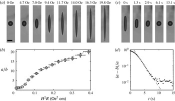
An elongation–relaxation experiment with a typical droplet of initial diameter
 $R=10~\unicode[STIX]{x03BC}\text{m}$
and its analysis to obtain the properties of the drop (see text for details). (a,c) Pictures of the evolution (a) of the drop elongation under stepwise field increasing and of the temporal relaxation (c) of the droplet in zero field – scale bar is
 $20~\unicode[STIX]{x03BC}\text{m}$
. (b,d) Evolution (b) of the droplet aspect ratio
 $a/b$
as a function of reduced field
 $H^{2}R$
and time relaxation (d) of the ratio
 $(a-b)/a$
in zero field. Dashed lines are adjustments by (5.1), (5.2) and (5.3).

5.3 Properties of magnetic droplets in constant field
One way to experimentally obtain the physical properties of a magnetic drop, namely surface tension
 $\unicode[STIX]{x1D6FE}$
, magnetic permeability
 $\unicode[STIX]{x1D707}$
and viscosity
 $\unicode[STIX]{x1D702}$
, is to make an elongation–relaxation experiment with subsequent analysis, as shown in figure 9. For the elongation part, the magnetic drop is gradually deformed under a stepwise increase of a homogeneous and static magnetic field, with its direction in the image plane (figure 9(a), parallel to the long side of the image). After each step an image and current measurements are recorded once the steady state has been reached. Image and data processing allows to form a plot of the ratio
 $a/b$
as a function of magnetic field, as shown in figure 9(b). The data are then adjusted with the equation from Bacri & Salin (Reference Bacri and Salin1982) and Cebers (Reference Cebers1985), assuming an ellipsoidal shape of revolution and a constant volume for the droplet:
 $$\begin{eqnarray}\displaystyle H^{2}R=\unicode[STIX]{x1D6FE}\left[{\displaystyle \frac{4\unicode[STIX]{x03C0}}{\unicode[STIX]{x1D707}-1}}+N\right]^{2}{\displaystyle \frac{1}{2\unicode[STIX]{x03C0}}}{\displaystyle \frac{\left({\displaystyle \frac{3-2e^{2}}{e^{2}}}-{\displaystyle \frac{(3-4e^{2})\arcsin e}{e^{3}(1-e^{2})^{1/2}}}\right)}{(1-e^{2})^{2/3}\left({\displaystyle \frac{(3-e^{2})}{e^{5}}}\ln \left({\displaystyle \frac{1+e}{1-e}}\right)-{\displaystyle \frac{6}{e^{4}}}\right)}},\end{eqnarray}$$
where
 $e$
is the ellipse eccentricity
 $(e=\sqrt{1-b^{2}/a^{2}})$
and
 $N$
its demagnetizing coefficient, which can be expressed for a prolate ellipsoid of revolution in the following way
 $$\begin{eqnarray}N=\frac{4\unicode[STIX]{x03C0}(1-e^{2})}{2e^{3}}\left(\ln \frac{1+e}{1-e}-2e\right).\end{eqnarray}$$
Equation (5.1) allows us to obtain the
 $\unicode[STIX]{x1D6FE}$
and
 $\unicode[STIX]{x1D707}$
values.
For the relaxation part, the magnetic field is cut to zero after a sufficient elongation and the droplet is allowed to relax back to a spherical shape. Its relaxation is recorded over time (figure 9
c). Close to a spherical shape, the parameter
 $(a-b)/a$
follows an exponential decay with a characteristic time
 $\unicode[STIX]{x1D70F}_{\unicode[STIX]{x1D702}}$
as illustrated by figure 9(d). In these experiments
 $(a-b)/a<0.02$
is the resolution limit,
 $\unicode[STIX]{x1D70F}_{\unicode[STIX]{x1D702}}$
is described with an equation from Dikansky, Cebers & Shatsky (Reference Dikansky, Cebers and Shatsky1990):
 $$\begin{eqnarray}\unicode[STIX]{x1D70F}_{\unicode[STIX]{x1D702}}=\frac{R_{0}(16\unicode[STIX]{x1D702}_{d}+19\unicode[STIX]{x1D702}_{c})(3\unicode[STIX]{x1D702}_{d}+2\unicode[STIX]{x1D702}_{c})}{40\unicode[STIX]{x1D6FE}(\unicode[STIX]{x1D702}_{d}+\unicode[STIX]{x1D702}_{c})},\end{eqnarray}$$
where
 $R_{0}$
is the initial drop radius,
 $\unicode[STIX]{x1D702}_{c}$
is the viscosity of the drop (concentrated phase) and
 $\unicode[STIX]{x1D702}_{d}$
is the viscosity of the surrounding liquid (diluted phase).
 $\unicode[STIX]{x1D702}_{c}$
can be found by taking
 $\unicode[STIX]{x1D702}_{d}$
as the viscosity of water (
 $\unicode[STIX]{x1D702}_{d}=0.01$
P) and using the surface tension
 $\unicode[STIX]{x1D6FE}$
from the elongation part. The phase-separated magnetic fluid droplets used in these experiments have a radius
 $(R_{0}\pm \unicode[STIX]{x0394}R_{0})=(10.0\pm 0.5)~\unicode[STIX]{x03BC}\text{m}$
and properties
 $(\unicode[STIX]{x1D6FE}\pm \unicode[STIX]{x0394}\unicode[STIX]{x1D6FE})=(6.0\pm 0.5)\times 10^{-3}~\text{erg}~\text{cm}^{-2}$
,
 $(\unicode[STIX]{x1D707}\pm \unicode[STIX]{x0394}\unicode[STIX]{x1D707})=(10.5\pm 0.5)$
and
 $(\unicode[STIX]{x1D702}_{c}\pm \unicode[STIX]{x0394}\unicode[STIX]{x1D702}_{c})=(10\pm 1)$
P. However, let us note that according to Bashtovoi, Pogirnitskaya & Reks (Reference Bashtovoi, Pogirnitskaya and Reks1987) equation (5.1) is only valid up to
 $a/b\approx 7$
, thus hereafter we use calculated
 $\unicode[STIX]{x1D6FE}$
deduced from the compression of the oblate shape.
5.4 Properties of magnetic droplets in rotating field
Magnetic drop deformation under a rotating field is also studied here, using a frequency
 $500$
Hz. It is notably larger than the frequency of the droplet breathing mode
 $\unicode[STIX]{x1D6FE}/R_{0}\unicode[STIX]{x1D702}_{c}\approx 0.5$
Hz fulfilling the high-frequency criterion. Magnetic field strength is increased and decreased stepwise, allowing to reach equilibrium after each step. Equilibrium shape is recorded as a function of the field, together with the characteristic time to reach equilibrium.
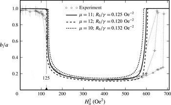
Axial ratio
 $b/a$
of equilibrium droplet shapes, in the plane of rotating field, as a function of the square of the field strength. Experimental data (circles) are compared with analytic calculations (black lines) using ellipsoidal approximation formula (2.22). The calculation with
 $\unicode[STIX]{x1D707}=11$
and
 $R_{0}/\unicode[STIX]{x1D6FE}=0.125~\text{Oe}^{-2}$
fits the best. Thin dashed lines indicate separate experiments. The critical field value, which is determined by relaxation of symmetry-destroying perturbations (see figure 11
b) is marked with a triangle at
 $H_{0}^{2}=125~\text{Oe}^{2}$
.

Both in numerical simulations and experiments we see that the oblate magnetic droplet becomes unstable with a respect to axial symmetry-breaking perturbations at the critical magnetic Bond number. Above the threshold value of the magnetic Bond number it assumes a worm-like shape for small fields and a star-like shape for larger magnetic Bond numbers, possibly by a bifurcation of a different kind (see figure 1). The droplets axial ratio
 $b/a$
obtained experimentally in the range of moderate field strength is shown in figure 10. Separate experiments, indicated with thin dashed lines, show a good agreement up to a field
 $H^{2}\approx 550~\text{Oe}^{2}$
. Above that, the droplet shape can remain elongated, but relaxes to the energetically more preferable star shape (as shown in § 4.2), if the deformation via the increase of the field is large enough.
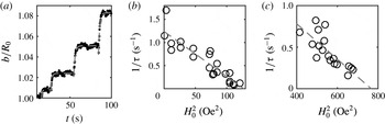
(a) Shape perturbations resulting from small stepwise field increases. For each step an exponential decay with a characteristic time
 $\unicode[STIX]{x1D70F}$
is observed. (b,c) Magnetic field dependence of the characteristic decay for symmetry-destroying perturbations: (b) approaching the oblate–prolate transition and (c) approaching the prolate–oblate transition. Dashed lines are best linear fits.

The magnetic field is increased by small steps. Nevertheless, as shown in figure 11(a) the shape perturbations and their dynamics (black dots) can be visually detected, which allows us to trace their characteristic decay time
 $\unicode[STIX]{x1D70F}$
(dashed line). As in the numerical simulation (see figure 8) the critical slowing down for the decay of perturbations in the case of an oblate shape is shown in figure 11(b). It leads to a critical field is
 $H_{c}^{2}=125~\text{Oe}^{2}$
. Experimentally it is possible to observe the critical slowing down of the prolate shape as shown in figure 11(c), when approaching the prolate–oblate transition, where the critical field is
 $H_{c,2}^{2}=765~\text{Oe}^{2}$
.
The compression of the oblate shape is determined from the semi-axes of the visible projection of the droplet approximated by a three-dimensional ellipsoid according to
 $c/R_{0}=R_{0}^{2}/ab$
. By numerical experimentation with formula (2.21) we have found that the semi-axial ratio
 $1/K$
is a linear function of
 $H_{0}^{2}$
in a broader field range than
 $c/R_{0}=K^{-2/3}$
. Thus from experiment we deduce
 $1/K=(ab/R_{0}^{2})^{-3/2}$
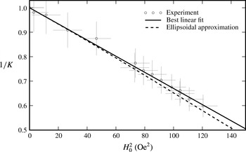
. In figure 12
 $1/K$
is plotted as a function of
 $H_{0}^{2}$
. It is adjusted with the relation
 $$\begin{eqnarray}\frac{1}{K}=1-\frac{H_{0}^{2}}{H_{\ast }^{2}},\end{eqnarray}$$
and
 $H_{\ast }^{2}=303~\text{Oe}^{2}$
. While according to (2.21)
 $H_{\ast }^{2}$
reads
 $$\begin{eqnarray}H_{\ast }^{2}=\frac{64\unicode[STIX]{x03C0}}{9}\left(\frac{\unicode[STIX]{x1D707}+2}{\unicode[STIX]{x1D707}-1}\right)^{2}\frac{\unicode[STIX]{x1D6FE}}{R_{0}}.\end{eqnarray}$$
In § 4 it is shown that the ellipsoidal approximation for the calculation of the axis ratio
 $b/a$
is valid even when the droplet becomes non-ellipsoidal. Thus we use the ellipsoid approximation to fit the data, adjusting
 $\unicode[STIX]{x1D707}$
with constrained
 $R_{0}/\unicode[STIX]{x1D6FE}$
by relation (5.5). In figure 10 we plot the ratio
 $b/a$
obtained analytically from the ellipsoidal approximation for
 $\unicode[STIX]{x1D707}=10,11,12$
. We see that theory gives a very good agreement when
 $\unicode[STIX]{x1D707}=11$
. This value also agrees with the elongation experiment we did in § 5.3.
Compression of the oblate shape in dependence on the square of field strength; experimental data (dots) calculated with formula
 $1/K=(ab/R_{0}^{2})^{-3/2}$
; best linear fit of the data (solid line); analytical calculation with ellipsoidal approximation (dashed line) with
 $\unicode[STIX]{x1D707}=11$
and
 $R_{0}/\unicode[STIX]{x1D6FE}=0.125~\text{Oe}^{-2}$
.

When we take
 $\unicode[STIX]{x1D707}=11$
and
 $R_{0}=10~\unicode[STIX]{x1D707}\text{m}$
, we get the surface tension from (5.5)
 $\unicode[STIX]{x1D6FE}=8.0\times 10^{-3}~\text{erg}/\text{cm}^{2}$
(
 $R_{0}/\unicode[STIX]{x1D6FE}=0.125~\text{Oe}^{-2}$
in reduced numerical unit). This value is slightly larger than the one calculated from the elongation experiment. But as we see in figure 10 that it fits better the axial ratio data. We take this value to evaluate magnetic Bond number in the rotating field experiments.
Another peculiar aspect, for which we can use the results obtained thus far, is for the calculation of the critical magnetic Bond number
 $Bm_{c}$
. According to figure 11 we have
 $H_{c}^{2}=125~\text{Oe}^{2}$
. This results in
 $Bm_{c}=15.6$
(
 $R_{0}/\unicode[STIX]{x1D6FE}=0.125~\text{Oe}^{-2}$
), which is close to the value obtained numerically
 $Bm_{c}=16.2$
. Since energy differences between the axial and triaxial shapes are very small near the critical magnetic Bond number then the deviation can either come from numerical errors or some small physical effects in experiments.
As the typical properties of the droplets are now determined we use in the following the magnetic Bond number
 $Bm$
to characterize the state of the droplet. The rich family of characteristic drop shapes observed during these experimental measurements is displayed in the introduction of this work (see figure 1).
5.5 Comparison of experimental and numerical results
We first compare qualitatively the equilibrium figures obtained experimentally with the numerical simulation results from § 4 in figure 13. Numerous effects can be seen in the experiments and in the simulations. (i) For magnetic Bond numbers under
 $Bm<20$
the droplet becomes flatter with increasing field strength as shown in figure 2 which is very well described with analytical results. Figure 12 shows that this droplet flattening
 $1/K=c/a=f(H_{0})$
is almost a linear function of field strength square. (ii) At
 $Bm_{c}=20$
, there is a spontaneous symmetry breaking. (iii) For
 $20<Bm<50$
, the worm-like shape elongation increases with the field strength. (iv) For
 $50<Bm<80$
a non-ellipsoidal regime where the droplet becomes wider, flatter and forms sharp tips is observed. (v) At
 $Bm=85$
a re-entrant transition is observed experimentally. We were not able to simulate it numerically since the droplet becomes so flat that it would need more than 10 000 triangles to have a width of at least three elements. It would require a very time consuming simulation.
Qualitative comparison of equilibrium figures obtained experimentally (a) and numerically (b). Experiments correspond to
 $\unicode[STIX]{x1D707}=11$
and
 $R_{0}/\unicode[STIX]{x1D6FE}=0.125~\text{Oe}^{-2}$
. Numerical simulation has
 $\unicode[STIX]{x1D707}=10$
. Black and white numbers on figures are magnetic Bond numbers.

To explore the star-like shapes we started with an already broken symmetry mesh and put corresponding magnetic field on. We obtained shapes qualitatively similar to the experimental star-like shapes (see figure 5). A more detailed investigation of hysteresis at the re-entrant transition is pending for a future publication. Here we only point out that its observation in numerical simulations is not easy due to the strong compression of the droplet at large magnetic Bond number values.
Comparison of shapes observed in experiment and in numerical simulations. The worm-like figure is obtained starting initially with an ellipsoid. The star is obtained starting from a seed, given by (4.2). To emphasize the differences and the similarities between experimental shapes and numerical ones, we plot as a white line the outline obtained from simulations on the two experimental images.
 $\unicode[STIX]{x1D707}=11$
and
 $R_{0}/\unicode[STIX]{x1D6FE}=0.125~\text{Oe}^{-2}$
.

As an important result we present a quantitative comparison of equilibrium figures obtained experimentally and numerically by drawing calculated equilibrium shapes on top of experimental images as shown in figure 14. Overall we see a good agreement except that simulation tips are a bit shorter either because of numerical errors or because
 $\unicode[STIX]{x1D707}$
is slightly larger in the experiment.
It is also worth noting the differences between experimental data and elliposoidal approximation at larger fields, as visible in figure 10 for
 $H^{2}>550$
. For this we see several possible explanations. First, the drop shape at larger fields is no more ellipsoidal, but takes a rather flattened shape with sharper tips. Second, the surface tension of the concentrated magnetic particle system might become anisotropic under large fields. Third, owing to different field increase steps, as visible in figure 10, perturbations of different magnitude are imposed on the droplet changing the value of field strength at which the re-entrant transition is observed.
6 Conclusions and discussion
As a general comment we would like to emphasize that the description of the highly magnetic droplets under study here, which are issued from a phase separation, is not obvious. These droplets are in fact based on a new kind of soft magnetic matter with strong interparticle interaction. We show here that many features of their under-field behaviour may be however described by a simple model of magnetic fluid. Moreover it is shown here that the boundary-integral equation technique allows one to develop efficient numerical algorithms for the simulation of the equilibrium shapes of these magnetic droplets submitted to an applied field either static or rotating. Numerical and experimental results show a good agreement at equilibrium and as well during shape relaxation processes. Under a rotating field, many similar features are observed both in numerical simulations and experiments, namely – instability of the axially symmetric droplet shape with respect to the symmetry-destroying perturbations (leading to the oblate–prolate transition), flattening of the prolate shape as the rotating magnetic field strength is increased, formation of the starfish-like equilibrium shapes.
The experimental and numerical results show that the behaviour of the magnetic droplets may be well described by approximating their shape by a triaxial ellipsoid. However the observed deviations from the simple ellipsoidal approximation, such as the formation of sharp tips, challenge for their theoretical description. Besides that, further development of this work is connected with accounting for the large viscosity contrast between the magnetic droplet and the surrounding fluid. This is possible by applying the boundary-integral equation technique to the solution of Stokes equation. Another important issue which should be mentioned with respect to these strongly magnetic droplets, issued from a phase separation, is the contribution of the magnetic dipolar interactions to their surface tension. An estimate shows that this contribution is of the same order of magnitude as the surface tension determined in experiments and it may depend on the orientation of the interface with respect to the applied field.
Acknowledgements
The authors are grateful to D. Talbot for providing us with the magnetic fluid sample and R. Livanovics for fruitful discussions. The research was funded by a project of the University of Latvia ‘Nano and quantum technologies, innovative materials – Soft materials in electromagnetic field’.
Appendix A. Boundary-integral equations
A.1 Boundary-integral equation for potential
For the potential boundary-integral equation derivation we are going to use formula (3.1) which follows from Green’s formula. With subscripts
 $\unicode[STIX]{x1D713}^{(i)}$
and
 $\unicode[STIX]{x1D713}^{(e)}$
we denote the limiting values of the potential approaching the surface from each side of the droplet boundary. For the limiting value from the inside we use relation (3.1) when
 $\boldsymbol{y}\in \unicode[STIX]{x2202}\unicode[STIX]{x1D6FA}$
 $$\begin{eqnarray}2\unicode[STIX]{x03C0}\unicode[STIX]{x1D713}^{(i)}(\boldsymbol{y})=\int _{\unicode[STIX]{x2202}\unicode[STIX]{x1D6FA}}\frac{\unicode[STIX]{x2202}\unicode[STIX]{x1D713}^{(i)}}{\unicode[STIX]{x2202}n_{\boldsymbol{x}}}\frac{1}{|\boldsymbol{x}-\boldsymbol{y}|}\,\text{d}S_{\boldsymbol{x}}-\unicode[STIX]{x2A0D}_{\unicode[STIX]{x2202}\unicode[STIX]{x1D6FA}}\unicode[STIX]{x1D713}^{(i)}(\boldsymbol{x})\frac{\unicode[STIX]{x2202}}{\unicode[STIX]{x2202}n_{\boldsymbol{x}}}\frac{1}{|\boldsymbol{x}-\boldsymbol{y}|}\,\text{d}S_{\boldsymbol{x}}\end{eqnarray}$$
and for the external region
 $\unicode[STIX]{x1D6FA}_{e}=\infty -\unicode[STIX]{x1D6FA}$
when
 $\boldsymbol{y}\in \unicode[STIX]{x2202}\unicode[STIX]{x1D6FA}$
 $$\begin{eqnarray}\displaystyle 2\unicode[STIX]{x03C0}\unicode[STIX]{x1D713}^{(e)}(\boldsymbol{y}) & = & \displaystyle -\int _{\unicode[STIX]{x2202}\unicode[STIX]{x1D6FA}}\frac{\unicode[STIX]{x2202}\unicode[STIX]{x1D713}^{(e)}}{\unicode[STIX]{x2202}n_{\boldsymbol{x}}}\frac{1}{|\boldsymbol{x}-\boldsymbol{y}|}\,\text{d}S_{\boldsymbol{x}}+\unicode[STIX]{x2A0D}_{\unicode[STIX]{x2202}\unicode[STIX]{x1D6FA}}\unicode[STIX]{x1D713}^{(e)}\frac{\unicode[STIX]{x2202}}{\unicode[STIX]{x2202}n_{\boldsymbol{x}}}\frac{1}{|\boldsymbol{x}-\boldsymbol{y}|}\,\text{d}S_{\boldsymbol{x}}\nonumber\\ \displaystyle & & \displaystyle +\,\int _{\unicode[STIX]{x2202}\infty }\frac{\unicode[STIX]{x2202}\unicode[STIX]{x1D713}}{\unicode[STIX]{x2202}n_{\boldsymbol{x}}}\frac{1}{|\boldsymbol{x}-\boldsymbol{y}|}\,\text{d}S_{\boldsymbol{x}}-\int _{\unicode[STIX]{x2202}\infty }\unicode[STIX]{x1D713}\frac{\unicode[STIX]{x2202}}{\unicode[STIX]{x2202}n_{\boldsymbol{x}}}\frac{1}{|\boldsymbol{x}-\boldsymbol{y}|}\,\text{d}S_{\boldsymbol{x}},\end{eqnarray}$$
where for the first two integrals we changed the direction of the normal vector so it is directed outwards of
 $\unicode[STIX]{x1D6FA}$
. The last two integrals of (A 2), according to (3.1), correspond to the external field contribution to the potential. Since here we are interested in case of homogenous field whose potential is
 $\boldsymbol{H}_{0}\boldsymbol{\cdot }\boldsymbol{y}$
then we rewrite (A 2)
 $$\begin{eqnarray}2\unicode[STIX]{x03C0}\unicode[STIX]{x1D713}^{(e)}(\boldsymbol{y})=4\unicode[STIX]{x03C0}\boldsymbol{H}_{0}\boldsymbol{\cdot }\boldsymbol{y}-\int _{\unicode[STIX]{x2202}\unicode[STIX]{x1D6FA}}\frac{\unicode[STIX]{x2202}\unicode[STIX]{x1D713}^{(e)}}{\unicode[STIX]{x2202}n_{\boldsymbol{x}}}\frac{1}{|\boldsymbol{x}-\boldsymbol{y}|}\,\text{d}S_{\boldsymbol{x}}+\unicode[STIX]{x2A0D}_{\unicode[STIX]{x2202}\unicode[STIX]{x1D6FA}}\unicode[STIX]{x1D713}^{(e)}\frac{\unicode[STIX]{x2202}}{\unicode[STIX]{x2202}n_{\boldsymbol{x}}}\frac{1}{|\boldsymbol{x}-\boldsymbol{y}|}\,\text{d}S_{\boldsymbol{x}}.\end{eqnarray}$$
Multiplying equation (A 1) by
 $\unicode[STIX]{x1D707}$
and adding it to (A 3) and using the boundary conditions
 $\unicode[STIX]{x1D713}^{(i)}=\unicode[STIX]{x1D713}^{(e)}$
and
 $(\unicode[STIX]{x2202}\unicode[STIX]{x1D713}^{(e)}/\unicode[STIX]{x2202}n)=\unicode[STIX]{x1D707}(\unicode[STIX]{x2202}\unicode[STIX]{x1D713}^{(i)}/\unicode[STIX]{x2202}n)$
we obtain the boundary-integral equation for the potential
 $$\begin{eqnarray}\unicode[STIX]{x1D713}(\boldsymbol{y})=\frac{2\boldsymbol{H}_{0}\boldsymbol{\cdot }\boldsymbol{y}}{\unicode[STIX]{x1D707}+1}-\frac{1}{2\unicode[STIX]{x03C0}}\frac{\unicode[STIX]{x1D707}-1}{\unicode[STIX]{x1D707}+1}\unicode[STIX]{x2A0D}_{\unicode[STIX]{x2202}\unicode[STIX]{x1D6FA}}\unicode[STIX]{x1D713}(\boldsymbol{x})\frac{\unicode[STIX]{x2202}}{\unicode[STIX]{x2202}n_{\boldsymbol{x}}}\frac{1}{|\boldsymbol{x}-\boldsymbol{y}|}\,\text{d}S_{\boldsymbol{x}},\end{eqnarray}$$
where we omit the suffixes since the potential is continuous.
A.2 Boundary-integral formula for normal component
Looking for the solution of the Laplace equation in the form of a single layer potential it is possible to derive the boundary-integral equation for the normal component of the magnetic field strength. Numerical calculations showed that the solution of this equation is ill behaved and so we have chosen an alternative approach deriving an integral relation which allows us to calculate the normal component of the magnetic field strength from the known tangential component.
Let us consider the identity
 $$\begin{eqnarray}\unicode[STIX]{x1D735}_{\boldsymbol{x}}\boldsymbol{\cdot }(\boldsymbol{Q}\times \boldsymbol{B})=\boldsymbol{B}\boldsymbol{\cdot }\unicode[STIX]{x1D735}_{\boldsymbol{x}}\times \boldsymbol{Q},\end{eqnarray}$$
where
 $\boldsymbol{B}$
is the magnetic induction,
 $\boldsymbol{Q}=\unicode[STIX]{x1D735}_{\boldsymbol{x}}\times \boldsymbol{a}/|\boldsymbol{x}-\boldsymbol{y}|$
(
 $\boldsymbol{a}$
is an arbitrary constant vector). It is easy to check that
 $\unicode[STIX]{x1D735}_{\boldsymbol{x}}\times \boldsymbol{Q}=(\boldsymbol{a}\boldsymbol{\cdot }\unicode[STIX]{x1D735}_{\boldsymbol{x}})\unicode[STIX]{x1D735}_{\boldsymbol{x}}1/|\boldsymbol{x}-\boldsymbol{y}|$
. Integrating relation (A 5) throughout the arbitrary region
 $\unicode[STIX]{x1D6FA}$
in dependence on the position of the point with the radius vector
 $\boldsymbol{y}$
we have
 $$\begin{eqnarray}\int _{\unicode[STIX]{x2202}\unicode[STIX]{x1D6FA}}(\boldsymbol{B}\times \boldsymbol{n}_{\boldsymbol{x}})\times \unicode[STIX]{x1D735}_{\boldsymbol{x}}\frac{1}{|\boldsymbol{x}-\boldsymbol{y}|}\,\text{d}S_{\boldsymbol{x}}-\int _{\unicode[STIX]{x2202}\unicode[STIX]{x1D6FA}}(\boldsymbol{B}\boldsymbol{\cdot }\boldsymbol{n}_{\boldsymbol{x}})\unicode[STIX]{x1D735}_{\boldsymbol{x}}\frac{1}{|\boldsymbol{x}-\boldsymbol{y}|}\,\text{d}S_{\boldsymbol{x}}=\left\{\begin{array}{@{}ll@{}}4\unicode[STIX]{x03C0}\boldsymbol{B}(\boldsymbol{y}) & \text{if }\boldsymbol{y}\in \unicode[STIX]{x1D6FA}\\ 2\unicode[STIX]{x03C0}\boldsymbol{B}(\boldsymbol{y}) & \text{if }\boldsymbol{y}\in \unicode[STIX]{x2202}\unicode[STIX]{x1D6FA}\\ 0 & \text{if }\boldsymbol{y}\in \overline{\unicode[STIX]{x1D6FA}\cup \unicode[STIX]{x2202}\unicode[STIX]{x1D6FA}},\end{array}\right.\end{eqnarray}$$
where
 $\boldsymbol{n}$
is the external normal to the boundary of the region and the integrals in the case
 $\boldsymbol{y}\in \unicode[STIX]{x2202}\unicode[STIX]{x1D6FA}$
are taken as the Cauchy principal value integrals.
Applying relation (A 6) for the region
 $\unicode[STIX]{x1D6FA}_{e}=\infty -\unicode[STIX]{x1D6FA}$
, where
 $\unicode[STIX]{x1D6FA}$
is the region occupied by the magnetic droplet at
 $\boldsymbol{y}\in \unicode[STIX]{x2202}\unicode[STIX]{x1D6FA}$
we have (at
 $\unicode[STIX]{x2202}\unicode[STIX]{x1D6FA}$
we take
 $\boldsymbol{n}$
as the external normal to the surface of the droplet)
 $$\begin{eqnarray}\displaystyle 2\unicode[STIX]{x03C0}\boldsymbol{B}^{(e)}(\boldsymbol{y}) & = & \displaystyle -\unicode[STIX]{x2A0D}_{\unicode[STIX]{x2202}\unicode[STIX]{x1D6FA}}[\boldsymbol{B}^{(e)}\times \boldsymbol{n}_{\boldsymbol{x}}]\times \unicode[STIX]{x1D735}_{\boldsymbol{x}}\frac{1}{|\boldsymbol{x}-\boldsymbol{y}|}\,\text{d}S_{\boldsymbol{x}}+\unicode[STIX]{x2A0D}_{\unicode[STIX]{x2202}\unicode[STIX]{x1D6FA}}(\boldsymbol{B}^{(e)}\boldsymbol{\cdot }\boldsymbol{n}_{\boldsymbol{ x}})\unicode[STIX]{x1D735}_{\boldsymbol{x}}\frac{1}{|\boldsymbol{x}-\boldsymbol{y}|}\,\text{d}S_{\boldsymbol{x}}\nonumber\\ \displaystyle & & \displaystyle +\,\int _{\unicode[STIX]{x2202}\infty }(\boldsymbol{B}\times \boldsymbol{n}_{\boldsymbol{x}})\times \unicode[STIX]{x1D735}_{\boldsymbol{x}}\frac{1}{|\boldsymbol{x}-\boldsymbol{y}|}\,\text{d}S_{\boldsymbol{x}}-\int _{\unicode[STIX]{x2202}\infty }(\boldsymbol{B}\boldsymbol{\cdot }\boldsymbol{n}_{\boldsymbol{x}})\unicode[STIX]{x1D735}_{\boldsymbol{x}}\frac{1}{|\boldsymbol{x}-\boldsymbol{y}|}\,\text{d}S_{\boldsymbol{x}}.\end{eqnarray}$$
According to relation (A 5) the last two integrals correspond to the contribution of the external field. Since we have a homogeneous field
 $\boldsymbol{H}_{0}$
(without droplet) everywhere then we rewrite relation (A 7) as
 $$\begin{eqnarray}2\unicode[STIX]{x03C0}\boldsymbol{B}^{(e)}=-\unicode[STIX]{x2A0D}_{\unicode[STIX]{x2202}\unicode[STIX]{x1D6FA}}(\boldsymbol{B}^{(e)}\times \boldsymbol{n}_{\boldsymbol{ x}})\times \unicode[STIX]{x1D735}_{\boldsymbol{x}}\frac{1}{|\boldsymbol{x}-\boldsymbol{y}|}\,\text{d}S_{\boldsymbol{x}}+\unicode[STIX]{x2A0D}_{\unicode[STIX]{x2202}\unicode[STIX]{x1D6FA}}(\boldsymbol{B}^{(e)}\boldsymbol{\cdot }\boldsymbol{n}_{\boldsymbol{ x}})\unicode[STIX]{x1D735}_{\boldsymbol{x}}\frac{1}{|\boldsymbol{x}-\boldsymbol{y}|}\,\text{d}S_{\boldsymbol{x}}+4\unicode[STIX]{x03C0}\boldsymbol{H}_{0},\end{eqnarray}$$
where for simplicity we can say that
 $\boldsymbol{H}_{0}$
corresponds also to magnetic field far away from the droplet.
Taking the projection of relation (A 6) at
 $\boldsymbol{y}\in \unicode[STIX]{x2202}\unicode[STIX]{x1D6FA}$
and (A 8) on the normal to the interface and accounting for the boundary conditions
 $\boldsymbol{B}^{(e)}\boldsymbol{\cdot }\boldsymbol{n}=\boldsymbol{B}^{(i)}\boldsymbol{\cdot }\boldsymbol{n}$
and
 $\boldsymbol{H}^{(i)}\times \boldsymbol{n}=\boldsymbol{H}^{(e)}\times \boldsymbol{n}$
we obtain the following relation for the calculation of the normal component of the magnetic field
 $$\begin{eqnarray}\displaystyle \boldsymbol{B}\boldsymbol{\cdot }\boldsymbol{n}_{\boldsymbol{y}}=\boldsymbol{H}_{0}\boldsymbol{\cdot }\boldsymbol{n}_{\boldsymbol{y}}-\frac{\unicode[STIX]{x1D707}-1}{4\unicode[STIX]{x03C0}}\boldsymbol{n}_{\boldsymbol{y}}\boldsymbol{\cdot }\int _{\unicode[STIX]{x2202}\unicode[STIX]{x1D6FA}}(\boldsymbol{n}_{\boldsymbol{x}}\times \boldsymbol{H})\times \unicode[STIX]{x1D735}_{\boldsymbol{x}}\frac{1}{|\boldsymbol{x}-\boldsymbol{y}|}\,\text{d}S_{\boldsymbol{x}}. & & \displaystyle\end{eqnarray}$$
A.3 Boundary-integral equation for normal component of field
While we had a lack of success with direct calculation of the normal field with the boundary-integral equation in our studies, we have derived a corresponding equation for three dimensions. Here we briefly give the derivation as it is analogous and uses previous results of derivations (A 4) and (A 9).
Again taking the normal projection of relation (A 6) at
 $\boldsymbol{y}\in \unicode[STIX]{x2202}\unicode[STIX]{x1D6FA}$
and (A 8) and using the boundary conditions
 $\boldsymbol{B}^{(e)}\boldsymbol{\cdot }\boldsymbol{n}=\boldsymbol{B}^{(i)}\boldsymbol{\cdot }\boldsymbol{n}$
and
 $\boldsymbol{H}^{(i)}\times \boldsymbol{n}=\boldsymbol{H}^{(e)}\times \boldsymbol{n}$
we subtract
 $\int _{\unicode[STIX]{x2202}\unicode[STIX]{x1D6FA}}(\boldsymbol{B}\times \boldsymbol{n}_{\boldsymbol{x}})\times \unicode[STIX]{x1D735}_{\boldsymbol{x}}1/|\boldsymbol{x}-\boldsymbol{y}|\,\text{d}S_{\boldsymbol{x}}$
and obtain
 $$\begin{eqnarray}B_{n}(\boldsymbol{y})=\frac{2\unicode[STIX]{x1D707}\boldsymbol{H}_{0}\boldsymbol{\cdot }\boldsymbol{n}_{\boldsymbol{y}}}{\unicode[STIX]{x1D707}+1}+\frac{1}{2\unicode[STIX]{x03C0}}\frac{\unicode[STIX]{x1D707}-1}{\unicode[STIX]{x1D707}+1}\unicode[STIX]{x2A0D}_{\unicode[STIX]{x2202}\unicode[STIX]{x1D6FA}}B_{n}(\boldsymbol{x})\frac{\unicode[STIX]{x2202}}{\unicode[STIX]{x2202}n_{\boldsymbol{y}}}\frac{1}{|\boldsymbol{x}-\boldsymbol{y}|}\,\text{d}S_{\boldsymbol{x}},\end{eqnarray}$$
where
 $B_{n}=\boldsymbol{B}\boldsymbol{\cdot }\boldsymbol{n}$
. This equation is remarkably similar to the boundary-integral equation for potential (A 4) except for normal derivative inside the integral. Using the same numerical procedure as outlined in § 3 (plane triangles, trapezoidal integration for all triangles) we report that this integral equation gives large errors. This is clearly because we do not integrate the singular quadrature properly which is cumbersome for three dimensions.
Appendix B. Singularity subtraction
Consider identity with
 $\boldsymbol{y}\ni \unicode[STIX]{x1D6FA}$
 $$\begin{eqnarray}\int _{\unicode[STIX]{x2202}\unicode[STIX]{x1D6FA}}\boldsymbol{n}_{\boldsymbol{x}}\boldsymbol{\cdot }\unicode[STIX]{x1D735}_{\boldsymbol{x}}\frac{1}{|\boldsymbol{x}-\boldsymbol{y}|}\,\text{d}S_{\boldsymbol{x}}=0,\end{eqnarray}$$
which can easily be proven with the divergence theorem and using
 $\unicode[STIX]{x1D6E5}_{\boldsymbol{x}}1/|\boldsymbol{x}-\boldsymbol{y}|=0$
. For taking the limit
 $\boldsymbol{y}\rightarrow \unicode[STIX]{x2202}\unicode[STIX]{x1D6FA}$
we will split the integration domain into two parts. One integral is for all surface except for the excluded region with a radius
 $\unicode[STIX]{x1D700}$
centred at
 $\boldsymbol{y}$
which in the limit
 $\unicode[STIX]{x1D700}\rightarrow 0$
gives us a principal value integral. The other one is around the half-sphere whose value can be calculated analytically
 $$\begin{eqnarray}\int _{\unicode[STIX]{x2202}\unicode[STIX]{x1D6FA}_{\unicode[STIX]{x1D700}}}\boldsymbol{n}_{\boldsymbol{x}}\boldsymbol{\cdot }\unicode[STIX]{x1D735}_{\boldsymbol{x}}\frac{1}{|\boldsymbol{x}-\boldsymbol{y}|}\,\text{d}S_{\boldsymbol{x}}=\int _{\unicode[STIX]{x2202}\unicode[STIX]{x1D6FA}_{\unicode[STIX]{x1D700}}}\frac{1}{|\boldsymbol{x}-\boldsymbol{y}|^{2}}\,\text{d}S_{\boldsymbol{x}}=2\unicode[STIX]{x03C0}\int _{\unicode[STIX]{x03C0}/2}^{\unicode[STIX]{x03C0}}\sin \unicode[STIX]{x1D703}\,\text{d}\unicode[STIX]{x1D703}=2\unicode[STIX]{x03C0}.\end{eqnarray}$$
Taking the limit
 $\unicode[STIX]{x1D700}\rightarrow 0$
we conclude that limiting value of the integral (B 1) is
 $$\begin{eqnarray}\unicode[STIX]{x2A0D}_{\unicode[STIX]{x2202}\unicode[STIX]{x1D6FA}}\boldsymbol{n}_{\boldsymbol{x}}\boldsymbol{\cdot }\unicode[STIX]{x1D735}_{\boldsymbol{x}}\frac{1}{|\boldsymbol{x}-\boldsymbol{y}|}\,\text{d}S_{\boldsymbol{x}}=\int _{\unicode[STIX]{x2202}\unicode[STIX]{x1D6FA}}-\int _{\unicode[STIX]{x2202}\unicode[STIX]{x1D6FA}_{\unicode[STIX]{x1D700}}}=-2\unicode[STIX]{x03C0},\end{eqnarray}$$
which we use for the singularity subtraction in (3.4).
When
 $\boldsymbol{y}\ni \unicode[STIX]{x1D6FA}$
we have another identity
 $$\begin{eqnarray}\int _{\unicode[STIX]{x2202}\unicode[STIX]{x1D6FA}}\boldsymbol{n}_{\boldsymbol{x}}\times \unicode[STIX]{x1D735}_{\boldsymbol{x}}\frac{1}{|\boldsymbol{x}-\boldsymbol{y}|}\,\text{d}S_{\boldsymbol{x}}=\int _{\unicode[STIX]{x1D6FA}}\unicode[STIX]{x1D735}_{\boldsymbol{x}}\times \unicode[STIX]{x1D735}_{\boldsymbol{x}}\frac{1}{|\boldsymbol{x}-\boldsymbol{y}|}\,\text{d}V_{\boldsymbol{x}}=0\end{eqnarray}$$
since the curl of a potential field is
 $0$
. For taking the limit
 $\boldsymbol{y}\rightarrow \boldsymbol{x}$
we again split the integration domain into two parts. Integral around the half-sphere is
 $0$
as the normal vector
 $\boldsymbol{n}_{\boldsymbol{x}}$
is collinear with
 $\unicode[STIX]{x1D735}_{\boldsymbol{x}}1/|\boldsymbol{x}-\boldsymbol{y}|$
when
 $\boldsymbol{y}$
is at the centre of the half-sphere. So we conclude that the principal value integral when
 $\boldsymbol{y}\in \unicode[STIX]{x2202}\unicode[STIX]{x1D6FA}$
is
 $$\begin{eqnarray}\unicode[STIX]{x2A0D}_{\unicode[STIX]{x2202}\unicode[STIX]{x1D6FA}}\boldsymbol{n}_{\boldsymbol{x}}\times \unicode[STIX]{x1D735}_{\boldsymbol{x}}\frac{1}{|\boldsymbol{x}-\boldsymbol{y}|}\,\text{d}S_{\boldsymbol{x}}=0.\end{eqnarray}$$
For deriving the formula used in (3.9) we start with the identity
 $$\begin{eqnarray}\boldsymbol{A}\times (\boldsymbol{B}\times \boldsymbol{C})=\boldsymbol{A}(\boldsymbol{B}\boldsymbol{\cdot }\boldsymbol{C})-\boldsymbol{C}(\boldsymbol{A}\boldsymbol{\cdot }\boldsymbol{B})+\boldsymbol{C}\times (\boldsymbol{B}\times \boldsymbol{A}).\end{eqnarray}$$
Putting
 $\boldsymbol{A}\rightarrow \unicode[STIX]{x1D735}_{\boldsymbol{x}}1/|\boldsymbol{x}-\boldsymbol{y}|$
,
 $\boldsymbol{B}\rightarrow \boldsymbol{n}_{\boldsymbol{x}}$
,
 $\boldsymbol{C}\rightarrow P\boldsymbol{H}_{\boldsymbol{x}}$
gives us the following integral identity
 $$\begin{eqnarray}\displaystyle \unicode[STIX]{x2A0D}_{\unicode[STIX]{x2202}\unicode[STIX]{x1D6FA}}\unicode[STIX]{x1D735}_{\boldsymbol{x}}\frac{1}{|\boldsymbol{x}-\boldsymbol{y}|}\times (\boldsymbol{n}_{\boldsymbol{x}}\times \boldsymbol{H}_{\boldsymbol{x}})\,\text{d}S_{\boldsymbol{x}} & = & \displaystyle \unicode[STIX]{x2A0D}_{\unicode[STIX]{x2202}\unicode[STIX]{x1D6FA}}P\boldsymbol{H}_{\boldsymbol{x}}\times (\boldsymbol{n}_{\boldsymbol{x}}\times \unicode[STIX]{x1D735}_{\boldsymbol{x}}\frac{1}{|\boldsymbol{x}-\boldsymbol{y}|})\,\text{d}S_{\boldsymbol{x}}\nonumber\\ \displaystyle & & \displaystyle -\,\unicode[STIX]{x2A0D}_{\unicode[STIX]{x2202}\unicode[STIX]{x1D6FA}}P\boldsymbol{H}_{\boldsymbol{x}}\left(\boldsymbol{n}_{\boldsymbol{x}}\boldsymbol{\cdot }\unicode[STIX]{x1D735}_{\boldsymbol{x}}\frac{1}{|\boldsymbol{x}-\boldsymbol{y}|}\right)\text{d}S_{\boldsymbol{x}}.\end{eqnarray}$$
Using the singularity subtraction identities (B 5) and (B 3) for both integrals on the right-hand side we obtain
 $$\begin{eqnarray}\displaystyle \unicode[STIX]{x2A0D}_{\unicode[STIX]{x2202}\unicode[STIX]{x1D6FA}}\unicode[STIX]{x1D735}_{\boldsymbol{x}}\frac{1}{|\boldsymbol{x}-\boldsymbol{y}|}\times (\boldsymbol{n}_{\boldsymbol{x}}\times \boldsymbol{H}_{\boldsymbol{x}})\,\text{d}S_{\boldsymbol{x}}=\unicode[STIX]{x2A0D}_{\unicode[STIX]{x2202}\unicode[STIX]{x1D6FA}}(P\boldsymbol{H}_{\boldsymbol{x}}-P\boldsymbol{H}_{\boldsymbol{y}})\times (\boldsymbol{n}_{\boldsymbol{x}}\times \unicode[STIX]{x1D735}_{\boldsymbol{x}}\frac{1}{|\boldsymbol{x}-\boldsymbol{y}|})\,\text{d}S_{\boldsymbol{x}} & & \displaystyle \nonumber\\ \displaystyle -\unicode[STIX]{x2A0D}_{\unicode[STIX]{x2202}\unicode[STIX]{x1D6FA}}(P\boldsymbol{H}_{\boldsymbol{x}}-P\boldsymbol{H}_{\boldsymbol{y}})\left(\boldsymbol{n}_{\boldsymbol{x}}\boldsymbol{\cdot }\unicode[STIX]{x1D735}_{\boldsymbol{x}}\frac{1}{|\boldsymbol{x}-\boldsymbol{y}|}\right)\text{d}S_{\boldsymbol{x}}-2\unicode[STIX]{x03C0}P\boldsymbol{H}_{\boldsymbol{y}}. & & \displaystyle\end{eqnarray}$$
The right-hand side is now weakly singular and thus can be calculated by means of trapezoidal quadrature for a non-singular integral and using a transformation of variables for weakly singular elements.
Appendix C. Identity
To transform the integral
 $$\begin{eqnarray}\int \unicode[STIX]{x1D735}_{\boldsymbol{x}}\boldsymbol{\cdot }\left(\frac{\boldsymbol{n}_{\boldsymbol{x}}}{|\boldsymbol{y}-\boldsymbol{x}|}+\frac{(\boldsymbol{y}-\boldsymbol{x})(\boldsymbol{n}_{\boldsymbol{x}}\boldsymbol{\cdot }(\boldsymbol{y}-\boldsymbol{x}))}{|\boldsymbol{y}-\boldsymbol{x}|^{3}}\right)\text{d}S_{\boldsymbol{x}}\end{eqnarray}$$
we consider the two terms in (C 1) separately.
 $$\begin{eqnarray}\boldsymbol{I}^{(1)}=\int \frac{\unicode[STIX]{x1D735}_{\boldsymbol{x}}\boldsymbol{\cdot }\boldsymbol{n}_{\boldsymbol{x}}}{|\boldsymbol{y}-\boldsymbol{x}|}\,\text{d}S_{\boldsymbol{x}}.\end{eqnarray}$$
Multiplying (C 2) by an arbitrary constant vector
 $\boldsymbol{a}$
and using the relation
 $$\begin{eqnarray}\boldsymbol{a}\unicode[STIX]{x1D735}\boldsymbol{\cdot }\boldsymbol{n}=\unicode[STIX]{x1D735}\times [\boldsymbol{a}\times \boldsymbol{n}]+(\boldsymbol{a}\boldsymbol{\cdot }\unicode[STIX]{x1D735})\boldsymbol{n}\end{eqnarray}$$
we have
 $$\begin{eqnarray}\boldsymbol{a}\boldsymbol{\cdot }\boldsymbol{I}^{(1)}=\int \frac{\boldsymbol{n}_{\boldsymbol{x}}\boldsymbol{\cdot }\unicode[STIX]{x1D735}_{\boldsymbol{x}}\times [\boldsymbol{a}\times \boldsymbol{n}_{\boldsymbol{x}}]}{|\boldsymbol{y}-\boldsymbol{x}|}\,\text{d}S_{\boldsymbol{x}}+\int \frac{\boldsymbol{n}_{\boldsymbol{x}}\boldsymbol{\cdot }(\boldsymbol{a}\boldsymbol{\cdot }\unicode[STIX]{x1D735}_{\boldsymbol{x}})\boldsymbol{n}_{\boldsymbol{x}}}{|\boldsymbol{y}-\boldsymbol{x}|}\,\text{d}S_{\boldsymbol{x}}.\end{eqnarray}$$
Last term on the right-hand side of (C 4) is zero since
 $$\begin{eqnarray}\boldsymbol{n}\boldsymbol{\cdot }(\boldsymbol{a}\boldsymbol{\cdot }\unicode[STIX]{x1D735})\boldsymbol{n}={\textstyle \frac{1}{2}}(\boldsymbol{a}\boldsymbol{\cdot }\unicode[STIX]{x1D735})\boldsymbol{n}^{2}=0.\end{eqnarray}$$
The first term on the right-hand side is transformed as follows
 $$\begin{eqnarray}\displaystyle & & \displaystyle \int \frac{\boldsymbol{n}_{\boldsymbol{x}}\boldsymbol{\cdot }\unicode[STIX]{x1D735}_{\boldsymbol{x}}\times [\boldsymbol{a}\times \boldsymbol{n}_{\boldsymbol{x}}]}{|\boldsymbol{y}-\boldsymbol{x}|}\,\text{d}S_{\boldsymbol{x}}=\int \boldsymbol{n}_{\boldsymbol{x}}\boldsymbol{\cdot }\unicode[STIX]{x1D735}_{\boldsymbol{x}}\times \left[\frac{\boldsymbol{a}\times \boldsymbol{n}_{\boldsymbol{x}}}{|\boldsymbol{y}-\boldsymbol{x}|}\right]\,\text{d}S_{\boldsymbol{x}}\nonumber\\ \displaystyle & & \displaystyle \qquad -\,\int \boldsymbol{n}_{\boldsymbol{x}}\boldsymbol{\cdot }\left[\unicode[STIX]{x1D735}_{\boldsymbol{x}}\frac{1}{|\boldsymbol{y}-\boldsymbol{x}|}\times [\boldsymbol{a}\times \boldsymbol{n}_{\boldsymbol{x}}]\right]\,\text{d}S_{\boldsymbol{x}}.\end{eqnarray}$$
The first term on the right-hand side of relation (C 6) is zero since the integration is carried out over a closed surface. Since the vector
 $\boldsymbol{a}$
is arbitrary we obtain
 $$\begin{eqnarray}\boldsymbol{I}^{(1)}=-\int \boldsymbol{n}_{\boldsymbol{ x}}(\unicode[STIX]{x1D735}_{\boldsymbol{x}}\frac{1}{|\boldsymbol{y}-\boldsymbol{x}|}\boldsymbol{\cdot }\boldsymbol{n}_{\boldsymbol{x}})\,\text{d}S_{\boldsymbol{x}}+\int \frac{(\boldsymbol{y}-\boldsymbol{x})}{|\boldsymbol{y}-\boldsymbol{x}|^{3}}\,\text{d}S_{\boldsymbol{x}}.\end{eqnarray}$$
The second term in (C 1) is transformed similarly
 $$\begin{eqnarray}\displaystyle & \displaystyle \boldsymbol{I}^{(2)}=\int \unicode[STIX]{x1D735}_{\boldsymbol{x}}\boldsymbol{\cdot }\boldsymbol{n}_{\boldsymbol{x}}\frac{(\boldsymbol{y}-\boldsymbol{x})(\boldsymbol{n}_{\boldsymbol{x}}\boldsymbol{\cdot }(\boldsymbol{y}-\boldsymbol{x}))}{|\boldsymbol{y}-\boldsymbol{x}|^{3}}\,\text{d}S_{\boldsymbol{x}}; & \displaystyle\end{eqnarray}$$
 $$\begin{eqnarray}\displaystyle & \displaystyle \boldsymbol{a}\boldsymbol{\cdot }\boldsymbol{I}^{(2)}=\int \unicode[STIX]{x1D735}_{\boldsymbol{x}}\boldsymbol{\cdot }\boldsymbol{n}_{\boldsymbol{x}}\frac{\boldsymbol{a}\boldsymbol{\cdot }(\boldsymbol{y}-\boldsymbol{x})(\boldsymbol{n}_{\boldsymbol{x}}\boldsymbol{\cdot }(\boldsymbol{y}-\boldsymbol{x}))}{|\boldsymbol{y}-\boldsymbol{x}|^{3}}\,\text{d}S_{\boldsymbol{x}}. & \displaystyle\end{eqnarray}$$
Using the relation
 $$\begin{eqnarray}\boldsymbol{n}_{\boldsymbol{x}}\boldsymbol{\cdot }(\boldsymbol{y}-\boldsymbol{x})\unicode[STIX]{x1D735}_{\boldsymbol{x}}\boldsymbol{\cdot }\boldsymbol{n}_{\boldsymbol{x}}=-2+\boldsymbol{n}_{\boldsymbol{x}}\boldsymbol{\cdot }\unicode[STIX]{x1D735}_{\boldsymbol{x}}\times [(\boldsymbol{y}-\boldsymbol{x})\times \boldsymbol{n}_{\boldsymbol{x}}]\end{eqnarray}$$
we obtain
 $$\begin{eqnarray}\boldsymbol{a}\boldsymbol{\cdot }\boldsymbol{I}^{(2)}=\int \frac{\boldsymbol{a}\boldsymbol{\cdot }(\boldsymbol{y}-\boldsymbol{x})}{|\boldsymbol{y}-\boldsymbol{x}|^{3}}\boldsymbol{n}_{\boldsymbol{x}}\boldsymbol{\cdot }\unicode[STIX]{x1D735}_{\boldsymbol{x}}\times [(\boldsymbol{y}-\boldsymbol{x})\times \boldsymbol{n}_{\boldsymbol{x}}]\,\text{d}S_{\boldsymbol{x}}-2\int \frac{\boldsymbol{a}\boldsymbol{\cdot }(\boldsymbol{y}-\boldsymbol{x})}{|\boldsymbol{y}-\boldsymbol{x}|^{3}}\,\text{d}S_{\boldsymbol{x}}.\end{eqnarray}$$
The first term on the right-hand side of (C 11) may be transformed as follows
 $$\begin{eqnarray}\int \boldsymbol{n}_{\boldsymbol{x}}\boldsymbol{\cdot }\unicode[STIX]{x1D735}_{\boldsymbol{x}}\times \left[\frac{\boldsymbol{a}\boldsymbol{\cdot }(\boldsymbol{y}-\boldsymbol{x})}{|\boldsymbol{y}-\boldsymbol{x}|^{3}}(\boldsymbol{y}-\boldsymbol{x})\times \boldsymbol{n}_{\boldsymbol{x}}\right]\,\text{d}S_{\boldsymbol{x}}-\int \boldsymbol{n}_{\boldsymbol{x}}\boldsymbol{\cdot }\unicode[STIX]{x1D735}_{\boldsymbol{x}}\left[\frac{\boldsymbol{a}\boldsymbol{\cdot }(\boldsymbol{y}-\boldsymbol{x})}{|\boldsymbol{y}-\boldsymbol{x}|^{3}}\times [(\boldsymbol{y}-\boldsymbol{x})\times \boldsymbol{n}_{\boldsymbol{x}}]\right]\,\text{d}S_{\boldsymbol{x}}\end{eqnarray}$$
The first term on the right-hand side of relation (C 12) is zero since the integration is carried out over the closed surface. The second term on the right-hand side of relation (C 12) equals
 $$\begin{eqnarray}\frac{\boldsymbol{n}_{\boldsymbol{x}}\boldsymbol{\cdot }(\boldsymbol{y}-\boldsymbol{x})\boldsymbol{a}\boldsymbol{\cdot }\boldsymbol{n}_{\boldsymbol{x}}}{|\boldsymbol{y}-\boldsymbol{x}|^{3}}+2\frac{\boldsymbol{a}\boldsymbol{\cdot }(\boldsymbol{y}-\boldsymbol{x})}{|\boldsymbol{y}-\boldsymbol{x}|^{3}}-3\frac{\boldsymbol{a}\boldsymbol{\cdot }(\boldsymbol{y}-\boldsymbol{x})(\boldsymbol{n}_{\boldsymbol{x}}\boldsymbol{\cdot }(\boldsymbol{y}-\boldsymbol{x}))^{2}}{|\boldsymbol{y}-\boldsymbol{x}|^{5}}.\end{eqnarray}$$
As a result for
 $\boldsymbol{I}$
we have
 $$\begin{eqnarray}\boldsymbol{I}=\boldsymbol{I}^{(1)}+\boldsymbol{I}^{(2)}=\int \frac{\boldsymbol{y}-\boldsymbol{x}}{|\boldsymbol{y}-\boldsymbol{x}|^{3}}\,\text{d}S_{\boldsymbol{x}}-3\int \frac{(\boldsymbol{y}-\boldsymbol{x})(\boldsymbol{n}_{\boldsymbol{x}}\boldsymbol{\cdot }(\boldsymbol{y}-\boldsymbol{x}))^{2}}{|\boldsymbol{y}-\boldsymbol{x}|^{5}}\,\text{d}S_{\boldsymbol{x}}.\end{eqnarray}$$
 $$\begin{eqnarray}\displaystyle & & \displaystyle \frac{\boldsymbol{n}_{\boldsymbol{y}}\boldsymbol{\cdot }(\boldsymbol{y}-\boldsymbol{x})}{|\boldsymbol{y}-\boldsymbol{x}|^{3}}-3\frac{((\boldsymbol{y}-\boldsymbol{x})\boldsymbol{\cdot }\boldsymbol{n}_{\boldsymbol{x}})^{2}\boldsymbol{n}_{\boldsymbol{ y}}\boldsymbol{\cdot }(\boldsymbol{y}-\boldsymbol{x})}{|\boldsymbol{y}-\boldsymbol{x}|^{5}}\nonumber\\ \displaystyle & & \displaystyle \qquad -\,\frac{(\boldsymbol{y}-\boldsymbol{x})\boldsymbol{\cdot }(\boldsymbol{n}_{\boldsymbol{x}}+\boldsymbol{n}_{\boldsymbol{y}})}{|\boldsymbol{y}-\boldsymbol{x}|^{3}}\left(1-3\frac{(\boldsymbol{y}-\boldsymbol{x})\boldsymbol{\cdot }\boldsymbol{n}_{\boldsymbol{x}}(\boldsymbol{y}-\boldsymbol{x})\boldsymbol{\cdot }\boldsymbol{n}_{\boldsymbol{y}}}{|\boldsymbol{y}-\boldsymbol{x}|^{2}}\right)\nonumber\\ \displaystyle & & \displaystyle \quad =-\frac{(\boldsymbol{y}-\boldsymbol{x})\boldsymbol{\cdot }\boldsymbol{n}_{\boldsymbol{x}}}{|\boldsymbol{y}-\boldsymbol{x}|^{3}}+3\frac{(\boldsymbol{y}-\boldsymbol{x})\boldsymbol{\cdot }\boldsymbol{n}_{\boldsymbol{x}}(\boldsymbol{n}_{\boldsymbol{y}}\boldsymbol{\cdot }(\boldsymbol{y}-\boldsymbol{x}))^{2}}{|\boldsymbol{y}-\boldsymbol{x}|^{5}}.\end{eqnarray}$$
Since the integral of the right-hand side equals zero we arrive at the identity used in the text
 $$\begin{eqnarray}\displaystyle & & \displaystyle \boldsymbol{n}_{\boldsymbol{y}}\int \left(\frac{1}{R_{1}}+\frac{1}{R_{2}}\right)\left(\frac{\boldsymbol{n}_{\boldsymbol{x}}}{|\boldsymbol{y}-\boldsymbol{x}|}+\frac{(\boldsymbol{y}-\boldsymbol{x})(\boldsymbol{y}-\boldsymbol{x})\boldsymbol{\cdot }\boldsymbol{n}_{\boldsymbol{x}}}{|\boldsymbol{y}-\boldsymbol{x}|^{3}}\right)\text{d}S_{\boldsymbol{x}}\nonumber\\ \displaystyle & & \displaystyle \quad =\int \frac{(\boldsymbol{y}-\boldsymbol{x})(\boldsymbol{n}_{\boldsymbol{x}}+\boldsymbol{n}_{\boldsymbol{y}})}{|\boldsymbol{y}-\boldsymbol{x}|^{3}}\left(1-3\frac{(\boldsymbol{y}-\boldsymbol{x})\boldsymbol{\cdot }\boldsymbol{n}_{\boldsymbol{x}}(\boldsymbol{y}-\boldsymbol{x})\boldsymbol{\cdot }\boldsymbol{n}_{\boldsymbol{y}}}{|\boldsymbol{y}-\boldsymbol{x}|^{2}}\right)\text{d}S_{\boldsymbol{x}}\end{eqnarray}$$