
1. Introduction
Dispersed multiphase turbulent flows have numerous engineering and environmental applications (Balachandar & Eaton Reference Balachandar and Eaton2010). With the developments of high-speed aircraft, compressible turbulent flows laden with particles or droplets are drawing considerable attention. For example, compressible turbulent boundary layers (CTBLs) laden with particles are commonly encountered in the mixing of fuels in scramjets (Urzay Reference Urzay2018), flights in sandy or rainy atmospheres (Fedorov Reference Fedorov2013) and exhaust gas from rocket engines (Nagata et al. Reference Nagata, Nonomura, Takahashi, Mizuno and Fukuda2018). Particles are essential for triggering compressible boundary layer transition processes (Chuvakhov, Fedorov & Obraz Reference Chuvakhov, Fedorov and Obraz2019), affecting flight performance (Li & Bai Reference Ling, Parmar and Balachandar2015), and controlling the temperature and noise of exhaust gas flow (Ignatius, Sathiyavageeswaran & Chakravarthy Reference Ignatius, Sathiyavageeswaran and Chakravarthy2014). Furthermore, particle response in CTBLs is crucial in the tracer-particle-based experimental measurement of high-speed boundary layer flows (Williams et al. Reference Williams, Sahoo, Baumgartner and Smits2018), in which strong particle lag effects are exhibited on the experimental results of Reynolds stress (Lowe, Byun & Simpson Reference Lowe, Byun and Simpson2014). In these experiments, selecting an appropriate type of tracer particle to effectively predict particle trajectories and motions is essential to the validity of the experimental techniques. Therefore, furthering understanding of the particle dispersion and motion in a CTBL is of great importance.
Over the past few decades, numerous studies have been reported on the dispersion of particles in turbulence. Recently, Toschi & Bodenschatz (Reference Toschi and Bodenschatz2009) and Balachandar & Eaton (Reference Balachandar and Eaton2010) have provided insightful reviews on the studies of the dispersed phase in turbulent flows. In general, particle dispersion is governed by two mechanisms: small-scale preferential accumulation and turbophoresis. Small-scale preferential accumulation is caused by the failure of particles to follow fluid trajectories as a result of particle inertia. This results in a preferential concentration outside the vortical structures (Squires & Eaton Reference Squires and Eaton1991), i.e. high-strain-rate and low-vorticity regions (Pedinotti, Mariotti & Banerjee Reference Pedinotti, Mariotti and Banerjee1992). The Stokes number St based on the particle relaxation time  ${\tau _p}$ and the local Kolmogorov time scale
 ${\tau _\eta }$ is the main characterizing parameter of preferential accumulation (Wang & Maxey Reference Wang and Maxey1993), which is strongest when the Stokes number is of order unity (Fessler, Kulick & Eaton Reference Fessler, Kulick and Eaton1994; Bec et al. Reference Bec, Biferale, Cencini, Lanotte, Musacchio and Toschi2007). In addition to the Stokes number based on the local Kolmogorov time scale, the viscous Stokes number
 $S{t^ + }$ based on particle relaxation time and viscous wall time scale has been studied as the characterizing parameter for the preferential accumulation in wall-bounded turbulent flows, which is strongest when the viscous Stokes number is nearly 3 (Pedinotti et al. Reference Pedinotti, Mariotti and Banerjee1992; Kaftori, Hetsroni & Banerjee Reference Kaftori, Hetsroni and Banerjee1995a). Unlike the preferential accumulation in homogeneous and inhomogeneous turbulence, turbophoresis is formed in the wall-bounded turbulence and represents the phenomenon of the mean drift of particles toward the wall (Caporaloni et al. Reference Caporaloni, Tampieri, Trombetti and Vittori1975; Reeks Reference Reeks1983; Young & Leeming Reference Young and Leeming1997).
Many studies have investigated the relationships between coherent wall structures and turbophoresis (McLaughlin Reference McLaughlin1989; Ninto & Garcia Reference Ninto and Garcia1996; Zhang & Ahmadi Reference Zhang and Ahmadi2000). However, their relationships are not completely understood. Rouson & Eaton (Reference Rouson and Eaton2001) concluded that the near-wall turbulent structures of sweep and ejection events were responsible for particle transport in near-wall regions, namely regions of up to 50 or 60 viscous wall units (Adrian, Meinhart & Tomkins Reference Adrian, Meinhart and Tomkins2000). Marchioli & Soldati (Reference Marchioli and Soldati2002) numerically investigated the relationship of sweep and ejection events with turbophoresis in a turbulent channel flow and found that the turbophoresis effect was the result of particle transfer by sweep and ejection events, while not the reason. Furthermore, because of the coherent wall structures, particles are likely to accumulate in near-wall regions with low instantaneous streamwise velocity (Pan & Banerjee Reference Pan and Banerjee1996; Marchioli & Soldati Reference Marchioli and Soldati2002; Picciotto, Marchioli & Soldati Reference Picciotto, Marchioli and Soldati2005b). In their numerical study, Sardina et al. (Reference Sardina, Schlatter, Brandt, Picano and Casciola2012a) demonstrated that small-scale clustering and turbophoresis were two aspects of the same process in wall-bounded turbulence. Sardina et al. (Reference Sardina, Schlatter, Picano, Casciola, Brandt and Henningson2012b) subsequently found that the dynamics of the particles in a turbulent boundary layer (TBL) was governed by different Stokes numbers: viscous Stokes number in the inner zone and local Stokes number based on displacement thickness in the outer zone. Self-similar laws for particle concentration profile and particle streamwise velocity were also proposed.
Despite the continuous development of multiphase turbulence, most relevant studies have focused on incompressible turbulent flows. Although the CTBLs show some similarities to the incompressible TBLs (Ganapathisubramani, Clemens & Dolling Reference Ganapathisubramani, Clemens and Dolling2006; Lagha et al. Reference Lagha, Kim, Eldredge and Zhong2011; Di Marco et al. Reference Dai, Luo, Jin and Fan2013), differences exist in many aspects for the CTBLs, such as higher pressure fluctuation (Guarini et al. Reference Guarini, Moser, Shariff and Wray2000), stronger turbulence dissipation (Bechlars & Sandberg Reference Bechlars and Sandberg2017), more suppressed turbulent intensity (Duan, Beekman & Martín Reference Duan, Beekman and Martín2011) and shorter large-scale structures (Smits et al. Reference Smits, Spina, Alving, Smith, Fernando and Donovan1989) than do incompressible TBLs. Moreover, one of the most evident differences between CTBLs and incompressible TBLs is the variation of mean density and other thermodynamic properties across the boundary layer. This causes differences in many turbulence quantities from those in incompressible TBLs, as concluded in some early reviews (Bradshaw Reference Bradshaw1977; Lele Reference Lele1994; Spina, Smits & Robinson Reference Spina, Smits and Robinson1994). When the free-stream Mach number (Ma) is moderate (≤5), the direct influences of the compressibility effect on the turbulence are small, which is known as Morkovin's hypothesis (Morkovin Reference Morkovin1962).
Therefore, some turbulence quantities of CTBLs could be equivalently compared to those in incompressible TBLs after density-based transformation, such as the van Driest transformation (van Driest Reference van Driest1951) for mean streamwise velocity and Morkovin's scaling (Morkovin Reference Morkovin1962) for Reynolds stresses. By using the transformation of velocity with consideration of density variation, van Driest made additional predictions of skin friction coefficients to match those at different free-stream Mach numbers for CTBLs, known as van Driest transformation II (van Driest Reference van Driest1956). These density-based scaling laws could collapse well the mean streamwise velocity, Reynolds stresses and skin friction coefficients onto the results of incompressible TBLs. Although some new scaling laws have been proposed recently (Zhang et al. Reference Zhang, Liu, Ma and Xiao2012; Patel, Boersma & Pecnik Reference Patel, Boersma and Pecnik2016; Trettel & Larsson Reference Trettel and Larsson2016; Wu et al. Reference Wu and Moin2017), these classic scaling laws can serve as a basis for validating experimental measurements and numerical simulation results. For recent studies on scaling of CTBLs, see the works of Wenzel et al. (Reference Wenzel, Selent, Kloker and Rist2018) and Williams et al. (Reference Williams, Sahoo, Baumgartner and Smits2018). These studies highlight the influence of the variation of density across the CTBL on turbulence properties and wall properties. Accordingly, the role of density in the particle dispersion in compressible multiphase turbulence warrants investigation.
Many studies have focused on compressible multiphase turbulence (Xia et al. Reference Xia, Shi, Zhang and Chen2016; Zhang et al. Reference Zhang, Bi, Hussain, Li and She2016; Dai et al. Reference Di Marco, Camussi, Bernardini and Pirozzoli2017, Reference Dai, Jin, Luo and Fan2019a,Reference Dai, Jin, Luo, Xiao and Fanb). The critical particle, whose relaxation time has the same order as the local Kolmogorov time scale, has the greatest tendency to preferentially accumulate in high-density and low-vorticity regions (Dai et al. Reference Di Marco, Camussi, Bernardini and Pirozzoli2017). Although many applications of compressible multiphase turbulence are wall-bounded, relatively few studies have been conducted on compressible multiphase wall-bounded flow. Li & Bai (Reference Li and Bai2014) simulated the behaviour of submicrometre particles in a two-dimensional supersonic laminar boundary layer flow under hypergravity and found that, with the increase in gravity and Mach number and shortening of the distance between the wall and particle initial positions, the particles tended to move towards the wall, with gravity having the most significant effect. A dimensionless number was proposed to characterize three different patterns of particle motion under the effects of the wall. Bai & Li (Reference Bai and Li2016) then studied the supersonic flow past a wedge laden with particles at different Mach numbers, wedge angles, particle sizes and initial particle positions. The previously proposed dimensionless number was then extended to consider the wedge angle. Teh & Johansen (Reference Teh and Johansen2016) studied the interaction of solid particles and the interaction between an oblique shock wake and a laminar boundary layer through numerical simulation and discovered that small particles with a large mass fraction could significantly modify the flow structure and that the presence of particles could suppress flow separation in near-wall regions. Taken together, these findings demonstrated that seeding particles could be treated as a means of flow control in high-speed vehicles.
Notably, because of their numerical complexity and computational costs, the aforementioned numerical studies on compressible multiphase wall-bounded flows were restricted to two dimensions or to laminar flows. However, most compressible multiphase wall-bounded flows in realistic applications are three-dimensional and turbulent. Despite the fundamental importance of compressible multiphase turbulent boundary layer flow, the dispersion behaviours of inertial particles under the influence of density variation and wall effect remain poorly understood. The mechanism for particle accumulation in a CTBL thus remains unclear.
Therefore, the main objective of the present study is to assess the behaviours of particle accumulation and statistics in a CTBL, as well as analyse the density-based preferential accumulation mechanisms of the particles. To achieve this goal, a spatially developing CTBL over a flat plate at Mach number 2 laden with particles is numerically studied through direct numerical simulation (DNS) with an Eulerian–Lagrangian point particle method. The particles are smaller than the Kolmogorov length scale and tracked using a Lagrangian point particle method. Two simulations with different particle diameters (Stokes numbers) are performed with a one-way coupling strategy. To the best of the authors’ knowledge, this is the first DNS study of a three-dimensional spatially developing CTBL laden with particles.
The remainder of this paper is organized as follows: in § 2 the governing equations for the fluid phase and the dispersed phase are described, along with the relevant numerical schemes. In § 3 the details of simulation configurations and inflow turbulence generation techniques are given. In § 4 validation of the present solver for a single-phase CTBL is presented. In § 5 the results of particle dispersion, motion and preferential accumulation in a Mach 2 CTBL are presented, along with the analysis and discussion of the underlying mechanisms. Last, the summary and conclusions are provided in § 6.
2. Governing equations and numerical methods
2.1. Governing equations for the fluid phase
In the present study, the carrier phase is assumed to be a compressible Newtonian fluid. The governing equations are the three-dimensional unsteady conservative compressible Navier–Stokes equations. The conservation equations of continuity, momentum and energy can be written in dimensionless form as
 \begin{gather}\frac{{\partial \rho }}{{\partial t}} + \frac{{\partial (\rho {u_j})}}{{\partial {x_j}}} = 0,\end{gather}
 \begin{gather}\frac{{\partial (\rho {u_i})}}{{\partial t}} + \frac{\partial }{{\partial {x_j}}}\left( {\rho {u_i}{u_j} + {p_m}{\delta_{ij}} - \frac{1}{{Re}}{\sigma_{ij}}} \right) = 0,\end{gather}
 \begin{gather}\frac{{\partial E}}{{\partial t}} + \frac{\partial }{{\partial {x_j}}}\left( {(E + {p_m}){u_j} - \frac{1}{{Re}}{u_i}{\sigma_{ij}} - \frac{1}{{Pr{\kern 1pt} Re(\gamma - 1)M{a^2}}}\left( {k\frac{{\partial T}}{{\partial {x_j}}}} \right)} \right) = 0.\end{gather}
Here ρ is density,  ${u_j}$ is velocity in the jth direction,
 ${x_j}$ is the Cartesian coordinate in the jth direction, t is time,
 ${p_m} = p/\gamma M{a^2}$ is the modified pressure after non-dimensionalization,
 ${\delta _{ij}}$ is the Kronecker delta, T is temperature and E is the total energy per unit volume. The last is defined as
 \begin{equation}E = \frac{1}{2}\rho {u_i}{u_i} + \frac{{{p_m}}}{{\gamma - 1}},\end{equation}
where  $\gamma = {C_p}/{C_v} = 1.4$ is the ratio of the specific heat at constant pressure
 ${C_p}$ to that at constant volume
 ${C_v}$. The ideal gas model is applied to the dimensionless equation of state as
 \begin{equation}p = \rho T.\end{equation}
The viscous shear stress tensor  ${\sigma _{ij}}$ is given as
 \begin{equation}{\sigma _{ij}} = \mu \left( {\frac{{\partial {u_i}}}{{\partial {x_j}}} + \frac{{\partial {u_j}}}{{\partial {x_i}}} - \frac{2}{3}\frac{{\partial {u_i}}}{{\partial {x_i}}}{\delta_{ij}}} \right),\end{equation}
where  $\mu $ is the dynamic viscosity and k is the thermal conductivity, both of which follow Sutherland's law (Sutherland Reference Sutherland1893):
 \begin{equation}\mu = k = \frac{{1.4041{T^{3/2}}}}{{T + 0.40417}}.\end{equation}
The characteristic dimensionless parameters are as follows: Prandtl number  $Pr = 0.72$, free-stream Mach number
 $Ma = 2$ and non-dimensional Reynolds number
 $Re = {\rho _0}{u_0}{\theta _{in}}/{\mu _0} = 180$ (where
 ${\rho _0}$,
 ${u_0}$ and
 ${\mu _0}$ are free-stream variables and
 ${\theta _{in}}$ is the inlet momentum thickness, which are discussed subsequently).
All the aforementioned equations are non-dimensionalized by free-stream parameters  ${\rho _0}$,
 ${u_0}$,
 ${T_0}$ and
 ${\mu _0}$. The reference time is
 ${t_0} = {\theta _{in}}/{u_0}$, where
 ${\theta _{in}}$ is the characteristic length scale, and the reference pressure is
 ${p_0} = {\rho _0}{T_0}$. All subscripts follow the Einstein summation notation.
In the present work, the simplified one-way coupling approach is adopted. In this strategy, the turbulence modulation is neglected, enabling the investigation of particle behaviours under different degrees of inertia with the same compressible boundary layer turbulence.
2.2. Lagrangian particle tracking
The Eulerian–Lagrangian point particle method is applied to individually track the particle behaviours. The governing equations for particle motion can be written as
 \begin{equation}\frac{{\textrm{d}{x_{p,i}}}}{{\textrm{d}t}} = {v_i}\end{equation}
and
 \begin{equation}\frac{{\textrm{d}{v_i}}}{{\textrm{d}t}} = \frac{{{C_{D,i}}R{e_{p,i}}}}{{24{\tau _{p,i}}}}({u_i} - {v_i}),\end{equation}
where  ${x_{p,i}}$ is the ith particle position,
 ${v_i}$ is the velocity of the ith particle and
 ${u_i}$ is the fluid velocity at the ith particle position. Moreover, the ith particle slip Reynolds number is
 $R{e_{p,i}} = Re{\rho _i}|{{u_i} - {v_i}} |{d_p}/{\mu _i}$, where
 ${\rho _i}$ and
 ${\mu _i}$ are the fluid density and dynamic viscosity at the ith particle position, respectively, and
 ${d_p}$ is the particle diameter. The particle relaxation time is
 ${\tau _{p,i}} = Re{\rho _p}d_p^2/(18{\mu _i})$, where
 ${\rho _p}$ is particle density; and the drag force coefficient is
 ${C_{D,i}} = 24 \cdot (1 + 0.15Re_{p,i}^{0.687})/R{e_{p,i}}$ (Schiller & Naumann Reference Schiller and Naumann1933). Because the particle diameter is very small and the particle density is very high compared with the fluid density, only the Stokes drag force is important for characterizing particle motion; therefore, only this forcing term is considered in the governing equations for the particle (Ling, Parmar & Balachandar Reference Li and Bai2013). All other forcing terms, such as shear and rotation lift forces, buoyancy force, gravitational force, pressure gradient force, Basset history force, virtual mass force and other unsteady forcing terms, are neglected. Because, in this study, the particle slip Mach number, defined as
 $M{a_{p,i}} = |{u_i} - {v_i}|/{c_{p,i}}$ (where
 ${c_{p,i}}$ is the speed of sound at the particle position), is relatively low (i.e. >99.9 % of the particles’ slip Mach number is <0.4 for all of the cases we simulated), the correction related to the compressibility effect on the drag force coefficient is ignored (Loth Reference Loth2008). Moreover, particle–particle collisions are ignored because the particle volume fraction is low, and the particle Reynolds numbers are less than unity for >98 % of the particles (Hadinoto et al. Reference Hadinoto, Jones, Yurteri and Curtis2005).
2.3. Numerical schemes
For the fluid phase, an eighth-order-accurate bandwidth-optimized weighted essentially non-oscillatory (WENO-BO4) scheme (Martín et al. Reference Martín, Taylor, Wu and Weirs2006) is adopted to discretize the convective terms for capturing well the discontinuity. Because the free-stream Mach number is small, shocklets might not be generated (Guarini et al. Reference Guarini, Moser, Shariff and Wray2000). To reduce the dissipation of the WENO-BO4 scheme when resolving the turbulence structure in the continuous region, a total-variation-based relative limiter (Duan, Choudhari & Wu Reference Duan, Choudhari and Wu2014; Duan, Choudhari & Zhang Reference Duan, Choudhari and Zhang2016) is added to the WENO-BO4 scheme. An eighth-order standard central difference scheme is used for diffusion terms. For time advancement, a third-order total variation diminishing (TVD) Runge–Kutta multistage method (Shu & Osher Reference Shu and Osher1988) is adopted. Regarding the dispersed phase, the same TVD multistage scheme is employed for updating particle position and velocity. For the calculation of the particles slip Reynolds number and particle–fluid velocity difference, the evaluation of fluid velocity and density at the particle position is essential. Because particles and fluid are tracked through different approaches, interpolation from the Eulerian system to the Lagrangian system is required. In this study, all variables of the fluid parameters at the particle position are interpolated using a trilinear scheme from the values of the surrounding eight grid-points.
3. Simulation details
3.1. Flow field configurations
In this study, x, y and z represent the streamwise, wall-normal and spanwise directions, respectively. The domain size is set as  ${L_x} \times {L_y} \times {L_z} = 4450 \times 600 \times 600$, and the number of grid points is set as
 ${N_x} \times {N_y} \times {N_z} = 1560 \times 248 \times 414$. Grids are uniformly distributed in the streamwise and spanwise directions with a mesh resolution of
 $\Delta {x^ + } = 9.88$ and
 $\Delta {z^ + } = 5.01$, respectively, where the superscript ‘+’ indicates that the variable is non-dimensionalized by wall units, namely
 ${u_\tau } = 0.048$ for velocity,
 ${\delta _v} = 0.289$ for length, and
 ${t_v} = {\delta _v}/{u_\tau } = 6.02$ for time, which are extracted in the downstream turbulent region at the friction Reynolds number of
 $R{e_\tau } = Re{\rho _w}{u_\tau }\delta /{\mu _w} = 500$. Here
 ${\rho _w}$ and
 ${\mu _w}$ are the fluid density and dynamic viscosity at the wall, and
 $\delta$ is the local boundary layer thickness at which the Reynolds-averaged streamwise velocity equals 99 % of the streamwise velocity of the free stream. The wall friction velocity
 ${u_\tau }$ is defined as
 ${u_\tau } = \sqrt {{\tau _w}/{\rho _w}} $, where
 ${\tau _w} = ({\mu _w}/Re){(\partial \bar{u}/\partial y)_w}$ is the wall shear stress. The wall unit for length scale is
 ${\delta _v} = {\bar{\nu }_w}/({u_\tau }Re)$, where
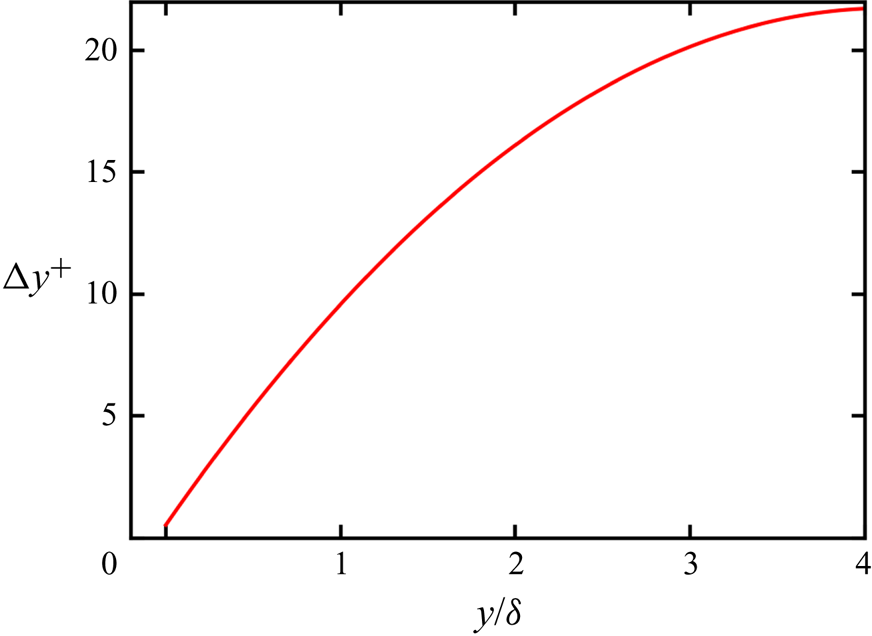
 ${\bar{\nu }_w}$ is the Reynolds-averaged kinematic viscosity of the fluid at the wall. The grids are clustered in the near-wall region in the wall-normal direction to better resolve the near-wall turbulence with nine grid points existing in the viscous sublayer, and gradually become coarser in the far field through a hyperbolic tangent function, as shown in figure 1. The minimum grid spacing is
 $\Delta y_{min}^ += 0.52$ at the wall. This mesh resolution is fine enough to capture small-scale turbulence in the near-wall region and the large-scale structures of the CTBL (Poggie, Bisek & Gosse Reference Poggie, Bisek and Gosse2015). The non-dimensional simulation time step is set as a constant at
 $\Delta t = 0.2$, thus giving a time step
 $\Delta {t^ + } = 0.033$ in wall units. With the present time step, the resultant Courant–Friedrichs–Lewy (CFL) number (defined as
 $\Delta t(\sqrt {{u^2} + {v^2} + {w^2}} + c)/h$, where h is the local grid size) in the whole computational field varies from 0.16 to 1.59.
Wall-normal grid distribution. Grid spacing  $\Delta {y^ + }$ is normalized by the viscous length scale at the downstream position of
 $R{e_\tau } = 500$.

At the wall, an isothermal no-slip Navier–Stokes characteristic boundary condition (NSCBC) is enforced (Poinsot and Lelef Reference Poinsot and Lelef1992). The wall temperature is set to be isothermal at a nominal adiabatic wall temperature as
 \begin{equation}{T_w} = \left( {1 + \frac{{r(\gamma - 1)}}{2}M{a^2}} \right){T_\infty }= 1.717,\end{equation}
where r is the recovery factor defined as  $r = P{r^{1/3}} = 0.896$ (Pirozzoli, Grasso & Gatski Reference Pirozzoli, Bernardini and Grasso2004). Compared with the truly adiabatic boundary condition (zero heat flux at the wall), it has been proved that this nominal adiabatic boundary condition shows no change to the mean-flow and fluctuation distributions, except for a little influence on the temperature fluctuations inside the viscous sublayer (see further discussions in Wenzel et al. (Reference Wenzel, Selent, Kloker and Rist2018)). Periodic boundary conditions are applied in the spanwise homogeneous direction. At the upper bound and streamwise outlet, non-reflecting NSCBCs (Poinsot and Lelef Reference Poinsot and Lelef1992) are imposed.
The inflow boundary conditions are prescribed with a fully developed compressible turbulent boundary layer field, which is extracted from a precursor DNS of a single-phase three-dimensional spatially developing CTBL. The initial field of this precursor simulation is set as a laminar compressible boundary layer at a Mach number of 2, the initial momentum thickness  ${\theta _{in}}$ of which is selected as the non-dimensional length scale. This gives a non-dimensional Reynolds number
 $Re = {\rho _0}{u_0}{\theta _{in}}/{\mu _0} = 180$. The precursor simulation has the same computational grids in the wall-normal and spanwise directions as in the main simulation, while having a longer streamwise computational domain of
 ${L_{x,pre}} = 8300$ with the same streamwise mesh resolution
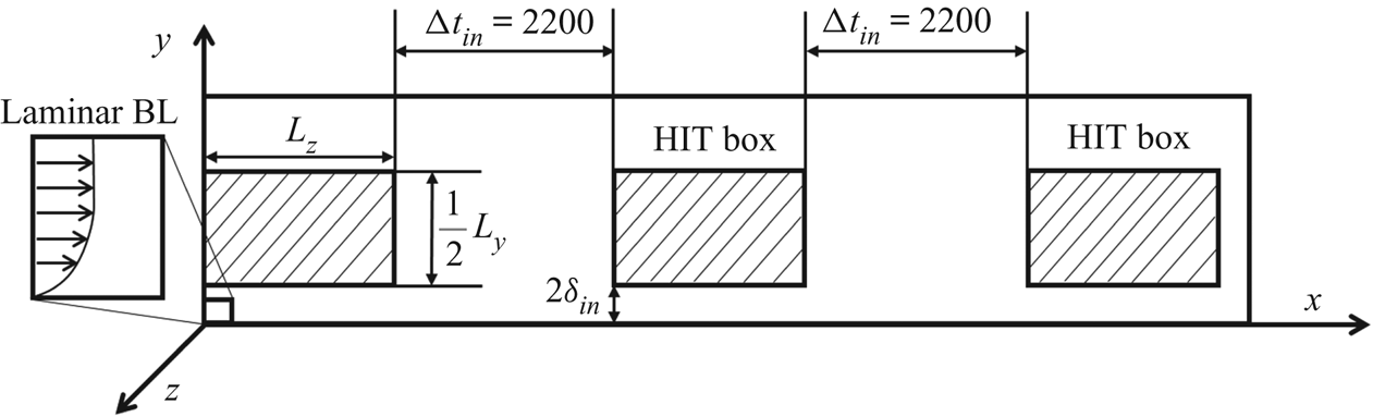
 $\Delta {x^ + } = 9.88$. To trigger the transition from a laminar state to a turbulent state of the boundary layer, an inflow boundary condition similar to that of Wu and Moin (Reference Wu, Bi, Hussain and She2009) and Li, Luo & Fan (Reference Li, Luo and Fan2016a) is specified. Every
 $\Delta {t_{in}} = 2200$, a box of homogeneous isotropic turbulence (HIT) is introduced to the velocity fields at the inlet plane, which will be convected downstream as shown in figure 2. This HIT is generated in a cubic box with an edge length of
 ${L_z}$ with a turbulent intensity of 3 %. To make the transition process more natural without destroying the laminar compressible boundary layer structure, the HIT box is placed at a distance of
 $2{\delta _{in}}$ (where
 ${\delta _{in}}$ is the laminar boundary layer thickness) from the wall, as illustrated in figure 2. To prevent unnecessary perturbations in the free stream in the far field, the upper half of the HIT box is removed, such that the HIT box can cover half the height of the computational domain.
Schematic of the inflow settings in the precursor simulation of a single-phase compressible transitional boundary layer.

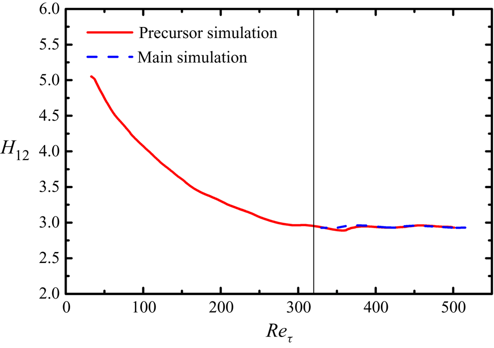
After transition, the flow field reaches a fully developed turbulent boundary layer state, with the influence of added HIT being negligible downstream. Then, a time series of the velocity, density and temperature data is extracted in the y–z plane with a friction Reynolds number  $R{e_\tau } = 321$, and used as the inflow conditions for the main simulation. The streamwise length of the precursor simulation is long enough to give a maximum friction Reynolds number
 $R{e_\tau } = 501$ at the outlet plane. The sample plane is relatively far away from the outlet plane to avoid possible boundary influence.
3.2. Particle characteristics
In this study, the particles are assumed to be Lagrangian rigid spheres with a constant diameter  ${d_p}$ and density
 ${\rho _p}= 1500$. After the TBL has developed for two convective periods,
 ${t_c} = {L_x}/{u_\infty } = 4450$, some particles are released at the inlet plane beneath the height
 $y = 160$, higher than the local boundary layer thickness at the exit plane. At every time step,
 ${N_{p,in}}(y)$ particles are released at the height y in the inlet plane to provide a uniform and constant particle mass fraction
 ${\varPhi _{m,in}}$ along the wall-normal direction. The particles are released randomly in a homogeneous spanwise direction. The inflow mass fraction of the particle phase
 ${\varPhi _{m,in}}$ is given as (Li et al. Reference Li, Fan, Luo and Cen2011)
 \begin{equation}{\varPhi _{m,in}} = \frac{{{\rho _p}{N_{p,in}}(y){\kern 1pt} {V_p}}}{{{{\bar{\rho }}_{in}}{\kern 1pt} {{\bar{u}}_{in}}(y){\kern 1pt} \Delta t{\kern 1pt} \Delta y{\kern 1pt} {L_z}}},\end{equation}
where  ${V_p}$ is the volume of a single particle,
 $\Delta t$ is the time-step interval,
 $\Delta y$ is the height of a computational cell at height y, and
 ${\bar{\rho }_{in}}$ and
 ${\bar{u}_{in}}$ are the Reynolds-averaged density and streamwise velocity at the inflow plane, respectively. The initial particle velocities are set as identical to the local fluid velocities. Because of the smaller fluid density and mass flux in the near-wall regions of a CTBL, the number of released particles at each time step in the near-wall regions is much smaller than that in the outer zones.
Two cases with different particle diameters are simulated to study particle motion and dispersion behaviours in the CTBL. Table 1 presents various parameters of the particles for the two cases, including particle Stokes number  $St$, viscous Stokes number
 $S{t^ + }$, particle density
 ${\rho _p}$, particle diameter
 ${d_p}$, ratio of particle diameter
 ${d_p}$ to minimum Kolmogorov length scale
 ${\eta _{min}}$, particle relaxation time
 ${\tau _p}$, inflow particle mass fraction
 ${\varPhi _{m,in}}$, particle volume fraction
 ${\varPhi _v}$ and particle number
 ${N_p}$ at the end of the simulation. The particle Stokes number
 $St = {\tau _p}/{\tau _f}$ is based on the particle relaxation time
 ${\tau _p} = Re{\rho _p}d_p^2/(18\mu )$ and characteristic flow time scale
 ${\tau _f} = \delta ^{\prime}/{u_\infty }$ (Ganapathisubramani et al. Reference Ganapathisubramani, Clemens and Dolling2006), where
 $\delta ^{\prime} = 144.4$ is the local boundary layer thickness in the downstream turbulent region of
 $R{e_\tau } = 500$. Using the wall viscous time scale
 ${t_v} = {\delta _v}/{u_\tau }$ as the characteristic flow time scale, the viscous Stokes numbers in cases A and B are
 $S{t^ + } = 2.36$ and
 $S{t^ + } = 24.33$, respectively. In both cases, the particle diameters are smaller than the Kolmogorov length scale
 ${\eta _w} = 0.415$ in the downstream turbulent region of
 $R{e_\tau } = 500$ at the wall, such that the Eulerian–Lagrangian point particle method can be employed. To maintain identical particle inflow numbers at the inlet for the two cases, different
 ${\varPhi _{m,in}}$ values are employed for the two cases. Considering the low ratio of the particle mass to the fluid mass and the particle-laden flow being dilute, the one-way coupling strategy is overall correct (Balachandar & Eaton Reference Balachandar and Eaton2010). However, the accumulation of particles at the wall would make it more reasonable to adopt the two-way coupling strategy, which may result in less-organized coherent structures (Li et al. Reference Li, Luo and Fan2016a), weaker wall accumulation and preferential accumulation of particles (Nasr, Ahmadi & McLaughlin Reference Nasr, Ahmadi and McLaughlin2009). Studies that include the backward influence of particles on fluid flow, i.e. two-way coupling, could be our future goal.
Particle parameters for the two cases.

Periodic boundary conditions are enforced for the particles in the homogeneous spanwise direction. Whenever a particle exits the outlet plane of the computational domain, it is removed from the simulation. Because of different degrees of preferential accumulation and the turbophoresis effect of particles caused by different degrees of particle inertia, the particle distribution and transportation are different for the two cases, causing different numbers of particles to exit the calculation domain at every time step. Therefore, the total number of particles  ${N_p}$ in the calculation domain at the end of the simulation is different for the two cases. The large height in the wall-normal direction of the calculation domain ensures that no particle can escape through the upper boundary. Particle–wall bouncing is assumed to be completely elastic.
3.3 A note on statistical averaging
In the present study, the particles are introduced in the calculation domain after evolution of the single-phase CTBL over two convective periods. The particle concentration and statistics reached a statistically quasi-steady state after two convective periods. Statistical data were then collected for another three convective periods. Statistical averaging was performed over time and over the homogeneous spanwise direction, as well as over a streamwise window of  $[{x_i} - {\delta _i}, {x_i} + {\delta _i}]$, where
 ${x_i}$ and
 ${\delta _i}$ correspond to a specific downstream position and the boundary layer thickness at this position.
For the averaging of fluid data in the Eulerian framework, the overbar (¯) and the prime (′) denote the Reynolds average and fluctuation. Statistical averages of Lagrangian particles were collected through averaging over all particles nearest to a local Eulerian grid in the statistical lifetime, thus providing the mapping of the statistical Lagrangian data to the Eulerian system.
4. Numerical validation
The present numerical schemes have been validated and adopted in previous studies on the interaction of detonation and inflow isotropic turbulence (Jin et al. Reference Jin, Luo, Dai and Fan2015), compressible jet flows (Luo et al. Reference Luo, Jin, Lu and Fan2013; Jin et al. Reference Jin, Luo, Dai and Fan2016), compressible HIT (Dai et al. Reference Di Marco, Camussi, Bernardini and Pirozzoli2017) and compressible mixing layers (Dai et al. Reference Dai, Jin, Luo and Fan2018, Reference Dai, Jin, Luo and Fan2019a,Reference Dai, Jin, Luo, Xiao and Fanb). In this section, the results of integral parameters and statistical characteristics of a single-phase CTBL are presented for validation.
4.1. Flow structure and integral parameters
In a CTBL, because of the variations of thermodynamic properties, the evolution of wall properties cannot be directly compared with that of properties in incompressible boundary layers. Thus, these integral parameters were compared with those under similar free-stream Mach number and friction Reynolds number  $R{e_\tau }$. The definitions of the integral parameters are
 \begin{gather}{\delta ^\ast } = \int_0^\delta {\left( {1 - \frac{{\bar{\rho }\bar{u}}}{{{\rho_\infty }{u_\infty }}}} \right)\textrm{d}y} ,\end{gather}
 \begin{gather}\theta = \int_0^\delta {\frac{{\bar{\rho }\bar{u}}}{{{\rho _\infty }{u_\infty }}}\left( {1 - \frac{{\bar{u}}}{{{u_\infty }}}} \right)\textrm{d}y} ,\end{gather}
 \begin{gather}{H_{12}} = \frac{{{\delta ^\ast }}}{\theta }\end{gather}
and
 \begin{equation}{C_f} = \frac{{{\tau _w}}}{{1/2{\rho _\infty }u_\infty ^2}},\end{equation}
where  ${\rho _\infty }$ and
 ${u_\infty }$ are the dimensionless density and streamwise velocity in the free stream;
 $\delta $ is the boundary layer thickness at which the Reynolds-averaged streamwise velocity is
 $0.99{u_\infty }$;
 ${\delta ^\ast }$ is displacement thickness;
 $\theta$ is momentum thickness;
 ${H_{12}}$ is shape factor; and
 ${C_f}$ is the skin friction coefficient. With these integral parameters, the corresponding integral Reynolds numbers are two momentum-thickness Reynolds numbers
 $R{e_\theta } = Re{\rho _\infty }{u_\infty }\theta /{\mu _\infty }$ and
 $R{e_{{\delta _2}}} = Re{\rho _\infty }{u_\infty }\theta /{\mu _w}$, friction Reynolds number
 $R{e_\tau } = Re{\rho _w}{u_\tau }\delta /{\mu _w}$ and friction Mach number
 ${M_\tau } = {u_\tau }/{(\gamma R{T_w})^{1/2}}$. The integral parameters are compared with the results of Pirozzoli & Bernardini (Reference Pirozzoli and Bernardini2011) and Shadloo, Hadjadj & Hussain (Reference Shadloo, Hadjadj and Hussain2015) at the same Mach number
 $Ma = 2$ and friction Reynolds number
 $R{e_\tau } = 500$ (table 2). Notably, a particularly good comparison can be achieved with the results of Pirozzoli & Bernardini (Reference Pirozzoli and Bernardini2011), which may be one of the most satisfactory statistical results for CTBL (Wenzel et al. Reference Wenzel, Selent, Kloker and Rist2018).
Boundary layer properties at specific positions.

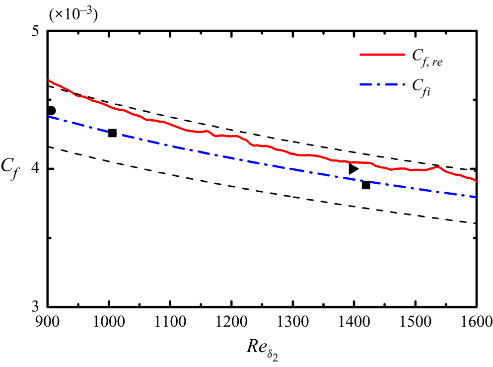
With the van Driest II transformation (van Driest Reference van Driest1956), the skin friction coefficients in a CTBL could be compared with incompressible counterparts through proper transformation. Here, the streamwise evolution of the rescaled skin friction coefficient  ${C_{f,re}}$ was compared with the incompressible results from Schlatter & Örlü (Reference Schlatter and Örlü2010) and compressible results from Pirozzoli & Bernardini (Reference Pirozzoli and Bernardini2011) and Pirozzoli, Bernardini & Grasso (Reference Pirozzoli, Grasso and Gatski2008), as well as a widely applied theoretical friction law (Smits, Matheson & Joubert Reference Smits, Matheson and Joubert1983) of
 ${C_{fi}} = 0.024Re_{{\delta _2}}^{ - 1/4}$ in figure 3. This rescaled friction coefficient
 ${C_{f,re}}$ in an adiabatic wall condition is expressed as
 ${C_{f,re}} = {F_c}{C_f}$, where
 ${F_c} = ({T_w}/{T_\infty } - 1)/{\arcsin ^2}\alpha $ and
 $\alpha = ({T_w}/{T_\infty } - 1)/\sqrt {{T_w}/{T_\infty }({T_w}/{T_\infty } - 1)}$. As shown in figure 3, the errors among
 ${C_{f,re}}$ and incompressible reference results and theoretical results are lower than 5 % in the whole region except in the immediate vicinity of the inlet, which may be caused by the treatment of the slices of inflow turbulence. In the present simulation, ghost cells outside the real computational domain are adopted to exert the boundary conditions. For the sake of saving storage, the inflow turbulent fields are only added to one layer of the ghost cells in the streamwise direction, with other layers being extrapolated. Besides the errors in the inlet regions, this treatment together with the underestimation of the van Driest II transformation (Pirozzoli & Bernardini Reference Pirozzoli and Bernardini2011; Wenzel et al. Reference Wenzel, Selent, Kloker and Rist2018) lead to the systematic error of the overhead of the rescaled friction coefficient. However, notably, this systematic error (<5 %) in the rear part of the present CTBL is thought to be small enough in some other DNS works (Duan, Beekman & Martín Reference Duan, Beekman and Martín2010, Reference Duan, Beekman and Martín2011; Wenzel et al. Reference Wenzel, Selent, Kloker and Rist2018). Therefore, we consider the comparison of skin friction coefficient to be satisfactory. To further investigate the role of the inflow region and the validity of the injected fully developed turbulence, the variation of the shape factors
 ${H_{12}}$ in the precursor simulation and the main simulation with friction Reynolds number is plotted in figure 4. It can be seen that the shape factor gradually decreases with the increase of the friction Reynolds number and becomes nearly constant after the friction Reynolds number reaches 321, the plane at which is extracted to serve as the inflow turbulence in the main simulation. As for the main simulation, the shape factor is almost the same constant as that in the precursor simulation, validating the equilibrium of the turbulent state (Pirozzoli & Bernardini Reference Pirozzoli and Bernardini2013).
Evolution of rescaled friction coefficients with the momentum thickness Reynolds number  $R{e_{{\delta _2}}}$. Squares denote incompressible DNS results by Schlatter & Örlü (Reference Schlatter and Örlü2010). Triangle denotes compressible DNS results by Pirozzoli & Bernardini (Reference Pirozzoli and Bernardini2011). Circle denotes compressible DNS results by Pirozzoli et al. (Reference Pirozzoli, Grasso and Gatski2008). Dashed lines indicate 5 % errors of
 ${C_{fi}}$.

Evolution of shape factors with the friction Reynolds number in the precursor and main simulations. The vertical line indicates the friction Reynolds number  $R{e_\tau } = 321$ where the inflow turbulent fields are extracted in the precursor simulation.

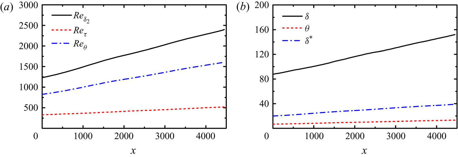
For the whole computational domain, the evolution of characteristic integral parameters in the streamwise direction is plotted in figure 5. All of these integral parameters develop nearly linearly in the streamwise direction and reach the maximum at the outlet. The characteristic Reynolds numbers have maxima of  $R{e_\tau } = 520$,
 $R{e_\theta } = 2400$ and
 $R{e_{{\delta _2}}} = 1612$. The displacement and momentum thickness at the outlet plane are
 ${\delta ^\ast } = 39$ and
 $\theta = 13.3$, respectively. The boundary layer thickness
 $\delta = 152$ is nearly a quarter of the calculation domain height, ensuring that the calculation domain is sufficiently high for turbulent boundary layer evolution (Poggie et al. Reference Poggie, Bisek and Gosse2015).
Evolutions of (a) characteristic boundary layer Reynolds numbers and (b) boundary layer integral parameters with the streamwise coordinate x.

4.2. Velocity statistics
The scaling of the mean velocity profile in a CTBL compared with that in an incompressible TBL remains an open question for high-Mach-number flows under complex wall heat transfer boundary conditions (Zhang et al. Reference Zhang, Bi, Hussain and She2014; Trettel & Larsson Reference Trettel and Larsson2016). Nevertheless, in the present study, at a moderate Mach number with an adiabatic wall, the van Driest transformation (van Driest Reference van Driest1951) for mean streamwise velocity and Morkovin's hypothesis (Morkovin Reference Morkovin1962) still hold true.
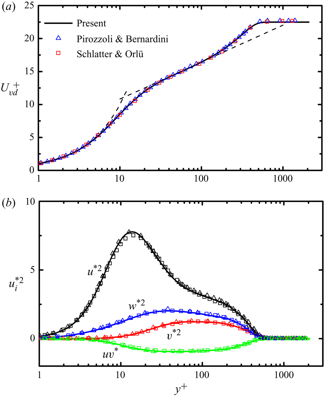
The van Driest transformation of velocity is defined as  ${u_{VD}} = \int {{{(\bar{\rho }/{{\bar{\rho }}_w})}^{1/2}}\,\textrm{d}\bar{u}}$. The mean streamwise velocity profile through transformation is expected to collapse to the incompressible velocity scaling law. In figure 6(a), the present results of the
 $u_{VD}^ +$ profile non-dimensionalized with the wall units were compared with the compressible results of Pirozzoli & Bernardini (Reference Pirozzoli and Bernardini2011) at a Mach number of 2 and the incompressible results of Schlatter & Örlü (Reference Schlatter and Örlü2010) in inner scaling at a similar friction Reynolds number; theoretical wall functions of
 ${u^ + } = {y^ + }$ and
 ${u^ + } = \ln ({y^ + })/0.41 + 5.2$ are also shown. At a similar friction Reynolds number, good agreement between compressible and incompressible data is achieved. The viscous sublayer law could hold until
 ${y^ + } \approx 5$, and the logarithmic law could hold from
 ${y^ + } \approx 30$ to
 ${y^ + } \approx 150$.
Comparison of (a) van Driest transformed mean streamwise velocity and (b) fluctuating velocity statistics in the present DNS at  $Ma = 2$ and
 $R{e_\tau } = 500$ (solid lines) with reference incompressible DNS data of Schlatter & Örlü (Reference Schlatter and Örlü2010) at
 $R{e_\tau } = 492$ (squares) and compressible DNS data of Pirozzoli & Bernardini (Reference Pirozzoli and Bernardini2011) at
 $Ma = 2$ and
 $R{e_\tau } = 497$ (triangles). Dashed lines in (a) represent the theoretical wall functions of
 ${u^ + } = {y^ + }$ and
 ${u^ + } = \ln ({y^ + })/0.41 + 5.2$.

Based on the Morkovin scaling, the distributions of density-scaled streamwise, spanwise and wall-normal velocity fluctuations, and Reynolds stress in inner scaling, are presented in figure 6(b), together with the compressible DNS results of Pirozzoli & Bernardini (Reference Pirozzoli and Bernardini2011) at a Mach number of 2 and the incompressible DNS results from Schlatter & Örlü (Reference Schlatter and Örlü2010) at a similar friction Reynolds number for comparison. This density-weighted normalized velocity fluctuation can be written as  $u_i^{{\ast} 2} = \bar{\rho }\,\overline {{{u^{\prime}}_i}{{u^{\prime}}_i}} /({\rho _w}u_\tau ^2)$. Again, good agreement is achieved between the compressible and incompressible results. These aforementioned validations ensure the capability of the present solver to capture the mean flow and fluctuation motions of a Mach 2 CTBL flow.
5. Results and discussion
5.1. Particle dispersion
5.1.1. Instantaneous visualization
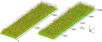
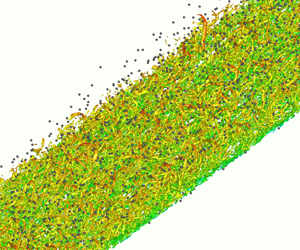
In figure 7, the three-dimensional instantaneous visualization of vortex structure and particle distribution in case B is displayed. The particles are represented by small grey dots. The vortex structures are identified by the Q-criterion (Hunt, Wray & Moin Reference Hunt, Wray and Moin1988) with an isosurface of  $Q = 0.0001$. Here Q is the second invariant of the instantaneous velocity gradient in compressible turbulence and is given as
 \begin{equation}Q = \frac{1}{2}\left( {{\theta^2} - {s_{ij}}{s_{ji}} + \frac{{{\omega_k}{\omega_k}}}{2}} \right) = \frac{1}{2}\left( {{{\left( {\frac{{\partial {u_i}}}{{\partial {x_i}}}} \right)}^2} - \frac{{\partial {u_i}}}{{\partial {x_j}}}\frac{{\partial {u_j}}}{{\partial {x_i}}}} \right),\end{equation}
where  $\theta = \partial {u_i}/\partial {x_i}$ is the divergence or dilatation,
 ${s_{ij}} = (\partial {u_i}/\partial {x_j} + \partial {u_j}/\partial {x_i})/2$ is the strain rate and
 ${\omega _k}$ is the vorticity in the kth direction. The vortical structures are coloured by the local streamwise velocity. Hairpin vortices are unsteady and irregular, indicating the fully developed state of a boundary layer flow, and particles are transported by these vortex structures within the boundary layer.
Instantaneous snapshot of three-dimensional vortical structures with Q criterion and particle configuration inside the computational domain in case B. The vortical structures are coloured by the local streamwise velocity (red and blue indicate high and low values respectively). Particles are indicated by small grey spheres (for better visualization, only parts of particles are shown).

5.1.2. Particle streaks
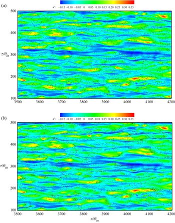
Figure 8 presents the instantaneous distributions of particles in a small region of the x–z plane at  ${y^ + } = 5$. The background contours are coloured with the local streamwise fluctuation velocity
 $u^{\prime}$. Particles are represented by grey dots. In case A, the particles distribute very uniformly in the x–z plane. For this small Stokes number, the particles could be seen to be efficiently tracing with small-scale fluctuations so that no apparent preferential concentration occurs. By contrast, in case B, the particle streaks are clearly formed in the low-speed regions, which are associated with negative local streamwise fluctuation velocity. This result is similar to the DNS results reported by Mortimer, Njobuenwu & Fairweather (Reference Mortimer, Njobuenwu and Fairweather2019) for turbulent channel flows, in which the authors concluded that particles with a viscous Stokes number
 $S{t^ + } = 25$ have the strongest tendency to form particle streaks compared with higher or lower relaxation time. Thus, preferential clustering near the wall is much stronger in case B than in case A. This is further discussed quantitatively later on. In both cases, the low-speed regions are numerous and elongated, whereas the high-speed regions are smaller but more intense. This characteristic is identical to that in incompressible TBLs (Robinson, Kline & Spalart Reference Robinson, Kline and Spalart1989).
Particle distribution in a small region with  ${y^ + } = 5$ in (a) case A and (b) case B. Colours represent the values of the streamwise fluctuation velocity
 $u^{\prime}$.

5.1.3. Self-similar feature of particle number density
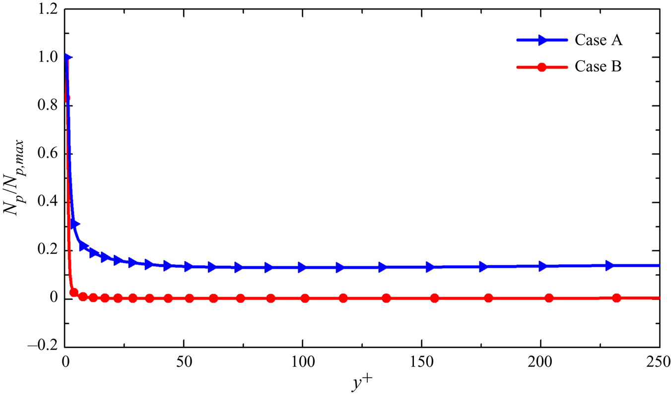
The particles are introduced with a constant mass fraction at the inlet plane along the wall-normal direction; in other words, in the near-wall low-speed region, fewer particles are released but many particles are clustered. From figure 8, it can be seen that the particle concentration is much higher in case B than in case A. This trend can also be noted in the distribution of the normalized particle number densities at a friction Reynolds number  $R{e_\tau } = 500$ in the wall-normal direction in figure 9, where the particle number densities are normalized by the maximum number density
 ${N_{p,max}}$ at the wall. The high particle concentration in the near-wall regions provides a much lower normalized particle number density in case B than in case A.
Wall-normal profiles of the particle number density  ${N_p}$ normalized by the maximum particle number density
 ${N_{p,max}}$ at
 $R{e_\tau } = 500$.

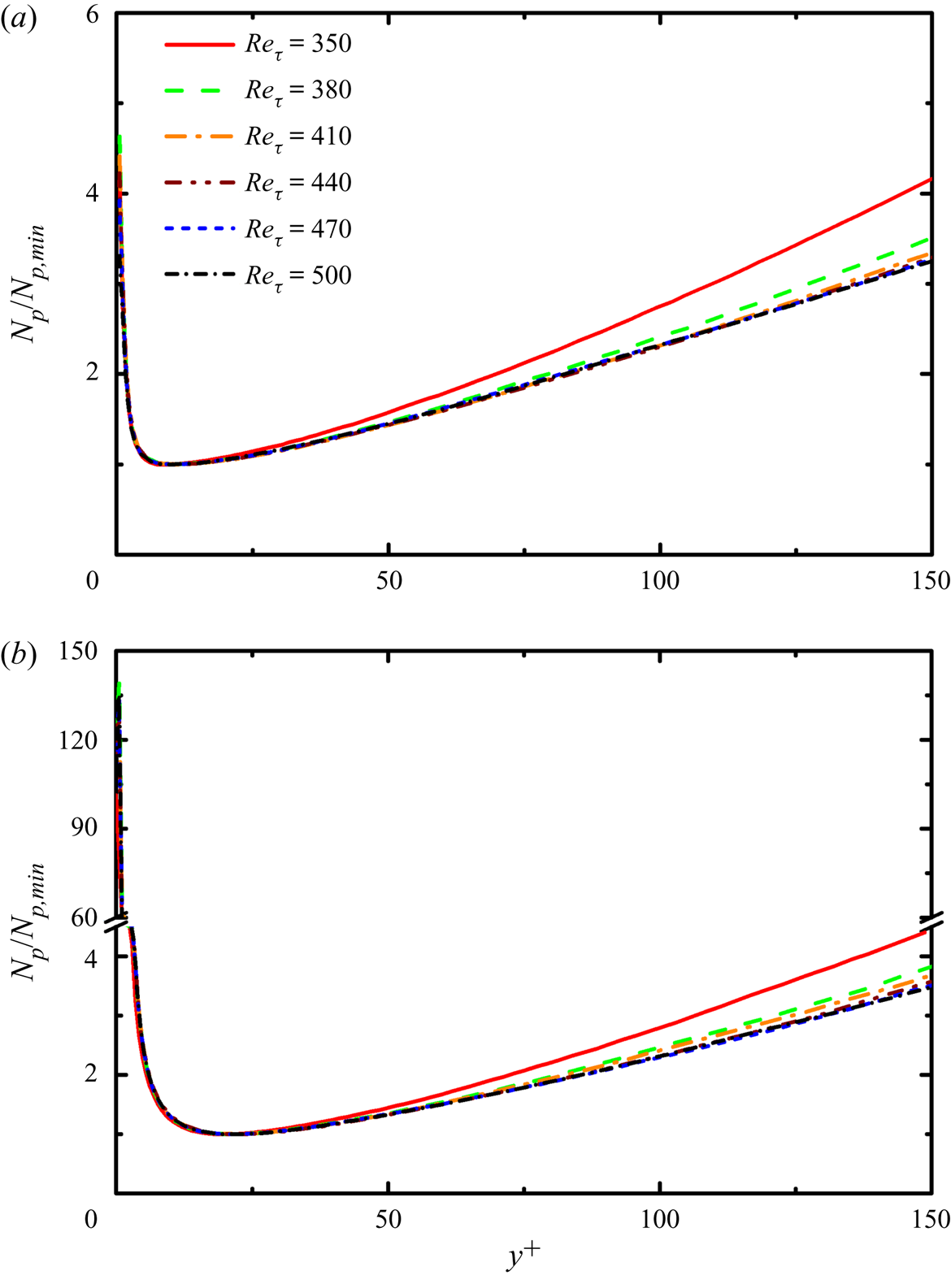
To provide additional details of the particle dispersion within the boundary layer, we focus on another normalized particle number density profile. Similar to the multiphase incompressible TBL results of Sardina et al. (Reference Sardina, Schlatter, Picano, Casciola, Brandt and Henningson2012b), there exists a minimum particle number density  ${N_{p,min}}$ in the viscous sublayer in the present CTBL. In cases A and B, the minimum
 ${N_{p,min}}$ occurs at
 ${y^ + } \approx 10$ and
 ${y^ + } \approx 20$, respectively. After normalization by
 ${N_{p,min}}$, the wall-normal profile of
 ${N_p}/{N_{p,min}}$ attains a self-similar distribution in wall units after some streamwise development in both cases, as shown in figure 10. The near-wall particle number density is much higher in case B than in case A, indicating strong wall accumulation caused by turbophoresis due to the greater particle inertia. As mentioned, in case B we have
 $St_{}^ += 24.33$; this viscous Stokes number is in the range for inducing maximum wall accumulation reported by Marchioli & Soldati (Reference Marchioli and Soldati2002) for incompressible channel flow and by Sardina et al. (Reference Li and Bai2012a) for incompressible boundary layer flow, where the maximum wall accumulation occurred when
 $St_{}^ +\approx 29$ and
 $10 \lt St + \lt 50$, respectively.
Wall-normal profiles of the particle number density  ${N_p}$ normalized by the minimum particle number density
 ${N_{p,min}}$ in (a) case A and (b) case B at different friction Reynolds numbers.

Although one-way coupling is adopted in this study and the particles are released with the same number densities at the inflow plane for different diameters (Stokes number), the characteristics of near-wall accumulation and preferential clustering are much different in the two cases. These two processes are much more pronounced in case B, displaying a strong influence of particle inertia on particle dispersion. Most studies on wall-bounded turbulent flows laden with particles have been performed in channel flows. Because of the periodicity of streamwise direction in channel flow, knowledge of the evolution of the particle concentration in the streamwise direction is limited. Notably, a self-similar feature of the particle number density profile in a CTBL is observed, as presented in figure 10.
Another main difference between multiphase channel flow and boundary layer flow is that, in channel flows, the particle concentration can reach a quasi-steady state after the evolution of several convective periods, whereas in boundary layer flows, the quasi-steady state of the particle concentration can barely be achieved because many particles are entrained in the viscous sublayer and move very slowly in the streamwise direction. In this study, even though the flow had developed for five convective periods, most particles in the viscous sublayer could not travel the length of the calculation domain in the streamwise direction because of the long residual time and low streamwise velocity. This also indicates that, in the downstream regions, particles trapped in the viscous sublayer are not transported in the streamwise direction from upstream but entrained by vortices to reach the wall regions. Near-wall vortex structures dominate particle motions to form the maximum concentration at the wall and local minimum concentration in the near-wall regions. Furthermore, normalized by the minimum number density  ${N_{p,min}}$, the self-similar feature of the particle number density at different streamwise locations is sustained in the wall units. Considering that the self-similar feature of the particle number density demonstrates much stronger wall accumulation in case B than in case A, and that the only difference between cases A and B is the particle diameter (inertia), the self-similar characteristics might only be affected by particle inertia.
5.2. Particle statistics
5.2.1. Particle mean and slip velocity
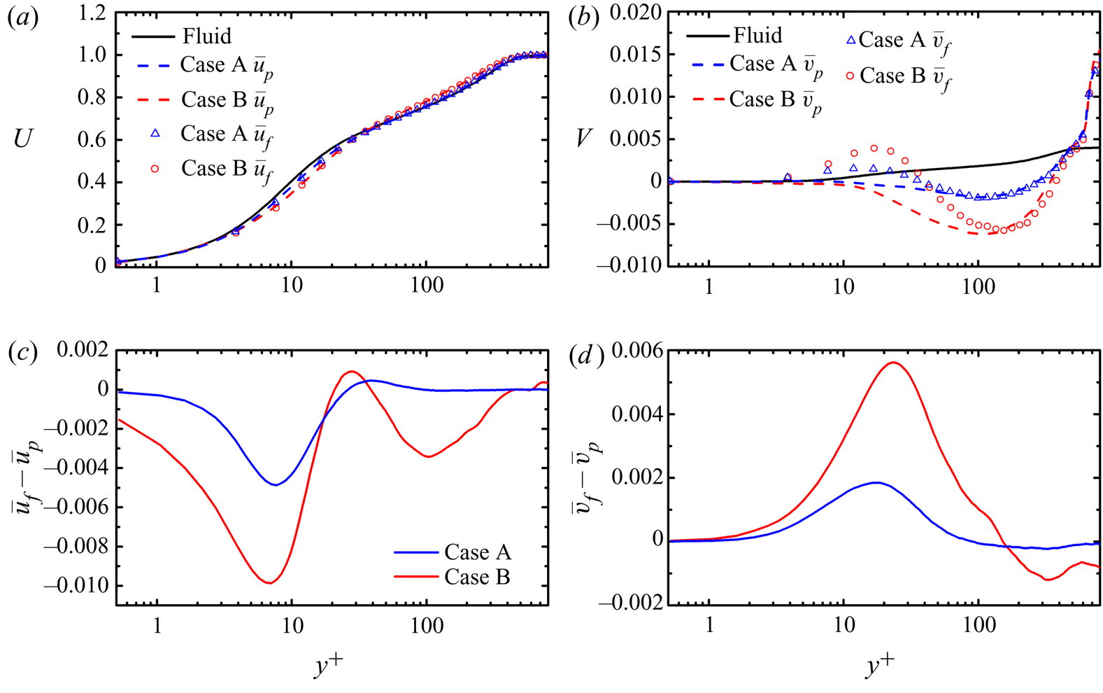
To investigate the differences between particle motion and fluid motion, we plot the wall-normal profile of mean particle streamwise velocity  ${\bar{u}_p}$ and streamwise fluid velocity at the particle positions
 ${\bar{u}_f}$ in cases A and B along with the mean streamwise fluid velocity
 $\bar{u}$ in figure 11. These data are extracted at the downstream region of the friction Reynolds number
 $R{e_\tau } = 500$.
Mean particle velocity (dashed lines), the fluid velocity seen by particles (symbols), and the mean fluid velocity (black solid line) in (a) streamwise and (b) wall-normal directions. Mean slip velocity in (c) the streamwise direction  $({\bar{u}_f} - {\bar{u}_p})$ and (d) in the wall-normal direction
 $({\bar{v}_f} - {\bar{v}_p})$.

In the near-wall regions, the particle streamwise velocity  ${\bar{u}_p}$ is lower than the fluid streamwise velocity. This is the result of particle preferential accumulation in the near-wall streaks, which corresponds to low streamwise velocity. However, after reaching a critical height, the particle streamwise velocity
 ${\bar{u}_p}$ exceeds the streamwise fluid velocity. This trend is stronger for large particles with
 $St = 1$ in case B. The critical height is at
 ${y^ + } \approx 45$ in the present CTBL, in contrast to that of
 ${y^ + } \approx 18$ in the results reported by Zhao, Marchioli & Andersson (Reference Zhao, Marchioli and Andersson2012) on incompressible two-phase channel flow at a friction Reynolds number
 $R{e_\tau } = 150$.
Consider the streamwise particle slip velocity, namely the difference between the fluid streamwise velocity seen by particles and particle streamwise velocity  ${\bar{u}_f} - {\bar{u}_p}$: it is negative in the near-wall regions, positive in the lower parts of the logarithmic layer, and negative in the outer region, as shown in figure 11(c). A greater deviation of
 ${\bar{u}_f} - {\bar{u}_p}$ to zero in case B means that the preferential accumulation in case B is more significant. A similar tendency of the streamwise velocity difference was reported by Sardina et al. (Reference Sardina, Schlatter, Picano, Casciola, Brandt and Henningson2012b) for incompressible TBL and by Zhao et al. (Reference Zhao, Marchioli and Andersson2012) for incompressible turbulent channel flow. However, this difference is too small within the boundary layer region to cause a distinct difference between
 ${\bar{u}_p}$ and
 ${\bar{u}_f}$. This is in contrast to the results of Zhao et al. (Reference Zhao, Marchioli and Andersson2012), who reported that, at viscous Stokes numbers of
 $S{t^ + } = 30$ and
 $S{t^ + } = 5$ similar to those used in the present study, the maximum of streamwise slip velocity could reach 0.2 and 0.1, respectively. This deviation is possibly because of the suppression of turbulence due to the decrease of the fluid mean density at the wall (Duan et al. Reference Duan, Beekman and Martín2011), which attenuates the near-wall small-scale turbulence and the particle slip velocity.
Regarding the wall-normal component, as shown in figure 11(b), although the mean fluid wall-normal velocity is positive because of the mean flow gradient, the particle velocity is negative beneath the height  ${y^ + } \approx 300$ in both cases, with its maximum occurring at
 ${y^ + } \approx 100$. The maximum value indicates the strongest tendency of the fluid to sweep particles towards the wall. As the distance between particles and the wall decreases, the wall-oriented velocity of particles decreases as a result of the low fluid velocity. The wall-oriented velocity increases with the increase in particle inertia in the near-wall regions. Similar trends were obtained by Picciotto et al. (Reference Picciotto, Marchioli, Reeks and Soldati2005a) for incompressible channel flow. However, in the outer layer, the wall-normal velocity is almost identical for both particle types and is much larger than that for the fluid. This phenomenon may be due to the lack of particles in the higher region above the wall. The wall-normal velocity of particles equals the fluid velocity at
 ${y^ + } \approx 500$ or equivalently at
 $y \approx 144$, and this is very close to the upper bound of
 $y = 160$ at the inlet plane to inject particles. Thus, particles mainly have two pathways for reaching this height: one is being injected at the inlet and barely being affected by the boundary layer turbulence, and the other is being lifted from the inner region and gradually decelerated in the wall-normal direction. Although the particle number is relatively low, particles at this height cannot be swept towards the wall. Thus, only the positive wall-normal velocity seen by particles can be recorded.
In the viscous sublayer and buffer layer, the fluid velocity seen at the particle positions is greater than the particle velocity, which indicates that the particles are under an uplifted drag force. In the two types of particles considered here, the fluid velocity seen at the particle positions in case B is much larger than that in case A, thus leading to a larger wall-normal slip velocity  ${\bar{v}_f} - {\bar{v}_p}$ in case B, as shown in figure 11(d). The profiles of
 ${\bar{v}_f} - {\bar{v}_p}$ show a tendency similar to that reported by Zhao et al. (Reference Zhao, Marchioli and Andersson2012). However, analogous to the streamwise slip velocity, the wall-normal slip velocity here is much smaller than that in incompressible channel flow by Zhao et al. (Reference Zhao, Marchioli and Andersson2012). The difference between the fluid velocity seen in particle position
 ${\bar{v}_f}$ and the mean velocity
 $\bar{v}$ may be attributable to the preferential clustering of particles in ejection regions, corresponding to positive wall-normal fluid velocity regions. When
 ${\bar{v}_f}$ is larger than
 $\bar{v}$, more particles are located in these ejection regions. Because in our simulations only one-way coupling was considered such that the turbulent fields in both cases are the same, the difference in wall-normal slip velocity in cases A and B is also a quantitative indicator for stronger preferential clustering in case B.
5.3. Mechanism analysis for particle motion and accumulation
In the previous sections, we report the investigation of particle preferential accumulation and particle mean statistics in CTBLs. In this section, we provide further insight into the physical mechanisms causing the particle's statistical characteristics and preferential accumulation.
5.3.1. Influence of vortex on particle statistics
In the study of incompressible wall-bounded flows, the near-wall coherent dynamic structures are potentially responsible for the particle motion, accumulation and segregation (Kaftori et al. Reference Kaftori, Hetsroni and Banerjee1995a). A series of near-wall turbulent structures, including sweep and ejection processes, quasi-streamwise vortex and streak structures, and particle inertia, simultaneously govern the near-wall accumulation and preferential clustering of particles. Abundant research has focused on the study of these processes. McLaughlin (Reference McLaughlin1989) simulated particle deposition in vertical incompressible channel flows and found that particles accumulated in the viscous sublayer as a result of sweep events. The author indicated that, although vortex motion led particles to be pushed away from the wall, this wall-normal velocity was much slower than that given by strong sweep events, resulting in a very long residence time in the viscous sublayer for particles. In their experimental studies, Kaftori et al. (Reference Kaftori, Hetsroni and Banerjee1995a,Reference Kaftori, Hetsroni and Banerjeeb) concluded that, in the near-wall regions, particles are controlled by coherent vortex structures, thus forming particle streaks in the viscous sublayer.
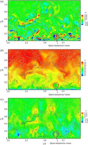
In a CTBL, the dynamics of turbulent structures is similar to that in an incompressible TBL (Pirozzoli et al. Reference Pirozzoli, Grasso and Gatski2008). The boundary layer turbulence is characterized by the self-sustained sweep and ejection events in near-wall regions and very-large-scale motion in the outer regions. Similarly, the motion of particles in CTBLs is significantly influenced by the evolution of quasi-streamwise vortices and sweep and ejection events. Figure 12 shows the instantaneous contours of (a) streamwise vorticity  ${\omega _x}$, (b) streamwise velocity, and (c) wall-normal velocity in the y–z plane at the downstream position with the friction Reynolds number
 $R{e_\tau } = 500$, together with the superimposed particles in case A. The particles are represented by gold dots, and the particle instantaneous velocities in the transverse direction are represented by arrowed vectors. As shown in figure 12(a), the near-wall regions contain a pair of counter-rotating quasi-streamwise vortices, highlighted by a red circle and a pair of counter-rotating arrows indicating the rotation of the quasi-streamwise vortices. Particles tend to accumulate at the edge of quasi-streamwise vortices and move circularly with the upwash and downwash of the fluid while leaving few particles in the core region of the vortex. The middle of these two vortices in the y–z plane contains a local minimum of streamwise velocity and maximum of wall-normal velocity, as shown in figure 12(b) and (c), which correspond to the ejection events of
 $u^{\prime} \lt 0$ and
 $v^{\prime} \gt 0$. At the bottom of these vortices, an extremely low streamwise velocity is observed (the blue area beneath the red circle in figure 12b), indicating the presence of a near-wall low-speed region beneath the quasi-streamwise vortices consistent with the findings by Ringuette, Wu & Martín (Reference Ringuette, Wu and Martín2008). In the sweep regions, particles are driven towards the wall with
 $u^{\prime} \gt 0$ and
 $v^{\prime} \lt 0$; in the ejection regions, particles move away from the wall with
 $u^{\prime} \lt 0$ and
 $v^{\prime} \gt 0$.
Instantaneous contours of (a) streamwise vorticity, (b) streamwise velocity, (c) wall-normal velocity and vectors of the particle velocity at  $R{e_\tau } = 500$ in case A.

To better understand the relationship between the particle dispersion and the coherent wall structures in the CTBL, a conditional sampling procedure is performed for the particles around the streamwise position where the friction Reynolds number  $R{e_\tau } = 500$. The statistics are averaged in the streamwise and spanwise directions over the same time period as introduced in the statistical averaging of fluid data in § 3.3. After applying conditional sampling for particles in cases A and B, the ratios of particles residing in different quadrants Q1 (
 $u^{\prime} \gt 0$ and
 $v^{\prime} \gt 0$), Q2 (ejection,
 $u^{\prime} \lt 0$ and
 $v^{\prime} \gt 0$), Q3 (
 $u^{\prime} \lt 0$ and
 $v^{\prime} \lt 0$) and Q4 (sweep,
 $u^{\prime} \gt 0$ and
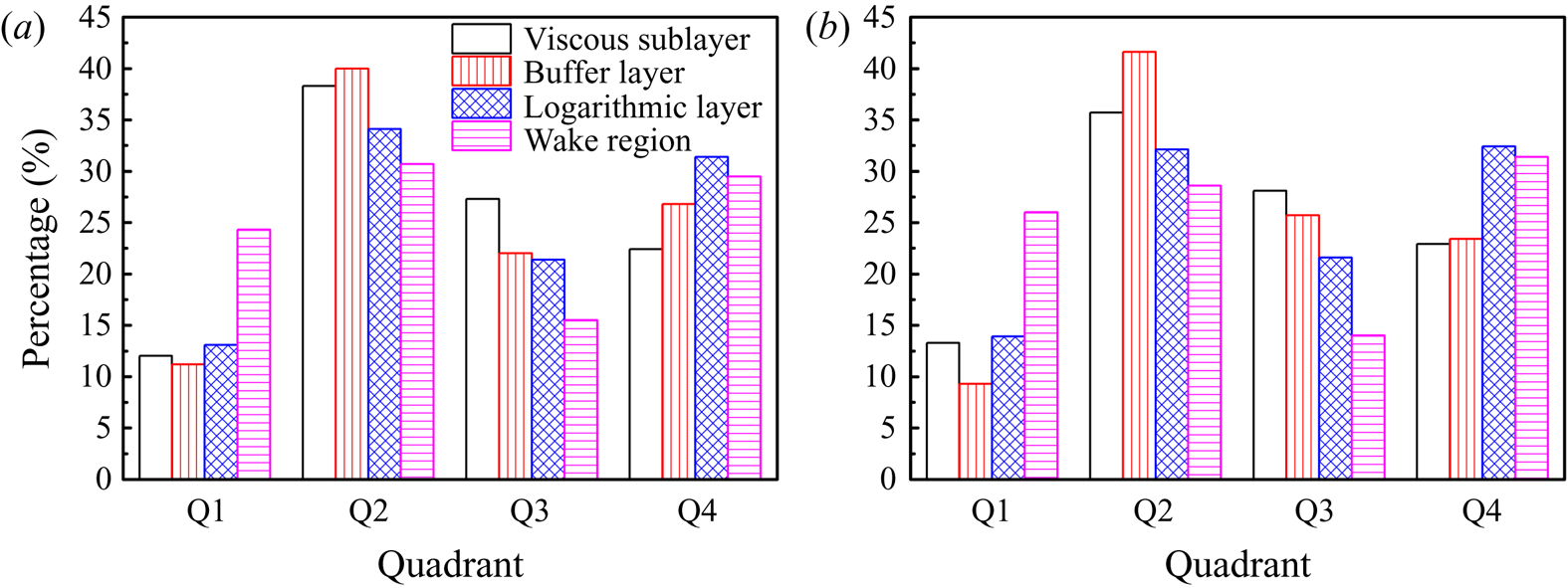
 $v^{\prime} \lt 0$) in different regions are illustrated in figure 13. We note that in cases A and B, 65.3 % and 62.3 % of particles reside in the regions of
 $u^{\prime}v^{\prime} \lt 0$, respectively, i.e. coherent sweep and ejection regions, beneath the edge of the logarithmic layer at
 ${y^ + } = 150$, in which 35.7 % and 34.9 % are in Q2 (ejection), respectively, and 29.6 % and 27.4 % are in Q4 (sweep), respectively. Notably, particles are mainly accumulated in Q2 (sweep) and Q4 (ejection) in all regions in both cases because of the influence of the quasi-streamwise vortex and particle inertia. In the viscous sublayer and buffer layer, the particle accumulation is significant in ejection regions (39.4 % and 37.3 % in cases A and B). The differences between particle numbers in the sweep and ejection regions originate at a low velocity in the viscous sublayer, causing difficulty for the particles brought into the viscous sublayer by sweeps in accelerating and leaving the near-wall region.
This can also be illustrated quantitatively by the wall-normal velocity of the particles conditionally averaged in the sweep and ejection regions. Although the ratios of the particles in the sweep and ejection regions are similar for different particle inertia (diameter), the conditional averaging shows significant differences in statistics. In cases A and B, the wall-normal velocities of the particles averaged in the sweep regions become
 ${v_{p,sw}} ={-} 0.01531$ and
 ${v_{p,sw}} ={-} 0.00537$, respectively, and those in the ejection regions become
 ${v_{p,ej}} = 0.01255$ and
 ${v_{p,ej}} = 0.00217$, respectively. Because of higher particle inertia of the large particles, which prevents their motion following the local fluid, the velocities of particles are lower in case B than in case A. The wall region is dominated by ejection events; therefore, particles typically accumulate in ejection regions, leading to a higher wall-normal velocity of fluid seen by particles, as shown in figure 11(b).
Ratios of particle residing in different quadrant in (a) case A and (b) case B in different regions.

In the wake regions and near the edge of the boundary layer, as can be seen in figure 12(a), particles are drifted by large-scale quasi-streamwise vortex structures and accumulate in the low-vorticity region. In the wake region, most particles remain residing in the coherent sweep and ejection regions in cases A and B, with 29.5 % and 31.4 % of particles in sweep regions, respectively, and 30.7 % and 28.6 % in ejection regions, respectively. One significant difference of the particle dispersion in the wake region from that in the near-wall regions is the accumulation of particles in Q1 regions in cases A and B, as shown in figure 13. There are 24.3 % and 26.0 % of particles residing in Q1 regions for cases A and B, respectively, which are nearly twice those in the viscous sublayer, buffer layer and logarithmic layer. The accumulation of particles in Q1 regions may contribute to the greater Reynolds-averaged streamwise velocity of the particles compared to that of the fluid.
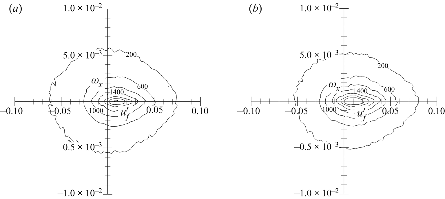
To illustrate this phenomenon and the underlying mechanisms, we plot the two-dimensional joint probability density function (p.d.f.) of the streamwise fluid fluctuation velocity  ${u^{\prime}_f}$ and streamwise vorticity
 ${\omega _x}$ seen at the particle positions in the wake regions in figure 14. In both cases, particles tend to accumulate in the low-streamwise-vorticity regions because of the centrifugal force driven by the quasi-streamwise vortex. The preferential accumulation in this dimension is stronger in case B because of a stronger inertial effect. Preferential accumulation in the regions of
 ${u^{\prime}_f} \gt 0$ indicates that particles are clustered in the sweep regions with
 $u^{\prime} \gt 0$ and
 $v^{\prime} \lt 0$. This results from the prevalence of sweep events in the outer regions (Jiménez Reference Jiménez2018). The two aforementioned mechanisms together lead to an increased average streamwise velocity for particles compared with that for the fluid, particularly in case B. Although particles are clustered in the sweep regions, the average wall-normal velocity of the particles is positive at this height away from the wall. This is due to the presence of few particles at this height, and particles reach this region mainly as a result of the residual effect of ejections, as previously demonstrated. Further beyond the local boundary layer thickness, the particles move at the same streamwise velocity as the fluid with almost zero transverse velocity.
Two-dimensional PDF of the streamwise fluid fluctuation velocity  ${u^{\prime}_f}$ and streamwise vorticity
 ${\omega _x}$ seen at the particle positions in the wake regions in (a) case A and (b) case B.

5.3.2. Mechanism analysis of preferential accumulation
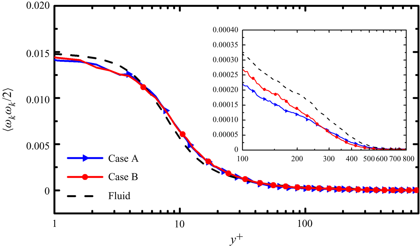
In general, the particles are significantly influenced by the centrifugal effect of the vortex structure and accumulate in low-vorticity regions. In compressible turbulence, these regions correspond to the compression of fluid outside the vortex core. By contrast, the high-vorticity core region corresponds to the expansion of fluid at a low density. Thus, particles have a tendency to cluster in high-density regions (Dai et al. Reference Di Marco, Camussi, Bernardini and Pirozzoli2017). However, in near-wall regions, particles are characterized by low-speed streaks (Li et al. Reference Li, Wei, Luo and Fan2016b) and are likely to accumulate in low-density regions. Thus, the two mechanisms simultaneously govern particle motion in CTBLs. Characterization of the particle dispersion by the classical low-vorticity accumulation theory is inaccurate because of the presence of the wall. In figure 15 we plot the profile of the enstrophy  $\langle {\omega _k}{\omega _k}/2\rangle $ conditionally averaged at particle positions and at the fluid points in the wall-normal direction, where the bracket ‘
 $\langle\,\rangle $’ means conditional averages. In the buffer layer, the conditionally averaged enstrophy at particle positions in cases A and B is larger than that of the fluid; thus, particles accumulate more selectively in higher-vorticity regions. In the viscous sublayer, logarithmic layer and wake regions, the fluid enstrophy seen at the particle positions is smaller than that of the fluid, which is in agreement with the classical theory.
Comparison of enstrophy  $\langle {\omega _k}{\omega _k}/2\rangle $ conditionally averaged at particle positions with that at the fluid points.

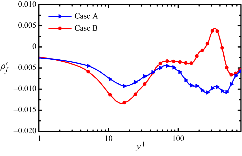
As mentioned, the preferential accumulation of particles in low-vorticity and high-density regions is due to the centrifugal effect of the vortex. However, in near-wall regions, the wall effect and the dominance of ejection events lead particles to accumulate in low-density regions, which may counteract the mechanism of preferential accumulation caused by the centrifugal effect. To better illustrate this phenomenon, we plot the wall-normal profile of the fluctuation density of fluid  $\langle {\rho ^{\prime}_f}\rangle = {(\rho - \bar{\rho })_p}$ conditionally averaged at the particle positions in figure 16 collected with the same conditional sampling technique as introduced in § 5.3.1. Notably, if the fluctuation density of the fluid is Reynolds-averaged at fluid points while not at the particle positions, it should be zero because the Reynolds-averaged value of a fluctuating quantity is zero. Therefore, the value of
 $\langle {\rho ^{\prime}_f}\rangle$ conditionally averaged at the particle positions can indicate the variation of particle accumulation with fluid density.
Wall-normal profiles of the fluid fluctuation density seen at the particle positions.

As can be seen from figure 16, in the viscous sublayer and buffer layer, both particles accumulate in the regions of low fluid density. The maximum negative fluid density fluctuation occurs at  ${y^ + } \approx 15$ in both cases. By applying conditional sampling at this slice of
 ${y^ + } \approx 15$, the conditionally averaged enstrophy at the fluid points with negative density fluctuation (0.0033) is close to enstrophy at particle positions (0.0035 in case A and 0.0036 in case B) and higher than that averaged across all of the fluid points (0.0029), demonstrating the preferential accumulation of particles in low-density and high-vorticity near-wall regions. With increasing distance away from the wall,
 $\langle {\rho ^{\prime}_f}\rangle$ gradually increases in case B and reaches a positive maximum, whereas in case A,
 $\langle {\rho ^{\prime}_f}\rangle$ remains negative. This evolution of the
 ${\rho ^{\prime}_f}$ profile in the wall direction and the different behaviours of particle accumulation according to density have never before been reported.
To reveal the mechanism underlying the selective accumulation of particles on the basis of fluid fluctuation density, we consider the governing equation of particle velocity (Picano et al. Reference Picano, Battista, Troiani and Casciola2011):
 \begin{equation}{v_{p,i}} = {u_{p,i}} - \frac{{{\tau _p}}}{{{f_1}}}\frac{{\textrm{d}{u_{p,i}}}}{{\textrm{d}t}} + O(\tau _p^2).\end{equation}
For small particles in case A, the particle relaxation time scale  ${\tau _p}$ is smaller than the Kolmogorov time scale
 ${\tau _\eta }$, such that the second-order correction
 $O(\tau _p^2)$ can be neglected, and the evolution of particle velocity can be given as
 \begin{equation}{v_{p,i}} = {u_{p,i}} - \frac{{{\tau _p}}}{{{f_1}}}\frac{{\textrm{d}{u_{p,i}}}}{{\textrm{d}t}}.\end{equation}
Taking the divergence of this equation, we can obtain an equation representing the dilatation of particles (Zhang et al. Reference Zhang, Bi, Hussain, Li and She2016; Dai et al. Reference Di Marco, Camussi, Bernardini and Pirozzoli2017):
 \begin{equation}\boldsymbol{\nabla} \boldsymbol{\cdot} {\boldsymbol{v}_p} - \boldsymbol{\nabla} \boldsymbol{\cdot} {\boldsymbol{u}_p} ={-} \frac{{{\tau _p}}}{{{f_1}}}{\left[ {\frac{1}{{Re}}\frac{\partial }{{\partial {x_i}}}\left( {\frac{1}{\rho }\frac{{\partial {\sigma_{ij}}}}{{\partial {x_j}}}} \right) - \frac{1}{{\gamma {M^2}}}\frac{\partial }{{\partial {x_i}}}\left( {\frac{1}{\rho }\frac{{\partial p}}{{\partial {x_i}}}} \right)} \right]_p} ={-} \frac{{{\tau _p}}}{{{f_1}}}{\Theta _p},\end{equation}
where the subscript p represents the fluid properties calculated at particle positions. In the regions of particle clustering, the dilatation of particles should be smaller than that of the local fluid and the value of  $\boldsymbol{\nabla} \boldsymbol{\cdot} {\boldsymbol{v}_p} - \boldsymbol{\nabla} \boldsymbol{\cdot} {\boldsymbol{u}_p}$ should be negative (Dai et al. Reference Di Marco, Camussi, Bernardini and Pirozzoli2017).
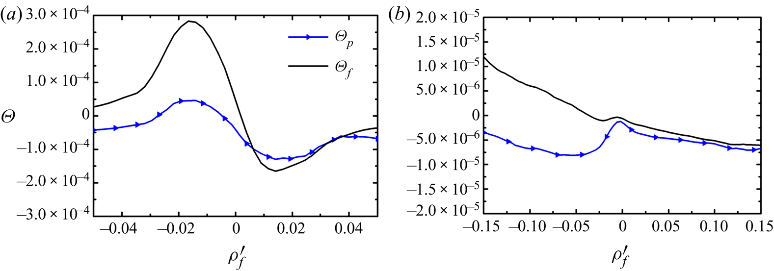
Considering the very-near-wall regions (viscous sublayer and buffer layer) and wake regions with distinct fluid density fluctuations, we plot the conditionally sampled  $\varTheta$ at the particle positions
 $({\varTheta _p})$ and at the fluid points
 $({\varTheta _f})$ in case A in figure 17. Because of the large particle inertia in case B and the fact that the second-order correction
 $O(\tau _p^2)$ cannot be ignored, the aforementioned analysis cannot be applied to case B; the corresponding figure in case B has hence not been included.
Comparisons of  $\varTheta$ conditionally sampled at the particle positions
 $({\varTheta _p})$ and at fluid points
 $({\varTheta _f})$ in (a) very-near-wall regions and (b) wake regions in case A.

As shown in figure 17(a), when  ${\rho ^{\prime}_f} \gt 0$, i.e. in the regions of high density or positive fluid density fluctuation,
 ${\varTheta _p}$ is nearly identical to
 ${\varTheta _f}$ in the very-near-wall regions. In other words, in the regions with positive fluid density fluctuation, the accumulation of particles on the basis of positive density fluctuation is weak. However,
 ${\varTheta _p}$ is much smaller than
 ${\varTheta _f}$ in the regions of negative fluid density fluctuation
 ${\rho ^{\prime}_f} \lt 0$. A negative (although
 ${\varTheta _p} \lt 0$ is not strictly guaranteed) and smaller value of
 ${\varTheta _p}$ than
 ${\varTheta _f}$ quantitatively demonstrates that particles are accumulated in the regions of negative fluid density fluctuation as analysed in (5.4). Therefore, the fluid density conditionally averaged at the particle positions is lower than that at fluid points, leading to a negative fluid density fluctuation seen at the particle positions in the very-near-wall regions as shown in figure 16. Qualitatively, in the very-near-wall regions in both cases A and B, negative
 ${\rho ^{\prime}_f}$ is caused by the correlation between low-speed and low-density regions. Particles accumulate in the low-speed regions to form particle streaks, and these regions correspond to the ejection events in which low-density fluid in the lower regions drifts upwards.
To further illustrate the characteristics of the fluid density fluctuation seen at the particle position, we perform quadrant analysis according to the fluid fluctuation
 $u^{\prime}v^{\prime}$ seen at the particle positions at the distance of
 $10 \le {y^ + } \le 20$ away from the wall in both cases (table 3):
 $u^{\prime} \gt 0$ and
 $v^{\prime} \gt 0$ in quadrant Q1,
 $u^{\prime} \lt 0$ and
 $v^{\prime} \gt 0$ in Q2 (i.e. ejection event),
 $u^{\prime} \lt 0$ and
 $v^{\prime} \lt 0$ in Q3, and
 $u^{\prime} \gt 0$ and
 $v^{\prime} \lt 0$ in Q4 (i.e. sweep event). As noted in table 3, in both cases, among all quadrants, Q2 (i.e. ejection event) dominates the particle distribution and has the largest magnitude of negative
 $\langle {\rho ^{\prime}_f}\rangle$ (the averaged fluid density fluctuation seen at the particle positions in this quadrant). This indicates the correlation of particle accumulation in ejection regions and negative fluid density fluctuations seen at the particle positions (i.e.
 ${\rho ^{\prime}_f} \lt 0$). Compared with that in case A, more particles in case B are accumulated in Q2 and Q3 with negative
 $u^{\prime}$. Moreover, the magnitude of negative
 $\langle {\rho ^{\prime}_f}\rangle$ is larger than that in Q2 and Q3 in case A, which causes the fluid density fluctuation seen at the particle positions to have larger negative value in case B than that in case A. That is, stronger preferential accumulation due to larger particle inertia in case B corresponds to greater preferential accumulation of particles in negative fluid density fluctuation regions.
Quadrant analysis of particles distribution at  $10 \le {y^ + } \le 20$. The ratio is the percentage of particles in this quadrant;
 $\langle {\rho ^{\prime}_f}\rangle $ represents the averaged fluid density fluctuation seen at the particle positions in this quadrant.

In wake regions, the values of  ${\varTheta _p}$ seen at the particle positions demonstrate a trend similar to that of
 ${\varTheta _p}$ in the very-near-wall regions. However,
 ${\varTheta _f}$ conditionally averaged at the fluid points has a completely different distribution than that in the very-near-wall regions, which decreases almost monotonically with the increase of the fluid density fluctuation. When the fluid density fluctuation is positive
 $({\rho ^{\prime}_f} \gt 0)$,
 ${\varTheta _p}$ at the particle positions is almost identical to
 ${\varTheta _f}$ conditionally averaged at the fluid points, but it remains negative and much smaller than that at the fluid points when the density fluctuation is negative
 $({\rho ^{\prime}_f} \lt 0)$, as shown in figure 17(b). Quantitatively, in wake regions for small particles in case A, preferential accumulation remains present in the regions with negative fluid density fluctuations
 $({\rho ^{\prime}_f} \lt 0)$ because
 ${\varTheta _p}$ is negative and
 ${\varTheta _p} \lt {\varTheta _f}$ as analysed in (5.4); thus, the fluid density seen at the particle position has negative fluctuations.
This phenomenon can also be explained by the inertia effect. Small particles in case A are light enough to trace with fluid trajectories efficiently and can easily penetrate the vortex core while not being drifted away to the low-vorticity and high-density regions due to the centrifugal effect of the large-scale quasi-streamwise vortex. By contrast, in case B, as shown in figure 16,
 ${\rho ^{\prime}_f}$ is positive and is much larger than that in case A. This difference is due to the differences in particle inertia (Dai et al. Reference Dai, Jin, Luo and Fan2018). Large particles are drifted away from the vortex core because of inertia and the centrifugal effect. Similar to the compression of fluid outside the vortex core in the low-vorticity region, particles are compressed and accumulated in these low-vorticity and high-density regions in case B. The fluid density seen at the particle positions is consequently higher than the conditionally averaged fluid density. By reapplying quadrant analysis, we calculate the distribution of particles in different quadrants on the basis of
 $u^{\prime}v^{\prime}$ and corresponding averaged fluid density fluctuations at a typical distance of
 $300 \le {y^ + } \le 400$ away from the wall, as shown in table 4. The particle distribution at this height is different from that in the near-wall regions, and most particles are entrained in Q4 (i.e. sweep event) in both cases, which is consistent with the findings of the previous analysis. Particle accumulation in Q4 leads to an increase of the fluid density seen at the particle positions by entraining higher-density fluid from the outer zones. Moreover, the averaged density fluctuations in all four quadrants are evidently higher in case B than in case A, revealing a much stronger accumulation in high-density regions, as discussed above. These differences result in a positive density fluctuation seen at the particle positions
 $({\rho ^{\prime}_f} \gt 0)$ in case B in the wake regions.
Quadrant analysis of particles distribution at  $300 \le {y^ + } \le 400$. The ratio is the percentage of particles in this quadrant.
 $\langle {\rho ^{\prime}_f}\rangle$ represents the averaged fluid density fluctuation seen at the particle positions in this quadrant.

6. Summary and conclusions
In the present study, the Eulerian–Lagrangian point particle method is applied to a DNS of a Mach 2 flat-plate CTBL laden with particles. Two cases of different particle diameters (Stokes numbers) are simulated to investigate particle dispersion and motion and to understand the underlying mechanisms. The main conclusions are summarized as follows.
Particles tend to cluster in near-wall regions and preferentially accumulate in near-wall low-speed regions to form particle streaks. Large particles exhibit both these tendencies more strongly than do small particles. Downstream, the profile of particle number density normalized by the near-wall minimum particle number density can reach a self-similar state. Because both small and large particles are released with the same inflow particle numbers at the inlet plane and large particles demonstrate stronger wall accumulation, the aforementioned self-similar feature of particle number density distribution is potentially influenced by particle inertia alone.
The particle mean streamwise velocity in the wall-normal direction has a trend similar to that of the fluid, but it is lower in the near-wall regions and higher in the outer zones. In the wall-normal direction, particles beneath the height of  ${y^ + } \approx 300$ have wall-oriented mean velocity, which also demonstrates the influence of turbophoresis. However, the mean fluid velocity is the opposite of the particle mean velocity, possibly due to the high wall-oriented particle velocity in the sweep regions and low upward particle velocity in the ejection regions. The differences between mean fluid and particle velocities are greater for large particles. The slip velocities of the particles are smaller but have a trend similar to those in incompressible wall-bounded turbulence, possibly because of turbulence suppression as a result of the decreasing of fluid mean density at the wall.
In near-wall regions, the preferential accumulation of particles in low-speed streaks is mainly governed by ejection events. In outer zones, because of the prevalence of sweep events and centrifugal effects of the quasi-streamwise vortex, particles are likely to distribute in low-vorticity and high-streamwise velocity regions. However, in the buffer layer, particles preferentially accumulate in high-vorticity and low-density regions, which differs from the classical mechanism for preferential accumulation of turbulence without a wall. A new mechanism for particle preferential accumulation was identified from the consideration of fluid density. Small particles always accumulate in low-fluid-density regions, whereas large particles accumulate in low-fluid-density regions in very-near-wall regions and high-fluid-density regions in wake regions. The mechanism for this preferential accumulation is further quantified and demonstrated through derivation of the governing equations for particle dilatation. The results of quadrant analysis demonstrate that the low fluid density seen at the particle positions of both diameters in the near-wall regions is due to the dominance of preferential accumulation in ejection regions, and the difference of fluid densities seen in the wake regions is caused by differences of centrifugal effects on particle dispersion resulting from differences in particle inertia.
Finally, it is noticed that two different definitions of the characteristic time scale of the flow field are used in experiments of CTBL, either  ${\tau _f} = \delta /{U_\infty }$ (Ganapathisubramani et al. Reference Ganapathisubramani, Clemens and Dolling2006; Lapsa & Dahm Reference Lapsa and Dahm2011; Brooks et al. Reference Brooks, Gupta, Smith and Marineau2018; Peltier et al. Reference Peltier, Rice, Bisek, McKenna and Hofferth2018) or
 ${\tau _f} = 10\delta /{U_\infty }$ (Erdem et al. Reference Erdem, Kontis, Johnstone, Murray and Steelant2013; Neeb, Saile & Gülhan Reference Neeb, Saile and Gülhan2018; Williams et al. Reference Williams, Sahoo, Baumgartner and Smits2018), respectively. Here
 $\delta $ is the boundary layer thickness at the position of interest, and
 ${U_\infty }$ is the free-stream velocity. This would lead to 10 times difference in the calculated Stokes number of the tracer particles, as
 $St = {\tau _p}/{\tau _f}$. Based on the criterion of Stokes number by Samimy and Lele (Reference Samimy and Lele1991), the particles are a perfect tracer of fluid while
 $St \lt 0.1$, which would be the best choice of tracer particles in experiments. In the present study, the Stokes number in case B is
 $St = 1$ on the basis of
 ${\tau _f} = \delta /{U_\infty }$, but
 $St$ turns to 0.1 when it is scaled with
 ${\tau _f} = 10\delta /{U_\infty }$, which is low enough for particles to be considered as the tracer based on the criterion. However, in case B, the slip velocities of the particles appear to be significantly large as discussed in § 5.2 and figure 11, indicating that particles are not perfect tracers of fluid. As for case A
 $(St = 0.1)$, the slip velocities of the particles are overall negligible in the CTBL, except for the buffer layer. Therefore, it is better to adopt
 ${\tau _f} = \delta /{U_\infty }$ as the characteristic time scale of the flow field in the experiments of CTBL to minimize the error.
Acknowledgement
This work is supported by the National Natural Science Foundation of China (grant nos. 51836007 and 51576176). T.J. also acknowledges financial support by the Fundamental Research Funds for the Central Universities. The authors are grateful to Beijing PARATERA Tech Corp., Ltd., for the computation in the National Supercomputer Center of Guangzhou.
Declaration of interests
The authors report no conflict of interest.