

1. INTRODUCTION
A highly pertinent question in the economics of the family is whether changes in divorce laws would impact divorce rates. In the words of Becker (Reference Becker1993, p. 331), “A husband and wife would both consent to a divorce if, and only if, they both expected to be better off divorced. Although divorce might seem more difficult when mutual consent is required than when either alone can divorce at will, the frequency and incidence of divorce should be similar with these and other rules if couples contemplating divorce can easily bargain with each other. This assertion is a special case of the Coase theorem (Reference Coase1960) and is a natural extension of the argument that two persons marry each other if, and only if, they both expect to be better off compared to their best alternatives.”Footnote 1 Thus, according to the Becker–Coase theorem, the move from mutual consent to unilateral divorce laws ought to have no impact on the rates of marriage dissolution, although it would affect the division of family resources within marriage and in the aftermath of divorce.Footnote 2
The Becker–Coase theorem has been used as a benchmark by many empirical studies. For instance, Stevenson and Wolfers (Reference Stevenson and Wolfers2006) motivate their assessment of the impact of divorce laws by referring to it: “Under ( $\emph {the}$Becker–Coase) view, unilateral divorce laws simply transfer a well-defined property right—the right to remarry—from the spouse who wants to remain married to the partner desiring a divorce. Efficient bargaining ensures that marriages only dissolve if continuing the marriage would be jointly sub-optimal, and this efficient bargain will obtain irrespective of the initial assignment of property rights.” Similarly, Wolfers (Reference Wolfers2006) argues that ‘in Coasian terms, why should a reassignment of property rights—from the happily married spouse to their partner who would prefer a divorce—change outcomes?’ The dominant view, therefore, is that, from a theoretical perspective, the Becker–Coase theorem generally applies, at least if one is willing to accept that household decisions—including those regarding divorce—are Pareto efficient. Indeed, while several contributions argue that the Coase theorem may fail to hold, most if not all emphasize various forms of inefficiencies, such as large transaction costs, non-cooperative behavior (Aivazian and Callen Reference Aivazian and Callen1981; Fella et al. Reference Fella, Mariotti and Manzini2004), market failures in the market for transactions (Cooter Reference Cooter1982), or asymmetric information (Peters Reference Peters1986). Finally, Zelder (Reference Zelder1993) argues that the Becker–Coase theorem may fail to hold due to ‘the inability to transfer public goods within marriage’. A positive implication of his analysis is that ‘the divorce rate will be higher under no-fault than under fault’ (p. 506).
The goal of this paper is to reconsider these discussions, and more generally to reassess the theoretical validity of the Becker–Coase argument in the context of households that consume public as well as private goods. Our conclusions are quite clear cut. We consider a context that is, a priori, as favorable as possible to Becker–Coase. In our framework, indeed, (i) inefficiencies generated by frictions, transaction costs and asymmetric information are assumed away, (ii) agents always reach Pareto-efficient agreements, (iii) agents can transfer commodities or income between them without restriction, both within marriage and after divorce, and (iv) preferences are compatible with TU. In addition, following Weiss and Willis (Reference Weiss and Willis1997) and Chiappori and Weiss (Reference Chiappori and Weiss2007), we assume that marriage generates non-pecuniary benefits that are revealed with some lag and may be different for the two spouses. A poor realization of these benefits can trigger divorce, although the economic surplus generated by marriage can mitigate the likelihood of this outcome. These non-economic benefits are modeled as additively separable from the economic components and can be negative or positive. This setting, in principle, is the most favorable to a Becker–Coase approach, because it implies that the shape (and more precisely the slope) of the Pareto frontier within marriage does not depend on the realization of non-economic components; if it did, then TU within marriage would typically be violated for almost all realizations. However, given unrestricted shocks, a necessary condition for the Becker–Coase theorem to hold is that the Pareto frontiers in marriage and divorce have the same shape and do not intersect. Thus, the Becker–Coase theorem requires not only transferable utility within marriage, but also transferable utility within divorce, as well as a precise relationship between the two Pareto-slopes properties that were implicitly assumed by Becker.
The main claim of the present paper is that, when public goods are present, these properties are unlikely to hold. Therefore, changes in divorce laws can have an impact on divorce rates. Moreover, this impact is a priori ambiguous; in particular, and in line with a previous result by Clark (Reference Clark1999), we show that the shift from mutual consent to unilateral divorce may either increase or decrease divorce probabilities, depending on the couples’ specific situation. We therefore argue that, when household public goods are involved, the Becker–Coase result should be considered as the exception rather than the rule; it would hold only if divorce does not alter the way in which any of the public goods are consumed.
Our argument relies on a close examination of the necessary conditions for the Becker–Coase theorem when household consumption also involves public goods. We argue that the theorem relies on three specific requirements. First, utility must be transferable between the spouses within marriage (TUM). Note that this requirement is much stronger than the sole possibility of unrestricted transfers between agents. Transferable utility, here, should be taken in its narrow and technical sense: there exists a specific, cardinal representation of each agent’s utility, such that the Pareto frontier they face is an hyperplane orthogonal to the unitary vector (i.e., of the form ∑iui = K) for all prices and incomes. Second, utility must also be transferable (in the same technical sense) between the spouses upon divorce (TUD). Lastly, the “exchange rate” of the utilities of the two partners should be invariant to changes in marital status (IER); this implies, in particular, that the two previous TU conditions (respectively within and outside marriage) should be satisfied for the same cardinal representation of preferences. Together, these requirements imply that the decision to divorce is fully determined by the aggregate ‘real income’ of the two partners (including non-monetary benefits). If the couple’s real income is higher upon divorce, the partners will choose to split; if it is lower in divorce, they will stay married. This holds true irrespective of the incomes (utilities) of the partners in the two situations and the type of the divorce legislation in effect.
We consider the realism of these conditions, as well as their implications for household behavior, in an explicit model of household decision making in which couples may consume both private and public goods. We use a collective approach, which presumes that partners in marriage reach an efficient outcome. In such a setting, the presence of public goods generates economic marital gains. In addition, and following Weiss and Willis (Reference Weiss and Willis1997) and Chiappori and Weiss (Reference Chiappori and Weiss2007), we assume that marriage generates non-pecuniary benefits which are revealed with some lag and may be different for the two spouses. A poor realization of these benefits can trigger divorce, although the economic surplus generated by marriage can mitigate the likelihood of this outcome. Note that these non-economic benefits are modeled as additively separable from the economic components. This setting, in principle, is the most favorable to a Becker–Coase approach, because it implies that the shape (and more precisely the slope) of the Pareto frontier within marriage does not depend on the realization of non-economic components; if it did, then TU within marriage would typically be violated for almost all realizations.
Necessary conditions for TUM have been derived by Bergstrom and Varian (Reference Bergstrom and Varian1985), then generalized by Chiappori and Gugl (Reference Chiappori and Gugl2014). In our general household model with endogenous divorce, they require that (for an adequately chosen cardinal representation of preferences) the conditional indirect utility of each agent be affine in income, with the income coefficient being moreover identical across agents. Even if these conditions hold, however, we argue that structural changes in the domains of public and private consumption following divorce will generally cause violations of TUD or IER (or both). There are two basic reasons for this. First, some commodities that are public in marriage may become private in divorce (e.g., housing). In this case, the Pareto frontier upon divorce, using the same cardinalization of preferences as within marriage, is no longer linear in general. Second, even for those goods that remain public after divorce (e.g., children), either the marginal rate of substitution between public and private consumption or the overall level of utility is likely to change upon divorce (for instance, due to the distance of non-custodial parents to their offspring), implying (at least) different slopes for the frontiers in marriage and divorce. Due to either of these two reasons, the utility frontiers facing a couple upon marriage and divorce, respectively, can intersect.
The existence of such intersections are crucial. Our main argument, indeed, is that whenever the utility frontiers intersect, the Becker–Coase theorem cannot be expected to hold in general. The intuition is quite simple. Becker–Coase relies on the insight that, whatever the allocation of property rights, agents will manage to reach an efficient outcome—an insight that we do not dispute. However, efficiency, per se, does not imply that the allocation of rights has no impact on divorce decisions. It may well be the case that some efficient allocations lead to divorce, whereas others require the agents to remain married. In that case, even under the efficiency assumption, whether agents will divorce or not depend on the location of the final outcome on the efficiency frontier, which is obviously affected by the distribution of property rights. Such situations can only be ruled out when Pareto frontier do not intersect, i.e., when either all efficient outcomes require divorce or all require continuation of marriage. When intersections exist, the divorce outcome typically depends on the initial sharing rule, the realization of match-specific qualities and the distribution of property rights as they are defined by the prevailing divorce legislation. Moreover, these relationships—and consequently the violations of Becker–Coase—are more complex than expected. For instance, it is often argued that a move from mutual consent to unilateral divorce, by making separation ‘easier’, should increase the divorce rate. We argue, following Clark (Reference Clark1999), that this conclusion is not warranted. One can easily construct examples in which, for some realizations of non-monetary shocks to the quality of the match, spouses would divorce under mutual consent but remain married if divorce is unilateral. In general, we find that couples who experience different match-quality shocks can react differently to changes in divorce legislation and, without further information on both the prevailing divorce settlement laws and the within marriage allocation of welfare, it is impossible to predict whether a switch from mutual consent divorce laws to no-fault divorce would lead to higher or lower aggregate divorce rates.
2. THE BASIC INGREDIENTS
We consider a model in which individuals live for two periods. Each person has preferences over commodities and marital status. Commodities are classified into two types; private goods, denoted by x and public goods denoted X that are consumed jointly when two individuals are married. Preferences are represented by a pair of state dependent utility functions, uSm(x, X) if person m is single and um(x, X) + θ if person m is married. The additive component θ represents what we call the ‘match quality’, the non-economic benefits from marriage, such as love and companionship, that are assumed to be match specific and separable from preferences over goods.Footnote 3 We view children as one of the public goods and in this manner allow for the possibility that both parents, whether married or divorced, care about the welfare of their child(ren).Footnote 4
We assume that the quality of the match is not observable at the date of marriage but that it is fully revealed after one period. At the time of marriage, the partners agree upon the consumption levels of all goods, public and private. We assume that this allocation is Pareto efficient and not contingent on future realizations of the quality of the match.Footnote 5 We do not restrict the mechanism that determines the outcome within marriage in any particular way (such as Nash bargaining) but recognize that it can depend on the spouses’ incomes and marriage market conditions. At the end of the period, the individual marital match qualities of the partners are drawn from some given distribution and each spouse obtains a utility payoff derived from the predetermined levels of consumption, as well as the realized values of θh for the husband and θw for the wife. On that basis, and given the laws governing divorce, the spouses decide either to dissolve their marriage or remain married. If the partners split, their incomes can be modified by some redistribution determined by law but the partners can renegotiate around this stipulation and, if both partners agree, the courts will “rubber-stamp” the agreement. If they choose to continue the marriage, the partners can also renegotiate the intra-household allocation defined by the initial sharing rule. In this regard, couples bargain in the “shadow of the law” (see Mnookin and Kornhauser, Reference Mnookin and Kornhauser1979).
In what follows, we do not consider the possibility of remarriage and assume that whenever a marriage dissolves, the partners remain single.Footnote 6 This assumption is made for expositional simplicity and could easily be relaxed. However, the ex-spouses remain connected in the sense that they transfer resources to each other, if forced by law.
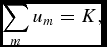
Finally, we define the notion of TU as follows: A set of utility functions satisfy TU if there exists a cardinal representation of each utility such that, for all prices and incomes, the Pareto frontier is a hyperplane of the form
 \begin{equation*}
\sum _{m}u_{m}=K,
\end{equation*}
where K may depend on prices and incomes.
3. A SIMPLE EXAMPLE
We start with a simple example that illustrates our claim. Consider a two-person household consuming two commodities, one that is purely private (the price of which is normalized to 1) and another that can be publicly consumed if two individuals marry.Footnote 7 Individuals are each endowed with some idiosyncratic, exogenous income. We assume that spouses’ respective preferences regarding the private and the public good when married can be represented by the utility function
 \begin{equation}
u_{m}\left( x_{m},X\right) =x_{m}X+\theta _{m}\text{ },\text{\ \ }m=h,\text{ }w\text{,}
\end{equation}
This specification imposes some complementarity between public and private goods. In particular, for this particular, cardinal representation of preferences, the marginal utility from the private good is given by X for both spouses. By construction, it then follows that it is possible to transfer utility within marriage on a one-to-one basis between the spouses, using the private consumption good. In this regard, preference are of the generalized quasi linear (GQL) form described by Bergstrom and Cornes (Reference Bergstrom and Cornes1983).
3.1. Consumption and Utility in Marriage
For the preferences described here, the efficient level of X depends only on its price P and on the aggregate family income y. It is given by
 \begin{equation}
X=\frac{y}{2P}
\end{equation}
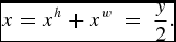
while individual consumptions satisfy
 \begin{equation}
x=x^{h}+x^{w}\text{ }=\text{ }\frac{y}{2}\text{.}
\end{equation}
Note that the consumption of the public good and the aggregate consumption of the private goods both rise with family income. The implied utility levels of the two partners, conditional on the efficient and interior level of the public good, are
 \begin{equation}
U_{m}=x_{m}\frac{y}{2P}+\theta _{m}, \quad m=w,\text{ }h\text{.}
\end{equation}
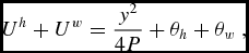
Hence, the Pareto frontier is given by
 \begin{equation}
U^{h}+U^{w}=\frac{y^{2}}{4P}+\theta _{h}+\theta _{w}\text{ ,}
\end{equation}
which defines a straight line with slope − 1. This indicates transferable utility. That is, by shifting the amount of private consumption goods between the two partners, it is possible to transfer utility at a fixed ‘rate of exchange’ that can be normalized to unity.
The significance of this feature is that the new Pareto set generated by any change in circumstances, such as a rise in family income or shocks to marital match quality of either spouse, either includes or is included in the initial Pareto set. In this respect, there is no conflict between the partners in their evaluations of the overall situation that they face—they always prefer the context in which the Pareto set is largest.Footnote 8
3.2. Consumption and Utility in Divorce
Consider, now, the case in which agents decide to divorce. The utilities actually achieved depend on two features.
One is the division of income following divorce, as determined either by law or a private contract between the parties. Without making explicit which of those mechanisms determine the post-divorce allocations, we simply assume that the husband gets βy and the wife gets (1 − β)y for some parameter 0 ⩽ β ⩽ 1.
The other determinant of intra-household welfare is the technology of consumption that prevails after divorce. While the private good certainly remains private, the impact of divorce on consumption of the other (previously public) commodity is less clear. One possibility is that good X is privately consumed after divorce. This would be the case, for instance, of housing, assuming that the spouses quit cohabiting after divorce. Alternatively, the consumption of good X may remain public. For instance, we may think of child utility (or ‘child quality’) as such a good, since parents generally care about their children’s well-being regardless of the state of their marriage. However, divorce may still influence the allocations for this ‘consumption’. A plausible reason for this is that loss of custody or shared custody arrangements reduce the interaction time between at least one of the parents and the child(ren). In essence, this ‘distance’ effect reduces the marginal benefit of child-quality investments.
To capture these ideas in our simple framework, we consider two alternative settings: In one, the public good becomes purely private upon divorce. In the other, the good remains public but the consumption utility of one of the ex-spouses is ‘discounted’ in the sense that the person’s utility is smaller than it was in marriage. Note that, in both cases, we assume that (ordinal) preferences are not modified by divorce—again, the most favorable case for Becker–Coase to hold. We show that, in both cases, condition IER fails to hold. As a result, the Pareto frontiers when married and when divorce may intersect. We then show how the existence of such intersections invalidates the Becker–Coase theorem.
3.2.1. Public good becomes private
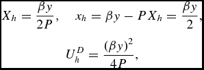
We start with the private consumption case. The ex-husband solves
 \begin{equation}
\max _{x_{h},X_{h}}\left( \beta y-PX_{h}\right) X_{h},
\end{equation}
which yields the consumption levels and the utility
 \begin{eqnarray*}
&\displaystyle X_{h}=\frac{\beta y}{2P},\quad x_{h}=\beta y-PX_{h}=\frac{\beta y}{2}\text{,}&\nonumber \\
&\displaystyle U_{h}^{D}=\frac{\left( \beta y\right) ^{2}}{4P}\text{,} &\nonumber
\end{eqnarray*}
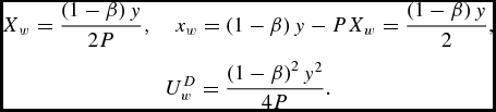
and similarly for the ex-wife
 \begin{eqnarray*}
& \displaystyle X_{w}=\frac{\left( 1-\beta \right) y}{2P},\quad x_{w}=\left( 1-\beta \right) y-PX_{w}=\frac{\left( 1-\beta \right) y}{2}\text{,}& \nonumber \\
& \displaystyle U_{w}^{D}=\frac{\left( 1-\beta \right) ^{2}y^{2}}{4P}\text{.} & \nonumber
\end{eqnarray*}
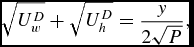
Using transfers, that is, by changing β, it is possible to move along the Pareto frontier in the aftermath of divorce. Specifically, the Pareto frontier in divorce is given by
 \begin{equation}
\sqrt{U_{w}^{D}}+\sqrt{U_{h}^{D}}=\frac{y}{2\sqrt{P}},
\end{equation}
which is decreasing and convex. It is important to note that utilities after divorce still satisfy the TU property, although for a different cardinalization than when married, namely
 \begin{equation*}
\tilde{U}_{w}^{D}=\sqrt{U_{w}^{D}},\quad\tilde{U} _{h}^{D}=\sqrt{U_{h}^{D}}.
\end{equation*}
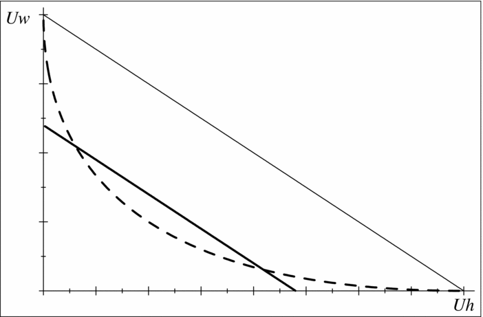
However, this is not sufficient for the Becker–Coase theorem to apply, because it requires that the TU cardinalization be the same in both the married and the divorced states. Indeed, in Figure 1 we compare the Pareto frontiers in marriage and divorce using the same (initial) cardinalization, and assuming that P = 1. The location of the marriage frontier depends on the realization of the θ′s. When θh + θw ⩾ 0, the utility frontier in marriage is completely outside the utility frontier in divorce, because of the economic gains resulting from the joint consumption of public goods when partners live together. Then agents do not divorce. However, variations in θh and θw shift the utility frontier in marriage upwards and downwards. When θh + θw < 0, the two utility frontiers intersect, as indicated by the dashed line.
Pareto frontier in marriage and divorce (with public goods).

Finally, if monotone transformations are applied to individual preferences in marriage and divorce, the shapes of the two Pareto frontiers will change but the pattern of intersections will remain the same.Footnote 9
3.2.2. ‘Distance’ in public consumption
Assume, alternatively, that the marital public goods remain public upon divorce (e.g., ex-spouses still care about the welfare of their offspring). However, the ‘distance’ created by divorce between the non-custodial parent and the child(ren) affects preferences in terms of the relative importance of public and private goods and the evaluation of the marital state compared to being single.
Suppose, for instance, that the mother’s preferences are unaffected by divorce because she maintains custody over the child(ren), but the father’s utility upon divorce becomes
 \begin{equation}
v_{h}\left( x_{h},X\right) =\gamma x_{h}X\text{,}
\end{equation}
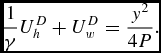
with γ < 1. In words, after divorce, the father’s utility is discounted by some factor γ, compared to its value in marriage. Note that the MRS between private and public consumptions is not affected; we are not assuming that preferences are affected by divorce (which would readily invalidate Becker–Coase), but simply that the level of utility is reduced. Following divorce, and assuming that the provision of public good is still efficient, the Pareto frontier remains therefore linear with a constant (income-independent) slope
 \begin{equation}
\frac{1}{\gamma }U_{h}^{D}+U_{w}^{D}=\frac{y^{2}}{4P}\text{.}
\end{equation}
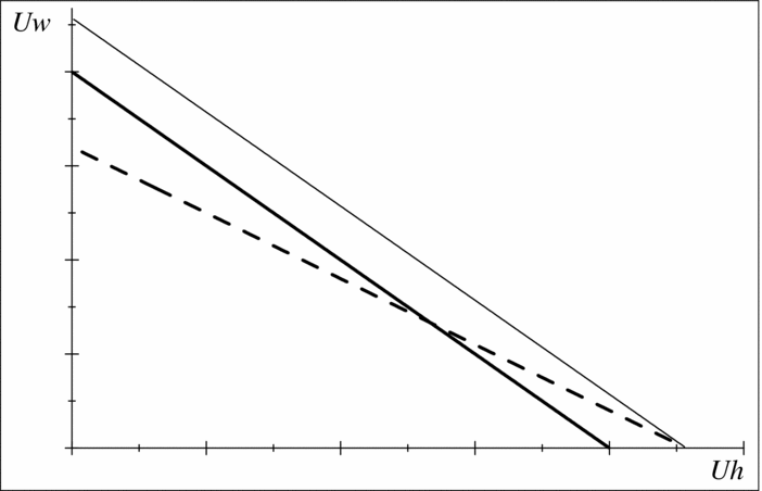
However, the slope is no longer equal to − 1. Instead, it is now − γ > −1, reflecting the father’s ‘discount’ factor in divorce. Figure 2 compares the divorce and marriage frontier in this case. Again, if θh = θw ⩾ 0, the utility frontier in marriage is completely outside the utility frontier in divorce and the divorce frontier upon divorce is steeper because the husband suffers a larger utility loss upon separation. Variations in θh and θw shift the utility frontier in marriage upwards and downwards. But when θh + θw < 0, the two utility frontiers do intersect, as indicated in Figure 2.
Pareto frontier in marriage and divorce (with “distance” in public goods).
3.3. Intersecting Pareto Frontiers and the Becker–Coase theorem
Our key result is that, whenever Pareto frontier under marriage and divorce intersect—including in the two cases described above—the Becker–Coase theorem does not hold; for some realization of the match-quality shocks, the divorce decision depends on the legal framework. In particular, we provide below two examples in which different divorce laws lead to opposite outcomes. The first one is somewhat standard, in the sense that the couple in question would split under unilateral divorce, but would remain married if mutual consent is required. The second example is more counter-intuitive, because the same couple would divorce if mutual consent is required but they would remain married under unilateral divorce. The reason for this is that unilateral divorce would trigger a renegotiation of the intra-household allocations and enable the couple to find efficient reallocations they can agree upon within marriage. We present both examples utilizing the ‘public good becomes private’ framework we worked out above, although the qualitative results would be identical under the “distance” in public consumption setting as well.
3.3.1. Counter-example 1: (Mutual consent reduces divorce)
Consider the case depicted in Figure 1 and suppose that
1. Divorce legislation is rather favorable to men (i.e., β is large; for instance, property is mostly private and the husband is much wealthier than his wife);
2. The realization of the shocks is such that marriage is more valuable to the wife, θw > 0 > θh.
Figure 3 depicts the corresponding points on the Pareto frontiers as M if married and as D if divorced.Footnote 10 One can readily see from the diagram that the couple would remain married if mutual consent is required for divorce. Because of the veto power conferred to either spouse, the wife can guarantee a utility level that is at least equal to what she gets when she is married, namely  $\bar{U}_{w}^{M}$; and no point on the divorce frontier can offer the wife a similar level of welfare without making the husband worse off. Assume, on the contrary, that the husband can unilaterally decide to divorce. Then, he can reach the utility level
 $\bar{U}_{h}^{D}$. This is more than what he can achieve when married and the wife is unable to bribe him to stay. Therefore, the couple would split.Footnote 11
An example of lower divorce likelihood under mutual consent.
The general intuition is clear: whenever the two Pareto frontiers intersect, one can find two utility levels—one for the couple when they are married and another for when they are divorced—such that the wife cannot, under unilateral divorce, ‘bribe’ the husband into staying married and the husband cannot, under mutual consent, payoff his wife to accept separation.
3.3.2. Counter-example 2: (Mutual consent raises divorce)
We now reverse the two assumptions introduced above. In particular, consider the following scenario:
1. Divorce legislation is not too favorable to men (say, it splits household wealth equally between the spouses, β = 1/2);
2. The realization of the shocks favors the husband, θh > 0 > θw.
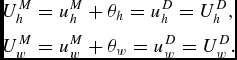
This situation is represented by the Pareto frontiers in Figure 4, where M is the division when the couple remains married and D is the division if the couple divorces. This case is similar to Figure 3 in Clark (Reference Clark1999) and the argument goes as follows. When mutual consent divorce laws apply, the husband will use his veto power to make sure that his utility is at least as much as what he gets when he stays married, namely  $\bar{U}_{h}^{M}$. Therefore, the final outcome must be located to the northeast of point M. Actually, there exist achievable outcomes that Pareto improve upon the current situation. However, they are all located on the divorce frontier. From a straightforward efficiency argument, the partners will renegotiate the divorce contract, allowing them to reach upon divorce a point such as D′, which is preferred by both of them to remaining married.
An example of higher divorce likelihood under mutual consent.
Now consider the case of unilateral divorce. The wife may, by divorcing, achieve the utility level  $\bar{U}_{w}^{D}$ that exceeds her payoff within marriage
 $\bar{U}_{w}^{M}.$ Hence, the initial allocation within marriage, M, is no longer implementable and will be renegotiated. The outcome of the renegotiation must provide the wife with a payoff within marriage that exceeds
 $\bar{U}_{w}^{D}$ and there is a continuum of points on the Pareto frontier when married that are located to the northeast of point D and Pareto dominate the outcome in the case of divorce. Therefore, the couple will remain married and the private consumption goods will be redistributed in favor of the wife to yield an allocation such as M′.
In the first example, the outcomes within marriage and upon divorce that were agreed upon ex-ante (at the time of marriage) are efficient ex-post (after the shocks to the match quality have been realized) and, therefore, are executed. In the second example, these agreements are ex-post inefficient and, therefore, are renegotiated. However, in both cases, the decision ultimately taken is efficient (regardless of whether it is divorce or not) in the conventional sense that no alternative could make both spouses better off. Therefore, a weaker version of the Becker–Coase theorem still holds; outcomes are efficient irrespective of the distribution of property rights. However, it is not generally true that efficiency arguments are sufficient to select a specific decision. On the contrary, there may exist a continuum of different Pareto efficient allocations which correspond to different decisions and outcomes. Efficiency alone cannot determine one particular divorce decision, except in the very peculiar case in which utility remains fully transferable after divorce (i.e., TUD holds, which requires the X commodity to remain public) and the slope of the Pareto frontier is unchanged (i.e., IER holds so that there are no ‘distance’ effects).
In general, whenever one spouse could lose in divorce while the other could gain, there may exist efficient outcomes with and without divorce. And whether or not marriage continues depends on the initial sharing rule, the realization of match-specific qualities and the distribution of property rights as defined by the prevailing divorce legislation.
4. A GENERAL MODEL
We now study the robustness of the insights we sketched out above. We consider a general model of household behavior with an arbitrary number of private and public consumption goods. We provide necessary and sufficient conditions for the Becker–Coase conclusion to hold and then argue that they are unduly restrictive.
Specifically, we show that the requirements for transferable utility within marriage imply that utility cannot be transferable in the aftermath of divorce, at least for the same cardinalization of preferences, except in very specific cases. In practice, while the Bergstrom–Varian conditions for transferable utility within marriage provide a possibly realistic framework for the economic analysis of married couples, they also imply that the three requirements for Becker–Coase to hold are unlikely to be satisfied. This suggests that, in general, divorce laws would impact divorce rates.
4.1. Goods and Preferences
There are n private and N public commodities.Footnote 12 Let xm = (x 1m, . . ., xnm), where m = h, w, denote member m’s private consumption and p = (p 1 = 1, . . ., pn) the corresponding price vector where p 1 is normalized to 1. Similarly, X = (X 1, . . ., XN) denotes the household’s public consumption purchased at price P = (P 1, . . ., PN). Finally, let ym denote member m’s income, ym = yh, yw, and let y = yh + yw be the household’s total (pooled) income.
We assume that utility is transferable between married spouses; clearly, the Becker–Coase intuition cannot apply if this condition is not satisfied. Technically, the transferable utility (TUM) property is satisfied if, for each agent m, there exists a cardinal representation um of m’s preferences such that, for each (p, P), the Pareto set defined by the budget constraint is the hyperplane ∑mum = 1.
Necessary and sufficient conditions for transferability have been derived (see Bergstrom and Cornes Reference Bergstrom and Cornes1983; Bergstrom and Varian 1985; Gugl Reference Gugl2014; Chiappori and Gugl Reference Chiappori and Gugl2014). Specifically, define the conditional indirect utility of agent m as follows:
Definition 1The conditional indirect utility vm is defined by
 \begin{equation}
v_{m}\left( X,p,\rho \right) =\max _{p^{\prime }x=\rho }u_{m}\left( X,x\right).
\end{equation}
In words, vm is the maximal utility agent m can reach when endowed with a vector X of public consumption and an amount ρ to spend on private goods (for the price vector p). We define the conditional demand for private goods, ξm(X, p, ρ), as the solution to (10). Then a necessary and sufficient condition for TUFootnote 13 is that the conditional indirect utility of each member be affine in private expenditures, with the coefficient of private expenditure being the same for all agents. That is, there must exist functions α and βm, m = h, w, homogeneous of respective degree − 1 and 0 in p, such that (for a well-chosen cardinalization)
 \begin{equation}
v_{m}\left( X,p,\rho \right) =\alpha \left( X,p\right) \rho +\beta _{m}\left( X,p\right) ,\quad m=h,\text{ }w\text{.}
\end{equation}
We maintain this assumption throughout the remainder of the paper. Note, incidentally, that this form generates strong testable restrictions. For instance, under TU households behave as if they were maximizing a single utility function; in the language of the theory, they satisfy the unitary representation of household behavior. This implies two types of restrictions for demand functions: they must satisfy Slutsky symmetry and negativeness, and also income pooling, in the sense that observed behavior should depend on aggregate income only, not on its individual components.
A large literature has been devoted to testing these restrictions. Most recent works concentrate on the income pooling property (see, for instance, Thomas Reference Thomas1990; Schultz Reference Schultz1990; Bourguignon et al. Reference Bourguignon, Browning, Chiappori and Lechene1993; Browning et al. Reference Browning, Bourguignon, Chiappori and Lechene1994; Lundberg, Pollak and Wales Reference Lundberg, Pollak and Wales1997; Thomas et al. Reference Thomas, Contreras and Frankenberg1997 and Duflo Reference Duflo2003 to mention just a few). All these papers reject the income pooling assumption. The few contributions testing Slutsky symmetry also reject the property for couples, although, quite interestingly, they fail to reject it for singles (Browning and Chiappori Reference Browning and Chiappori1998; Kapan Reference Kapan2006). These findings suggest that the unitary representation of household behavior, a necessary consequence of the TUM assumption, is far from being an innocuous property, and that it may fail to be supported by the data.
Finally, except for the increase in the number of goods, we maintain all other assumptions on preferences and the timing of events of the simple example presented in Section 2.
4.2. Consumption and Utility in Marriage
Following the standard collective approach (see Chiappori (Reference Chiappori1988, Reference Chiappori1992)), we assume that household decisions are Pareto efficient. As demonstrated elsewhere (for example, Chiappori and Ekeland, Reference Chiappori and Ekeland2009), the decision can be analyzed as a two-stage process. At stage one, the spouses jointly decide the vector of public consumptions, X, and how to split the remaining amount between them. If ρi denotes the amount received by member i (the ‘conditional sharing rule’ in Chiappori and Ekeland’s terms), we have
 \begin{equation}
\rho _{h}+\rho _{w}+\sum _{i}P^{i}X^{i}=y_{h}+y_{w}=y\text{.}
\end{equation}
At the second stage, individuals choose their private consumption vector by maximizing their utility subject to the budget constraint and taking the public consumption vector X as given. The solution to this maximization program is the conditional demand for private goods, ξm(X, p, ρ), and the value of the program is the conditional indirect utility vm(X, p, ρ).
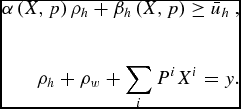
Regarding the first stage, Pareto efficiency implies that the household solves
 \begin{equation}
\max _{\rho _{h},\rho _{w},X}\alpha \left( X,p\right) \rho _{w}+\beta _{w}\left( X,p\right) ,
\end{equation}
under the constraints
 \begin{eqnarray}
\alpha \left( X,p\right) \rho _{h}+\beta _{h}\left( X,p\right) \ge \bar{u}_{h}\text{ ,}\nonumber \\
\\
\rho _{h}+\rho _{w}+\sum _{i}P^{i}X^{i}=y\text{.}\nonumber
\end{eqnarray}
This program satisfies the transferable utility properties. Therefore, the optimal vector X does not depend on the parameter  $\bar{u}_{w}$, and it solves
 \begin{equation}
\max _{X}\alpha \left( X,p\right) \left( y-P^{\prime }X\right) +\beta _{w}\left( X,p\right) +\beta _{h}\left( X,p\right) \text{.}
\end{equation}
Let  $\bar{X}\left( p,P,y\right)$ denote the solution and η(p, P, y) the value of the maximum. Since we do not consider price variations in what follows, we simply write
 $\bar{X}\left( y\right)$ and η(y). The Pareto frontier is the set of couples (UhM, UM w) satisfying the condition
 \begin{equation}
U_{M}^{h}+U_{M}^{w}=\eta \left( y,p,P\right) +\theta _{w}+\theta _{h}\text{.}
\end{equation}
4.3. Consumption and Utility after Divorce
We can now consider the form of individual utilities after divorce. Clearly, if divorce has no impact on either preferences or their cardinal representation, then TUD is a direct consequence of TUM. But such an assumption would clearly be way too restrictive and utterly unrealistic.
Assume, now, that the private or public nature of the various commodities does not change upon divorce, but that the utility they generate is changed. This may be due to changes in preferences themselves (e.g., the marginal rate of substitution between private and public consumption, or between consumption and leisure, is altered by the new situation), or to a different cardinalization (for instance, utility is discounted by some factor, as in the example of Section 2). In the first case, TUD will typically not obtain. In the second, it does, but IER is violated (remember that TU must obtain in marriage and after divorce for the same cardinalization of preferences). We conclude that, in general, the Pareto frontiers in marriage and after divorce do intersect.
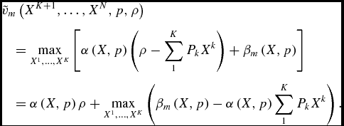
In addition, one may expect that some commodities (housing, heating, landline telephones, and possibly automobiles) are publicly consumed during marriage but become private after divorce. It is interesting to examine how this affects the necessary condition (11). Note, first, that the conditional indirect utilities change. If commodities 1 to K, 1 ⩽ K ⩽ N, become private, then the new conditional indirect utility  $\tilde{v}$ is defined by:
 \begin{equation*}
\tilde{v}_{m}\left( X^{K+1},\ldots ,X^{N},p,\rho \right) =\max _{X^{1},\ldots ,X^{K} }v_{m}\left( X,p,\rho -\sum _{1}^{K}P_{k}X^{k}\right) \text{.}
\end{equation*}
Now, the necessary and sufficient condition for TU is that vm be affine in income. Can we expect the new function  $\tilde{v}_{m}$ to have the same property? The answer is generally negative. Specifically, one can show that
 $\tilde{v}_{m}$ can be affine in ρ in only two cases. One is when the function α(X, p) in (11) does not depend on (X 1, . . ., XK); in that case, indeed,
 \begin{eqnarray*}
&&\tilde{v}_{m}\left( X^{K+1},\ldots ,X^{N},p,\rho \right) \\
&&\quad =\max _{X^{1} ,\ldots ,X^{K}}\left[ \alpha \left( X,p\right) \left( \rho -\sum _{1}^{K} P_{k}X^{k}\right) +\beta _{m}\left( X,p\right) \right] \\
&&\quad =\alpha \left( X,p\right) \rho +\max _{X^{1},\ldots ,X^{K}}\left( \beta _{m}\left( X,p\right) -\alpha \left( X,p\right) \sum _{1}^{K}P_{k} X^{k}\right) \text{.}
\end{eqnarray*}
Note, however, that this case imposes strong (and testable) properties on demand functions. In the particular case K = N, for instance, none of the public good is income elastic: for any interior solution, the demand for public goods only depend on prices, not on income. The extension to the general case K ⩽ N goes as follows. Any change in (P K + 1, . . ., PN, y) that leaves unchanged (X K + 1, . . ., XN) cannot affect X 1, . . ., XK. To see why, note that for any price and income bundle, the optimal level of public consumption X solves
 \begin{equation*}
\max _{X}\alpha \left( X,p\right) \left( y-P^{\prime }X\right) +\beta _{m}\left( X,p\right) \text{.}
\end{equation*}
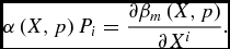
For 1 ⩽ i ⩽ K, first-order conditions give
 \begin{equation*}
\alpha \left( X,p\right) P_{i}=\frac{\partial \beta _{m}\left( X,p\right) }{\partial X^{i}}\text{.}
\end{equation*}
Fix (X K + 1, . . ., XN), then generically the solution to these K equations in K unknowns—namely (X 1, . . ., XK)—is locally unique, and only depends on P 1, . . ., PK.
If, alternatively, α(X, p) depends on Xk for k ⩽ K, then linearity does not obtain unless α and βm satisfy a set of partial differential equations (one for each price-income bundle); again, this condition is generically not satisfied.Footnote 14
We conclude that, in general, there exists values of the shocks such that the Pareto frontiers in marriage and upon divorce intersect. It follows that the situations depicted in  $\emph {Figures}$3 and 4 are fully general; they obtain in the general setting considered in this section as well.
4.4. Extensions
In our framework, a number of generalizations can be introduced at little or no cost. We list the main possible extensions here.
1. Altruism
Although our model assumes ‘egoistic’ preferences, in which individuals care exclusively about their own (public and private) consumption, the extension to more altruistic preferences is straightforward. The key remark, here, is that, as argued for instance by Browning and Chiappori (Reference Browning and Chiappori1998), an allocation that is Pareto efficient for altruistic preferences of the form Wm(uw, uh), h = m, w is Pareto efficient for the egoistic preferences uw, uh. Therefore the collective approach, which only assumes efficiency, readily applies. Assume, furthermore, that the W′s are linear
(17)Then \begin{equation}
W_{m}\left( u_{w},u_{h}\right) =u_{m}+k_{m}u_{n},\;\;n\ne m.
\end{equation}
and the analysis goes through, the slope of the Pareto frontier now being equal to − (1 − kh) / (1 − kw).
\begin{equation*}
\frac{1-k_{w}}{1-k_{w}k_{h}}W_{h}+\frac{1-k_{h}}{1-k_{w}k_{h}}W_{w} =u_{h}+u_{w},
\end{equation*}
Our results are therefore extended in the following way. If, after divorce, either (i) some public commodities become private, or (ii) the utilities are modified, or (iii) the ‘altruism coefficients kh, kw change in such a way that the ratio (1 − kh) / (1 − kw) is modified, then the Becker–Coase theorem does not apply. In particular, (iii) is quite realistic: it is hard to believe that divorce will leave altruistic feelings unchanged between the spouses. We conclude that the introduction of altruism (if anything) strengthens our negative conclusions.
2. Externalities
Our model assumes away consumption externalities, whereby a person’s private consumption directly affects the spouse’s well-being. One issue raised by externalities is the nature of the decision process. Some authors have argued that non-cooperative decision processes should be considered (in which case the Becker–Coase theorem cannot apply). If, on the other hand, one sticks to a cooperative framework (thus assuming that the agents manage to internalize the interaction), then each member’s private consumption of the externality-generating good can be considered as publicly consumed, and the analysis can readily be extended to that case.
3. Non-additive shocks
The exposition of our model is considerably simplified by the separability property of the ‘marriage quality’ shocks. Indeed, the MRS between various commodities are not affected by their realization. Note, however, that nonseparability can only make the three basic properties (TUM, TUD, and IER) more difficult to fulfill. For instance, TUM should hold for any realization of the shocks. Hence, if marital shocks are nonadditive, our result can only be strengthened.
4. Investment
The model presented above contains only consumption activities. Investment activities in schooling or on the job and match-specific investment, such as fertility choices, should be included in any realistic model of the household. The main added element is that the risk of divorce and the type of divorce settlement can affect the shape of the Pareto frontier as well as the sharing rule within marriage. Risk aversion and risk sharing may also become an issue. An analysis of these important issues require a dynamic setup that we have not considered here, but see Rasul (Reference Rasul2006), Matuschek and Rasul (Reference Matouschek and Rasul2006) and Wickelgren (Reference Wickelgren2009) for their treatment.


5. CONCLUDING REMARKS
The Becker–Coase theorem, which is established for an environment without household public goods, posits that changes in divorce laws should have no impact on marriage dissolution rates relies on two main insights. One is that couples will be able to, by bargaining in the shadow of the law, reach Pareto efficient agreements; changes in divorce laws may therefore affect the distribution of the surplus between the spouses, but not the efficiency of the outcome. This intuition remains fully valid in our context. A second ingredient is that only one marital status is compatible with efficiency so that efficiency considerations de facto dictate the divorce decision.
When one extends the original Becker–Coase framework so as to allow household public goods as we do above, the TU assumption is unlikely to hold in both marriage and divorce, at least for the same cardinalization of preferences. As a consequence, the utility frontiers facing a couple upon marriage and divorce can intersect, implying that both marriage and divorce are compatible with efficiency (for different allocations of the property rights). Then, the divorce outcome depends on the initial sharing rule, the realization of match-specific qualities and the distribution of property rights as they are defined by the prevailing divorce legislation. A switch from mutual consent to unilateral may, as expected, increase divorce probability. We show, however, that the opposite effect is also possible. In some circumstances a couple may be more likely to divorce under mutual consent than under unilateral rule. The basic intuition, which in a sense is totally faithful to Becker and Coase’s initial insights, is that the perspective of divorce triggers a renegotiation of the shares, both within marriage and after divorce, from the levels agreed upon at marriage when the quality of match was still unknown; the outcome of such a renegotiation will depend on the exact situation.
Using an explicit model of household consumption and divorce decisions allowed us to derive the testable restrictions implied by transferability in terms of household demand functions. Hence, the choice of a modeling strategy for the analysis of the household (and the marriage market in general) such as transferable utility vs. non-transferable utility can be based on evidence on household behavior rather than on considerations of tractability or faith alone. The available evidence suggests some caution in applying transferable utility, but it is hard to say whether or not we err much by maintaining it as a simplifying assumption for our analysis. In the end, the Becker–Coase theorem, although technically debatable, may remain an acceptable approximation.Footnote 15