1. Introduction
The research on dispersion originated from Taylor’s (Reference Taylor1953) classical analysis of convective–diffusive transport of soluble characteristic of passive substances in laminar flows through a long circular pipe (Wu & Chen Reference Wu and Chen2014). As an important mode of material transport, dispersion plays a key role in fluid mechanics, biophysics (Bees & Croze Reference Bees and Croze2014) and environmental science (Muñoz & Guieysse Reference Muñoz and Guieysse2006; Steinbuck et al. Reference Steinbuck, Stacey, McManus, Cheriton and Ryan2009; Zeng et al. Reference Zeng, Zhang, Wu, Li and Wang2019), among other disciplines. In recent years, a notable research frontier has been emerging to elucidate the mechanisms governing the dispersion of microswimmers and other active particles.
Microswimmers are self-propelled microscopic entities that are ubiquitous in natural and engineered environments. They include naturally occurring microorganisms such as bacteria (Hill et al. Reference Hill, Kalkanci, McMurry and Koser2007; Cisneros et al. Reference Cisneros, Kessler, Ganguly and Goldstein2011; Figueroa-Morales et al. Reference Figueroa-Morales, Rivera, Soto, Lindner, Altshuler and Clément2020), algae (Polin et al. Reference Polin, Tuval, Drescher, Gollub and Goldstein2009; Zeng, Jiang & Pedley Reference Zeng, Jiang and Pedley2022) and ciliates, as well as synthetic micro- and nanoparticles such as self-propelled droplets (Michelin Reference Michelin2023), active Janus particles (Anderson Reference Anderson1989; Jiang, Yoshinaga & Sano Reference Jiang, Yoshinaga and Sano2010; Ghosh et al. Reference Ghosh, Misko, Marchesoni and Nori2013; Moran & Posner Reference Moran and Posner2017) and microrobots (Aghakhani et al. Reference Aghakhani, Yasa, Wrede and Sitti2020; Han et al. Reference Han2024). Unlike passive tracers (Jiang et al. Reference Jiang, Zeng, Fu and Wu2022; Guan & Chen Reference Guan and Chen2024), microswimmers exhibit autonomous motion relative to the surrounding flow, together with rich orientational dynamics, and exhibit complex behaviours in the near-wall region (Lauga & Powers Reference Lauga and Powers2009; Elgeti, Winkler & Gompper Reference Elgeti, Winkler and Gompper2015; Shaebani et al. Reference Shaebani, Wysocki, Winkler, Gompper and Rieger2020). In shear flows they display a variety of intricate accumulation and migration phenomena, including gyrotactic focusing (Kessler Reference Kessler1984, Reference Kessler1985; Pedley & Kessler Reference Pedley and Kessler1992 ), wall accumulation (Rothschild 1963; Berke et al. Reference Berke, Turner, Berg and Lauga2008), shear trapping (Rusconi, Guasto & Stocker Reference Rusconi, Guasto and Stocker2014; Barry et al. Reference Barry, Rusconi, Guasto and Stocker2015; Bearon & Hazel Reference Bearon and Hazel2015; Ezhilan & Saintillan Reference Ezhilan and Saintillan2015; Vennamneni, Nambiar & Subramanian Reference Vennamneni, Nambiar and Subramanian2020), bioconvection (Pedley, Hill & Kessler Reference Pedley, Hill and Kessler1988; Pedley Reference Pedley2010; Hwang & Pedley Reference Hwang and Pedley2014a ) and upstream migration (Hill et al. Reference Hill, Kalkanci, McMurry and Koser2007; Mathijssen et al. Reference Mathijssen, Shendruk, Yeomans and Doostmohammadi2016; Figueroa-Morales et al. Reference Figueroa-Morales, Rivera, Soto, Lindner, Altshuler and Clément2020; Omori et al. Reference Omori, Kikuchi, Schmitz, Pavlovic, Chuang and Ishikawa2022), along with related cross-stream migration behaviours.
To describe and understand the transport processes, several modelling approaches have been developed. Individual-based models (Durham, Climent & Stocker Reference Durham, Climent and Stocker2011; De Lillo et al. Reference De Lillo, Cencini, Durham, Barry, Stocker, Climent and Boffetta2014; Volpe, Gigan & Volpe Reference Volpe, Gigan and Volpe2014; Kumar, Sadekar & Basu Reference Kumar, Sadekar and Basu2020), which capture particle behaviour by directly simulating their paths, are usually formulated from the Langevin equation and run with Brownian dynamics methods. They can handle complicated wall interactions and particle–particle effects. On the downside, they often use a lot of computing resources (Hopkins & Fauci Reference Hopkins and Fauci2002), and the random noise makes the outputs less smooth (Fung, Bearon & Hwang Reference Fung, Bearon and Hwang2022). This can make it harder to see the ‘big-picture’ transport mechanisms. The Pedley–Kessler (PK) model (Pedley & Kessler Reference Pedley and Kessler1990) and the generalised Taylor dispersion (GTD) model (Frankel & Brenner Reference Frankel and Brenner1989; Hill & Bees Reference Hill and Bees2002; Manela & Frankel Reference Manela and Frankel2003) are well-known continuum approaches. They turn microswimmer transport into a standard advection–diffusion problem for the concentration by introducing effective drift speeds and effective dispersion coefficients (Croze et al. Reference Croze, Sardina, Ahmed, Bees and Brandt2013). In doing so, they treat position and orientation as separate. This works in many cases, but for cases with confined spaces it can be with limitations, because they tend to ignore or only roughly treat boundary conditions and near-wall effects (Jiang & Chen Reference Jiang and Chen2020; Fung et al. Reference Fung, Bearon and Hwang2022; Wang, Jiang & Chen Reference Wang, Jiang and Chen2023). Continuum models based on the Smoluchowski equation (Doi & Edwards Reference Doi and Edwards1988) are now mainstream. They describe the full distribution of microswimmers in both physical space and orientation space. The challenge is that the equation is high-dimensional and hard to solve directly (Saintillan & Shelley Reference Saintillan and Shelley2008). To deal with this, some studies use multiple-time-scale methods (Mei, Auriault & Ng Reference Mei, Auriault and Ng1996; Latini & Bernoff Reference Latini and Bernoff2001; Wu & Chen Reference Wu and Chen2014; Vennamneni et al. Reference Vennamneni, Nambiar and Subramanian2020; Guan et al. Reference Guan, Jiang, Tao, Chen and Lee2024; Chen et al. Reference Chen, Jiang, Guo, Zeng and Guan2025) to simplify the problem. The GTD theory (Frankel & Brenner Reference Frankel and Brenner1989; Brenner & Edwards Reference Brenner and Edwards1993) is another useful tool. In this framework, the axial coordinate is treated as the global variable, while the cross-sectional and orientational coordinates are treated as local variables. Combined with the moment method (Aris Reference Aris1956; Chatwin Reference Chatwin1970; Barton Reference Barton1983), it enables a recursive solution for the local statistical moments and has been applied in numerous studies.
In addressing the important problem of microswimmer transport in a pipe flow as the most typical flow mode, many studies have already been carried out (Hwang & Pedley Reference Hwang and Pedley2014b ). Based on the PK model, Bees & Croze (Reference Bees and Croze2010) applied the moment method to study the asymptotic dispersion of concentrated suspensions of gyrotactic microorganisms in vertical pipes, obtaining the effective drift velocity and dispersivity. Bearon, Bees & Croze (Reference Bearon, Bees and Croze2012) employed the GTD framework to analyse the transient dispersion of gyrotactic microorganisms in vertical pipe flow. Croze, Bearon & Bees (Reference Croze, Bearon and Bees2017) conducted fluorescence-labelling experiments to measure the cross-sectional mean drift velocity of algal suspensions in vertical pipe flows, and compared the experimental results with theoretical predictions. Fung, Bearon & Hwang (Reference Fung, Bearon and Hwang2020) investigated the bifurcation and stability of microorganisms, comparing results from the PK and GTD models. Building on the Smoluchowski equation, Jiang & Chen (Reference Jiang and Chen2020) applied GTD theory to solve the asymptotic dispersion of gyrotactic microorganisms in pipe Poiseuille flow, while Guan et al. (Reference Guan, Jiang, Wang, Zeng, Li and Chen2023) further extended the analysis to the corresponding transient dispersion problem. Wang et al. (Reference Wang, Jiang and Chen2023, Reference Wang, Jiang, Zeng and Chen2025) investigated asymptotic dispersion based on the Smoluchowski equation, with consideration of particle–flow interactions.
It is worth emphasising that boundary conditions are among the key factors shaping microswimmer motion and transport in confined spaces, especially in microchannels and in regimes of strong self-propulsion. Experiments show that, near walls, microswimmers exhibit highly complex behaviours: they can accumulate (Rothschild 1963; Berke et al. Reference Berke, Turner, Berg and Lauga2008), slide, undergo specular reflection (Buchner et al. Reference Buchner, Muller, Mehmood and Tam2021) and scatter in a random way (Drescher et al. Reference Drescher, Dunkel, Cisneros, Ganguly and Goldstein2011; Kantsler et al. Reference Kantsler, Dunkel, Polin and Goldstein2013; van Baalen et al. Reference van Baalen, Uspal, Popescu and Isa2023). To model such wall–swimmer interactions, a variety of detailed mechanisms have been proposed, including hydrodynamic interactions, steric effects and biological effects. On the other hand, in theoretical models one often adopts a simpler and more idealised representation by imposing an effective boundary condition for the partial differential equation, which does not explicitly model the microscopic interactions but instead provides an equivalent macroscopic description of their overall effect. In channel flows, there is already much work on specific boundary conditions. For example, Robin conditions (Ezhilan, Alonso-Matilla & Saintillan Reference Ezhilan, Alonso-Matilla and Saintillan2015; Jiang & Chen Reference Jiang and Chen2019; Peng & Brady Reference Peng and Brady2020) are used to represent wall accumulation; specular-reflection conditions (Bearon, Hazel & Thorn Reference Bearon, Hazel and Thorn2011; Volpe et al. Reference Volpe, Gigan and Volpe2014; Ezhilan & Saintillan Reference Ezhilan and Saintillan2015; Jiang & Chen Reference Jiang and Chen2020; Wang, Jiang & Chen Reference Wang, Jiang and Chen2022) to describe regular reflections; and diffuse-reflection conditions (Zeng et al. Reference Zeng, Jiang, Guan, Lee and Chen2025b ) (physically equivalent to the uniformly random reflection considered by Maretvadakethope et al. (Reference Maretvadakethope, Hazel, Vasiev and Bearon2023)) to capture random scattering. Within the continuum framework, boundary conditions not only provide a simplified representation of the physical mechanisms, but also can have a crucial impact on the well-posedness and solvability of the governing partial differential equations. Therefore, their mathematical form often needs to be formulated appropriately, for instance by adopting strengthened conditions or imposing additional mathematical constraints, so that the resulting boundary value problem is well posed and solvable.
Because of higher dimensionality and more complex geometry, problems in pipes are usually harder to analyse, and formulating and implementing boundary conditions for continuum models in a circular pipe are challenging. Boundary conditions that are commonly used in channel flows can become much more difficult to impose in a pipe, and may even be inapplicable. For example, some channel-flow studies avoid prescribing detailed wall conditions by extending the flow field by reflection and then applying periodic boundary conditions (Vennamneni et al. Reference Vennamneni, Nambiar and Subramanian2020; Maretvadakethope et al. Reference Maretvadakethope, Hazel, Vasiev and Bearon2023), but this strategy is difficult to adopt in a circular pipe. Robin conditions, because of their coupled form and the associated high-concentration thin-layer issue, can substantially increase the difficulty of both analytical derivations and numerical computations, especially for pipe problems where the computational cost is already high; consequently, Robin-type conditions have not yet been used in existing theoretical studies of dispersion in circular pipes. Existing work on microswimmers in pipe flows has explored boundary conditions only to a limited extent: theoretical treatments typically consider only specular reflection, or simply neglect wall effects. In addition, many existing models focus either on transient dispersion or on long-time asymptotic dispersion, but only rarely address both together.
In this regard, we set up a theoretical model for microswimmer dispersion in a cylindrical pipe with a diffuse-reflection boundary condition, extending our earlier studies (Jiang & Chen Reference Jiang and Chen2020; Zeng et al. Reference Zeng, Jiang, Guan, Lee and Chen2025b
). We propose an appropriate mathematical formulation of the diffuse-reflection boundary condition in the continuum model for a circular pipe, so as to ensure that the associated Laplacian eigenvalue problem is well posed. This leads to a complete set of basis functions suitable for the Galerkin spectral method, given by products of Bessel functions and spherical harmonics. Because series calculations in a circular pipe are computationally expensive, we simplify the computation by using Wigner
 $3j$
symbols to evaluate the integrals involving products of spherical harmonics. The long-time asymptotic and transient solutions of the moments are obtained by combining GTD theory and a bi-orthogonal expansion, respectively. The resulting framework enables us to systematically describe and analyse, over the entire transport process, the evolution of the local and radial distributions, the drift velocity and the dispersivity, and to examine how key parameters shape the evolution of these quantities. This study primarily focuses on the regime of large swimming Péclet numbers and is more relevant to artificial microswimmers, for which specific control can be more readily implemented. This work helps fill the knowledge gap associated with boundary conditions in circular pipes and provides a foundation for future studies of more complex and refined boundary conditions.
The structure of the paper is as follows. Section 2 introduces the transport problem of microswimmers under diffuse-reflection boundary conditions in a vertical pipe flow and specifies the initial conditions. In § 3, we use the moment method to convert the transport equation into moment equations and then apply GTD theory together with a Galerkin spectral method to obtain the asymptotic solutions for the moments. The basic functions of the spectral method are constructed by analytically deriving eigenfunctions of the Laplace operator under diffuse-reflection boundary conditions. Section 4 examines the local distribution and investigates how swimming speed, gyrotactic strength, shape factor, translational diffusivity and the direction and strength of shear flow affect the asymptotic radial distribution, as well as the temporal evolution of the transient radial distribution. Section 5 analyses the influence of these key parameters on the dispersion coefficients, including the drift velocity and dispersivity, and further characterises the time histories of the transient drift and dispersivity. Conclusions and outlook are given in § 6. Appendix A presents the bi-orthogonal expansion method used to solve the transient moments.
2. Formulation
2.1. Governing equations
Sketch of a dilute suspension of ellipsoidal microswimmers in a vertical downwelling pipe flow. (a) Flow profile and cylindrical coordinate system. (b) Definition of orientation angles. (c) Schematic of diffuse reflection (left) and specular reflection (right) at the pipe wall.

As illustrated in figure 1, we consider the dispersion process of a dilute suspension of microswimmers in a vertical cylindrical pipe flow. The pipe has a radius denoted by
 $R^*$
, where the superscript
 $\ast$
denotes dimensional quantities. To describe the microswimmers’ positions in space, we adopt a cylindrical coordinate system
 $(r^*, \psi , z^*)$
, with corresponding unit vectors
 $\boldsymbol{e}_r$
,
 $\boldsymbol{e}_\psi$
and
 $\boldsymbol{e}_z$
. The background flow is assumed to be steady, unidirectional and axisymmetric, given by
 $\boldsymbol{U}^* = U^*(r^*) \boldsymbol{e}_z$
, where
 $U^*(r^*)$
denotes the axial flow speed as a function of the radial coordinate.
Characterising the swimming orientation of the particles, we use a spherical coordinate system
 $(\rho , \theta , \phi )$
, along with the associated unit vectors
 $\boldsymbol{e}_\rho$
,
 $\boldsymbol{e}_\theta$
and
 $\boldsymbol{e}_\phi$
. Here,
 $\theta$
is the polar (zenith) angle, defined as the angle between the swimming direction vector
 $\boldsymbol{p}$
and the azimuthal unit vector
 $\boldsymbol{e}_\psi$
;
 $\phi$
is the azimuthal angle, defined as the angle between
 $-\boldsymbol{e}_z$
and the projection of
 $\boldsymbol{p}$
onto the
 $O z^* r^*$
plane. The swimming direction vector can thus be expressed as
 \begin{equation} \boldsymbol{p} = \boldsymbol{e}_{\rho } = p_r(\theta , \phi )\, \boldsymbol{e}_r + p_{\psi }(\theta , \phi )\, \boldsymbol{e}_{\psi } + p_z(\theta , \phi )\, \boldsymbol{e}_z, \end{equation}
where
 \begin{equation} p_r = -\sin \theta \sin \phi , \quad p_{\psi } = \cos \theta , \quad p_z = -\sin \theta \cos \phi . \end{equation}
The dimensionless parameters are defined as follows:
 \begin{equation} \left \{ \begin{aligned} t &= t^* D_r^*, \quad r = \frac {r^*}{R^*}, \quad z = \frac {z^*- U_m^*\, t^*}{R^*}, \quad U = \frac {U^*}{U_m^*} - 1, \\ \textit{Pe}_s &= \frac {V_s^*}{D_r^* R^*}, \quad \textit{Pe}_{\!f} = \frac {U_m^*}{D_r^* R^*}, \quad D_t = \frac {D_t^*}{D_r^* R^{*2}}, \quad \lambda = \frac {1}{2 B^* D_r^*}, \end{aligned} \right . \end{equation}
where
 $t^{\ast }$
is the time;
 $V_s^{\ast }$
is the constant swimming speed of the microswimmers;
 $D_t^{\ast }$
and
 $D_r^{\ast }$
represent the randomness in microswimmers’ position and orientation resulting from biological variation in their motility, including both thermal and athermal sources (Drescher et al. Reference Drescher, Dunkel, Cisneros, Ganguly and Goldstein2011; Garcia et al. Reference Garcia, Berti, Peyla and Rafaï2011);
 $B^*$
is the gravitactic reorientation time quantifying the balance between hydrodynamic torque and viscous resistance; and
 $U_m^*$
is the average flow velocity given as
 \begin{equation} U_m^* \triangleq \frac {1}{{R^*}^2} \int _0^{R^*} 2r^*U^*(r^*) \, \mathrm{d} r^*. \end{equation}
Here,
 $\textit{Pe}_s$
is the swimming Péclet number characterising the swimming ability relative to the pipe diameter and rotational diffusion, or equivalently the degree of confinement;
 $\textit{Pe}_{\!f}$
is the flow Péclet number representing the overall strength and velocity of the shear flow;
 $D_t$
is the ratio of translational diffusion decorrelation time scale to rotational diffusion reorientation time scale; and
 $\lambda$
is the dimensionless inverse of the gravitactic time scale
 $B^{\ast }$
.
We assume that the suspension of microswimmers is dilute enough to neglect their mutual interactions as well as their impact on the background flow (e.g. concentration much less than
 $1 \times 10^6 \textrm{cells cm}^{-3}$
for microswimmers with diameters less than
 $10$
μm) (Croze et al. Reference Croze, Bearon and Bees2017; Bees Reference Bees2020). The evolution of the probability density function for the microswimmer population can be described by the dimensionless form of the Smoluchowski equation (Doi & Edwards Reference Doi and Edwards1988):
 \begin{equation} \frac {\partial P}{\partial t} + \boldsymbol{\nabla }_{\!R} \boldsymbol{\cdot }\left [ \left ( \textit{Pe}_{\!f} U \boldsymbol{e}_z + \textit{Pe}_s \boldsymbol{p} \right ) P - D_t \boldsymbol{\nabla }_{\!R} P \right ] + \boldsymbol{\nabla }_{\!p} \boldsymbol{\cdot }\left ( \dot {\boldsymbol{p}_r} P - \boldsymbol{\nabla }_{\!p} P \right ) = 0, \end{equation}
where
 $P$
is the probability of finding a microswimmer at the position-and-orientation point
 $(r,\psi ,z,\theta ,\phi )$
at time
 $t$
;
 $\boldsymbol{\nabla }_{\!R}$
and
 $\boldsymbol{\nabla }_{\!p}$
are defined as the gradient operator
 $\boldsymbol{\nabla }_{\!R} = \boldsymbol{e}_r ({\partial }/{\partial r}) + \boldsymbol{e}_{\psi } ( {1}/{r})( {\partial }/{\partial \psi }) + \boldsymbol{e}_z ( {\partial }/{\partial z}),$
and
 $\boldsymbol{\nabla }_{\!p} = \boldsymbol{e}_{\theta } ({\partial }/{\partial \theta }) + \boldsymbol{e}_{\phi }( {1}/{\sin \theta })({\partial }/{\partial \phi })$
in the position and orientation space;
 $U(r)$
is the velocity of the shear flow; and
 $\dot {\boldsymbol{p}_r}$
is the relative rate of change of swimming direction
 \begin{equation} \dot {\boldsymbol{p}}_r = \dot {\boldsymbol{p}} - \dot {\boldsymbol{p}}_c, \end{equation}
where
 $\dot {\boldsymbol{p}}$
is the rate of change of swimming direction governed by the Jeffery equation, with gyrotaxis taken into account (Jeffery & Filon Reference Jeffery and Filon1922; Hinch & Leal Reference Hinch and Leal1972; Pedley & Kessler Reference Pedley and Kessler1992):
 \begin{equation} \dot {\boldsymbol{p}} = -\lambda \;\boldsymbol{p} \times \boldsymbol{e}_z \times \boldsymbol{p}+ \frac {1}{2} \textit{Pe}_{\!f}\boldsymbol{\omega } \times \boldsymbol{p}+\textit{Pe}_{\!f}\alpha _0 [\boldsymbol{p} \times (\boldsymbol{E}\boldsymbol{\cdot } \boldsymbol{p})] \times \boldsymbol{p}, \end{equation}
where
 $\boldsymbol{\omega } = \boldsymbol{\nabla }_{\!R} \times \boldsymbol{U}$
and
 $\boldsymbol{E} =({1}/{2}) [\boldsymbol{\nabla }_{\!R} \boldsymbol{U} +(\boldsymbol{\nabla }_{\!R} \boldsymbol{U})^{{T}} ]$
are the vorticity and rate-of-strain tensor of the flow and
 $\alpha _0$
is the shape factor of the microswimmer ranging from
 $0$
(spherical) to
 $1$
(rod-like). Specifically,
 $\dot {\boldsymbol{p}}_c$
emerges due to the swimming of a microswimmer in the
 $\boldsymbol{e}_{\psi }$
direction and the dependence of spherical coordinate characterising the orientation of the microswimmer on the cylindrical coordinate fixed in position space. The angular velocity of the rotating spherical coordinate is
 $(\textit{Pe}_{\!s}{\cos \theta }/{r})\boldsymbol{e}_z \times \boldsymbol{p}$
. The detailed expression of
 $\dot {\boldsymbol{p}}_r$
is
 \begin{equation} \dot {\boldsymbol{p}}_r = \dot {\theta } \, \boldsymbol{e}_{\theta } + \dot {\phi } \sin \theta \, \boldsymbol{e}_{\phi }, \end{equation}
in which the two angular velocity change rates in the swimming direction are
 \begin{align} &\dot {\theta } = \lambda \cos \phi \cos \theta + \frac {\alpha _0 \textit{Pe}_{\!f}}{4} \frac {\partial U}{\partial r} \sin 2\theta \sin 2\phi - \frac {\textit{Pe}_s}{r} \cos \theta \sin \phi , \\[-12pt]\nonumber\end{align}
 \begin{align} &\dot {\phi } = -\lambda \frac {\sin \phi }{\sin \theta } - \frac {\textit{Pe}_{\!f}}{2} \frac {\partial U}{\partial r} \left ( 1 - \alpha _0 \cos 2\phi \right ) - \frac {\textit{Pe}_s}{r} \cos \theta \cot \theta \cos \phi . \end{align}
We consider the classical laminar Poiseuille flow in a circular pipe; neglecting the influence of microswimmers on the flow, in a frame moving with the mean flow, the dimensionless velocity profile is given as
 \begin{equation} U(r)=1-2r^2. \end{equation}
2.2. Boundary condition and initial condition
Boundary conditions significantly influence the transport processes of microswimmers within confined geometries (Berke et al. Reference Berke, Turner, Berg and Lauga2008; Bianchi et al. Reference Bianchi, Saglimbeni, Frangipane, Dell’Arciprete and Leonardo2019; Buchner et al. Reference Buchner, Muller, Mehmood and Tam2021). In this study, we focus specifically on diffuse reflection boundary conditions applied to a cylindrical pipe flow. Microswimmers are assumed to undergo random reorientation upon encountering the pipe wall, with the reflected orientations uniformly distributed over all possible directions (similar to the diffuse-reflection principle of light), as shown in figure 1(c). Unlike the case of a two-dimensional channel (Maretvadakethope et al. Reference Maretvadakethope, Hazel, Vasiev and Bearon2023; Zeng et al. Reference Zeng, Jiang, Guan, Lee and Chen2025b ), the reflection angles in a cylindrical pipe involve one additional degree of freedom. Additionally, we assume that this diffuse reflection occurs instantaneously, neglecting any finite residence time or interaction duration of microswimmers at the boundary. Such diffuse boundary conditions can capture the random scattering behaviour of microswimmers near walls and provide boundary effects distinct from specular reflection.
In reality, near-wall swimming behaviour of real microswimmers can be highly complex and may involve sticking, sliding or partial reorientation. Some experiments have observed that (Cisneros et al. Reference Cisneros, Kessler, Ganguly and Goldstein2011; Kantsler et al. Reference Kantsler, Dunkel, Polin and Goldstein2013; Contino et al. Reference Contino, Lushi, Tuval, Kantsler and Polin2015), upon wall encounters, both bacteria and microalgae can exhibit scattering behaviours, with outgoing angles that may be essentially uncorrelated with the incoming angles (random scattering) or, alternatively, correlated with the incoming angles and following a prescribed distribution. In comparison, the diffuse-reflection boundary condition adopted here is an idealised case, representing completely random reorientation with uniformly distributed reflection angles. Nevertheless, such a condition serves as a useful theoretical approximation and provides an equivalent macroscopic description of the overall effect of wall encounters. This idealisation is more relevant to engineered synthetic systems, including active Janus particles (van Baalen et al. Reference van Baalen, Uspal, Popescu and Isa2023) and microrobots, for which a diffuse-reflection-type response can be approximately realised through tailored surface designs or active control strategies.
The following mathematical form of the boundary condition is introduced in the continuum model:
 \begin{align} \left \{ \begin{aligned} \frac {\partial P}{\partial \theta }(r, \psi , z, \theta , \phi , t) &= 0 \quad \text{at } \quad r = 1, \\ \frac {\partial P}{\partial \phi }(r, \psi , z, \theta , \phi , t) &= 0 \quad \text{at } \quad r = 1. \end{aligned} \right . \end{align}
Note that this boundary condition is a mathematically stronger variant of diffuse reflection. We adopt the form to ensure the solvability and uniqueness of the eigenfunction problem under this boundary condition (see § 3.3.1 for details). Such a strengthening is a commonly adopted approach in theoretical analyses and has been widely used in previous work (Bearon et al. Reference Bearon, Hazel and Thorn2011; Bearon & Hazel Reference Bearon and Hazel2015; Ezhilan et al. Reference Ezhilan, Alonso-Matilla and Saintillan2015; Jiang & Chen Reference Jiang and Chen2019; Zeng et al. Reference Zeng, Jiang, Guan, Lee and Chen2025b ).
In addition, to ensure conservation of the total number of microswimmers, a zero-flux condition (Ezhilan, Pahlavan & Saintillan Reference Ezhilan, Pahlavan and Saintillan2012; Bearon & Hazel Reference Bearon and Hazel2015) is imposed at the boundary:
 \begin{align} \begin{aligned} 0=\int _0^{\pi }\int _0^{2\pi } (\boldsymbol{e}_r \boldsymbol{\cdot }\boldsymbol{J}_{\!R})\, \sin \theta \, \mathrm{d}\phi \, \mathrm{d}\theta = \int _{0}^{\pi } \int _0^{2\pi } \left ( - \textit{Pe}_s \sin \theta \sin \phi \, P - D_t \frac {\partial P}{\partial r} \right ) \sin \theta \, \mathrm{d}\phi \, \mathrm{d}\theta \\ \quad \mathrm{at} \; r = 1, \end{aligned} \end{align}
where
 $\boldsymbol{J}_{\!R} = [\textit{Pe}_{\!f}U(r)\boldsymbol{e}_z+\textit{Pe}_s\boldsymbol{p} ]P-D_t {\boldsymbol{\nabla }}_{\!R}P$
is the position-space flux of microswimmers. The first term on the right-hand side of the equation denotes the advective flux due to swimming, which vanishes under the diffuse-reflection condition (2.12). The second term represents the diffusive flux, projected in the direction normal to the wall, which must also vanish and can therefore be simplified to the following expression:
 \begin{equation} \int _{0}^{\pi } \int _0^{2\pi } \, \frac {\partial P}{\partial r} \, \sin \theta \, \mathrm{d}\phi \, \mathrm{d}\theta = 0 \quad \mathrm{at} \; r = 1. \end{equation}
At the centre of the cylindrical pipe (
 $r=0$
), the probability distribution function is required to remain bounded:
 \begin{equation} P \big |_{r=0} \ne \infty . \end{equation}
Periodic boundary condition is imposed in the azimuthal direction
 $\psi$
:
 \begin{equation} \begin{aligned} P \big |_{\psi = 0} = P \big |_{\psi = 2\pi }, \; \left . \frac {\partial P}{\partial \psi } \right |_{\psi = 0} = \left . \frac {\partial P}{\partial \psi } \right |_{\psi = 2\pi }. \end{aligned} \end{equation}
In the swimming direction space, the probability distribution function is required to remain bounded:
 \begin{equation} P \big |_{\theta = 0} \ne \infty , \quad P \big |_{\theta = \pi } \ne \infty . \end{equation}
Periodic boundary condition for
 $\phi$
is given by
 \begin{equation} \begin{aligned} P \big |_{\phi = 0} = P \big |_{\phi = 2\pi }, \; \left . \frac {\partial P}{\partial \phi } \right |_{\phi = 0} = \left . \frac {\partial P}{\partial \phi } \right |_{\phi = 2\pi }. \end{aligned} \end{equation}
The normalisation condition is given as
 \begin{equation} \int ^{\infty }_{-\infty } \langle P \rangle \, \mathrm{d}z= 1, \end{equation}
where the operator
 $\langle \boldsymbol{\cdot }\rangle$
is defined to represent the local spatial averaging
 \begin{align} \langle \boldsymbol{\cdot }\rangle \triangleq \int _{0}^{1}\int _{0}^{2\pi }\int _{0}^{\pi }\int _{0}^{2\pi } (\boldsymbol{\cdot })\, r\sin \theta \,\mathrm{d}\phi \,\mathrm{d}\theta \,\mathrm{d}\psi \,\mathrm{d}r. \end{align}
For the long-time asymptotic problem, the specification of an explicit initial condition is not required, whereas for the transient problem an initial condition must be prescribed. The initial condition for
 $P$
is taken as
 \begin{equation} P \big |_{t = 0} = \frac {1}{2\pi }\delta (z) P^{(0)}(r,\theta ,\phi ), \end{equation}
where
 $\delta$
is the Dirac delta function and
 $P^{(0)}$
is a specific probability distribution function. In this work, we consider an instantaneous release of microswimmers at
 $z=0$
, with the distribution being axisymmetric, i.e. uniform with respect to the azimuthal angle
 $\psi$
.
Furthermore, we assume that the swimmers are initially released with a uniform distribution over the cross-section and in the swimming-direction space, corresponding to random position and orientation. This is represented by
 \begin{equation} P^{(0)}(r,\theta ,\phi ) = \frac {1}{2\pi }. \end{equation}
3. Solution
3.1. Local and global spaces
According to the GTD theory (Frankel & Brenner Reference Frankel and Brenner1989; Brenner & Edwards Reference Brenner and Edwards1993), the entire position–orientation space can be partitioned into a global space and a local space. The global space is defined by the longitudinal (streamwise) coordinate
 $z$
, while the local space consists of the cross-sectional coordinates
 $(r,\psi )$
together with the orientation variables
 $(\theta ,\phi )$
. Based on the division of global and local spaces, the dimensionless form of the probability conservation can be written as
 \begin{equation} \frac {\partial P}{\partial t} + \left [ \textit{Pe}_{\!f} U(r) - \textit{Pe}_s \sin \theta \cos \phi \right ] \frac {\partial P}{\partial z} - D_t \frac {\partial ^2 P}{\partial z^2} = \mathcal{L}_0 P , \end{equation}
where
 $\mathcal{L}_0$
is defined in local space:
 \begin{equation} \begin{aligned} \mathcal{L}_0 P \triangleq \ & D_t \left [ \frac {1}{r} \frac {\partial }{\partial r} \left ( r \frac {\partial P}{\partial r} \right ) + \frac {1}{r^2} \frac {\partial ^2 P}{\partial \psi ^2} \right ] + \frac {\textit{Pe}_s \sin \theta \sin \phi }{r} \frac {\partial (rP)}{\partial r} - \frac {\textit{Pe}_s \cos \theta }{r} \frac {\partial P}{\partial \psi } \\ & - \frac {1}{\sin \theta } \frac {\partial }{\partial \theta } (\dot {\theta } \sin \theta P) - \frac {\partial (\dot {\phi } P)}{\partial \phi } + \frac {1}{\sin \theta } \frac {\partial }{\partial \theta } \left ( \sin \theta \frac {\partial P}{\partial \theta } \right ) + \frac {1}{\sin ^2\theta } \frac {\partial ^2 P}{\partial \phi ^2}. \end{aligned} \end{equation}
Because the pipe geometry, base flow and boundary conditions are axisymmetric, that is, unchanged under rotations about the axis, the governing problem is invariant in the azimuthal direction. We therefore assume
 $P$
is independent of the azimuthal angle
 $\psi$
(so
 $\partial _{\psi }P=0$
), under which the operator
 $\mathcal{L}_0$
reduces to the following form:
 \begin{equation} \begin{aligned} \mathcal{L} P \triangleq \ & D_t\frac {1}{r} \frac {\partial }{\partial r} \left ( r \frac {\partial P}{\partial r} \right ) + \frac {\textit{Pe}_s \sin \theta \sin \phi }{r} \frac {\partial (rP)}{\partial r} - \frac {1}{\sin \theta } \frac {\partial }{\partial \theta } (\dot {\theta } \sin \theta P) \\ &- \frac {\partial (\dot {\phi } P)}{\partial \phi } + \frac {1}{\sin \theta } \frac {\partial }{\partial \theta } \left ( \sin \theta \frac {\partial P}{\partial \theta } \right ) + \frac {1}{\sin ^2\theta } \frac {\partial ^2 P}{\partial \phi ^2}. \end{aligned} \end{equation}
From this point on, we write
 $P = P(r, z, \theta , \phi , t)$
, and the azimuthal variable
 $\psi$
is used only when applying the normalisation condition.
3.2. Moment equation
The moment method provides an efficient approach for extracting macroscopic transport information by converting the Smoluchowski equation into a reduced set of moment equations. The central premise of this technique is to quantify the statistical characteristics of the particle distribution by computing its integral moments with respect to selected variables. These calculated moments then serve as a simplified yet complete representation of the overall dynamics and macroscopic properties of the particle population.
The local moments and total moments are defined as follows (Aris Reference Aris1956; Smith Reference Smith1985; Bees & Croze Reference Bees and Croze2010):
 \begin{equation} P_n(r, \theta , \phi , t) \triangleq \int _{-\infty }^{\infty } z^n P(r, z, \theta , \phi , t) \, \mathrm{d}z, \quad n = 0, 1, \ldots , \end{equation}
 \begin{equation} M_n(t) \triangleq \int _{-\infty }^{\infty } z^n \langle P \rangle \, \mathrm{d}z, \quad n = 0, 1, \ldots\ . \end{equation}
With the assumption that concentration decays exponentially as
 $|z| \to \infty$
(Aris Reference Aris1956; Chatwin Reference Chatwin1970), multiplying the governing equation by
 $z^n$
and integrating over
 $z \in (-\infty ,\infty )$
, we get the following governing equations for
 $n$
-order local moments
 $P_n$
:
 \begin{equation} \begin{aligned} \frac {\partial P_n}{\partial t} = n(n-1) D_t P_{n-2} + n (\textit{Pe}_{\!f} U - \textit{Pe}_s \sin \theta \cos \phi ) P_{n-1} + \mathcal{L} P_n, \quad n=0,1,\ldots\ . \end{aligned} \end{equation}
Here
 $P_{-1}=P_{-2}=0$
is introduced to unify the form of all moment equations.
Integrating (3.6) over the local space, we can obtain the governing equation for the global moment:
 \begin{align} \frac {\mathrm{d} M_n}{\mathrm{d} t} = n(n-1) D_t M_{n-2} + n \langle \left ( \textit{Pe}_{\!f} U - \textit{Pe}_s \sin \theta \cos \phi \right ) P_{n-1} \rangle , \end{align}
where
 $n = 0,1, \ldots$
. Due to the zero-flux boundary condition (2.13) and the periodic condition (2.18), the contribution from the operator
 $\mathcal{L}$
vanishes upon integration over the local space.
3.3. Solution of radial distribution
The zeroth-order moment corresponds to the marginal distribution of microswimmers in the local space, and its governing equation is given by (3.6) with
 $n=0$
:
 \begin{equation} \begin{aligned} \frac {\partial P_0}{\partial t} = \mathcal{L} P_0 . \end{aligned} \end{equation}
The long-time asymptotic state of the zeroth-order local moment
 $P_0$
is defined as
 \begin{equation} P_0^{\infty }(r, \theta , \phi ) \triangleq \lim _{t \to \infty } P_0(r, \theta , \phi , t) . \end{equation}
According to the GTD theory, the solution of
 $P^{\infty }_0$
satisfies
 \begin{equation} \mathcal{L} P_0^{\infty } = 0. \end{equation}
The boundary conditions of
 $P_0$
and
 $P_0^\infty$
are the same as those of
 $P$
, and they are further required to satisfy the normalisation conditions
 $\langle P_0 \rangle =1$
and
 $\langle P_0^\infty \rangle =1$
.
According to the obtained zeroth-order moment, we define the asymptotic radial distribution of longitudinally and orientationally accumulated concentration (hereafter abbreviated as asymptotic radial distribution or simply radial distribution) and transient radial distribution of longitudinally and orientationally accumulated concentration (hereafter abbreviated as transient radial distribution) as follows:
 \begin{equation} C_r(r) \triangleq \int _0^{\pi } \int _0^{2\pi } P_0^{\infty }(r, \theta , \phi ) \sin \theta \,\mathrm{d}\phi \, \mathrm{d}\theta , \end{equation}
 \begin{equation} C_t(r,t) \triangleq \int _0^{\pi } \int _0^{2\pi } P_0(r, \theta , \phi , t) \sin \theta \,\mathrm{d}\phi \, \mathrm{d}\theta , \end{equation}
which serve to characterise and clarify the migration dynamics and spatial distribution patterns of microswimmers.
Due to the active swimming terms contained in the operator
 $\mathcal{L}$
, the operator is non-self-adjoint, which makes classical mathematical techniques such as separation of variables inapplicable. To address this, we employ a Galerkin spectral method (Doi & Edwards Reference Doi and Edwards1978; Hill & Bees Reference Hill and Bees2002; Manela & Frankel Reference Manela and Frankel2003) to approximate the solution of the homogeneous elliptic partial differential equation (3.10). Specifically, we analytically derive the eigenfunctions of the generalised Laplace operator under all relevant boundary conditions and use them to construct a basis set for the spectral method. Additionally, to treat the transient problem (3.8), we further combine this approach with a bi-orthogonal eigenfunction expansion; the detailed procedure is provided in Appendix A.
3.3.1. Orthogonal and complete basis functions
To apply the Galerkin spectral method, we require a complete set of basis functions in the local space, which can be constructed from the eigenfunctions of the generalised Laplace operator. Specifically, the generalised Laplace operator under consideration is defined as follows:
 \begin{equation} \varDelta = \frac {1}{r} \frac {\partial }{\partial r} \left ( r \frac {\partial }{\partial r} \right ) + \frac {1}{\sin \theta } \frac {\partial }{\partial \theta } \left ( \sin \theta \frac {\partial }{\partial \theta } \right ) + \frac {1}{\sin ^2\theta } \frac {\partial ^2}{\partial \phi ^2}. \end{equation}
The eigenfunctions are derived by solving the eigenvalue problem:
 \begin{equation} -\!\Delta f = \lambda f, \quad (r,\theta ,\phi ) \in [0,1]\times [0,\pi ]\times [0,2\pi ], \end{equation}
with the boundary conditions
 \begin{align} &\frac {\partial f}{\partial \theta } = 0 \quad \text{at } \quad r = 1, \\[-12pt]\nonumber\end{align}
 \begin{align} &\frac {\partial f}{\partial \phi } = 0 \quad \text{at } \quad r = 1, \\[-12pt]\nonumber \end{align}
 \begin{align} &\int _{0}^{\pi } \int _0^{2\pi } \, \frac {\partial f}{\partial r} \, \sin \theta \, \mathrm{d}\phi \, \mathrm{d}\theta = 0 \quad \mathrm{at} \quad r = 1, \\[-12pt]\nonumber \end{align}
 \begin{align} &f \big |_{r=0} \ne \infty , \\[-12pt]\nonumber \end{align}
 \begin{align} &f \big |_{\theta = 0} \ne \infty , \quad f \big |_{\theta = \pi } \ne \infty , \\[-12pt]\nonumber\end{align}
 \begin{align} &f \big |_{\phi = 0} = f \big |_{\phi = 2\pi }, \quad \left . \frac {\partial f}{\partial \phi } \right |_{\phi = 0} = \left . \frac {\partial f}{\partial \phi } \right |_{\phi = 2\pi },\end{align}
and the normalisation condition
 \begin{equation} \int _0^1 \int _0^{\pi } \int _0^{2\pi } \left |f\right |^2 \, r \, \sin \theta \, \mathrm{d}\phi \, \mathrm{d}\theta \, \mathrm{d}r = 1. \end{equation}
Because the Laplace operator is separable, we can write the eigenfunction as a product of a radial part
 $R(r)$
and an angular part
 $Y_l^{m}(\theta ,\phi )$
:
 \begin{equation} f(r,\theta ,\phi ) = R(r) Y_l^m(\theta ,\phi ). \end{equation}
Here the angular part is governed by the associated Legendre equation, subject to the regularity conditions (3.19) at the poles (
 $\theta =0,\pi$
) and the periodic conditions (3.20) in the azimuthal direction. Its solutions are the spherical harmonics, which in the normalised form are given by
 \begin{equation} Y_l^m(\theta , \phi ) = \sqrt {\frac {2l + 1}{4\pi }\frac {(l - m)!}{(l + m)!}} P_l^m(\cos \theta ){\rm e}^{{\rm i}m\phi }, \end{equation}
with
 $l=0,1,2,\ldots$
and
 $m=0,1,\ldots ,l$
, where the associated Legendre functions
 $P_l^m(x)$
are defined by
 \begin{equation} P_l^m(x) = (-1)^m(1 - x^2)^{m/2}\frac {{d}^m}{\mathrm{d}x^m}P_l(x). \end{equation}
The radial part satisfies the zero-order Bessel equation:
 \begin{equation} \frac {1}{r}\frac {{d}}{\mathrm{d}r}\left (r\frac {\mathrm{d}R}{\mathrm{d}r}\right ) - l(l+1)R + \lambda R = 0. \end{equation}
Due to the regularity condition (3.18) at
 $r=0$
, the solution reduces to the Bessel function of the first kind only. Then we analytically derive the solution of
 $R(r)$
based on the different cases of the angle part.
(i) Case
 $l=0$
For this case, we have
 \begin{equation} Y_0^0(\theta ,\phi )=\frac {1}{2\sqrt {\pi }}, \end{equation}
which indicates that the corresponding eigenfunction
 $f$
is independent of both the polar angle
 $\theta$
and the azimuthal angle
 $\phi$
, i.e.
 \begin{equation} \frac {\partial f}{\partial \theta } = 0, \quad \frac {\partial f}{\partial \phi } = 0. \end{equation}
So the conditions (3.15) and (3.16) are automatically satisfied, and the condition (3.17) is required to satisfy the following mathematical form:
 \begin{equation} 0=\int _0^{\pi } \int _{0}^{2\pi } \sin \theta \,\left .\frac {\partial f}{\partial r}\right |_{r=1} \,\mathrm{d}\phi \,\mathrm{d}\theta = \int _0^{\pi } \sin \theta \left (\int _{0}^{2\pi } \, \frac {1}{2\sqrt {\pi }}\frac {\mathrm{d} R}{\mathrm{d} r}(1) \, \mathrm{d}\phi \right ) \mathrm{d}\theta , \end{equation}
which reduces to the Neumann boundary condition of the radial function:
 \begin{equation} \frac {\mathrm{d}R}{\mathrm{d}r}(1)=0. \end{equation}
Combining the zero-order Bessel equation (3.25) with the regularity condition at
 $r=0$
, the radial solution is obtained as
 \begin{equation} R(r)=\sqrt {2}\frac {J_0\left (\beta _n r\right )}{J_0\left (\beta _n \right )},\quad n=0,1,2,\ldots ,\end{equation}
where
 $J_0$
is the Bessel function of the first kind of order zero and
 $\beta _n$
is determined by the transcendental equation
 \begin{equation} \frac {\mathrm{d}J_0}{\mathrm{d}r}\left (\beta \right ) = -J_1\left (\beta \right ) = 0. \end{equation}
The
 $n$
th positive root of this equation yields
 $\beta _n$
, and the corresponding eigenvalue of
 $-\varDelta$
is
 $\beta _n^2$
. Here we define
 $\beta _0=0$
, in which case the radial solution reduces to
 $R(r)=\sqrt {2}$
.
(ii) Case
 $l\geqslant 1$
In this case, for
 $m\geqslant 1$
, we have
 \begin{equation} \int _{0}^{2\pi } {\rm e}^{{\rm i}m\phi }\mathrm{d}\phi = 0, \end{equation}
which can be derived to imply that the condition (3.17) is automatically satisfied. For
 $m=0$
, due to the orthogonality property of Legendre polynomials, we have
 \begin{equation} \int _{0}^{\pi }P_l^m(\cos \theta )\sin \theta \mathrm{d}\theta =0, \end{equation}
which also yields that condition (3.17) is automatically satisfied.
Since
 $ {\partial Y_l^m(\theta , \phi )}/{\partial \theta }$
and
 $ {\partial Y_l^m(\theta , \phi )}/{\partial \phi }$
are not both zero, then the satisfaction of condition (3.15) and (3.16) is required to satisfy the following mathematical form:
 \begin{equation} 0=\left .\frac {\partial f}{\partial \theta }\right |_{r=1} =\frac {\partial Y_l^m(\theta ,\phi )}{\partial \theta }\,R(1) , \quad 0=\left .\frac {\partial f}{\partial \phi }\right |_{r=1} =\frac {\partial Y_l^m(\theta ,\phi )}{\partial \phi }\,R(1) , \end{equation}
which reduces to the Dirichlet boundary condition of the radial function:
 \begin{equation} R(1)=0. \end{equation}
Similarly, combining the zero-order Bessel equation (3.25) with the regularity condition at
 $r=0$
, the radial solution is obtained as
 \begin{equation} R(r)=\sqrt {2}\frac {J_0\left (\gamma _n r\right )}{J_1\left (\gamma _n \right )},\quad n=1,2,\ldots , \end{equation}
where
 $\gamma _n$
denotes the
 $n$
th positive root of the following equation:
 \begin{equation} J_0\left (\gamma \right )=0. \end{equation}
And the corresponding eigenvalue of
 $-\varDelta$
is
 $l(l+1)+\gamma _n^2$
.
Finally, the complete set of basis functions
 $\{e_i\}_{i=1}^\infty$
for the Galerkin spectral method are summarised as follows:
 \begin{equation} \left . \begin{array}{c} \displaystyle \frac {1}{\sqrt {2\pi }},\quad \displaystyle \frac {1}{\sqrt {2\pi }} \frac {J_0\left ( \beta _n \, r \right )}{J_0\left ( \beta _n \right )}, \\[11pt] \displaystyle \sqrt { \frac {2l + 1}{2\pi } } \frac {J_0\left (\gamma _n r \right )}{J_1\left (\gamma _n \right )} P_l(\cos \theta ),\\[8pt] \displaystyle \sqrt { \frac {2l + 1}{2\pi } \frac {(l - m)!}{(l + m)!} } \frac {J_0\left (\gamma _n r \right )}{J_1\left (\gamma _n \right )} P_l^m(\cos \theta ) \cos (m\phi ) ,\\[4pt] \displaystyle \sqrt { \frac {2l + 1}{2\pi } \frac {(l - m)!}{(l + m)!} } \frac {J_0\left (\gamma _n r \right )}{J_1\left (\gamma _n \right )} P_l^m(\cos \theta ) \sin (m\phi ), \end{array} \right \} \end{equation}
where
 $n=1,2,\ldots ,\ l=1,2,\ldots ,\ m=1,2,\ldots , l$
. These eigenfunctions form an orthogonal and complete basis suitable for spectral expansions in solving the governing equations with the Galerkin spectral method. Note that this is a set of basis functions distinct from those used under the conventional specular-reflection boundary condition; each basis function can be viewed as the product of a Bessel function and a spherical harmonic.
3.3.2. Galerkin spectral method
The local distribution
 $P_0^{\infty }$
is then expanded into a series of orthonormal basis functions
 $\{e_i\}_{i=1}^\infty$
:
 \begin{equation} P_0^{\infty }(r, \theta , \phi ) = \sum _{i=1}^{\infty } c_i \, e_i(r, \theta , \phi ), \end{equation}
where
 $e_i$
denotes the
 $i$
th basis function and
 $c_i$
the corresponding expansion coefficient.
To determine the coefficients, we adopt the Galerkin approach, which requires projecting the governing equation onto the subspace spanned by the chosen basis functions. For this purpose, we introduce a bilinear form
 $a(\boldsymbol{\cdot }, \boldsymbol{\cdot })$
, associated with the local operator
 $\mathcal{L}$
, acting on the basis functions. The resulting system of equations can be expressed in matrix form, with each matrix element defined as
 \begin{equation} A_{\textit{ij}} = a\big (e_i, e_{\!j}\big ) = \big \langle e_i, \mathcal{L} e_{\!j} \big \rangle , \quad i = 1, 2, \dots , \quad j = 1, 2, \dots , \end{equation}
where for any two functions
 $g(r,\theta ,\phi )$
and
 $h(r,\theta ,\phi )$
, the bracket
 $\langle g,h\rangle$
is defined as
 \begin{equation} \langle g,h\rangle =\int _0^1 \int _0^{\pi } \int _0^{2\pi } g(r,\theta ,\phi ) h(r,\theta ,\phi ) \, r \,\sin \theta \, \mathrm{d}\phi \, \mathrm{d}\theta \, \mathrm{d}r. \end{equation}
The null space of the matrix
 $\boldsymbol{A}$
corresponds to the vector of expansion coefficients
 $(c_1, c_2, \ldots )^T$
. It is worth noting that, due to the high dimensionality of the basis functions and operators and the complexity of their algebraic structure, directly computing the matrix
 $\boldsymbol{A}$
is highly expensive and cumbersome. To make the computation tractable, we exploit the separable structure of both the operator and the basis. Specifically, we split the local operator into a sum of suboperators, which allows each entry of
 $\boldsymbol{A}$
to be assembled from a radial integral and an orientational integral treated separately.
We decompose the local operator into a sum of suboperators:
 \begin{equation} \mathcal L=\sum _{k=1}^{K}\mathcal L_k, \end{equation}
where
 $K$
denotes the total number of suboperators in the decomposition. We arrange the decomposition so that each suboperator in the local space can be further written as a product of a suboperator in the radial space
 $(r)$
and a suboperator in the orientational space
 $(\theta ,\phi )$
:
 \begin{equation} \mathcal L_k =\mathcal L^R_k \boldsymbol{\cdot }\mathcal L^O_k, \end{equation}
where
 $\mathcal L^R_k$
and
 $\mathcal L^O_k$
are operators acting on the radial and orientational spaces, respectively. We define the submatrix
 $\boldsymbol{A}^{(k)}$
corresponding to the suboperator
 $\mathcal L_k$
, with entries
 \begin{equation} A^{(k)}_{\textit{ij}}= \big \langle e_i,\,\mathcal L_k e_{\!j}\big \rangle , \quad i=1, 2, \dots , \quad j = 1, 2, \dots , \end{equation}
so that the full matrix
 $\boldsymbol{A}$
can be written as
 \begin{equation} \boldsymbol{A} = \sum _{k=1}^{K}\boldsymbol{A}^{(k)}. \end{equation}
According to the explicit form of the basis functions, each mode can be factorised into a product of a radial part and an orientational part:
 \begin{equation} e_i(r,\theta ,\phi )=e_i^{R}(r)\,e_i^{O}(\theta ,\phi ), \qquad e_{\!j}(r,\theta ,\phi )=e_{\!j}^{R}(r)\,e_{\!j}^{O}(\theta ,\phi ), \end{equation}
where
 $e_i^{R}(r)$
and
 $e_{\!j}^{R}(r)$
are the radial (Bessel) factors and
 $e_i^{O}(\theta ,\phi )$
and
 $e_{\!j}^{O}(\theta ,\phi )$
are the orientational factors (spherical harmonics). Based on the operator splitting and the separable basis, the entries of
 $\boldsymbol{A}^{(k)}$
can be simplified as
 \begin{align} A^{(k)}_{\textit{ij}} &=\int _0^1 \int _0^{\pi } \int _0^{2\pi } e_i(r,\theta ,\phi )\, \mathcal{L}_k e_{\!j}(r,\theta ,\phi )\, r \sin \theta \, \mathrm{d}\phi \, \mathrm{d}\theta \, \mathrm{d}r \notag \\ &=\left (\int _0^1 e^R_i(r)\,\mathcal L_k^R e^R_{\!j}(r)\, r\,\mathrm{d}r\right ) \left (\int _0^{\pi } \int _0^{2\pi } e^O_i(\theta ,\phi )\,\mathcal L_k^O e^O_{\!j}(\theta ,\phi )\, \sin \theta \,\mathrm{d}\phi \,\mathrm{d}\theta \right )\!, \end{align}
where the inner product over the local space is separated into the product of an inner product in the radial space and an inner product in the orientational space. Here, since the radial part of the basis functions,
 $e_i^{R}(r)$
, is given by either zeroth-order Bessel functions, the radial inner product can be evaluated analytically when
 $\mathcal L_k^{R}$
is a constant. In all other cases, it has to be computed numerically.
For the integrals over the orientational space, the operator
 $\mathcal L^O_k$
can be expressed in terms of the angular momentum operators in quantum mechanics (Doi & Edwards Reference Doi and Edwards1978), and the corresponding coefficients can be written as products of spherical harmonics. The detailed derivations can be found in Jiang & Chen (Reference Jiang and Chen2020). Then we convert the real form of the spherical harmonics used in our basis into a superposition of the standard complex spherical harmonics. In particular, for
 $m\geqslant 1$
,
 \begin{align} \sqrt {\frac {2l+1}{2\pi }\frac {(l-m)!}{(l+m)!}}\, \cos (m\phi )\,P_l^{m}(\cos \theta ) &=\frac {\sqrt {2}}{2}\big [\,Y_l^{m}(\theta ,\phi )+(-1)^m Y_l^{-m}(\theta ,\phi )\big ], \\[-12pt]\nonumber \end{align}
 \begin{align} \sqrt {\frac {2l+1}{2\pi }\frac {(l-m)!}{(l+m)!}}\, \sin (m\phi )\,P_l^{m}(\cos \theta ) &=-\frac {\sqrt {2}}{2}\,i\big [\,Y_l^{m}(\theta ,\phi )-(-1)^m Y_l^{-m}(\theta ,\phi )\big ]. \end{align}
With these representations, the integrals over the orientational space in (3.47) reduce to finite sums of triple products of spherical harmonics, i.e. Gaunt integrals. We evaluate these Gaunt integrals using their closed-form expression in terms of Wigner
 $3j$
symbols (Messiah Reference Messiah2014; Nambiar et al. Reference Nambiar, P., Nott and Subramanian2019):
 \begin{align} &\int _{0}^{2\pi }\!\!\int _{0}^{\pi } Y_{l'}^{m'}(\theta ,\phi )\,Y_{p}^{q}(\theta ,\phi )\,Y_{l}^{m}(\theta ,\phi )\, \sin \theta \,\mathrm d\theta \,\mathrm d\phi \\[-12pt]\nonumber \end{align}
 \begin{align} &=\sqrt {\frac {(2l'+1)(2p+1)(2l+1)}{4\pi }}\, \begin{pmatrix} l' & p & l \\ 0 & 0 & 0 \end{pmatrix} \begin{pmatrix} l' & p & l \\ m' & q & m \end{pmatrix}\!. \end{align}
In practice, the Wigner
 $3j$
symbols are precomputed and reused, which greatly accelerates the assembly of
 $\boldsymbol{A}$
. As a result, the integrals over the orientational space can be evaluated analytically, and the corresponding matrix entries can be computed efficiently without resorting to numerical quadrature.
3.4. Solution of drift velocity and dispersivity
In this study, the considered dispersion coefficients include the transient drift velocity
 $U_d$
and dispersivity
 $D_T$
, which are key macroscopic transport quantities that characterise the dispersion behaviour of microswimmers:
 \begin{align} U_d(t) &\, \triangleq \, \frac {\mathrm{d} M_1}{\mathrm{d} t}, \\[-12pt]\nonumber \end{align}
 \begin{align} D_T(t) &\, \triangleq \, \frac {1}{2}\frac {{d} (M_2 - M_1^2)}{\mathrm{d} t}. \end{align}
Here
 $U_d$
denotes the average microswimmer velocity relative to the mean flow velocity, while
 $D_T$
characterises the effective longitudinal diffusivity. According to GTD theory, both quantities approach constant values in the long-time limit, given by
 \begin{align} U_d^{\infty } &\, \triangleq \, \lim _{t \to \infty } U_d(t), \\[-12pt]\nonumber \end{align}
 \begin{align} D_T^{\infty } &\, \triangleq \, \lim _{t \to \infty } D_T(t), \end{align}
where
 $U_d^{\infty }$
and
 $D_T^{\infty }$
are referred to as the asymptotic overall drift velocity and dispersivity (hereafter abbreviated as drift velocity and dispersivity).
From the governing equation (3.7) of the global moment, we can obtain
 \begin{align} \frac {\mathrm{d} M_0}{\mathrm{d} t} &= 0, \\[-12pt]\nonumber \end{align}
 \begin{align} \frac {\mathrm{d} M_1}{\mathrm{d} t} &= \big\langle \big ( \textit{Pe}_{\!f} U - \textit{Pe}_s \sin \theta \cos \phi \big ) P_0 \big\rangle , \\[-12pt]\nonumber \end{align}
 \begin{align} \frac {\mathrm{d} M_2}{\mathrm{d} t} &= 2D_t M_0 + 2 \big\langle \big ( \textit{Pe}_{\!f} U - \textit{Pe}_s \sin \theta \cos \phi \big ) P_1 \big\rangle. \end{align}
According to the initial conditions (2.21) and (2.22) and normalisation conditions (2.19) of
 $P$
, the initial conditions of the global moments are given by
 \begin{equation} M_0(0)=1,\quad M_1(0)=0,\quad M_2(0)=0. \end{equation}
Consequently, we have
 \begin{align} M_0(t) &\, = 1, \\[-12pt]\nonumber \end{align}
 \begin{align} U_d(t) &\, = \big\langle \big ( \textit{Pe}_{\!f} U - \textit{Pe}_s \sin \theta \cos \phi \big ) P_0 \big\rangle , \end{align}
which indicates that the transient drift velocity can be computed directly from the zeroth-order moment
 $P_0$
. In particular,
 \begin{align} U_d^{\infty } = \big\langle \big ( \textit{Pe}_{\!f} U - \textit{Pe}_s \sin \theta \cos \phi \big ) P_0^{\infty } \big\rangle . \end{align}
According to GTD theory, the dispersivity
 $D_T^{\infty }$
can be calculated as
 \begin{align} D_T^{\infty } = D_t + \big \langle b_0 \big ( \textit{Pe}_{\!f} U - \textit{Pe}_s \sin \theta \cos \phi \big ) \big\rangle , \end{align}
where
 $b_0(r,\theta ,\phi )$
is a function independent of time to be determined and satisfies
 \begin{align} \mathcal{L}b_0 = P_0^{\infty } \big(\textit{Pe}_{\!f} U - \textit{Pe}_s \sin \theta \cos \phi - U_d^{\infty }\big). \end{align}
An additional normalisation condition for
 $b_0(r,\theta ,\phi )$
is imposed to ensure its uniqueness:
 \begin{align} \langle b_0(r,\theta ,\phi ) \rangle =0. \end{align}
The boundary condition for
 $b_0$
is the same as that for
 $P_0^{\infty }$
, and the main difference between (3.64) for
 $b$
and (3.10) for
 $P_0^{\infty }$
is that the former is non-homogeneous. Similarly, it can be solved using the Galerkin spectral method,
 $b_0$
can be expanded into a series of orthonormal basis functions:
 \begin{equation} b_0=\sum _{i=1}^{\infty } r_i \, e_i(r,\theta ,\phi ), \end{equation}
where
 $r_i$
is the corresponding expansion coefficient. By the Galerkin weak formulation, the partial differential equation for
 $b_0$
is recast as a finite-dimensional matrix problem:
 \begin{equation} \boldsymbol{A} \boldsymbol{r} = \boldsymbol{b}, \end{equation}
where the solution vector of the matrix is
 $\boldsymbol{r}=(r_1, r_2, \ldots )^T$
and the
 $i$
th component of the vector
 $\boldsymbol{b}$
is given by
 \begin{align} b_i &=\big \langle e_i, P_0^{\infty } \big(\textit{Pe}_{\!f} U - \textit{Pe}_s \sin \theta \cos \phi - U_d^{\infty }\big) \big \rangle \\[-12pt]\nonumber \end{align}
 \begin{align} &= \big \langle e_i, P_0^{\infty } \big(\textit{Pe}_{\!f} U - \textit{Pe}_s \sin \theta \cos \phi \big) \big \rangle - c_i U_d^{\infty }, \quad i = 1, 2, \dots\ . \end{align}
For the transient dispersivity
 $D_T(t)$
, we compute it from the first local moment
 $P_1$
, which also requires a bi-orthogonal eigenfunction expansion; the detailed procedure is given in Appendix A.
3.5. Solution procedure
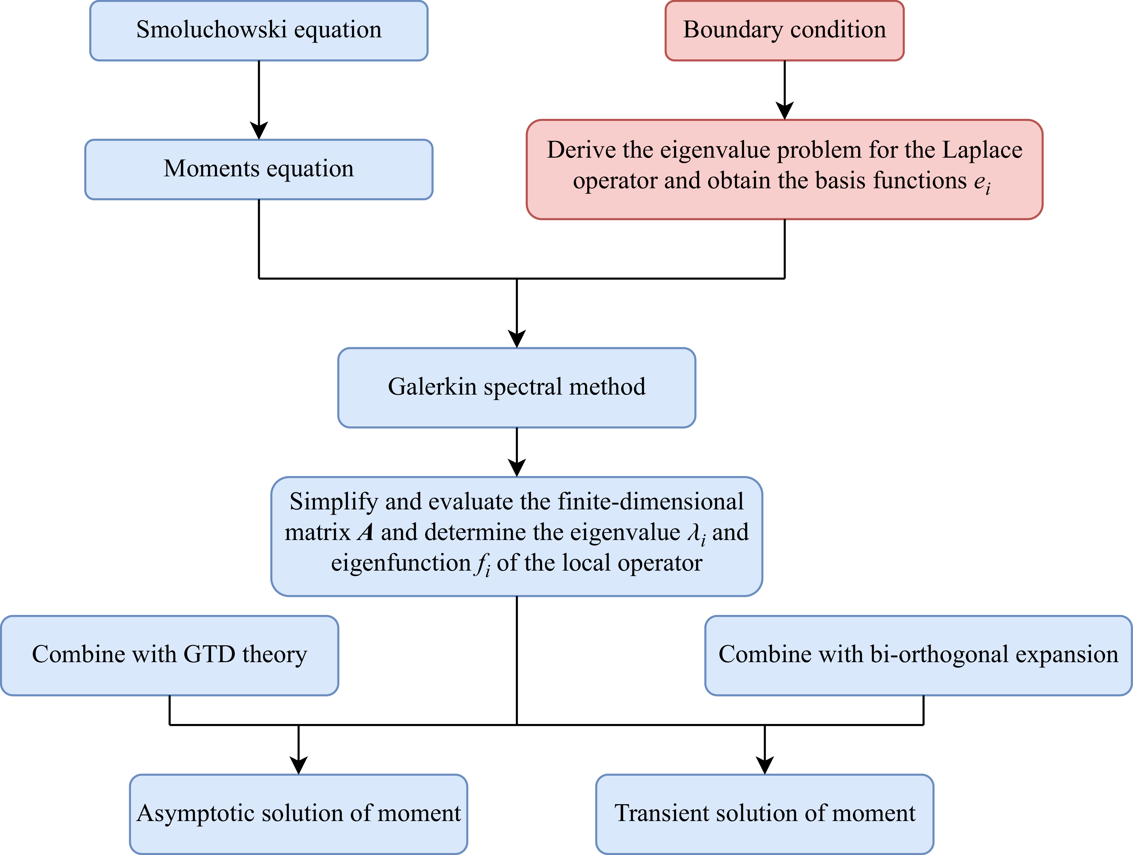
Flowchart of the solution procedure.

A flowchart of the solution procedure is presented in figure 2. To ensure convergence while keeping the computational cost at a reasonable level, in most cases we truncate the expansion series associated with the local space as follows: the maximum order in the radial direction is set to
 $n=120$
, and the highest degree of spherical harmonics in the swimming-direction space is taken as
 $l=12$
. For the transient problem, the bi-orthogonal expansion is further truncated at
 $N=40$
(where
 $N$
represents the total number of eigenfunctions used in the expansion (A1)).
4. Results of distribution
Many previous studies on microswimmers in pipe flows have focused on relatively small
 $\textit{Pe}_s$
. On the one hand, due to the limitations of classical models and their underlying assumptions, the analysis typically requires wall effects to be neglected and
 $\textit{Pe}_s$
to remain small. On the other hand, transport experiments with classical microorganisms such as microalgae in pipes usually employ millimetre- to centimetre-scale diameters and involve relatively limited swimming speeds (Croze et al. Reference Croze, Bearon and Bees2017), so the corresponding
 $\textit{Pe}_s$
is often not large. By contrast, our analytical framework does not impose an intrinsic restriction on
 $\textit{Pe}_s$
and mainly considers larger-
 $\textit{Pe}_s$
regimes (
 $\textit{Pe}_s\geqslant 10$
). Such regimes have been less explored in previous studies; here, swimming can markedly enhance cross-stream migration and increase the frequency of wall interactions, making the influence of boundary conditions on the distribution and dispersion more pronounced. In fact, large
 $\textit{Pe}_s$
is entirely feasible in experiments and applications. For example, glass capillaries commonly used in microfluidic systems can have radii as small as
 $R^*\approx 25$
μm, which is still much larger than the typical bacterial body length. Moreover, for artificial active particles and microrobots the propulsion speed can be tuned and can reach a few millimetres per second or even higher, for body lengths of a few tens of micrometres. For example, acoustically powered microrobots with a characteristic size of about
 $24$
μm have been reported to reach propulsion speeds up to
 $\sim 2.3\, \mathrm{mm} \,\mathrm{s}^{-1}$
(Aghakhani et al. Reference Aghakhani, Yasa, Wrede and Sitti2020); likewise, bioresorbable acoustic hydrogel microrobots with an outer diameter of about
 $30$
μm can achieve propulsion speeds of
 $2043\pm 280$
μm
 $\textrm{s}^{-1}$
in phosphate-buffered saline (Han et al. Reference Han2024). Under such micrometre-scale radii or elevated propulsion speeds, taking typical rotational diffusivities in the range
 $D_r^*\sim 0.05$
 $\mathrm{s}^{-1}$
readily gives
 $\textit{Pe}_s=\mathcal O(10)$
or even larger.
4.1. Local distribution
The local distribution
 $P_0^\infty$
represents the long-time asymptotic state of microswimmers in the zero-order moment space, corresponding to the steady-state probability density in the local domain
 $(r,\theta ,\phi )$
. We first compare the local distribution
 $P_0^\infty$
of ellipsoidal microswimmers under the diffuse-reflection boundary conditions and specular-reflection boundary conditions. For the previous specular-reflection boundary conditions (Jiang & Chen Reference Jiang and Chen2020; Guan et al. Reference Guan, Jiang, Wang, Zeng, Li and Chen2023), boundary conditions (2.12) and (2.14) become
 \begin{equation} P(r, \psi , z, \theta , \phi , t) = P(r, \psi , z, \theta , -\phi , t) \quad \mathrm{at} \quad r = 1, \end{equation}
 \begin{equation} \frac {\partial P}{\partial r}(r, \psi , z, \theta , \phi , t) = -\frac {\partial P}{\partial r}(r, \psi , z, \theta , -\phi , t) \quad \mathrm{at} \quad r = 1. \end{equation}
Local distribution
 $P_0^\infty$
of non-gyrotactic ellipsoidal microswimmers with different radial positions and boundary conditions. (a,c,e) Diffuse-reflection boundary conditions; (b,d, f) specular-reflection boundary conditions: (a,b)
 $r=0$
; (c,d)
 $r=0.5$
; (e, f)
 $r=0.99$
. Common parameters:
 $\textit{Pe}_s=10$
,
 $\textit{Pe}_{\!f}=10$
,
 $D_t=0.001$
,
 $\alpha _0=0.9$
,
 $\lambda =0$
.

Under the condition
 $\textit{Pe}_s = \textit{Pe}_{\!f} = 10$
(swimming speed comparable to the mean flow), microswimmers near the wall at
 $r=0.99$
preferentially align around
 $\theta =\pi /2$
and
 $\phi =0$
(upstream). With specular reflection, the distribution collapses tightly around
 $\phi =0$
, whereas with diffuse reflection the peak shifts into the sector
 $\phi \in (3\pi /2,\,2\pi )$
. This contrast indicates that diffuse reflection is a more effective reflection mechanism for driving microswimmers away from the wall and promoting cross-streamline migration, whereas specular reflection tends to favour high-shear trapping near the periphery. In figure 3(e), the distribution is nearly uniform over much of the domain because diffuse reflections randomise orientations. In figure 3( f), a clear symmetry appears, consistent with the mechanism of specular reflection.
At
 $r=0.5$
(mid-radius), microswimmers congregate near
 $\theta =\pi /2$
,
 $\phi =\pi$
(downstream) under both boundary conditions, but the clustering is markedly stronger with diffuse reflection. This further supports that diffuse scattering enhances cross-stream transport, drawing more swimmers from the wall towards the pipe centre. It also indicates that diffuse reflection substantially strengthens downstream alignment, so that in most of the interior region away from the boundary swimmers tend to migrate preferentially in the downstream direction. At
 $r=0$
(centreline), microswimmers again favour
 $\theta =\pi /2$
,
 $\phi =\pi$
, which indicates that their orientations are predominantly aligned with the downstream flow direction. Under diffuse reflection the orientation distribution is more anisotropic overall, with secondary accumulations also visible at
 $\theta =\pi /2$
,
 $\phi =\pi /2$
and
 $3\pi /2$
. All these results indicate that, compared with specular reflection, diffuse reflection enhances the cross-stream migration of microswimmers and amplifies the anisotropy of their orientations.
4.2. Asymptotic radial distribution
4.2.1. Influence of swimming and shear flow
Asymptotic radial distribution
 $C_r$
of non-gyrotactic ellipsoidal microswimmers with different swimming velocity and shear flow strength. The different parameters: (a)
 $\textit{Pe}_{\!f} =1$
; (b)
 $\textit{Pe}_{\!f} =5$
; (c)
 $\textit{Pe}_{\!f} =10$
; (d)
 $\textit{Pe}_{\!f} =20$
; (e)
 $\textit{Pe}_{\!f} =50$
; ( f)
 $\textit{Pe}_{\!f} =100$
. Common parameters:
 $D_t=0.001$
,
 $\alpha _0=0.9$
,
 $\lambda =0$
.

We next examine how the asymptotic radial concentration
 $C_r$
of non-gyrotactic ellipsoidal microswimmers changes with the swimming Péclet number
 $\textit{Pe}_s$
(swimming ability) and the shear Péclet number
 $\textit{Pe}_{\!f}$
(shear strength) (see figure 4). A notable feature across panels is that, whenever accumulation occurs in the high-shear region near
 $r=1$
, the concentration maximum is slightly off the wall rather than exactly at
 $r=1$
. This follows directly from diffuse reflection: upon wall contact, swimmers are randomly reoriented and are therefore efficiently returned into the interior instead of sticking to the boundary.
When
 $\textit{Pe}_s$
is small relative to
 $\textit{Pe}_{\!f}$
(e.g.
 $\textit{Pe}_s=0.1$
), cross-stream migration is weak; translational diffusion then levels the profile and
 $C_r$
is nearly uniform. Increasing
 $\textit{Pe}_s$
strengthens self-propulsion and the role of diffuse reflections, and swimmers accumulate more clearly in the high-shear near-wall region with the peak displaced slightly inward from the boundary. An interesting inversion appears when
 $\textit{Pe}_s$
becomes large compared with
 $\textit{Pe}_{\!f}$
: microswimmers migrate towards the pipe centre and the profile becomes monotonically decreasing from the centre to the wall. Unlike the conventional centre focusing produced by gyrotaxis (Croze et al. Reference Croze, Bearon and Bees2017; Jiang & Chen Reference Jiang and Chen2020), this centre-biased distribution here arises even without gyrotaxis. Diffuse reflection in a pipe provides an effective asymmetric transport mechanism that drives microswimmers from the wall region towards the centre, a feature that has not been reported under previously adopted specular-reflection boundary conditions. If
 $\textit{Pe}_s$
is made far larger still, the distribution tends back towards a more uniform state, because excessively strong cross-stream migration suppresses sustained local accumulation.
Varying
 $\textit{Pe}_{\!f}$
at fixed
 $\textit{Pe}_s$
further shows the influence of shear. As
 $\textit{Pe}_{\!f}$
increases, the radial profiles are progressively shaped by shear-induced alignment. For small
 $\textit{Pe}_s$
(0.1–1), the distribution evolves from nearly uniform to showing near-wall accumulation and then relaxes towards a more uniform state again. For moderate
 $\textit{Pe}_s$
(5–10), near-wall accumulation strengthens rapidly and the peak shifts closer to the boundary. For larger
 $\textit{Pe}_s$
(20–50), the profile transitions from almost uniform to pronounced centre focusing and ultimately to strong near-wall accumulation. In short, both very weak and very strong shear can yield nearly uniform profiles; intermediate shear may produce centre focusing; and stronger shear tends to produce the most intense near-wall accumulation.
From the dimensionless parameters (2.3), when the influence of translational diffusion is small, proportionally increasing
 $\textit{Pe}_s$
and
 $\textit{Pe}_{\!f}$
is effectively equivalent to strengthening the role of rotational reorientation (since both numbers scale together). Comparing the five cases
 $\textit{Pe}_s=\textit{Pe}_{\!f}=1,\,5,\,10,\,20,\,50$
, one observes that, as the rotational diffusion increases, near-wall accumulation first intensifies and then weakens; correspondingly, the location of the maximum shifts from near the wall to at the wall and then drifts back towards the interior.
4.2.2. Influence of gyrotaxis and flow direction
Asymptotic radial distribution
 $C_r$
of ellipsoidal microswimmers with different gyrataxis and flow direction. The different conditions: (a,c)
 $\textit{Pe}_{\!f}=10$
; (b,d)
 $\textit{Pe}_{\!f}=100$
; (a,b) flow direction is vertically downward; (c,d) flow direction is vertically upward. Here, ‘specular’ denotes the results obtained under the specular-reflection boundary condition. Common parameters:
 $\alpha _0=0.9$
,
 $\textit{Pe}_s=20$
,
 $D_t=0.001$
.

Figure 5 shows the radial distributions of ellipsoidal microswimmers with different gyrotactic strengths and flow directions. For non-gyrotactic microswimmers, reversing the flow direction does not affect the radial distribution; unless otherwise stated, we henceforth consider the downwelling flow throughout the paper. When the swimming ability is much stronger than the shear (
 $\textit{Pe}_s \gg \textit{Pe}_{\!f}$
), the effect of gyrotaxis on the radial distribution is relatively small. An interesting feature emerges in figure 5(a,c): under diffuse-reflection boundary conditions, in vertically downward flow, gyrotactic microswimmers accumulate near the pipe wall, whereas in vertically upward flow they gather in the central region of the pipe. This is opposite to the classical phenomenon of gyrotactic focusing in pipes (Kessler Reference Kessler1985, Reference Kessler1986; Croze et al. Reference Croze, Bearon and Bees2017), and such behaviour is not observed under the previously studied specular-reflection condition, for which the distribution remains consistent with the classical results. In this regime, swimming and boundary scattering dominate the migration. Microswimmers collide frequently with the wall, and each collision is followed by diffuse reflection that randomises their orientation, which suppresses the focusing produced by gyrotactic reorientation. As gyrotaxis is strengthened, it effectively acts like a reduction in swimming strength, so shear becomes comparatively more influential. In downward flow this favours trapping in the high-shear near-wall region. In upward flow the observed centre accumulation arises from diffuse reflection: although the combined action of gyrotaxis and shear tends to bias microswimmers towards the wall, their near-wall orientations are not fully aligned with the streamwise direction and retain substantial normal components because of gyrotaxis. These normal components increase the impact of diffuse reflections, promoting migration away from the boundary and towards the pipe centre. In fact, due to the complexity of the real motion and near-wall behaviours of natural microorganisms, as well as the challenges and limitations in experimental observations, it is difficult at present to make quantitative comparisons between theoretical and experimental results, and one can usually only attempt qualitative comparisons. In the future, for artificial particles and microrobots, it may be possible to employ suitable boundary designs and active control strategies, for instance by providing sufficiently strong self-propulsion and engineering a diffuse-reflection-type response upon wall encounters, so that these specific distribution and migration phenomena can be realised.
Some of the steeper curves exhibit some fluctuations near
 $r=0$
. This may be due to the fact that the Poiseuille shear vanishes at the pipe centre, so shear-induced reorientation is weakest there; as a result, microswimmers can migrate more freely towards different directions, leading to a small local dip or peak in
 $C_r$
, similar to what can occur near the channel centre in planar Poiseuille flows. Increasing the number of basis functions can make this feature smoother. Moreover, it can be seen that, when
 $\lambda =2$
(figure 5
a), the swimmers exhibit an almost uniform radial distribution. This reflects a delicate balance among the boundary condition, gyrotaxis and shear-induced alignment. However, this balance is fragile: stronger shear cannot fully counteract gyrotaxis to maintain such uniformity, and it tends to break down under higher shear. When
 $\textit{Pe}_{\!f}$
is significantly larger than
 $\textit{Pe}_s$
, the radial distributions exhibit the classical gyrotactic patterns. For downward flows, gyrotaxis leads to accumulation at the centre; for upward flows, it drives accumulation near the pipe wall. In this case, the influence of the boundary condition is relatively weak, and the distribution trends of gyrotactic microswimmers are similar under the two boundary conditions. As gyrotaxis becomes stronger, the resulting accumulation becomes more pronounced. The influence of shear is also evident. Compared with the weak-shear case, as the shear strength increases the radial distribution trend completely reverses, because shear largely weakens the effects of swimming and boundary interactions, leaving shear and gyrotaxis to dominate the migration. Moreover, the gyrotactic focusing is stronger in upwelling flows than in downwelling flows, because in the latter high-shear trapping and gyrotaxis act in concert, whereas in the former they compete.
4.2.3. Influence of shape
Asymptotic radial distribution
 $C_r$
of microswimmers with different shapes in downwelling flow. The different parameters: (a)
 $\lambda =0$
,
 $\textit{Pe}_{\!f}=10$
; (b)
 $\lambda =0$
,
 $\textit{Pe}_{\!f}=50$
; (c)
 $\lambda =2$
,
 $\textit{Pe}_{\!f}=10$
; (d)
 $\lambda =2$
,
 $\textit{Pe}_{\!f}=50$
. Common parameters:
 $D_t=0.001$
,
 $\textit{Pe}_s=10$
.

Figure 6 shows the radial distributions of microswimmers with different shapes in downwelling flow. For non-gyrotactic spherical microswimmers, the diffuse-reflection boundary condition yields a perfectly uniform radial distribution. In fact, the corresponding local distribution admits a constant solution
 $P_0^{\infty }= {1}/{4\pi }$
, identical to the result under specular reflection (Jiang & Chen Reference Jiang and Chen2019). Under moderate shear (
 $\textit{Pe}_{\!f}=10$
), increasing the shape factor
 $\alpha _0$
first makes the radial profile more non-uniform and then gradually more uniform again. Ellipsoidal shapes enhance shear alignment, which initially promotes accumulation in the high-shear near-wall region; however, when the swimmers become sufficiently slender, the strong near-wall accumulation is offset by diffuse reflections that redirect swimmers back towards the centre, thereby weakening the wall accumulation.
A similar pattern appears under stronger shear, but the
 $\alpha _0$
threshold at which the trend reverses shifts to larger values. Strong shear reduces cross-stream migration and diminishes the influence of the boundary, so near-wall swimmers find it harder to move from the wall towards the centre. In figure 6(c,d), where gyrotaxis is present, increasing
 $\alpha _0$
drives a clear transition from centreline focusing to near-wall accumulation. This indicates that shear alignment induced by elongation counteracts and eventually suppresses the gyrotactic focusing at the centre. The coupling among shear, gyrotaxis and the boundary condition produces richer migration dynamics and distribution patterns.
4.2.4. Influence of translational diffusion
Asymptotic radial distribution
 $C_r$
of ellipsoidal microswimmers with different translational diffusion. The different parameters: (a)
 $\lambda =0$
,
 $\textit{Pe}_{\!f}=10$
; (b)
 $\lambda =0$
,
 $\textit{Pe}_{\!f}=100$
; (c)
 $\lambda =2$
,
 $\textit{Pe}_{\!f}=10$
; (d)
 $\lambda =2$
,
 $\textit{Pe}_{\!f}=100$
. Common parameters:
 $\alpha _0=0.9$
,
 $\textit{Pe}_s=1$
.

In figure 7, we explore the influence of translational diffusion on the radial distribution of ellipsoidal microswimmers. Under non-gyrotactic conditions (
 $\lambda =0$
), translational diffusion competes directly with the microswimmers’ cross-stream migration. When
 $\textit{Pe}_s/\textit{Pe}_{\!f}$
is smaller (i.e. strong shear relative to swimming), ellipsoids align more with the flow and their cross-stream migration weakens, so the competing action of translational diffusion becomes more prominent. This is reflected in figure 7(a,b): at
 $\textit{Pe}_{\!f}=10$
, reducing
 $D_t$
transforms
 $C_r$
from nearly uniform to clearly wall-increasing, with centreline depletion emerging; at
 $\textit{Pe}_{\!f}=100$
, the trend strengthens – profiles become monotonically increasing in
 $r$
, and only a large
 $D_t$
(
 $10^{-1}$
) can appreciably homogenise the distribution. This is reflected in figure 7(a,b): at
 $\textit{Pe}_{\!f}=10$
, reducing
 $D_t$
leads to increasingly strong near-wall accumulation, with little further change once
 $D_t\leqslant 10^{-3}$
; at
 $\textit{Pe}_{\!f}=100$
, the distribution keeps becoming more non-uniform for all
 $D_t$
, and the overall trend grows stronger as
 $D_t$
decreases.
With gyrotaxis (
 $\lambda =2$
), the balance shifts: gyrotactic reorientation enhances cross-stream migration towards the centre, while translational diffusion counteracts that accumulation. Figure 7(c,d) shows that decreasing
 $D_t$
raises the concentration near the centre region and deepens the decay towards the wall. Moreover, comparing figures 7(a) and 7(c) as well as figures 7(b) and 7(d), it can be found that the influence of translational diffusion is stronger in the presence of gyrotaxis, indicating that gyrotaxis-induced cross-stream migration is also relatively weak. Overall, the smaller the ratio
 $\textit{Pe}_s/\textit{Pe}_{\!f}$
, the weaker the ellipsoids’ cross-stream migration and the stronger the relative impact of translational diffusion, which tends to homogenise the spatial distribution and suppress local accumulation effects, including those induced by shear or gyrotaxis.
4.3. Transient radial distribution
Transient radial distribution
 $C_t$
of microswimmers at different times. The different parameters: (a)
 $t=0.05$
; (b)
 $t=0.1$
; (c)
 $t=0.2$
; (d)
 $t=0.5$
. The case ‘Gyrotactic spherical’ corresponds to
 $\lambda = 2, \alpha _0 = 0$
; ‘Non-gyrotactic ellipsoidal’ corresponds to
 $\lambda = 0, \alpha _0 = 0.9$
; ‘Gyrotactic ellipsoidal’ corresponds to
 $\lambda = 2,{} \alpha _0 = 0.9$
; and ‘Gyrotactic ellipsoidal, specular’ corresponds to
 $\lambda = 2, \alpha _0 = 0.9$
with specular-reflection boundary conditions. Common parameters:
 $D_t=0.001,\ \textit{Pe}_s=10,\ \textit{Pe}_{\!f}=10$
.

The transient radial distributions at different times are shown in figure 8. At the earliest time (
 $t=0.05$
), the four cases exhibit significant distinctions. The gyrotactic spherical microswimmers are nearly uniform, with only slight accumulation at the pipe centre. In contrast, both the gyrotactic and the non-gyrotactic ellipsoidal microswimmers display an M-shaped radial pattern: low concentration at the pipe centre and near the wall, with two local maxima around
 $r\approx 0.3$
and
 $r\approx 0.75$
. For the gyrotactic ellipsoidal microswimmers with specular reflection, the distribution is different – distribution is relatively high near
 $r\approx 0.6$
and at the wall. These features indicate that, at early times, shear-induced alignment and the boundary condition exert the dominant influence, with diffuse reflection enabling faster and more efficient escape from the wall. At
 $t=0.1$
, a clear centreline accumulation has already emerged for the gyrotactic spherical microswimmers, with
 $C_t$
decreasing from the centre to the wall. The other three ellipsoidal microswimmer cases all evolve into near-wall accumulation, and under specular reflection the microswimmer concentration is higher across most of the interior region (
 $r \approx 0.2$
to
 $r \approx 0.6$
). At this stage, gyrotactic effects begin to take hold, shear effects further dominate and under specular reflection the higher concentration in the interior region results from migration caused by wall reflections at
 $t=0$
.
By
 $t=0.2$
, the transient radial distributions of the gyrotactic and non-gyrotactic ellipsoidal swimmers are nearly identical, indicating that strong swimming and shear alignment can substantially suppress gyrotactic effects at this stage. These tendencies strengthen: centre accumulation grows steadily for the gyrotactic spherical microswimmers, whereas the other three ellipsoidal cases develop stronger near-wall accumulation, and under specular reflection the microswimmer concentration is higher over most of the central region (
 $r \leqslant 0.5$
). From
 $t=0.2$
to
 $t=0.5$
, the centreline focusing of gyrotactic spherical microswimmers intensifies further. By contrast, the near-wall accumulation of both gyrotactic and non-gyrotactic ellipsoidal microswimmers weakens while the central concentration increases, because swimming and diffuse reflections remain sufficiently strong in this stage to help a fraction of swimmers escape high-shear trapping near the wall. Moreover, the specular-reflection case shows the smallest subsequent change in its transient radial profile, implying the shortest relaxation time to the asymptotic regime; this is because of weaker cross-stream migration under specular reflection, which favours trapping in high-shear regions. In contrast, the gyrotactic spherical swimmers display the longest relaxation time. Except for the spherical microswimmers, whose transient radial distribution varies monotonically with time, the other three cases exhibit non-monotonic evolution. This behaviour mainly results from the competition between boundary effects and shear alignment: boundary effects dominate at the initial stage, whereas shear effects take over at later times.
5. Results of dispersion coefficients
5.1. Asymptotic drift velocity and dispersivity
Drift velocity
 $U^{\infty }_d$
and dispersivity
 $D^{\infty }_T$
of microswimmers as functions of
 $\textit{Pe}_s$
or
 $\textit{Pe}_{\!f}$
: (a,b) as functions of
 $\textit{Pe}_s$
,
 $\textit{Pe}_{\!f}=10$
; (c,d) as functions of
 $\textit{Pe}_{\!f}$
,
 $\textit{Pe}_s=10$
. The case ‘Gyrotactic spherical’ corresponds to
 $\lambda = 2, \alpha _0 = 0$
; ‘Non-gyrotactic ellipsoidal’ corresponds to
 $\lambda = 0, \alpha _0 = 0.9$
; ‘Gyrotactic ellipsoidal’ corresponds to
 $\lambda = 2, \alpha _0 = 0.9$
; and ‘Gyrotactic ellipsoidal, specular’ corresponds to
 $\lambda = 2,{} \alpha _0 = 0.9$
with specular-reflection boundary conditions. Common parameters:
 $D_t=0.001$
.

As shown in figure 9, we explore the drift velocity
 $U_d^\infty$
and dispersivity
 $D_T^\infty$
of microswimmers as a function of
 $\textit{Pe}_s$
or
 $\textit{Pe}_{\!f}$
. The drift velocity represents the mean streamwise migration of the suspension relative to the mean flow; an individual microswimmer’s velocity combines the background advection with its self-propulsion. In figure 9(a), the gyrotactic spherical microswimmers show a monotonic decrease of
 $U_d^\infty$
with increasing
 $\textit{Pe}_s$
. Gyrotaxis drives swimmers to accumulate around the pipe centre (where the Poiseuille flow velocity is largest), whereas stronger swimming counteracts this gyrotactic bias and gradually weakens centreline accumulation, thus reducing the drift. For non-gyrotactic ellipsoidal microswimmers,
 $U_d^\infty$
first increases and then decreases. This can be interpreted from the local/orientational and radial distributions: as swimming strengthens, the preferred accumulation shifts from the near-wall region towards the centre, which initially increases the drift; later, orientations become more dispersed, which later reduces the net streamwise propulsion and diminishes the drift. For gyrotactic ellipsoidal microswimmers,
 $U_d^\infty$
decreases at first and then increases. This trend is opposite to that of non-gyrotactic ellipsoids because moderate swimming initially weakens the gyrotaxis-induced centre aggregation (reducing the drift), whereas sufficiently strong swimming subsequently promotes centre accumulation again (increasing the drift). Under specular reflection, gyrotactic ellipsoids exhibit a persistently decreasing
 $U_d^\infty$
: at small
 $\textit{Pe}_s$
the dynamics is governed by shear and gyrotaxis, so boundary effects are relatively weak and the results are close to those under diffuse reflection; indeed, in this strong-shear regime Croze et al. (Reference Croze, Bearon and Bees2017) employed classical models for spherical gyrotactic swimmers and obtained good agreement with experiments. At larger
 $\textit{Pe}_s$
, wall effects become stronger and specular reflections are less able than diffuse reflections to redirect swimmers to the centre, which further suppresses the drift.
Figure 9(c) shows how the shear flow strength modulates the drift. For non-gyrotactic ellipsoidal microswimmers, when
 $\textit{Pe}_{\!f}$
is small the ratio
 $\textit{Pe}_s/\textit{Pe}_{\!f}$
is large, the radial and orientation distribution is relatively uniform and
 $U_d^\infty$
is near zero. As
 $\textit{Pe}_{\!f}$
increases,
 $\textit{Pe}_s/\textit{Pe}_{\!f}$
decreases yet swimming still dominates; microswimmers shift slightly towards the centre as the background speed rises, and their swimming directions in most of the central region tend to align with the streamwise flow, so the drift increases. When
 $\textit{Pe}_{\!f}$
becomes sufficiently large, shear dominates, ellipsoidal microswimmers accumulate near the wall and their swimming directions tend to align with the negative streamwise direction, leading to a decline in drift. The other three cases exhibit the opposite overall trend to figure 9(a). Gyrotactic spherical microswimmers exhibit an initial decrease in
 $U_d^\infty$
because shear first promotes near-wall accumulation; as shear increases further, it weakens the self-propulsion competing with gyrotaxis, allowing gyrotactic focusing to strengthen and leading to a subsequent rise in
 $U_d^\infty$
, which is consistent with the drift velocity trends reported in previous studies in the small-
 $\textit{Pe}_s$
regime (Croze et al. Reference Croze, Bearon and Bees2017; Jiang & Chen Reference Jiang and Chen2020). Gyrotactic ellipsoidal microswimmers with diffuse reflection exhibit a trend similar to that of non-gyrotactic ellipsoidal microswimmers, but with a smaller drift velocity, because gyrotaxis weakens the swimming ability and makes the swimmers more prone to migrate into high-shear regions. Under specular reflection, gyrotactic ellipsoids remain weakly sensitive to
 $\textit{Pe}_{\!f}$
and keep a comparatively small (often negative) drift, as specular impacts favour persistent near-wall residence and limit recovery of centreline accumulation even when the mean flow intensifies.
Dispersivity characterises how microswimmers spread within the fluid, and the overall dispersion process comprises both swimming-induced diffusion and convective dispersion. As
 $\textit{Pe}_s$
increases in figure 9(b), three cases – gyrotactic spherical microswimmers, gyrotactic ellipsoidal microswimmers with diffuse reflection and gyrotactic ellipsoidal microswimmers with specular reflection – show
 $D_T^{\infty }$
that first increases, then decreases and finally increases again. At small
 $\textit{Pe}_s$
, dispersion is dominated by convective effects, as stronger swimming amplifies concentration non-uniformity and boosts convective dispersion; at intermediate
 $\textit{Pe}_s$
, swimming competes with gyrotaxis and reduces centreline accumulation, weakening the convective part; at large
 $\textit{Pe}_s$
, the swimming-induced contribution dominates and
 $D_T^{\infty }$
rises once more. The non-gyrotactic ellipsoidal microswimmers are different:
 $D_T^\infty$
increases and then only slightly decreases, because the enhanced swimming ability first promotes convection and later weakens it. For gyrotactic ellipsoidal microswimmers, at
 $\textit{Pe}_s\lt 4$
the dispersivity under diffuse reflection is slightly larger than that under specular reflection because convective dispersion is stronger; beyond that, the specular case becomes larger because diffuse reflections more effectively randomise orientations and thus weaken the swimming-induced dispersion effect at high
 $\textit{Pe}_s$
. Overall, both gyrotaxis and ellipsoidal shape can increase dispersivity, whereas diffuse-reflection boundary conditions can reduce it at large
 $\textit{Pe}_s$
.
Varying
 $\textit{Pe}_{\!f}$
reveals distinct dispersion regimes across swimmer types and boundary conditions. As
 $\textit{Pe}_{\!f}$
increases, the dispersivity of gyrotactic ellipsoidal microswimmers with specular reflection rises monotonically and remains the largest among the cases. For gyrotactic ellipsoids with diffuse reflection, dispersivity first increases and then decreases, yet it stays above that of non-gyrotactic ellipsoids throughout. These trends further indicate that diffuse reflection can reduce dispersivity at large
 $\textit{Pe}_s$
, whereas gyrotaxis can enhance it. In addition, gyrotactic spherical microswimmers display a non-monotonic ‘increase–decrease–increase’ response with
 $\textit{Pe}_{\!f}$
: at small
 $\textit{Pe}_{\!f}$
, shear strengthens gyrotactic focusing and thereby boosts convective dispersion; at intermediate
 $\textit{Pe}_{\!f}$
, the swimming-induced diffusional contribution is weakened; at large
 $\textit{Pe}_{\!f}$
, convection is again promoted, leading to a renewed rise in dispersivity.
5.2. Transient drift velocity and dispersivity
Transient drift velocity and dispersivity of microswimmers: (a,b)
 $\textit{Pe}_s=1$
; (c,d)
 $\textit{Pe}_s=10$
. The case ‘Gyrotactic spherical’ corresponds to
 $\lambda = 2, \alpha _0 = 0$
; ‘Non-gyrotactic ellipsoidal’ corresponds to
 $\lambda = 0,{} \alpha _0 = 0.9$
; ‘Gyrotactic ellipsoidal’ corresponds to
 $\lambda = 2, \alpha _0 = 0.9$
; and ‘Gyrotactic ellipsoidal, specular’ corresponds to
 $\lambda = 2, \alpha _0 = 0.9$
with specular-reflection boundary conditions. Common parameters:
 $\textit{Pe}_{\!f}=10,{} D_t=0.001$
.

Figure 10 shows the transient drift velocity and dispersivity of microswimmers at different time instants. With a spatially uniform release, the initial drift velocity is essentially zero in all cases. Under strong-shear conditions, the transient drift velocity of microswimmers in all four cases varies monotonically with time. The gyrotactic spherical microswimmers develop an ever larger positive drift, and gyrotactic ellipsoidal microswimmers also increase but to a more moderate level. By contrast, non-gyrotactic ellipsoidal microswimmers exhibit a steadily decreasing drift that becomes negative. The gyrotactic ellipsoids with specular reflection follow the same qualitative growth as the diffuse-reflection case and remain close to it throughout. These behaviours reflect, under strong shear, the roles of gyrotaxis and shape-induced shear alignment: gyrotaxis drives microswimmers towards the pipe centre, thereby increasing the transient drift velocity; meanwhile, ellipsoidal shape strengthens shear alignment, so swimmers near the wall tend to orient in the negative streamwise direction, which reduces the transient drift velocity. Because shear dominates when
 $\textit{Pe}_s$
is small, the boundary condition has only a minor impact on the drift velocity.
All four cases show transient dispersivity that first increases with time and then decreases towards an asymptotic value. For
 $t\lt 2$
, the behaviours are nearly identical, but they gradually diverge thereafter: the non-gyrotactic ellipsoidal microswimmers always attain the largest dispersivity, the gyrotactic ellipsoidal microswimmers lie in between and the gyrotactic spherical microswimmers display the smallest dispersivity, which eventually decays to a very low value. The early dispersion is dominated by convection, with migration controlled by shear-induced rotation. For gyrotactic spherical microswimmers, the progressive buildup of centreline accumulation weakens convective dispersion, leading to a continual decline of dispersivity to a low level. For gyrotactic ellipsoidal microswimmers, shear alignment counteracts centreline focusing and drives part of the population towards the wall, so their dispersivity decreases later but remains larger than that of gyrotactic spherical microswimmers. For non-gyrotactic ellipsoidal microswimmers, the radial distribution remains comparatively uniform, with substantial populations both at the wall and in the centre, resulting in the strongest convection and the highest transient dispersivity.
When swimming is strong, the transient drift of non-gyrotactic ellipsoidal and gyrotactic ellipsoidal microswimmers follows a ‘rise–fall–rise’ pattern, with the non-gyrotactic ellipsoidal microswimmers maintaining the largest drift throughout. This sequence is consistent with the transient radial distributions: diffuse reflection first drives swimmers away from the wall and into the interior, so the background Poiseuille flow boosts the drift; subsequently, shear-induced alignment pushes swimmers back towards the wall, reducing the background-driven contribution and lowering the drift; later, wall accumulation weakens, orientations near the centre tend to align downstream and both the background flow and self-propulsion raise the drift again. Gyrotaxis further weakens effective swimming and strengthens near-wall trapping, so the gyrotactic ellipsoids remain below the non-gyrotactic ones. By contrast, gyrotactic spherical microswimmers and gyrotactic ellipsoidal microswimmers with specular-reflection conditions show a monotonic decline of transient drift. In the specular case, shear consistently dominates the migration: swimmers slide and accumulate near the wall, and the drift decreases steadily. For gyrotactic spheres, gyrotaxis suppresses downstream swimming and promotes centre focusing that reduces exposure to high-speed regions, so the drift likewise decays with time. Except for gyrotactic spherical microswimmers, the other three cases exhibit transient dispersivity that first increases and then decreases, similar to the behaviour under strong shear with small
 $\textit{Pe}_s$
. For gyrotactic spherical microswimmers, strong swimming weakens gyrotactic effects, and shear-induced rotation promotes a more uniform orientation, so the time evolution of transient dispersivity is more fluctuating.
6. Concluding remarks
Because of the high dimensionality and geometric complexity of the circular-pipe problem, formulating and implementing boundary conditions are challenging, and most existing theoretical studies either neglect boundary effects or impose purely specular-reflection boundary conditions. To address this gap, an analytical model is devised and explored for microswimmer dispersion in a cylindrical-pipe flow under diffuse-reflection boundary conditions, extending our earlier studies (Jiang & Chen Reference Jiang and Chen2020; Zeng et al. Reference Zeng, Jiang, Guan, Lee and Chen2025b
). We propose an appropriate mathematical formulation of the diffuse-reflection boundary condition in a continuum model for a cylindrical pipe, so as to ensure that the associated Laplacian eigenvalue problem is well posed. We then analytically derive the corresponding Laplacian eigenvalue problem and obtain a complete set of basis functions given by products of Bessel functions and spherical harmonics. The resulting moment equations are solved using a Galerkin spectral method, and the computation is simplified by decomposing the operator, exploiting the separable structure of the basis functions and evaluating the orientational integrals using Wigner
 $3j$
symbols. Many previous studies on microswimmers in pipe flows have focused on relatively small swimming Péclet numbers
 $\textit{Pe}_s$
, whereas this study mainly focuses on regimes with relatively large
 $\textit{Pe}_s$
, for which wall effects are pronounced and cannot be neglected. The study follows the entire transport process, examining the local distribution, the radial distribution, the drift velocity and the dispersivity, and investigates how key parameters affect these results, with comparisons with the specular-reflection boundary conditions.
Compared with specular reflection, diffuse reflection is a more efficient way to drive microswimmers away from the wall, and it promotes downstream orientation and cross-stream migration. When swimming is strong, a distinct phenomenon arises for non-gyrotactic spheroidal microswimmers: they accumulate in the central region of the pipe. In previous studies, such centreline accumulation is typically observed only for gyrotactic swimmers, and is not expected for non-gyrotactic ones. Moreover, gyrotaxis can lead to near-wall accumulation in downwelling flow. This effect can oppose diffuse reflection and produce an approximately uniform radial distribution. In upwelling flow, gyrotaxis instead promotes accumulation near the pipe centre. These behaviours are opposite to those of classical gyrotactic focusing and arise from the combined actions of diffuse reflection, gyrotaxis and shear alignment. In addition, when the shear is sufficiently strong relative to swimming, shear alignment can promote near-wall accumulation on its own, and it can also act together with gyrotaxis to produce classical gyrotactic focusing.
Increasing slenderness first strengthens and then weakens near-wall accumulation, and it also diminishes gyrotactic centreline focusing, with shape effects becoming even more pronounced under strong shear. Translational diffusion hinders cross-stream migration and promotes radial uniformity, with an influence that grows as
 $\textit{Pe}_s/\textit{Pe}_{\!f}$
decreases; under strong shear,
 $D_t$
suppresses both shear-induced wall trapping and gyrotaxis-induced centre focusing. When swimming is strong, ellipsoidal swimmers display distinctly different radial distribution patterns across different stages of the transient evolution, and under diffuse reflection an early-time M-shaped double-peaked profile emerges on both sides of the centreline. This behaviour reflects a shift in the dominant mechanism over time: boundary effects dominate initially, gyrotaxis dominates at later times and shear acts throughout the process. Diffuse reflection exhibits a shorter relaxation time and a stronger boundary effect than specular reflection.
For ellipsoidal microswimmers, the drift velocity varies non-monotonically with both
 $\textit{Pe}_s$
and
 $\textit{Pe}_{\!f}$
, whereas for gyrotactic ellipsoids under specular reflection it changes monotonically. This contrast mainly arises because, under diffuse reflection, microswimmers can develop distinctly different distribution patterns at relatively small and relatively large
 $\textit{Pe}_s$
. Both gyrotaxis and ellipsoidal shape can increase the dispersivity, and in most cases diffuse reflection yields a larger drift velocity and a smaller dispersivity than specular reflection. Under strong shear, the transient drift varies monotonically in time. Because convective dispersion dominates the early stage of the transport process, the transient dispersivity is initially similar across different cases and then typically increases before decreasing. Under strong swimming, ellipsoidal swimmers exhibit a rise–fall–rise transient drift in time, whereas spherical swimmers and ellipsoids under specular reflection show a continual decrease.
This study explores microswimmer dispersion in cylindrical pipes under a diffuse-reflection boundary condition. It helps fill the knowledge gap associated with boundary conditions in circular pipes and provides a foundation for future studies of more complex and refined wall models. It is also worth emphasising that our goal is not to model any specific natural microorganism. Rather, the framework is more suitable for controllable synthetic active particles and microrobots, for which propulsion and wall responses can be engineered, making the predicted distribution and migration phenomena easier to realise and manipulate. For instance, one may provide sufficiently strong self-propulsion and design a diffuse-reflection-type response upon wall encounters. Together, these results advance our understanding of the mechanisms that govern microswimmer transport and its control.
This study employs relatively simplified and idealised boundary conditions in the continuum model. Future work could propose more refined boundary conditions to capture more complex and realistic problems, for instance by prescribing a non-uniform distribution of scattering angles or by adopting mixed reflection laws in which specular and diffuse reflections coexist. A systematic comparison with individual-based simulations would also be valuable to validate the continuum description and delineate its limitations, including identifying the parameter regimes over which it remains accurate. In particular, microswimmers may exhibit residence behaviours such as tumbling (Bearon & Hazel Reference Bearon and Hazel2015; Ezhilan & Saintillan Reference Ezhilan and Saintillan2015; Zeng et al. Reference Zeng, Chen, Guo, Jiang and Chen2025a ) or sliding upon encountering walls, which have been observed in experiments with E. coli and Chlamydomonas. In addition, the present study is restricted to dilute suspensions and neglects swimmer–flow coupling (Hwang & Pedley Reference Hwang and Pedley2014b ), which can modify both dispersion and hydrodynamic instabilities. Future work should employ a more refined bidirectionally coupled model to account for this effect, thereby providing more comprehensive theoretical predictions. Besides, this study considers only gyrotaxis, whereas microswimmers can also exhibit behaviours such as chemotaxis (Bearon & Pedley Reference Bearon and Pedley2000) and magnetotaxis (Kumaran Reference Kumaran2021).
Acknowledgements
The authors thank W. Jiang and M. Guan for helpful discussions.
Funding
This work is supported by the National Natural Science Foundation of China (grant no. 12372379).
Declaration of interests
The authors report no conflict of interest.
Appendix A. Bi-orthogonal expansion method
For the transient solution of the zeroth-order moment (which depends on the time variable
 $t$
), we perform an eigenfunction expansion to separate the time variable
 $t$
from the spatial variables
 $(r,\theta ,\phi )$
:
 \begin{equation} \begin{aligned} P_0 = \sum _{i=1}^{\infty } p_{i} \mathrm{e}^{\lambda _i t} f_i(r,\theta ,\phi ) , \end{aligned} \end{equation}
with the eigenvalue problem of
 $\mathcal{L}$
,
 \begin{equation} \mathcal{L} f_i = \lambda _i f_i, \quad i =1,2,\ldots, \end{equation}
where
 $p_i$
are the expansion coefficients determined by the initial conditions,
 $\lambda _i$
are the eigenvalues arranged in descending order and
 $f_i$
are the corresponding eigenfunctions. Note that
 $\lambda _1 = 0$
, and the associated eigenfunction
 $f_1$
corresponds to a multiple of the asymptotic solution
 $P_0^{\infty }$
. Similarly, we employ the Galerkin spectral method to solve this eigenvalue problem. According to the definition of the bilinear form (3.40), the eigenvalue problem (A2) is transformed into a matrix problem:
 \begin{equation} \boldsymbol{A} \boldsymbol{\phi }_i = \lambda _i \boldsymbol{\phi }_i, \end{equation}
where
 $\boldsymbol{\phi _i}$
is the eigenvector corresponding to
 $\lambda _i$
, representing the column vector of expansion coefficients of
 $f_i$
with respect to the basis functions
 $\{e_i\}_{i=1}^\infty$
.
Because operator
 $\mathcal{L}$
is non-self-adjoint, the eigenfunctions
 $\{f_i\}_{i=1}^\infty$
are no longer orthogonal, and the expansion coefficients
 $p_i$
cannot be directly computed. The adjoint eigenfunctions
 $\{f_i^{\star }\}_{i=1}^\infty$
are introduced to resolve this issue. The two sets,
 $\{f_i\}_{i=1}^\infty$
and
 $\{f_i^{\star }\}_{i=1}^\infty$
, satisfy the bi-orthogonality relation
 \begin{equation} \langle f_i^{\star }, f_{\!j} \rangle = \delta _{\textit{ij}}, \end{equation}
where
 $\delta _{\textit{ij}}$
denotes the Kronecker delta symbol.
The adjoint eigenfunctions
 $\{f_i^{\star }\}_{i=1}^\infty$
are eigenfunctions of the adjoint operator
 $\mathcal{L}^{\star }$
. Hence, we again employ the Galerkin method to solve the eigenvalue problem of the adjoint operator. Let
 $A^{\star }$
denote the matrix associated with the adjoint operator. Then
 \begin{equation} \boldsymbol{A}^{\star }\boldsymbol{\phi }_i^{\star } = \lambda _i^{} \boldsymbol{\phi }_i^{\star }, \end{equation}
where
 $\boldsymbol{\phi }_i^{\star }$
represents the column vector of expansion coefficients of
 $f_i^{\star }$
with respect to the basis functions
 $\{e_i\}_{i=1}^\infty$
and
 $\boldsymbol{A}^{\star } = \boldsymbol{A}^{{T}}$
. We note that, besides the bilinear form adopted here, one may alternatively define the pairing by a complex inner product with conjugation in the first argument, and construct the corresponding bi-orthogonal basis (Ding & McLaughlin Reference Ding and McLaughlin2022; Jiménez-Urias & Haine Reference Jiménez-Urias and Haine2023; Ding Reference Ding2025). Under this convention, the adjoint eigenvalues become the complex conjugates of those in the original eigenproblem. In the Galerkin framework, this corresponds to the adjoint matrix
 $A^{\star }=A^{ H}$
(the conjugate transpose); since
 $A$
is real,
 $A^{H}=A^{T}$
, so the computed results are identical and only the notation for the adjoint problem differs.
After obtaining the adjoint eigenfunctions
 $\{f_i^{\star }\}_{i=1}^\infty$
, the expansion coefficients
 $\{p_{i}\}_{i=1}^\infty$
can be determined using the bi-orthogonality relation (A4):
 \begin{equation} p_i = \langle f_i^{\star }(r,\theta ,\phi ),\; \frac {1}{2\pi } P^{(0)}(r,\theta ,\phi ) \rangle ,\qquad i = 1,2,\ldots \end{equation}
The first-order moment can be written as (Barton Reference Barton1983; Jiang & Chen Reference Jiang and Chen2021)
 \begin{equation} P_1 =\sum _{i=1}^{\infty } p_i B_{i,i}\, t\, {\rm e}^{\lambda _i t}\, f_i +\sum _{\substack {i,j=1\\ j\neq i}}^{\infty } p_{\!j} B_{i,j}\,\frac {{\rm e}^{\lambda _{\!j} t}-{\rm e}^{\lambda _i t}}{\lambda _j-\lambda _{\!i}}\, f_i , \end{equation}
where the coefficient related to the velocity profile is
 \begin{equation} B_{i,j} =\left \langle f_i^{\star }(r,\theta ,\phi ),\,\big [\textit{Pe}_{\!f}\,U(r)-\textit{Pe}_s\sin \theta \cos \phi \big ]\,f_{\!j}(r,\theta ,\phi )\right \rangle , \qquad i,j=1,2,\ldots \end{equation}