3.1 Maximum entropy principle and the anisotropic Maxwellian distribution

To evaluate the collision integrals (2.6) and (2.7), information about the two-body distribution function is needed for which we adopt the well-known molecular chaos ansatz, which implies that the two-particle distribution function can be factored as $f^{(2)}(\boldsymbol{c}_{1},\boldsymbol{x}-\unicode[STIX]{x1D70E}\boldsymbol{k},\boldsymbol{c}_{2},\boldsymbol{x})=g_{0}(\unicode[STIX]{x1D708})f(\boldsymbol{c}_{1},\boldsymbol{x}-\unicode[STIX]{x1D70E}\boldsymbol{k})\,f(\boldsymbol{c}_{2},\boldsymbol{x})$ , where $g_{0}(\unicode[STIX]{x1D708})$ is the contact radial distribution function as given in (2.11).

Employing the maximum entropy principle (Jaynes Reference Jaynes1957) based on the constraints of 10 hydrodynamic fields $(\unicode[STIX]{x1D70C},\boldsymbol{u},\unicode[STIX]{x1D648})$ , a variational problem can be set up for the entropy $S=-\int \,f(\boldsymbol{c},\boldsymbol{x},t)\ln f(\boldsymbol{c},\boldsymbol{x},t)\,\text{d}\boldsymbol{c}$ in terms of Lagrange multipliers. It follows (see appendix A in Saha & Alam (Reference Saha and Alam2017)) that the single-particle velocity distribution is given by an anisotropic Maxwellian

(3.1) $$\begin{eqnarray}\displaystyle f(\boldsymbol{C})=\frac{\unicode[STIX]{x1D70C}}{m(8\unicode[STIX]{x03C0}^{3}|\unicode[STIX]{x1D648}|)^{1/2}}\exp (-{\textstyle \frac{1}{2}}\boldsymbol{C}\boldsymbol{\cdot }\unicode[STIX]{x1D648}^{-1}\boldsymbol{\cdot }\boldsymbol{C})\equiv f_{AM}, & & \displaystyle\end{eqnarray}$$

with $|\unicode[STIX]{x1D648}|=\det (\unicode[STIX]{x1D648})$ . For an isotropic second moment $M_{\unicode[STIX]{x1D6FC}\unicode[STIX]{x1D6FD}}=T\unicode[STIX]{x1D6FF}_{\unicode[STIX]{x1D6FC}\unicode[STIX]{x1D6FD}}$ , (3.1) boils down to the standard Maxwellian $f(C)\propto \exp (-mC^{2}/2)\equiv f_{M}$ , which can also be derived from the maximum entropy principle for the five-field theory of $(\unicode[STIX]{x1D70C},\boldsymbol{u},T)$ at the Euler or NS order.

The anisotropic Maxwellian (3.1) has been used in dry granular flows (Goldreich & Tremaine Reference Goldreich and Tremaine1978; Shukhman Reference Shukhman1984; Araki & Tremaine Reference Araki and Tremaine1986; Jenkins & Richman Reference Jenkins and Richman1988; Richman Reference Richman1989; Saha & Alam Reference Saha and Alam2014, Reference Saha and Alam2016; Alam & Saha Reference Alam and Saha2017) as well as in recent works on dilute gas–solid suspensions (Vié, Doisneau & Massot Reference Vié, Doisneau and Massot2015; Kong et al. Reference Kong, Fox, Feng, Capecelatro and Desjardins2017; Saha & Alam Reference Saha and Alam2017). Following our previous work (Saha & Alam Reference Saha and Alam2017), the anisotropic Maxwellian $f_{AM}$ is chosen as the leading distribution function for dense gas–solid suspensions under homogeneous shearing. Apart from providing an exact non-perturbative theory for the homogeneously sheared suspension, the ansatz of (3.1) is crucial for the quantitative validity of the present theory (dubbed ‘AME’ for anisotropic Maxwellian expansion) over a large range of Stokes numbers at any value of the restitution coefficient – we shall verify this in § 4. The latter assumption also makes the present work different from all previous moment theories (‘Grad-moment expansion’ (GME) theory, based on an Hermite expansion around the Maxwellian distribution function (Grad Reference Grad1949)) for gas–solid suspensions (Tsao & Koch Reference Tsao and Koch1995; Sangani et al. Reference Sangani, Mo, Tsao and Koch1996; Parmentier & Simonin Reference Parmentier and Simonin2012).

3.2 Balance of second moment

The second-moment balance equation (2.5) under homogeneous shearing condition (2.3) simplifies to

(3.2) $$\begin{eqnarray}\displaystyle \unicode[STIX]{x1D617}_{k\unicode[STIX]{x1D6FD}}\mathit{u}_{\unicode[STIX]{x1D6FC},k}+\unicode[STIX]{x1D617}_{k\unicode[STIX]{x1D6FC}}u_{\unicode[STIX]{x1D6FD},k}+\frac{2\dot{\unicode[STIX]{x1D6FE}}}{St_{d}}\unicode[STIX]{x1D70C}M_{\unicode[STIX]{x1D6FC}\unicode[STIX]{x1D6FD}}=\aleph _{\unicode[STIX]{x1D6FC}\unicode[STIX]{x1D6FD}}, & & \displaystyle\end{eqnarray}$$

where $\mathit{u}_{\unicode[STIX]{x1D6FC},\unicode[STIX]{x1D6FD}}=\unicode[STIX]{x2202}\mathit{u}_{\unicode[STIX]{x1D6FC}}/\unicode[STIX]{x2202}x_{\unicode[STIX]{x1D6FD}}$ is the velocity-gradient tensor (2.3) and

(3.3) $$\begin{eqnarray}\displaystyle \unicode[STIX]{x1D617}_{\unicode[STIX]{x1D6FC}\unicode[STIX]{x1D6FD}}=\unicode[STIX]{x1D70C}M_{\unicode[STIX]{x1D6FC}\unicode[STIX]{x1D6FD}}+\unicode[STIX]{x1D6E9}_{\unicode[STIX]{x1D6FC}\unicode[STIX]{x1D6FD}}=\unicode[STIX]{x1D617}_{\unicode[STIX]{x1D6FC}\unicode[STIX]{x1D6FD}}^{k}+\unicode[STIX]{x1D617}_{\unicode[STIX]{x1D6FC}\unicode[STIX]{x1D6FD}}^{c} & & \displaystyle\end{eqnarray}$$

is the total stress tensor, with its collisional component being $\unicode[STIX]{x1D617}_{\unicode[STIX]{x1D6FC}\unicode[STIX]{x1D6FD}}^{c}=\unicode[STIX]{x1D6E9}_{\unicode[STIX]{x1D6FC}\unicode[STIX]{x1D6FD}}\equiv m\unicode[STIX]{x1D6E9}_{\unicode[STIX]{x1D6FC}}[C_{\unicode[STIX]{x1D6FD}}]$ as defined in (2.7). The collisional source of the second moment $\aleph _{\unicode[STIX]{x1D6FC}\unicode[STIX]{x1D6FD}}=\aleph [mC_{\unicode[STIX]{x1D6FC}}C_{\unicode[STIX]{x1D6FD}}]$ , defined in (2.6), can be rewritten as

(3.4) $$\begin{eqnarray}\displaystyle \aleph _{\unicode[STIX]{x1D6FC}\unicode[STIX]{x1D6FD}}=A_{\unicode[STIX]{x1D6FC}\unicode[STIX]{x1D6FD}}+\widehat{\unicode[STIX]{x1D640}}_{\unicode[STIX]{x1D6FC}\unicode[STIX]{x1D6FD}}+\widehat{\unicode[STIX]{x1D642}}_{\unicode[STIX]{x1D6FC}\unicode[STIX]{x1D6FD}}+\unicode[STIX]{x1D6E9}_{\unicode[STIX]{x1D6FC}k}W_{\unicode[STIX]{x1D6FD}k}+\unicode[STIX]{x1D6E9}_{\unicode[STIX]{x1D6FD}k}W_{\unicode[STIX]{x1D6FC}k}, & & \displaystyle\end{eqnarray}$$

and the integral expressions of $A_{\unicode[STIX]{x1D6FC}\unicode[STIX]{x1D6FD}}$ , $\widehat{\unicode[STIX]{x1D640}}_{\unicode[STIX]{x1D6FC}\unicode[STIX]{x1D6FD}}$ and $\widehat{\unicode[STIX]{x1D642}}_{\unicode[STIX]{x1D6FC}\unicode[STIX]{x1D6FD}}$ can be found in Saha & Alam (Reference Saha and Alam2016); note that the hatted tensors $\widehat{\unicode[STIX]{x1D640}}$ and $\widehat{\unicode[STIX]{x1D642}}$ are trace-less. Substituting (3.3) and (3.4) into (3.2) yields

(3.5) $$\begin{eqnarray}\displaystyle \unicode[STIX]{x1D70C}M_{k\unicode[STIX]{x1D6FD}}\mathit{u}_{\unicode[STIX]{x1D6FC},k}+\unicode[STIX]{x1D70C}M_{k\unicode[STIX]{x1D6FC}}\mathit{u}_{\unicode[STIX]{x1D6FD},k}+\unicode[STIX]{x1D6E9}_{k\unicode[STIX]{x1D6FD}}D_{\unicode[STIX]{x1D6FC}k}+\unicode[STIX]{x1D6E9}_{k\unicode[STIX]{x1D6FC}}D_{\unicode[STIX]{x1D6FD}k}+\frac{2\dot{\unicode[STIX]{x1D6FE}}}{St_{d}}\unicode[STIX]{x1D70C}M_{\unicode[STIX]{x1D6FC}\unicode[STIX]{x1D6FD}}=\unicode[STIX]{x1D6E4}_{\unicode[STIX]{x1D6FC}\unicode[STIX]{x1D6FD}}, & & \displaystyle\end{eqnarray}$$

where $\unicode[STIX]{x1D6E4}_{\unicode[STIX]{x1D6FC}\unicode[STIX]{x1D6FD}}=A_{\unicode[STIX]{x1D6FC}\unicode[STIX]{x1D6FD}}+\widehat{\unicode[STIX]{x1D640}}_{\unicode[STIX]{x1D6FC}\unicode[STIX]{x1D6FD}}+\widehat{\unicode[STIX]{x1D642}}_{\unicode[STIX]{x1D6FC}\unicode[STIX]{x1D6FD}}$ . The system of four equations (3.5) must be solved to analyse the hydrodynamics and rheology of a sheared gas–solid suspension under homogeneous shearing deformation.

3.3 Anisotropy of the second-moment tensor $\unicode[STIX]{x1D648}$

For the homogeneous shear flow (2.3), the eigendirections of the strain-rate tensor $\unicode[STIX]{x1D63F}$ are $|\unicode[STIX]{x1D60B}_{1}\!\rangle =(1,1,0)$ , $|\unicode[STIX]{x1D60B}_{2}\!\rangle =(-1,1,0)$ and $|\unicode[STIX]{x1D60B}_{3}\!\rangle =(0,0,1)$ . Let ( $\unicode[STIX]{x1D614}_{1},\unicode[STIX]{x1D614}_{2},\unicode[STIX]{x1D614}_{3}$ ) be the eigenvalues of $\unicode[STIX]{x1D648}$ , with respective eigendirections being $|\unicode[STIX]{x1D614}_{1}\!\rangle$ , $|\unicode[STIX]{x1D614}_{2}\!\rangle$ and $|\unicode[STIX]{x1D614}_{3}\!\rangle =|\unicode[STIX]{x1D60B}_{3}\!\rangle$ . In the Cartesian $(x,y,z)$ coordinate frame, the second-moment tensor is completely characterized by (Saha & Alam Reference Saha and Alam2017)

(3.6) $$\begin{eqnarray}\displaystyle \unicode[STIX]{x1D648}=T\left[\begin{array}{@{}ccc@{}}1+\unicode[STIX]{x1D706}^{2}+\unicode[STIX]{x1D702}\sin 2\unicode[STIX]{x1D719} & -\unicode[STIX]{x1D702}\cos 2\unicode[STIX]{x1D719} & 0\\ -\unicode[STIX]{x1D702}\cos 2\unicode[STIX]{x1D719} & 1+\unicode[STIX]{x1D706}^{2}-\unicode[STIX]{x1D702}\sin 2\unicode[STIX]{x1D719} & 0\\ 0 & 0 & 1-2\unicode[STIX]{x1D706}^{2}\end{array}\right], & & \displaystyle\end{eqnarray}$$

in terms of (i) the temperature anisotropy ( $\unicode[STIX]{x1D702}$ ) or the difference between the principal eigenvalues on the shear ( $x,y$ ) plane,

(3.7) $$\begin{eqnarray}\displaystyle \unicode[STIX]{x1D702}=(\unicode[STIX]{x1D614}_{2}-\unicode[STIX]{x1D614}_{1})/2T\propto (T_{x}-T_{y}), & & \displaystyle\end{eqnarray}$$

where $T_{i}=\langle C_{i}^{2}\rangle$ is the temperature along the $i$ th direction, (ii) the non-coaxiality angle ( $\unicode[STIX]{x1D719}$ ), i.e. the angle between the principal eigendirections of the strain-rate tensor and the second-moment tensor,

(3.8) $$\begin{eqnarray}\displaystyle \unicode[STIX]{x1D719}=|\unicode[STIX]{x1D60B}_{1}\!\rangle \!\measuredangle |\unicode[STIX]{x1D614}_{1}\!\rangle ,\quad \text{with }|\unicode[STIX]{x1D614}_{1}\!\rangle =[\cos (\unicode[STIX]{x03C0}/4+\unicode[STIX]{x1D719}),\sin (\unicode[STIX]{x03C0}/4+\unicode[STIX]{x1D719}),0], & & \displaystyle\end{eqnarray}$$

(iii) the excess temperature ( $\unicode[STIX]{x1D706}^{2}$ ) along the vorticity direction

(3.9) $$\begin{eqnarray}\displaystyle \unicode[STIX]{x1D706}^{2}=(\unicode[STIX]{x1D614}_{1}+\unicode[STIX]{x1D614}_{2}-2T)/2T\propto (T-T_{z}) & & \displaystyle\end{eqnarray}$$

and (iv) the scaled shear rate ( $R$ ) or the Savage–Jeffrey parameter (Savage & Jeffrey Reference Savage and Jeffrey1981)

(3.10) $$\begin{eqnarray}\displaystyle R=\dot{\unicode[STIX]{x1D6FE}}\unicode[STIX]{x1D70E}/8\sqrt{T}, & & \displaystyle\end{eqnarray}$$

which is nothing but the inverse of the square root of the granular temperature. It follows from (2.2) and (3.6) that $\widehat{\unicode[STIX]{x1D648}}=0$ when $\unicode[STIX]{x1D702}=0=\unicode[STIX]{x1D719}=\unicode[STIX]{x1D706}^{2}$ , resulting in an isotropic second moment $M_{\unicode[STIX]{x1D6FC}\unicode[STIX]{x1D6FD}}=T\unicode[STIX]{x1D6FF}_{\unicode[STIX]{x1D6FC}\unicode[STIX]{x1D6FD}}$ . Therefore, three parameters ( $\unicode[STIX]{x1D702},\unicode[STIX]{x1D719},\unicode[STIX]{x1D706}^{2}$ ) completely characterize the anisotropy of $\unicode[STIX]{x1D648}$ for homogeneous shear flow.

3.4 Principal axes frame and transformed equations

Instead of the Cartesian $(x,y,z)$ coordinates, the reference frame is shifted to the eigenspace of $\unicode[STIX]{x1D648}$ , spanned by the respective orthonormal triad of eigendirections ( $|\unicode[STIX]{x1D614}_{1}\!\rangle ,|\unicode[STIX]{x1D614}_{2}\!\rangle ,|\unicode[STIX]{x1D614}_{3}\!\rangle$ ), with $|\unicode[STIX]{x1D614}_{1}\!\rangle =[\cos \unicode[STIX]{x1D703},\sin \unicode[STIX]{x1D703},0]$ and $|\unicode[STIX]{x1D614}_{2}\!\rangle =[-\sin \,\unicode[STIX]{x1D703},\cos \unicode[STIX]{x1D703},0]$ , where $\unicode[STIX]{x1D703}=\unicode[STIX]{x1D719}+\unicode[STIX]{x03C0}/4$ is the angle between the $x$ -axis and new $x^{\prime }$ -axis, and $|\unicode[STIX]{x1D614}_{3}\!\rangle =[0,0,1]\equiv |\unicode[STIX]{x1D60B}_{3}\!\rangle$ is directed along the $z$ -axis. The new coordinate axes $(x^{\prime },y^{\prime },z^{\prime })$ system is called the principal axes frame (Richman Reference Richman1989; Saha & Alam Reference Saha and Alam2016, Reference Saha and Alam2017) on which the second-moment tensor becomes a diagonal matrix,

(3.11) $$\begin{eqnarray}\displaystyle \unicode[STIX]{x1D648}\stackrel{{\mathcal{R}}(\unicode[STIX]{x1D703})}{\longrightarrow }\unicode[STIX]{x1D648}^{\prime }\equiv \text{diag}(1+\unicode[STIX]{x1D706}^{2}-\unicode[STIX]{x1D702},1+\unicode[STIX]{x1D706}^{2}+\unicode[STIX]{x1D702},1-2\unicode[STIX]{x1D706}^{2})T, & & \displaystyle\end{eqnarray}$$

via the rotation matrix ${\mathcal{R}}(\unicode[STIX]{x1D703})=[|\unicode[STIX]{x1D614}_{1}\!\rangle ,|\unicode[STIX]{x1D614}_{2}\!\rangle ,|\unicode[STIX]{x1D614}_{3}\!\rangle ]$ .

By employing ${\mathcal{R}}(\unicode[STIX]{x1D703})$ , in the principal axes frame the second-moment balance equation (3.5) can be written as four independent equations:

(3.12) $$\begin{eqnarray}\displaystyle & \displaystyle -4\unicode[STIX]{x1D702}\unicode[STIX]{x1D70C}T\dot{\unicode[STIX]{x1D6FE}}\cos 2\unicode[STIX]{x1D719}+2\dot{\unicode[STIX]{x1D6FE}}[(\unicode[STIX]{x1D6E9}_{x^{\prime }x^{\prime }}-\unicode[STIX]{x1D6E9}_{y^{\prime }y^{\prime }})\cos 2\unicode[STIX]{x1D719}-2\unicode[STIX]{x1D6E9}_{x^{\prime }y^{\prime }}\sin 2\unicode[STIX]{x1D719}]+\underbrace{\frac{6\unicode[STIX]{x1D70C}T\dot{\unicode[STIX]{x1D6FE}}}{St_{d}}}_{}=A_{\unicode[STIX]{x1D6FC}^{\prime }\unicode[STIX]{x1D6FC}^{\prime }},\qquad & \displaystyle\end{eqnarray}$$

(3.13) $$\begin{eqnarray}\displaystyle & \displaystyle -4\unicode[STIX]{x1D702}\unicode[STIX]{x1D70C}T\dot{\unicode[STIX]{x1D6FE}}\cos 2\unicode[STIX]{x1D719}+2\dot{\unicode[STIX]{x1D6FE}}[(\unicode[STIX]{x1D6E9}_{x^{\prime }x^{\prime }}-\unicode[STIX]{x1D6E9}_{y^{\prime }y^{\prime }})\cos 2\unicode[STIX]{x1D719}-2\unicode[STIX]{x1D6E9}_{x^{\prime }y^{\prime }}\sin 2\unicode[STIX]{x1D719}]+\underbrace{\frac{12\unicode[STIX]{x1D70C}T\dot{\unicode[STIX]{x1D6FE}}\unicode[STIX]{x1D706}^{2}}{St_{d}}}_{}=-3\widehat{\unicode[STIX]{x1D6E4}}_{z^{\prime }z^{\prime }}, & \displaystyle \nonumber\\ \displaystyle & & \displaystyle\end{eqnarray}$$

(3.14) $$\begin{eqnarray}\displaystyle & \displaystyle 4(1+\unicode[STIX]{x1D706}^{2})\unicode[STIX]{x1D70C}T\dot{\unicode[STIX]{x1D6FE}}\cos 2\unicode[STIX]{x1D719}+2\dot{\unicode[STIX]{x1D6FE}}(\unicode[STIX]{x1D6E9}_{x^{\prime }x^{\prime }}+\unicode[STIX]{x1D6E9}_{y^{\prime }y^{\prime }})\cos 2\unicode[STIX]{x1D719}-\underbrace{\frac{4\unicode[STIX]{x1D70C}T\dot{\unicode[STIX]{x1D6FE}}\unicode[STIX]{x1D702}}{St_{d}}}_{}=\unicode[STIX]{x1D6E4}_{x^{\prime }x^{\prime }}-\unicode[STIX]{x1D6E4}_{y^{\prime }y^{\prime }}, & \displaystyle\end{eqnarray}$$

(3.15) $$\begin{eqnarray}\displaystyle & \displaystyle 2\unicode[STIX]{x1D70C}T\dot{\unicode[STIX]{x1D6FE}}[\unicode[STIX]{x1D702}-(1+\unicode[STIX]{x1D706}^{2})\sin 2\unicode[STIX]{x1D719}]-(\unicode[STIX]{x1D6E9}_{x^{\prime }x^{\prime }}+\unicode[STIX]{x1D6E9}_{y^{\prime }y^{\prime }})\dot{\unicode[STIX]{x1D6FE}}\sin 2\unicode[STIX]{x1D719}=\unicode[STIX]{x1D6E4}_{x^{\prime }y^{\prime }}, & \displaystyle\end{eqnarray}$$

representing, respectively, (i) the trace of (3.5), with $A_{\unicode[STIX]{x1D6FC}^{\prime }\unicode[STIX]{x1D6FC}^{\prime }}=A_{x^{\prime }x^{\prime }}+A_{y^{\prime }y^{\prime }}+A_{z^{\prime }z^{\prime }}$ , (ii) the $(z^{\prime },z^{\prime })$ component of the deviatoric part of (3.5), (iii) the difference between the $(x^{\prime },x^{\prime })$ and $(y^{\prime },y^{\prime })$ components and (iv) the off-diagonal $(x^{\prime },y^{\prime })$ component of (3.5). The under-braced terms in (3.12)–(3.14) are the contributions from the gas phase. The expressions for various integrals $A_{\unicode[STIX]{x1D6FC}\unicode[STIX]{x1D6FD}}$ , $\widehat{\unicode[STIX]{x1D60C}}_{\unicode[STIX]{x1D6FC}\unicode[STIX]{x1D6FD}}$ , $\widehat{\unicode[STIX]{x1D60E}}_{\unicode[STIX]{x1D6FC}\unicode[STIX]{x1D6FD}}$ and $\unicode[STIX]{x1D6E9}_{\unicode[STIX]{x1D6FC}\unicode[STIX]{x1D6FD}}$ appearing in (3.12)–(3.15) remain the same as those for the dry granular flow, which have been evaluated explicitly by Saha & Alam (Reference Saha and Alam2016):

(3.16a,b ) $$\begin{eqnarray}\displaystyle \unicode[STIX]{x1D6E9}_{\unicode[STIX]{x1D6FC}\unicode[STIX]{x1D6FD}}=\unicode[STIX]{x1D6E9}_{\unicode[STIX]{x1D6FC}\unicode[STIX]{x1D6FD}}(\unicode[STIX]{x1D702},\unicode[STIX]{x1D719},\unicode[STIX]{x1D706}^{2},R;\unicode[STIX]{x1D708},e),\quad A_{\unicode[STIX]{x1D6FC}\unicode[STIX]{x1D6FD}}=A_{\unicode[STIX]{x1D6FC}\unicode[STIX]{x1D6FD}}(\unicode[STIX]{x1D702},\unicode[STIX]{x1D719},\unicode[STIX]{x1D706}^{2},R;\unicode[STIX]{x1D708},e), & & \displaystyle\end{eqnarray}$$

(3.16c,d ) $$\begin{eqnarray}\displaystyle \widehat{\unicode[STIX]{x1D60C}}_{\unicode[STIX]{x1D6FC}\unicode[STIX]{x1D6FD}}=\widehat{\unicode[STIX]{x1D60C}}_{\unicode[STIX]{x1D6FC}\unicode[STIX]{x1D6FD}}(\unicode[STIX]{x1D702},\unicode[STIX]{x1D719},\unicode[STIX]{x1D706}^{2},R;\unicode[STIX]{x1D708},e),\quad \widehat{\unicode[STIX]{x1D60E}}_{\unicode[STIX]{x1D6FC}\unicode[STIX]{x1D6FD}}=\widehat{\unicode[STIX]{x1D60E}}_{\unicode[STIX]{x1D6FC}\unicode[STIX]{x1D6FD}}(\unicode[STIX]{x1D702},\unicode[STIX]{x1D719},\unicode[STIX]{x1D706}^{2},R;\unicode[STIX]{x1D708},e). & & \displaystyle\end{eqnarray}$$

Inserting (3.16) into (3.12)–(3.15) results in a system of four nonlinear algebraic equations with four unknowns ( $\unicode[STIX]{x1D702},\unicode[STIX]{x1D719},\unicode[STIX]{x1D706}^{2},R$ ) which are obtained by numerically solving (3.12)–(3.15) for specified values of ( $\unicode[STIX]{x1D708},e,St$ ).

4.1 Comparison with DSMC simulation

To validate theoretical predictions (4.1) and (4.2), we have solved the Boltzmann–Enskog equation (2.1) using the well-known stochastic algorithm, DSMC (Bird Reference Bird1994; Gupta & Alam Reference Gupta and Alam2017) – the related algorithmic details for the homogeneous shear flow of a dense hard-sphere system can be found in Montanero & Santos (Reference Montanero and Santos1997) and those for a dilute suspension in Tsao & Koch (Reference Tsao and Koch1995). The correction for excluded-volume effects is taken care of via the Enskog factor (2.11) while (i) calculating the collision frequency and (ii) choosing the collision pairs. Equation (2.1) is transformed to the Lagrangian frame, moving with the shear field (2.3), and the particles experience an effective Stokes’ drag force as in (2.8) and (2.9). The crucial point of choosing the time step in DSMC is done by satisfying $\unicode[STIX]{x0394}t<\min (\unicode[STIX]{x1D70F}_{vis}^{e},\unicode[STIX]{x1D70F}_{col})$ where $\unicode[STIX]{x1D70F}_{col}$ is the collision time scale, taken to be a small fraction of the mean free time of hard spheres, and $\unicode[STIX]{x1D70F}_{vis}^{e}=\unicode[STIX]{x1D70F}_{vis}/f_{diss}(\unicode[STIX]{x1D708})$ is an effective viscous time scale for a dense suspension that follows from the definition of the density-corrected Stokes number $St_{d}$ (2.12). Once the system reaches a statistical steady state, the macroscopic quantities are calculated – in addition to the kinetic contribution to the stress tensor ( $\unicode[STIX]{x1D64B}^{k}$ ), its collisional part $\unicode[STIX]{x1D64B}^{c}$ must be calculated (Montanero & Santos Reference Montanero and Santos1997). In all simulations the lubrication cutoff is set to $\unicode[STIX]{x1D716}_{m}=0.01$ in (2.9), and choosing a different value of $\unicode[STIX]{x1D716}_{m}\in (0.05,0.01,0.001)$ did not noticeably affect the predicted transport coefficients.

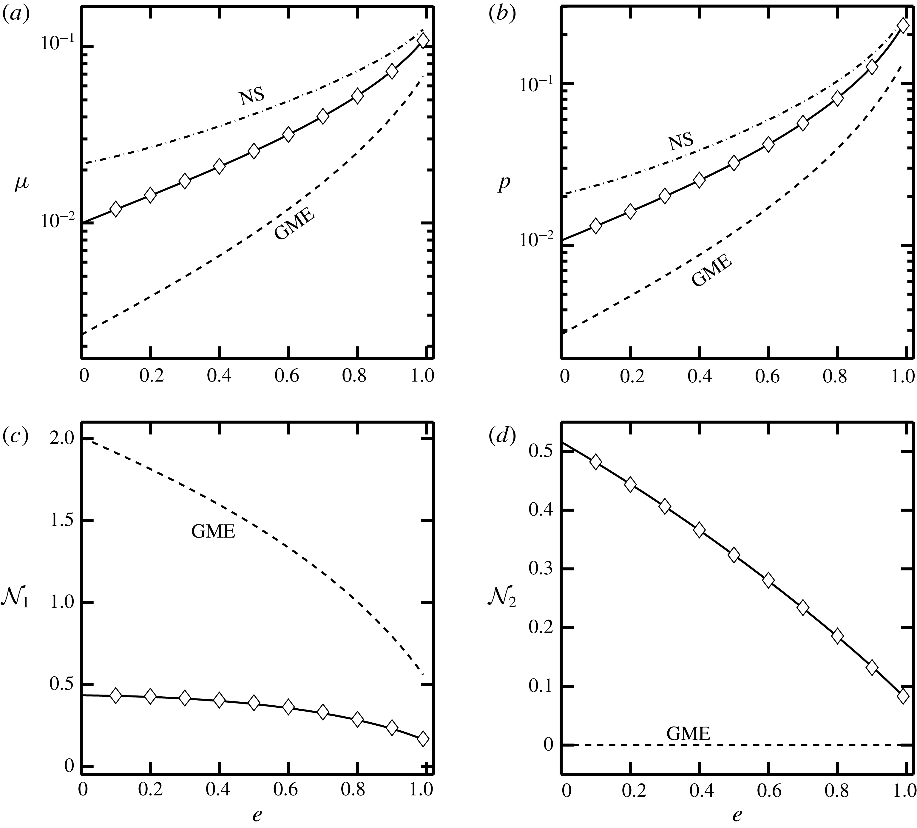
Figure 1 confirms the excellent agreement between the DSMC simulation data (marked by symbols) and the present theoretical predictions (solid lines) for (a) shear viscosity $\unicode[STIX]{x1D707}$ , (b) pressure $p$ , and (c) first ( ${\mathcal{N}}_{1}$ ) and (d) second ( ${\mathcal{N}}_{2}$ ) normal-stress differences at $St=10$ . The dot-dashed and dashed lines correspond to the NS order theory (Garzo et al. Reference Garzo, Tenneti, Subramaniam and Hrenya2012) and the 13-moment theory based on Grad’s moment expansion (dubbed ‘GME’ theory (Sangani et al. Reference Sangani, Mo, Tsao and Koch1996)), respectively. It is clear that the present theory fares remarkably well in correctly predicting both NS ( $\unicode[STIX]{x1D707}$ and $p$ ) and non-Newtonian ( ${\mathcal{N}}_{1}$ and ${\mathcal{N}}_{2}$ ) transport coefficients over the whole range of restitution coefficients even for a Stokes number of $St=10$ at a finite density of $\unicode[STIX]{x1D708}=0.2$ . According to the GME theory, ${\mathcal{N}}_{2}=0$ (see figure 1 d) and ${\mathcal{N}}_{1}>0$ (see figure 1 c), but the latter is overpredicted (compared to the simulation data) by a factor of approximately 2–4 over the whole range of restitution coefficients. The overall agreement in figure 1 between the AME theory and the simulation data also holds excellently for higher values of $St$ (see § 4.2).

Figure 1.

Predictions of AME (solid lines) for (a) shear viscosity, (b) pressure, (c)  ${\mathcal{N}}_{1}$ and (d)  ${\mathcal{N}}_{2}$ for the whole range of the restitution coefficient $e$ ; the particle volume fraction is set to $\unicode[STIX]{x1D708}=0.2$ and the Stokes number is $St=10$ (i.e.  $St_{d}\approx 2.5$ ). The dashed lines represent the GME theory of Sangani et al. (Reference Sangani, Mo, Tsao and Koch1996), the dot-dashed lines in panels (a) and (b) represent the NS order theory of Garzo et al. (Reference Garzo, Tenneti, Subramaniam and Hrenya2012) and the symbols correspond to DSMC data.

Before presenting the results on the $St$ dependence of transport coefficients, it is interesting to compare our predictions in figure 1 with previous works on dilute suspensions. Referring to figure 12 of Saha & Alam (Reference Saha and Alam2017), which corresponds to a particle volume fraction of $\unicode[STIX]{x1D708}=0.01$ with other parameters as in figure 1, we recall that the quantitative predictions of the GME theory were found to be comparable to those of the AME theory for both the shear viscosity and the first normal-stress difference even for highly inelastic particles with $e\geqslant 0.5$ . On increasing the volume fraction to a modest value of $\unicode[STIX]{x1D708}=0.2$ , however, the predictions of the GME theory become poor at all restitution coefficients, as demonstrated in figure 1. In contrast, the predictions of the present theory (including the second normal-stress difference) remain superior at finite densities over the whole range of restitution coefficients.

4.2 Predictions at large and small Stokes numbers

Since the Stokes number and particle Reynolds number are related via $St=(2/9)(\unicode[STIX]{x1D70C}_{p}/\unicode[STIX]{x1D70C}_{g})Re_{p}$ , the limit of rapid granular suspension ( $St\gg 1$ ) is easily satisfied since $\unicode[STIX]{x1D70C}_{p}/\unicode[STIX]{x1D70C}_{g}\gg 1$ in most gas–solid systems; it is also possible to reach the limit of $St\sim O(Re_{p}\ll 1)$ if $\unicode[STIX]{x1D70C}_{p}\sim \unicode[STIX]{x1D70C}_{g}$ , which corresponds to a liquid–solid suspension. Of course, the many-body hydrodynamic interactions are important in the latter limit, all of which are not incorporated in the present theory, as pointed out in § 2. Given that the theory and the DSMC simulation have identical assumptions, in this section our primary goals are (i) to analyse the performance of the present theory over existing theories over a wide range of $St$ for different values of $\unicode[STIX]{x1D708}$ and $e$ , and (ii) to determine to what extent the theory can be used in the small- $St$ regime. The effect of full hydrodynamic interactions on the predicted rheology will be discussed in §§ 5.1 and 5.2.

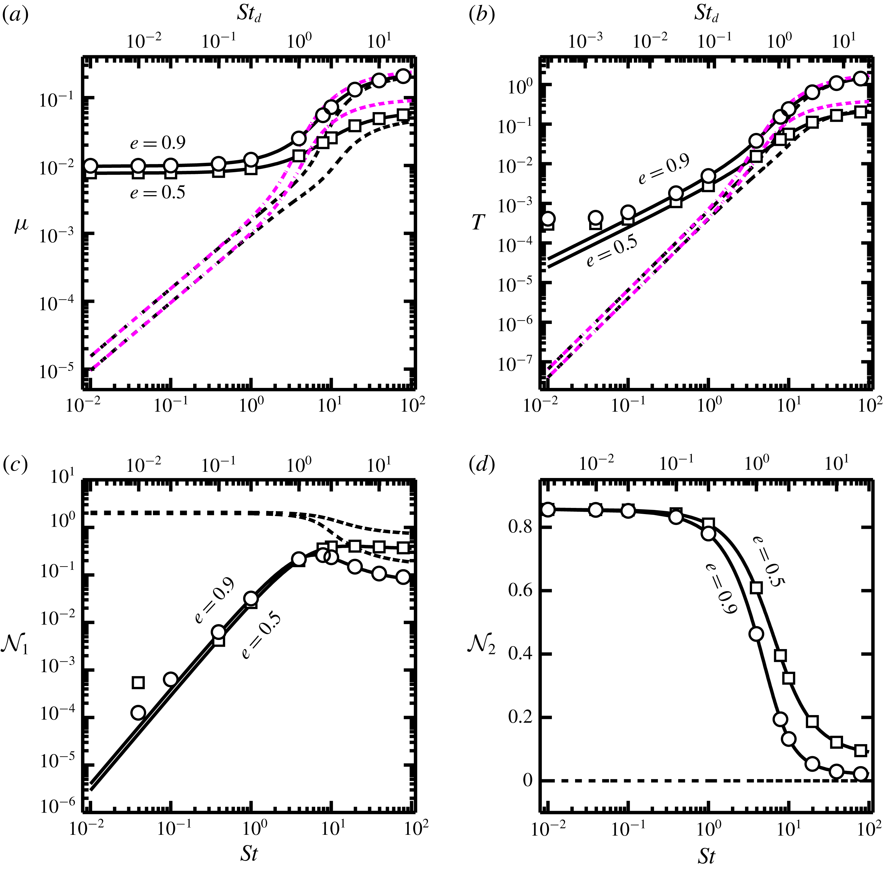
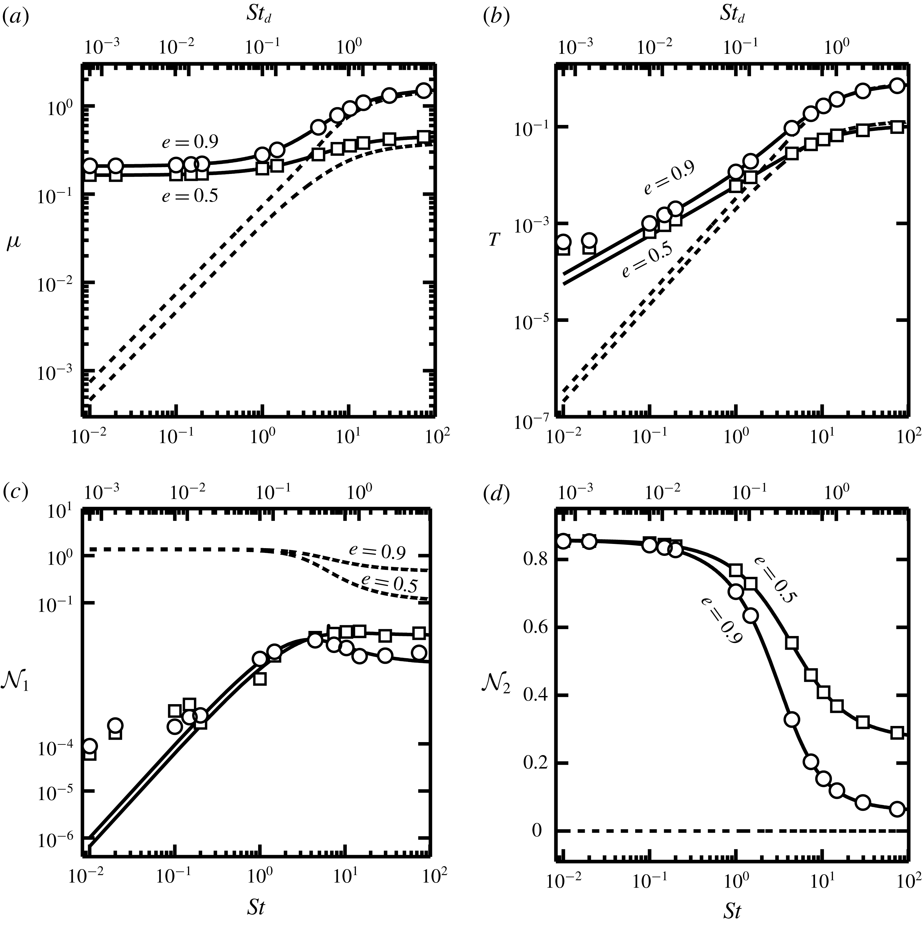
Figures 2 and 3 display the $St$ dependence of (a) particle-phase shear viscosity $\unicode[STIX]{x1D707}$ , (b) granular temperature $T$ , and (c) first ( ${\mathcal{N}}_{1}$ ) and (d) second ( ${\mathcal{N}}_{2}$ ) normal-stress differences, for particle volume fractions of $\unicode[STIX]{x1D708}=0.2$ and $0.5$ , respectively; the related range of the effective Stokes number $St_{d}$ (2.12) is marked on the top horizontal axis in each panel. Focusing on the high- $St$ regime in figures 2 and 3, it is seen that the predictions of the GME theory (Sangani et al. Reference Sangani, Mo, Tsao and Koch1996) for all fields become poorer with decreasing restitution coefficient $e$ . In particular, the first normal-stress difference (figures 2 c and 3 c) is overpredicted in the GME theory and its disagreement with the simulation data increases significantly in a denser suspension, as can be seen from a comparison between figures 2(c) ( $\unicode[STIX]{x1D708}=0.2$ ) and 3(c) ( $\unicode[STIX]{x1D708}=0.5$ ) at $St\gg 1$ – this disagreement is noteworthy despite the negligible effects of hydrodynamic interactions in the high- $St$ regime. In contrast, the present theory can quantitatively predict all transport coefficients ( $\unicode[STIX]{x1D707}$ , ${\mathcal{N}}_{1}$ and ${\mathcal{N}}_{2}$ ) over a large range of Stokes numbers $St\in (0.01,100)$ at $\unicode[STIX]{x1D708}=0.2$ (figure 2) and $0.5$ (figure 3) even for highly inelastic ( $e=0.5$ ) particles.

Figure 2.

Variations of the (a) particle-phase shear viscosity $\unicode[STIX]{x1D707}$ , (b) granular temperature $T$ , and (c) first $({\mathcal{N}}_{1})$ and (d) second $({\mathcal{N}}_{2})$ normal-stress differences plotted against Stokes number $St$ ; the axis on the top represents the effective Stokes number $St_{d}$ ; see (2.12). The solid and dashed lines, respectively, denote the present theory and the GME theory of Sangani et al. (Reference Sangani, Mo, Tsao and Koch1996); the magenta dot-dashed line refers to the NS theory of Garzo et al. (Reference Garzo, Tenneti, Subramaniam and Hrenya2012); the circles ( $e=0.9$ ) and squares ( $e=0.5$ ) denote DSMC results. The particle volume fraction is set to $\unicode[STIX]{x1D708}=0.2$ .

Figure 3.

Same as figure 2, but for a dense suspension with particle volume fraction $\unicode[STIX]{x1D708}=0.5$ .

In the small- $St$ regime, the predictions for shear viscosity (figures 2 a and 3 a), granular temperature (figures 2 b and 3 b) and ${\mathcal{N}}_{1}$ (figures 2 c and 3 c) based on the GME theory are qualitatively different from those of the present theory and DSMC simulation. For example, at $St\rightarrow 0$ , the scaled viscosity (and also pressure) approaches some constant value in the present theory, while it decays linearly with $St$ in GME theory. In figure 2(a,b), the dot-dashed lines represent the NS theory (Garzo et al. Reference Garzo, Tenneti, Subramaniam and Hrenya2012) which closely follow the GME theory in the small- $St$ limit ( $St\ll 1$ ). Note that the quantitative predictions of the NS theory deteriorate with decreasing $e$ in the high- $St$ limit – this is a well-known defect of all NS models (Saha & Alam Reference Saha and Alam2016; Alam & Saha Reference Alam and Saha2017).

Let us now discuss about the behaviour of two normal-stress differences in terms of the second-moment anisotropy. From the definition of the kinetic stress $\unicode[STIX]{x1D617}_{\unicode[STIX]{x1D6FC}\unicode[STIX]{x1D6FD}}^{k}=\unicode[STIX]{x1D70C}M_{\unicode[STIX]{x1D6FC}\unicode[STIX]{x1D6FD}}$ and employing (3.6), the anisotropies of the second-moment tensor can be expressed as

(4.3a-c ) $$\begin{eqnarray}\displaystyle \unicode[STIX]{x1D719}=\frac{1}{2}\tan ^{-1}\left(\frac{\unicode[STIX]{x1D617}_{yy}^{k}-\unicode[STIX]{x1D617}_{xx}^{k}}{2\unicode[STIX]{x1D617}_{xy}^{k}}\right),\quad \unicode[STIX]{x1D702}=\frac{-\unicode[STIX]{x1D617}_{xy}^{k}}{p^{k}\cos 2\unicode[STIX]{x1D719}},\quad \unicode[STIX]{x1D706}^{2}=\frac{(\unicode[STIX]{x1D617}_{xx}^{k}+\unicode[STIX]{x1D617}_{yy}^{k})}{2p^{k}}-1,\qquad & & \displaystyle\end{eqnarray}$$

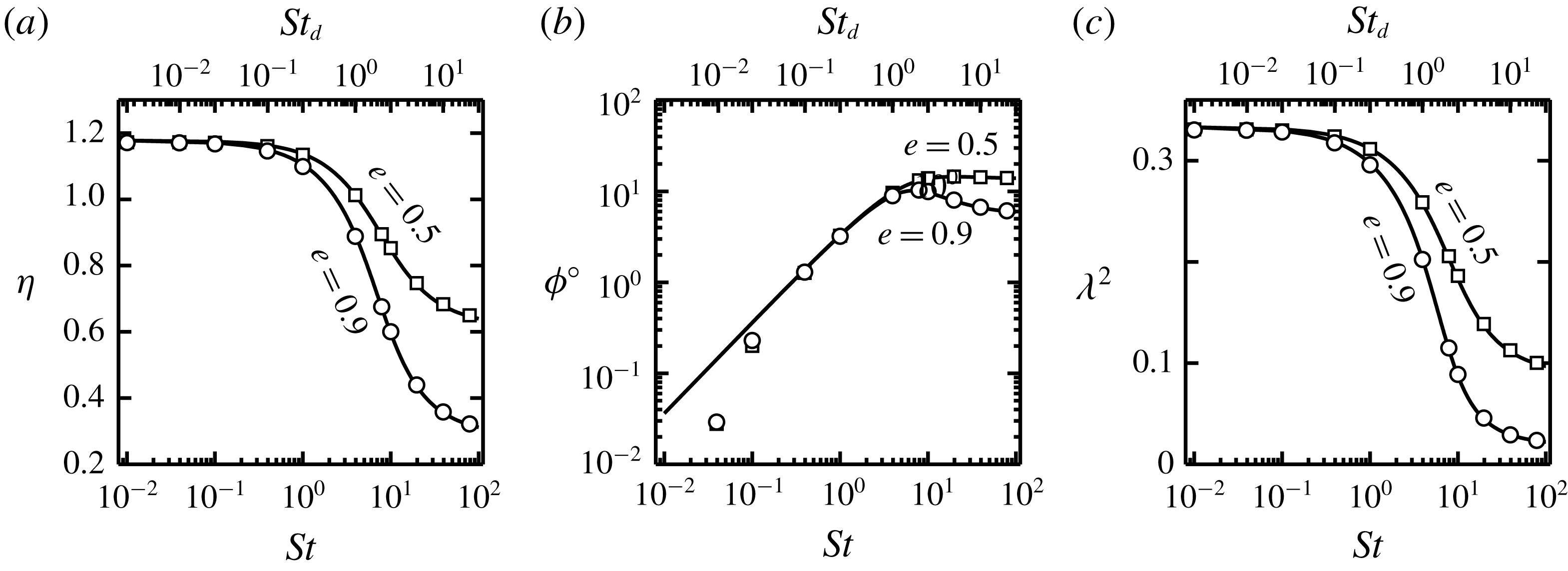
where $p^{k}=\unicode[STIX]{x1D617}_{\unicode[STIX]{x1D6FC}\unicode[STIX]{x1D6FC}}^{k}/3$ is the kinetic pressure. From the simulation data on $\unicode[STIX]{x1D617}_{\unicode[STIX]{x1D6FC}\unicode[STIX]{x1D6FD}}^{k}$ , three anisotropy parameters have been calculated from (4.3), and their variations with $St$ and $St_{d}$ are shown by symbols in figure 4(a–c), with solid lines representing theoretical predictions at $\unicode[STIX]{x1D708}=0.2$ . The related results at a higher volume fraction of $\unicode[STIX]{x1D708}=0.5$ look similar (and hence are not displayed) – in general, the magnitudes of ( $\unicode[STIX]{x1D702},\unicode[STIX]{x1D719},\unicode[STIX]{x1D706}^{2}$ ) decrease with increasing density and vice versa in the high- $St$ regime. From figure 4 we find that $\unicode[STIX]{x1D719}\rightarrow 0$ and $\unicode[STIX]{x1D706}^{2}\rightarrow 1/3$ at $St\rightarrow 0$ , and hence it follows from (4.3) that

(4.4a-c ) $$\begin{eqnarray}\displaystyle \unicode[STIX]{x1D617}_{xx}^{k}=\unicode[STIX]{x1D617}_{yy}^{k},\quad \unicode[STIX]{x1D702}=-\unicode[STIX]{x1D617}_{xy}^{k}/p^{k}\approx 1.2,\quad T_{z}/T=1-2\unicode[STIX]{x1D706}^{2}\rightarrow 1/3. & & \displaystyle\end{eqnarray}$$

The first normal-stress difference can be expressed in terms of the anisotropy parameters (Saha & Alam Reference Saha and Alam2016), ${\mathcal{N}}_{1}\propto \unicode[STIX]{x1D702}\sin 2\unicode[STIX]{x1D719}$ , and hence it vanishes at $St\rightarrow 0$ due to $\sin 2\unicode[STIX]{x1D719}\rightarrow 0$ (see figure 4 b) as confirmed in figures 2(c) and 3(c). Therefore, according to the present theory, the vanishing of ${\mathcal{N}}_{1}$ at $St\rightarrow 0$ is tied to the collinearity ( $\unicode[STIX]{x1D719}\rightarrow 0$ ) of the eigendirections of the second-moment and shear tensors in the same limit. On the other hand, the order-one value of the second normal-stress difference at $St\rightarrow 0$ in figures 2(d) and 3(d) is tied to the fact that the temperature ( $T_{z}$ ) in the vorticity direction is much different from those in the shear plane since $T_{x}+T_{y}=8T_{z}$ in this limit.

Figure 4.

Variations with $St$ or $St_{d}$ of the second-moment anisotropy parameters: (a)  $\unicode[STIX]{x1D702}$ (temperature anisotropy in the shear plane, equation (3.7)), (b)  $\unicode[STIX]{x1D719}$ (the non-coaxiality angle, equation (3.8)) and (c)  $\unicode[STIX]{x1D706}^{2}$ (the excess temperature, equation (3.9)) for $\unicode[STIX]{x1D708}=0.2$ .

Figure 5.

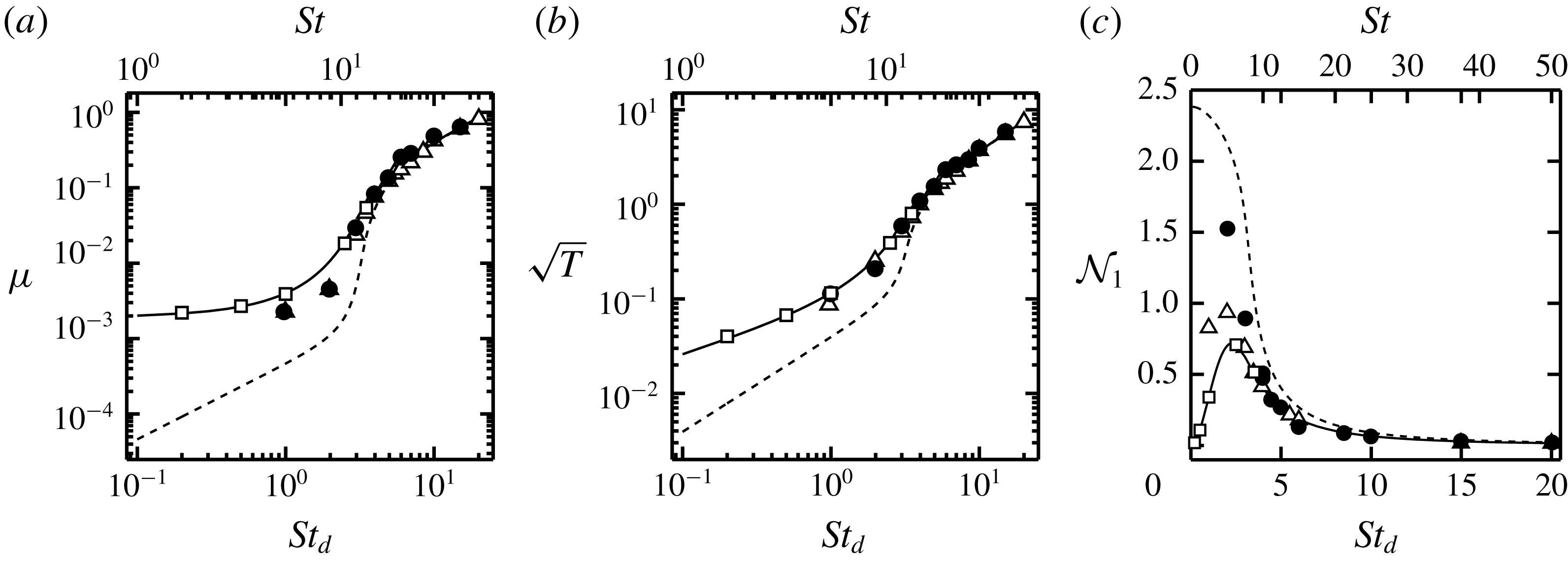
Comparison with the simulation data of Sangani et al. (Reference Sangani, Mo, Tsao and Koch1996) for $e=1$ and $\unicode[STIX]{x1D708}=0.1$ : (a) shear viscosity, (b) granular temperature and (c)  ${\mathcal{N}}_{1}$ . The filled circles and open triangles refer to their data with and without full hydrodynamic interactions, respectively; the open squares represent our DSMC data, which incorporate an effective drag term ( $\propto f_{diss}(\unicode[STIX]{x1D708})$ ) to update particle trajectories. The solid and dashed lines refer to the present theory and the GME theory of Sangani et al. (Reference Sangani, Mo, Tsao and Koch1996), respectively.

5.1 Effect of hydrodynamic interactions

Recall that the present theory does not include all many-body hydrodynamic interactions: the long-range hydrodynamic interactions and the short-range lubrication force are incorporated only via the viscous dissipation term (calculated with an isotropic Maxwellian distribution function) in the second-moment equation. However, (i) the effects of the anisotropic particle distribution function on hydrodynamic interactions, (ii) the fluid flow affecting the particle distribution function and (iii) the interactions due to shear-induced particle stresslet are neglected. Such detailed hydrodynamic interactions with non-Maxwellian velocity distribution for both the particle and gas phases may impact the effective viscous dissipation terms that are neglected in the present theory. In any case, to check the possible implications of detailed hydrodynamic interactions in simple shear, we compare our theory in figure 5 with the simulation data of Sangani et al. (Reference Sangani, Mo, Tsao and Koch1996) that includes all hydrodynamic interactions – this refers to the case of elastically colliding ( $e=1$ ) particles for a volume fraction of $\unicode[STIX]{x1D708}=0.1$ . The filled circles and open triangles refer to their data with and without full hydrodynamic interactions, respectively; the open squares represent our DSMC simulation data which incorporate hydrodynamic interactions only via the effective drag force (equations (2.8) and (2.9)). It is seen that both sets of simulation data for (a)  $\unicode[STIX]{x1D707}$ , (b)  $T$ and (c)  ${\mathcal{N}}_{1}$ overlap with each other as well as with two theories (AME and GME) at Stokes numbers of $St_{d}>5$ (i.e.  $St>10$ ). This implies that many-body hydrodynamic interactions do not noticeably affect the rheology of suspensions ( $e=1$ ) at moderate to high values of the Stokes number – this overall conclusion also holds at higher volume fractions (as confirmed from a comparison of our theory with the simulation data for $\unicode[STIX]{x1D708}=0.25$ and $0.45$ obtained from figures 12 and 13 of Sangani et al. (Reference Sangani, Mo, Tsao and Koch1996)).

Focusing on the small- $St$ regime of figure 5, we find that the quantitative predictions of the present theory are better than those of the GME theory even at a small value of $St_{d}=2$ . On the other hand, the simulation data with full hydrodynamic interactions (filled circles in figure 5 c) indicate that the first normal-stress difference increases with decreasing $St$ , reaching some finite value at $St=0$ – this is known to be a consequence of many-body hydrodynamic interactions in dense suspensions (Brady & Bossis Reference Brady and Bossis1988; Nott & Brady Reference Nott and Brady1994; Boyer, Pouliquen & Guazzelli Reference Boyer, Pouliquen and Guazzelli2011). The latter may be contrasted with the non-monotonic variation of ${\mathcal{N}}_{1}$ with $St$ , leading to ${\mathcal{N}}_{1}\rightarrow 0$ at $St\rightarrow 0$ , according to our theory and DSMC simulation. This non-monotonic variation is also captured by the simulation data of Sangani et al. (Reference Sangani, Mo, Tsao and Koch1996), marked by the open triangles in figure 5(c) – note that the latter simulations incorporate only an effective drag term to update particle trajectories as in our DSMC simulations.

It is interesting to note in figure 5(c) that the GME theory (dashed line) seems to predict the correct $St$ dependence of the hydrodynamic simulation data for ${\mathcal{N}}_{1}\neq 0$ at $St\rightarrow 0$ ; this prediction is incorrect. We have verified (Saha & Alam 2019, unpublished) that a consistent ‘second-order’ GME theory, which incorporates all second-order nonlinearities in the production and flux terms (equations (2.6) and (2.7)), yields a non-monotonic variation of ${\mathcal{N}}_{1}$ with $St$ , similar to the present predictions of the AME theory.

Based on above comparisons between simulation and theory, we conclude that the detailed hydrodynamic interactions must be included in the present theory to recover the correct behaviour of the first normal-stress difference at $St\rightarrow 0$ . In this regard, the (shear-induced) anisotropic microstructure is another missing link in the present theory which may be incorporated via the two-body distribution function.

5.2 Scaling of stress

Recall from figures 2(a) and 3(a) that the shear viscosity has two distinct plateaus at $St\gg 1$ (high viscosity) and $St\ll 1$ (low viscosity); the related variations of the particle pressure with $St$ (not shown) are similar. In the high- $St$ regime, the (dimensional) granular temperature scales like $T\sim \dot{\unicode[STIX]{x1D6FE}}^{2}\unicode[STIX]{x1D70E}^{2}$ (see figures 2 b and 3 b), yielding a quadratic dependence of stress with the shear rate (i.e.  $\unicode[STIX]{x1D617}_{xy}\sim \dot{\unicode[STIX]{x1D6FE}}^{2}$ ) – this is the well-known Bagnoldian or inertial scaling of stress that holds in rapid granular flows ( $St\rightarrow \infty$ ).

In the small- $St$ regime too, the present theory recovers the same inertial scaling of stress ( $\unicode[STIX]{x1D617}_{xy}\sim \dot{\unicode[STIX]{x1D6FE}}^{2}$ ), and the (dimensional) particle-phase viscosity has a linear dependence on the shear rate ( $\tilde{\unicode[STIX]{x1D707}}_{AME}\sim \dot{\unicode[STIX]{x1D6FE}}\sim St/\unicode[STIX]{x1D70F}_{vis}$ ). This can be understood from the energy balance equation by equating the shear work ( $\unicode[STIX]{x1D617}_{xy}\dot{\unicode[STIX]{x1D6FE}}$ ) with the viscous dissipation ( $\unicode[STIX]{x1D6E4}_{vis}=2\unicode[STIX]{x1D70C}T/\unicode[STIX]{x1D70F}_{vis}^{e}$ ) since inelastic dissipation is insignificant at $St\ll 1$ . This yields an expression for the shear stress as $\unicode[STIX]{x1D617}_{xy}\sim n\unicode[STIX]{x1D70E}\unicode[STIX]{x1D707}_{g}T/\dot{\unicode[STIX]{x1D6FE}}$ , which, together with the scaling for the temperature $T\sim St\dot{\unicode[STIX]{x1D6FE}}^{2}\unicode[STIX]{x1D70E}^{2}$ (figure 2 b), leads to $\unicode[STIX]{x1D617}_{xy}^{\,AME}\sim \unicode[STIX]{x1D70C}\dot{\unicode[STIX]{x1D6FE}}^{2}\unicode[STIX]{x1D70E}^{2}$ at $St\ll 1$ . This scaling holds also in DSMC simulations as is evident from the simulation data on the low-viscosity branch in figures 2(a) and 3(a). These predictions are at odds with the well-known viscous scaling of stress, $\lim _{St\rightarrow 0}\unicode[STIX]{x1D617}_{xy}\propto \unicode[STIX]{x1D707}_{g}\dot{\unicode[STIX]{x1D6FE}}$ , for Stokesian suspensions.

At a phenomenological level, the viscous scaling of stress can be recovered by incorporating the hydrodynamic contribution to the particle-phase stress tensor via $\unicode[STIX]{x1D64B}=\unicode[STIX]{x1D64B}^{k}+\unicode[STIX]{x1D64B}^{c}+\unicode[STIX]{x1D64B}^{h}$ . For low-Reynolds-number suspensions, Nott & Brady (Reference Nott and Brady1994) suggested an expression for the hydrodynamic stress:

(5.1) $$\begin{eqnarray}\displaystyle \unicode[STIX]{x1D64B}^{h}=\unicode[STIX]{x1D6F1}\unicode[STIX]{x1D644}+2\unicode[STIX]{x1D707}_{g}\unicode[STIX]{x1D707}_{r}(\unicode[STIX]{x1D708})\unicode[STIX]{x1D63F}+\unicode[STIX]{x1D707}_{g}\unicode[STIX]{x1D729}\,\boldsymbol{ : }\,\unicode[STIX]{x1D63F}, & & \displaystyle\end{eqnarray}$$

where $\unicode[STIX]{x1D6F1}$ is the particle pressure, $\unicode[STIX]{x1D63F}=(\unicode[STIX]{x1D735}\boldsymbol{u}+(\unicode[STIX]{x1D735}\boldsymbol{u})^{\dagger })/2$ is the strain-rate tensor, $\unicode[STIX]{x1D707}_{r}(\unicode[STIX]{x1D708})$ is the relative viscosity, which is an increasing function of the particle volume fraction, and $\unicode[STIX]{x1D729}$ is a fourth-rank tensor that takes care of normal-stress differences. In fact, (5.1) represents the dominant contribution to the particle stress tensor at $St\rightarrow 0$ . Neglecting normal-stress differences in (5.1) and plugging it into the energy balance (2.5) yields $T\sim \dot{\unicode[STIX]{x1D6FE}}^{2}\unicode[STIX]{x1D70E}^{2}$ – this is dubbed the ‘suspension’ temperature, which is tied with the non-affine motion of the particles. The above scaling is the same as that of Nott & Brady (Reference Nott and Brady1994), and would lead to a plateau in figure 2(b) at $St\rightarrow 0$ – of course, the stress scaling now remains viscous. A detailed analysis would require constitutive relations for the particle pressure $\unicode[STIX]{x1D6F1}=\unicode[STIX]{x1D6F1}_{0}+\unicode[STIX]{x1D707}_{g}p_{r}(\unicode[STIX]{x1D708})\dot{\unicode[STIX]{x1D6FE}}$ , the density dependence of the relative viscosity $\unicode[STIX]{x1D707}_{r}(\unicode[STIX]{x1D708})$ and the fourth-rank tensor $\unicode[STIX]{x1D729}$ (Nott & Brady Reference Nott and Brady1994; Lhuillier Reference Lhuillier2009; Guazzelli & Pouliquen Reference Guazzelli and Pouliquen2018). In summary, a phenomenological hybrid approach to incorporate the hydrodynamic stress in the manner of Nott & Brady (Reference Nott and Brady1994) could be useful to recover (i) the viscous scaling of stress and (ii) the correct shear-rate scaling of normal-stress differences at $St\rightarrow 0$ .

Figure 6.

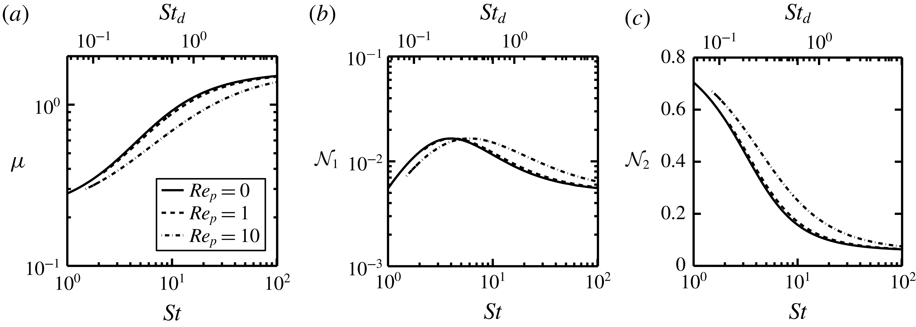
Effects of particle Reynolds number ( $Re_{p}$ ) on transport coefficients: (a) shear viscosity, and (b) first $({\mathcal{N}}_{1})$ and (c) second $({\mathcal{N}}_{2})$ normal-stress differences. The lines denote theoretical predictions for different values of $Re_{p}$ with a particle volume fraction of $\unicode[STIX]{x1D708}=0.5$ and $e=0.9$ .

5.3 Effect of fluid inertia

As clarified in § 2, all the above results are applicable strictly for zero-Reynolds-number ( $Re_{p}=0$ ) suspensions. In the context of the present theory, the possible effects of fluid inertia ( $Re_{p}>0$ ) on the particle-phase rheology can be ascertained via a modified viscous dissipation function (2.8). In this regard, an approximate expression for the dissipation function has been suggested by Verberg & Koch (Reference Verberg and Koch2006):

(5.2) $$\begin{eqnarray}\displaystyle f_{diss}(\unicode[STIX]{x1D708},\unicode[STIX]{x1D716}_{m};Re_{T})=f_{diss}(\unicode[STIX]{x1D708},\unicode[STIX]{x1D716}_{m};0)+\min \{K_{s}Re_{T},K_{l}Re_{T}+(K_{s}-K_{l})Re_{T}^{0}\}. & & \displaystyle\end{eqnarray}$$

Here $Re_{T}$ is the thermal Reynolds number based on the granular temperature

(5.3) $$\begin{eqnarray}\displaystyle Re_{T}=\frac{\unicode[STIX]{x1D70C}_{g}\unicode[STIX]{x1D70E}\sqrt{T}}{\unicode[STIX]{x1D707}_{g}}\equiv Re_{p}(\sqrt{T}/\dot{\unicode[STIX]{x1D6FE}}\unicode[STIX]{x1D70E}), & & \displaystyle\end{eqnarray}$$

with $Re_{p}=\unicode[STIX]{x1D70C}_{g}\dot{\unicode[STIX]{x1D6FE}}\unicode[STIX]{x1D70E}^{2}/\unicode[STIX]{x1D707}_{g}$ being the particle Reynolds number, and

(5.4) $$\begin{eqnarray}\displaystyle Re_{T}^{0}=(0.1729-0.3416\unicode[STIX]{x1D708}+0.5973\unicode[STIX]{x1D708}^{2})^{-1} & & \displaystyle\end{eqnarray}$$

is a transition Reynolds number that demarcates two regimes defined via

(5.5a ) $$\begin{eqnarray}\displaystyle & \displaystyle K_{s}(\unicode[STIX]{x1D708})=\unicode[STIX]{x1D708}(3.3237-12.253\unicode[STIX]{x1D708}+32.97\unicode[STIX]{x1D708}^{2}), & \displaystyle\end{eqnarray}$$

(5.5b ) $$\begin{eqnarray}\displaystyle & \displaystyle K_{l}(\unicode[STIX]{x1D708})=\unicode[STIX]{x1D708}(2.0233-6.4742\unicode[STIX]{x1D708}+19.773\unicode[STIX]{x1D708}^{2}), & \displaystyle\end{eqnarray}$$

$Re_{T}<Re_{T}^{0}$

$Re_{T}>Re_{T}^{0}$

$f_{diss}(Re_{p})$

We have incorporated (5.2) in the second-moment balance equations (3.12)–(3.15) that are solved for specified values of ( $Re_{p},\unicode[STIX]{x1D708},e,St$ ). Figure 6 shows the influence of $Re_{p}$ on transport coefficients predicted by the present theory; the particle volume fraction is set to $\unicode[STIX]{x1D708}=0.5$ and the restitution coefficient is $e=0.9$ . The qualitative behaviour of each transport coefficient with varying $St$ remains the same as that for $Re_{p}=0$ and also at other values of $\unicode[STIX]{x1D708}$ . It is seen that the shear viscosity decreases but the normal-stress differences are enhanced with increasing fluid inertia at $Re_{p}=10$ , and the changes are negligible at $Re_{p}=1$ as well as at $St<1$ (not shown). Increased viscous dissipation with increasing $Re_{p}$ is responsible for the reduction of the particle-phase viscosity. On the whole, our predictions in § 4 would remain largely unaffected at small finite values of the particle Reynolds number.