2. Problem formulation

We place a plane disk of finite radius $R$ into an infinite region filled with an initially stagnant fluid. At time $\hat {t}=0$, the disk is brought into rotation around the axis perpendicular to its surface and passing through its centre, at a constant angular velocity $\varOmega$. Owing to the action of viscous forces, the fluid particles adjacent to the disk start to rotate, but their trajectories are not circular: they also tend to move away from the axis of rotation due to inertial forces. In addition to the layers of rotating fluid, developing above and below the disk, a jet is generated from the rim of the rotating disk, and it propagates radially away as time increases.

Because of the topology of the flow, it is convenient to use cylindrical polar coordinates $(\hat {r},\varPhi ,\hat {z})$ such that the origin $O$ coincides with the centre of the disk, and that the axis $(O,\hat {z})$ coincides with the axis of rotation of the disk. This coordinate system is presented in figure 1. Thus, a point $M$ of space may be located by the three coordinates $\hat {r}$, $\varPhi$ and $\hat {z}$ such that $\hat {z}$ is the distance between $M$ and $M'$, where $M'$ is the projection of $M$ to the $(\hat {r},\varPhi )$ plane, $\hat {r}$ measures the distance from $M$ to its projection on the axis of rotation $(O\hat {z})$ while $\varPhi$ is the angle between the $\hat {x}$ axis and the line $(OM')$. The unit vectors along the $\hat {r}$, $\varPhi$ and $\hat {z}$ axes are denoted respectively by $\boldsymbol {e}_{\boldsymbol {r}}$, $\boldsymbol {e}_{\boldsymbol {\varPhi }}$ and $\boldsymbol {e}_{\boldsymbol {z}}$.

Figure 1.

Cylindrical coordinates.

The problem is obviously axisymmetric as the solution is invariant with respect to an arbitrary rotation through an angle $\Delta \varPhi$, so all the flow quantities are independent of the circumferential coordinate $\varPhi$:

(2.1)\begin{equation} \frac{\partial }{\partial \varPhi}=0. \end{equation}

Moreover, as the flow is axisymmetric, we study it for positive $\hat {r}$ only, as the solution for negative $\hat {r}$ may be recovered by symmetry with respect to the axis $(O,\hat {z})$. Besides, the flow is symmetric with respect to the plane containing the disk, so we study the problem for positive $\hat {z}$ only. The solution for negative $\hat {z}$ may be deduced by symmetry.

Our goal is to solve the unsteady boundary-layer equations dictating the behaviour of the flow. They are not only parabolic; they have elements of hyperbolicity due to the sub-hyperbolic operator

(2.2)\begin{equation} \frac{\partial \hat{u}}{\partial \hat{t}}+\hat{u}\frac{\partial \hat{u}}{\partial \hat{r}} \end{equation}

in the momentum equation (with $\hat {u}$ being the radial velocity component here). Because of the parabolic and hyperbolic natures of the boundary-layer equations, they are said to be of mixed type. It is because of their hyperbolic feature that we theoretically expect a jet to develop and propagate radially away as time increases.

We consider that the fluid is viscous, incompressible and Newtonian, and we neglect the body forces acting on the fluid such as gravity. Let us denote by $\rho$, $\mu$ and $\nu$ the density, dynamic viscosity and kinematic viscosity, respectively. The quantity $p_\infty$ corresponds to the pressure in the stagnant part of the fluid. We also introduce $\hat {u}$, $\hat {v}$, $\hat {w}$ and $\hat {p}$ as the radial, circumferential and axial components of the velocity, and the pressure, respectively. The hat stands for dimensional quantities. The flow is described by the unsteady Navier–Stokes equations written in cylindrical polar coordinates:

(2.3a)\begin{gather} \frac{\partial \hat{u}}{\partial \hat{t}}+\hat{u}\frac{\partial \hat{u}}{\partial \hat{r}}+\hat{w}\frac{\partial \hat{u}}{\partial \hat{z}}-\frac{\hat{v}^2}{\hat{r}}={-}\frac{1}{\rho}\frac{\partial \hat{p}}{\partial \hat{r}}+\nu\left(\frac{\partial ^2\hat{u}}{\partial \hat{z}^2}+\frac{\partial ^2\hat{u}}{\partial \hat{r}^2}+\frac{1}{\hat{r}}\frac{\partial \hat{u}}{\partial \hat{r}}-\frac{\hat{u}}{\hat{r}^2}\right), \end{gather}

(2.3b)\begin{gather}\frac{\partial \hat{v}}{\partial \hat{t}}+\hat{u}\frac{\partial \hat{v}}{\partial \hat{r}}+\hat{w}\frac{\partial \hat{v}}{\partial \hat{z}}+\frac{\hat{u}\hat{v}}{\hat{r}}=\nu\left(\frac{\partial ^2\hat{v}}{\partial \hat{z}^2}+\frac{\partial ^2\hat{v}}{\partial \hat{r}^2}+\frac{1}{\hat{r}}\frac{\partial \hat{v}}{\partial \hat{r}}-\frac{\hat{v}}{\hat{r}^2}\right), \end{gather}

(2.3c)\begin{gather}\frac{\partial \hat{w}}{\partial \hat{t}}+\hat{u}\frac{\partial \hat{w}}{\partial \hat{r}}+\hat{w}\frac{\partial \hat{w}}{\partial \hat{z}}={-}\frac{1}{\rho}\frac{\partial \hat{p}}{\partial \hat{z}}+\nu\left(\frac{\partial ^2\hat{w}}{\partial \hat{z}^2}+\frac{\partial ^2\hat{w}}{\partial \hat{r}^2}+\frac{1}{\hat{r}}\frac{\partial \hat{w}}{\partial \hat{r}}\right), \end{gather}

(2.3d)\begin{gather}\frac{\partial \hat{u}}{\partial \hat{r}}+\frac{\partial \hat{w}}{\partial \hat{z}}+\frac{\hat{u}}{\hat{r}}=0. \end{gather}

We must formulate boundary conditions in order to get a full description of the problem.

As we discussed earlier, a layer of rotating fluid is formed above and below the rotating disk due to the action of viscous forces, and the fluid particles adjacent to the disk surface follow its rotation, which is why the no-slip condition must be satisfied on the disk surface. Besides, the impermeability condition also holds as no fluid particle will flow through the disk. Hence, for all $\hat {t} \geqslant 0$,

(2.3e)\begin{equation} \hat{v}=\varOmega\hat{r},\ \hat{u}=\hat{w}=0, \quad \textrm{at} \ \hat{z}=0,\ \hat{r} \in [0,R]. \end{equation}

On the surface of the jet propagating in the radial direction away from the disk rim, the symmetry conditions hold:

(2.3f)\begin{equation} \hat{w}=\frac{\partial \hat{u}}{\partial \hat{z}}=\frac{\partial \hat{v}}{\partial \hat{z}}=0, \quad \textrm{at}\ \hat{z}=0,\ \hat{r}>R. \end{equation}

Far from the disk, the fluid is stagnant:

(2.3g)\begin{equation} \hat{v}=0, \quad \textrm{at}\ \hat{r}^2+\hat{z}^2=\infty. \end{equation}

The motion of the fluid in the radial direction is caused by the centrifugal forces $\hat {v}^2/\hat {r}^2$, which is the fourth term on the left-hand side of the radial momentum equation (2.3a). According to that and to (2.3g), far from the disk the centrifugal term vanishes, so we deduce that the radial component of the velocity is equal to 0 outside the layer of rotating fluid:

(2.3h)\begin{equation} \hat{u}=0, \quad \textrm{at}\ \hat{r}^2+\hat{z}^2=\infty. \end{equation}

Regarding the axial velocity component $\hat {w}$, it is determined with the help of the continuity equation (2.3d). The axial momentum equation (2.3c) is kept to compute the pressure field $\hat {p}$. Thus, we do not need a boundary condition for $\hat {w}$ for large values of $\hat {z}$. Since the flow is at rest far from the disk, the pressure there is kept constant:

(2.3i)\begin{equation} \hat{p}=p_\infty, \quad \textrm{at}\ \hat{r}^2+\hat{z}^2=\infty. \end{equation}

On the axis of rotation of the disk, the fluid particles cannot move across, and a symmetry condition holds:

(2.3j)\begin{equation} \hat{u}=\hat{v}=\frac{\partial \hat{w}}{\partial \hat{r}}=0, \quad \textrm{at}\ \hat{r}=0. \end{equation}

The boundary-value problem (2.3a)–(2.3j) is now fully established. It describes the flow motion everywhere in the domain for all values of $\hat {t}\geqslant 0$. When the disk starts rotating at $\hat {t}=0$ with a constant angular velocity $\varOmega$, a layer of rotating fluid develops adjacent to the disk. Its thickness, which was initially equal to $0$, grows as time increases. If $\varOmega$ is kept constant for long enough, a steady state is reached: then the sought flow functions no longer vary in time, including the thickness of the rotating fluid layer. Regarding the unsteady solution of the boundary-value problem (2.3a)–(2.3j), one must distinguish two flow regimes depending on the order of magnitude of time $\hat {t}$. The first one is when $\hat {t}$ is small, such that the convective terms of the momentum equations (2.3a), (2.3b) and (2.3c) are negligible as compared to the local accelerations $\partial \hat {u}/\partial \hat {t}$, $\partial \hat {v}/\partial \hat {t}$ and $\partial \hat {w}/\partial \hat {t}$, respectively. A second regime must be considered when $\hat {t}$ becomes larger and the convective terms can no longer be neglected. Instead, they are of same order as the local accelerations. For the sake of understanding, the former one may be called regime $a$, while the second one will be called regime $b$. During both regimes, the layer of moving fluid may be divided into two regions: a thin viscous layer adjacent to the disk surface and the jet axis $\hat {z}=0$, and an outer inviscid layer whose thickness is of order $\hat {r}$ and where the entrainment effect takes place. A detailed introduction of these two regions is presented later on. For now, the order of magnitudes of $\hat {t}$ corresponding to both regimes $a$ and $b$ may be determined by performing an inspection analysis of the sought flow functions in the viscous layer of rotating fluid.

For $\hat {t}\geqslant 0$, the circumferential velocity component must satisfy the no-slip condition (2.3e) on the disk surface, and it tends to $0$ far from the disk according to the boundary condition (2.3g). Thus,

(2.4)\begin{equation} \hat{v}\sim\varOmega\hat{r}. \end{equation}

Since the fluid is brought into motion due to the action of viscous forces, then the thickness $\hat {z}$ of the viscous layer of fluid developing when the disk starts rotating may be estimated by balancing the local acceleration with the viscous term in the circumferential momentum equation (2.3b):

(2.5)\begin{equation} \frac{\partial \hat{v}}{\partial \hat{t}}\sim\nu\frac{\partial ^2\hat{v}}{\partial \hat{z}^2}. \end{equation}

It results that

(2.6)\begin{equation} \hat{z}\sim\sqrt{\nu\hat{t}}. \end{equation}

As expected, $\hat {z}$ tends to $0$ during regime $a$ (that is, when $\hat {t}$ is small) and $\hat {z}\ll \hat {r}$. During regime $b$ when $\hat {t}$ becomes larger, $\hat {z}$ increases and satisfies $\hat {z}\sim \hat {r}$.

The movement of fluid in the radial direction is dictated by the centrifugal term $\hat {v}^2/\hat {r}$, so this term must be comparable with the local acceleration in the radial momentum equation (2.3a). Using (2.4), we deduce that

(2.7)\begin{equation} \hat{u}\sim\varOmega^2\hat{r}\hat{t}. \end{equation}

The axial velocity component may be deduced from the continuity equation (2.3d) by applying the principle of least degeneration:

(2.8)\begin{equation} \hat{w}\sim\varOmega^2\nu^{1/2}\hat{t}^{3/2}. \end{equation}

Finally, the pressure variation must be estimated. One can find the pressure estimate by studying the flow in the outer inviscid region where the entrainment effect takes place. Relation (2.8) is also valid in the outer region because the entrainment effect causes an injection of fluid into the viscous layer, so the axial velocity component is of the same order in both regions. We balance the pressure gradient and the local acceleration in the axial momentum equation (2.3c). Substitution of (2.8) and taking into account that in the inviscid region $\hat {z}\sim \hat {r}$, it leads to

(2.9)\begin{equation} \hat{p}-p_\infty\sim\rho\varOmega^2\hat{r}\sqrt{\nu\hat{t}}. \end{equation}

Thus, estimates of all flow quantities in the viscous layer have been determined, and they are all valid for regime $a$. The order of magnitude of $\hat {t}$ during regime $b$ can be found by balancing the convective terms with the local acceleration in the radial momentum equation (2.3a). Using (2.7), it results that during regime $b$

(2.10)\begin{equation} \hat{t}\sim\frac{1}{\varOmega}. \end{equation}

Therefore, immediately after the disk is brought into rotation and as long as $\hat {t}\ll 1/\varOmega$, the flow is under regime $a$, implying that the convective terms are disregarded. Then, $\hat {t}$ keeps increasing, and once $\hat {t}\sim 1/\varOmega$, regime $b$ is reached and the convective terms become comparable with the local acceleration. If $\hat {t}$ keeps increasing further, then the steady state is reached, and we shall see later that the solution satisfies the solution of the von Kármán (Reference von Kármán1921) flow for $|\hat {r}|\leqslant 1$. For now, we study both regimes $a$ and $b$.

Let us start with regime $a$ when $\hat {t}$ is small, that is, in the limit as $\hat {t}\ll 1/\varOmega$. We shall find an analytical solution during regime $a$ in the viscous layer for $|\hat {r}|\leqslant 1$. We introduce the dimensionless quantities $t$, $r$, $z$, $u$, $v$, $w$ and $p$ based on (2.4), (2.6), (2.7), (2.8) and (2.9):

(2.11)\begin{equation} \left.\begin{gathered} \hat{t}=\alpha t,\quad \hat{r}=R r,\quad \hat{z}=\sqrt{\nu\alpha}z, \\ \hat{u}=\varOmega^2R\alpha u,\quad \hat{v}=\varOmega R v,\quad \hat{w}=\varOmega^2\nu^{1/2}\alpha^{3/2}w, \\ \hat{p}-p_\infty=\rho\varOmega^2R\sqrt{\nu\alpha}p. \end{gathered}\right\} \end{equation}

Substituting (2.11) into (2.3a)–(2.3d), and assuming that $\alpha \ll 1/\varOmega$, we arrive at the conclusion that

(2.12a)\begin{gather} \frac{\partial u}{\partial t}-\frac{v^2}{r}=\frac{\partial ^2u}{\partial z^2}, \end{gather}

(2.12b)\begin{gather}\frac{\partial v}{\partial t}=\frac{\partial ^2v}{\partial z^2}, \end{gather}

(2.12c)\begin{gather}\frac{\partial p}{\partial z}=0, \end{gather}

(2.12d)\begin{gather}\frac{\partial u}{\partial r}+\frac{\partial w}{\partial z}+\frac{u}{r}=0. \end{gather}

We notice that the centrifugal term in the circumferential momentum equation (2.12b) has been disregarded due to its small order of magnitude in the limit as $\hat {t}\ll 1/\varOmega$. However, the centrifugal term in the radial momentum equation (2.12a) is of the same order as the local acceleration, and so it cannot be neglected as the solution of this equation without the term $v^2/r$ would be $u=0$, which is a contradiction. The system of (2.12a)–(2.12d) with the corresponding boundary conditions (2.3e)–(2.3j) may be solved analytically. Let us start with the circumferential equation (2.12b). Guided by (2.4), we find that the solution for $v$ has the form

(2.13)\begin{equation} v=rF_\varPhi(t,z). \end{equation}

Consequently, substitution of $v$ into the circumferential momentum equation (2.12b) allows us to rewrite it and its related boundary conditions as a boundary-value problem in the unknown $F_\varPhi$, similar to the one-dimensional heat equation:

(2.14a)\begin{gather} \frac{\partial F_\varPhi}{\partial t}=\frac{\partial ^2F_\varPhi}{\partial z^2}, \end{gather}

(2.14b)\begin{gather}F_\varPhi=1, \quad \textrm{at } z=0, \end{gather}

(2.14c)\begin{gather}F_\varPhi=0, \quad \textrm{at } z=\infty, \end{gather}

(2.14d)\begin{gather}F_\varPhi=0, \quad \textrm{at } t=0 \textrm{ except at } z=0. \end{gather}

The boundary-value problem (2.14) can be solved by considering the following argument: since the thickness $\hat {z}$ of the viscous layer of rotating fluid is small as compared to the variable $\hat {r}$ (we recall that during regime $a$, $\hat {z}\sim \sqrt {\nu \hat {t}}$ and that $\hat {r}\sim R$), one can consider that there is no characteristic length scale involved in the problem under the assumption $\hat {t}\ll 1/\varOmega$. Furthermore, there is no characteristic time scale which can be assigned to the problem. Therefore, the solution must admit a self-similar form. This means that if the solution is known at one specific time $\hat {t}$, then the solution at another time may be found by making use of affine transformations. Let

(2.15)\begin{equation} F_\varPhi=\mathcal{F}(t,z) \end{equation}

be the solution of (2.14). We write the affine transformations by introducing the constants $A$, $B$ and $C$ such that

(2.16a–c)\begin{equation} t=A\bar{t},\quad z=B\bar{z},\quad F_\varPhi=C\bar{F}_\varPhi. \end{equation}

We substitute (2.16a–c) into the system (2.14), and we choose the constants $B$ and $C$ such that they satisfy

(2.17a,b)\begin{equation} B=\sqrt{A},\quad C=1, \end{equation}

where $A$ is arbitrary. In that case, the transformed problem (involving the transformed variables $\bar {t}$, $\bar {z}$ and $\bar {F}_\varPhi$) is identical to the original one. Hence, since it is identical, it admits (2.15) as a solution too, which can now be rewritten as

(2.18)\begin{equation} \bar{F}_\varPhi=\mathcal{F}(\bar{t},\bar{z}). \end{equation}

Going back to the original variables, and setting $A$ equal to $\hat {t}$, the solution $F_\varPhi$ has the following form:

(2.19)\begin{equation} F_\varPhi=\mathcal{F}\left(1,\frac{z}{\sqrt{t}}\right)=f(\eta), \end{equation}

where $\eta$ is called the similarity variable given by

(2.20)\begin{equation} \eta=\frac{z}{\sqrt{t}}. \end{equation}

We substitute (2.19) into the original problem (2.14), which leads to the following ordinary linear differential equation for $f$:

(2.21a)\begin{gather} f''(\eta)+\tfrac{1}{2}\eta f'(\eta)=0, \end{gather}

(2.21b)\begin{gather}f(0)=1, \end{gather}

(2.21c)\begin{gather}f(\infty)=0. \end{gather}

The solution of this boundary-value problem can be written as follows:

(2.22)\begin{equation} f(\eta)=1-\frac{1}{\sqrt{{\rm \pi}}}\int_0^\eta\exp\left(-\frac{1}{4}\xi^2\right)\textrm{d}\xi. \end{equation}

Hence, we have found an analytical solution for $v$ such that $v=r f(\eta )$ with $f$ being given by (2.22). Guided by (2.11), we seek the solution for the radial velocity component in the form

(2.23)\begin{equation} u=r t F_r(\eta). \end{equation}

Substitution into the radial momentum equation (2.12a) with its related boundary conditions leads to

(2.24a)\begin{gather} F_r''(\eta)+\tfrac{1}{2}\eta F_r'(\eta)-F_r(\eta)={-}f^2(\eta), \end{gather}

(2.24b)\begin{gather}F_r(0)=0, \end{gather}

(2.24c)\begin{gather}F_r(\infty)=0. \end{gather}

The boundary-value problem (2.24) is to be solved numerically.

Finally, we seek the axial velocity component in the form

(2.25)\begin{equation} w=t^{3/2}F_z(\eta). \end{equation}

Substitution into the continuity equation yields

(2.26a)\begin{gather} F_z'(\eta)={-}2F_r(\eta), \end{gather}

(2.26b)\begin{gather}F_z(0)=0. \end{gather}

The solutions $F_r$, $f$ and $F_z$ are plotted in figure 2.

Figure 2.

Solutions (a) $F_r$, (b) $f$ and (c) $F_z$ for small values of time, plotted against $\eta$.

Thus, we have found an analytical solution for regime $a$ which is valid in the limit as $\hat {t}\ll 1/\varOmega$. Now, let us focus on regime $b$. We need to write the Navier–Stokes equations (2.3a)–(2.3j) in dimensionless form. With that purpose in mind, let us introduce the dimensionless quantities $r$, $z$, $u$, $v$, $w$ and $p$ such that

(2.27)\begin{equation} \left.\begin{gathered} \left(\hat{r},\hat{z}\right) \longrightarrow R (r,z), \\ \left(\hat{u},\hat{v},\hat{w}\right) \longrightarrow \varOmega R (u,v,w), \\ \hat{p} \longrightarrow p_\infty+\rho\varOmega^2R^2p. \end{gathered}\right\} \end{equation}

The quantity $\varPhi$ is an angle so it is already dimensionless. It remains to introduce a dimensionless time $t$. As we explained earlier, during regime $b$, the convective terms are in balance with the local acceleration, and $\hat {t}\sim 1/\varOmega$. Hence, we can introduce the dimensionless time $t$ such that

(2.28)\begin{equation} \hat{t} \longrightarrow \frac{1}{\varOmega}t. \end{equation}

Substitution of (2.27) and (2.28) into (2.3) leads to the dimensionless unsteady Navier–Stokes equations:

(2.29a)\begin{gather} \frac{\partial u}{\partial t}+ u\frac{\partial u}{\partial r}+w\frac{\partial u}{\partial z}-\frac{v^2}{r}={-}\frac{\partial p}{\partial r}+\frac{1}{\textit{Re}}\left(\frac{\partial ^2 u}{\partial z^2}+\frac{\partial ^2 u}{\partial r^2}+\frac{1}{r}\frac{\partial u}{\partial r}-\frac{u}{r^2}\right), \end{gather}

(2.29b)\begin{gather}\frac{\partial v}{\partial t}+u\frac{\partial v}{\partial r}+w\frac{\partial v}{\partial z}+\frac{u v}{r}=\frac{1}{\textit{Re}}\left(\frac{\partial ^2 v}{\partial z^2}+\frac{\partial ^2 v}{\partial r^2}+\frac{1}{r}\frac{\partial v}{\partial r}-\frac{v}{r^2}\right), \end{gather}

(2.29c)\begin{gather}\frac{\partial w}{\partial t}+u\frac{\partial w}{\partial r}+w\frac{\partial w}{\partial z}={-}\frac{\partial p}{\partial z}+\frac{1}{\textit{Re}}\left(\frac{\partial ^2 w}{\partial z^2}+\frac{\partial ^2 w}{\partial r^2}+\frac{1}{r}\frac{\partial w}{\partial r}\right), \end{gather}

(2.29d)\begin{gather}\frac{\partial u}{\partial r}+\frac{\partial w}{\partial z}+\frac{u}{r}=0 , \end{gather}

where $\textit {Re}$ is the Reynolds number defined as

(2.29e)\begin{equation} \textit{Re}=\frac{\varOmega R^2}{\nu}. \end{equation}

In what follows, we assume that $\textit {Re}$ is large.

The dimensionless equations (2.29a)–(2.29d) are subject to the dimensionless boundary conditions

(2.29f)\begin{gather} v=r,\ u=w=0, \quad \textrm{at}\ z=0,\ r \in [0,1], \end{gather}

(2.29g)\begin{gather}\frac{\partial u}{\partial z}=\frac{\partial v}{\partial z}=w=0, \quad \textrm{at } z=0,\ r > 1, \end{gather}

(2.29h)\begin{gather}u=v=0, \quad \textrm{at } r^2+z^2=\infty, \end{gather}

(2.29i)\begin{gather}p=0, \quad \textrm{at } r^2+z^2=\infty, \end{gather}

(2.29j)\begin{gather}u=v=\frac{\partial w}{\partial r}=0, \quad \textrm{at}\ r=0. \end{gather}

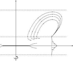
Following Prandtl's hierarchical approach, we introduce an outer region where the flow is inviscid, as well as an inner region corresponding to the boundary layer, and where the viscous terms are comparable with the convective terms. The structure of the flow is sketched in figure 3. In the outer region, denoted region $2$ in figure 3, we have

(2.30a,b)\begin{equation} r,\quad z=O(1). \end{equation}

We will prove afterwards that the flow is indeed inviscid in region $2$ in the limit (2.30a,b).

Figure 3.

Structure of the flow. The part for negative $\hat {r}$ has been omitted. The fluid is stagnant in region $3$. Region $2$ corresponds to the outer inviscid region where the entrainment effect takes place. Region $1$ is the viscous boundary layer. Region $1_{gw}$ is Goldstein's wake immediately downstream of the disk edge, and studied in § 6. Region $1_{ps}$ is the $\textit {Re}^{-1/2}\times \textit {Re}^{-1/2}$ region in the vicinity of the pseudo-shock.

Let us introduce the boundary layer, called region $1$, in the direct neighbourhood of the disk. We define a new scaled variable $Z$ such that in this region

(2.31a,b)\begin{equation} r,\quad Z=\frac{z}{\textit{Re}^{{-}1/2}}=O(1). \end{equation}

The inner expansions that are valid inside the boundary layer have the following form in leading order:

(2.32)\begin{equation} \left.\begin{gathered} u=U(r,Z,t)+\cdots, \\ v=V(r,Z,t)+\cdots, \\ w=\textit{Re}^{{-}1/2}W(r,Z,t)+\cdots, \\ p=\textit{Re}^{{-}1/2}P(r,Z,t)+\cdots, \end{gathered}\right\}\quad \textrm{as}\ \textit{Re}\to\infty. \end{equation}

Substitution of the inner expansions (2.32) into the dimensionless Navier–Stokes equations leads to Prandtl's boundary-layer equations which have been written in conservative form:

(2.33a)\begin{gather} \frac{\partial U}{\partial t}+\frac{\partial (U^2)}{\partial r}+\frac{\partial (UW)}{\partial Z}+\frac{U^2-V^2}{r}=\frac{\partial ^2U}{\partial Z^2}, \end{gather}

(2.33b)\begin{gather}\frac{\partial V}{\partial t}+\frac{\partial (UV)}{\partial r}+\frac{\partial (VW)}{\partial Z}+\frac{2UV}{r}=\frac{\partial ^2V}{\partial Z^2}, \end{gather}

(2.33c)\begin{gather}\frac{\partial P}{\partial Z}=0, \end{gather}

(2.33d)\begin{gather}\frac{\partial U}{\partial r}+\frac{\partial W}{\partial Z}+\frac{U}{r}=0, \end{gather}

(2.33e)\begin{gather}V=r,\ U=W=0, \quad \textrm{at}\ Z=0,\ r \in [0,1], \end{gather}

(2.33f)\begin{gather}\frac{\partial U}{\partial Z}=\frac{\partial V}{\partial Z}=W=0, \quad \textrm{at}\ Z=0,\ r > 1, \end{gather}

(2.33g)\begin{gather}U=V=0, \quad \textrm{at}\ Z=\infty, \end{gather}

(2.33h)\begin{gather}P=\lim_{z\to0}P', \quad \textrm{at}\ Z=\infty, \end{gather}

(2.33i)\begin{gather}U=V=0, \quad \textrm{at}\ r=0, \end{gather}

where the term $\lim _{z\to 0}P'$ in the matching condition for the pressure field corresponds to the inner limit of the leading-order term of the outer expansion for the pressure.

Let us get back to the outer region $2$. Outside the boundary layer $1$ there is a region where there is a slow movement of fluid due to the rotation of the disk as sketched in figure 3. This is referred to as the entrainment effect. The fluid particles are sucked down, and once they reach the boundary layer, they undergo a significant acceleration owing to the action of viscous forces, and they are redirected away from the axis of rotation of the disk. Let us introduce a new scaled independent variable $z'$, such that in region $2$

(2.34)\begin{equation} z'=\frac{z}{\delta'(\textit{Re})}=O(1), \end{equation}

where it is assumed that $\delta '(\textit {Re})\gg \textit {Re}^{-1/2}$. The axial velocity component is comparable in order of magnitude with $\textit {Re}^{-1/2}$ since it is what comes into the boundary layer, and there is a matching for $w$ between regions $1$ and $2$. The asymptotic expansions of the sought flow functions in region $2$ have the following form:

(2.35)\begin{equation} \left.\begin{gathered} u=\sigma'(\textit{Re})U'(r,z',t)+\cdots, \\ v=\eta'(\textit{Re})V'(r,z',t)+\cdots, \\ w=\textit{Re}^{{-}1/2}W'(r,z',t)+\cdots, \\ p=\chi'(\textit{Re})P'(r,z',t)+\cdots, \end{gathered}\right\}\quad \textrm{as}\ \textit{Re}\to\infty, \end{equation}

where $\sigma '$, $\eta '$ and $\chi '$ are to be found. Let us substitute (2.34) and (2.35) into the continuity equation (2.29d). Using the principle of least degeneration yields

(2.36)\begin{equation} \sigma'(\textit{Re})\delta'(\textit{Re})=\textit{Re}^{{-}1/2}. \end{equation}

Following our assumption $\delta '(\textit {Re})\gg \textit {Re}^{-1/2}$, we get

(2.37)\begin{equation} \sigma'(\textit{Re})\ll 1. \end{equation}

Let us substitute (2.35) and (2.34) into the radial momentum equation (2.29a). In the limit as $\textit {Re}\to \infty$ and (2.37), it reduces to

(2.38)\begin{equation} \sigma'(\textit{Re})\frac{\partial U'}{\partial t}-\eta'^2(\textit{Re})\frac{V'^2}{r}={-}\chi'(\textit{Re})\frac{\partial P'}{\partial r}. \end{equation}

We notice that the viscous terms were disregarded. The same applies to the circumferential and axial momentum equations. Thus, the Navier–Stokes equations become the Euler equations, and the flow inside region $2$ may be treated as inviscid.

Let us now prove that the circumferential velocity component is zero in region $2$. We denote by $\varGamma (t)$ the circulation at time $t$ along a closed fluid contour $\mathcal {C}$. The flow in region $2$ is inviscid, incompressible and without any body force acting on the fluid, so according to Kelvin's circulation theorem, the circulation $\varGamma$ along any closed fluid contour $\mathcal {C}$ is invariant with time. Before the disk starts rotating, the fluid is at rest, so the velocity vector $\boldsymbol {V}$ is equal to the zero vector everywhere in the domain. Hence, along any closed fluid contour $\mathcal {C}_0$, the circulation is equal to $0$. According to Kelvin's circulation theorem, the circulation along any closed contour $\mathcal {C}$ will remain equal to $0$ after the disk starts rotating, and, using Stokes theorem, it results that

(2.39)\begin{equation} \oint_{(\mathcal{C})}\boldsymbol{V}\boldsymbol{\cdot}\mathbf{d}\boldsymbol{r}=\iint_{(\sigma)} \boldsymbol{\omega}\boldsymbol{\cdot}\mathbf{d}\boldsymbol{S}=0, \end{equation}

where $\sigma$ is a surface based on $\mathcal {C}$ and $\mathbf {d}\boldsymbol {S}=\boldsymbol {n}\,\textrm {d}S$ is a small element of $\sigma$, with $\boldsymbol {n}$ being a normal unit vector to $\sigma$. Since $\mathcal {C}$ is arbitrary, then we deduce that the flow is irrotational in region $2$:

(2.40)\begin{equation} \boldsymbol{\omega}=0. \end{equation}

Since the flow is irrotational, there exists a scalar function $\varphi$ called the velocity potential, such that

(2.41)\begin{equation} \boldsymbol{V}=\frac{\partial \varphi}{\partial r}\boldsymbol{e}_{\boldsymbol{r}}+\frac{\partial \varphi}{\partial z}\boldsymbol{e}_{\boldsymbol{z}}. \end{equation}

As the flow is axisymmetric, there is no $\boldsymbol {e}_{\boldsymbol {\varPhi }}$ component. Consequently in region $2$, $V'=0$ everywhere. This means that in the leading-order approximation, the circumferential velocity is zero. However, the higher-order terms of the asymptotic expansion of $v$ in (2.35) are not necessarily equal to $0$.

Let us now try to get the solution in region $2$. Since the flow is irrotational, the second component of the vorticity field $\boldsymbol {\omega }$ gives

(2.42)\begin{equation} \frac{\partial u}{\partial z}-\frac{\partial w}{\partial r}=0. \end{equation}

Besides, since the flow is incompressible and axisymmetric, from the continuity equation (2.29d) one can define the dimensionless stream function $\psi$ such that

(2.43a,b)\begin{equation} ru=\frac{\partial \psi}{\partial z},\quad rw={-}\frac{\partial \psi}{\partial r}. \end{equation}

By substituting (2.35) into the second equation in (2.43a,b), we deduce the form of the asymptotic expansion of $\psi$ in region $2$:

(2.44)\begin{equation} \psi=\textit{Re}^{{-}1/2}\psi'+\cdots,\quad \textrm{as}\ \textit{Re}\to\infty. \end{equation}

The substitution of (2.43a,b) into (2.42) yields

(2.45)\begin{equation} \frac{\partial ^2\psi}{\partial r^2}-\frac{1}{r}\frac{\partial \psi}{\partial r}+\frac{\partial ^2\psi}{\partial z^2}=0. \end{equation}

Equation (2.45) can be solved numerically with the right boundary conditions, and the solution $\psi$ will allow us to plot the streamline pattern in region $2$. Substitution of (2.34) and (2.44) into (2.45) leads to

(2.46)\begin{equation} \delta'(\textit{Re})=1, \end{equation}

which means that the thickness of region $2$ is comparable with its length. Consequently, it follows from (2.36) that

(2.47)\begin{equation} \sigma'(\textit{Re})=\textit{Re}^{{-}1/2}. \end{equation}

So the radial velocity component has the same order of magnitude as the axial velocity component. Finally, we balance the local acceleration in the radial momentum equation with the pressure gradient, yielding

(2.48)\begin{equation} \chi'(\textit{Re})=\textit{Re}^{{-}1/2}. \end{equation}

All the asymptotic expansions of the sought flow functions are now known. It is more straightforward to get the solution in region $2$ by solving (2.45), which is the governing equation in region 2 but written in terms of the stream function. Replacing $z'$, and $\psi$ by its asymptotic expansion (2.44), keeping the $O(\textit {Re}^{-1/2})$ terms, the governing equation of region $2$ may be written as follows:

(2.49a)\begin{equation} \frac{\partial ^2\psi'}{\partial r^2}-\frac{1}{r}\frac{\partial \psi'}{\partial r}+\frac{\partial ^2\psi'}{\partial z'^2}=0. \end{equation}

At $z'=0$, the matching condition with the solution from the boundary layer must be satisfied. We recall that $w=O(\textit {Re}^{-1/2})$ inside the boundary layer and in region $2$. Hence, the matching condition for the axial velocity component can be written as

(2.49b)\begin{equation} W'=\lim_{Z\to\infty}{W} \quad \textrm{at}\ z'=0. \end{equation}

Consequently, the matching condition related to $\psi '$ at $z'=0$ has the form

(2.49c)\begin{equation} \lim_{Z\to\infty}{W}={-}\frac{1}{r}\frac{\partial \psi'}{\partial r} \quad \textrm{at}\ z'=0. \end{equation}

On the axis of rotation of the disk, we recall that the radial velocity component is equal to $0$ as the flow is axisymmetric. Consequently

(2.49d)\begin{equation} \psi'=0 \quad \textrm{at}\ r=0. \end{equation}

When $z'$ is large, the solution must match with the stagnant fluid of region $3$. Furthermore, when $r$ is large and positive, the fluid is also at rest since it is located before the front of the pseudo-shock. Even though the velocity components tend to zero when $r$ or $z'$ is large, it would not be correct to set $\psi '=0$ when $r$ or $z'$ is large, since the distances over which we would integrate the velocity in order to obtain $\psi '$ also become large. Instead, we write

(2.49e)\begin{equation} \frac{\partial \psi'}{\partial r}=\frac{\partial \psi'}{\partial z'}=0, \quad \textrm{at}\ r^2+z'^2=\infty. \end{equation}

3. Computational analysis

We solve the boundary-value problem (2.33a)–(2.33i) numerically with the help of the following finite-difference method. We employ a uniform grid $\{r_i,Z_k,t_n\}=\{\Delta r(i-1),\Delta Z(k-1),\Delta t(n-1)\}$ such that $i \in [\![1;N_r+1]\!]$, $k \in [\![1;N_Z+1]\!]$, $n \in [\![1;N_t+1]\!]$, and where $\Delta r$, $\Delta Z$ and $\Delta t$ are small grid spacings in the $r$ direction, the $Z$ direction and for time, respectively. For the time derivatives, a backward Euler scheme is employed:

(3.1a)\begin{equation} \frac{\partial U}{\partial t}=\frac{U^{n}_{i,k}-U^{n-1}_{i,k}}{\Delta t}, \end{equation}

where $U^{n}_{i,k}$ is the approximated value of $U$ at the $(i,k,n)$ node: $U^{n}_{i,k}\approx U(r_i,Z_k,t_n)$. Regarding space derivatives, we use second-order schemes for $\partial /\partial Z$ and $\partial ^2/\partial Z^2$, while a first-order scheme is employed for $\partial /\partial r$. The reason why we choose to use a first-order scheme for $\partial /\partial r$ instead of a second-order one is because of the hyperbolic nature of the operator $\partial U/\partial t+U\partial U/\partial r$. We expect to observe discontinuities of the flow quantities, so the error brought by a second-order scheme would be very large in that case.

Discretisation of the boundary-layer equations (2.33a)–(2.33i) leads to a set of nonlinear algebraic equations for $U^{n}_{i,k}$, $V^{n}_{i,k}$ and $W^{n}_{i,k}$. When solving these equations, we use iterative techniques which rely on linearisation of our equations. In particular, when dealing with $U^2$ in (2.33a), we apply Newton's method which consists of using the Taylor expansion around an approximate value of $U$, denoted by $U^-$, as follows:

(3.1b)\begin{equation} U^2\approx{-}(U^-)^2+2U^-U. \end{equation}

Consequently, the $r$ derivative of $U^2$ can be written

(3.1c)\begin{equation} \frac{\partial (U^2)}{\partial r}=\frac{(U^n_{i,k})^2-(U^n_{i-1,k})^2}{\Delta r}=\frac{2(U^-)^n_{i,k}}{\Delta r}U^n_{i,k}-\frac{((U^-)^n_{i,k})^2+(U^n_{i-1,k})^2}{\Delta r}. \end{equation}

The term $UW$ in (2.33a) may be linearised by decoupling the equations of the system (2.33a)–(2.33i): $UW$ becomes $W^-U$, where $W^-$ is a computed approximation of $W$. Hence, the $Z$ gradient of $UW$ may be written

(3.1d)\begin{align} \frac{\partial (UW)}{\partial Z}&=\frac{U^n_{i,k+{1}/{2}}W^n_{i,k+{1}/{2}}-U^n_{i,k-{1}/{2}}W^n_{i,k-{1}/{2}}}{\Delta Z}\nonumber\\ &=\frac{(W^-)^n_{i,k+1}+(W^-)^n_{i,k}}{4\varDelta Z}U^n_{i,k+1}+\frac{(W^-)^n_{i,k+1}-(W^-)^ n_{i,k-1}}{4\Delta Z}U^n_{i,k} \nonumber\\ &\quad -\frac{(W^-)^n_{i,k}+(W^-)^n_{i,k-1}}{4\Delta Z}U^n_{i,k-1}. \end{align}

The last two terms in (2.33a) are discretised as follows:

(3.1e)\begin{align} \frac{U^2-V^2}{r}&=\frac{(U^n_{i,k})^2-((V^-)^n_{i,k})^2}{r_i} \nonumber\\ &=\frac{2(U^-)^n_{i,k}}{r_i}U^n_{i,k}-\frac{((U^-)^n_{i,k})^2+((V^-)^n_{i,k})^2}{r_i}, \end{align}

(3.1f)\begin{equation} \frac{\partial ^2 U}{\partial Z^2}=\frac{1}{(\Delta Z)^2}U^n_{i,k-1}-\frac{2}{(\Delta Z)^2}U^n_{i,k}+\frac{1}{(\Delta Z)^2}U^n_{i,k+1}. \end{equation}

The circumferential momentum equation (2.33b) is dealt with in a similar way. We use marching methods to solve numerically the boundary-value problem (2.33a)–(2.33i). For a fixed $n$ and computational line $r_i$, we solve sequentially (2.33a), (2.33b) and (2.33d) and we iterate until the absolute residual $\left \lVert \boldsymbol {F}(U,V,W)\right \rVert$ becomes smaller than a small parameter $\varepsilon$, where $\boldsymbol {F}$ is a column vector such that the set of equations (2.33a)–(2.33b) discretised with the numerical schemes presented above can be written as $\boldsymbol {F}=\boldsymbol {0}$. At each iteration, $U$ and $V$ are obtained sequentially by making use of the Thomas algorithm. The axial velocity component is deduced for the current iteration because of the continuity equation (2.33d):

(3.2)\begin{equation} W^n_{i,k}=W^n_{i,k-1}-\Delta Z\left(\frac{(U^-)^n_{i,k}-U^n_{i-1,k}}{\Delta r}+\frac{(U^-)^n_{i,k}}{r_i}\right), \quad \forall k \in [\![2;N_Z+1]\!]. \end{equation}

4. Numerical results

In order to resolve both singularities near the edge of the disk and the pseudo-shock, a rather refined mesh in the $r$ direction was required (see table 1). Then, following the Courant–Friedrichs–Lewy condition and the fact that the tridiagonal matrix used in the Thomas algorithm must be diagonally dominant, the grid spacings $\Delta t$ and $\Delta Z$ must be decreased accordingly. The matching conditions (2.33g) for $U$ and $V$ at $Z=\infty$ turn to Dirichlet boundary conditions computationally speaking. Therefore, the upper limit of the computational domain, denoted as $Z_{max}$, must be large enough to satisfy (2.33g). To ensure that, we pick a $Z_{max}$ when $U$ and $V$ decreased at least to $1\,\%$ of their maximum values. The results of the calculations with the mesh presented in table 1 are displayed in figure 4. For grid convergence details, see the Appendix. The radial velocity $U$ is plotted against $r$ on the jet axis for different values of time $t$. We observe as expected a pseudo-shock propagating as time increases in the positive $r$ direction. It consists of a discontinuity in $U$, such that immediately downstream the flow is at rest. Immediately behind the shock, the velocity is finite and positive. The same features have been observed in the circumferential velocity component $V$, plotted against $r$ on the jet axis and for different values of time. Regarding the axial velocity component, we plotted it at the outer edge of the boundary layer against $r$ for the corresponding times $t$. Starting from $r=0$, $W$ is negative and remains globally constant up to the vicinity of the shock, where it decays slightly before bursting at the position of the shock. Immediately downstream of the shock, it is equal to $0$. The negative sign of $W$ in the main part of the boundary layer confirms the analysis performed in § 2 for the entrainment effect. Our calculations showed that when $\Delta r$ is smaller, the discontinuity of the velocity components is emphasised. This is consistent with the fact that discretising our problem with the finite-difference method introduced a truncation error $O(\Delta t, \Delta r, (\Delta Z)^2)$, so the quotient $\Delta U/\Delta r$ must tend to $-\infty$ at the pseudo-shock's position as the grid spacing $\Delta r$ tends to $0$. A change of $\Delta Z$ did not produce any significant difference. The parameter $Z_{max}$ has been chosen such that it is large enough so that the velocity components $U$ and $V$ are almost $0$ at $Z_{max}$, as discussed earlier.

Figure 4.

The radial, circumferential and axial velocity components plotted against $r$ for different values of $t$. (a) Radial velocity along the jet axis at time $t=4$, 6, 8, 10, 12. (b) Circumferential velocity along the jet axis at time $t=4$, 6, 8, 10, 12. (c) Axial velocity at $Z=Z_{max}$ at time $t=4$, 6, 8, 10, 12.

Table 1.

Mesh parameters.

One last interesting plot is a comparison of our results with the von Kármán flow. Von Kármán (Reference von Kármán1921) solved the Navier–Stokes equations for the case of a disk of infinite radius placed in an infinite region filled with an initially stagnant fluid, and he studied the steady solution. The notation, the coordinate system and the reference frame are the same as those we introduced in the case of the disk with finite radius. Von Kármán sought the solution in the following form:

(4.1a)\begin{equation} \hat{u}=\varOmega\hat{r}F(\zeta),\quad \hat{v}=\varOmega\hat{r}G(\zeta),\quad \hat{w}=\sqrt{\varOmega\nu}H(\zeta), \end{equation}

with the functions $F$, $G$ and $H$ being determined numerically, and where the variable $\zeta$ is defined such that

(4.1b)\begin{equation} \zeta=\sqrt{\frac{\varOmega}{\nu}}\hat{z}. \end{equation}

We wish to compare our unsteady solution for different values of time with the von Kármán steady solution. For obvious reasons, this will be done for $|r|\leqslant 1$. Let us scale the quantities in (4.1a) and (4.1b) so that they can match the variables we observed numerically in the case of a disk of finite radius. We recall that we introduced the dimensionless variable $z$ such that $\hat {z}=Rz$, and that the Reynolds number is defined such that $\textit {Re}=\varOmega R^2/\nu$. Consequently, the variable (4.1b) becomes

(4.2)\begin{equation} \zeta=Z, \end{equation}

where we used the scaled variable $Z=z/\textit {Re}^{-1/2}$. Thus, on the boundary-layer scale, the flow quantities in (4.1a) have the following form:

(4.3a–c)\begin{equation} U=rF(Z),\quad V=rG(Z),\quad W=H(Z). \end{equation}

Now, we can compare our radial and circumferential velocity components with the von Kármán solution by dividing them by $r$. The comparison has been performed for $U$ in figure 5 for two values of time, where we arbitrarily chose $r=0.5$. We can see that our numerical solution at times $t=4$ and $t=6$ is very close to the von Kármán steady solution. Our calculations showed that from $t=10$, we can consider that the steady state is reached (for $|r|\leqslant 1$), and that our solution matches with that of von Kármán.

Figure 5.

Comparison of the von Kármán solution $F$ with $U/r$ at $t=4$ and $t=6$ for $r=0.5$.

We plot in figure 6 the solution of the system (2.49a)–(2.49e) governing the flow in region $2$ at $t=6$. A uniform grid was employed, where the grid spacing in the $z'$ direction is $\Delta z'=0.001$. The upper limit of the domain has been chosen as $z'_{max}=20$. The results of figure 6 show that for the flow in region $2$, the pseudo-shock serves as a point source. It injects the fluid into region $2$ and then this fluid is entrained back into the boundary layer upstream of the pseudo-shock. The point source is located at a different position when the streamline pattern is plotted at another time as the pseudo-shock moves in the positive $r$ direction as time increases.

Figure 6.

Streamline pattern of the flow in region $2$ at $t=6$.

5. Internal structure of the pseudo-shock

The boundary-layer theory formulated by Prandtl (Reference Prandtl1904) is based on the assumption that the longitudinal gradients of the fluid-dynamic functions are small in comparison with those in the transverse direction. Indeed, in our case,

(5.1)\begin{equation} \frac{\partial \hat{u}}{\partial \hat{r}}\ll\frac{\partial \hat{u}}{\partial \hat{z}}, \end{equation}

because $\hat {z}=R\textit {Re}^{-1/2}Z$, with the Reynolds number being large. However, the numerical results showed us that the rotation of the disk generates a pseudo-shock propagating away from the rim of the disk as time increases. This shock consists of a discontinuity in the velocity components such that their derivatives with respect to $r$ tend to infinity as the grid spacing $\Delta r$ tends to $0$. Therefore, the assumption of the smallness of the longitudinal gradients is valid everywhere in the boundary layer, except in a small region in the vicinity of the pseudo-shock where they become equal in order of magnitude to the transverse gradients. The boundary-layer theory is not valid in this region, so we need to predict the form of asymptotic expansions. In this new region, we need to allow the pressure to change across the jet. For this to happen, the length $\Delta \tilde {r}$ of the pseudo-shock should be comparable with the thickness of the jet. Hence,

(5.2)\begin{equation} \Delta\tilde{r}\sim\textit{Re}^{{-}1/2}. \end{equation}

For a detailed discussion of this issue, the reader is referred to Ruban & Vonatsos (Reference Ruban and Vonatsos2008).

Let us notice that the longitudinal extent $\Delta \tilde {r}$ of this pseudo-shock is much larger as compared to the characteristic thickness of shock waves in classical gas dynamics. Indeed, a normal shock consists of a jump in the sought flow functions, and this jump may be smoothed out by observing it at a different scale, allowing the determination of the characteristic thickness of the region in the vicinity of the shock. The thickness of the classical shock in gas dynamics is an $O(\textit {Re}^{-1})$ quantity and it is comparable with the molecular mean free path $\lambda _m$. As a consequence, the continuum hypothesis is not valid for describing the internal structure of this shock. In the case of our pseudo-shock generated by the rotation of the disk, its thickness is much larger than an $O(\textit {Re}^{-1/2})$ quantity. This allows us to use the Navier–Stokes equations when describing its internal structure, and this is why we refer to it as a ‘pseudo’-shock.

We need to introduce a new scaled variable $X$ accordingly to (5.2). Since we want to study the flow behaviour in the vicinity of the moving pseudo-shock, it is convenient to perform our analysis in the reference frame moving with the shock. Based on that and on (5.2), we write

(5.3a,b)\begin{equation} Z,\quad X=\frac{r-r_s(t)}{\textit{Re}^{{-}1/2}},=O(1), \end{equation}

where $r_s(t)$ is the pseudo-shock's position at time $t$. This new $\textit {Re}^{-1/2}\times \textit {Re}^{-1/2}$ region is called $1_{ps}$.

We may write the asymptotic expansions of the fluid-dynamic functions on the pseudo-shock's scale in the reference frame moving with it:

(5.4)\begin{equation} \left.\begin{gathered} u=V_s(t)+\tilde{U}(X,Z,t)+\cdots, \\ v=\tilde{V}(X,Z,t)+\cdots, \\ w=\tilde{W}(X,Z,t)+\cdots, \\ p=\tilde{P}(X,Z,t)+\cdots, \end{gathered}\right\}\quad \textrm{as}\ \textit{Re}\to\infty,\end{equation}

where $V_s(t)$ is the shock speed at time $t$. The reader is referred to Ruban & Vonatsos (Reference Ruban and Vonatsos2008) for detailed explanations about the form of the asymptotic expansions. Substitution of (5.4) into the Navier–Stokes equations shows that the flow in the region in the vicinity of the pseudo-shock is governed by the Euler equations

(5.5a)\begin{gather} \tilde{U}\frac{\partial \tilde{U}}{\partial X}+\tilde{W}\frac{\partial \tilde{U}}{\partial Z}={-}\frac{\partial \tilde{P}}{\partial X}, \end{gather}

(5.5b)\begin{gather}\tilde{U}\frac{\partial \tilde{V}}{\partial X}+\tilde{W}\frac{\partial \tilde{V}}{\partial Z}=0, \end{gather}

(5.5c)\begin{gather}\tilde{U}\frac{\partial \tilde{W}}{\partial X}+\tilde{W}\frac{\partial \tilde{W}}{\partial Z}={-}\frac{\partial \tilde{P}}{\partial Z}, \end{gather}

(5.5d)\begin{gather}\frac{\partial \tilde{U}}{\partial X}+\frac{\partial \tilde{W}}{\partial Z}=0. \end{gather}

Then, in the $\textit {Re}^{-1/2}\times \textit {Re}^{-1/2}$ region, the problem is quasi-steady and quasi-two- dimensional in the leading-order approximation when observed in the reference frame moving with the shock. The system formed by (5.5a), (5.5c) and (5.5d) can be solved independently as a two-dimensional system. Since the flow is two-dimensional and incompressible, one can define the stream function $\tilde {\psi }$ such that

(5.6a,b)\begin{equation} \tilde{U}=\frac{\partial \tilde{\psi}}{\partial Z},\quad \tilde{W}={-}\frac{\partial \tilde{\psi}}{\partial X}. \end{equation}

Since the flow is quasi-steady and dictated by the inviscid flow theory, the Bernoulli equation is applicable:

(5.7)\begin{equation} H(\tilde{\psi})=\tfrac{1}{2}(\tilde{U}^2+\tilde{W}^2)+\tilde{P}, \end{equation}

where the quantity $H(\tilde {\psi })$ is constant along each streamline.

Our task now is to predict theoretically the flow behaviour in the $\textit {Re}^{-1/2}\times \textit {Re}^{-1/2}$ region. We also determine the speed of the shock $V_s(t)$ at time $t$. Immediately behind the shock, the radial velocity component inside the main part of the boundary layer is $U(r^-_s(t),Z,t)$, so the Prandtl matching rule yields

(5.8a)\begin{gather} U(r^-_s(t),Z,t)=V_s(t)+\tilde{U}(-\infty,Z,t), \end{gather}

(5.8b)\begin{gather}0=\tilde{W}(-\infty,Z,t). \end{gather}

In front of the shock, the matching is performed with the stagnant fluid, where the radial velocity component is $U(r^+_s(t),Z,t)$. So the matching with the flow downstream of the shock gives

(5.8c)\begin{gather} 0=V_s(t)+\tilde{U}(\infty,Z,t), \end{gather}

(5.8d)\begin{gather}0=\tilde{W}(\infty,Z,t). \end{gather}

Let us denote by $\tilde {U}_+$ and $\tilde {U}_-$ the radial components of the velocity on the jet axis at $X=-\infty$ and $X=\infty$, respectively. According to matching conditions (5.8a) and (5.8c), we have

(5.9a)\begin{gather} \tilde{U}_+{=}U(r^-_s(t),0,t)-V_s(t), \end{gather}

(5.9b)\begin{gather}\tilde{U}_-{=}-V_s(t). \end{gather}

The inner structure of the pseudo-shock is sketched in figure 7. The matching conditions (5.8c) and (5.8d) show that downstream of the shock, in the reference frame moving with it, there is a uniform stream between $B$ and $C$ with the speed $-V_s(t)$. On the jet axis $DC$, the radial velocity component $\tilde {U}$ varies from a positive value equal to $\tilde {U}_+$ at point $D$ to a negative value at point $C$ equal to $\tilde {U}_-$. Therefore, there must exist a stagnation point $S$ on the jet axis, somewhere between $D$ and $C$. This stagnation point $S$ is due to the collision of the fluid elements coming from $ED$ and those coming from $BC$. We expect to observe a dividing streamline $FS$ and recirculation regions developing in the region delimited by $FSD$. The location of point $F$ in figure 7 corresponds to the point where the stream function $\tilde {\psi }$ is equal to $0$ at $X=-\infty$ and $Z\neq 0$. Indeed, along the jet axis $DC$, the symmetry condition holds:

(5.10)\begin{equation} \frac{\partial \tilde{U}}{\partial Z}=\tilde{W}=0,\quad\textrm{at}\ Z=0. \end{equation}

Consequently, the stream function is equal to $0$ everywhere on the jet axis. At $X=-\infty$, $\tilde {U}$ is positive at $Z=0$ and decreases up to point $E$ where it becomes $0$, and keeps decreasing and tends to $-V_s(t)$ as $Z\to \infty$. Hence, according to this observation, and using the definition of $\tilde {\psi }$ formulated in (5.6a,b), we expect that $\tilde {\psi }$ at $X=-\infty$, which is equal to $0$ at $Z=0$, increases up to point $E$, and starts decreasing from point $E$ as $Z$ increases. Besides, $\tilde {\psi }$ is a continuous function of $Z$; it is monotonically decaying from $E$ to $A$ such that $\tilde {\psi }>0$ at point $E$ and $\tilde {\psi }<0$ at point $A$. So according to the intermediate value theorem, there exists a unique point, denoted $F$, such that $\tilde {\psi }=0$ at $X=-\infty$ between $E$ and $A$. Therefore, at $X=-\infty$, the stream function $\tilde {\psi }$ is equal to $0$ at point $D$ (corresponding to $Z=0$) and at point $F$. Since the stream function is constant along each streamline, then we deduce that the dividing streamline is $FS$.

Figure 7.

Inner structure of the pseudo-shock.

Let us apply the Bernoulli equation (5.7) to the streamline $DS$. At point $D$, the radial velocity is given by (5.9a), while the axial velocity is given by (5.8b). Moreover, we proved earlier that the pressure $P$ is constant and equal to $0$ everywhere in the main part of the boundary layer, so $P_D=0$. The point $S$ is a stagnation point, so the velocity is $0$ by definition. However, the pressure at point $S$, denoted as $P_S$, cannot be $0$. The Bernoulli equation applied to the streamline $DS$ yields

(5.11)\begin{equation} \tfrac{1}{2}\tilde{U}^2_+{=}P_S. \end{equation}

At point $C$, the velocity components are given by (5.8c) and (5.8d). The pressure at point $C$ is equal to $0$, as the fluid is stagnant there. Using the Bernoulli equation on streamline $SC$ leads to a second equation involving $P_S$:

(5.12)\begin{equation} P_S=\tfrac{1}{2}\tilde{U}^2_-. \end{equation}

Combining (5.11) with (5.12), it follows that

(5.13)\begin{equation} \tilde{U}_+{=}\pm\tilde{U}_-. \end{equation}

Keeping in mind the geometry of the flow in figure 7, we have to choose

(5.14)\begin{equation} \tilde{U}_+{=}-\tilde{U}_-. \end{equation}

Replacing $\tilde {U}_+$ and $\tilde {U}_-$ by their definition written in (5.9a) and (5.9b) leads to

(5.15)\begin{equation} V_s(t)=\tfrac{1}{2}U(r_s(t),0,t). \end{equation}

This means that the speed of the shock is equal to half the radial velocity on the jet axis at the position immediately behind of the shock. This result is in close agreement with the experiments of Turner (Reference Turner1962). He studied a plume fluid consisting of a salt solution, which initially is in a roof tank placed on top of a large tank of fresh water. An orifice is placed down the roof tank, and a tap lies near to orifice to preclude the salt solution flowing down. When it is opened, the plume starts to flow to the tank of water, and a jet is generated. Turner's measurements show that the speed of the jet front $V_s(t)$ is

(5.16)\begin{equation} V_s(t)=0.49U(r_s(t),0,t). \end{equation}

Our task now is to solve the system of equations (5.5a), (5.5c) and (5.5d). It is currently written with the primitive-variable formulation. We can turn the system into a more convenient form where the pressure will no longer be explicit because of the so-called stream function vorticity formulation:

(5.17a)\begin{gather} \nu_a\frac{\partial \omega}{\partial t}+\tilde{U}\frac{\partial \omega}{\partial X}+\tilde{W}\frac{\partial \omega}{\partial Z}=\nu_a\left(\frac{\partial ^2\omega}{\partial X^2}+\frac{\partial ^2\omega}{\partial Z^2}\right), \end{gather}

(5.17b)\begin{gather}\frac{\partial \psi}{\partial t}-\frac{\partial ^2\tilde{\psi}}{\partial X^2}-\frac{\partial ^2\tilde{\psi}}{\partial Z^2}=\omega, \end{gather}

(5.17c)\begin{gather}\tilde{U}=\frac{\partial \tilde{\psi}}{\partial Z},\quad \tilde{W}={-}\frac{\partial \tilde{\psi}}{\partial X}, \end{gather}

where we defined the scalar vorticity field $\omega$ such that

(5.17d)\begin{equation} \omega=\frac{\partial \tilde{W}}{\partial X}-\frac{\partial \tilde{U}}{\partial Z}. \end{equation}

The vorticity transport equation (5.17a) has been written in its viscous form for the following reasons: its steady counterpart is a hyperbolic type of partial differential equation, so it may develop discontinuities. Our calculations showed that it was leading to the Kelvin–Helmholtz instability, no matter the numerical techniques used. However, this instability can be suppressed by introducing an artificial viscosity $\nu _a$, making the vorticity transport equation of elliptic type. Obviously, $\nu _a$ must be kept small as the flow is supposed to be inviscid in the leading-order approximation. Furthermore, (5.17a) and (5.17b) are written in their unsteady form. This is because the problem can be solved numerically using the pseudo-transient method which was introduced by Burggraf (Reference Burggraf1966). Later, Mallinson & de Vahl Davis (Reference Mallinson and de Vahl Davis1973) applied the pseudo-transient method to the problem of the buoyancy-driven motion of a viscous incompressible fluid in an enclosure. According to them, one needs to multiply the time derivative $\partial \omega /\partial t$ by the parameter $\nu _a$ as this will affect the adjusting of the development of the transient vorticity $\omega$ and the solution will remain independent of $\nu _a$.

Let us now formulate the boundary conditions for equations (5.17a)–(5.17c). On the jet axis, a symmetry condition holds, so the axial velocity component is equal to $0$: so according to (5.17c), $\psi$ is equal to $0$ as well on the jet axis. Regarding $\omega$, a soft boundary condition was chosen:

(5.17e)\begin{equation} \psi=\frac{\partial \omega}{\partial Z}=0, \quad \textrm{at}\ Z=0. \end{equation}

Far from the jet axis, the solution matches with the external inviscid flow, which appears to be uniform in the reference frame moving with the shock, such that the radial velocity component satisfies $\tilde {U}|_{Z=\infty }=-V_s(t)$. Hence, by substituting $\tilde {U}|_{Z=\infty }$ into the first equation in (5.17c) and also into (5.17d), we get

(5.17f)\begin{equation} \frac{\partial \psi}{\partial Z}={-}V_s(t),\ \omega=0, \quad \textrm{at}\ Z=\infty. \end{equation}

At $X=-\infty$, the solution matches with the one immediately behind the pseudo-shock. Since the matching is performed in the reference frame moving with the shock, it is convenient to introduce the function $U_I$ such that

(5.17g)\begin{equation} U_I(Z,t)=U(r_s(t),Z,t)-V_s(t). \end{equation}

Thus, the boundary conditions at $X=-\infty$ may be written as

(5.17h)\begin{equation} \psi=\int_0^Z{U_I(Z,t)\,\textrm{d}Z},\ \omega={-}\frac{\partial U_I}{\partial Z}, \quad \textrm{at}\ X={-}\infty. \end{equation}

In the first equation of (5.17h), the constant of integration has been set equal to $0$ because $\psi =0$ at $Z=0$ according to the boundary condition (5.17e). In the second equation of (5.17h), the term $\partial \tilde {W}/\partial X$ at $X=-\infty$ has been omitted for the following reason: in the main part of the boundary layer, outside of the region of the pseudo-shock, the axial component of the velocity is similar in order of magnitude to $\textit {Re}^{-1/2}$, contrary to the radial component which is of order one. Consequently, since we are working in the limit as $\textit {Re}\to \infty$, the term $\partial \tilde {W}/\partial X$ is negligible as compared to $\partial \tilde {U}/\partial Z$ at $X=-\infty$.

At $X=\infty$, the flow is uniform, so we deduce that

(5.17i)\begin{equation} \psi={-}V_s(t)Z,\ \omega=0, \quad \textrm{at}\ X=\infty. \end{equation}

The set of equations (5.17a)–(5.17c) is discretised by approximating the derivatives with finite differences. We employed a uniform grid $\{X_i,Z_k,t_n\}=\{-X_{max}+\Delta X(i-1),\Delta Z(k-1),\Delta t(n-1)\}$ such that $i \in [\![1;N_X+1]\!]$, $k \in [\![1;N_Z+1]\!]$, $n \in [\![1;\widetilde {N_t}]\!]$, and where $\Delta X$, $\Delta Z$ and $\Delta t$ are small grid spacings in the $X$ direction, the $Z$ direction and for time, respectively. Regarding the left and right limits of the domain, we performed our calculations between $-X_{max}$ and $X_{max}$, where we set $X_{max}$ positive. The number of time steps $\widetilde {N_t}$ is chosen large enough for the steady state to be achieved. This is carried out by monitoring the maximum of the absolute values of both solution changes: the steady state is reached when $\max _{i,k}{|\omega ^{n+1}_{i,k}-\omega ^{n}_{i,k}|}$ and $\max _{i,k}{|\psi ^{n+1}_{i,k}-\psi ^{n}_{i,k}|}$ both become smaller than a small parameter $\varepsilon$. Since our problem is two-dimensional, we use the alternating direction implicit method, which was introduced by Peaceman & Rachford (Reference Peaceman and Rachford1955) in its original form, and later it was formulated in its generalised form by Douglas & Gunn (Reference Douglas and Gunn1964).

We plot the streamlines on the pseudo-shock's scale at $t=8$ in figure 8. The pseudo-shock's position $r_s(t=8)$ is equal to $1.749$, and its speed has been determined numerically, and we found that it is equal to $0.1$ at $t=8$. Furthermore, even though the governing equations are quasi-steady in the leading-order approximation, we had to plot the streamline pattern at a specific time ($t=8$ here) because the initial velocity profile $U_I$ imposed by the matching condition at $X=-\infty$ as well as the shock speed $V_s(t)$ both depend on time. We recall that $U_I$ is given by (5.17g), so here it is written as

(5.18)\begin{equation} U_I(Z,t=8)=U(r=1.749,Z,t=8)-0.1,\quad \textrm{for all}\ Z\geqslant0. \end{equation}

The mesh used to plot figure 8 is presented in table 2. The upper limit of the domain $Z_{max}$ as well as the grid spacing in the $Z$ direction remain the same as in the solution of the boundary-layer equations we obtained in § 4. In figure 8, we can see as expected that there is a dividing streamline along which the stream function is equal to $0$. A recirculation region is observed below this dividing streamline. In the jet region, the streamlines have been plotted for $\psi =0.05$ and $\psi =0.1$. The rest of the streamlines (that is, apart from the area of the recirculation region and the dividing streamline) correspond to $\psi =-0.05$, and $\psi$ between $-0.1$ and $-1.7$, with the interval $\Delta \psi =-0.1$ between each streamline. The choice of the time step $\Delta t$ is important for the convergence of the pseudo-transient method: a smaller $\Delta t$ implies a slower convergence, but also a larger radius of convergence and a better accuracy. In particular, regarding the artificial viscosity $\nu _a$, we were able to set it equal to $0.001$ without any problem of convergence, even with a coarse grid $\Delta t=0.1$ and $\Delta X=0.1$. However, when we kept decreasing it further, the solution change started to oscillate and our computer code did not converge. One way to remedy this issue is to decrease our parameter $\Delta t$. Thus, we managed to get a stable and convergent solution with a small artificial viscosity $\nu _a=0.0001$ when $\Delta t=0.01$. A smaller artificial viscosity implies that the tangent to the dividing streamline at the stagnation point is more vertical, which is what we expect to see at the stagnation point. A change in the grid spacing $\Delta X$ did not produce any significant variation in the streamline pattern.

Figure 8.

Streamline pattern of the flow on the pseudo-shock's scale at $t=8$.

Table 2.

Mesh parameters used to solve the discretised governing equations in the $\textit {Re}^{-1/2}\times \textit {Re}^{-1/2}$ region in the vicinity of the pseudo-shock.

6. Goldstein's wake

Here our goal is to study the flow in the vicinity of $r=1^+$ and to determine the asymptotic expansions of the sought flow functions. Let us set the variable $s$ such that

(6.1)\begin{equation} s=r-1. \end{equation}

The flow in region $1$ is governed by the boundary-layer equations (2.33a)–(2.33i). For $|r|\leqslant 1$, the no-slip condition (2.33e) must be satisfied on the disk surface: in particular, the radial velocity must be equal to $0$. The solution of the boundary-layer equations with which we are dealing is sought in the class of continuous functions with respect to $r$:

(6.2)\begin{equation} U(r,Z,t)=U_0(Z,t)+o(1), \quad \textrm{as}\ s\to0^+ , \end{equation}

where $U_0(Z,t)$ behaves near the disk surface as follows:

(6.3)\begin{equation} U_0(Z,t)=\lambda_1 Z+O(Z^2), \quad \textrm{as}\ Z\to0, \end{equation}

with $\lambda _1=\partial U_0/\partial Z|_{Z=0}$ being the dimensionless radial skin friction on the disk surface. Immediately downstream of the edge of the disk at $r=1^+$, the deficit of the velocity near $Z=0$ cannot cease to exist once the fluid leaves the edge of the disk. Hence, as we saw with our numerical results presented in § 4, the boundary layer still exists for $r>1$ and it is still governed by the boundary-layer equations, meaning that (6.2) and (6.3) are still valid. However, (6.3) does not satisfy the symmetry condition (2.33f) which must hold in the wake at $Z=0$. Thus, we are dealing with a singular perturbation problem, so one must introduce a viscous sublayer whose thickness becomes smaller as $s$ tends to $0$. Such a sublayer was first introduced by Goldstein (Reference Goldstein1930) in his analysis of the wake downstream the trailing edge of a flat plate. Let us determine the thickness of this new region that we shall call from now on region $1_{gw}$. Since the flow is viscous, we must balance the convective and viscous terms of the momentum equations: from the radial momentum equation (2.33a) we have

(6.4)\begin{equation} U\frac{\partial U}{\partial r}\sim\frac{\partial ^2U}{\partial Z^2}. \end{equation}

The term $U$ is comparable with $Z$ according to (6.3); therefore the thickness of the viscous sublayer in the wake is estimated as

(6.5)\begin{equation} Z\sim s^{1/3}. \end{equation}

Correspondingly, we introduce a new scaled variable $\zeta$ such that in region $1_{gw}$

(6.6)\begin{equation} \zeta=\frac{Z}{s^{1/3}}=O(1), \quad \textrm{as}\ s\to0^+. \end{equation}

Inside the boundary layer, the stream function $\psi$ is defined by

(6.7a,b)\begin{equation} rU=\frac{\partial \psi}{\partial Z},\quad rW={-}\frac{\partial \psi}{\partial r}. \end{equation}

Using the first definition in (6.7a,b), and knowing that $U\sim Z$, it results that in region $1_{gw}$

(6.8)\begin{equation} \psi\sim s^{2/3}. \end{equation}

This suggests that the asymptotic expansion of the stream function in region $1_{gw}$ has the following form:

(6.9)\begin{equation} \psi=s^{2/3}f_0(\zeta,t)+\cdots, \quad \textrm{as}\ s\to0^+, \end{equation}

where we introduced a function $f_0$ that we determine later. Substitution of (6.9) into (6.7a,b) leads to the asymptotic expansions of the radial and axial velocity components in region $1_{gw}$:

(6.10)\begin{equation} \left.\begin{gathered} U=s^{1/3}\frac{\partial f_0}{\partial \zeta}+\cdots, \\ W=\frac{1}{3}s^{{-}1/3}\left(\zeta\frac{\partial f_0}{\partial \zeta}-2f_0\right)+\cdots, \end{gathered}\right\}\quad \textrm{as}\ s\to0^+. \end{equation}

Our numerical results appear to be well in line with Goldstein's wake singularity (6.10).

It remains to find the asymptotic expansion of the circumferential velocity component. The equation governing $V$ is parabolic, so it also does not allow for discontinuities in $r$. Since $V$ remains smooth in $Z$, we can use a Taylor series expansion about $Z=0$ such that

(6.11)\begin{equation} V=1+\lambda_2 Z+O(Z^2) \quad \textrm{as}\ Z\to0, \end{equation}

where $\lambda _2=\partial V/\partial Z|_{Z=0}$. Thus, $V\sim 1$, and we may guess its asymptotic expansion in region $1_{gw}$ as

(6.12)\begin{equation} V=f_1(\zeta,t)+s^{1/3}f_2(\zeta,t)+\cdots, \quad \textrm{as}\ s\to0^+, \end{equation}

where $f_1$ and $f_2$ are order-one functions. Substitution of (6.10) and (6.12) into the boundary-layer equations yields the following system in the unknowns $f_0$ and $f_1$:

(6.13a)\begin{gather} \frac{\partial ^3 f_0}{\partial \zeta^3}+\frac{2}{3}f_0\frac{\partial ^2f_0}{\partial \zeta^2}-\frac{1}{3}\left(\frac{\partial f_0}{\partial \zeta}\right)^2=0, \end{gather}

(6.13b)\begin{gather}\frac{\partial ^2f_1}{\partial \zeta^2}+\frac{2}{3}f_0\frac{\partial f_1}{\partial \zeta}=0, \end{gather}

(6.13c)\begin{gather}\frac{\partial ^2f_0}{\partial \zeta^2}=\frac{\partial f_1}{\partial \zeta}=f_0=0, \quad \textrm{at}\ \zeta=0, \end{gather}

(6.13d)\begin{gather}\frac{\partial f_0}{\partial \zeta}=\lambda_1 \zeta+\cdots, \quad \textrm{as}\ \zeta\to\infty, \end{gather}

(6.13e)\begin{gather}f_1=1+\cdots, \quad \textrm{as}\ \zeta\to\infty. \end{gather}

Since there are no derivatives with respect to time, the flow near the disk rim is quasi-steady. It is also quasi-two-dimensional according to (6.10) in the limit as $s\to 0^+$. Equation (6.13a) involves only one unknown function $f_0$, so it may be solved independently of (6.13b). We can use shooting methods to solve (6.13a). We set $u_1=f_0$, $u_2=\partial f_0/\partial \zeta$ and $u_3=\partial ^2 f_0/\partial \zeta ^2$. The boundary condition $u_2=\lambda _1\zeta +\cdots$ as $\zeta \to \infty$ has been omitted and replaced by $u_2|_{\zeta =0}=1$, where $1$ has been chosen arbitrarily. It will be shown that once the unknowns $u_1$, $u_2$ and $u_3$ will have been determined in all the domain, no matter the value assigned to $u_2|_{\zeta =0}$, by making use of affine transformations, the boundary condition for $u_2$ at $\zeta =\infty$ can be satisfied. We used finite-difference methods to solve the equations numerically, such that the method is explicit. The numerical results are displayed in figure 9. We used a grid spacing $\Delta \zeta =0.001$, and we plotted the solution for $\zeta \in [0;\zeta _{max}]$. Thus, we found the solution for $f_0$ (let us denote it $\bar {f}_0$), with the modified boundary condition $u_2=1$ at $\zeta =0$. Let us perform affine transformations:

(6.14a,b)\begin{equation} f_0=A\bar{f}_0,\quad \zeta=B\bar{\zeta}. \end{equation}

It is easily seen that (6.13a) remains unchanged if

(6.15)\begin{equation} B=\frac{1}{A}, \end{equation}

where $A$ is arbitrary. Now, we need to satisfy the boundary condition for $u_2$ when $\zeta$ is large. By making use of (6.15), we notice that

(6.16)\begin{equation} \frac{\partial ^2f_0}{\partial \zeta^2}=A^3\frac{\partial ^2\bar{f}_0}{\partial \bar{\zeta}^2}. \end{equation}

Setting $\zeta _{max}$ in the above equation, we see that the constant $A$ can be found from

(6.17)\begin{equation} A^3\left.\frac{\partial ^2\bar{f}_0}{\partial \bar{\zeta}^2}\right|_{\zeta=\zeta_{max}}=\lambda_1. \end{equation}

Setting constant $A$ in this way, the boundary condition for $u_2$ when $\zeta$ is large can be satisfied.

Figure 9.

Solutions $u_1$ and $u_2$.

Let us now focus on equation (6.13b) which can be solved analytically. Let us set $F_1=\partial f_1/\partial \zeta$, then (6.13b) can be rewritten as

(6.18a)\begin{equation} \frac{\partial F_1}{\partial \zeta}+\frac{2}{3}f_0F_1=0. \end{equation}

We assign to it the boundary condition (6.13c):

(6.18b)\begin{equation} F_1=0 \quad \textrm{at}\ \zeta=0. \end{equation}

The general solution of (6.18a) has the form

(6.19)\begin{equation} F_1=C(t)\exp\left({-\tfrac{2}{3}\int_0^\zeta{f_0(\eta)\,\textrm{d}\eta}}\right), \end{equation}

where $C(t)$ is a function depending on $t$. With the boundary condition (6.18b) taken into account, we deduce that $C(t)=0$ for all $t$; hence $F_1=0$ for all $\zeta$ and $t$. Consequently, by making use of the matching condition (6.13e), we find that

(6.20)\begin{equation} f_1=1 \quad \forall\zeta. \end{equation}