


[Election] data needed doctoring to avoid embarrassing situations, as occurred in Oaxaca when a zealous, prospective candidate for office wanted to impress the government officials and mobilized 140 percent of those registered.
A “high government source” inside the PRI PresidencyFootnote 1
And I admitted. . .that we rigged the election. . .I gave the order to change it from 93% to around 80%. . .Because more than 90, just psychologically, that is not well received.
Alexander Lukashenko about the 2006
presidential election in BelarusFootnote 2
INTRODUCTION
“You may have won the election, but I won the count!” was Anastasio Somoza’s rebuke to an opponent who accused him of rigging an election.Footnote 3 A burgeoning literature depicts the many ways in which incumbents attempt to “win the count” and conducts increasingly sophisticated analyses of their detection and deterrence.Footnote 4 Yet while “winning the count” may be directed and facilitated from above, its execution is primarily local. The most frequent forms of electoral fraud—ballot box stuffing, multiple voting, voter intimidation, or the falsification of counts—are ultimately executed at the level of individual polling stations, not by the incumbent but rather a machinery that typically consists of hundreds of political operatives, party members, and state employees.Footnote 5
In spite of rich descriptive accounts of such local-level fraud in qualitative and historical literature, most formal and analytical research on electoral fraud treats its political organization and execution as unproblematic. The incumbent’s machinery of manipulation is assumed to operate as a unified political actor, under the incumbent’s perfect political control. This approach leaves us with a number of puzzles: How does the incumbent ensure that his local agents deliver fraud precisely when needed and exactly as much as is needed? What motivates local agents to engage in fraud when doing so may result in criminal prosecution? Why does locally conducted electoral fraud succeed in delivering a victory in some elections but fail in others?
In this article, we study these puzzles and demonstrate that incentive conflicts in the political organization and execution of electoral fraud have far-reaching implications for its conduct, success, and empirical fingerprints. Two related but distinct incentive conflicts critically shape the political organization of electoral fraud: the principal-agent problem between an incumbent and his local agents, and the collective action problem among the agents.
At the heart of the principal-agent problem is a conflict of interest between the incumbent and his agents about when to engage in fraud and how much of it to conduct. The incumbent’s preferences were eloquently summarized in John F. Kennedy’s facetious response to questions about the role of his father’s wealth in his political success: “I have just received the following wire from my generous daddy. It says, ‘Dear Jack, don’t buy a single vote more than is necessary. I’ll be damned if I’m going to pay for a landslide!’”Footnote 6 That is, even those incumbents who are willing to engage in fraud if it is needed for a victory want to avoid unnecessary fraud that will only raise suspicions. Most agents, meanwhile, prefer to conduct fraud when it carries the least risk—when the incumbent’s victory is assured and the agents’ actions are unlikely to be investigated. Agents are most reluctant to engage in fraud when the incumbent’s victory is in doubt and they worry about being prosecuted if the challenger were to win the election. Put differently, agents are least willing to engage in fraud precisely when incumbents need fraud the most!
This principal-agent problem between the incumbent and his agents is compounded by a collective action problem among the agents. It is most pronounced when the incumbent narrowly trails the challenger. In these scenarios, the incumbent’s agents understand that, if only enough of them engaged in fraud, they could secure the incumbent’s victory. At the same time, however, each agent’s doubts about other agents’ actions lead her to question the prudence of her own engagement in fraud. Hence even when fraud could secure the incumbent’s victory, the agents’ fear of its ultimate failure may turn it into a self-fulfilling prophecy.
In order to rigorously examine the interplay between principal-agent and collective action problems in the political organization and execution of electoral fraud, we develop a formal model with two key, novel features. First, the incumbent does not engage in fraud directly but instead depends on the illicit collaboration of a large number of local agents who must be motivated by the promise of a reward. This is a departure from existing formal research, where the incumbent’s machinery of fraud is assumed to act as a unitary actor.Footnote 7 A key aspect of this departure concerns the contingency of the agents’ reward—as well as their punishment—on the incumbent’s political survival: Each agent understands that, if she engages in fraud, she will obtain the promised reward only if the incumbent is re-elected and may face prosecution if the incumbent is ultimately defeated.Footnote 8
The second key feature of our formalization concerns the limited information available to the incumbent and his local agents when they are deciding whether to engage in fraud. The difficulties that incumbents in hybrid regimes face when gauging their genuine popularity have been highlighted in research on electoral manipulation and democratization (Gehlbach and Simpser Reference Gehlbach and Simpser2015; Little Reference Little2013; Miller Reference MillerForthcoming; Rozenas Reference Rozenas2013) and parallel classic accounts of incentives for “preference falsification” under authoritarianism (Kuran Reference Kuran1991; Wintrobe Reference Wintrobe1998). The novel feature of our model is in how the structure of this information paucity is tailored to the context of electoral manipulation: While both the incumbent and his local agents have only imperfect information about the incumbent’s genuine popularity, each local agent’s information is much more precise than the incumbent’s but at the same time confined to her own precinct.
The chief macropolitical consequence of these two novel features is a herd dynamic among the agents that tends to result in either overwhelming victories for the incumbent or, less often, his resounding defeats. We obtain this prediction by a natural application of the global game approach to the analysis of collective action problems (Carlsson and van Damme Reference Carlsson and van Damme1993; Morris and Shin Reference Morris, Shin, Dewatripont, Hansen and Turnovsky2003).Footnote 9 Its key advantage is to transform a setting that would otherwise suffer from a multiplicity of equilibria with contradictory predictions into one with a unique, tractable, and politically intuitive equilibrium. In our setting, the agents’ incentives result in a unique tipping-point equilibrium according to which an agent engages in fraud only if her local, private perception of the incumbent’s popularity exceeds a threshold. The intuition is as follows: The higher the incumbent’s genuine popularity in an agent’s precinct, the more popular she infers the incumbent to be nationwide; consequently, she anticipates that fewer agents need to engage in fraud in order to secure the incumbent’s victory, which in turn lowers her own risk of engaging in fraud. Thus while never observed perfectly by either the incumbent or the agents, the incumbent’s genuine nationwide popularity ends up playing a central role by tacitly coordinating the agents’ attempts to resolve their collective action problem.
The perverse consequence of such individual-level incentives is a herd dynamic at the aggregate level. Jointly, agents will tend to either oversupply or undersupply fraud, rarely delivering the amount of fraud that would be optimal from the incumbent’s point of view. At one extreme, when the incumbent is unpopular and therefore needs fraud the most, agents will tend to underdeliver it; at the other extreme, agents will deliver excess fraud when it is not needed at all. Put simply, the incumbent cannot order 51% of the vote and expect to get precisely that. The aggregate amount of fraud will approximate the desired level only when he narrowly trails the challenger. It is only in such elections that fraud will be both politically decisive for the incumbent’s victory and successful in securing it.
Our analysis of microincentives in the political organization of electoral fraud improves our understanding of the resulting macrobehavior in a number of ways. First, the equilibrium dynamic that we just described helps us to account for the puzzling, often contradictory accounts of incumbents who enjoy genuine popularity and at the same time engage in seemingly unnecessary fraud. In a seminal analysis of the Institutional Revolutionary Party’s (PRI’s) demise in Mexico, Magaloni (Reference Magaloni2006) observes that, while certainly present, fraud only served to embellish the already impressive popularity that the PRI enjoyed before the 1980s (see also Greene Reference Greene2007; Simpser Reference Simpser2013). Similarly, students of contemporary Russia are puzzled by the embarrassingly obvious fingerprints of fraud in elections that the United Russia party, and especially Vladimir Putin and Dmitry Medvedev, could have won cleanly.Footnote 10 According to a leading explanation for these perplexing outcomes, inflated margins of victory serve to signal the incumbent’s invincibility and thus deter potential challengers or defectors (Magaloni Reference Magaloni2006; Simpser Reference Simpser2013).
Our framework suggests an alternative mechanism: Rather than an intentional strategy, overwhelming incumbent victories are the unintended byproduct of the principal-agent and collective action problems in the political organization of electoral fraud. Because individual agents are most willing to conduct fraud when it carries the least risk—when the incumbent is genuinely popular—we should not be surprised to observe genuine popularity go hand in hand with excessive fraud at the aggregate level.
But this intuition provides only a partial answer to the question of why popular incumbents engage in fraud. If they anticipate an oversupply of fraud, why do popular incumbents allow for fraud in the first place? This is an issue that we address in an extension of our model and the brief answer is: it’s insurance. That is, even those incumbents who expect to prevail generally find it optimal to promise their agents positive (even if small) rewards and thus motivate some fraud, hedging against the odds that they are being too optimistic about their own popularity. As the quotations from PRI-era Mexico and present-day Belarus in our epigraph illustrate, one price that incumbents pay for this insurance is that they get too much fraud when they prove to be right about their popularity. An active infrastructure of fraud thus serves not only those incumbents who cannot win a clean election, but also those who can yet want to insure against an unlikely defeat.
The same logic helps us understand why local-level fraud, even when encouraged by the incumbent, sometimes fails to secure his re-election. Because fraud is by definition illegal, the incumbent’s capacity to motivate agents to engage in fraud on his behalf is limited to the promise of a reward upon his re-election. Such politically contingent inducements, however, are least effective precisely when the incumbent needs the agents’ collaboration most—when he lacks genuine popularity. Our analysis of the ensuing collective action problem highlights how individual agents’ worries about the incumbent’s eventual defeat reverberate among them and, if sufficiently pronounced, multiply into an avalanche of defections from the incumbent. When the incumbent looks like a loser, agents’ fears of the incumbent’s eventual defeat become a self-fulfilling prophecy.
This reasoning suggests a mechanism of fraud deterrence that has not been explored by existing theoretical research but is implicit in recent empirical work. Extant analytical treatments of electoral fraud focus on the threat of a post-election protest or violence as the chief deterrent against fraud (Chernykh and Svolik Reference Chernykh and Svolik2015; Fearon Reference Fearon2011; Little Reference Little2012; Przeworski Reference Przeworski2011; Tucker Reference Tucker2007). By contrast, our arguments highlight that a major reason for the failure of fraud may be the incumbent’s inability to muster the machinery of fraud in the face of his declining popularity.Footnote 11 This focus on the incentives faced by local-level agents parallels empirical research on election monitoring, the deterrent effect of which is also hypothesized to occur at the level of individual polling stations (Asuka et al. Reference Asuka, Brierley, Golden, Kramon and Ofosu2014; Hyde Reference Hyde2008; Ichino and Schüdeln Reference Ichino and Schüdeln2012). Our results, however, suggest that the direct effect of such local-level deterrents—whereby they raise the risk of engaging in fraud for individual agents who are being monitored—may not be the only or even the most consequential one.Footnote 12 Rather, the primary consequence of election monitoring may be indirect: when monitoring occurs, all agents anticipate that much greater efforts must be exerted at nonmonitored polling stations in order to secure the incumbent’s victory, which in turn heightens the collective action dilemma among all agents, including those who are not being monitored. To our knowledge, such systemic consequences of local fraud deterrents have not yet been examined either empirically or theoretically.
An improved understanding of the microincentives faced by the agents who ultimately execute fraud also helps us anticipate its empirical fingerprints. The prevailing approach to fraud detection focuses on the identification of statistical anomalies in voting or turnout but is often less explicit about the political process that generates them.Footnote 13 Our model clarifies that anomalies indicative of fraud may be the unintended consequence of incentive conflicts in the political organization of fraud and predicts a specific pattern that such anomalies should follow: Their occurrence across precincts should not be uniform but rather increasing in both the incumbent’s genuine popularity and his vote share. Yet at the same time, such anomalies alone do not imply that the incumbent stole an election that would have otherwise been won by the challenger. In fact, the fingerprints of fraud may be most pronounced precisely when fraud is not politically decisive.
We find preliminary empirical support for our arguments when we examine the pattern of fraud in the 2011 legislative and 2012 presidential elections in Russia. We confirm a finding from earlier analyses of these elections (Gehlbach Reference Gehlbach2012; Klimek et al. Reference Klimek, Yegorov, Hanel and Thurner2012; Kobak, Shpilkin, and Pshenichnikov Reference Kobak, Shpilkin and Pshenichnikov2012; Mebane Reference Mebane2013), according to which one form of electoral manipulation involved the rounding of the incumbent Vladimir Putin’s and United Russia Party’s vote shares to a higher multiple of 5 by the regime’s local operatives. Crucially, we also identify a previously unnoticed pattern that is anticipated by our model: The extent of such anomalies is increasing in the incumbent’s precinct-level vote share. In order to quantify the extent of fraud, we develop a measure of the ruggedness in the distribution of Putin’s and United Russia’s results based on kernel density estimation and perturbation techniques. Using these two different benchmarks, we find that the distribution of Putin’s and United Russia’s results is too rugged at percentages corresponding to multiples of 5 to occur by chance. Crucially, this ruggedness is indeed increasing in Putin’s and United Russia’s precinct-level vote share, as predicted by our theoretical arguments. Overall, this case illustrates that Putin’s regime used fraud as insurance against an (arguably) unlikely defeat—with its oversupply as the undesirable byproduct of the principal-agent and collective action problems in the political organization of electoral fraud.
THE MODEL
Consider the following electoral manipulation game between an incumbent and his agents.Footnote 14 Each agent i operates in one among a continuum of precincts of equal size and decides whether to engage in fraud on behalf of the incumbent at the time of the election. We denote agent i’s engagement or not in fraud by ai = {f, n}, respectively. The incumbent, however, does not observe whether any agent engaged in fraud; he only observes the precinct-level election result Ri —his share of the vote in agent i’s precinct. Before the election, therefore, the incumbent promises each agent a reward (a higher salary, promotion, perks) commensurate with the election result in her precinct. More precisely, each agent obtains the payoff wRi after the incumbent’s victory, where w ⩾ 0 and we refer to it as the reward factor.
The precinct-level election result Ri depends on the incumbent’s genuine precinct-level popularity Si and whether the agent engaged in fraud on behalf of the incumbent, ai = {f, n}, as follows:Footnote 15
 $$\begin{equation*}
R_i = \left\lbrace \begin{array}{l@{\hspace*{8pt}}l}S_i + F & \text{if $a_i=f$;}\\
S_i & \text{if $a_i=n$.} \end{array} \right.
\end{equation*}$$
Above, the parameter F,
 $0<F<\overline{F}$
, denotes the share of the precinct-level election result due to the agent’s fraud and we interpret it as a measure of the precinct agents’ fraud capacity.Footnote
16
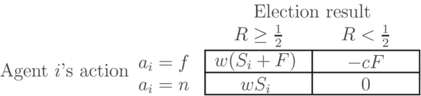
Crucially, the agents obtain the reward wRi only if the incumbent is re-elected. By contrast, if the incumbent loses, each agent’s payoff depends on whether she engaged in fraud at the time of the election. If she did not engage in fraud, she obtains the payoff 0. If she did engage in fraud, the agent obtains the payoff − cF, where c > 0 stands for the political cost of fraud. It reflects the potential investigation of allegations of fraud in the agent’s precinct after the challenger takes office, possibly resulting in the agent’s criminal prosecution and conviction. Thus we are effectively assuming that the likelihood of a conviction or the severity of punishment is increasing in F, the share of the precinct-level election result due to the agent’s fraud.
The agents’ payoffs are summarized in Figure 1. We see that each agent’s incentive to engage in fraud depends on her expectation about the national-level election result R. If the agent expects the incumbent to win,
 $R\ge \frac{1}{2}$
, then she prefers to conduct fraud since w(Si
+ F) > wSi
$for$w > 0.Footnote
17
If, on the other hand, the agent expects the incumbent to lose,
 $R < \frac{1}{2}$
, then she prefers to refrain from fraud since − cF < 0.
Agent i’s Payoffs as a Function of her Fraud Decision ai and the Election Result R

The overall election result R depends on both the incumbent’s genuine popularity and the actions of the agents. More specifically, the incumbent’s popularity at the time of the election θ, 0 < θ < 1, corresponds to the fraction of the electorate that actually voted for the incumbent. We assume that θ is commonly believed to be uniformly distributed on the unit interval (0, 1) but is not perfectly known by any of the players. Instead, each agent privately observes the fraction Si
of her precinct that voted for the incumbent, which is correlated with θ in the following way: Si
is uniformly distributed on the interval (θ − ε, θ + ε),
 $0<\epsilon <\overline{\epsilon }$
.Footnote
18
We think of ε as “small” and interpret it as a measure of heterogeneity in the incumbent’s support across precincts.Footnote
19
Thus when each agent decides whether to engage in fraud on behalf of the incumbent, she has only imperfect information about the incumbent’s genuine, national-level popularity.Footnote
20
Because we model the incumbent’s agents as atomless players along a continuum of precincts, any single agent’s decision to engage in fraud on behalf of the incumbent will be inconsequential at the national level. Jointly, however, the agents’ actions affect the outcome as the overall election result R amounts to
 $$\begin{equation}
R = \int _{\theta -\epsilon }^{\theta +\epsilon } \frac{1}{2 \epsilon } \left( S_i + {\bf 1}_{\lbrace a_i=f\rbrace } F \right) \,d S_i = \theta + \phi F.
\end{equation}$$
Above, 1 {ai = f} is an indicator function that equals 1 if agent i engaged in fraud and 0 otherwise, and ϕ is the fraction of agents that engaged in fraud. We think of our assumption of atomless agents along a continuum of equally sized precincts as capturing a country with a large number of precincts that are small relative to the country as a whole.Footnote 21
The national-level election outcome R thus depends on the precinct agents’ fraud capacity F, the fraction of agents engaging in fraud ϕ, and the incumbent’s election-day popularity θ. If
 $\theta \ge \frac{1}{2}$
, then
 $R\ge \frac{1}{2}$
and the incumbent wins the election regardless of the agents’ actions. If
 $\theta < \frac{1}{2}-F$
, on the other hand, then the incumbent will be defeated even if all agents conducted fraud on his behalf,
 $R < \frac{1}{2}$
. Only when
 $\frac{1}{2}-F \le \theta < \frac{1}{2}$
does the election outcome depend on the fraction of agents ϕ engaging in fraud. In turn, if the agents were able to observe θ perfectly, they would all refrain from fraud when
 $\theta < \frac{1}{2}-F$
, engage in fraud if
 $\theta \ge \frac{1}{2}$
, and condition their actions on the actions of others when
 $\frac{1}{2}-F \le \theta < \frac{1}{2}$
. In the latter, most politically interesting case, all agents engaging in fraud and refraining from fraud both constitute a Nash equilibrium. This indeterminacy disappears in our setting, where agents do not directly observe the incumbent’s national-level popularity θ.
We examine the perfect Bayesian equilibria of this game. To recapitulate, the timing of actions is as follows: first, the incumbent sets the reward factor w; next, the incumbent’s national- and precinct-level popularities θ and Si are drawn; each agent i privately observes Si but not θ and decides whether to engage in fraud; finally, depending on whether they engaged in fraud and on whether the incumbent is re-elected, agents are either rewarded or suffer the cost of fraud. We proceed by backward induction.
Consider first the agents’ decision whether to engage in fraud in light of the incumbent’s popularity in her precinct Si
. While each agent’s precinct-level result Si
is only an imperfect signal of θ, some values of Si
allow her to perfectly infer the outcome of the election. More specifically, our assumptions about the distribution of Si
imply that if
 $S_i < \frac{1}{2}- F -\epsilon$
, then
 $\theta < \frac{1}{2}-F$
and thus
 $R < \frac{1}{2}$
. On the other hand, if
 $S_i \ge \frac{1}{2} + \epsilon$
, then
 $\theta \ge \frac{1}{2}$
and thus
 $R\ge \frac{1}{2}$
. For these values of Si
, therefore, each agent optimally refrains from and engages in fraud, respectively. But when
 $\frac{1}{2}- F - \epsilon \le S_i < \frac{1}{2} + \epsilon$
, agent i’s optimal action depends on her inference about other agents’ precinct-level results and actions.
Suppose therefore that agents with Si
on the interval
 $[\frac{1}{2}- F - \epsilon , \frac{1}{2} + \epsilon )$
follow the threshold strategy
 $$\begin{equation*}
\sigma (S_i)= \left\lbrace \begin{array}{l@l}\text{engage fraud, } a_i=f , & \hbox{if}\, S_i \ge S^*; \\
\text{do nothing, } a_i=n, & \hbox{if}\, S_i < S^*. \end{array} \right.
\end{equation*}$$
According to σ(Si ), agent i engages in fraud if and only if the incumbent’s popularity in her precinct reaches at least some threshold value S*. We will refer to S* as the agents’ fraud threshold.
When an agent who observes precinct-level popularity Si engages in fraud, she expects the payoff
 $$\begin{eqnarray}
\text{Pr}\left[R \ge \frac{1}{2} \mid S_i \right] w (S_i + F) - \text{Pr}\left[R < \frac{1}{2} \mid S_i \right] c F . \nonumber\\
\end{eqnarray}$$
Meanwhile, the agent’s expected payoff from doing nothing is
 $$\begin{equation}
\text{Pr}\left[R \ge \frac{1}{2} \mid S_i \right] w S_i .
\end{equation}$$
According to the threshold strategy σ(Si ), the threshold agent in whose precinct the incumbent’s popularity is Si = S* must be indifferent between engaging in fraud and doing nothing. Letting Si = S* and equating (2) to (3), we see that the following indifference condition holds for the threshold agent:
 $$\begin{equation}
\text{Pr}\left[R < \frac{1}{2} \mid S_i=S^* \right] = \frac{w}{c+w} .
\end{equation}$$
The indifference condition in (4) highlights the central role that each agent’s expectation about the outcome of the election plays in her decision to engage in fraud. The smaller the reward factor w, the stronger must be the threshold agent’s expectation that the incumbent will win. This will occur when the fraction of agents that engage in fraud ϕ satisfies the majority condition
 $$\begin{equation*}
R\ge \frac{1}{2} \quad \text{or equivalently} \quad \theta + \phi F \ge \frac{1}{2} \, .
\end{equation*}$$
We may therefore refer to the value of ϕ at which the incumbent wins by a bare majority as the majority threshold
 $$\begin{equation*}
\phi ^* = \frac{\frac{1}{2}-\theta }{F} \, .
\end{equation*}$$
According to our assumptions about the distribution of Si and the threshold strategy σ(Si ), the fraction of agents that engage in fraud in equilibrium is
 $$\begin{equation*}
\phi = \frac{(\theta +\epsilon ) - S^*}{2 \epsilon } \, .
\end{equation*}$$
In turn, the majority threshold implies that the threshold agent’s belief that the incumbent will lose the election is
 $$\begin{eqnarray}
\text{Pr}\left[R < \frac{1}{2} \mid S_i=S^* \right] = \text{Pr}\left[\phi < \phi ^* \mid S_i=S^* \right] \nonumber \\
= \text{Pr}\left[\frac{(\theta +\epsilon ) - S^*}{2 \epsilon } < \phi ^* \right] \nonumber \\
= \text{Pr}\left[\theta < S^* + 2 \epsilon \phi ^* -\epsilon \right] .
\end{eqnarray}$$
Substituting the majority threshold ϕ* into (5), we obtain
 $$\begin{equation*}
\text{Pr}\left[R < \frac{1}{2} \mid S_i=S^* \right] = \text{Pr}\left[\theta < \frac{F S^* - \epsilon F + \epsilon }{F + 2 \epsilon } \right].
\end{equation*}$$
Given that θ and Si are uniformly distributed on the intervals (0, 1) and (θ − ε, θ + ε), respectively, the threshold agent believes that the incumbent’s popularity θ is uniformly distributed on the interval (S* − ε, S* + ε).Footnote 22 In turn,
 $$\begin{eqnarray}
\text{Pr}\left[R < \frac{1}{2} \mid S_i=S^* \right] & = &\frac{\frac{F S^* - \epsilon F + \epsilon }{F + 2 \epsilon } - (S^* - \epsilon )}{2 \epsilon } \nonumber \\
= \frac{\frac{1}{2}- S^* + \epsilon }{F + 2 \epsilon } .
\end{eqnarray}$$
Substituting (6) into the indifference condition in (4), we see that the agents’ fraud threshold must be
 $$\begin{equation*}
S^* = \frac{1}{2} - F\frac{w}{c+w} + \epsilon \frac{c-w}{c+w}.
\end{equation*}$$
Jointly, the fraud threshold S* and majority threshold ϕ* imply the existence of a popularity threshold θ* such that, in equilibrium, the incumbent loses the election if θ < θ* and wins the election if θ ⩾ θ*. That is, when the incumbent’s genuine popularity is exactly at the popularity threshold θ*, he wins by a bare majority,
 $$\begin{equation*}
\theta ^* = \frac{1}{2} - \phi ^* F \quad \text{and} \quad \phi ^*= \frac{(\theta ^*+\epsilon ) - S^*}{2 \epsilon } \, .
\end{equation*}$$
Substituting S* above and solving for θ* and ϕ*, we see that
 $$\begin{equation*}
\theta ^* = \frac{1}{2} - F\frac{w}{c+w} \quad \text{and} \quad \phi ^*= \frac{w}{c+w} \, .
\end{equation*}$$
Finally, consider the incumbent’s optimal choice of the reward factor w in light of the thresholds S*, θ*, and ϕ*. Letting b > 0 be the incumbent’s payoff from winning the election and normalizing his payoff from losing to 0, his expected payoff becomes
 $$\begin{eqnarray}
\text{Pr}\left[\theta \ge \theta ^*\right]b - w E[R] = (1-\theta ^*)b - w \left(E[\theta ] + \phi F \right)\nonumber\\
= b(1-\theta ^*) - w \left(\frac{1}{2} + \phi F \right). \end{eqnarray}$$
In (7), we use the fact that
 $E[\theta ]=\frac{1}{2}$
and that the equilibrium probability of the incumbent’s victory is 1 − θ*, given our assumption that, before the election, θ is commonly believed to be uniformly distributed on the unit interval (0, 1).Footnote
23
Treating θ* and ϕ as functions of w and maximizing (7) with respect to w, we obtain
 $$\begin{equation*}
w^* = \sqrt{\frac{cF [cF + 2 \epsilon (b+c)]}{F^2 + 2\epsilon F + \epsilon }} - c \, ,
\end{equation*}$$
which is positive as long as
 $b>\frac{c}{2F}$
. Intuitively, the optimal reward factor w is increasing in the incumbent’s payoff from winning the election b. When
 $b \le \frac{c}{2F}$
, meanwhile, the incumbent does not value victory enough to be willing to spend any resources on fraud and optimally chooses w* = 0.
Proposition 1 summarizes our results so far.
Proposition 1 (Collective Action and Electoral Fraud)
In the unique perfect Bayesian equilibrium,
-
i. the incumbent chooses the reward factor w*;
-
ii. agent i engages in fraud if Si ⩾ S* and does nothing otherwise;
-
iii. the incumbent wins the election if θ ⩾ θ* and is defeated otherwise;
-
iv. the fraction of agents that engage in fraud when the incumbent wins the election is ϕ ⩾ ϕ*.
Proof. Follows from the text. See the Online Appendix for the derivation of w* and the upper bounds on F and ε.
 $\hfill\Box$
Comparative Statics and Political Implications
In order to highlight the political implications of our results so far, consider an illustration based on the parameters c = 1,
 $F=\frac{2}{10}$
,
 $\epsilon =\frac{1}{10}$
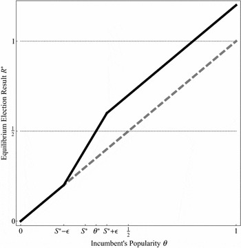
, and b = 70, which yield S* = 0.3, θ* = 0.35, ϕ* = 0.75, and w* = 3. That is, in equilibrium, agents engage in fraud only if the incumbent’s popularity in their precinct is greater than 30% and fraud secures the incumbent’s victory only if his national-level popularity is greater than 35%, or equivalently, when at least three-fourths of agents participate in fraud. Figure 2 employs these values to plot the equilibrium election result R* as a function of the incumbent’s genuine popularity θ.
The Effect of the Incumbent’s Genuine, National-level Popularity θ on the Equilibrium Election Result R* (solid black line)

We see in Figure 2 that the agents’ equilibrium behavior can be partitioned into four qualitatively distinct intervals over θ. At very low levels of the incumbent’s genuine popularity, 0 < θ < S* − ε, no agent observes a precinct-level popularity high enough to warrant engaging in fraud and all agents correctly anticipate the incumbent’s defeat. When S* − ε ⩽ θ < θ*, fraud occurs but fails: if enough agents engaged in fraud, they could ensure the incumbent’s victory for some values of θ on this interval, but because the incumbent’s popularity is too low, an insufficient number of agents ends up engaging in fraud. By contrast, when
 $\theta ^* \le \theta < \frac{1}{2}$
, enough agents engage in fraud to secure an undeserved victory for the incumbent. If we take the share of the election result that is due to fraud as a measure of such undeservedness, then the incumbent’s victory is most undeserved when θ = S* + ε and all agents engage in fraud. Finally, when
 $\frac{1}{2} < \theta < 1$
, fraud occurs but it is unnecessary: the incumbent is popular enough to win without fraud. In fact, when
 $\theta \ge \frac{1}{2} +\epsilon$
, all agents are aware that the incumbent will prevail without their complicity; they nonetheless engage in fraud because it boosts the election result in their precincts and thus leads to a higher reward. A perverse consequence of these incentives are national-level election results exceeding 100% at high values of θ.Footnote
24
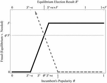
This conflict between the incumbent’s needs and the agents’ equilibrium behavior is illustrated in Figure 3. The bottom axis denotes the incumbent’s national-level popularity θ; the top axis denotes the equilibrium election result R*; the dashed gray line plots the level of fraud
 $\hat{F}$
that the incumbent needs for a victory; and the solid black line plots the level of fraud F* that occurs in equilibrium. When θ < θ*, the incumbent needs more fraud for a victory than the agents deliver,
 $F^*<\hat{F}$
. When θ ⩾ θ*, on the other hand, the agents engage in a level of fraud that is unnecessary from the incumbent’s point of view,
 $F^*>\hat{F}$
, collectively delivering up to 20% in excess of what the incumbent needs. Only at exactly θ* is the incumbent’s demand for fraud and its supply by the agents in balance: This is when the incumbent needs the national level of fraud to add up to 15% (ϕ*F = 0.15) and just the right fraction of agents—three-fourths (ϕ* = 0.75)—delivers it.
The Association between the Incumbent’s Genuine, National-level Popularity θ (bottom axis), the Equilibrium Election Result R* (top axis), the Equilibrium Level of Fraud F* (solid black line), and the Level of Fraud Needed for a Victory
 $\hat{F}$
(dashed gray line)

Realizations of the incumbent’s popularity across individual precincts thus play a central role in forming agents’ beliefs about the incumbent’s national-level popularity and, in turn, the degree of coordination needed for the incumbent’s victory. But the precise values of the thresholds S*, θ*, and ϕ* are also shaped by the parameters F, c, ε, b, and the equilibrium reward factor w*.
Consider the popularity threshold θ*, which is central not only strategically but also normatively: As θ* declines, the interval
 $\frac{1}{2}-\theta ^*$
along which the incumbent secures an undeserved victory becomes larger. An increase in the fraud capacity F and the reward factor w* lowers θ* and thus expands the range of θs along which the incumbent prevails in spite of being opposed by a majority of the electorate. That is, the greater the amount of fraud that each agent can produce within her precinct, the lower the demands on the agents’ coordination. Meanwhile, the greater the agents’ compensation for precinct-level results, the greater the risk that each agent is willing to take when engaging in fraud. The opposite holds for the cost parameter c. At borderline values of F, w*, and c (F → 0, w* → 0, or c → ∞), no fraud occurs in equilibrium when it is actually needed by the incumbent as
 $\theta ^*=\frac{1}{2}$
,
 $S^*=\frac{1}{2}+\epsilon$
, and ϕ* = 0. Intuitively, no agent is willing to risk prosecution when there is no way to inflate the incumbent’s vote share, when there is no personal benefit from doing so, or when the cost of failure is extreme.Footnote
25
Crucially, while a greater reward factor w* lowers the fraud and popularity thresholds S* and θ*, it does not eliminate the collective action problem among the agents.Footnote
26
Observe that as w* tends to infinity, lim
w → ∞ϕ* = 1, and in turn,
 $\lim _{w \rightarrow \infty } S^* = \frac{1}{2} - F - \epsilon$
and
 $\lim _{w \rightarrow \infty } \theta ^* = \frac{1}{2} - F$
, but
 $$\begin{equation*}
S^* > \frac{1}{2} - F - \epsilon \quad \text{and} \quad \theta ^* > \frac{1}{2} - F \quad \text{for any} \quad w^*>0.
\end{equation*}$$
That is, even when the agents’ compensation is arbitrarily large, there will be values of the incumbent’s popularity at which the agents could deliver the incumbent’s victory by conducting fraud but will fail to do so out of the fear that an insufficient fraction among them will engage in fraud.
Fraud as Insurance against Defeat: Pre-election Expectations and the Equilibrium Supply of Fraud
How do pre-election expectations about the incumbent’s popularity affect his choice of the agents’ reward w, and in turn, the equilibrium supply of fraud? In order to address this question, we must relax our assumption that θ is uniformly distributed on the entire interval (0, 1). This assumption in effect implied that the incumbent has no information about his likely national-level popularity on election day. In order to vary prior beliefs about θ, we now let θ be uniformly distributed on a smaller interval,
 $(\hat{\theta }-\sigma ,\hat{\theta }+\sigma )$
, with
 $\frac{F}{2} < \sigma < \frac{1}{2}$
.Footnote
27
We can therefore think of
 $\hat{\theta }$
and σ as the mean and degree of uncertainty in the incumbent’s and the agents’ pre-election expectations about θ.
In this extended setting, pre-election expectations about θ may vary from the pessimistic belief that unless he engages in fraud, the incumbent will lose the election for sure (when
 $\hat{\theta }+\sigma < \frac{1}{2} - F$
) to the optimistic belief that incumbent will win the election for sure even if he does not engage in any fraud (when
 $\hat{\theta }-\sigma > \frac{1}{2}$
). In turn, whenever
 $\hat{\theta } < \frac{1}{2} - F - \sigma$
or
 $\hat{\theta } > \frac{1}{2} + \sigma$
, the incumbent optimally sets w* = 0 since the agents’ actions cannot affect the election outcome. Meanwhile, when
 $\frac{1}{2} - F - \sigma \le \hat{\theta } \le \frac{1}{2} + \sigma$
, the equivalent of the incumbent’s expected payoff in (7) is
 $$\begin{equation}
\left(\frac{\hat{\theta }+\sigma - \theta ^*}{2 \sigma }\right) b - w \left(\hat{\theta } + \phi F \right) .
\end{equation}$$
Above, we used the fact that
 $E[\theta ]=\hat{\theta }$
and the equilibrium probability of the incumbent’s victory is now
 $\frac{\hat{\theta }+\sigma - \theta ^*}{2 \sigma }$
. Treating θ* and ϕ as functions of w and maximizing (8) with respect to w, we obtain
 $$\begin{equation*}
w^* = \sqrt{\frac{cF [\epsilon b + \sigma c F (2\epsilon +F)]}{\sigma [\hat{\theta }(2\epsilon + F) + F(2\epsilon + F -\frac{1}{2})]}} - c \, ,
\end{equation*}$$
which is decreasing in
$\hat{\theta }$
.
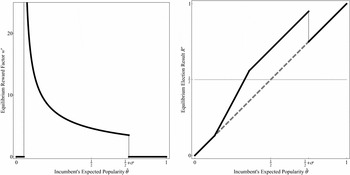
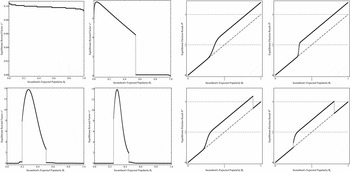
This result is illustrated in the left panel of Figure 4, which is based on
 $\sigma =\frac{1}{4}$
(keeping the remaining parameter values the same as in the basic model). Intuitively, as his expected popularity improves, the incumbent reduces the reward factor in order to avoid wasting resources on unnecessary fraud. Given the uncertainty in prior information about his eventual popular support θ, however, the incumbent is willing to pay his agents a positive reward factor even when he expects to prevail—hedging against the odds that he is being too optimistic. We may therefore view the incumbent’s choice of w as insurance against electoral defeat.
The Effect of Pre-election Expectations About the Incumbent’s Popularity
$\hat{\theta }$
on the Equilibrium Reward Factor w* (left) and the Expected Equilibrium Election Result R* (right)

The right panel in Figure 4 plots the effect of the incumbent’s expected popularity on the expected equilibrium outcome of the election (this is the analog of Figure 2 from our earlier discussion). We see that a key conclusion from our earlier analysis remains unchanged: in general, fraud is still either under- or oversupplied due to the interplay of the collective action and principal-agent problems in the execution of fraud. The key difference between our basic model and the present extension is that fraud no longer occurs when pre-election expectations about the incumbent’s popularity indicate that he can win the election without engaging in fraud. Clean elections can therefore arise out of two very different scenarios: in the first, the incumbent gives up on fraud because he desperately lacks popularity; in the second, the incumbent no longer bothers with fraud because he enjoys overwhelming popularity.
Differences in Competitiveness across Precincts: Persistent versus Variable Electoral Support
The previous extension introduced differences in pre-election expectations across elections but not across precincts. While the realizations of θ in our basic model do eventually differ across precincts, all precincts are ex-ante identical. In order to examine the consequences of differences in pre-election expectations across precincts, we now separate the incumbent’s support into two components, persistent and variable support. Variation across precincts in persistent support Pi captures the commonly known, ex ante differences between incumbent and opposition strongholds that exist in any real-world election. By contrast, we now refer to the privately observed and ex ante identical realizations Si as the incumbent’s variable support. The precinct-level result thus amounts to
 $$\begin{equation*}
R_i = \alpha P_i + (1-\alpha ) S_i + {\bf 1}_{\lbrace a_i=f\rbrace } F,
\end{equation*}$$
where α denotes the weight of persistent relative to variable support. This modification implies that the incumbent wins the election as long as
 $$\begin{equation*}
\alpha \pi + (1-\alpha ) \theta + \phi F \ge \frac{1}{2},
\end{equation*}$$
with π denoting the national-level average of the persistent component of the incumbent’s genuine support.
This distinction between persistent and variable components in the incumbent’s support suggests a change in the basis for agents’ rewards: rather then paying an agent by the overall result in her precinct, the incumbent now bases her reward on the difference between the overall precinct-level result Ri and the incumbent’s persistent precinct-level support Pi , since the latter is guaranteed and commonly known. Formally, each agent is promised the payoff w(Ri − Pi ). This implies that an agent who delivers 70% where the incumbent was expected to receive only 50% of the vote is rewarded more than one who delivers 90% where no less was expected in the first place. We derive the incumbent’s optimal choice of the reward factor as well as the equilibrium fraud, popularity, and majority thresholds in the Online Appendix.
This extension yields two intuitive insights. First, the equilibrium reward factor w* is decreasing in π, the national-level average of the persistent component. This result parallels that from the previous section as an increase in π amounts to a more optimistic expectation about the incumbent’s genuine popularity. Second, while the equilibrium supply of fraud is increasing in θ just as in the basic model, precincts with the largest realizations of variable support Si may not coincide with those where the result Ri is largest. Rather, fraud will be most abundant in precincts where the election outcome Ri exceeds pre-election expectations based on the persistent component Pi alone.
An Alternative Information Structure: The Normal Model
The key advantage of the uniform information structure that we have employed so far is the availability of closed form solutions for the fraud, popularity, and majority thresholds, and in turn, the ease with which their political implications can be studied. In order to establish the robustness of our results, we examine our model under an alternative information structure—the Normal model. Specifically, we denote by θ′ the probit-transformed version of the incumbent’s popularity θ and assume that it follows the Normal distribution with mean θ′
0 and variance σ2
0,
 $\theta ^{\prime } \sim \mathcal {N}(\theta _0^{^{\prime }},\sigma _0^2)$
. Analogously, we let S
′
i
denote the probit-transformed version of the agents’ signals Si
and assume that it follows the Normal density with the mean θ′ and variance σ2,
 $S^{^{\prime }}_{i} \sim \mathcal {N}(\theta ^{\prime },\sigma ^2)$
.Footnote
28
We transform θ′ and S
′
i
, whose support is on ( − ∞, ∞) onto (0, 1), the natural interval for θ and Si
, via the probit link, θ′ = Φ−1(θ) and S
′
i
= Φ−1(Si
).
An appealing feature of the Normal information structure is that it allows for prior beliefs about θ of an arbitrary mean and precision while maintaining a positive amount of uncertainty about θ and Si
along the entire support (0, 1). Unlike in the case of the uniform parametrization however, the threshold agent’s indifference condition for the Normal model does not have a closed form solution. Equilibrium fraud, popularity, and majority thresholds must therefore be obtained numerically.Footnote
29
Figure 5 illustrates the Normal model by plotting the effect of the pre-election expectation θ0 about the incumbent’s popularity on his equilibrium choice of the reward factor w* and the expected equilibrium election result R* at
 $\sigma _0^2=100,1,\frac{1}{25}$
, and
 $\frac{1}{100}$
(clockwise starting at top left).
The Effect of Pre-election Expectations About the Incumbent’s Popularity θ0 on the Equilibrium Reward Factor w* (left) and the Expected Equilibrium Election Result R* (right) for
 $\sigma _0^2=100,1,\frac{1}{25},\frac{1}{100}$
(clockwise starting at top left)

We see that key conclusions from our earlier analysis remain unchanged. As the right panel shows, fraud is either over- or undersupplied in equilibrium due to the interplay of the collective action and principal-agent problems. The key difference between the Uniform and the Normal models is that positive levels of fraud may occur at all values of θ in the latter. This is because even when θ is close to 0 (or 1), there is a small measure of agents who observe precinct-level signals implying that the incumbent is overwhelmingly popular (or unpopular) when the opposite is the case.
Figure 5 also indicates that the incumbent indeed views his choice w as insurance against electoral defeat. Given only vague prior information about his eventual popular support θ, the incumbent is willing to reward the agents for conducting fraud even when he expects to prevail, hedging against the odds that he is being too optimistic. While equilibrium comparative statics for the effect of σ2 0 on w* are mathematically too complex to be tractable, simulations suggest that as the precision of prior information about θ improves, the incumbent reduces the agent’s rewards at high and low levels of his expected popularity. This is consistent with our earlier discussion of w as insurance against defeat: when the incumbent expects an overwhelming victory, compensating the agents would only result in unnecessary fraud and thus be a waste of resources; when he expects an overwhelming defeat, any consequential reward factor would have to be so high as to render fraud too expensive.
EMPIRICAL ANALYSIS
Our theoretical analysis leads to a number of empirical predictions. First, incentive conflicts between the incumbent and his agents result in either the undersupply or oversupply of fraud. Second, a key feature of the herd dynamic that occurs among the incumbent’s agents is that small shifts in their perception of the incumbent’s viability may trigger large aggregate shifts in the amount of fraud conducted; this herd dynamic is strongest when the incumbent’s genuine popularity is close to the threshold θ*. Jointly, these predictions anticipate a pattern of elections that are won or lost by large margins correlated with the incumbent’s popularity. In these elections, the incumbent’s defeat may be instigated by only a minor decline in his genuine popularity, and while it may be widespread, electoral fraud will be politically decisive in only a fraction of the elections in which it occurs. Finally, our analysis predicts that the extent of fraud—and thus its fingerprints—should be increasing in both the incumbent’s genuine support as well as his vote share across precincts. Hence we should observe a positive association between the incumbent’s popularity and the extent of fraud across both multiple elections and individual precincts in a single election.
As a first step toward the empirical assessment of our arguments, we focus on the last of these predictions: That the extent of fraud across individual precincts should be increasing in the incumbent’s share of the vote. While fraud is difficult to identify in most elections, we take advantage of a particular form of fraud that arguably took place during the 2011 legislative and 2012 presidential elections in Russia: the rounding of the incumbent Vladimir Putin’s/United Russia Party’s precinct-level vote share to some higher multiple of 5 by the regime’s local operatives (Gehlbach Reference Gehlbach2012; Klimek et al. Reference Klimek, Yegorov, Hanel and Thurner2012; Kobak, Shpilkin, and Pshenichnikov Reference Kobak, Shpilkin and Pshenichnikov2012; Mebane Reference Mebane2013). Although this form of fraud was most likely only one among several forms of electoral manipulation during these elections, its execution at the level of individual precincts provides an opportunity to assess whether the extent of fraud was indeed increasing in the incumbent’s precinct-level vote share—as our theoretical model anticipates.
Several features of the 2011 legislative and 2012 presidential elections in Russia correspond to the key elements of our model. Extant empirical research as well as journalistic accounts indicate that fraud did indeed occur in these elections (Enikolopov et al. Reference Enikolopov, Korovkin, Petrova, Sonin and Zakharov2013);Footnote 30 that fraud was executed locally by operatives within the state bureaucracy, the public sector, and the United Russia party (Frye, Reuter, and Szakonyi Reference Frye, Reuter and Szakonyi2014); that these operatives where motivated by the promise of a political or bureaucratic advancement or monetary rewards—and often also by the complementary threat of demotion or dismissal (Reuter and Robertson Reference Reuter and Robertson2012);Footnote 31 that the regime had only rough information about its genuine support due to a proregime bias in public opinion surveys (Kalinin Reference Kalinin2013); and that the regime anticipated that unnecessary fraud might occur and wanted to avoid it unless it was needed for a first-round victory.Footnote 32 Due to space constraints, we focus below on the 2012 presidential election; our analysis of the 2011 parliamentary election—which provides even stronger support for our arguments—can be found in the Online Appendix.
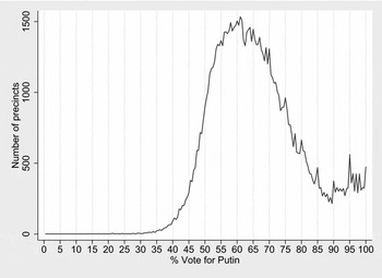
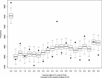
As a preliminary step, we establish that multiples of 5 are indeed over-represented in Vladimir Putin’s precinct-level vote shares. Figure 6 plots the distribution of Putin’s vote share in the 2012 presidential election across more than 90,000 precincts. In spite of the large number precincts, we see a suspicious lack of smoothness due to spikes that mostly coincide with multiples of 5, especially in the range 60–100%. In order to examine the distribution of digits in precinct-level vote shares more formally, we round each candidate’s vote share to the nearest multiple of 0.5, extract the unit and the first decimal place digits (e.g., both 76.481 and 46.532 become 6.5), and pool them into the 20 resulting digit pairs.Footnote 33 The frequencies of these pooled digit pairs in Vladimir Putin’s precinct-level results are displayed as triangles in Figure 7.
The Distribution of Vladimir Putin’s Precinct-level Vote Share in the 2012 Presidential Election

The Distribution of the Pooled Unit and the First Decimal Place Digits in Putin’s Precinct-level Vote Share (triangles) compared to the Distribution of Perturbed Values (the Whiskers in Box Plots Mark the 1st and the 99th percentiles)

Consistent with our discussion above, Figure 7 shows that precinct-level vote shares that end in either 0.0 or 5.0 are over-represented for Putin, and crucially, only for Putin. This is confirmed by a series of likelihood ratio independence tests (assuming that neighboring digits should be distributed approximately uniformly) as well as an alternative, perturbation approach. In the latter case, we follow Rozenas (Reference Rozenas2014) and slightly perturb the turnout and each candidate’s vote count across precincts and use these simulated values as our benchmark distribution.Footnote 34 The intuition behind this approach is to ask: If this election were rerun thousands of times with a realistic variation in turnout and voting decisions, how likely is it that this many multiples of 5 would occur naturally? The answer is extremely unlikely—definitely beyond conventional levels of statistical significance. The whiskers of the box plots in Figure 7 mark the 1st and 99th percentiles of the perturbation simulations, and we see that 0.0 and especially 5.0 are the most significantly over-represented digit pairs.Footnote 35
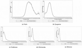
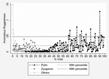
We now turn to our main empirical test and examine whether the over-representation of the multiples of 5 for Putin is indeed increasing in his precinct-level vote share as predicted by our model. In order to do so, we first need to develop a measure of the ruggedness in the distribution of Putin’s precinct-level results. We use two different approaches: the first employs kernel density estimation techniques; the second is based on the perturbation approach that we just discussed. The first approach measures the ruggedness in the distribution of a candidate’s precinct-level results by taking the difference between that distribution and its optimal kernel density estimate.Footnote 36 The empirical distribution corresponds to a histogram with 0.5 bin width; the kernel density estimate employs the (optimal) Epanechnikov kernel and the optimal bandwidth estimate.Footnote 37 Figure 8 plots the kernel density estimate of each candidate’s precinct-level results with a black dashed line along with their actual empirical distribution (gray solid line). We see a nearly perfect overlap between the distribution of precinct-level vote shares and the corresponding kernel density estimates for the three minor candidates (Prokhorov, Zhirinovsky, and Mironov), some ruggedness unrelated to multiples of 5 for Zyuganov, and significant ruggedness correlated with multiples of 5 for Putin.
The Distribution (gray solid line) and Kernel Density Estimate (black dashed line) of Each Candidate’s Precinct-level Results

Figure 8 further highlights that the ruggedness in the distribution of Putin’s precinct-level results is not only substantial but also increasing in his precinct-level vote share, as our theoretical framework anticipated. In order to quantify how anomalous this ruggedness is and to evaluate the strength of its association with Putin’s precinct-level vote share, we judge Putin by the standard of his four competitors. Specifically, we calculate the difference between the empirical distribution of Putin’s competitors’ precinct-level results and their kernel density estimate, pool these residuals, and use their 95th and 99th percentiles as our first benchmark for judging how anomalous the ruggedness of Putin’s precinct-level results is.Footnote 38 Figure 9 plots these residuals separately for Putin (diamonds), Zyuganov (squares), and the remaining three minor candidates (Prokhorov, Zhirinovsky, and Mironov). We see that with the exception of a few poorly fitting corner values for the minor candidates, all residuals above the 95th and 99th percentile benchmarks belong to either Putin or Zyuganov. Crucially, only Putin’s residuals coincide with the multiples of 5 and are significantly increasing in his vote share.Footnote 39
The Difference between the Empirical Distribution of Each Candidate’s Precinct-level Results and its Kernel Density Estimate

We arrive at identical conclusions when we employ an alternative, perturbation benchmark for evaluating the ruggedness of Putin’s precinct-level results. Just as we did earlier in the case of digit frequencies, we perturb the turnout and each candidate’s vote count across precincts, compute the 95% and 99% confidence intervals using these simulated values, and treat the observations that lie outside these confidence intervals as anomalously rugged. Just as before, Putin’s and Zyuganov’s residuals are significantly larger than those of the remaining candidates and only Putin’s residuals are increasing in his precinct-level vote share.Footnote 40 Hence judging by two different standards—that of Putin’s competitors and perturbation-based confidence intervals—the distribution of Putin’s results is indeed suspiciously rugged at multiples of 5 and this ruggedness is increasing in his precinct-level vote share—as anticipated by our theoretical arguments.
To summarize, our analysis of the 2011–2012 Russian legislative and presidential elections (see the Online Appendix for the former) supports a key prediction from our theoretical model: The extent of fraud in these elections is indeed increasing in the incumbent Vladimir Putin’s and United Russia’s precinct-level vote share and, crucially, in only their vote share. We took advantage of a particular type of fraud that occurred during these elections—the rounding of the regime candidate’s and party’s vote share to some higher multiple of 5. Consistent with the findings from earlier analyses of these elections, we found that precinct-level vote shares corresponding to multiples of 5 are indeed over-represented in Putin’s and United Russia’s results but not those of other candidates or parties.Footnote 41
Nonetheless, there are some questions about these elections that our data and methods do not allow us to address. Chief among them is why fraud took the particular form of the rounding of the incumbent’s precinct-level vote share to some higher multiple of 5. Plausible explanations include regional targets that themselves were multiples of 5, attempts by local operatives to signal complicity without leaving direct evidence (cf. Kalinin and Mebane Reference Kalinin and Mebane2011), or the human tendency to fabricate numbers that are multiples of 5 (cf. Kobak, Shpilkin, and Pshenichnikov Reference Kobak, Shpilkin and Pshenichnikov2014). Unfortunately, we cannot discriminate among these conjectures with the available data. Our results—just like many qualitative accounts of fraud during these elections—also indicate that a different method of manipulation was employed in some ethnic republics and “special” precincts (e.g., hospitals and military units). Results from these places show turnout and vote-share for the regime that are unrealistically close to 100%, suggesting that they were delivered wholesale with fraud that was executed at the top rather than the bottom of the administrative hierarchy. Finally, we are unable to eliminate the alternative hypothesis that anomalies indicative of fraud may be increasing in Putin’s and United Russia’s precinct-level vote share because observers, local electoral commission members, or even ordinary citizens are less likely to deter fraud in precincts where the regime is highly popular.Footnote 42
CONCLUSION
Why do incumbents who could arguably win a clean election engage in fraud? Our analysis of the principal-agent and collective action problems in the political organization of electoral fraud suggests an answer. Because most fraud is ultimately executed by a large number of local operatives with an incentive to conceal their actions, incumbents’ control over whether and how much fraud will be conducted is limited. Each agent understands that the difference between her promotion and prosecution rests on whether her involvement in fraud will result in the incumbent’s eventual victory or defeat. In turn, the agents’ perception of the incumbent’s popularity and the ensuing burden on their collective complicity plays a crucial coordinating role. The aggregate result is too much fraud for incumbents who need it the least and too little fraud for those who need it the most. The seeming invincibility of some incumbents and the surprising fragility of others are thus two sides of the same political logic.
Our analysis of the 2011–2012 Russian legislative and presidential elections finds support for one prediction based on these intuitions: that the extent of fraud should be increasing in the incumbent Vladimir Putin’s and United Russia’s precinct-level vote share. Yet this prediction is only one among several implied by our theory. The Russian case, along with pre-1980s Mexico (illustrated by the quotation in our epigraph), and Daniel Ortega’s Nicaragua (especially the 2008 local and 2011 presidential elections), illustrates the scenario in which an incumbent employs fraud as insurance against defeat, with its oversupply becoming the undesirable byproduct when that insurance proves unnecessary. A more comprehensive assessment of our arguments should also evaluate our predictions about the undersupply of fraud that obtains when the machinery of fraud is reluctant to follow an incumbent with a declining popularity—as in the case of the presidential elections in Mexico (1988 and 2000), Senegal (2012), and Sri Lanka (2015).
Our arguments apply most directly to political systems that have been alternately referred to as hybrid, electoral authoritarian, or competitive authoritarian regimes (Bunce and Wolchik Reference Bunce and Wolchik2011; Levitsky and Way Reference Levitsky and Way2010; Schedler Reference Schedler2013). A distinguishing feature of these regimes is the presence of elections that are competitive enough to allow for an active opposition yet at the same time systematically favor the incumbent.Footnote 43 Our analysis explains why these regimes may be significantly more fragile than existing research admits. Even if the infrastructure of fraud favors the incumbent, his genuine popularity still plays a crucial role in shaping the agents’ perception of the risk of engaging in fraud. Electoral authoritarianism should therefore be characterized by a punctuated dynamic, with an oversupply of fraud that lasts as long as the incumbent enjoys genuine popularity and is interrupted by an undersupply of fraud as soon as that popularity dwindles. Even manipulated elections thus hold the potential for a democratic opening.
This logic further suggests that strong parties and obedient bureaucracies—whose “organizational power” is often evoked as a source of stability in these regimes—are merely symptoms rather then the underlying causes of regime persistence. After all, organizational power ultimately depends on the willingness of hundreds of bureaucrats and apparatchiks to obey the incumbent’s orders and is therefore endogenous to these agents’ perception of his political prospects. Bureaucrats and apparatchiks understand all too well that the difference between their promotion and their prosecution for illegally aiding an incumbent is in whether the incumbent ultimately survives in office. To put it metaphorically: when the incumbent looks like a success, organizational power has a thousand fathers.
Our analysis of the political organization of electoral fraud suggests a number of directions for future research. Our model intentionally focuses on forms of manipulation that may be classified as locally executed, election-day fraud. This category captures some of the most frequent forms of fraud: ballot box stuffing, voter intimidation, count falsification, vote buying, multiple voting, etc. Nonetheless, these forms of fraud are frequently preceded and sometimes followed by their centrally executed counterparts. Our results point to several trade-offs inherent in a regime’s decision about the timing and level of manipulation. As we have shown, incumbents who rely on locally executed election-day fraud end up with only limited control over how much of it will be conducted. By contrast, top-level election-day fraud provides such control—since it amounts to the rewriting of the election result by the incumbent—but it is brazen and therefore best used as a weapon of last resort. Manipulation before the election, meanwhile, allows for more subtle ways of stacking the deck against the opposition, but because of its timing, it remains vulnerable to public exposure and condemnation by the opposition. Future research should account for these trade-offs explicitly, by incorporating the choice of the timing and level of manipulation within a single model.
Our framework also highlights a novel, distinctively political feature of the principal-agent problem in the execution of electoral fraud. Just like in many other political and economic agency problems, the incumbent—the principal—observes the agents’ actions only imperfectly. Specifically, the incumbent cannot condition the agents’ reward on the actual amount of fraud since the latter is intentionally concealed. Yet, unlike in most settings, the principal’s problem is further complicated by the politically conditional nature of the agents’ rewards: the agents know that they will obtain the promised rewards only if the incumbent eventually wins the election.
To facilitate our analysis of this principal-agent problem, we worked with a simple reward structure, according to which the agents’ rewards linearly increase in the precinct-level election outcome—but only if the incumbent wins.Footnote 44 Yet real-world fraud reward structures are never written or even explicitly stated, often include a mix of positive and negative incentives, and are typically embedded within the institutional infrastructure of regime parties and government bureaucracies. Future research should explain these qualitative features of the political organization of electoral fraud as an optimal choice within a more general model of political agency.
Our analysis of principal-agent and collective-action problems in the political organization of electoral fraud naturally extends to other settings, most directly to patronage politics, election campaigns, and repression. Just as in the present setting, the rewards and punishment of patronage brokers, campaign operatives, and repressive agents are contingent upon the success or survival of their principals.Footnote 45 In patronage politics, for example, a broker’s effort on behalf of a candidate is critically shaped by her expectation of the candidate’s ultimate victory and hence the likelihood that her effort will not be wasted.Footnote 46 Meanwhile in repression, the willingness of a repressive agent to engage in legally questionable suppression of opposition depends on his expectation of the regime’s survival and hence his immunity from prosecution. Just as in the case of fraud, candidates and leaders who want to motivate their operatives to engage in electioneering or repression have only limited control over whether and how much of it will eventually be conducted. This is because patronage brokers, campaign operatives, and repressive agents have one key thing in common: they all want to work for a winner.
SUPPLEMENTARY MATERIAL
To view supplementary material for this article, please visit http://dx.doi.org/10.1017/S0003055415000635









Comments
No Comments have been published for this article.