



1. Introduction
Flow-induced instabilities of bluff bodies arise from the interaction between the aerodynamic forces and the dynamics of the structure and constitute a classical class of fluid–structure interaction problems. Depending on the relative time scales of the flow and the solid response, such interactions may lead to a variety of self-excited or resonance-driven motions, including vortex-induced vibrations (VIV) and galloping (Blevins Reference Blevins2001; Païdoussis et al. Reference Païdoussis, Price and De Langre2010). These phenomena have been studied extensively because of their rich underlying physics and their occurrence in systems ranging from laboratory-scale model problems to large-scale structures exposed to wind or currents: bridges (Parkinson Reference Parkinson1971; Matsumoto et al. Reference Matsumoto, Shiraishi and Shirato1992), cable cars (Brownjohn Reference Brownjohn1998; Hofman Reference Hofman2009), slung loads transportation (Oktay & Sultan Reference Oktay and Sultan2013; Jin et al. Reference Jin, Liu, Zheng and Chen2020) or offshore platforms for instance.
A key parameter governing the nature of flow-induced responses is the ratio between the characteristic time scale of the body motion and that of the flow, commonly expressed through the reduced velocity
 $U^*=U_0/(Df)$
, where
 $U_0$
is the free-stream velocity,
 $D$
the characteristic length of the body and
 $f$
the characteristic frequency of its motion. At moderate reduced velocities, typically
 $U^*\leq 10$
for a rectangular cylinder and
 $U^*\approx 5$
for a circular cylinder, the interaction between the body motion and coherent vortex shedding in the wake may lead to VIV characterised by lock-in and resonance phenomena (Parkinson & Brooks Reference Parkinson and Brooks1961; Bearman et al. Reference Bearman, Gartshore, Maull and Parkinson1987; Zhao et al. Reference Zhao, Leontini, Lo Jacono and Sheridan2014). As the reduced velocity increases, the influence of vortex shedding diminishes and the aerodynamic forces acting on the body may be described, to leading order, within a quasi-steady framework. In this regime, the system may undergo galloping, a self-excited instability driven by negative aerodynamic damping and sustained by a net transfer of energy from the flow to the structure (Blevins Reference Blevins2001; Païdoussis et al. Reference Païdoussis, Price and De Langre2010).
The vortex shedding dynamics is weaker and less coherent in the wake of a three-dimensional bluff body than in the wake of a two-dimensional cylinder (Tamura & Miyagi Reference Tamura and Miyagi1999; Zhao et al. Reference Zhao, Sheridan, Hourigan and Thompson2019; Kozmar Reference Kozmar2021): a three-dimensional geometry is thus much less favourable to VIV. Cross-flow galloping also exists on three-dimensional bluff bodies like a cube and is driven by similar mechanisms as for a two-dimensional cylinder (Zhao et al. Reference Zhao, Sheridan, Hourigan and Thompson2019; Cheng et al. Reference Cheng, Zhang, Wang, Lien and Dowell2024; Myskiw et al. Reference Myskiw, Haffner, Paillé, Borée and Sicot2024).
Galloping has been investigated in detail for canonical configurations involving elastically mounted bluff bodies with a single dominant degree of freedom (DoF), most commonly in the cross-flow direction. For two-dimensional rectangular cylinders (including square cylinders), the onset of galloping has been successfully predicted using quasi-steady models, provided that the reduced velocity is sufficiently large to avoid coupling with VIV (Parkinson & Smith Reference Parkinson and Smith1964; Nakamura & Tomonari Reference Nakamura and Tomonari1977; Parkinson & Wawzonek Reference Parkinson and Wawzonek1981). The classical Den Hartog criterion relates the stability of the equilibrium state to the slope of the transverse force coefficient with respect to the angle of attack and remains a cornerstone of galloping theory (Den Hartog Reference Den Hartog1932, Reference Den Hartog1985). This criterion can be obtained from the linearisation of the equations of dynamics or from the linearisation of the periodic energy balance between the body and the flow. Experimental and numerical studies have shown that galloping is strongly dependent on the body geometry and on the turbulence of the flow, which influences the aerodynamic coefficients of the body and their gradients, in particular via flow separation and reattachment characteristics: a fully separated flow on the sides of the body promotes instability, whereas partial flow reattachment tends to stabilise the system (Parkinson Reference Parkinson1971; Nakamura et al. Reference Nakamura, Hirata and Urabe1991). Therefore, the increase of the streamwise aspect ratio of the body is stabilising as it is conducive to flow reattachment on its sides (Parkinson & Brooks Reference Parkinson and Brooks1961; Hémon & Santi Reference Hémon and Santi2002). The rounding of the front edges of a rectangular cylinder also has a stabilising effect regarding galloping as it promotes flow reattachment: the flow bypassing a front edge is less deflected by a rounded edge than by a sharp one (Tamura & Miyagi Reference Tamura and Miyagi1999; Carassale et al. Reference Carassale, Freda and Marre-Brunenghi2013). In addition, an increase of the upstream flow turbulence intensity results in an increase of the diffusion of the shear layer downstream separation, promoting flow reattachment on the sides of the body and thus stabilising the body regarding galloping (Nakamura & Ozono Reference Nakamura and Ozono1987; Carassale et al. Reference Carassale, Freda and Marre-Brunenghi2013).
Three-dimensional bluff body pendulums like disks, plates or cubes with 1 DoF in the cross-flow or streamwise direction can be subjected to different types of flow-induced instabilities, including bistability, VIV or galloping (Obligado et al. Reference Obligado, Puy and Bourgoin2013; Fani & Gallaire Reference Fani and Gallaire2015; Orchini et al. Reference Orchini, Kellay and Mazzino2015; Gayout et al. Reference Gayout, Bourgoin and Plihon2021; Bao et al. Reference Bao, Plihon and Bourgoin2025). The onset of cross-flow galloping for a cube pendulum is driven by the same mechanisms as for two-dimensional cylinders, and thus, can be predicted using the Den Hartog criterion: the oscillations start from rest, amplify and end up saturated at a constant amplitude. Unsteady dynamics rise during the development of the oscillations and drive the saturation of the swinging motion, characterised by periodic flow separation–reattachment on the sides of the cube (Myskiw et al. Reference Myskiw, Haffner, Paillé, Borée and Sicot2024). Indeed, by comparison with an elastically mounted body, the equivalent stiffness of the pendular system due to the gravity restoring force decreases with the amplitude of oscillation; therefore, a pendulum undergoing a galloping instability can reach larger amplitudes than an elastically mounted body.
Multiple degrees of freedom allow coupled motions and extend the field of flow-induced vibrations. Typical configurations include elastically mounted bluff bodies free to oscillate in the cross-flow and streamwise directions (Jauvtis & Williamson Reference Jauvtis and Williamson2004; Rajamuni et al. Reference Rajamuni, Thompson and Hourigan2019; Carlson et al. Reference Carlson, Currier and Modarres-Sadeghi2021). The case of a submerged tethered buoyant sphere, or equivalently, a heavy sphere pendulum in air flow, also received a particular attention (Govardhan & Williamson Reference Govardhan and Williamson1997; Mathai et al. Reference Mathai, Loeffen, Chan and Wildeman2019; Rajamuni et al. Reference Rajamuni, Thompson and Hourigan2020; Kovalev et al. Reference Kovalev, Eshbal and Van Hout2022; Gold et al. Reference Gold, Reiterer, Worf, Kaiblinger, Khosronejad, Habersack and Sindelar2024). These studies mainly focus on VIV and highlight a coupling between the streamwise and cross-flow oscillations. Because of the periodic symmetry of the wake, the vortex dynamics induces a forcing frequency on the body in the streamwise direction twice larger than that induced in the cross-flow direction, which allows eight-shaped or butterfly shaped trajectories. In case of galloping, no such symmetry exists in the wake so a system characterised by the same natural frequencies for both degrees of freedom (like a pendulum driven by gravity) can only have unidirectional or quasi-elliptical trajectories. The case of a slung three-dimensional prisms with multiple degrees of freedom in a flow has also been investigated by Jin & Chamorro (Reference Jin and Chamorro2017) at significant reduced velocities
 $U^*\in [8\,;\,36]$
conducive to the rise of the galloping instability.
The galloping instability of a 2-DoF bluff body pendulum much denser than air is studied from experimental and theoretical approaches in the present work. As the focus is on the galloping instability, large reduced velocities out of the VIV range are investigated (
 $U^*\gt 20$
). The application in ropeway transport initially motivated this work, so a cube pendulum is experimentally studied in a wind tunnel as this shape can be seen as a simplified model of a cable car. The equations of the pendulum dynamics highlight two important parameters: the mass number
 ${\mathcal{M}}=\rho _{\textit{air}}/\rho _{{body}}$
defined from the density of the body
 $\rho _{{body}}$
and the density of the air
 $\rho _{\textit{air}}$
, and the Froude number
 $F_r=U_0/\sqrt {gL_0}$
defined from the flow velocity
 $U_0$
, the equivalent pendulum length
 $L_0$
and the gravitational acceleration constant
 $g$
. As the considered pendulum is ‘heavy’, meaning that it is much denser than air, the mass number is very low (
 ${\mathcal{M}}\sim 10^{-3}$
). The Froude number is proportional to
 $U^*$
and have consistently moderate to large values (
 $F_r\in [2.4\,;\,14.2]$
). The Reynolds number
 $\textit{Re}\sim 10^5$
falls into the turbulent flow regime and is not a parameter of the study, the considered model having sharp edges.
To the author’s knowledge, no other dedicated experimental or numerical framework for a 2-DoF three-dimensional bluff body pendulum at this range of reduced velocities can be found in the literature. A method is proposed from a quasi-steady approach to identify the main aerodynamic parameters influencing the stability of such a system and to predict the onset of the galloping instability. This method is based on the analysis of the energy transfers between the pendulum and the flow and considers the pseudo-periodic behaviour specific to the pendulum to identify the stability factors.
The paper is organised as follows. Section 2 introduces the general characteristics of the type of pendulum considered, the associated equations of the pendulum dynamics and the experimental set-ups used to study the stability of a cube pendulum in a wind tunnel. The experimental stability analysis on the cube pendulum is detailed in § 3. The physical mechanisms driving the onset of a galloping are then analysed in § 4 from two distinct approaches. First, an energy-based quasi-steady linear model is developed in § 4.1 and highlights the most influent parameters regarding the pendulum stability (§§ 4.2 and 4.3). An example of the use of the model as a prediction tool is introduced in § 4.4. Then, the pressure measurement on the cube pendulum is used to investigate quasi-steady or unsteady flow mechanisms observed at the onset of galloping in §§ 4.5 and 4.6.
2. Pendulum system and experimental set-ups
2.1. Introduction of the pendulum system
The pendulum considered is much denser than the air and is made of two rigid solids: a bluff body of characteristic length
 $D$
attached to a rod of length
 $H$
. Here
 $D$
and
 $H$
are of the same order of magnitude. The bluff body used in this study is a cube of side length
 $D$
as depicted in figure 1(a). A punctual joint at the extremity of the rod allows the pendulum to rotate with 2 DoF, in the cross-flow and streamwise directions, but the rotation of the body around the rod is blocked. The length between the joint (O) and the geometric centre of the body (C) is denoted
 $L$
and is referred to as the real pendulum length. The distance between the joint (O) and the gravity centre of the pendulum (G) is denoted
 $L_g$
.
The characteristic pulsation of the pendulum is written
 $\omega _0$
and can be expressed from the characteristic oscillation period of the pendulum
 $T_0$
(period for small-amplitude swings) or the equivalent pendulum length
 $L_0$
, such as
 $\omega _0=2\pi /T_0=\sqrt {g/L_0}$
. The equivalent pendulum length
 $L_0$
corresponds to the length of a simple point-like pendulum with the same characteristic period. Here
 $g$
refers to the gravitational acceleration constant.
The bluff body is much bigger and heavier than the rod, such that the aerodynamic loads applied on the rod can be neglected compared with those applied on the body. The mass of the pendulum, referred to as
 $m$
, is thus mainly composed of the body mass. A cube has several orthogonal symmetry planes intersecting on the rod axis. Its mass distribution is assumed symmetrical with respect to these planes, such that the gravity centre of the pendulum (G) is located on the arm axis, as depicted in figure 1(a). These characteristics regarding the geometry and the mass distribution of the body are used to simplify the equation of dynamics. They are not specific to the cube: cylindrical (square or circular cylinders for instance) or ovoid shapes (sphere included) share the same characteristics. The modelling of the pendulum dynamics proposed in this work can be applied to any bluff body that meets these conditions.
(a) Definition of the cube pendulum. (b) Definition of the initial yaw angle
 $\beta _0$
between the cube and the free-stream velocity
 $\boldsymbol{U_{0,\theta }}=(\boldsymbol{U_0}\boldsymbol{\cdot }\boldsymbol{e_\theta })\,\boldsymbol{e_\theta }$
. (c) Definition of the spherical frame
 $({\boldsymbol{e_r}}, \boldsymbol{e_\theta }, \boldsymbol{e_\phi })$
from the fixed reference frame
 $({\boldsymbol{x}}, \boldsymbol{y}, \boldsymbol{z})$
. (d) Free-body diagram representing the resisting moment due to the friction at the joint
 $\boldsymbol{M_{\!f}}$
and the moments
 $\boldsymbol{M_a}$
and
 $\boldsymbol{M_{\!g}}$
produced by the aerodynamic and gravity forces
 $\boldsymbol{F_a}$
and
 $\boldsymbol{F_g}$
(
 $\boldsymbol{F_a}$
is the ‘fictive’ aerodynamic force applied at C).

Figure 1. Long description
Panel A: A 3D view of a cube pendulum system. The diagram shows a cube suspended by an arm from a joint. The cube has dimensions labeled as L, H, and D. The arm has a length labeled as Lg. The angle beta0 is shown between the arm and the vertical. The center of gravity of the cube is marked as G, and the point of contact with the fluid is marked as C. Panel B: A top view of the cube pendulum. The initial yaw angle beta0 is defined between the cube and the free-stream velocity U0,theta. The point C is marked, and the unit vectors er, etheta, and ephi are shown. Panel C: A spherical frame definition from the fixed reference frame. The origin is at point O, and the unit vectors er, etheta, and ephi are shown in 3D space. The angles phi and theta are defined, and the free-stream velocity U0 is shown. Panel D: A free-body diagram representing the forces and moments acting on the cube pendulum. The gravity force Fg acts downward, the fictive aerodynamic force Fa acts at point C, and the resisting moment due to friction at the joint is shown. The moments Mg, Ma, and Mf are represented by arrows indicating their directions.
The incoming wind is horizontal with a mean velocity
 $U_0$
. Two frames are introduced to describe the pendulum dynamics, using the centre of the pendulum joint, denoted
 $O$
, as the origin (figure 1
c):
-
(i) the fixed reference frame
 $({\boldsymbol{x}}, \boldsymbol{y}, \boldsymbol{z})$
where
$\boldsymbol{x}$
is the wind direction and
$\boldsymbol{z}$
the vertical axis;
-
(ii) the moving spherical frame
$({\boldsymbol{e_r}}, \boldsymbol{e_\theta }, \boldsymbol{e_\phi })$
defined from the two angles used to get the position of the pendulum: the longitudinal angle
$\theta$
(around
$\boldsymbol{e_\phi }$
) and the lateral angle
$\phi$
(around
$\boldsymbol{x}$
);
$\boldsymbol{e_r}$
is the rod axis directed from the body to the joint,
$\boldsymbol{e_\phi }$
is in the plane
$(\boldsymbol{y},\boldsymbol{z})$
and corresponds to
$\boldsymbol{y}$
if
$\phi =0$
,
$\boldsymbol{e_\theta }$
is in the plane
$({\boldsymbol{x}},{\boldsymbol{e_r}})$
and corresponds to
$\boldsymbol{x}$
if
$\theta =0$
;
$\theta \lt 0$
when the pendulum tilts backwards.


The change-of-basis matrix from the fixed reference frame to the spherical frame and the angular velocity vector
 $\boldsymbol{\varOmega }$
of the pendulum about O are given as (note that all the equations, matrices and vectors introduced are written in the spherical frame):
 \begin{equation} \begin{array}{cc}&\begin{array}{ccc} {\boldsymbol{x}} \qquad & \qquad \boldsymbol{y} & \qquad\qquad \boldsymbol{z} \end{array}\\ &\begin{array}{c} {\boldsymbol{e_r}} \\[3pt] \boldsymbol{e_\theta } \\[3pt] \boldsymbol{e_\phi } \\ \end{array}\!\!\! \begin{pmatrix} \sin (\theta ) & -\cos (\theta ) \sin (\phi ) & \cos (\theta ) \cos (\phi ) \\[3pt] \cos (\theta ) & \sin (\theta ) \sin (\phi ) & - \sin (\theta ) \cos (\phi ) \\[3pt] 0 & \cos (\phi ) & \sin (\phi ) \\ \end{pmatrix}\end{array} \!\!,\quad \boldsymbol{\varOmega } = \begin{array}{cc} \begin{pmatrix}{} 0 \\ \dot {\phi } \, \cos (\theta ) \\ \dot {\theta } \\ \end{pmatrix} \!\!\! \begin{array}{c} {\boldsymbol{e_r}} \\ \boldsymbol{e_\theta } \\ \boldsymbol{e_\phi } \\ \end{array} \!.\end{array} \end{equation}
The initial yaw angle
 $\beta _0$
refers to the yaw angle of the bluff body defined from the projection of the free-stream direction in the plane orthogonal to the arm axis
 $(\boldsymbol{e_\theta },\boldsymbol{e_\phi })$
, as illustrated in figure 1(b). This angle remains fixed during motion as the cube cannot rotate around the arm axis.
Two main external forces act on the pendulum: the gravity force and the aerodynamic force, applied respectively at the centre of mass
 $G$
and at the centre of pressure
 $A$
. Here
 $G$
is fixed and aligned with the arm axis
 $\boldsymbol{e_r}$
due to the symmetrical mass distribution of the body, whereas the position of
 $A$
slightly varies around the geometric centre of the body according to the orientation of the pendulum and its dynamics. Instead of modelling its displacement in the equations of dynamics,
 $A$
is considered fixed at the geometric centre of the body
 $C$
(
 $\boldsymbol{{AO}}=\boldsymbol{{CO}}=L{\boldsymbol{e_r}}$
), and the aerodynamic moment
 $\boldsymbol{M_a}$
applied at O is expressed from the ‘fictive’ aerodynamic force
 $\boldsymbol{F_a}$
such that
 $\boldsymbol{M_a}=\boldsymbol{F_a}\times \boldsymbol{{CO}}$
(figure 1
d). The aerodynamic force coefficients along
 $\boldsymbol{e_\theta }$
and
 $\boldsymbol{e_\phi }$
used in the equation of dynamics thus consider the additional moments due to the displacement of the centre of pressure, as detailed later in the paper (see (2.4) in § 2.3). These coefficients are respectively written as
 $C_\theta$
and
 $C_\phi$
. As the application points of both forces are assumed located on the arm axis
 $\boldsymbol{e_r}$
, no resulting moments are produced about this axis. In addition to the aerodynamic and gravity forces, the mechanical friction at the joint is modelled by a viscous damping that produces a resisting moment (figure 1
d), expressed using the damping coefficients
 $\lambda _1$
and
 $\lambda _2$
respectively associated to the rotation of the pendulum around
 $\boldsymbol{e_\theta }$
and
 $\boldsymbol{e_\phi }$
. Finally, the arm of the pendulum is fully rigid so its longitudinal and torsional stiffness are assumed infinite and, thus, do not develop any moment able to influence the pendulum dynamics.
The balance of the moments acting on the pendulum applied at
 $O$
is written about the two axes of motion
 $\boldsymbol{e_\theta }$
and
 $\boldsymbol{e_\phi }$
, as formulated in the non-dimensional equation
 \begin{equation} \begin{aligned} \frac {1}{\omega _0^2}\, \begin{pmatrix} \ddot {\phi } \,\cos (\theta ) - 2 \dot {\theta }\dot {\phi } \,\sin (\theta ) \\[3pt] \ddot {\theta } + \dot {\phi }^2\,\cos (\theta )\sin (\theta ) \end{pmatrix} &= \frac {1}{2} \, r_g \, l_0\, \mathcal{M} F_r^2 \begin{pmatrix} C_\phi \\[3pt] -C_\theta \end{pmatrix} - \begin{pmatrix} \sin (\phi ) \\[3pt] \sin (\theta )\cos (\phi ) \end{pmatrix} \\ &\quad - \frac {2}{\omega _0^2} \begin{pmatrix} \lambda _1 \,\dot {\phi } \, \cos (\theta ) \\[3pt] \lambda _2 \, \dot {\theta } \end{pmatrix} \!.\end{aligned} \end{equation}
The expressions and developments leading to this equation are detailed in Appendix A.
-
(i) The ratio between the pendulum length and the distance from the centre of mass to the joint is
$r_g=L/L_g$
. In the frame of the study,
$r_g\sim 1$
as the pendulum mass is mainly made of the bluff body mass. -
(ii) The ratio between the equivalent pendulum length and the characteristic length of the body is
$l_0=L_0/D$
. The similar ratio
$l=L/D$
between the real pendulum length and the characteristic length of the body is also used later in the study. -
(iii) The Froude number based on the equivalent pendulum length is
$F_r=U_0/\sqrt {g L_0}=U_0/(L_0\,\omega _0)=U^*/(2\pi \,l_0)$
. It is proportional to the reduced velocity
$U^*$
. -
(iv) The mass number (the expression of the total volume of the pendulum is approximated by
$SD=D^3$
, with
$S=D^2$
the reference surface) is
$\mathcal{M}=\rho _{\textit{air}}/\rho _{{body}}=\rho S D/m$
. Here
$\mathcal{M}\lt \lt 1$
as the pendulum is much denser than air.


The pendulum at equilibrium is immobile at a position where the moments produced by the aerodynamic and gravity forces are balanced, i.e.
 \begin{equation} \frac {1}{2} \, r_g \, l_0\, \mathcal{M} F_r^2 \begin{pmatrix} \overline {C_\phi } \\[3pt] -\overline {C_\theta } \end{pmatrix} - \begin{pmatrix} \sin (\overline {\phi }) \\[3pt] \sin (\overline {\theta })\cos (\overline {\phi }) \end{pmatrix} = \begin{pmatrix} 0 \\ 0 \end{pmatrix} \!. \end{equation}
The angles
 $\theta$
and
 $\phi$
of the pendulum at equilibrium are denoted as
 $\overline {\theta }$
and
 $\overline {\phi }$
. Similarly,
 $\overline {C_{\theta ,\phi }}$
refer to the aerodynamic coefficients at equilibrium. In this situation, the yaw angle of the pendulum equals the static yaw angle
 $\beta _0$
. The pitch angle at equilibrium, written
 $\alpha _0$
, corresponds to the longitudinal angular position of the pendulum:
 $\alpha _0=-\overline {\theta }$
. The definitions of the aerodynamic angles of the pendulum are detailed in Appendix A.
2.2. Cube pendulum set-up
A cube pendulum is implemented in the test section of
 $2.4\times 2.6\,\text{m}^2$
of the subsonic closed-loop wind tunnel S620 of ISAE-ENSMA (figure 2
a). The pendulum respects the characteristics described in § 2.1. It is made of a cube connected by a thin rod to a cardan joint attached to a vertical rigid steel profiled mast. The cardan joint is made of two almost perfect bearings allowing 2-DoF motions, i.e. cross-flow and streamwise oscillations, with a maximal amplitude of
 $\pm 100^\circ$
. The mechanical damping of the cardan joint is experimentally estimated using a thin load instead of the cube (with an equal mass) attached to the rod of the pendulum to minimise the effect of the aerodynamic forces on the pendulum dynamics. The mechanical damping coefficients associated with the two bearings of the cardan joint obtained (
 $\lambda _{1,2}\lt 10^{-3}\,\text{s}^{-1}$
) are one order of magnitude lower than the magnitude of the aerodynamic damping (
 $r_g\,l\,{\mathcal{M}}\,F_r\,\omega _0/4\gt 10^{-2}\,\text{s}^{-1}$
). Thus, the mechanical damping of the cardan joint is neglected in the linear modelling of the system presented in § 4.1, which focuses on the low amplitudes of oscillations observed at the onset of instability. Table 1 provides the main characteristics of the pendulum and the values of the main non-dimensional parameters of the pendulum dynamics introduced in § 2.1.
Main characteristics of the cube pendulum and non-dimensional parameters of the experiments regarding the pendulum dynamics.

Table 1. Long description
A table with one row and ten columns listing the main characteristics of a cube pendulum and non-dimensional parameters of experiments related to pendulum dynamics. The columns are labeled D, H, omega_0, l, l_0, r_g, M, Re, U*, and F_r. The row provides specific values for each parameter. Row 1: D, 0.3 meters; H, 0.287 meters; omega_0, 4.65 radians per second; l, 1.457; l_0, 1.512; r_g, 1.09; M, 2.66 times 10 to the power of negative 3; Re, range from 0.9 to 5.8 times 10 to the power of 5; U*, range from 22 to 160; F_r, range from 2.4 to 14.2.
Diagrams with side views of the cube pendulum set-up (a) and the static cube set-up (b).

The incoming flow turbulence intensity in the test section is
 $0.5\,\,\%$
. The minimum distance between the cube and the walls of the test section is twice the side length
 $D$
of the cube (when
 $\phi =\pm 90^\circ$
). This distance is large enough to neglect the influence of the walls in the pendulum dynamics according to Ramamurthy & Lee (Reference Ramamurthy and Lee1973). The blockage ratio is below
 $4\,\,\%$
: no influence of the walls on the measured aerodynamic coefficients is expected, so no correction is applied (West & Apelt Reference West and Apelt1982; Barlow et al. Reference Barlow, Rae and Pope1999; Sharma et al. Reference Sharma, Raghav, Komerath and Smith2013). In addition to the ‘static’ blockage ratio of
 $4\,\%$
, an ‘extended’ blockage ratio of
 $7\,\%$
can be calculated by considering the area covered by a pure cross-flow motion of the pendulum with a lateral amplitude of
 $\pm 35^\circ$
(typical amplitude of oscillations observed experimentally; see § 3). This value is considered low enough to neglect the influence of the walls on the pressure measurements during motion. As the rod diameter is about 18 times lower than the pendulum length, the vortex shedding frequency of the rod is
 $4$
–
 $27$
times larger than the characteristic pendulum frequency in the range of the flow velocity investigated. Thus, the vortex shedding dynamics in the wake of the rod does not influence the pendulum dynamics.
The initial yaw angle of the cube
 $\beta _0$
is set before any experiment in the interval
 $[0\, ;\, 45^\circ$
], taking advantage of the symmetry planes of the cube. Here
 $\beta _0=0^\circ$
means that the sides of the cube are parallel to the free stream. This angle is remote controlled using a motor located inside the cube. The maximal uncertainty on the value of
 $\beta _0$
is
 $\pm 0.3^\circ$
. Various initial pitch angles of the cube
 $\alpha _0$
between
 $0^\circ$
–
 $33^\circ$
are investigated by changing the free-stream velocity
 $U_0$
in the test section from
 $5$
to
 $30\,\text{m s}^{-1}$
.
2.3. Static cube set-up
The quasi-steady approach proposed in this study to analyse the stability of the pendulum requires knowledge of the mean aerodynamic coefficients acting on the static tethered cube for the ranges of
 $(\beta _0, \alpha _0)$
investigated with the pendulum set-up. A second set-up is therefore used to measure the aerodynamic forces and moments acting on the static cube. An aerodynamic balance is located inside the cube, set on one side to the cube and on the other to the rod holding the cube, as sketched in figure 2(b). The rod is attached to a system made of a pivot point that allows manual setting of the pitch angle
 $\alpha _0$
with a maximal uncertainty of
 $\pm 0.3^\circ$
. The yaw angle
 $\beta _0$
is set using the same system as in the pendulum set-up. Measurements are performed on the cube oriented at various aerodynamic angles
 $(\beta _0, \alpha _0)$
with a discretisation of
 $3^\circ$
:
 $\beta _0\in [-3^\circ \,;\,48^\circ ]$
and
 $\alpha _0\in [-3^\circ \,;\,33^\circ ]$
. This discretisation is sufficient in the frame of the study, but it could be refined to improve the evaluation of the force and moment gradients.
The limitations of the experimental set-up does not allow us to measure directly the moments with the balance placed at the location of the joint in the pendulum set-up. These moments are therefore estimated from the aerodynamic forces and moments acting on the cube only by placing the balance inside the cube. This choice is justified by a very low effect of the rod on the global moments acting on the tethered cube: the aerodynamic moments produced by the rod correspond at maximum to less than
 $3\,\%$
of that produced by the cube. In addition, the rod and the cube used in the pendulum set-up and in the static cube set-up are the same, so a part of the effect of the rod is considered through the values of the aerodynamic forces and moments measured on the static cube.
The time-averaged force coefficients
 $\overline {C_\theta }$
and
 $\overline {C_\phi }$
(introduced in § 2.1) must be computed from the measured mean force and moment coefficients expressed at the centre of the cube, denoted respectively as
 $\overline {C^0_{\theta ,\phi }}$
and
 $\overline {Cm^0_{\theta ,\phi }}$
. As explained in § 2.1, this step is important to consider the displacement of the centre of pressure of the cube. The computation is detailed in (2.4):
 \begin{equation} \begin{pmatrix} \overline {C_\theta } \\[7pt] \overline {C_\phi } \end{pmatrix} = \begin{pmatrix} \overline {C^0_\theta } \\[7pt] \overline {C^0_\phi } \end{pmatrix} +\frac {1}{l} \begin{pmatrix} -\overline {Cm^0_\phi } \\[7pt] \overline {Cm^0_\theta }\end{pmatrix} \!.\end{equation}
The derivatives of
 $\overline {C_\theta }$
and
 $\overline {C_\phi }$
with respect to
 $\alpha$
and
 $\beta$
are obtained with a central difference approximation as detailed in (2.5):
 \begin{equation} \left .\frac {\text{d}f}{\text{d}x}\right |_{x_0}=\frac {f(x_0+\delta )-f(x_0-\delta )}{2\delta } ,\quad \text{with}\quad f=\overline {C_\theta },\overline {C_\phi } ;\quad x=\beta ,\alpha ;\quad \delta =3^\circ .\end{equation}
Appendix B presents the values of
 $\overline {C_\theta }$
and
 $\overline {C_\phi }$
obtained for all the aerodynamic angles of the static cube
 $(\beta ,\alpha )$
investigated.
2.4. Metrology
Reference flow conditions (static pressure, temperature and air humidity) are measured at
 $200\,\text{Hz}$
inside the test section at a distance of
 $8D$
upstream of the location of the cube to ensure homogeneous flow conditions.
Motion tracking by cameras is performed on the cube pendulum. Eight circular markers of diameter
 $0.01 D$
are located on the top face of the cube. Four Vicon V5 5Mpx cameras with a focal length of 12.5 mm are positioned outside of the test section and track these markers at a rate of
 $200\,\text{Hz}$
through transparent windows (figure 2
a). When the pendulum is static, the maximal uncertainty on its angular position is below
 $\pm 0.1^\circ$
. To assess the uncertainty on the angular position as the pendulum is moving, an accelerometer characterised by a known maximal uncertainty of
 $\pm 0.5^\circ$
is placed inside the cube and used to measure the pendulum dynamics in parallel with motion tracking. The comparisons between the two means of measurements clearly show that the motion tracking system has a higher accuracy than the accelerometer.
Mean static force and moment measurements are performed at a free-stream velocity of
 $U_0=15\,\text{m s}^{-1}$
, which corresponds to the middle of the range of free-stream velocities investigated with the pendulum. Some measurements are performed at
 $U_0=5\,\text{m s}^{-1}$
and show no significant effect of the Reynolds number: mean static aerodynamic coefficients obtained are thus assumed valid over the whole range of
 $U_0$
investigated with the cube pendulum. The six-axes balance K6D154 (PM Instrumentation) used has an accuracy of
 $\pm 0.2\,\text{N}$
and
 $\pm 0.02\,\text{N m}^{-1}$
in force and moment, i.e.
 $\pm 1.6\,\%$
of the reference force (
 $P_{dyn}\times S$
) and
 $\pm 0.5\,\%$
of the reference moment (
 $P_{dyn}\times S \times D$
) at
 $U_0=15\,\text{m s}^{-1}$
. The natural frequency of the piezoelectric sensors of the balance is
 $500\,\text{Hz}$
. An acquisition time of
 $150s$
is set after a convergence study based on the statistical uncertainty analysis by Benedict & Gould (Reference Benedict and Gould1996), and ensures the convergence of the average values of the force and moment with maximal statistical
 $95\,\%$
uncertainty ranges of
 $\pm 0.2\,\%$
of the reference force and
 $\pm 0.03\,\%$
of the reference moment.
Local instantaneous pressure measurements are performed using 128 pressure probes located on the front, rear and lateral faces of the cube (25 on the front face, 25 on the rear face and 39 on each lateral face). The pressure taps are linked by 0.5m long vinyl tubings to two pressure scanners 64HD of
 $\pm 1000$
Pa and
 $\pm 2500$
Pa range. The acquisition frequency is
 $100\,\text{Hz}$
, so two orders of magnitude higher than the pendulum frequency (
 $\sim 0.7\,\text{Hz}$
). Given the length of the tubes and after verification using an in-house test bench, pressure data do not need to be corrected as the pressure distortions induced by the tubings are negligible on the frequency range of interest for the study (
 $\lt 10\,\text{Hz}$
). The pressure sensors have an accuracy of
 $\pm 4\,\text{Pa}$
, i.e.
 $\pm 3\,\%$
of the reference dynamic pressure. The pressure measurements performed on the static cube are time-averaged over two minutes to ensure a maximal
 $95\,\%$
statistical uncertainty range on the mean value of
 $\pm 1\,\%$
of the dynamic pressure of the incoming flow (Benedict & Gould Reference Benedict and Gould1996). In addition, measurements on the moving pendulum at the onset of motion are phase averaged over a few periods (6–10) to ensure at least 35 samples per phase with a maximal
 $95\,\%$
statistical uncertainty range on the phase-averaged local pressure coefficients of
 $\pm 8\,\%$
of the dynamic pressure of the incoming flow.
3. Experimental stability analysis
3.1. Description of the stability analysis
The stability of the cube pendulum is investigated for several initial yaw angles
 $\beta _0$
and several free-stream velocities
 $U_0$
. The pendulum is free to tilt streamwise, so each pair
 $(\beta _0,U_0)$
corresponds to a pair
 $(\beta _0,\alpha _0)$
, with
 $\alpha _0$
the pitch angle at equilibrium. In the frame of the study, random oscillations of relatively small amplitudes around equilibrium are induced by turbulence (Blevins Reference Blevins2001; Nakamura et al. Reference Nakamura, Kaneko, Inada, Kato, Ishihara, Nishihara, Mureithi and Langthjem2013). This type of fluid–structure interaction is not investigated: the stability analysis focuses on galloping, characterised by well-defined periodic oscillations of the pendulum with large amplitudes.
For a given pair of angles
 $(\beta _0,\alpha _0)$
, the stability of the pendulum is first assessed from the equilibrium position. Then, if the pendulum remains stable, the sensitivity of the system to initial perturbations is assessed. Various angular deviations are imposed with a magnitude of the order of
 $10^\circ$
from the equilibrium position and with an initial angular velocity up to
 $200^\circ \,\text{s}^{-1}$
. The characteristics of the required initial perturbations are discussed later in § 3.3. The initial conditions imposed on the pendulum are measured using the motion tracking system described in § 2.4. Three types of perturbations are tested:
-
(i) a lateral and/or longitudinal displacement of the bluff body pendulum from its equilibrium position using a thin long stick held from outside the test section;
-
(ii) a drop of the pendulum from a position different from the equilibrium position maintained using a remote-controlled magnet system;
-
(iii) a slow variation of
$U_0$
or
$\beta _0$
towards the values of interest from an unstable situation with an established pendulum motion (both parameters are remotely controlled with no contact with the pendulum).


The experimental process followed for every pair
 $(\beta _0, \alpha _0)$
(or equivalently
 $(\beta _0, U_0)$
) investigated is described as follows.
-
(i) The initial conditions
$(\beta _0,U_0)$
are set. The equilibrium position, characterised by the aerodynamic angles
$(\beta _0, \alpha _0)$
and the pendulum angles
$(\overline {\theta }, \overline {\phi })$
, corresponds to the position that balances the moments produced by the aerodynamic and gravity forces. Once the free-stream velocity
$U_0$
has reached a stationary state and keeps a quasi-constant value, the lateral displacement of the pendulum is temporarily blocked to maintain the equilibrium position and, thus, impose the initial conditions of the experiment. The pendulum stabilised in this state is said to be ‘at rest’. -
(ii) The dynamics of the free pendulum from its equilibrium position (i.e ‘from rest’) is observed during 1–15 min according to the free-stream velocity. The lower
$U_0$
, the lower the aerodynamic forces and the lower the amplification rate of motion in case of instability, so the larger the required observation time. -
(iii) If the pendulum initially at rest remains stable, several initial perturbations are imposed using the three methods described earlier. Once an initial perturbation is imposed, the pendulum behaviour is observed during 1–10 min to check if an instability is triggered (amplification, damping, etc.).


Motion tracking and pressure measurements are performed in several cases: the acquisition is then triggered at the beginning of steps (ii) and (iii). The following three situations are distinguished for each pair of angles
 $(\beta _0, \alpha _0)$
investigated.
-
(i) Instability from rest if the pendulum is unstable at step (ii).
-
(ii) Instability triggered by an initial perturbation if the pendulum is stable at step (ii) but a motion amplifies or sustains at step (iii).
-
(iii) Stability if the pendulum is stable at step (ii) and the pendulum motion dampens for all initial perturbation at step (iii).
3.2. Pendulum motions and its parametrisation
Some examples of pendulum motions observed are presented in figure 3 from the evolution of the angular position of the pendulum in the plane
 $(-\theta , \phi )$
. This representation is a way to visualise the shape of the cube trajectory with an incoming wind directed from left to right (
 $\theta$
is negative when the pendulum tilts backwards). The beginning of motion and its full development are represented separately for each case. The development of a galloping instability leads to a limit cycle of oscillation in nearly all the unstable cases identified. This study focuses on the onset of galloping so the shape of the oscillation cycle that initially amplifies from rest is highlighted in red in figure 3. This shape is obtained by phase averaging the pendulum trajectory over several periods (typically 5–10 periods), as soon as the motion becomes quasi-periodic. It corresponds to the motions of small amplitudes considered in the linear approach introduced later in the paper (see § 4.1). In the rest of the paper the term ‘oscillation cycle’ names this pseudo-periodic trajectory of the pendulum around equilibrium at the onset of galloping.
Examples of trajectories represented in the plane
 $(-\theta , \phi )$
in cases of instability with various initial conditions. The curves appear darker as time increases and the arrows indicate the direction of rotation. The red dotted curve represents the oscillation cycle that amplifies at the onset of galloping.

The oscillation cycles observed in the plane
 $(-\theta ,\phi )$
can be unidirectional, quasi-elliptical or quasi-circular according to the eccentricity of motion. The different trajectories observed also show different main orientations. The following two distinct types of motion are identified.
-
(i) Cross-flow motion (figure 3 a): the pendulum swings nearly exclusively around
$\boldsymbol{e_\theta }$
. The motion of the cube is thus mainly directed along
$\boldsymbol{e_\phi }$
, so in the direction orthogonal to the free stream
$\boldsymbol{U_0}$
. This type of motion is very similar to the motion that can be observed with a 1-DoF cube pendulum (Myskiw et al. Reference Myskiw, Haffner, Paillé, Borée and Sicot2024). -
(ii) Quasi-elliptical motion (figure 3 b–d): the pendulum oscillates around the two axes of rotation
$\boldsymbol{e_\theta }$
and
$\boldsymbol{e_\phi }$
. The cube trajectory is close to an ellipse, more or less flat, between a pure diagonal motion and a circular motion.


The studied dynamics is periodic with the same natural frequency around the two orthogonal axes of rotation
 $\boldsymbol{e_\theta }$
and
 $\boldsymbol{e_\phi }$
due to the symmetry properties of the cube pendulum (§ 2.1). Consequently, the cube pendulum cannot draw eight-shaped trajectories like the spring-mounted square cylinder used by Carlson et al. (Reference Carlson, Currier and Modarres-Sadeghi2021) that is characterised by two different natural frequencies along the two orthogonal axes of motion. Instead, the pendulum oscillation cycles can have unidirectional or quasi-elliptical shapes with different orientations (cross-flow, streamwise or diagonal main axis).
A parametrisation of the pseudo-periodic oscillations of small amplitude around equilibrium is proposed to approach the shape of the oscillation cycles observed experimentally at the onset of galloping, when the amplitude of oscillation is low to moderate. Given a small-amplitude angle of oscillation
 $\varepsilon$
, an oscillation cycle is expressed using two parameters
 $\gamma$
and
 $\sigma$
, as detailed in 3.1:
 \begin{equation} \begin{pmatrix} \theta \\[3pt] \phi \end{pmatrix} = \begin{pmatrix} \overline {\theta } \\[3pt] \overline {\phi } \end{pmatrix} +\begin{pmatrix} \varepsilon _\theta \\[3pt] \varepsilon _\phi \end{pmatrix} \quad \text{with}\quad \begin{pmatrix} \varepsilon _\theta \\[3pt] \varepsilon _\phi \end{pmatrix} = \varepsilon \begin{bmatrix} \cos (\gamma ) & -\sin (\gamma ) \\[3pt] \sin (\gamma ) & \cos (\gamma ) \end{bmatrix} \begin{pmatrix} \cos (\omega _0 t) \\[3pt] \sigma \,\sin (\omega _0 t) \end{pmatrix} \!. \end{equation}
The angular deviations
 $(\varepsilon _\theta ,\varepsilon _\phi$
) correspond to the difference between
 $(\theta ,\phi )$
and their values at equilibrium
 $(\overline {\theta },\overline {\phi })$
. The two parameters used to describe the shape of the pseudo-periodic oscillation cycles around equilibrium are defined below.
-
(i)
$\gamma \in [0^\circ \,;\,90^\circ ]$
sets the orientation of the main axis of motion:
$\gamma =90^\circ$
if the main axis of motion is orthogonal to the free stream. -
(ii)
$\sigma \in [-1\,;\,1]$
sets the eccentricity of the ellipse:
$\sigma =0$
for an unidirectional motion and
$\sigma =\pm 1$
for a circular motion. The sign of
$\sigma$
sets the direction of rotation.


All the elliptical motions experimentally observed at the onset of galloping have a similar orientation
 $\gamma \in [45^\circ \,;\,90^\circ ]$
and, except for a few cases, are characterised by the same direction of rotation (
 $\sigma \lt 0$
) and range of eccentricity
 $\sigma \in [-0.4\,;\,-0.1]$
, like the red cycles showed in figure 3(b–d). Oppositely, unidirectional cross-flow motions as in figure 3(a) are characterised by
 $\sigma \approx 0$
and
 $\gamma \approx 90^\circ$
. To quantitatively distinguish these two types of motion, arbitrary limits are set on the two parameters
 $\sigma$
and
 $\gamma$
: the pendulum motion is said to be ‘cross-flow’ if
 $|\sigma |\lt 0.1$
and
 $|\gamma -90^\circ |\lt 10^\circ$
, else the pendulum motion is said to be ‘elliptical’. In practice, the swinging dynamics in the two cases are very different and can easily be distinguished by direct observation.
3.3. Experimental stability map
The experimental observations are summarised in a representation of the state of the pendulum in the plane
 $(\beta _0,\alpha _0)$
(figure 4
a). Cross-flow motions and elliptical motions are distinguished according to the criterion on the shape parameters
 $\gamma$
and
 $\sigma$
previously introduced in § 3.2. This representation is referred to as a ‘stability map’ and allows us to identify the conditions conducive to the onset of galloping. In addition, figure 4(b) presents the stability map in the plane
 $(\beta _0,U_0)$
. Several regions are qualitatively identified from the observation points in the stability map.
Experimental stability map in the plane
 $(\beta _0, \alpha _0)$
(a) and in the plane
 $(\beta _0,U_0)$
(b), with a qualitative representation of the regions of interest.

Figure 4. Long description
Panel A: A scatter plot representing the relationship between two variables, alpha 0 and beta 0, both in degrees. The horizontal axis represents beta 0, ranging from 0 to 45 degrees. The vertical axis represents alpha 0, ranging from 0 to 30 degrees. The plot includes several data points marked as stable, unstable, cross-flow motion from rest, cross-flow motion triggered, elliptical motion from rest, and elliptical motion triggered. There are distinct regions identified: stable, cross-flow from rest, and elliptical from rest. A green line indicates in-between behavior with two types of motion. Panel B: A scatter plot representing the relationship between U 0 and beta 0. The horizontal axis represents beta 0, ranging from 0 to 45 degrees. The vertical axis represents U 0, ranging from 0 to 30 meters per second. The plot includes several data points marked as stable, unstable, cross-flow motion from rest, cross-flow motion triggered, elliptical motion from rest, and elliptical motion triggered. There are distinct regions identified: stable, cross-flow from rest, elliptical from rest, and elliptical triggered. A green line indicates in-between behavior with two types of motion.
The most common motion observed in case of instability is the elliptical motion. It corresponds to non-symmetrical initial conditions (
 $\beta _0\geq 4^\circ$
) with a non-zero pitch angle (
 $\alpha _0\geq 3^\circ$
). Many cases of elliptical motions need an initial perturbation to be triggered, especially nearby the upper-right limit of the associated unstable region in the stability map (cyan zone in figure 4). To trigger elliptical galloping, the initial perturbation in both position and velocity must lead to oscillations whose characteristics (main orientation and direction of rotation in particular) are close to those of the limit elliptical motion (cycles with the largest amplitude highlighted in black in figure 3). The amplitude of the initial perturbation can be lower, but it has to be of the same order of magnitude. As shown in figure 3, the maximal angular displacement from equilibrium
 $\varepsilon _{max}$
of an elliptical motion tends to increase with
 $U_0$
:
 $\varepsilon _{max}\approx 6^\circ$
for
 $U_0=10\,\text{m s}^{-1}$
,
 $\varepsilon _{max}\approx 15^\circ$
for
 $U_0=15\,\text{m s}^{-1}$
and
 $\varepsilon _{max}\approx 35^\circ$
for
 $U_0=25\,\text{m s}^{-1}$
(figure 3
b–d). Consequently, in the cyan region of the stability map corresponding to triggered instabilities, an initial perturbation of a few degrees can make the pendulum unstable for
 $U_0=10\,\text{m s}^{-1}$
, but a large initial perturbation of several tenth of degrees is required to trigger elliptical galloping for
 $U_0=25\,\text{m s}^{-1}$
. In addition, the pendulum becomes less and less sensitive to an initial perturbation as the investigated parameters
 $(\beta _0,\alpha _0)$
(or
 $(\beta _0,U_0)$
) moves away from the dark blue region of the stability maps corresponding to instabilities starting from rest.
Oppositely, cross-flow motion is observed for low enough pitch angles (
 $\alpha _0\leq 17^\circ$
approximately) and only in quasi-symmetrical configurations for
 $\beta _0$
close to
 $0^\circ$
. This instability starts from rest for nearly all the configurations investigated. For
 $\alpha _0\approx 0$
, cross-flow galloping is observed for
 $|\beta _0|\leq 9^\circ$
and the pendulum dynamics is the same as if only the rotation around the free-stream axis was allowed. This type of galloping has recently been studied on a 1-DoF cube pendulum free to oscillate cross-flow (Myskiw et al. Reference Myskiw, Haffner, Paillé, Borée and Sicot2024) that is consistently characterised by the same range of instability for
 $\beta _0$
than the 2-DoF cube pendulum with no pitch angle. As
 $\alpha _0$
increases, the unstable range of
 $\beta _0$
reduces and the instability disappears for
 $\alpha _0\gt 17^\circ$
.
Between the regions corresponding to cross-flow and elliptical motions (green line in figure 4), the two types of motion can then be observed according to the initial perturbation imposed in a couple of cases. The fact that both types of motion are willing to develop tends to prevent a large amplitude of oscillation from rest as the pendulum dynamics switches between cross-flow and elliptical motions, as in figure 5(a). However, an initial perturbation can impose one type of motion, allowing its development at larger amplitudes of oscillation. An example of this particular situation is presented in figure 5. The nearly cross-flow limit cycle of large amplitude shown in figure 5(b) can only be observed if the pre-set transversal initial position of the pendulum is far enough from the equilibrium position (here about
 $25^\circ$
away). The type of motion observed can thus be strongly sensitive to an initial perturbation, such as a wind gust for instance.
Example of galloping instability with two types of motion possible for
 $\beta _0=5^\circ$
,
 $U_0=17\,\text{m s}^{-1}$
: trajectory in the plane
 $(-\theta ,\phi )$
with a pendulum initially at rest (a) or from a pre-set initial position (b). The curves appear darker as time increases.

4. Physical mechanisms driving the onset of galloping
The flow mechanisms responsible for the onset of galloping are analysed from pressure, force and moment measurements. First, a quasi-steady model is developed to analyse the onset of galloping from the energy balance between the pendulum and the flow. Then, pressure measurements are used to investigate the quasi-steady mechanisms and the unsteady mechanisms involved in the onset of galloping.
4.1. Introduction of an energy-based quasi-steady model
Any perturbation of the pendulum from equilibrium results in small pseudo-oscillation cycles around the equilibrium position
 $(\overline {\theta },\overline {\phi })$
that are damped or amplified according to the stability of the system. The ability of an oscillation cycle to sustain or amplify is directly linked to the periodic energy balance between the pendulum and the flow during these oscillations. The proposed approach consists in assessing if a small oscillation cycle is able to sustain or amplify from the analysis of the associated periodic energy transfers. As introduced in § 3.2, the term ‘oscillation cycle’ names the pseudo-periodic trajectory of the pendulum around equilibrium.
Indeed, the Den Hartog criterion can be used to analyse the stability of a system free to move cross-flow with a single DoF, but it is not adapted to analyse the stability of a system with 2 DoF like the studied pendulum. This has motivated the development of this energy-based approach to identify the main aerodynamic parameters that influence the stability of the pendulum.
The studied dynamics is periodic with the same natural frequency around
 $\boldsymbol{e_\theta }$
and
 $\boldsymbol{e_\phi }$
due to the symmetry properties of the pendulum, as explained in § 3.2. Given a small-amplitude angle of oscillation
 $\varepsilon$
, an oscillation cycle is expressed using the two parameters
 $\gamma$
and
 $\sigma$
introduced in § 3.2 (3.1). The respective ranges of
 $\gamma$
and
 $\sigma$
allow exploring all types of unidirectional and elliptical motion around equilibrium in the two directions of rotation possible.
The periodic energy balance is computed from the time integration of the instantaneous power transfers, depending on the angular velocity vector
 $\boldsymbol{\varOmega }$
of the pendulum and on the moments influencing the pendulum dynamics
 $\boldsymbol{M_a}$
(aerodynamic),
 $\boldsymbol{M_{\!g}}$
(gravity) and
 $\boldsymbol{M_{\!f}}$
(friction at the joint). Equations (4.1) provides these relations, where
 $W$
refers to the periodic energy balance and
 $P$
refers to the instantaneous power transfers;
 $W$
can be computed for all the combinations of
 $\gamma$
and
 $\sigma$
in their respective ranges to explore all types of oscillation cycles at a given amplitude angle
 $\varepsilon$
(supposed small):
 \begin{equation} P(t)=\left (\boldsymbol{M_a}(t)+\boldsymbol{M_{\!g}}(t)+\boldsymbol{M_{\!f}}(t) \right )\boldsymbol{\cdot } \boldsymbol{\varOmega }(t), \quad W=\int _t^{t+T_0} P(t)\,\text{d}t. \end{equation}
An oscillation cycle corresponds to a situation of instability if the associated periodic energy transfers allow its amplitude to increase or at least to sustain without modifying the shape of the trajectory (conservation of
 $\gamma$
and
 $\sigma$
). A periodic energy gain (
 $W\gt 0$
) is not necessarily spent to maintain or amplify motion and can, for instance, result in a deformation of the oscillation cycle period after period. Consequently, the assessment of the ability of an oscillation cycle to sustain or amplify cannot be achieved only from the value of the periodic energy balance
 $W$
. The method proposed in this paper consists in splitting this energy balance into two contributions. The moments acting on the pendulum are divided into two orthogonal components:
 $\boldsymbol{M}=M_\theta \,\boldsymbol{e_\theta }+M_\phi \,\boldsymbol{e_\phi }$
. The power transfers are thus divided into two orthogonal contributions: the lateral power transfers
 $P_{\textit{lat}}$
associated with
 $M_\theta$
(about
 $\boldsymbol{e_\theta }$
) and the longitudinal power transfers
 $P_{\textit{lon}}$
associated with
 $M_\phi$
(about
 $\boldsymbol{e_\phi }$
). This division is detailed in 4.2, where
 $\circ$
refers to the Hadamard product (Liu et al. Reference Liu2008):
 \begin{equation} P=P_{\textit{lat}}+ P_{\textit{lon}}, \quad \text{with}\quad \begin{pmatrix} P_{\textit{lat}} \\[3pt] P_{\textit{lon}} \end{pmatrix} =\left (\boldsymbol{M_a}+\boldsymbol{M_{\!g}}+\boldsymbol{M_{\!f}} \right )\circ \boldsymbol{\varOmega } =\begin{pmatrix} M_\theta \, \varOmega _\theta \\[3pt] M_\phi \, \varOmega _\phi \end{pmatrix}\!. \end{equation}
The energy balance can then be divided in two contributions
 $W_{\textit{lat}}$
and
 $W_{\textit{lon}}$
:
 \begin{equation} W=W_{\textit{lat}}+W_{\textit{lon}}, \quad \text{with}\quad \begin{pmatrix} W_{\textit{lat}} \\[3pt] W_{\textit{lon}} \end{pmatrix} =\int _t^{t+T_0} \begin{pmatrix} P_{\textit{lat}}(t) \\[3pt] P_{\textit{lon}}(t) \end{pmatrix} \,\text{d}t. \end{equation}
Here
 $W_{\textit{lat}}$
is the periodic energy balance of the lateral power transfers (about
 $\boldsymbol{e_\theta }$
) while
 $W_{\textit{lon}}$
is the periodic energy balance of the longitudinal power transfers (about
 $\boldsymbol{e_\phi }$
)
The computation of
 $W_{\textit{lat}}$
and
 $W_{\textit{lon}}$
requires knowledge of the aerodynamic force acting on the cube throughout the oscillation cycle. One solution is the use of the quasi-steady assumption, as in typical stability analysis of galloping (Parkinson & Smith Reference Parkinson and Smith1964; Den Hartog Reference Den Hartog1985; Blevins Reference Blevins2001). The quasi-steady assumption consists in neglecting any unsteady flow dynamics able to influence the pendulum dynamics. As explained in the introduction, this assumption is commonly used if the reduced velocity
 $U^*$
is large enough to avoid coupling with VIV, that is one type of unsteady flow dynamics typically observed past a bluff body (Parkinson & Smith Reference Parkinson and Smith1964; Nakamura & Tomonari Reference Nakamura and Tomonari1977; Parkinson & Wawzonek Reference Parkinson and Wawzonek1981; Blevins Reference Blevins2001). This study focuses on a three-dimensional bluff body, and the reduced velocities considered are much larger than typical values conducive to VIV (
 $U^*\gt 20$
in the experiments on the cube pendulum described in § 2.2). Under these conditions, vortex shedding is not expected to influence the dynamics of the system. Other unsteady flow mechanisms could however influence the pendulum dynamics: this aspect is discussed later in § 4.6.
The flow dynamics while the pendulum oscillates at small amplitudes around equilibrium is assumed quasi-steady, i.e. nearly identical to the flow dynamics in static conditions at the pitch and yaw angles explored during motion. This allows the use of mean static aerodynamic coefficients in the equation of the pendulum dynamics, and consequently, allows for the calculation of the periodic energy balance
 $W$
. The mean static aerodynamic coefficients, denoted
 $\overline {C_\theta }$
and
 $\overline {C_\phi }$
, must then be projected in the right aerodynamic frame and their magnitude must be corrected by considering the apparent flow velocity due to the pendulum motion. These steps are detailed in Appendix C. For readability, abbreviated notation is used in the rest of the paper to refer to the mean static aerodynamic coefficients, i.e.
 \begin{equation} c_j = \overline {C_j}(\alpha _0,\beta _0) \quad \text{and}\quad \partial c_{j_k} = \left . \frac {\partial \overline {C_j}}{\partial k} \right |_{\alpha _0, \beta _0} \quad \text{with}\quad j=\theta ,\phi ; \quad k=\alpha ,\,\beta .\end{equation}
Under the quasi-steady assumption, the periodic energy received by the pendulum can be computed by discrete integration of the power over one period for each parametrised cycle assessed from the nonlinear equation of dynamics (2.2). However, this nonlinear analysis does not provide any information on the parameters influencing the stability of the pendulum. Therefore, the analysis is carried out with the linearisation of the system of equations for a small amplitude of oscillations
 $\varepsilon$
. This makes it possible to obtain the analytical expressions for
 $W_{\textit{lat}}$
and
 $W_{\textit{lon}}$
for any oscillation cycle and to identify the parameters influencing the stability of the system. Compared with the nonlinear stability analysis that requires a discrete integration over one oscillation period, the linear stability analysis requires the evaluation of two analytical formulas that consequently takes much less computational time. These formulas obtained from the linearisation of the energy balance are presented in (4.5) and (4.6):
 \begin{align} \widehat {W}_{\textit{lat}}=& -\frac {4}{r_g \, l\, \mathcal{M} F_r}\,\frac {\lambda _1}{\omega _0}\cos ^2(\alpha _0)\big (\sin ^2(\gamma ) +\sigma ^2\cos ^2(\gamma )\big ) \nonumber\\ &- \left [\partial c_{\phi _\beta }+c_\theta \right ]\cos (\alpha _0)\big (\sin ^2(\gamma ) +\sigma ^2\cos ^2(\gamma )\big ) \\ &+ \frac {1}{2} \left[2\,c_\phi \,\cos (\alpha _0)-\partial c_{\phi _\alpha }\,\sin (\alpha _0)\right ] \cos (\alpha _0)\,\sin (2\gamma ) \big(1-\sigma ^2\big) \nonumber\\ &- \frac {l_0}{l} F_r \, \partial c_{\phi _\alpha } \,\cos (\alpha _0) \, \sigma \nonumber\\ &+ \textit {O}(\varepsilon ) , \nonumber\end{align}
 \begin{align} \widehat {W}_{\textit{lon}}=& - \frac {4}{r_g \, l\, \mathcal{M} F_r}\, \frac {\lambda _2}{\omega _0} \big (\cos ^2(\gamma )+\sigma ^2\sin ^2(\gamma )\big ) \nonumber\\ &+ \left [ \partial c_{\theta _\alpha }\,\sin (\alpha _0) - 2\,c_\theta \, \cos (\alpha _0)\right ]\big (\cos ^2(\gamma )+\sigma ^2\sin ^2(\gamma )\big) \\ &+ \frac {1}{2} \left[ \partial c_{\theta _\beta }-c_\phi \right ]\sin (2\gamma ) \big(1-\sigma ^2\big) \nonumber\\ &+ \frac {l_0}{l} F_r \, c_\phi \,\sin (\alpha _0) \, \sigma \nonumber\\ &+ \textit {O}(\varepsilon ). \nonumber\end{align}
The non-dimensionalisation of the energy, denoted
 $\widehat {W}$
, ensures the aerodynamic quantities to be of the order of unity. The two non-dimensional contributions to the energy balance
 $\widehat {W}_{\textit{lat}}$
and
 $\widehat {W}_{\textit{lon}}$
depend on the constants of the system (
 $F_r$
,
 $\mathcal{M}$
,
 $r_g$
,
 $l$
,
 $\omega _0$
,
 $\lambda _{1,2}$
), the aerodynamic parameters (
 $c_\theta$
,
 $c_\phi$
,
 $\partial c_{\theta _\alpha }$
,
 $\partial c_{\theta _\beta }$
,
 $\partial c_{\phi _\alpha }$
,
 $\partial c_{\phi _\beta }$
), the parameters of the oscillation cycle (
 $\gamma$
,
 $\sigma$
) and the pitch angle of the pendulum at equilibrium (
 $\alpha _0$
). The steps of development of the linearisation process leading to (4.5) and (4.6) are detailed in Appendix C. The following list details the role of the different terms inside the expressions of the two contributions to the non-dimensional energy balance.
-
(i) The term factors of the damping coefficients
$\lambda _1$
and
$\lambda _2$
correspond to energy losses due to mechanical frictions at the joint of the pendulum. -
(ii) The term factors of
$2\,c_\phi \,\cos (\alpha _0)$
in
$\widehat {W}_{\textit{lat}}$
and
$2\,c_\theta \,\cos (\alpha _0)$
in
$\widehat {W}_{\textit{lon}}$
come from the consideration of the apparent modulus of the flow velocity due to the pendulum motion. -
(iii) The term factors of
$c_\theta$
in
$\widehat {W}_{\textit{lat}}$
and
$c_\phi$
in
$\widehat {W}_{\textit{lon}}$
come from the projection of the aerodynamic loads in the spherical frame of motion. -
(iv) Potential energy has no role in the lateral energy transfers (
$\widehat {W}_{\textit{lat}}$
) at the order considered (see Appendix C). Indeed, the projection of the gravity force along the lateral axis of motion
$\boldsymbol{e_\phi }$
only depends linearly on the lateral angular deviation of the pendulum
$\varepsilon _\phi =\phi -\overline {\phi }$
(top row in (4.7)), so oscillations around equilibrium result in balanced lateral power transfers during one oscillation period. On the contrary, the projection of the gravity force along the longitudinal axis of motion
$\boldsymbol{e_\theta }$
does not only depend on the longitudinal angular deviation of the pendulum
$\varepsilon _\theta =\theta -\overline {\theta }$
, but also on
$\varepsilon _\phi$
(bottom row in (4.7)): a lateral displacement of the pendulum modifies the longitudinal component of the gravity force acting on the pendulum. Consequently, if the pendulum motion does not include a vertical symmetry plane (i.e. if
$\overline {\theta }\neq 0$
and
$\overline {\phi }\neq 0$
) and if a phase shift exists between
$\varepsilon _\phi$
and
$\varepsilon _\theta$
, potential energy transfers are observed longitudinally: the term containing the Froude number
$F_r$
in
$\widehat {W}_{\textit{lon}}$
comes from this particular effect of gravity. It is consistently factor of
$\sigma$
as phase shift between
$\varepsilon _\phi$
and
$\varepsilon _\theta$
means that the motion is elliptical (
$|\sigma |\gt 0$
). It also consistently equals 0 if
$\alpha _0=0$
or if
$c_\phi =0$
, which is equivalent to
$\overline {\theta }=0$
or
$\overline {\phi }=0$
as the lateral aerodynamic force balances the resorting lateral gravity force at equilibrium (2.3). -
Equation (4.7) presents the non-dimensional expression of the gravity moment about the two axis of motion.
(4.7)
\begin{align} \frac {\boldsymbol{M_{\!g}}}{mg\,L_g} = - \begin{pmatrix} \sin (\overline {\phi }) \\[5pt] \sin (\overline {\theta })\cos (\overline {\phi }) \end{pmatrix} + \begin{pmatrix} -\cos (\overline {\phi }) \, \varepsilon _\phi \\[5pt] \sin (\overline {\theta })\sin (\overline {\phi })\, \varepsilon _\phi -\cos (\overline {\theta })\cos (\overline {\phi }) \, \varepsilon _\theta \end{pmatrix} +\textit {O}(\varepsilon ^2). \nonumber \\ \end{align}
-
(v) The derivatives of the aerodynamic coefficients with respect to
$\alpha$
and
$\beta$
come from the Taylor development at first order of
$c_\phi$
in
$\widehat {W}_{\textit{lat}}$
(
$\partial c_{\phi _\alpha }$
,
$\partial c_{\phi _\beta }$
), and of
$c_\theta$
in
$\widehat {W}_{\textit{lon}}$
(
$\partial c_{\theta _\alpha }$
,
$\partial c_{\theta _\beta }$
). The linearised expressions of
$\alpha$
and
$\beta$
used in the Taylor development are presented in (4.8) and (4.9), with
$\varepsilon _\theta =\theta -\overline {\theta }$
and
$\varepsilon _\phi =\phi -\overline {\phi }$
:(4.8)
\begin{align} \beta &=\beta _0+\delta \beta, \qquad \qquad \quad \ \delta \beta =-\frac {L}{U_0}\dot {\varepsilon _\phi } +\textit {O}(\varepsilon ^2), \end{align}
(4.9)
\begin{align} \alpha &=\alpha _0-\varepsilon _\theta +\delta \alpha, \qquad \quad \delta \alpha =\frac {L}{U_0}\dot {\varepsilon _\theta }\,\sin (\overline {\theta }) + \textit {O}(\varepsilon ^2) .\end{align}
Both aerodynamic angles depend on the angular velocity of the pendulum (
$\dot {\varepsilon _\theta }$
,
$\dot {\varepsilon _\phi }$
), but the pitch angle
$\alpha$
also depends on its instantaneous longitudinal angular deviation
$\varepsilon _\theta$
. For a periodic motion, with
$\varepsilon /\dot {\varepsilon }\sim 1/\omega _0$
, (4.10) compares the ‘dynamic’ contributions to the aerodynamic angles
$\delta \alpha$
and
$\delta \beta$
with
$\varepsilon _\theta$
, the ‘positional’ contribution to
$\alpha$
:(4.10)
\begin{equation} \frac {\varepsilon _\theta }{\delta \alpha }\sim \frac {U_0}{L\omega _0\,\sin (\overline {\theta })}=\frac {l_0}{l} \frac {F_r}{\sin (\overline {\theta })} ,\quad \frac {\varepsilon _\theta }{\delta \beta }\sim \frac {U_0}{L\omega _0}=\frac {l_0}{l} F_r. \end{equation}
With
$\sin (\alpha _0)\leq 0.55$
and
$F_r\in [2.4\,;\,14.2]$
in this study, these relations show that the main contribution to the instantaneous pitch angle seen by the cabin is the instantaneous longitudinal angular deviation
$\varepsilon _\theta$
. In addition, during an elliptical motion, the variation of the yaw angle is smaller than the variation of the pitch angle. Term factors to
$\partial c_{\phi _\alpha }$
are therefore expected to have a significant influence on the lateral energy transfers (
$\widehat {W}_{\textit{lat}}$
) during elliptical motions, especially for moderate to large values of
$F_r$
as the term factor of
$(l/l_0)F_r$
in
$\widehat {W}_{\textit{lat}}$
directly comes from the ‘positional’ contribution to
$\alpha$
. This term is consistently a factor of
$\sigma$
as an elliptical motion is associated with
$|\sigma |\gt 0$
. Indeed, an elliptical motion involves a composition of lateral and longitudinal displacements, and
$\partial c_{\phi _\alpha }$
characterises the sensitivity of the lateral aerodynamic force to a longitudinal displacement of the pendulum.


In the studied experimental set-up, the joint of the pendulum ensures a negligible mechanical damping compared with the aerodynamic one at the onset of galloping (see § 2.2), so the energy loss due to friction is expected to be negligible. The terms in the expressions of
 $\widehat {W}_{\textit{lat}}$
and
 $\widehat {W}_{\textit{lon}}$
not related to mechanical damping contain ‘aerodynamic parts’ (made of mean static aerodynamic coefficients) and ‘shape-of-motion parts’ (made of the parameters of the oscillation cycles
 $\gamma$
and
 $\sigma$
): an aerodynamic parameter can thus be linked to the shape of the motion that it favours. An analysis of the role of the different aerodynamic parameters involved in the energy balance is proposed in the next section.
4.2. Role of the aerodynamic parameters
The specific case of a pure cross-flow motion corresponds to
 $\gamma =90^\circ$
and
 $\sigma =0$
. As there is no longitudinal component of motion, there is no longitudinal energy transfers (
 $\widehat {W}_{\textit{lon}}=0$
). With a perfect joint (
 $\lambda _{1,2}=0$
), the criterion for an energy gain becomes
 $W_{\textit{lat}}\gt 0$
and can be reduced to
 $c_\theta +\partial c_{\phi _\beta } \lt 0$
. This is the Den Hartog criterion (Den Hartog Reference Den Hartog1985) projected in the frame of motion that characterises the galloping instability of a two-dimensional bluff body or a bluff body pendulum allowed to oscillate cross-flow. This result is thus consistent with the literature in the case of a 1-DoF cross-flow motion with no pitch: a strongly negative value of
 $\partial c_{\phi _\beta }$
(derivative of the lateral aerodynamic coefficient
 $c_\phi$
with respect to
 $\beta$
) is conducive to the onset of cross-flow galloping.
The case of elliptical galloping involves lateral and longitudinal components of motion, so it involves the two orthogonal contributions to the energy balance
 $\widehat {W}_{\textit{lat}}$
and
 $\widehat {W}_{\textit{lon}}$
. An analysis of the order of magnitude of the aerodynamic parameters is required before highlighting the aerodynamic parameters driving the onset of an elliptical motion. A bluff body is characterised by a dominant drag compared with the lateral and vertical aerodynamic forces, with a drag coefficient of the order of unity. For instance, the drag coefficient of the studied cube typically evolves around 1 and is one order of magnitude larger than its lateral and vertical aerodynamic coefficients, regardless of the cube orientation in pitch and yaw. Thus, in the frame of the study (
 $\alpha _0\leq 33^\circ$
, so
 $\sin (\alpha _0)\lt \cos (\alpha _0)$
),
 $c_\theta \sim 1$
and is dominant over
 $c_\phi \sim 0.1$
(Appendix B). In addition, the derivatives of
 $c_\theta$
and
 $c_\phi$
with respect to
 $\beta$
and
 $\alpha$
can locally reach an order of magnitude of unity, as shown later in figure 6. Several conclusions can be drawn out from this analysis and are listed as follows.
Lateral and longitudinal aerodynamic coefficient, namely
 $c_\phi$
(a)
 $c_\theta$
(d) and their derivatives with respect to
 $\alpha$
and
 $\beta$
, namely
 $\partial c_{\phi _\alpha }$
(b),
 $\partial c_{\phi _\beta }$
(c),
 $\partial c_{\theta _\alpha }$
(e) and
 $\partial c_{\theta _\beta }$
(f), according to
 $(\beta _0,\alpha _0)$
superimposed with the experimental stability map. The same legend as in figure 4 is used to represent the experimental observations (markers).

Figure 6. Long description
Panel A: A heat map showing the lateral aerodynamic coefficient, c_phi, as a function of alpha_0 and beta_0. The x-axis represents beta_0 in degrees, ranging from 0 to 45 degrees. The y-axis represents alpha_0 in degrees, ranging from 0 to 30 degrees. The color scale ranges from −0.2 to 0.2, with purple indicating lower values and orange indicating higher values. The map shows a distribution of values with various regions of different colors, indicating varying coefficients. Panel B: A heat map showing the derivative of the lateral aerodynamic coefficient with respect to alpha, ∂c_phi_alpha, as a function of alpha_0 and beta_0. The x-axis represents beta_0 in degrees, ranging from 0 to 45 degrees. The y-axis represents alpha_0 in degrees, ranging from 0 to 30 degrees. The color scale ranges from −0.6 to 0.6, with purple indicating lower values and orange indicating higher values. The map shows a distribution of values with various regions of different colors, indicating varying derivatives. Panel C: A heat map showing the derivative of the lateral aerodynamic coefficient with respect to beta, ∂c_phi_beta, as a function of alpha_0 and beta_0. The x-axis represents beta_0 in degrees, ranging from 0 to 45 degrees. The y-axis represents alpha_0 in degrees, ranging from 0 to 30 degrees. The color scale ranges from −0.6 to 0.6, with purple indicating lower values and orange indicating higher values. The map shows a distribution of values with various regions of different colors, indicating varying derivatives. Panel D: A heat map showing the longitudinal aerodynamic coefficient, c_theta, as a function of alpha_0 and beta_0. The x-axis represents beta_0 in degrees, ranging from 0 to 45 degrees. The y-axis represents alpha_0 in degrees, ranging from 0 to 30 degrees. The color scale ranges from 0.9 to 1.3, with purple indicating lower values and orange indicating higher values. The map shows a distribution of values with various regions of different colors, indicating varying coefficients. Panel E: A heat map showing the derivative of the longitudinal aerodynamic coefficient with respect to alpha, ∂c_theta_alpha, as a function of alpha_0 and beta_0. The x-axis represents beta_0 in degrees, ranging from 0 to 45 degrees. The y-axis represents alpha_0 in degrees, ranging from 0 to 30 degrees. The color scale ranges from −0.6 to 0.6, with purple indicating lower values and orange indicating higher values. The map shows a distribution of values with various regions of different colors, indicating varying derivatives. Panel F: A heat map showing the derivative of the longitudinal aerodynamic coefficient with respect to beta, ∂c_theta_beta, as a function of alpha_0 and beta_0. The x-axis represents beta_0 in degrees, ranging from 0 to 45 degrees. The y-axis represents alpha_0 in degrees, ranging from 0 to 30 degrees. The color scale ranges from −0.6 to 0.6, with purple indicating lower values and orange indicating higher values. The map shows a distribution of values with various regions of different colors, indicating varying derivatives.
-
(i) For
$\widehat {W}_{\textit{lat}}$
(4.5), the following assertions hold.-
(a) As discussed in § 4.1, a significant influence of
$\partial c_{\phi _\alpha }$
is expected due to the importance of pitch variations in elliptical motions, combined with the weight of
$F_r$
(4.10). For moderate to large values of
$F_r$
as in the range investigated,
$-(l/l_0)F_r\,\partial c_{\phi _\alpha }\,\cos (\alpha _0)\,\sigma$
would be a good estimation of the lateral energy transfers. The sign of
$\partial c_{\phi _\alpha }$
then sets the direction of rotation of the ellipse (sign of
$\sigma$
) as the product
$\partial c_{\phi _\alpha }\,\sigma$
must be negative to produce and energy gain. Looking at the remaining terms of lower influence, the main orientation of the ellipse (given by value of
$\gamma$
) is also influenced by the sign of
$\partial c_{\phi _\alpha }$
as the product
$\partial c_{\phi _\alpha }\,\sin (2\gamma )$
must be negative to produce an energy gain. -
(b) To a lesser extent, a value of
$c_\phi$
with a sign opposite to that of
$\partial c_{\phi _\alpha }$
is conducive to the onset of an elliptical motion with a low to moderate eccentricity
$|\sigma |$
and a diagonal main direction (
$\gamma \approx 45^\circ$
or
$\gamma \approx 135^\circ$
). -
(c) The projected drag coefficient
$c_\theta$
is associated with an energy loss: the larger
$c_\theta$
, the lower
$\widehat {W}_{\textit{lat}}$
.
-
-
(ii) For
$\widehat {W}_{\textit{lon}}$
(4.6), the following assertions hold.-
(a) The contribution of the projected drag
$-2\,c_\theta \,\cos (\alpha _0)\lt 0$
is strong and drives
$\widehat {W}_{\textit{lon}}$
toward negative values. It is shown later in § 4.3 that the combined effects of all the other contributions, more complex to analyse individually, can balance this damping effect in the region of elliptical galloping, with
$\widehat {W}_{\textit{lon}}\approx 0$
in this region. -
(b) Despite the low magnitude of
$c_\phi$
, the term
$(l/l_0)F_r\,c_\phi \,\sin (\alpha _0)\,\sigma$
may have a low to moderate influence on the onset of elliptical galloping if significant Froude numbers are investigated. The product
$c_\phi \,\sigma$
must be positive to produce an energy gain, oppositely to
$\partial c_{\phi _\alpha }$
in the expression of
$\widehat {W}_{\textit{lat}}$
: a value of
$c_\phi$
with a sign opposite to that of
$\partial c_{\phi _\alpha }$
is thus conducive to the onset of an elliptical motion. -
(c) A large magnitude of the cross-derivative
$\partial c_{\theta _\beta }$
may result in an energy gain that promotes the onset of an elliptical motion with a low to moderate eccentricity
$|\sigma |$
and a diagonal main direction (
$\gamma \approx 45^\circ$
or
$\gamma \approx 135^\circ$
). Indeed, an elliptical motion involves a composition of lateral and longitudinal displacements, and
$\partial c_{\theta _\beta }$
characterises the sensitivity of the longitudinal aerodynamic force to a lateral displacement of the pendulum.
-


In summary, the energy gain conducive to the onset of an elliptical motion mainly comes from the lateral contribution to the energy balance
 $\widehat {W}_{\textit{lat}}$
, as the longitudinal one (
 $\widehat {W}_{\textit{lon}}$
) tends to be negative due to the stabilising effect of the important drag of the bluff body. The derivative of the lateral aerodynamic coefficient
 $c_\phi$
with respect to
 $\alpha$
is the main parameter driving the onset of an elliptical motion, that is characterised by a variation of the pitch angle dominant over the variation of the yaw angle (see (4.10) and Appendix A). Oppositely, cross-flow galloping is characterised by large variations of the yaw angle and no significant variations of the pitch angle, and is therefore associated with the derivative of
 $c_\phi$
with respect to
 $\beta$
. The role of the derivative
 $\partial c_{\phi _\beta }$
is classically highlighted in the Den Hartog criterion regarding cross-flow motions, but the cross-derivative
 $\partial c_{\phi _\alpha }$
is a new relevant parameter highlighted in this study regarding elliptical motions. The flow mechanisms associated with these two aerodynamic parameters are investigated later in §§ 4.5 and 4.6.
The previous analysis performed from the energy balance is experimentally validated by confronting the experimental stability map to the values of the aerodynamic parameters in the range of pitch and yaw angles investigated (figure 6). The derivatives are obtained from the mean aerodynamic coefficients measured on the static cube as described in § 2.3. The main observations are detailed below.
-
(i) The purple zone in figure 6(c) is associated with large negative values of
$\partial c_{\phi _\beta }$
(typically
$\partial c_{\phi _\beta }\lt -1$
) and corresponds to the region of cross-flow galloping (red markers in the map). A strongly negative value of
$\partial c_{\phi _\beta }$
is thus clearly conducive to the onset of cross-flow galloping, as expected from the previous analysis. -
(ii) Figure 6(b) shows a noticeable correspondence between the region of elliptical galloping in the experimental stability map (blue markers in the map) and the region of large positive values of
$\partial c_{\phi _\alpha }$
(orange zone in the map associated with
$\partial c_{\phi _\alpha }\geq 0.4$
). In addition, the sign of
$\partial c_{\phi _\alpha }$
is consistent with the direction of rotation of the elliptical motions observed experimentally (see figure 3
b–d), which corresponds to
$\sigma \lt 0$
(§ 3.2):
$\partial c_{\phi _\alpha }$
and
$\sigma$
must have opposite signs to produce an energy gain according to the previous analysis (see the term factor of
$F_r$
in (4.5)). This confirms that
$\partial c_{\phi _\alpha }$
is a key parameter driving the onset of elliptical galloping. -
(iii) Here
$c_\phi$
tends to be negative in the region of elliptical galloping (purple zone in figure 6
a), oppositely to
$\partial c_{\phi _\alpha }$
that tends to be positive (orange zone in figure 6
b). This is consistently conducive to the onset of an elliptical motion with
$\sigma \lt 0$
according to the previous analysis (see the term factors of
$F_r$
in (4.5) and (4.6)). -
(iv) No clear influence of
$\partial c_{\theta _\alpha }$
and
$\partial c_{\theta _\beta }$
is noticeable in figures 6(e) and 6(f), but
$\partial c_{\theta _\beta }$
tends to reach large positive values in the region of elliptical galloping (orange region in figure 6
f), which is conducive to the onset of elliptical galloping according to the previous analysis of the energy balance.


The experimental validation of the results obtained from the analysis of the energy balance confirms the link existing between the stability of the pendulum and the values of the aerodynamic coefficients of the static body (and their derivatives with respect to the pitch and yaw angles
 $\alpha$
and
 $\beta$
).
(a) Lateral contribution to the non-dimensional energy balance
 $\widehat {W}_{\textit{lat}}$
according to
 $(\beta _0,\alpha _0)$
for a unidirectional cross-flow oscillation cycle. (b,c) Lateral and longitudinal contributions to the non-dimensional energy balance
 $\widehat {W}_{\textit{lat}}$
(b) and
 $\widehat {W}_{\textit{lon}}$
(c) according to
 $(\beta _0,\alpha _0)$
for a typical elliptical oscillation cycle. The same legend as in figure 4 is used to represent the experimental observations (markers).

4.3. Stability analysis using the quasi-steady model
Now that the roles of the most influential aerodynamic parameters are clarified, the values of the two contributions to the energy balance
 $\widehat {W}_{\textit{lat}}$
and
 $\widehat {W}_{\textit{lon}}$
are confronted to the experimental observations. Given a pair of aerodynamic angles
 $(\beta _0, \alpha _0)$
, the two contributions can be computed for all types of oscillation cycle defined using the parameters
 $\gamma$
and
 $\sigma$
((4.5) and (4.6)). As detailed in § 3.2, the onsets of cross-flow galloping and elliptical galloping can be associated to typical shapes of oscillation cycles, i.e. typical values of
 $\gamma$
and
 $\sigma$
. The values of
 $\widehat {W}_{\textit{lat}}$
and
 $\widehat {W}_{\textit{lon}}$
are thus computed from two typical oscillation cycles observed experimentally at the onset of galloping: the trajectory shown in figure 3(a) for cross-flow galloping (
 $\gamma =90^\circ$
,
 $\sigma =0$
) and the trajectory shown in figure 3(c) for elliptical galloping (
 $\gamma =60^\circ$
,
 $\sigma =-0.25$
). For these two distinct types of motion, the contributions to the energy balance
 $\widehat {W}_{\textit{lat}}$
and
 $\widehat {W}_{\textit{lon}}$
are confronted to the actual state of the pendulum in figure 7. A unidirectional cross-flow motion only develops lateral power transfers, so
 $\widehat {W}_{\textit{lon}}$
equals zero and is not shown in figure 7. The analysis performed for both types of motion is detailed below.
-
(i) For a pure cross-flow trajectory (figure 7 a),
-
(a)
$\widehat {W}_{\textit{lon}}=0$
as there is no longitudinal component of motion; -
(b)
$\widehat {W}_{\textit{lat}}\geq 0$
in the region of cross-flow galloping (the orange zone covers the red markers on the map) and
$\widehat {W}_{\textit{lat}}\lt 0$
elsewhere (purple zone) – this is consistent with the values of
$\partial c_{\phi _\beta }$
shown in figure 6(c), as this parameter drives the onset of cross-flow galloping.
-
-
(ii) For a typical elliptical trajectory (figures 7 b and 7 c), the following assertions hold.
-
(a) Here
$\widehat {W}_{\textit{lat}}\geq 0$
in the region of elliptical galloping and in the region of cross-flow galloping (the orange-green region covers most of the blue and red markers on the map). The map of
$\widehat {W}_{\textit{lat}}$
strongly resembles the map of values of
$\partial c_{\phi _\alpha }$
shown in figure 6(b), and highlights most of the cases of instability observed experimentally. This confirms the key role played by
$\partial c_{\phi _\alpha }$
in the onset of elliptical galloping, the present elliptical oscillation cycle being representative of all the cases of elliptical motion observed experimentally. -
(b) No significant energy gain is observed longitudinally, as forecast in the previous analysis. Here
$\widehat {W}_{\textit{lon}}\approx 0$
in most of the region of elliptical galloping, whereas a strong energy loss (
$\widehat {W}_{\textit{lon}}\lt -0.5$
) is observed for
$\beta _0\leq 10^\circ$
, range that corresponds to the region of cross-flow galloping. This longitudinal energy loss compensates for the lateral energy gain observed in the same region (
$\widehat {W}_{\textit{lat}}\geq 0$
), and thus, prevents the onset of elliptical galloping. The map of
$\widehat {W}_{\textit{lon}}$
resembles the map of the values of
$\partial c_{\theta _\beta }$
shown in figure 6(f): this confirms the influence of
$\partial c_{\theta _\beta }$
on the longitudinal energy transfers highlighted earlier.
-


Thus, an oscillation cycle able to amplify seems to be associated with a lateral energy gain (
 $\widehat {W}_{\textit{lat}}\geq 0$
) regardless of the type of motion (cross-flow or elliptical). In addition, a significant longitudinal energy loss (
 $\widehat {W}_{\textit{lon}}\lt 0$
) can prevent the amplification of an elliptical motion: an elliptical oscillation cycle can only amplify if
 $\widehat {W}_{\textit{lon}}\approx 0$
or if
 $\widehat {W}_{\textit{lon}}\geq 0$
. Indeed, an oscillation cycle is able to amplify or at least to sustain if the associated periodic energy transfers allow its amplitude to increase or sustain with no significant deformation of the shape of the oscillation at the onset of galloping. This condition implies no significant energy losses from the lateral and longitudinal power transfers, consistent with the previous analysis.
4.4. Use of the quasi-steady model as a prediction tool
A more applied use of the model as a prediction tool is now discussed based on the previous physical analysis of the onset of galloping. The link established between the stability of the pendulum and the values of the two contributions to the energy balance in § 4.3 is used to build an instability criterion based on the values of
 $\widehat {W}_{\textit{lat}}$
and
 $\widehat {W}_{\textit{lon}}$
, i.e.
 \begin{equation} \widehat {W}_{\textit{lat}}\geq \widehat {W}_{\textit{lim}} \quad \text{and}\quad \widehat {W}_{\textit{lon}}\geq \widehat {W}_{\textit{lim}} \quad \text{(with a threshold value} \; \widehat {W}_{\textit{lim}}\leq 0 \text{)} ,\end{equation}
in order to predict the onset of galloping and the associated shape of motion in case of instability. A method is proposed in Appendix D and briefly introduced in what follows.
The threshold value
 $\widehat {W}_{\textit{lim}}$
is used to consider the uncertainties on the values of
 $\widehat {W}_{\textit{lat}}$
and
 $\widehat {W}_{\textit{lon}}$
due to the uncertainty on the quantities obtained from experimental measurements (mean static aerodynamic coefficients and their gradients). A characterisation of these uncertainties and a study of the sensitivity of the model predictions to
 $\widehat {W}_{\textit{lim}}$
is presented in Appendix D. If the instability criterion does not allow any energy losses, i.e.
 $\widehat {W}_{\textit{lim}}=0$
, the model manages to predict the region of cross-flow galloping but fails to predict elliptical galloping (see figure 16 in Appendix D). Indeed, figure 7(a) shows that a cross-flow motion is associated with
 $\widehat {W}_{\textit{lat}}\geq 0$
and
 $\widehat {W}_{\textit{lon}}=0$
in the region of cross-flow galloping, whereas figure 7(c) shows that an elliptical motion is associated with negative values of
 $\widehat {W}_{\textit{lon}}$
in the region of cross-flow galloping that therefore prevents the prediction of elliptical galloping. The relaxation of the instability criterion with an appropriate threshold
 $\widehat {W}_{\textit{lim}}$
, allowing small energy losses of the same order of magnitude as the maximal uncertainty on
 $\widehat {W}_{\textit{lat}}$
and
 $\widehat {W}_{\textit{lon}}$
, makes it possible to predict the large majority of unstable configurations starting from rest observed experimentally, including the cases of elliptical galloping. The relaxation process is detailed in Appendix D. The value used for
 $\widehat {W}_{\textit{lim}}$
is of the order of magnitude of the uncertainties on the stability factors, and is linked to the frame of the study. The stability map in the plane
 $(\beta _0,\alpha _0)$
obtained from the model prediction with
 $\widehat {W}_{\textit{lim}}=-0.3$
is superimposed with the experimental observations in figure 8. In the case of instability, the amplified motion is qualified as ‘cross-flow’ or ‘elliptical’ according to the values of
 $\gamma$
and
 $\sigma$
, as introduced in § 3.2.
Stability map from model predictions (zones) superimposed with experimental observations (markers); five points are highlighted for further analysis. The instability criterion is relaxed:
 $\widehat {W}_{\textit{lim}}=-0.3$
.

One can clearly identify on the stability map the same regions of cross-flow galloping and elliptical galloping highlighted from the aerodynamic parameters
 $\partial c_{\phi _\alpha }$
and
 $\partial c_{\phi _\beta }$
in figures 6(b) and 6(c) and from the stability factors
 $\widehat {W}_{\textit{lat}}$
and
 $\widehat {W}_{\textit{lon}}$
in figure 7. The large majority of the unstable configurations starting from rest observed experimentally are well predicted, and the two types of motions are well distinguished by the model (
 $91\,\%$
of the experimental cases of cross-flow galloping and
 $88\,\%$
of the experimental cases of elliptical galloping starting from rest are well predicted). Some wrong predictions can however be pointed out, as detailed in the following.
-
(i) The model fails to predict many unstable configurations triggered by an initial perturbation (empty circles in the stability map). This is consistent with the theoretical approach: the model is meant to detect instabilities from small cycles of oscillation around equilibrium, so it is suitable for predicting the motions starting from rest.
-
(ii) Small regions of stability are predicted by the model for
$\alpha _0\gt 22^\circ$
and
$\beta _0\approx 8^\circ$
and for
$\alpha _0\approx 10^\circ$
and
$\beta _0\approx 27^\circ$
, whereas elliptical galloping is observed experimentally. As shown in figure 6(b), a low magnitude of the derivative
$\partial c_{\phi _\alpha }$
explains the prediction of the model in these regions. These errors may highlight the limits of the quasi-steady assumption that can cause the model to fail if unsteady mechanisms are involved in the onset of a galloping instability (see § 4.6) -
(iii) The situations with a large pitch angle at equilibrium
$\alpha _0\gt 20^\circ$
correspond to large Froude numbers
$F_r\gt 10$
(
$\alpha _0$
increases with the free-stream velocity
$U_0$
). A large value of
$F_r$
is associated with large uncertainty ranges on
$\widehat {W}_{\textit{lat}}$
(see Appendix D) that may contribute to the lack of accuracy of the model in this region. -
(iv) Cross-flow motions are predicted for
$\beta \approx 0^\circ$
and large pitch angles
$\alpha _0\gt 17^\circ$
, whereas the cube pendulum is experimentally stable in this region. Indeed, as shown in Appendix B, a strong negative derivative
$\partial c_{\phi _\beta }$
in a small range of yaw angles
$\beta \in [-3^\circ;\,3^\circ ]$
explains the prediction of the model. The fact that the pendulum remains experimentally stable indicates that this range of
$\beta$
conducive to instability is too small to trigger galloping.


The pendulum dynamics at the onset of galloping is compared with the amplified motion predicted by the model for five cases of instability indicated in figure 8 on the stability map. The oscillations of small amplitude around the equilibrium position are measured at the beginning of their amplification and phase averaged to obtain the shape of the oscillation cycle at the onset of galloping in the plane
 $(-\varepsilon _\theta , \varepsilon _\phi )$
. This cycle is then modelled from the parametrisation introduced in § 3.2 using a least squares approximation. Figure 9 presents the comparisons between the parameterised oscillation cycles obtained and the cycles predicted by the quasi-steady model for the five cases selected.
Comparison between the oscillation cycles predicted by the model and the real oscillation cycles of the cube pendulum amplified at the onset of galloping. The cycles are represented in the plane
 $(-\varepsilon _\theta , \varepsilon _\phi )/\varepsilon$
for the five cases indicated in figure 8.

The cross-flow motions are well predicted by the model (cases A and B in figure 9), whereas the prediction of the elliptical motions is quite inaccurate (cases C, D and E in figure 9). Indeed, the model underestimates the inclination of an elliptical motion: the predicted oscillation cycle is always more ‘cross-flow’ than the real one (
 $\gamma$
is overestimated). However, the model tends to predict the right direction of rotation of an elliptical motion and also predicts an eccentricity of motion close to the real one (
 $\sigma$
is well estimated).
4.5. Quasi-steady mechanisms
The ability of the quasi-steady model to predict the onset of galloping means that measurements performed on the static tethered cube can be used to understand some of the main mechanisms driving the onset of galloping. The conditions conducive to the onset of each type of motion are analysed from the mean pressure distribution on the sides of the tethered cube when the pendulum is static at its equilibrium position
 $(\beta _0,\alpha _0)$
. Some mean pressure distributions are presented in figure 10 and are associated with different flow states over the sides of the cube.
(a) Examples of distributions of
 $\overline {C_{\!p}}$
on a lateral face of the cube associated with distinct flow states. (b) Representation of the initial flow state around the cube on the stability map in the plane
 $(\beta _0,\alpha _0)$
.

The average values and the standard deviations of the local pressure coefficients
 $C_{\!p}$
are used to identify flow reattachment on the sides of the cube, as performed in many studies on two-dimensional configurations (Robertson et al. Reference Robertson, Wedding, Peterka and Cermak1978; Cherry et al. Reference Cherry, Hillier and Latour1984; Igarashi Reference Igarashi1984; Sicot et al. Reference Sicot, Perrin, Tran and Borée2012). Only the average values
 $\overline {C_{\!p}}$
are presented in figure 10 for brevity. A fully separated flow from a side is associated with a quasi-homogeneous pressure distribution with low pressure fluctuations on the face. In the case of a full reattachment of the flow on the side, the pressure level on the face is higher (
 $\overline {C_{\!p}}\geq 0$
), with a favourable pressure gradient and very low pressure fluctuations. A partial reattachment occurs when the flow that separates at the front edge reattaches downstream on the side. In this situation, the pressure distribution is very inhomogeneous, with a lower pressure on the front part of the side and a higher pressure downstream. The mean location of flow reattachment is associated with large pressure fluctuations and a sharp increase of
 $\overline {C_{\!p}}$
visible in figure 10. The reattachment line is vertical if
 $\alpha _0$
is close to
 $0^\circ$
, but it becomes oblique if
 $\alpha _0\gt 0^\circ$
.
According to figure 10, the regions of cross-flow galloping (red zone) and elliptical galloping (blue zone) in the stability map are clearly associated with two distinct pressure patterns on the sides of the cube at the onset of galloping that correspond to two distinct flow states at equilibrium. An oblique partial flow reattachment on a single side of the cube is a condition conducive to the onset of elliptical galloping. On the contrary, a fully separated flow from both sides of the cube favours cross-flow galloping, consistent with several studies on 1-DoF galloping of two-dimensional rectangular cylinders (Parkinson Reference Parkinson1971; Nakamura et al. Reference Nakamura, Hirata and Urabe1991; Hémon & Santi Reference Hémon and Santi2002). The pendulum tends to be stable if the flow is reattached on both sides of the cube or if the flow is fully reattached on a single side. In particular, the increase of the pitch angle
 $\alpha _0$
is found to favour flow reattachment on the sides of the cube: this effect explains why cross-flow galloping disappears for
 $\alpha _0\gt 17^\circ$
.
The onset of cross-flow galloping is associated with a strongly negative value of
 $\partial c_{\phi _\beta }$
(typically
 $\partial c_{\phi _\beta }\lt -1$
) that is observed if the flow is fully separated from both sides of the cube at equilibrium (red markers in figure 10). As already shown in the literature (Parkinson Reference Parkinson1971; Nakamura et al. Reference Nakamura, Hirata and Urabe1991; Hémon & Santi Reference Hémon and Santi2002), the negative value of
 $\partial c_{\phi _\beta }$
is due to a loss of symmetry of the wake as
 $\beta$
increases: the shear layer becomes more curved on one side than on the other, resulting in an imbalance of the pressure levels between the two sides of the cube that tends to amplify a cross-flow motion. The corresponding pressure plots are not shown here for brevity.
(a) Evolution of the aerodynamic coefficient
 $c_\phi$
with the pitch angle
 $\alpha$
of the static tethered cube at a constant yaw (
 $\beta _0=9^\circ$
). (b) Pressure distributions on the side of the static cube for three different values of
 $\alpha$
;
 $\boldsymbol{U_{0,\theta }}=(\boldsymbol{U_0}\boldsymbol{\cdot }\boldsymbol{e_\theta })\,\boldsymbol{e_\theta }$
.

The onset of elliptical galloping is associated with an oblique partial flow reattachment on a single side of the cube (blue filled circles in figure 10). The evolution of
 $c_\phi$
with
 $\alpha$
is presented next to the pressure distribution on the side of the static cube in figure 11. An increase of
 $\alpha$
causes the region on the side where the flow is partially reattached (face 1) to expand forward, and thus, increases the global pressure on the side. As the pressure level on the opposite side (face 2) remains quasi-constant (the flow is fully separated from face 2), the difference of pressure between the two sides increases as
 $\alpha$
increases. This increase creates the significant positive gradient
 $\partial c_{\phi _\alpha }$
that has been shown to be the main parameter driving the onset of elliptical galloping.
Thus, the main aerodynamic parameters of influence regarding the onset of galloping can be linked to a quasi-steady mechanism. The limitations of the quasi-steady assumption at the onset of instability are discussed in the next section, which focuses on unsteady mechanisms.
4.6. Unsteady mechanisms
Under the quasi-steady assumption, the influence of all types of unsteady flow dynamics on the stability of the pendulum is neglected. As explained in § 4.1, the influence of regular vortex shedding on the pendulum dynamics is negligible if the reduced velocity
 $U^*$
is large enough, in particular for the three-dimensional bluff body considered here. However, other types of unsteady mechanisms can be observed at large
 $U^*$
. For instance, a previous study of 1-DoF cross-flow galloping (Myskiw et al. Reference Myskiw, Haffner, Paillé, Borée and Sicot2024) highlights delayed dynamics of flow separation–reattachment on the side of a swinging cube pendulum that significantly influence the development of the pendulum oscillations. In the literature, the phenomenon of dynamic stall of an aerofoil is a classical example of unsteady mechanisms involving flow separation–reattachment (McCroskey Reference McCroskey1981; Mulleners & Raffel Reference Mulleners and Raffel2013; Rezapour & Mulleners Reference Rezapour and Mulleners2026). Here, the quasi-steady assumption is a major hypothesis used to build the model and, thus, may be a source of error if such unsteady mechanisms are involved in the onset of galloping. In particular, the analysis presented in § 4.4 shows that the quasi-steady model does not predict the right elliptical motion at the onset of an elliptical galloping. The relevance of the quasi-steady assumption is therefore investigated in this section by focusing on one typical situation of elliptical galloping that corresponds to case C indicated in the stability map shown in figure 8. This situation is representative of many elliptical motions observed: the same analysis performed on several other cases of elliptical galloping give similar results.
(a) Oscillation cycle at the onset of an elliptical galloping for
 $\beta _0=10^\circ$
and
 $U_0=15\,\text{m s}^{-1}$
(case C in figure 8). (b) Corresponding time evolution of the pitch and yaw angles of the cube
 $\alpha$
and
 $\beta$
during one oscillation period. (c) Pressure distributions on the side on which the flow partially reattaches (represented in red in panel a): phase averages
 $\widetilde {C_{\!p}}$
are compared with their quasi-steady values (QS) for several phases of motion (indicated in panel b). (d) Correlation between one quasi-steady pressure distribution (here corresponding to phases p1, p5, p6 or p8) and all the phase-averaged pressure distributions measured during motion.

Figure 12. Long description
Panel A: A scatter plot shows the oscillation cycle at the onset of an elliptical galloping for specific conditions. The axes are labeled with normalized coordinates, and the plot includes multiple points representing different phases of motion. The face probed is highlighted in red. Panel B: A line graph displays the time evolution of the pitch and yaw angles of the cube during one oscillation period. The horizontal axis represents the normalized time, and the vertical axes represent the pitch and yaw angles in degrees. The graph shows two lines, one for each angle, with distinct trends over time. Panel C: A series of heat maps illustrate the pressure distributions on the side of the cube where the flow partially reattaches. Each heat map corresponds to a different phase of motion, with color indicating pressure levels. The phases are compared with their quasi-steady values. Panel D: Line graphs show the Pearson correlation coefficient between a quasi-steady pressure distribution and all the phase-averaged pressure distributions measured during motion. The horizontal axis represents the normalized time, and the vertical axis represents the correlation coefficient. Different graphs correspond to different phases of motion.
The onset of the oscillations is analysed by comparing dynamic pressure measurements with static ones obtained on the static cube oriented at various yaw and pitch angles explored by the pendulum during motion. As introduced in § 4.1 and shown in the example presented in figure 12(b), elliptical galloping is dominated by a variation of the pitch angle. The dynamic measurements are phase averaged at the beginning of the amplification of motion over 6–10 periods. This number is low enough to avoid a significant increase of the oscillation amplitude in the range of phase averaging (
 $\lt\! 1^\circ$
), but large enough to ensure enough samples per phase (at least 35) to get an acceptable maximal statistical
 $95\,\%$
uncertainty of the phase-averaged values in the frame of the study (
 $\pm 8\,\%$
of the dynamic pressure, as introduced in § 2.4). Only the onset of motion is analysed, so the amplitude of motion is small and the variations of pressure distribution between two adjacent phases can be low.
A flow partially reattached on one lateral face of the cube is an initial condition conducive to the onset of elliptical galloping (§ 4.5). Pressure distributions on this face at different phases of motion are presented in figure 12(c) and compared with a quasi-steady dynamics. Here
 $\overline {C_{\!p}}$
and
 $\widetilde {C_{\!p}}$
respectively refer to the mean pressure coefficients measured on the static cube (quasi-steady) and the phase-averaged pressure coefficients measured on the moving cube at the onset of galloping (dynamic). The eight phases of motion selected for analysis are indicated in figure 12(b) and named from p1 to p8. The position and orientation of the flow reattachment line is very sensitive to a variation of
 $\alpha$
(§ 4.5), so the large variation of
 $\alpha$
observed during motion produces a significant periodic tilt and displacement of the flow reattachment line on the side. Despite many similarities, clear differences exist between the dynamic and quasi-steady evolution of the pressure distributions. In phase p3, so at the maximum pitch angle, flow reattachment occurs more upstream on the face than it would in a quasi-steady dynamics. As
 $\alpha$
decreases in phases p4, p5 and p6, the quasi-steady pressure distributions show that the flow reattachment line gets nearly vertical, whereas the one observed on the dynamic pressure distributions remains tilted. The dynamics of the flow reattachment line is thus delayed compared with a quasi-steady behaviour when the cube moves frontward between phase p3 and phase p7, i.e. when
 $\alpha$
decreases.
To quantify the time delays associated with the dynamics of the flow reattachment line on the face, a Pearson correlation is performed between the quasi-steady pressure distribution at a given phase and all the dynamic phase-averaged pressure distributions obtained during motion. Figure 12(d) presents the evolution of the correlation coefficient over one oscillation period for four different initial quasi-steady pressure distributions. As the motion amplitude is small, the pressure distributions observed at adjacent phases can be quasi-identical, so a plateau is observed instead of a peak at the phases of motion with a high correlation (correlation coefficient close to 1). Phases p1 and p8 are associated with a high correlation without time shift (
 $t-t_{p1,p8}=0$
), which is consistent with the fact that the dynamic and quasi-steady pressure distributions are nearly identical at these phases (figure 12
c). On the contrary, phases p5 and p6 highlighted earlier are associated with a high correlation at time delays
 $t-t_{p5}\approx 0.2T_0$
and
 $t-t_{p6}\approx 0.1T_0$
that approximately correspond to
 $6$
to
 $14$
convective times
 $T_c=D/U_0$
. These values are close to the time delays established by Myskiw et al. (Reference Myskiw, Haffner, Paillé, Borée and Sicot2024) that correspond to a delayed dynamics of flow separation–reattachment on the sides of a cube pendulum. Similar time delays are also obtained in studies on the dynamic stall of an aerofoil (Mulleners & Raffel Reference Mulleners and Raffel2013), a phenomenon that also involves flow separation–reattachment mechanisms.
This analysis clearly highlights a delayed dynamics of the flow reattachment line on a side of the cube during an onset elliptical galloping. Unsteady mechanisms are thus involved in the initial amplification process of an elliptical motion, so the quasi-steady approach is not sufficient to fully understand the onset of elliptical galloping. A single type of unsteady mechanism is highlighted in this section, but unsteady pressure signatures can also be observed on other faces of the cube (Myskiw Reference Myskiw2025), suggesting that an unsteady dynamics of the global wake with different mechanisms is involved in the onset of instability.
5. Concluding remarks and further discussions
The galloping instability of a 2-DoF cube pendulum has been studied from experimental and theoretical approaches. Such a cubic shape with sharp edges can be seen as a simplified model of a cable car, a field of application that initially motivated this work. As the focus is on the galloping instability, large reduced velocities out of the VIV range have been investigated (
 $U^*\gt 20$
). The equations of the pendulum dynamics highlight two important parameters: the mass number
 $\mathcal{M}$
and the Froude number
 $F_r$
. As the considered pendulum is ‘heavy’, meaning that it is much denser than air, the mass number is very low (
 ${\mathcal{M}}\lt \sim 10^{-3}$
). The Froude number is proportional to
 $U^*$
and has consistently moderate to large values (
 $F_r\in [2.4\,;\,14.2]$
). The Reynolds number
 $\textit{Re}\sim 10^5$
falls into the turbulent flow regime and is not a parameter of the study, the considered model having sharp edges.
The experimental stability analysis has been performed with the initial yaw angle
 $\beta _0$
and pitch angle
 $\alpha _0$
of the cube as parameters (
 $\alpha _0$
being set by the incoming flow velocity). Two types of motion have been identified in the case of instability: cross-flow motions and quasi-elliptical motions. Cross-flow galloping is observed in nearly symmetrical initial conditions, with
 $\beta _0$
close to
 $0^\circ$
and
 $\alpha _0\leq 17^\circ$
approximately, and is very similar to typical cross-flow galloping observed with two-dimensional cylinders or with a 1-DoF cube pendulum. Elliptical galloping is characterised by non-symmetrical situations that allow flow reattachment on a single side of the cube. Most of the cases of instability start from rest, but an initial perturbation is sometimes required to trigger elliptical galloping.
A model has been developed to analyse the galloping instability of the 2-DoF pendulum. The approach is based on the evaluation of the lateral and longitudinal contributions to the energy balance between the pendulum and the flow at the onset of galloping. A quasi-steady flow dynamics is assumed around the bluff body oscillating at small amplitudes around its equilibrium position, so only measurements of the aerodynamic forces/moments on the static body are required to analyse the stability of the system. The model provides analytical expressions of the stability factors, and thus, highlights the main aerodynamic parameters driving the onset of galloping for the two types of motions identified.
The derivatives of the lateral aerodynamic coefficient
 $\overline {C_\phi }$
with respect to the pitch and yaw angles of the body
 $\alpha$
and
 $\beta$
are the main aerodynamic parameters influencing the stability of the pendulum in the frame of the study. Cross-flow galloping is promoted by a fully separated flow from both sides of the cube, a situation corresponding to a strongly negative value of
 $\partial \overline {C_\phi }/\partial \beta$
. On the contrary, the sensitivity to a variation of
 $\alpha$
of the flow reattachment line on a single side of the cube favours the onset of elliptical galloping, and corresponds to a large magnitude of
 $\partial \overline {C_\phi }/\partial \alpha$
. The role of the derivative
 $\partial \overline {C_\phi }/\partial \beta$
is classically highlighted in the Den Hartog criterion regarding 1-DoF cross-flow galloping of bluff bodies. In contrast, the derivative
 $\partial \overline {C_\phi }/\partial \alpha$
is a new relevant parameter highlighted in this study regarding elliptical galloping.
Based on the physical analysis, an instability criterion has been proposed from the values of the two orthogonal contributions to the energy balance. Using this criterion, most of the situations of instability observed experimentally from rest can be predicted. The type of motion amplified (cross-flow or elliptical) is also predicted. Uncertainties in the evaluation of the stability factors have to be taken into account. Overall, the use of the quasi-steady model as a prediction tool has shown relevant results and could be interesting in a more applied field, like in ropeway transport for instance.
The analysis of pressure measurements during motion has revealed that the onset of elliptical galloping involves unsteady mechanisms. The quasi-steady approach is thus not sufficient to model all the energy transfers between the pendulum and the flow leading to an elliptical motion. A time delay of several convective times is highlighted between the unsteady dynamics of the flow reattachment line on one side of the cube and a quasi-steady dynamics. As a first perspective to model such unsteady mechanisms, a constant time-lag effect on the aerodynamic moment could be included in the energy balance to obtain new analytical expressions of the stability factors (Hémon Reference Hémon1999; Myskiw Reference Myskiw2025). The use of a non-constant time delay during the oscillation period of the pendulum would be a more accurate modelling, like the time-lag models developed to characterise the phenomenon of dynamic stall of aerofoils (Carlson et al. Reference Carlson, Blackwell, Commerford and Mirick1974; Beddoes Reference Beddoes1980; Leishman & Beddoes Reference Leishman and Beddoes1989). Such a modelling would require dedicated studies to better identify and characterise the unsteady mechanisms influencing the onset of galloping.
The identification of the most influential aerodynamic parameters is a first step toward the optimisation of the shape of a bluff body pendulum regarding its sensitivity to galloping. Indeed, knowledge of the mean aerodynamic coefficients measured or computed on a static body appears to be sufficient to predict the configurations likely to be unstable using the quasi-steady model. Of course, these main aerodynamic parameters regarding the stability of the pendulum are strongly influenced by flow separation/reattachment dynamics that depend on the orientation of the body, its geometry and the flow conditions (turbulence in particular). Tethered bodies with more curved surfaces like a sphere may show different behaviours than the cube pendulum due to different wake dynamics, with more sensitivity to the Reynolds number. Allowing a non-horizontal incoming wind, considering more complex inertial properties of the pendulum or introducing a more realistic modelling of the bindings that holds the pendulum (depending on the application) are also a few examples of potential improvements for the proposed model.
Acknowledgements
The authors warmly thank Jean-Marc Breux, Mathieu Rossard and François Paillé for technical assistance.
Funding
We are indebted to the French Agence Nationale pour la Recherche (ANR) through the ANR project Turb-Cab (ID ANR-22-CE22-0010) for financial support.
Declaration of interests
The authors report no conflict of interest.
Appendix A. Equation of dynamics of the 2-DoF bluff body pendulum
The mass distribution of the body is considered symmetrical enough along the axis of motion
 $\boldsymbol{e_\theta }$
and
 $\boldsymbol{e_\phi }$
to consider the moments of inertia about these axes to be equal. They are referred to as
 $J$
. The inertia matrix
 ${\unicode{x1D644}_{}\unicode{x1D664}}$
can then be reduced to a diagonal matrix made of
 $J$
and of the moment of inertia about
 $\boldsymbol{e_r}$
, denoted
 $J_r$
:
 \begin{equation} {\unicode{x1D644}_{}\unicode{x1D664}}=\!\!\!\!\!\!\!\begin{array}{cc}&\!\!\!\!\!\!\!\!\!\!\begin{array}{ccc} {\boldsymbol{e_r}} & \boldsymbol{e_\theta } & \boldsymbol{e_\phi } \\ \end{array}\\ &\begin{pmatrix} J_r & 0 & 0 & \\ 0 & J & 0 & \\ 0 & 0 & J &\\ \end{pmatrix}\begin{array}{c} {\boldsymbol{e_r}} \\ \boldsymbol{e_\theta } \\ \boldsymbol{e_\phi } \\ \end{array}\!.\end{array} \end{equation}
Due to the swinging motion of the bluff body at a non-zero velocity
 $\boldsymbol{V}$
(defined from the geometric centre of the body), the apparent flow velocity
 $\boldsymbol{U}=\boldsymbol{U_0}-\boldsymbol{V}$
differs from the free-stream velocity
 $\boldsymbol{U_0}$
. Consequently, the yaw and pitch angles of the body are not constant during motion. The instantaneous yaw and pitch angles
 $\beta$
and
 $\alpha$
of the body are defined from the apparent wind and expressed as
 \begin{align} &\beta =\beta _0 +\delta \beta \quad \text{with}\quad \tan (\delta \beta )=-\frac {L\dot {\phi }}{U_0} \left (\frac {1}{1+\frac {L \dot {\theta }}{U_0 \,\cos (\theta )}}\right ) \!,\end{align}
 \begin{align} &\tan (\alpha ) = \tan (-\theta ) \, \cos (\delta \beta ) \left ( \frac {1}{1+\frac {L\dot {\theta }}{U_0 \,\cos (\theta )}} \right )\!. \end{align}
Definition of
 $\beta$
and
 $\alpha$
on a cube pendulum;
 $\boldsymbol{U_\theta }=({\boldsymbol{U}}\boldsymbol{\cdot }\boldsymbol{e_\theta })\,\boldsymbol{e_\theta }$
,
 $\boldsymbol{U_\phi }=({\boldsymbol{U}}\boldsymbol{\cdot }\boldsymbol{e_\phi })\,\boldsymbol{e_\phi }$
,
 $\boldsymbol{U_r}=({\boldsymbol{U}}\boldsymbol{\cdot }{\boldsymbol{e_r}})\,{\boldsymbol{e_r}}$
,
 $\boldsymbol{U_k}=({\boldsymbol{U}}\boldsymbol{\cdot }\boldsymbol{k})\,\boldsymbol{k}$
,
 $\boldsymbol{V_k}=(\boldsymbol{V}\boldsymbol{\cdot }\boldsymbol{k})\,\boldsymbol{k}$
.

The yaw angle is made of the static yaw angle
 $\beta _0$
introduced in § 2.1 and a dynamic yaw angle due to motion, denoted
 $\delta \beta$
. If the pendulum is immobile,
 $\dot {\theta }=\dot {\phi }=0$
so
 $\delta \beta =0$
,
 $\beta =\beta _0$
and
 $\alpha =-\theta$
: the pitch angle at equilibrium is set by the angular position of the pendulum. Figure 13 illustrates the definition of
 $\beta$
and
 $\alpha$
:
The pitch angle
 $\alpha$
of the pendulum directly depends on the longitudinal angle of the pendulum from equilibrium
 $\theta$
(A3). On the contrary, a variation of the yaw angle
 $\beta$
is only produced by the lateral velocity of the cube along
 $\boldsymbol{e_\phi }$
(A2). In the case of elliptical galloping (motion in pitch and yaw), the variations of the pitch angle tend to be dominant over the variations of the yaw angle, as detailed in (A4) (
 $\alpha _0$
is the pitch angle at equilibrium):
 \begin{equation} \frac {\Delta \beta }{\Delta \alpha }\sim \frac {L\omega _0}{U_0}=\frac {l}{l_0}\frac {1}{F_r}\sim 10^{-1} \quad \text{with} \quad \Delta \alpha =\alpha -\alpha _0 \quad \text{and} \quad \Delta \beta =\beta -\beta _0.\end{equation}
The moments produced by the aerodynamic and gravity forces are respectively referred to as
 $\boldsymbol{M_a}$
and
 $\boldsymbol{M_{\!g}}$
:
 \begin{align} \boldsymbol{M_a}&=\boldsymbol{F_a}\,\times \, (L{\boldsymbol{e_r}})=\frac {1}{2} \rho U_0^2 S L \begin{pmatrix} 0 \\[3pt] C_\phi \\[3pt] -C_\theta \end{pmatrix}\!, \end{align}
 \begin{align} \boldsymbol{M_{\!g}}&= (\!- mg \,\boldsymbol{z})\, \times \, (L_g\,{\boldsymbol{e_r}})=-mg\,L_g \begin{pmatrix} 0 \\[3pt] \sin (\phi ) \\[3pt] \sin (\theta )\cos (\phi ) \end{pmatrix}\!. \end{align}
Here
 $g$
is the gravitational acceleration constant,
 $\rho$
the air density,
 $S$
the reference surface of the body (
 $S=D^2$
for a cube),
 $C_\theta$
and
 $C_\phi$
the aerodynamic coefficients of the body along
 $\boldsymbol{e_\theta }$
and
 $\boldsymbol{e_\phi }$
. As the application points of the forces
 $A$
and
 $G$
are assumed located on the arm axis
 $\boldsymbol{e_r}$
, no resulting moments are produced about this axis.
The mechanical friction at the joint can be modelled as a viscous damping that produces a resisting moment. This moment is expressed in (A7) from the damping coefficients
 $\lambda _1$
and
 $\lambda _2$
respectively associated to the rotation of the pendulum around
 $\boldsymbol{e_\theta }$
and
 $\boldsymbol{e_\phi }$
:
 \begin{equation} \boldsymbol{M_{\!f}}=-2J \begin{bmatrix} 0 & 0 & 0\\[3pt] 0 & \lambda _1 & 0 \\[3pt] 0 & 0 & \lambda _2 \\ \end{bmatrix} \boldsymbol{\varOmega }=- 2 J \begin{pmatrix} 0 \\[3pt] \lambda _1 \,\dot {\phi } \, \cos (\theta ) \\[3pt] \lambda _2 \, \dot {\theta } \end{pmatrix}\!. \end{equation}
The balance of the moments acting on the pendulum applied in
 $O$
is written about the two axes of motion
 $\boldsymbol{e_\theta }$
and
 $\boldsymbol{e_\phi }$
, as formulated in (A8) from (2.1) and (A5)–(A7):
 \begin{equation} \begin{aligned} {\unicode{x1D644}_{}\unicode{x1D664}}\frac {\text{d}\boldsymbol{\varOmega }}{\text{d}t} &= \boldsymbol{M_a}+\boldsymbol{M_{\!g}} +\boldsymbol{M_{\!f}} \\[0.7em] J \begin{pmatrix} \ddot {\phi } \,\cos (\theta ) - 2 \dot {\theta }\dot {\phi } \,\sin (\theta ) \\[3pt] \ddot {\theta } + \dot {\phi }^2\,\cos (\theta )\sin (\theta ) \end{pmatrix} & = \frac {1}{2}\rho U_0^2 S L \begin{pmatrix} C_\phi \\[3pt] -C_\theta \end{pmatrix} \\ &\quad - L_g\, mg \begin{pmatrix} \sin (\phi ) \\[3pt] \sin (\theta )\cos (\phi ) \end{pmatrix} \\ &\quad - 2 J \begin{pmatrix} \lambda _1 \,\dot {\phi } \, \cos (\theta ) \\[3pt] \lambda _2 \, \dot {\theta } \end{pmatrix} \!.\end{aligned} \end{equation}
The rotation around the arm axis
 $\boldsymbol{e_r}$
is blocked and the pendulum rod is fully rigid, so the moments about
 $\boldsymbol{e_r}$
do not influence the pendulum dynamics. Equation (A8) is made of the dynamic moment of the system (left-hand side) and the moments
 $\boldsymbol{M_{a}}$
,
 $\boldsymbol{M_{g}}$
and
 $\boldsymbol{M_{\!f}}$
produced respectively by the aerodynamic force, the gravity force and the friction at the joint (right-hand side).
The characteristic pulsation of the pendulum
 $\omega _0$
can be expressed from the parameters of the system (A9):
 \begin{equation} \omega _0=\sqrt {\frac {mg L_g }{J}} .\end{equation}
This expression comes from (A8) in a situation with no incoming wind and small angular displacements around equilibrium that allows the linearisation of the system dynamics to a second-order differential equation.
Appendix B. Aerodynamic coefficients measured on the static cube
Figure 14 presents the values of the mean aerodynamic coefficients used in the equation of dynamics measured on the static tethered cube at different yaw and pitch angles with a discretisation of
 $3^\circ$
. The maximal uncertainty range for all the measurements is indicated.
Mean aerodynamic coefficients
 $c_\phi =\overline {C_\phi }$
(a) and
 $c_\theta =\overline {C_\theta }$
(b) measured on the static tethered cube at different yaw and pitch angles
 $(\beta ,\alpha )$
.

Figure 14. Long description
The image contains two line graphs labeled (a) and (b), showing mean aerodynamic coefficients measured on a static tethered cube at different yaw and pitch angles. Panel A: The line graph shows the transverse force coefficient (C_phi) plotted against the yaw angle (beta) for various pitch angles (alpha). The pitch angles range from 0 to 33 degrees, with each angle represented by a different colored line. The x-axis represents the yaw angle (beta) in degrees, ranging from −45 to 45 degrees. The y-axis represents the transverse force coefficient (C_phi), ranging from −0.30 to 0.30. The graph includes a legend indicating the pitch angles and a note on the maximal uncertainty range. Panel B: The line graph shows the streamwise force coefficient (C_theta) plotted against the yaw angle (beta) for the same range of pitch angles. The x-axis represents the yaw angle (beta) in degrees, ranging from −45 to 45 degrees. The y-axis represents the streamwise force coefficient (C_theta), ranging from 1.00 to 1.35. The graph includes a legend indicating the pitch angles. Both graphs show how the aerodynamic coefficients vary with changes in yaw and pitch angles, highlighting the influence of these angles on the stability and behavior of the cube in the flow.
Appendix C. Linearisation of the energy balance under the quasi-steady assumption
The flow dynamics while the pendulum oscillates at small amplitudes around equilibrium is assumed quasi-steady, i.e. nearly identical to the flow dynamics in static conditions at the pitch and yaw angles explored during motion. This allows for the use of mean static aerodynamic coefficients in the equation of the pendulum dynamics, and consequently, allows for the calculation of the periodic energy balance
 $W$
. Equation (C1) presents the relation between the aerodynamic coefficients
 $C_\theta$
and
 $C_\phi$
used in the equation of dynamics (2.2) and presented in Appendix B and the mean static aerodynamic coefficients
 $\overline {C_\theta }$
and
 $\overline {C_\phi }$
under the quasi-steady assumption:
 \begin{equation} \begin{pmatrix} C_{\theta } (t)\\[3pt] C_{\phi } (t) \end{pmatrix} = \frac {U^2}{U_0^2} \begin{bmatrix} \cos (\delta \beta ) & -\sin (\delta \beta ) \\[3pt] \sin (\delta \beta ) & \cos (\delta \beta ) \end{bmatrix} \begin{pmatrix} \overline {C_{\theta }} (\alpha (t), \beta (t))\\[3pt] \overline {C_{\phi }} (\alpha (t), \beta (t)) \end{pmatrix} \!.\end{equation}
Due to the pendulum velocity, the apparent velocity
 $\boldsymbol{U}$
is different from the free-stream velocity
 $\boldsymbol{U_0}$
. The mean static aerodynamic coefficients must then be projected in the right aerodynamic frame by a rotation of
 $-\delta \beta$
around
 $\boldsymbol{e_r}$
(figure 13 in Appendix A), and their magnitude must be corrected by the ratio
 $U^2/U_0^2$
:
 \begin{equation} \frac {U^2}{U_0^2}=1+\frac {2L}{U_0}\dot {\theta }\,\cos (\theta )+\frac {L^2}{U_0^2}\big (\dot {\theta }^2+\dot {\phi }^2\cos ^2(\theta )\big ) .\end{equation}
The pendulum oscillates around equilibrium with a small amplitude
 $\varepsilon$
. The angular deviations around equilibrium
 $\varepsilon _\theta$
and
 $\varepsilon _\phi$
and their time derivatives can be expressed using the parametrisation of the oscillation cycles detailed in 3.1:
 \begin{align} \begin{pmatrix} \varepsilon _\theta \\[3pt] \varepsilon _\phi \end{pmatrix} &= \varepsilon \begin{bmatrix} \cos (\gamma ) & -\sin (\gamma ) \\[3pt] \sin (\gamma ) & \cos (\gamma ) \end{bmatrix} \begin{pmatrix} \cos (\omega _0 t) \\[3pt] \sigma \,\sin (\omega _0 t) \end{pmatrix}\!,\\[-6pt]\nonumber \end{align}
 \begin{align} \begin{pmatrix} \dot {\varepsilon _\theta } \\[3pt] \dot {\varepsilon _\phi } \end{pmatrix} &= \omega _0\,\varepsilon \begin{bmatrix} \cos (\gamma ) & -\sin (\gamma ) \\[3pt] \sin (\gamma ) & \cos (\gamma ) \end{bmatrix} \begin{pmatrix} -\sin (\omega _0 t) \\[3pt] \sigma \,\cos (\omega _0 t) \end{pmatrix}\!. \\[10pt] \nonumber \end{align}
The terms of the equations previously introduced are non-dimensionalised and linearised in
 $\varepsilon$
under the quasi-steady assumption. Non-dimensional quantities are marked with an asterisk
 $^*$
. The linearised non-dimensional angular velocity
 $\boldsymbol{\varOmega ^*}$
is expressed as
 \begin{equation} \boldsymbol{\varOmega ^*} = \frac {1}{\omega _0}\boldsymbol{\varOmega }= \frac {1}{\omega _0} \begin{pmatrix} \dot {\varepsilon _\phi } \, \cos (\overline {\theta }) \\[3pt] \dot {\varepsilon _\theta } \end{pmatrix} +\textit {O}(\varepsilon ^2) .\end{equation}
Equations (C6) and (C7) present the expressions after linearisation in
 $\varepsilon$
of the non-dimensional moments due to gravity and friction
 $\boldsymbol{M_g^*}$
and
 $\boldsymbol{M_f^*}$
, obtained from (A6) and (A7):
 \begin{align} \boldsymbol{M_g^*} &= -\! \begin{pmatrix} \sin (\overline {\phi }) \\[3pt] \sin (\overline {\theta })\cos (\overline {\phi }) \end{pmatrix} + \begin{bmatrix} -\cos (\overline {\phi }) & 0 \\[3pt] \sin (\overline {\theta })\sin (\overline {\phi }) & -\cos (\overline {\theta })\cos (\overline {\phi }) \end{bmatrix} \begin{pmatrix} \varepsilon _\phi \\[3pt] \varepsilon _\theta \end{pmatrix} +\textit {O}(\varepsilon ^2) ,\end{align}
 \begin{align} \boldsymbol{M_f^*} &= - \frac {2}{\omega _0^2} \begin{bmatrix} \lambda _1 \, \cos (\overline {\theta }) & 0 \\[3pt] 0 & \lambda _2 \end{bmatrix} \begin{pmatrix} \dot {\varepsilon _\phi } \\[3pt] \dot {\varepsilon _\theta } \end{pmatrix} +\textit {O}(\varepsilon ^2) .\end{align}
The process of linearisation of the aerodynamic moment
 $\boldsymbol{M_a^*}$
needs some intermediate steps. At equilibrium, the pitch angle
 $\alpha =-\overline {\theta }$
is denoted
 $\alpha _0$
and the yaw angle
 $\beta$
equals
 $\beta _0$
by definition. The linearised aerodynamic angles
 $\alpha$
and
 $\beta$
can thus be written as the sum of their value at equilibrium and the dynamic angle due to motion from (A2) and (A3):
 \begin{align} \beta &=\beta _0+\delta \beta, \qquad \qquad \quad \delta \beta =-\frac {L}{U_0}\dot {\varepsilon _\phi } +\textit {O}(\varepsilon ^2), \end{align}
 \begin{align} \alpha &=\alpha _0-\varepsilon _\theta +\delta \alpha, \qquad \quad \delta \alpha =\frac {L}{U_0}\dot {\varepsilon _\theta }\,\sin (\overline {\theta }) + \textit {O}(\varepsilon ^2) .\end{align}
The relation between the quasi-steady aerodynamic coefficients and the mean static ones expressed in (C1) is then linearised in
 $\varepsilon$
:
 \begin{equation} \begin{pmatrix} C_{\theta } \\[3pt] C_{\phi } \end{pmatrix} = \begin{bmatrix} 1+\frac {2L}{U_0}\dot {\varepsilon _\theta }\,\cos (\overline {\theta }) & \frac {L}{U_0}\dot {\varepsilon _\phi } \\[9pt] -\frac {L}{U_0}\dot {\varepsilon _\phi } & 1+\frac {2L}{U_0}\dot {\varepsilon _\theta }\,\cos (\overline {\theta }) \end{bmatrix} \begin{pmatrix} \overline {C_{\theta }}\\[5pt] \overline {C_{\phi }} \end{pmatrix} +\textit {O}(\varepsilon ^2). \end{equation}
As the mean static aerodynamic coefficients depend on the aerodynamic angles, they are developed as Taylor series around equilibrium at first order in
 $\alpha$
and
 $\beta$
in (C11) from (4.9) and (4.8):
 \begin{equation} \overline {C_i}(\alpha , \beta )=\overline {C_i}(\alpha _0, \beta _0) + \left ( -\varepsilon _\theta + \delta \alpha \right )\left . \frac {\partial \overline {C_i}}{\partial \alpha } \right |_{\alpha _0, \beta _0}+\delta \beta \, \left . \frac {\partial \overline {C_i}}{\partial \beta } \right |_{\alpha _0, \beta _0} + \textit {O}(\varepsilon ^2) \quad (i=\theta , \phi ). \end{equation}
Using the notations introduced in (4.4) to refer to the mean static aerodynamic coefficients, the non-dimensional aerodynamic moment
 $\boldsymbol{M_a^*}$
is finally expressed in (C12) from (2.2), (C10) and (C11):
 \begin{equation} \begin{aligned} \boldsymbol{M_a^*}&= \frac {1}{2} \, r_g \, l_0\, \mathcal{M} F_r^2 \left [ \unicode{x1D64C}_{0} +\unicode{x1D64C}_{1} \begin{pmatrix} \varepsilon _\phi \\ \varepsilon _\theta \\ \end{pmatrix} +\unicode{x1D64C}_{2} \begin{pmatrix} \dot {\varepsilon _\phi }\\ \dot {\varepsilon _\theta }\\ \end{pmatrix} \right ] +\textit {O}(\varepsilon ^2) \\ \unicode{x1D64C}_{0} &= \begin{pmatrix} c_\phi \\ -c_\theta \\ \end{pmatrix} \\ \unicode{x1D64C}_{1} &= \begin{bmatrix} 0 & -\partial c_{\phi _\alpha }\\ 0 & \partial c_{\theta _\alpha } \\ \end{bmatrix} \\ \unicode{x1D64C}_{2} &=\frac {l}{l_0}\,\frac {1}{F_r\,\omega _0} \begin{bmatrix} -c_\theta -\partial c_{\phi _\beta } & 2c_\phi \cos (\overline {\theta })+\partial c_{\phi _\alpha }\sin (\overline {\theta }) \\[3pt] -c_\phi +\partial c_{\theta _\beta } & -2c_\theta \cos (\overline {\theta })-\partial c_{\theta _\alpha }\sin (\overline {\theta }) \end{bmatrix} \!.\end{aligned} \end{equation}
The non-dimensional power
 $P^*$
can then be computed from
 $\boldsymbol{\varOmega ^*}$
,
 $\boldsymbol{M_f^*}$
,
 $\boldsymbol{M_g^*}$
and
 $\boldsymbol{M_a^*}$
as
 \begin{equation} P^*=P^*_{\textit{lat}}+ P^*_{\textit{lon}} \quad \text{with}\quad \begin{pmatrix} P^*_{\textit{lat}} \\[3pt] P^*_{\textit{lon}} \end{pmatrix} =\big(\boldsymbol{M^*_a}+\boldsymbol{M^*_{\!g}}+\boldsymbol{M^*_{\!f}} \big)\circ \boldsymbol{\varOmega ^*} =\begin{pmatrix} M^*_\theta \, \varOmega ^*_\theta \\[3pt] M^*_\phi \, \varOmega ^*_\phi \end{pmatrix} \!,\end{equation}
where
 $\circ$
refers to the Hadamard product (Liu et al. Reference Liu2008). As explained in § 4.1,
 $P^*$
is split into two orthogonal components:
 $P^*_{\textit{lat}}$
the lateral power transfer (about
 $\boldsymbol{e_\theta }$
) and
 $P^*_{\textit{lon}}$
the longitudinal power transfer (about
 $\boldsymbol{e_\phi }$
). The different contributions to the power transfers (from mechanical friction, gravity force and aerodynamic force) are developed in equations (C14)–(C16)
 \begin{align} \boldsymbol{M^*_{\!f}} \circ \boldsymbol{\varOmega ^*} &= - \frac {2}{\omega _0^3} \begin{pmatrix} \lambda _1 \, \cos ^2(\overline {\theta }) \, \dot {\varepsilon _\phi }^2 \\[3pt] \lambda _2 \, \dot {\varepsilon _\theta }^2 \end{pmatrix} +\textit {O}(\varepsilon ^3) ,\end{align}
 \begin{align} \boldsymbol{M^*_{\!g}} \circ \boldsymbol{\varOmega ^*} &= \frac {1}{\omega _0} \begin{pmatrix} \sin (\overline {\phi })\cos (\overline {\theta })\;\dot {\varepsilon _\phi } - \cos (\overline {\theta })\cos (\overline {\phi })\;\varepsilon _\phi \dot {\varepsilon _\phi } \\[5pt] \sin (\overline {\theta })\cos (\overline {\phi })\;\dot {\varepsilon _\theta } + \sin (\overline {\theta })\sin (\overline {\phi }) \;\varepsilon _\phi \dot {\varepsilon _\theta } - \cos (\overline {\theta })\cos (\overline {\phi })\;\varepsilon _\theta \dot {\varepsilon _\theta } \end{pmatrix} +\textit {O}(\varepsilon ^3) ,\end{align}
 \begin{align} \boldsymbol{M_a^*} \circ \boldsymbol{\varOmega ^*} & = \frac {1}{2} \, r_g \, l\, \mathcal{M} F_r \left [ \boldsymbol{R_1} + \boldsymbol{R_2} \right ] +\textit {O}(\varepsilon ^3), \nonumber\\[5pt] \boldsymbol{R_1} & =\frac {1}{\omega _0}\,\frac {l_0}{l}\,F_r \begin{pmatrix} c_\phi \cos (\overline {\theta })\;\dot {\varepsilon _\phi }-\partial c_{\phi _\alpha }\cos (\overline {\theta })\;\varepsilon _\theta \dot {\varepsilon _\phi }\\[5pt] -c_\theta \;\dot {\varepsilon _\theta }+\partial c_{\theta _\alpha }\;\varepsilon _\theta \dot {\varepsilon _\theta }\\ \end{pmatrix}, \nonumber\\ \boldsymbol{R_2} & =\frac {1}{\omega _0^2} \begin{pmatrix} -\left (c_\theta +\partial c_{\phi _\beta }\right )\cos (\overline {\theta })\;\dot {\varepsilon _\phi }^2 + \left (2c_\phi \cos (\overline {\theta })+\partial c_{\phi _\alpha }\sin (\overline {\theta })\right )\cos (\overline {\theta })\;\dot {\varepsilon _\theta }\dot {\varepsilon _\phi } \\[3pt] \left (\partial c_{\theta _\beta }-c_\phi \right )\;\dot {\varepsilon _\phi }\dot {\varepsilon _\theta } - \left (2c_\theta \cos (\overline {\theta })+\partial c_{\theta _\alpha }\sin (\overline {\theta })\right )\;\dot {\varepsilon _\theta }^2 \end{pmatrix}\!. \end{align}
We then integrate
 $P^*$
over one oscillation period
 $T_0$
to obtain the non-dimensional energy balance
 $W^*$
(Myskiw Reference Myskiw2025):
 \begin{equation} W^*=W^*_{\textit{lat}}+W^*_{\textit{lon}} \quad \text{with}\quad \begin{pmatrix} W^*_{\textit{lat}} \\[5pt] W^*_{\textit{lon}} \end{pmatrix} =\int _t^{t+T_0} \begin{pmatrix} P^*_{\textit{lat}}(t) \\[5pt] P^*_{\textit{lon}}(t) \end{pmatrix} \,\text{d}t .\end{equation}
The energy balance is split into two orthogonal contributions: the lateral one (
 $W^*_{\textit{lat}}$
) and the longitudinal one (
 $W^*_{\textit{lon}}$
). These two contributions correspond to projections along the two orthogonal axes of rotation of the pendulum
 $\boldsymbol{e_\theta }$
(for lateral oscillations) and
 $\boldsymbol{e_\phi }$
(for longitudinal oscillations), as detailed in (C18) and (C19):
 \begin{align} W^*_{\textit{lat}}&=\frac {1}{T_0}\int _t^{t+T_0}P^*_{\textit{lat}}(t)\;\text{d}t=\frac {1}{T_0}\int _t^{t+T_0}\big [\big (\boldsymbol{M^*_a}+\boldsymbol{M^*_{\!g}}+\boldsymbol{M^*_{\!f}} \big )\circ \boldsymbol{\varOmega ^*}\big ]\boldsymbol{\cdot }\boldsymbol{e_\theta }\;\text{d}t, \end{align}
 \begin{align} W^*_{\textit{lon}}&=\frac {1}{T_0}\int _t^{t+T_0}P^*_{\textit{lon}}(t)\;\text{d}t=\frac {1}{T_0}\int _t^{t+T_0}\big [\big (\boldsymbol{M^*_a}+\boldsymbol{M^*_{\!g}}+\boldsymbol{M^*_{\!f}} \big )\circ \boldsymbol{\varOmega ^*}\big ]\boldsymbol{\cdot }\boldsymbol{e_\phi }\;\text{d}t. \end{align}
The different time-dependent terms in the expressions of the non-dimensional power transfers ((C14)–(C16)) are products of
 $\varepsilon _\theta$
,
 $\varepsilon _\phi$
,
 $\dot {\varepsilon _\theta }$
and
 $\dot {\varepsilon _\phi }$
, so they are compositions of
 $\sin (\omega _0 t)$
and
 $\cos (\omega _0 t)$
((C3) and (C4)). The power transfers can thus be developed and integrated analytically over one oscillation period. Equations (C20) and (C21) present the resulting expressions of
 $W^*_{\textit{lat}}$
and
 $W^*_{\textit{lon}}$
:
 \begin{align} W^*_{\textit{lat}}=& -\varepsilon ^2\,\frac {\lambda _1}{\omega _0}\cos ^2(\overline {\theta })\big (\sin ^2(\gamma ) +\sigma ^2\cos ^2(\gamma )\big ) \nonumber\\ &+ \varepsilon ^2\,\frac {1}{4} r_g \, l\, \mathcal{M} F_r \bigg [\left (2\,c_\phi \,\cos (\overline {\theta })+\partial c_{\phi _\alpha }\,\sin (\overline {\theta })\right ) \cos (\overline {\theta })\cos (\gamma )\sin (\gamma )(1-\sigma ^2) \nonumber\\ &\qquad \qquad \qquad \qquad -\left ( \partial c_{\phi _\beta }+c_\theta \right )\cos (\overline {\theta })\big (\sin ^2(\gamma ) +\sigma ^2\cos ^2(\gamma )\big ) \nonumber\\ &\qquad \qquad \qquad \qquad - \frac {l_0}{l} F_r\, \partial c_{\phi _\alpha } \,\cos (\overline {\theta })\, \sigma \bigg ] \nonumber \\ & + \textit {O}(\varepsilon ^3), \\[-12pt] \nonumber \end{align}
 \begin{align} W^*_{\textit{lon}}=& -\varepsilon ^2\, \frac {\lambda _2}{\omega _0} \big (\cos ^2(\gamma )+\sigma ^2\sin ^2(\gamma )\big ) \nonumber\\ &- \varepsilon ^2\,\frac {1}{2} \sin (\overline {\theta })\sin (\overline {\phi })\,\sigma \nonumber\\ &+ \varepsilon ^2\,\frac {1}{4} r_g \, l\, \mathcal{M} F_r \big [\!-\! \left ( 2\,c_\theta \, \cos (\overline {\theta })+\partial c_{\theta _\alpha }\sin (\overline {\theta })\right )\big (\cos ^2(\gamma )+\sigma ^2\sin ^2(\gamma )\big ) \nonumber\\ &\qquad \qquad \qquad \qquad + \left ( \partial c_{\theta _\beta }-c_\phi \right )\cos (\gamma )\sin (\gamma )\,(1-\sigma ^2) \big ] \nonumber \\ &+ \textit {O}(\varepsilon ^3). \\[10pt] \nonumber \end{align}
The term associated with the gravity force in the expression of
 $W^*_{\textit{lon}}$
can be developed using the moment balance at equilibrium (2.3) to display the aerodynamic coefficient
 $c_\phi$
:
 \begin{equation} - \varepsilon ^2\,\frac {1}{2} \sin (\overline {\theta })\sin (\overline {\phi })\,\sigma =-\varepsilon ^2 \, \frac {1}{4} r_g \, l_0\, \mathcal{M} F_r^2\,c_\phi \,\sin (\overline {\theta })\,\sigma .\end{equation}
The resulting expression of the energy balance no longer depend on the lateral angular position
 $\overline {\phi }$
.
The use of the pitch angle
 $\alpha _0$
is preferred to the use of the longitudinal angular position at equilibrium
 $\overline {\theta }=-\alpha _0$
(
 $\alpha _0\geq 0^\circ$
by definition). The product
 $\cos (\gamma )\sin (\gamma )$
is also replaced by
 $({1}/{2})\sin (2\gamma )$
to highlight its magnitude. Here
 $W^*_{\textit{lat}}$
and
 $W^*_{\textit{lon}}$
are proportional to
 $\varepsilon ^2$
: the small-amplitude angle of motion
 $\varepsilon$
has no influence on the system stability, only the shape of motion defined by
 $\gamma$
and
 $\sigma$
matters. In addition, instability is due to interactions between the pendulum and the flow, so the terms carried by the aerodynamic coefficients in the equations have a significant influence on the system stability. To ensure a magnitude around unity of the aerodynamic terms and to remove
 $\varepsilon$
from the formulation of the energy balance, another scaling of the energy balance is introduced and denoted
 $\widehat {W}$
:
 \begin{equation} W^*=\frac {W}{2\pi \,mg\,L_g} ,\quad \widehat {W}=\frac {W^*}{\dfrac {1}{4} \, r_g \, l\, \mathcal{M} F_r \, \varepsilon ^2} .\end{equation}
This scaling is used to obtain the expressions of the two non-dimensionalised contributions to the energy balance
 $\widehat {W}_{\textit{lat}}$
and
 $\widehat {W}_{\textit{lon}}$
introduced in (4.5) and (4.6).
Appendix D. Use of the quasi-steady model: uncertainties and prediction tool
The instability criterion introduced in (4.11) depends on the two non-dimensional contributions to the energy balance
 $\widehat {W}_{\textit{lat}}$
and
 $\widehat {W}_{\textit{lon}}$
(4.11), whose values depend on measurements realised on the static body. The uncertainty in the quantities obtained from experimental measurements (mean static aerodynamic coefficients and their gradients) affects the relevance of the inequation and must be characterised. The maximal uncertainty range of the values of
 $\widehat {W}_{\textit{lat}}$
and
 $\widehat {W}_{\textit{lon}}$
is estimated from the
 $95\,\%$
statistical uncertainty range of the mean static aerodynamic coefficients introduced in § 2.4. The maximal absolute uncertainty of a quantity is written as
 $|\Delta \,.\,|$
, i.e.
 \begin{equation} |\Delta c_{\theta ,\phi }|\leq 0.002, \quad |\Delta {\partial c_{\theta ,\phi }}_{\alpha }|=|\Delta {\partial c_{\theta ,\phi }}_{\beta }|=2\,|\Delta c_{\theta ,\phi }|\,\frac {180}{6\pi }\leq 0.04 .\end{equation}
The terms
 $|\Delta \widehat {W}_{\textit{lat}}|$
and
 $|\Delta \widehat {W}_{\textit{lon}}|$
are functions of the Froude number:
 \begin{align} |\Delta \widehat {W}_{\textit{lat}}| &= \big [|\Delta \partial c_{\phi _\beta }|+|\Delta c_\theta | \big ]\cos (\alpha _0)\big(\sin ^2(\gamma ) +\sigma ^2\cos ^2(\gamma )\big) \nonumber\\ &\qquad + \frac {1}{2}\big [2\,|\Delta c_\phi |\,\cos (\alpha _0) + |\Delta \partial c_{\phi _\alpha }|\,\sin (\alpha _0)\big] \cos (\alpha _0)\,|\sin (2\gamma )| \big (1-\sigma ^2\big ) \\ &\qquad + \frac {l_0}{l} F_r \, |\Delta \partial c_{\phi _\alpha }| \,\cos (\alpha _0) \, |\sigma | , \nonumber \end{align}
 \begin{align} |\Delta \widehat {W}_{\textit{lon}}| & = \big [ |\Delta \partial c_{\theta _\alpha }|\,\sin (\alpha _0) + 2\,|\Delta c_\theta |\, \cos (\alpha _0)\big ]\big (\cos ^2(\gamma )+\sigma ^2\sin ^2(\gamma )\big ) \nonumber\\ &\qquad + \frac {1}{2}\big [ |\Delta \partial c_{\theta _\beta }| + |\Delta c_\phi | \big ]|\sin (2\gamma )|\big (1-\sigma ^2\big ) \\ &\qquad + \frac {l_0}{l} F_r \, |\Delta c_\phi | \,\sin (\alpha _0) \, |\sigma |. \nonumber \end{align}
As shown in table 2, the larger
 $F_r$
, the larger the uncertainty on the two quantities (
 $|\Delta \widehat {W}_{\textit{lat}}|$
in particular). These values are overestimated, but they highlight the order of magnitude of the uncertainty on the stability factors:
 $|\Delta \widehat {W}_{lat,lon}|\sim \textit {O}(10^{-1})$
. This magnitude is close to the magnitude of
 $\widehat {W}_{\textit{lat}}$
and
 $\widehat {W}_{\textit{lon}}$
, so the uncertainty on the stability factors can be a non-negligible source of error when using the model, in particular for large Froude numbers.
The
 $95\,\%$
uncertainty on the two orthogonal contributions to the energy balance in the frame of the study (
 $|\sigma |\leq 0.4$
).

Table 2. Long description
A table with three columns and four rows, including a header row. The columns are labeled F_r, |ΔW_lat|, and |ΔW_lon|. The row labels under F_r are 2, 8, and 14. The values for |Delta W_lat| are less than 0.15, less than 0.2, and less than 0.25 respectively. The values for |Delta W_lon| are less than 0.01, less than 0.02, and less than 0.05 respectively. The table presents the uncertainty on the two orthogonal contributions to the energy balance in the frame of the study.
The methodology developed to assess the stability of the pendulum using the model is detailed in figure 15. It includes a selection process of the shape of the oscillation cycle that is expected to amplify, which is defined by the parameters
 $\gamma$
and
 $\sigma$
introduced in § 3.2. If the instability criterion is met for one or several pairs
 $(\sigma ,\gamma )$
, the system is considered unstable. The barycentre of the region of unstable oscillation cycles in the plane
 $(\sigma ,\gamma )$
is then selected as the shape of the motion that is expected to amplify, as shown in figure 15 and further detailed in figure 17. In the case of instability, the selected motion is qualified as ‘cross-flow’ or ‘elliptical’ according to the values of
 $\gamma$
and
 $\sigma$
, as introduced in § 3.2. The process described above can be performed for all initial situations
 $(\beta _0,\alpha _0)$
to obtain a stability map resulting from the model predictions, such as that presented in figure 8.
The setting of the threshold value of the instability criterion
 $\widehat {W}_{\textit{lim}}$
is a critical point regarding the model predictions. The sensitivity of the stability map to
 $\widehat {W}_{\textit{lim}}$
is investigated by allowing small energy losses (
 $\widehat {W}_{\textit{lim}}\lt 0$
) falling into the typical uncertainty range of the stability factors previously established (table 2). Figure 16 presents the stability maps obtained with values of
 $\widehat {W}_{\textit{lim}}$
between
 $-0.5$
and
 $0$
, confronted with the experimental stability map. This analysis highlights a need to relax the instability criterion, as the cases of elliptical motion are not predicted for
 $\widehat {W}_{\textit{lim}}=0$
(i.e. without relaxation). The stability map is found to be barely sensitive to relaxation for
 $\widehat {W}_{\textit{lim}}\leq -0.3$
. Therefore, the threshold value used to obtain the stability map presented in figure 8 is
 $-0.3$
.
Figure 17 presents a case of instability observed experimentally that is predicted stable with
 $\widehat {W}_{\textit{lim}}=0$
(no relaxation), but unstable with
 $\widehat {W}_{\textit{lim}}=-0.3$
. This threshold value is of the order of magnitude of the uncertainties on the stability factors
 $\widehat {W}_{\textit{lat}}$
and
 $\widehat {W}_{\textit{lon}}$
.
Steps of the stability analysis.

Stability map from model predictions (zones) superimposed with experimental observations (markers). The different colours correspond to different threshold values of relaxation
 $\widehat {W}_{\textit{lim}}$
. The white dashed line separates the regions of cross-flow galloping (on the left) and elliptical galloping (on the right) predicted by the model.

Selection process of the shape of the oscillation cycle expected to amplify: for example, for a case of instability with relaxation (
 $\widehat {W}_{\textit{lim}}=-0.3$
) and without relaxation (
 $\widehat {W}_{\textit{lim}}=0$
) of the instability criterion (
 $\beta _0=15^\circ$
and
 $U_0=15\,\text{m s}^{-1}$
, case D in figure 8); in the plane
 $(\sigma ,\gamma )$
, values of the contributions to the energy balance
 $\widehat {W}_{\textit{lat}}$
and
 $\widehat {W}_{\textit{lon}}$
(a,b) and contours
 $\widehat {W}_{lat,lon}=\widehat {W}_{\textit{lim}}$
for the two values of
 $\widehat {W}_{\textit{lim}}$
(c,d).

Figure 17. Long description
The image contains four panels of heatmaps and contour plots. Panel A and Panel B are heatmaps showing the contributions to the energy balance. Panel A depicts the lateral contribution, while Panel B depicts the longitudinal contribution. Both heatmaps have the x-axis labeled with sigma (σ) ranging from −1.0 to 1.0 and the y-axis labeled with gamma (γ) ranging from 0 to 180 degrees. The color scale on the right indicates values from −1 to 1. Panel C and Panel D are contour plots showing the contours for two values of the instability criterion. Panel C shows the case without relaxation, and Panel D shows the case with relaxation. Both contour plots have the x-axis labeled with sigma (σ) ranging from −1.0 to 1.0 and the y-axis labeled with gamma (γ) ranging from 0 to 180 degrees. In Panel C, the contours indicate no unstable cycles, while in Panel D, the contours indicate unstable cycles and a selected cycle. The selected cycle in Panel D is marked with a blue dot.


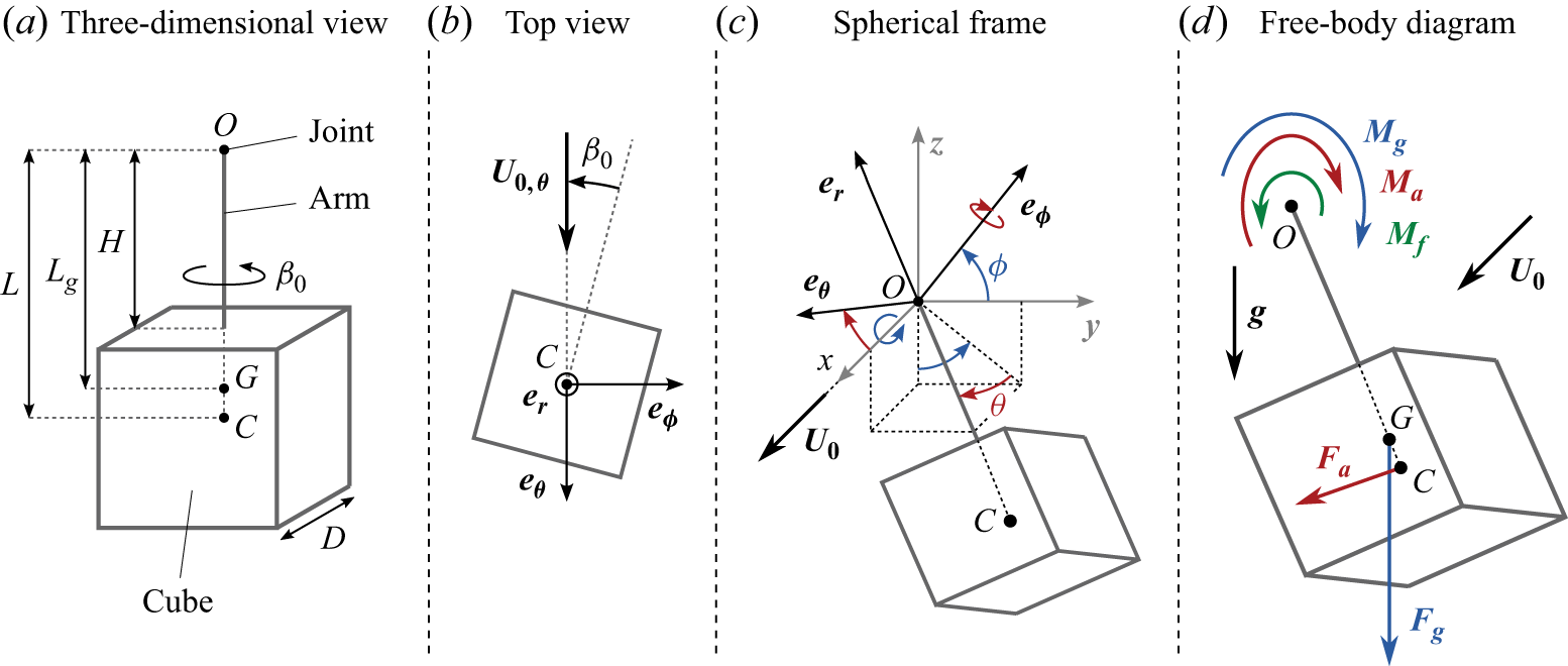
 β0
 U0,θ=(U0⋅eθ)eθ
 (er,eθ,eϕ)
 (x,y,z)
 Mf
 Ma
 Mg
 Fa
 Fg
 Fa

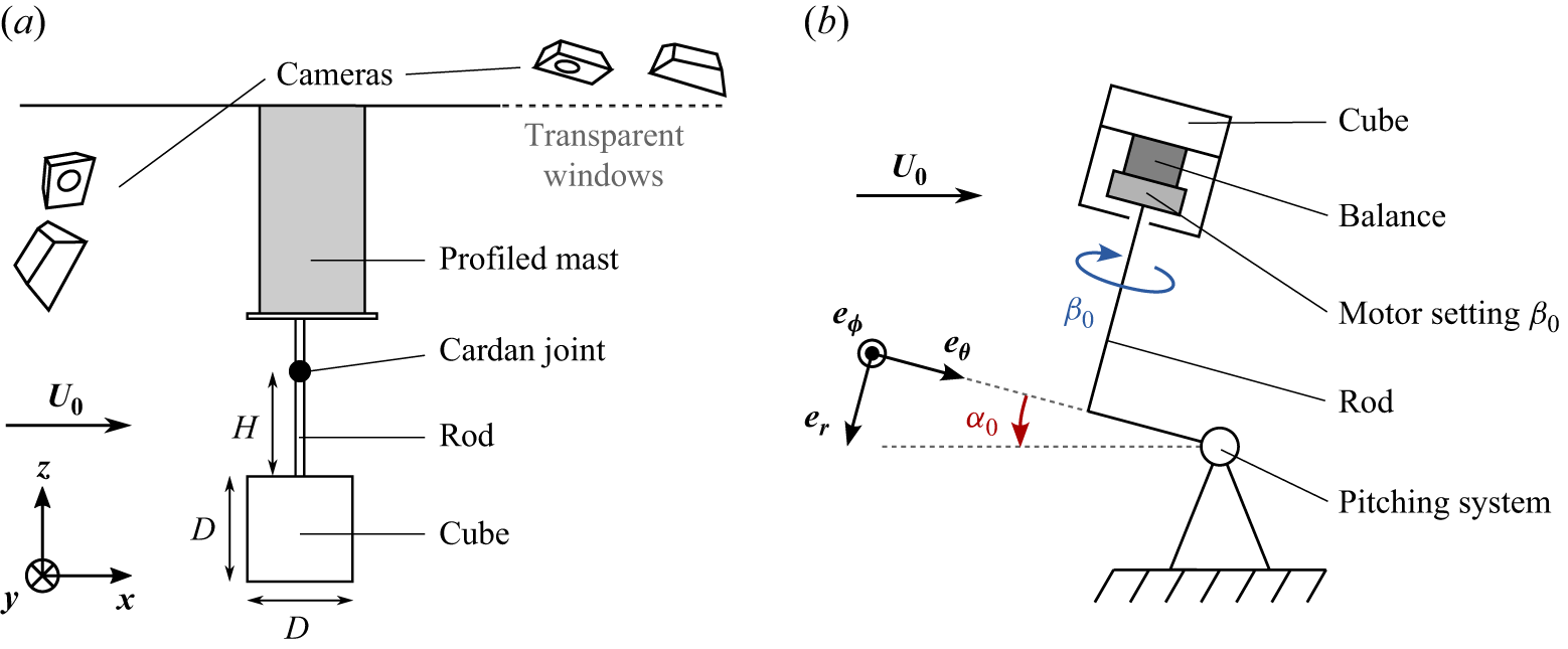

 (−θ,ϕ)
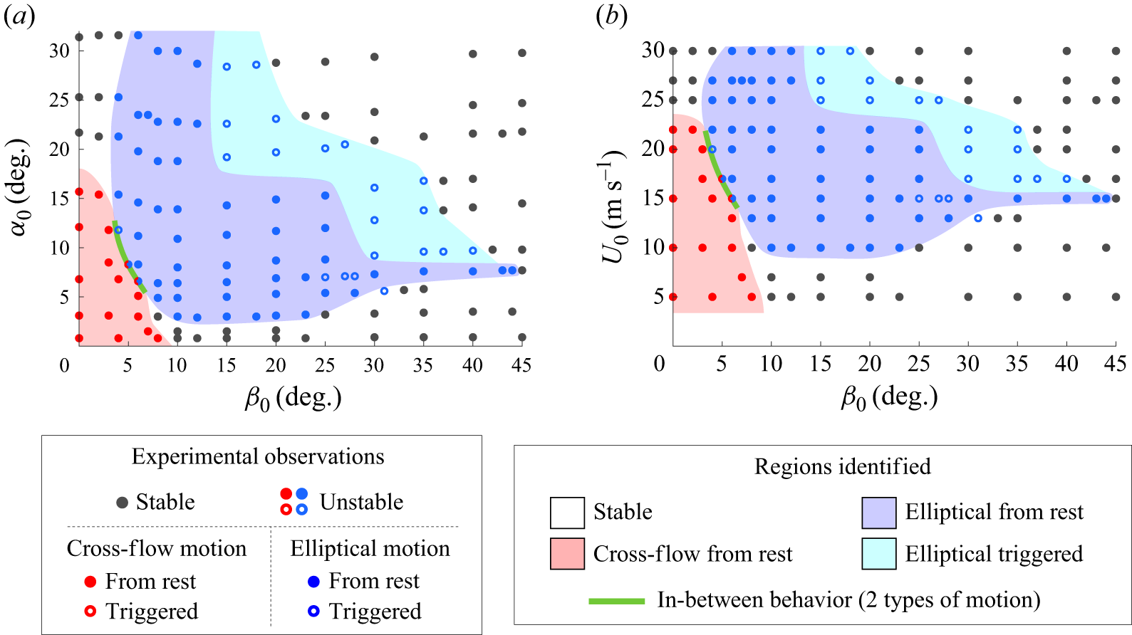
 (β0,α0)
 (β0,U0)
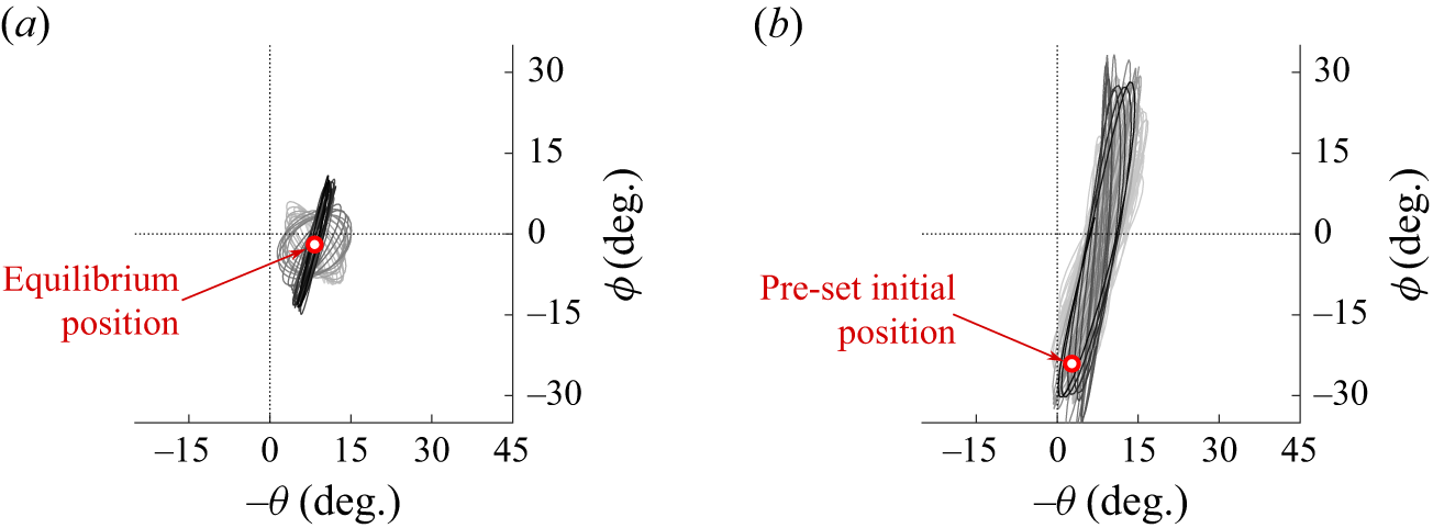
 β0=5∘
 U0=17m s−1
 (−θ,ϕ)

 cϕ
 cθ
 α
 β
 ∂cϕα
 ∂cϕβ
 ∂cθα
 ∂cθβ
 (β0,α0)
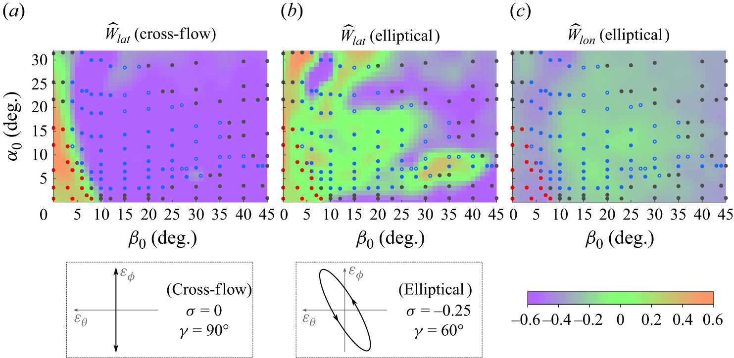
 W^lat
 (β0,α0)
 W^lat
 W^lon
 (β0,α0)
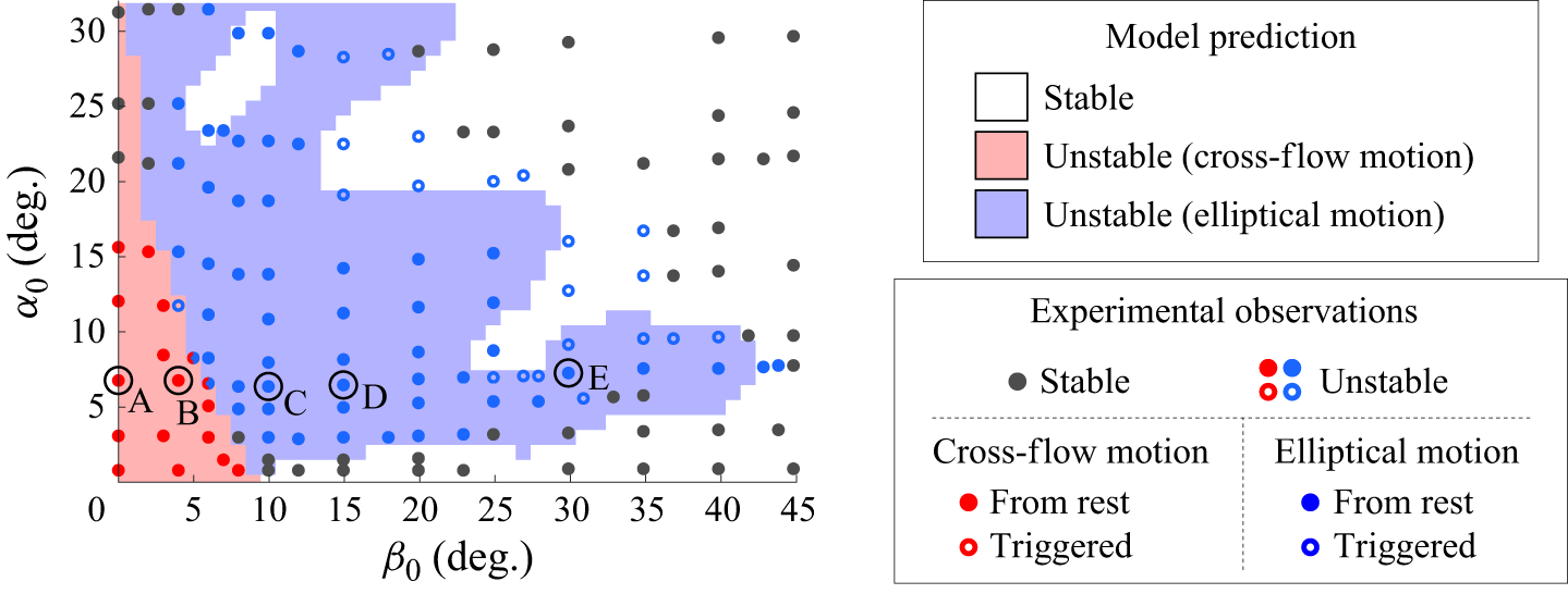
 W^lim=−0.3
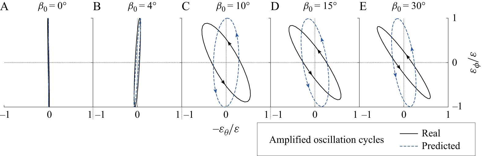
 (−εθ,εϕ)/ε
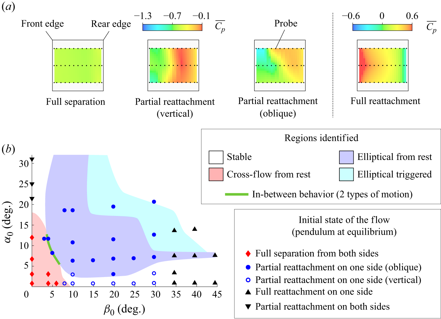
 Cp¯
 (β0,α0)
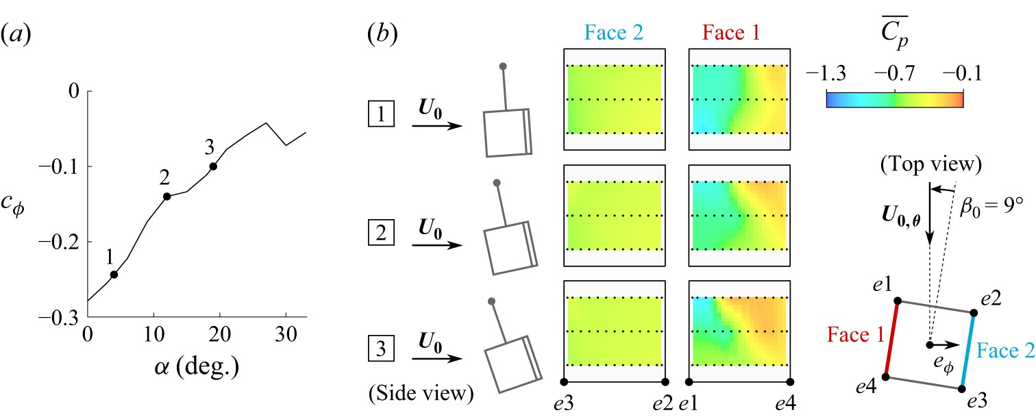
 cϕ
 α
 β0=9∘
 α
 U0,θ=(U0⋅eθ)eθ

 β0=10∘
 U0=15m s−1
 α
 β
 Cp~
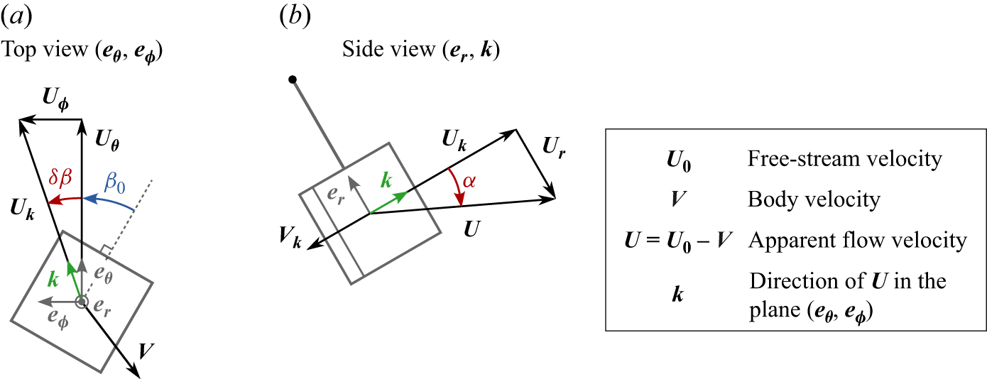
 β
 α
 Uθ=(U⋅eθ)eθ
 Uϕ=(U⋅eϕ)eϕ
 Ur=(U⋅er)er
 Uk=(U⋅k)k
 Vk=(V⋅k)k

 cϕ=Cϕ¯
 cθ=Cθ¯
 (β,α)

 95%
 |σ|≤0.4
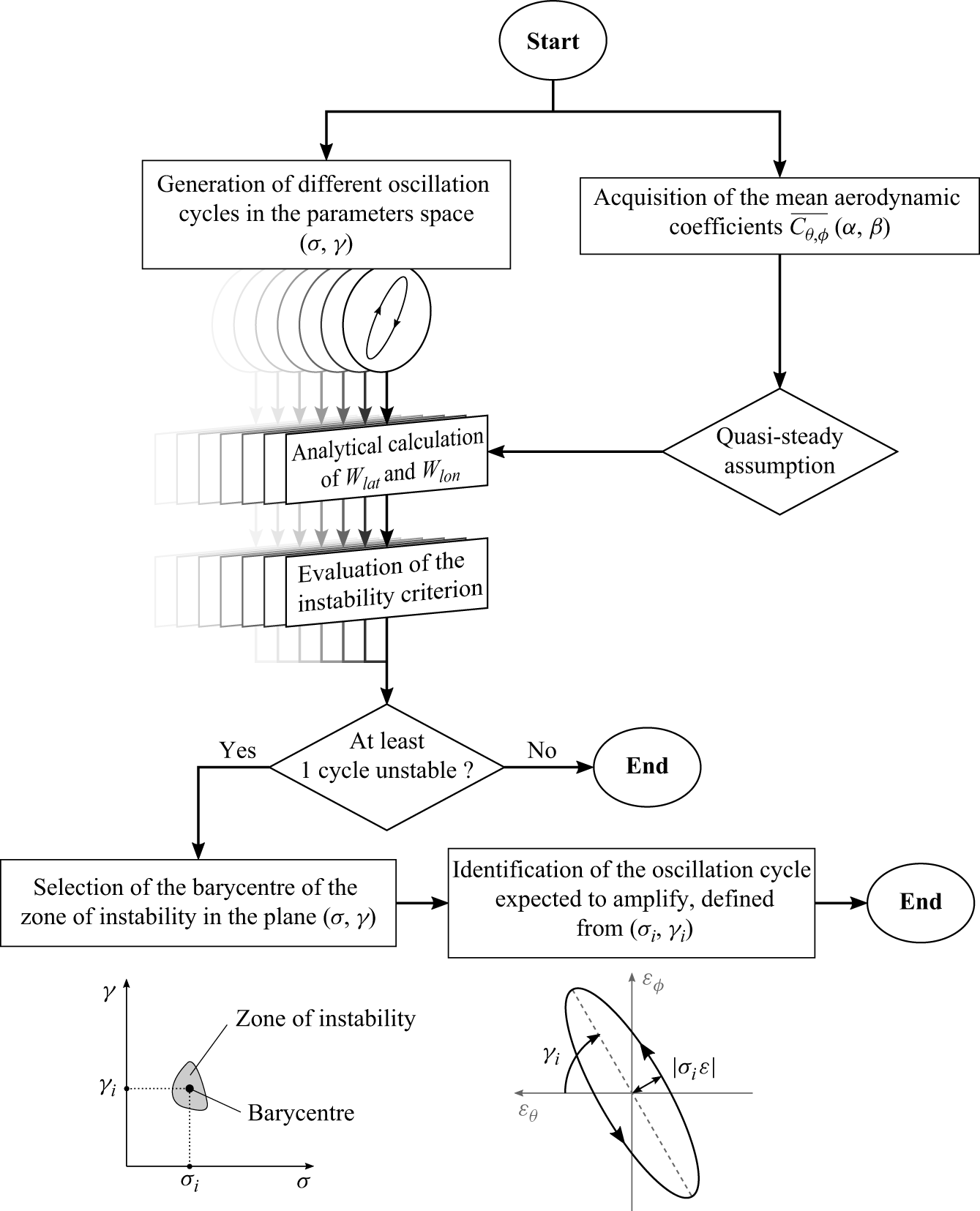
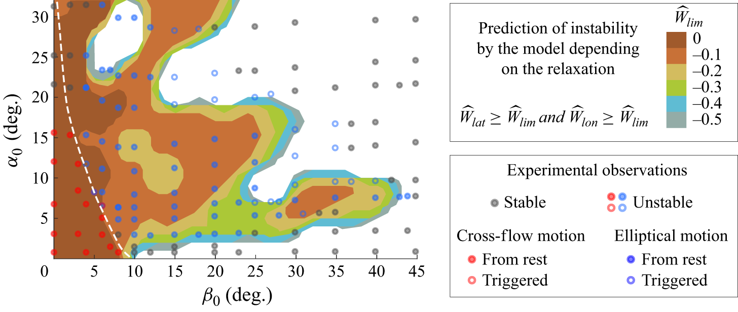
 W^lim
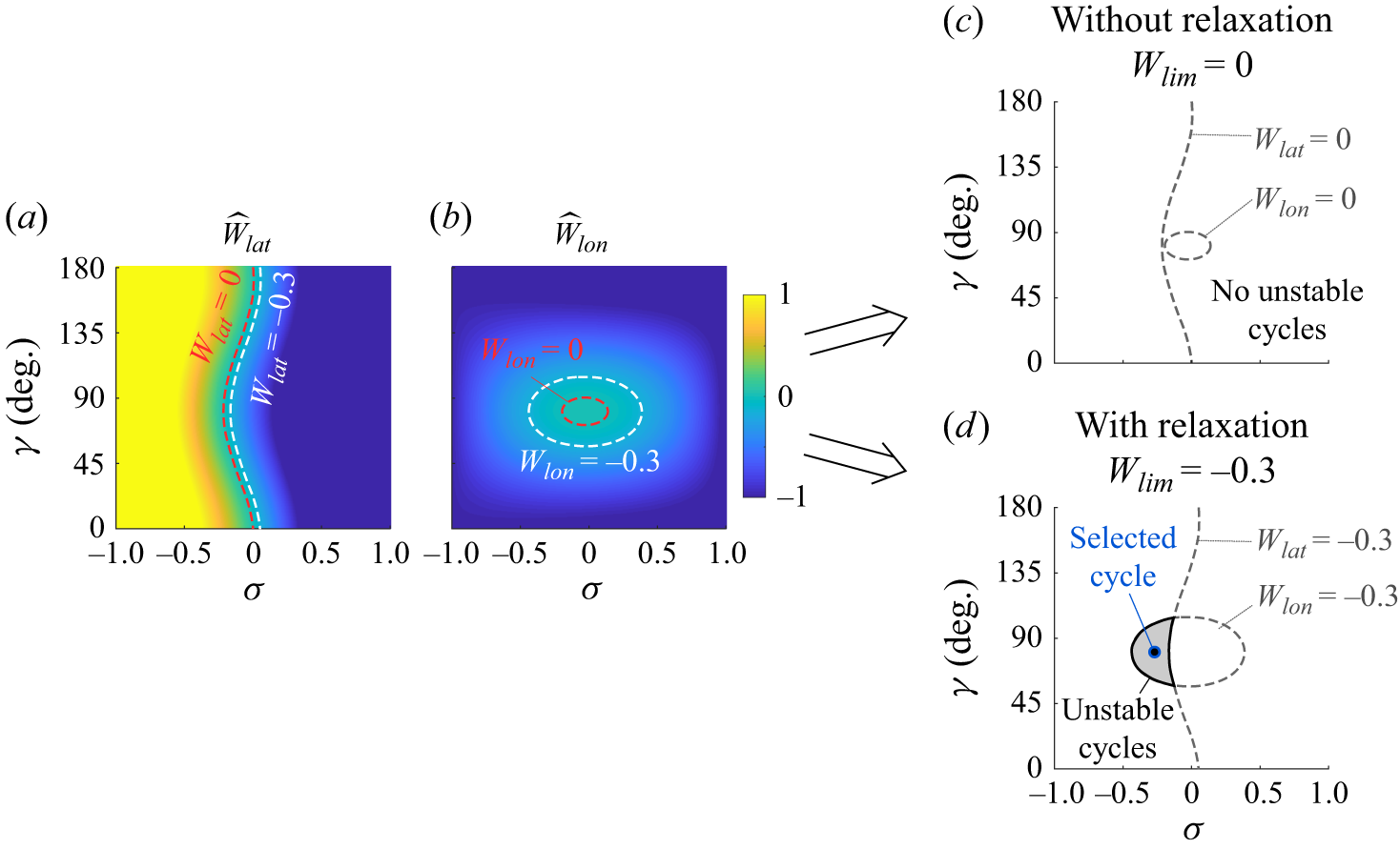
 W^lim=−0.3
 W^lim=0
 β0=15∘
 U0=15m s−1
 (σ,γ)
 W^lat
 W^lon
 W^lat,lon=W^lim
 W^lim


