1 INTRODUCTION
Inference after data-driven model selection is widely studied in both statistical and econometric literature.Footnote 1 It is now well known that widely used model-selection practices, such as pretesting, may have a large impact on the size properties of two-stage procedures and thus invalidate inference on the parameter of interest in the second stage. For the classical linear regression model with exogenous covariates, Kabaila (Reference Kabaila1995) and Leeb and Pötscher (Reference Leeb and Pötscher2005) show that confidence intervals (CIs) based on consistent model selection have a serious problem of under-coverage, while Andrews and Guggenberger (Reference Andrews and Guggenberger2009b) show that such CIs have asymptotic confidence size equal to 0. Furthermore, Andrews and Guggenberger (Reference Andrews and Guggenberger2009a) find extreme size distortion for the two-stage test after “conservative” model selection and propose various least favorable critical values (CVs).
In comparison, the literature on models that contain endogenous covariates, such as widely used instrumental variable (IV) regression models, remains relatively sparse. The uniform validity of post-selection inference for structural parameters in linear IV models with homoskedastic errors was studied by Guggenberger (Reference Guggenberger2010a), who advised not to use Hausman-type pretesting to select between ordinary least squares (OLS) and two-stage least squares (2SLS)-based t-tests because such two-stage procedures can be extremely over-sized with asymptotic CVs.Footnote 2 Instead, Guggenberger (Reference Guggenberger2010a) recommended to use the standard 2SLS-based t-test. However, the 2SLS-based t-test may exhibit undesirable size properties when the IVs are relatively weak. As such, in the quest for statistical power, many empirical practitioners still use pretesting in IV applications despite the important concern raised by Guggenberger (Reference Guggenberger2010a).Footnote 3
Recent surveys by Andrews, Stock, and Sun (Reference Andrews, Stock and Sun2019) and Lee et al. (Reference Lee, McCrary, Moreira and Porter2022) find that a considerable number of IV regressions in the American Economic Review (AER) report first-stage F-statistics below 10. Young (Reference Young2022) analyzes a sample of 1,359 empirical applications involving IV regressions in 31 papers published in the American Economic Association (AEA).Footnote 4 He also highlights that IVs often appear weak in these papers, so that inferences based on standard normal CVs can be unreliable, especially with heteroskedastic or clustered errors. Instead, Young (Reference Young2022) advocates the use of bootstrap methods based on their good performance in Monte Carlo simulations (but without theoretical justification). Furthermore, he argues that in these papers IV CIs almost always include OLS point estimates, and there is little statistical evidence of endogeneity and evidence that OLS is seriously biased, based on the low rejection rates of Hausman-type tests in his data.Footnote 5 Similarly, Keane and Neal (Reference Keane and Neal2024) argue that a rather strong IV is necessary to give high confidence that 2SLS will outperform OLS (e.g., with a first-stage F higher than 50, which is well above the industry standard of 10).
However, Young’s (Reference Young2022) finding from the AEA data that OLS estimates seem not to be very different from 2SLS estimates may be attributed to the fact that the used IVs are weak, so that 2SLS may be biased toward OLS, and Hausman-type tests also have low power in this case (see, e.g., Doko Tchatoka and Dufour, Reference Doko Tchatoka and Dufour2020, Reference Doko Tchatoka and Dufour2025). In particular, as shown by Guggenberger (Reference Guggenberger2010a), the Hausman test is not able to reject the null hypothesis of exogeneity when there is only a small degree of endogeneity, i.e., local endogeneity. Then, OLS-based inference is selected with high probability in the second stage. However, the OLS-based t-statistic often takes on very large values even under such local endogeneity, leading to severe size distortions. Such issues with pretesting for exogeneity are highly relevant to empirical practice, as endogeneity is mild in many IV applications. For example, Hansen, Hausman, and Newey (Reference Hansen, Hausman and Newey2008) report that the median, 75th quantile, and 90th quantile of estimated endogeneity parameters are only 0.279, 0.466, and 0.555, respectively, in their investigated AER, JPE, and QJE papers. Angrist and Kolesár (Reference Angrist and Kolesár2024) investigate three influential just-identified IV applications: Angrist and Krueger (Reference Angrist and Krueger1991), Angrist and Evans (Reference Angrist and Evans1998), and Angrist and Lavy (Reference Angrist and Lavy1999), and find that the estimated endogeneity is no more than 0.175, 0.075, and 0.460 for different specifications and samples in these papers, respectively.Footnote 6
Motivated by these issues, we study in this article the possibility of proposing a uniformly valid method for the two-stage testing procedure and a closely related Stein-type shrinkage procedure proposed by Hansen (Reference Hansen2017), and we consider an asymptotic framework under conditional heteroskedasticity or clustering, as allowing for non-homoskedastic errors is paramount for the methodology to be useful in practice. Given Young’s (Reference Young2022) recommendation to use bootstrap, we first examine the theoretical validity of bootstrapping the two procedures by obtaining the null limiting distributions of the bootstrap statistics and their associated asymptotic null rejection probabilities. Such (unconditional) asymptotic null rejection results are useful because even if the bootstrap cannot consistently estimate the distribution of interest conditional on the data (i.e., bootstrap invalidity in the usual sense), it may still be possible that the bootstrap test controls the asymptotic size and thus is valid unconditionally (see, e.g., Cavaliere and Georgiev, Reference Cavaliere and Georgiev2020 and the references therein). Here, we find that the standard wild bootstrap procedures are invalid both conditionally and unconditionally for the two-stage and shrinkage procedures even under strong IVs.Footnote 7 Furthermore, the usual intuition for bootstrapping Durbin–Wu–Hausman (DWH) tests is that one should restrict the bootstrap data-generating process (DGP) under exogeneity of the regressors. However, we find that such a bootstrap DGP can lead to extreme size distortion, with asymptotic null rejection probabilities approaching 1 in some settings. In contrast, the bootstrap DGP without this restriction typically exhibits much smaller asymptotic size distortions.Footnote 8
Second, to address the bootstrap failure under local endogeneity and provide uniformly valid inference, we propose a size-adjusted wild bootstrap procedure, which combines certain standard wild bootstrap CVs with an appropriate Bonferroni-based size-correction method, following the lead of McCloskey (Reference McCloskey2017). In addition, to accommodate weak identification, we propose a novel two-stage test statistic that adaptively switches between the OLS-based Wald statistic and the Anderson–Rubin (AR) weak-IV-robust statistic. The switching mechanism is based on a Hausman-type statistic for testing exogeneity, constructed under the null hypothesis that the structural parameter equals its unknown true value. This restriction ensures the validity of this exogeneity statistic even under weak identification. The resulting CVs are shown to be uniformly valid with heteroskedastic errors in the sense that they yield two-stage and shrinkage tests with correct asymptotic size. In particular, since standard wild bootstrap procedures cannot well mimic the key localized endogeneity parameter, specific attention is given to this parameter when designing the bootstrap DGP, and a Bonferroni-based size-correction technique is implemented to account for its presence in the limiting distributions of interest. Different from the conventional Bonferroni bound, which may lead to a conservative test with asymptotic size strictly less than the nominal level, the size-correction procedure always leads to a desirable asymptotic size. Finally, we extend the uniform validity result to clustered samples, in which case the rate of convergence of the estimators depends on the regressor, the instruments, the relative cluster size, and the intra-cluster correlation structure in a complicated way.
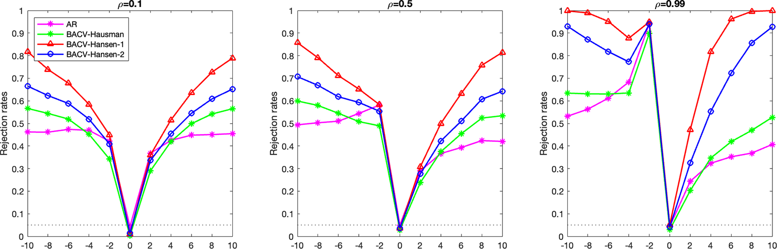
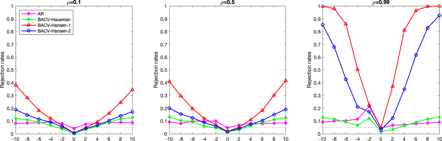
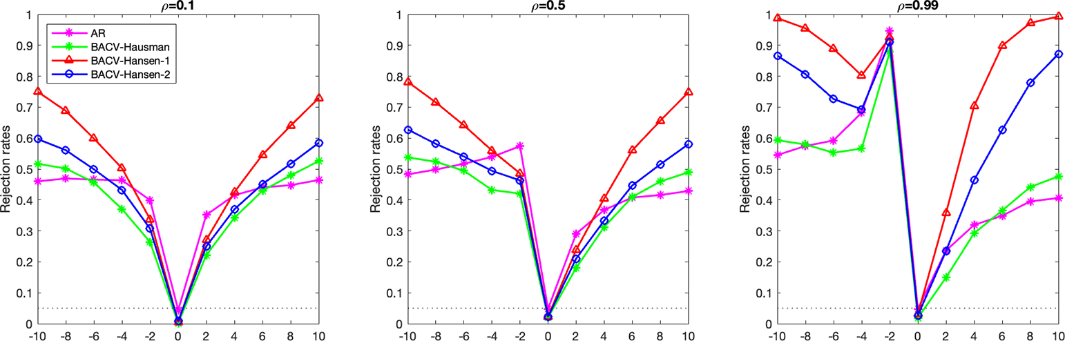
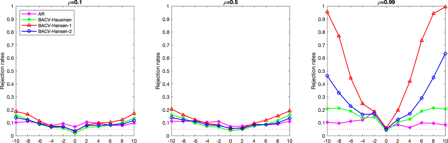
In terms of practical applications of our method, following the aforementioned studies by Hansen et al. (Reference Hansen, Hausman and Newey2008), Young (Reference Young2022), and Angrist and Kolesár (Reference Angrist and Kolesár2024), we are particularly interested in the IV settings where the values of endogeneity parameters are relatively small. In such cases, a pretest would typically fail to reject exogeneity, and the naive two-stage procedure could lead to severe size distortions. Our method circumvents this problem, allowing researchers to exploit the power advantage of the OLS-based test relative to IV approaches. More specifically, the proposed size-adjusted procedure is especially valuable when there is concern about potentially weak instruments: its power advantage is most pronounced in weak-IV scenarios, where weak-IV-robust methods maintain correct size but often suffer from relatively low power. Monte Carlo experiments confirm that our procedure achieves reliable size adjustment and remarkable power gains. We also note that the size-adjusted bootstrap Hansen-type shrinkage procedure tends to have superior finite-sample power performance than its Hausman-type counterpart. This may mainly be due to the relatively smooth transition between OLS and IV-based methods induced by the shrinkage approach.
The motivation for using bootstrap in the current testing problem stems from a growing literature showing that, when applied to IV models, well-designed bootstrap procedures typically provide superior inference than asymptotic approximations, including when IVs may be weak.Footnote 9 Furthermore, we are motivated by the literature showing the excellent performance of wild bootstrap methods with heteroskedastic or clustered errors.Footnote 10 Our size-correction procedure follows closely the seminal study by McCloskey (Reference McCloskey2017), who proposed Bonferroni-based size-correction procedures for general nonstandard testing problems, and McCloskey (Reference McCloskey2020) applied this method to inference in linear regression models after consistent model selection.Footnote 11
The remainder of this article is organized as follows. Section 2 presents the setting, test statistics, and parameter space of interest. Section 3 presents the main results of both standard and size-adjusted wild bootstrap methods. Section 4 investigates the finite sample power performance of our methods using simulations. Conclusions are drawn in Section 5. The proofs and further simulation results are provided in the Supplementary Material.
Throughout the article, for any positive integers n and m,
 $I_{n}$
and
 $0_{n \times m}$
stand for the
 $n \times n$
identity matrix and
 $n \times m$
zero matrix, respectively. For any full-column rank
 $n\times m$
matrix
 $A,\, P_A = A(A^{\prime }A)^{-1}A^{\prime }$
is the projection matrix on the space spanned by the columns of A, and
 $M_A = I_n-P_A.$
 $\lambda _{min}(A)$
denote the minimum eigenvalue of a square matrix A.
 $\|U\|$
denotes the usual Euclidean or Frobenius norm for a matrix
 $U.$
The usual orders of magnitude are denoted by
 $O_P(.)$
and
 $o_P(.)$
,
 $\rightarrow ^P$
stands for convergence in probability, while
 $\rightarrow ^d $
stands for convergence in distribution. We write
 $P^*$
to denote the probability measure induced by a bootstrap procedure conditional on the data, and
 $E^*$
and
 $Var^*$
to denote the expected value and variance with respect to
 $P^*$
. Following Gonçalves and White (Reference Gonçalves and White2004), for any bootstrap statistic
 $T^*$
, we write (1)
 $T^* \rightarrow ^{P^*} 0$
in probability P if for any
 $\delta> 0$
,
 $\epsilon>0$
,
 $lim_{n \rightarrow \infty } P[P^*(|T^*|>\delta )>\epsilon ] = 0$
, i.e.,
 $P^*(|T^*|>\delta ) = o_P(1)$
; (2)
 $T^* = O_{P^*} (n^\varphi )$
in probability P if and only if for any
 $\delta>0,$
there exists an
 $M_{\delta } < \infty $
such that
 $lim_{n \rightarrow \infty } P[P^*(|n^{-\varphi } T^* |>M_{\delta })>\delta ]=0$
, i.e., for any
 $\delta>0,$
there exists an
 $M_{\delta } < \infty $
such that
 $P^*(|n^{-\varphi } T^* |>M_{\delta })=o_P(1)$
; and (3)
 $T^* \rightarrow ^{d^*} T$
in probability P if, conditional on the data,
 $T^*$
weakly converges to T under
 $P^*$
, for all samples contained in a set with probability approaching one.
2 FRAMEWORK
2.1 Model and Test Statistics
We consider the following linear IV model:
 $$ \begin{align} y = X\theta + u, \quad X= Z \pi + v, \end{align} $$
where
 $y\in \mathbb {R}^n$
and
 $X\in \mathbb {R}^n$
are vectors of dependent and endogenous variables, respectively,
 $Z \in \mathbb {R}^{n \times k}$
is a matrix of instruments (
 $k \geq 1$
),
 $(\theta , \pi ')' \in \mathbb {R}^{k+1}$
are unknown parameters, and n is the sample size. Denote by
 $u_i$
,
 $v_i$
,
 $y_i$
,
 $X_i$
, and
 $Z_i$
the ith rows of u, v, y, X, and
 $Z,$
respectively, written as column vectors or scalars. For notational simplicity, we assume that the other exogenous variables have already been partialled out from the model.
The object of inferential interest is the structural parameter
 $\theta $
, and we consider the problem of testing the null hypothesis
 $H_0: \theta =\theta _0$
. We study the two-stage testing procedure for assessing
 $H_0$
, where an exogeneity test is conducted in the first stage to determine whether the OLS or IV-based method is appropriate for testing
 $H_0$
in the second stage. Assume that the instruments Z are exogenous, i.e.,
 $E_F[u_iZ_i]=0$
, where
 $E_F$
denotes expectation under the distribution
 $F.$
Under this orthogonality condition of the instruments, X is endogenous in (2.1) if and only if v and u are correlated. Consider the following linear projection of u on v:
 $$ \begin{align} u = v a + e, \; a = (E_F[v^2_i])^{-1} E_F[v_i u_i], \end{align} $$
where e is uncorrelated with v. Notice that the exogeneity of X in (2.1) can be assessed by testing the null hypothesis
 $H_a:\;a=0$
in (2.2). Substituting (2.2) into (2.1), we obtain
 $$ \begin{align} y = X \theta + v a + e, \end{align} $$
where X and v are uncorrelated with e. Therefore, the null hypothesis of exogeneity
 $H_{a}:\; a = 0$
can be assessed using a standard Wald statistic in the extended regression (2.3) (see, e.g., Doko Tchatoka and Dufour, Reference Doko Tchatoka and Dufour2014). To account for possible conditional heteroskedasticity, we consider the following control function-based Wald statisticFootnote
12
:
 $$ \begin{align} H_n = \hat{a}^2/\hat{V}_{a}, \end{align} $$
where
 $\hat {a} = (\tilde {v}' \tilde {v})^{-1} \tilde {v}' y$
,
 $\hat {V}_{a} = (n^{-1} \tilde {v}' \tilde {v})^{-1} \left ( n^{-2} \sum _{i=1}^n \tilde {v}^2_i \hat {e}^2_i \right ) (n^{-1} \tilde {v}'\tilde {v})^{-1}$
is the heteroskedasticity-robust estimator of the variance of
 $\hat {a}$
,
 $\tilde {v} = M_X \hat {v}$
,
 $\hat {v}=M_ZX,$
and
 $\hat {e}=M_{[X : \hat {v}]}y.$
Note that
 $\hat {e}$
is the residual vector from the OLS regression of y on X and
 $\hat {v}$
. If
 $\theta $
is strongly identified (Z being strong instruments) and X is exogenous,
 $H_n$
follows a
 $\chi ^2_{1}$
distribution asymptotically. The pretest rejects the null hypothesis that X is exogenous in (2.1) if
 $H_n>\chi ^2_{1, 1-\beta }$
, where
 $\chi ^2_{1, 1-\beta }$
is the
 $(1-\beta )$
th quantile of
 $\chi ^2_{1}$
-distributed random variable for some
 $\beta \in (0, 1)$
.
Let
 $\hat {\theta }_{2sls} = (X^{'}P_{Z}X)^{-1} X^{'}P_{Z}y,$
and
 $\hat {\theta }_{ols} = (X^{'}X)^{-1} X^{'} y$
be the 2SLS and OLS estimators of
 $\theta $
in (2.1), respectively. Also, define their corresponding variance estimators as
 $$ \begin{align} \hat{V}_{2sls} &= \left( n^{-1} X^{'}P_{Z}X \right)^{-1} \hat{\pi}' \left( n^{-2} \sum_{i=1}^n Z_i Z_i' \hat{u}^2_i(\hat{\theta}_{2sls}) \right) \hat{\pi} \left( n^{-1} X^{'}P_{Z}X \right)^{-1}, \notag \\ \hat{V}_{ols} &= \left( n^{-1}X^{'}X \right)^{-1} \left( n^{-2} \sum_{i=1}^n X_iX_i' \hat{u}^2_i(\hat{\theta}_{ols}) \right) \left( n^{-1}X^{'}X \right)^{-1}, \end{align} $$
where
 $\hat {u}_i(\hat {\theta }_{2sls}) = y_i - X_i \hat {\theta }_{2sls}$
,
 $\hat {u}_i(\hat {\theta }_{ols}) = y_i - X_i \hat {\theta }_{ols}$
, and
 $\hat {\pi } = (Z'Z)^{-1}Z'X$
. Then, the two-stage test statistic associated with the
 $H_n$
-based pretest of exogeneity in the first stage is given by

where
 $T_{ols}(\theta )$
and
 $T_{2sls}(\theta )$
are the Wald statistics with OLS and 2SLS estimates, respectively, i.e.,
 $$ \begin{align} T_{ols}(\theta) = ( \hat{\theta}_{ols} - \theta )^2 / \hat{V}_{ols}, \quad \text{and} \quad T_{2sls}(\theta) = ( \hat{\theta}_{2sls} - \theta )^2 / \hat{V}_{2sls}. \end{align} $$
Related to the two-stage procedure, Hansen (Reference Hansen2017) proposed a Stein-like shrinkage approach in the context of IV regressions. His estimator follows Maasoumi (Reference Maasoumi1978) in taking a weighted average of the 2SLS and OLS estimators, with the weight depending inversely on the test statistic for exogeneity, and the proposed shrinkage estimator is found to have substantially reduced finite-sample median squared error relative to the 2SLS estimator. Following Hansen’s (Reference Hansen2017) approach, we define the Stein-like shrinkage test statistic as follows:
 $$ \begin{align} T^S_{\tau,n}(\theta_0) = T_{ols}(\theta_0) w(H_n) + T_{2sls}(\theta_0) (1-w(H_n)), \end{align} $$
where the weight function takes the form
 $w(H_n) = \begin {cases} \tau / H_n \; \; \; \text {if} \; \; \; H_n \geq \tau \\ 1 \; \; \; \text {if} \; \; \; H_n < \tau \end {cases}$
, and
 $\tau $
is a shrinkage parameter chosen by the researcher. The shrinkage statistic has a relatively smooth transition between the OLS and 2SLS test statistics. In Section 4, we evaluate the performance of the shrinkage procedure with different choices of
 $\tau $
.
In addition, we define the weak-identification-robust version of the two-stage/shrinkage test statistics
 $T^S_{\beta ,n}(\theta _0)$
and
 $T^S_{\tau ,n}(\theta _0)$
. Specifically, we first propose the following weak-identification-robust version of
 $H_n$
by imposing
 $H_0: \theta = \theta _0$
:
 $$ \begin{align} H_n(\theta_0) = \hat{a}^2(\theta_0)/\hat{V}_{a}(\theta_0), \end{align} $$
where
 $\hat {a}(\theta _0) = (\hat {v}' \hat {v})^{-1} \hat {v}' \tilde {y}(\theta _0)$
,
 $\hat {V}_{a}(\theta _0) = (n^{-1} \hat {v}' \hat {v})^{-1} \left ( n^{-2} \sum _{i=1}^n \hat {v}^2_i \tilde {e}^2_i(\theta _0) \right ) (n^{-1} \hat {v}'\hat {v})^{-1}$
is the (null-imposed) heteroskedasticity-robust estimator of the variance of
 $\hat {a}(\theta _0)$
,
 $\tilde {y}(\theta _0) = y - X \theta _0$
,
 $\hat {v}=M_ZX,$
and
 $\tilde {e}(\theta _0)=M_{\hat {v}}\tilde {y}(\theta _0)$
. Note that
 $\tilde {e}(\theta _0)$
is the residual vector from the OLS regression of
 $\tilde {y}(\theta _0)$
on
 $\hat {v}$
. When
 $H_0$
is true, and X is exogenous (i.e.,
 $a=0$
),
 $H_n(\theta _0)$
follows a
 $\chi ^2_{1}$
distribution asymptotically, no matter whether the IVs are strong or weak.Footnote
13
Now, let us define the heteroskedasticity-robust AR statistic as
 $$ \begin{align} T_{ar}(\theta_0) = \left( n^{-1/2} \tilde{y}(\theta_0)'Z \right) \left( \hat{V}_{ar}(\theta_0) \right)^{-1} \left( n^{-1/2} Z'\tilde{y}(\theta_0) \right), \end{align} $$
where
 $\hat {V}_{ar}(\theta _0) = n^{-1} \sum _{i=1}^n Z_iZ_i' \tilde {y}^2_i(\theta _0)$
. Then, the weak-IV-robust two-stage/shrinkage test statistics associated with the
 $H_n(\theta _0)$
pretest statistic are given by

2.2 Parameter Space and Asymptotic Size
Assume that
 $\{(u_i, v_i, Z_i): i\leq n\}$
in (2.1) are i.i.d. with distribution F. To characterize the asymptotic size of the two-stage and shrinkage tests, we define the parameter space
 $\Gamma $
of the nuisance parameter vector
 $\gamma $
following the seminal studies by Andrews and Guggenberger (Reference Andrews and Guggenberger2009a, Reference Andrews and Guggenberger2009b, Reference Andrews and Guggenberger2010a, Reference Andrews and Guggenberger2010b), Guggenberger (Reference Guggenberger2012), and Guggenberger and Kumar (Reference Guggenberger and Kumar2012). For the current testing problem, define the vector of nuisance parameters
 $\gamma = (\gamma _1, \gamma _2, \gamma _3)$
by
 $$ \begin{align} \gamma_1 = a, \;\; \gamma_2 = (\gamma_{21},\gamma_{22},\gamma_{23},\gamma_{24},\gamma_{25}),\;\; \gamma_3 = F, \end{align} $$
where a is defined in (2.2),
 $\gamma _{21}=\pi , \gamma _{22}=E_Fe_i^2Z_iZ_i', \gamma _{23}=E_Fe^2_iv_i^2, \gamma _{24}= E_F Z_i Z^{\prime }_i,$
and
 $\gamma _{25}=E_F v_i^2$
. Here,
 $\gamma _1$
measures the degree of endogeneity of X and is the key parameter in the current testing problem, as it determines the point of discontinuity of the null limiting distributions of the two-stage and shrinkage test statistics. For the parameter space, let
 $$ \begin{align} \Gamma_1= \mathbb{R}, \;\; \Gamma_2 & = \Big\{(\gamma_{21},\gamma_{22},\gamma_{23},\gamma_{24},\gamma_{25}): \gamma_{21}=\pi_n \in \mathbb{R}^k, \gamma_{22}=E_Fe_i^2Z_iZ_i' \in \mathbb{R}^{k \times k}, \Big. \notag \\ &\quad \gamma_{23}=E_Fe^2_iv_i^2 \in \mathbb{R}, \gamma_{24}= E_F Z_i Z^{\prime}_i \in \mathbb{R}^{k \times k}, \gamma_{25}= E_F v_i^2 \in \mathbb{R}, \Big. \notag \\ &\quad\textit{s.t.}\;\; \lambda_{min}(\gamma_{22}) \geq \underline{\kappa}, \gamma_{23}> 0, \lambda_{min}(\gamma_{24}) \geq \underline{\kappa}, \; \text{and} \; \gamma_{25} > 0 \Big\}, \end{align} $$
for some
 $\underline {\kappa }>0 $
that does not depend on n. We note that the current framework allows for weak identification. In addition,
 $\Gamma _3(\gamma _1, \gamma _2)$
is defined as follows:
 $$ \begin{align} \Gamma_3(\gamma_1, \gamma_2) &= \Big\{ F: \; E_F e_i v_i = E_F e_i Z_i = E_F v_i Z_i = 0,\; \notag \\ & \quad E_F e_i^2 v_i Z_i = E_F e_i v_i^2 Z_i = E_F e_iv_i Z_i Z_i' =0,\; \Big. \notag \\ & \quad E_Fv_i^2Z_iZ_i' \in \mathbb{R}^{k \times k} \;\; \text{with} \;\; \lambda_{min}(E_Fv_i^2Z_iZ_i') \geq M^{-1}, \; \Big. \\ & \quad \left\lVert E_F \left( ||Z_i e_i||^{2+\xi}, ||Z_iv_i||^{2+\xi}, |v_ie_i|^{2+\xi}, ||Z_iZ_i'||^{2+\xi}, |X_i|^{2(2+\xi)} \right)'\right\rVert \leq M \Big\},\notag \end{align} $$
for some constant
 $\xi> 0$
and
 $M<\infty $
. We then define the whole nuisance parameter space
 $\Gamma $
of
 $\gamma $
as
 $$ \begin{align} \Gamma = \{ \gamma = (\gamma_1, \gamma_2, \gamma_3): \gamma_1 \in \Gamma_1, \gamma_2 \in \Gamma_2, \gamma_3 \in \Gamma_3(\gamma_1, \gamma_2)\}, \end{align} $$
where
 $\Gamma _j,\;j=1,2,3$
are given in (2.13) and (2.14). This nuisance parameter space extends the one defined in Guggenberger (Reference Guggenberger2010a) to allow for conditional heteroskedasticity and is similar to those defined in Guggenberger (Reference Guggenberger2012) and Guggenberger and Kumar (Reference Guggenberger and Kumar2012), which also allow for heteroskedastic errors. In Section 3.3, we further extend the analysis to the case with clustered data and show that our size-adjusted wild bootstrap is also uniformly valid in that case. The condition that
 $E_F e_i^2 v_i Z_i = E_F e_i v_i^2 Z_i = E_F e_iv_i Z_i Z_i' =0$
in (2.14) is similar to that imposed for
 $\Gamma _3(\gamma _1, \gamma _2)$
in Guggenberger (Reference Guggenberger2010a).Footnote
14
Now, we define the asymptotic size. Let
 $T_n(\theta _0)$
denote a generic test statistic. Let
 $c_n$
denote a (possibly data-dependent) CV being used for the two-stage testing or shrinkage procedure. Then, the finite sample null rejection probability (NRP) of
 $T_n(\theta _0)$
evaluated at
 $\gamma \in \Gamma $
is given by
 $P_{\theta _0, \gamma }\left [ T_{n} (\theta _0)> c_n\right ]$
, where
 $P_{\theta _0, \gamma } \left [ E_n \right ]$
denotes the probability of event
 $E_n$
when
 $\theta _0$
and
 $\gamma $
are the true values of the parameters. Then, the asymptotic NRP of the test evaluated at
 $\gamma \in \Gamma $
is given by
 $\underset {n \rightarrow \infty }{lim sup} P_{\theta _0, \gamma } \left [T_{n} (\theta _0)> c_n\right ]$
, while the asymptotic size is given by
 $$ \begin{align} AsySz[c_n] = \underset{n \rightarrow \infty}{lim sup} \underset{\gamma \in \Gamma}{sup} P_{\theta_0, \gamma} \left[ T_{n} (\theta_0)> c_n \right]. \end{align} $$
In general, asymptotic NRP evaluated at a given
 $\gamma \in \Gamma $
is not equal to the asymptotic size of the test. To control the asymptotic size, one needs to control the null limiting behavior of
 $T_{n}(\theta _0)$
under drifting parameter sequences
 $\{ \gamma _n: n \geq 1\}$
indexed by the sample size (see, e.g., Andrews and Guggenberger, Reference Andrews and Guggenberger2009a, Reference Andrews and Guggenberger2009b, Reference Andrews and Guggenberger2010a, Reference Andrews and Guggenberger2010b, Guggenberger, Reference Guggenberger2012, and Guggenberger and Kumar, Reference Guggenberger and Kumar2012).
Following the arguments used in these papers, to derive
 $AsySz[c_n],$
we can study the asymptotic NRP along certain parameter sequences of the type
 $\{\gamma _{n,h}\}$
(defined below) for some
 $h\in \mathscr {H}$
, as the highest asymptotic NRP is materialized under such a sequence, where
 $$ \begin{align} \mathscr{H} &= \Bigg\{ h = (h_1, h^{\prime}_{21},vec(h_{22})', h_{23},vec(h_{24})', h_{25})' \in \mathbb{R}^{2k^2+k+3}_{\infty}: \notag \\ & \quad \exists \{\gamma_n = (\gamma_{n,1}, \gamma_{n,2}, \gamma_{n,3}) \in \Gamma: n \geq 1\} \quad s.t. \Big.\notag\\ &\quad n^{1/2}\gamma_{n,1} \rightarrow h_1 \in \mathbb{R}_{\infty},\;\;\gamma_{n,2} \rightarrow h_2=(h_{21},h_{22}, h_{23},h_{24},h_{25}), \; \lambda_{min}(A)\geq \underline{\kappa} \Big.\notag\\ & \;\;\;\; \text{for}\;\;A\in \{ h_{22}, h_{24}\}, \; h_{23}>0, \; h_{25}>0 \Bigg\} \end{align} $$
for some
 $\underline {\kappa }>0$
and
 $\mathbb {R}_{\infty } = \mathbb {R} \cup \{ \pm \infty \}.$
Then, for
 $h \in \mathscr {H}$
, the relevant sequence of parameters
 $\{\gamma _{n,h}\} \subset \Gamma $
is defined following Guggenberger (Reference Guggenberger2010a) as
 $\gamma _{n,h} = ( \gamma _{n,h,1}, \gamma _{n,h,2}, \gamma _{n,h,3} ),$
where
 $$ \begin{align} \gamma_{n,h,1} = (E_{F_n}[v^2_i])^{-1} E_{F_n}[v_i u_i], \;\; \gamma_{n,h,2} = (\gamma_{n,h,21} ,\gamma_{n,h,22} , \gamma_{n,h,23} ,\gamma_{n,h,24}, \gamma_{n,h,25}), \end{align} $$
with
 $\gamma _{n,h,21}=\pi _n$
,
 $\gamma _{n,h,22}=E_{F_n}e_i^2Z_iZ_i'$
,
 $\gamma _{n,h,23}=E_{F_n}e^2_iv_i^2, \gamma _{n,h,24}= E_{F_n} Z_i Z^{\prime }_i$
,
 $\gamma _{n,h,25}=E_{F_n} v_i^2$
, s.t.
 $$ \begin{align} n^{1/2}\gamma_{n,h,1} \rightarrow h_1, \; \gamma_{n,h,2} \rightarrow h_2, \; \text{and} \; \gamma_{n,h,3} = F_n\in \Gamma_3(\gamma_{n,h,1}, \gamma_{n,h,2}). \end{align} $$
More specifically, under
 $\{ \gamma _{n,h} \}$
satisfying (2.19) with
 $|h_1| = \infty $
(i.e., strong endogeneity),
 $H_n \rightarrow ^P \infty $
, and the two-stage and shrinkage test statistics
 $T_{l,n}^S(\theta _0)$
,
 $l \in \{\beta , \tau \}$
, are asymptotically equivalent to the 2SLS-based t-statistic. On the other hand, under
 $\{\gamma _{n,h}\}$
satisfying (2.19) with
 $|h_1| < \infty $
(i.e., local endogeneity) and
 $||h_{21}|| \geq \kappa $
, where
 $\kappa> 0$
(i.e., strong IVs), the following joint convergence results hold for the two-stage and shrinkage statistics
 $T^S_{l,n}(\theta _0)$
for
 $l \in \{\beta ,\tau \}$
,
 $$ \begin{align} \begin{pmatrix} T^S_{\beta,n}(\theta_0) \\ T^S_{\tau,n}(\theta_0) \end{pmatrix} & \rightarrow^{d} \begin{pmatrix} \tilde{T}^S_{\beta,h} \\ \tilde{T}^S_{\tau,h} \end{pmatrix}, \end{align} $$
where

 $\eta ^S_{1,h}\sim \chi ^2_{1}$
,
 $\eta ^S_{2,h}\sim \chi ^2_1 \Big ( (h^{\prime }_{21} h_{22}h_{21} + h_{23} )^{-1} h^2_{25} h^2_1 \Big )$
, and
 $\eta ^S_{3,h}\sim \chi ^2_1 \Big (\big (\frac { h^{\prime }_{21} h_{22} h_{21}}{(h^{\prime }_{21} h_{24}h_{21})^{2}} + h_{23} h_{25}^{-2} \big )^{-1}h^2_1\Big )$
.Footnote
15
Furthermore, the following joint convergence results hold for
 $T^W_{l,n}(\theta _0)$
for
 $l \in \{\beta ,\tau \}$
under local endogeneity, no matter whether IVs are strong or weak (as both
 $H_n(\theta _0)$
and
 $T_{ar}(\theta _0)$
are weak-identification-robust):
 $$ \begin{align} \begin{pmatrix} T^W_{\beta,n}(\theta_0) \\ T^W_{\tau,n}(\theta_0) \end{pmatrix} & \rightarrow^{d} \begin{pmatrix} \tilde{T}^W_{\beta,h} \\ \tilde{T}^W_{\tau,h} \end{pmatrix}, \end{align} $$
where

 $\eta ^W_{1,h} \sim \chi ^2_{k}$
,
 $\eta ^W_{2,h} = \eta ^S_{2,h}$
, and
 $\eta ^W_{3,h}\sim \chi ^2_1 \Big ( h_{23}^{-1} h_{25}^2 h_1^2 \Big )$
.
In the next section, we will study the asymptotic behaviors of the two-stage and shrinkage tests under bootstrap-based CVs.
3 MAIN RESULTS
3.1 Standard Wild Bootstrap
In this section, we study the asymptotic behavior of the standard wild bootstrap for the two-stage testing and shrinkage procedures.
Wild Bootstrap Algorithm:
-
1. Compute the (null-restricted) residuals from the first-stage and structural equations:
 $\hat {v} = X -Z \hat {\pi }$
,
$\hat {u}(\theta _0) = y - X \theta _0$
, where
$\hat {\pi }=(Z^{\prime }Z)^{-1}Z^{\prime }X$
denotes the least squares estimator of
$\pi $
.
-
2. Generate the bootstrap pseudo-data following
$X^{\ast } = Z \hat {\pi } + v^{\ast }, y^{\ast } = X^{\ast }\theta _0 + u^{\ast },$
where there are two options to generate the bootstrap disturbances:-
(a)
$v^{\ast }$
and
$u^{\ast }$
are generated independently from each other. Specifically, in the current case with heteroskedastic data, we set for each observation i:
$v^*_i = \hat {v}_i \omega ^*_{1i},$
and
$u^*_i = \hat {u}_i(\theta _0) \omega ^*_{2i}$
, where
$\omega ^*_{1i}$
and
$\omega ^*_{2i}$
are two random variables with mean 0 and variance
$1$
, i.e.,
$E^*\left [\omega ^*_{1i}\right ]=E^*\left [\omega ^*_{2i}\right ]=0$
and
$Var^*\left [\omega ^*_{1i}\right ]=Var^*\left [\omega ^*_{2i}\right ]=1$
, and they are independent from the data and independent from each other. -
(b)
$v^{\ast }$
and
$u^{\ast }$
are drawn dependently from each other. We set for each observation i:
$v^*_i = \hat {v}_i \omega ^*_{1i} $
, and
$u^*_i = \hat {u}_i(\theta _0) \omega ^*_{1i}$
.
Following Young (Reference Young2022), we refer to (a) as independent transformation of disturbances and (b) as dependent transformation of disturbances.Footnote 16
-
-
3. Compute the bootstrap analogs of the two-stage and shrinkage test statistics:
(3.1)where
$T^*_{ols}(\theta _0)$
,
$T^*_{2sls}(\theta _0)$
,
$T^*_{ar}(\theta _0)$
,
$H^*_n$
, and
$H^*_n(\theta _0)$
are bootstrap analogs of
$T_{ols}(\theta _0)$
,
$T_{2sls}(\theta _0)$
,
$T_{ar}(\theta _0)$
,
$H_n$
, and
$H_n(\theta _0)$
, respectively, which are obtained from the bootstrap samples generated in Step 2.
-
4. For
$l \in \{\beta ,\tau \}$
and
$s \in \{S, W \}$
, repeat Steps 2 and 3 B times and obtain
$\{ T^{s*(b)}_{l,n}(\theta _0), b=1, \ldots , B \}$
. The bootstrap test with the test statistic
$T^s_{l,n}(\theta _0)$
rejects
$H_0$
if the corresponding bootstrap p-value is less than the nominal level
$\alpha .$





 is less than the nominal level

Following the standard arguments for bootstrap validity, to check whether (conditional on the data) the bootstrap can consistently estimate the distribution of the two-stage or shrinkage test statistic, one needs to check whether under
 $H_0$
and both cases of strong endogeneity (
 $|h_1|=\infty $
) and local endogeneity (
 $|h_1| < \infty $
),
 $ \sup _{x \in \mathbb {R}} \left | P^*\left (T^{s*}_{l,n}(\theta _0) \leq x \right ) - P\left (T^s_{l,n}(\theta _0) \leq x\right ) \right | \rightarrow ^P 0, $
for
 $l \in \{\beta ,\tau \}$
and
 $s \in \{S, W\}$
. However, we note below that neither bootstrap procedure consistently estimates the distribution of interest under local endogeneity, even with strong IVs (i.e., even when
 $|| \gamma _{21} ||> 0$
).
More specifically, it holds for the bootstrap statistics with dependent or independent transformation (for the dependent transformation, we further require
 $E^*\left [\omega _{1i}^{*3} \right ]=0$
and
 $E^*\left [\omega _{1i}^{*4}\right ] =1$
; see Lemma S.5 in the Supplementary Material for details) that
 $$ \begin{align} n^{-1/2}\begin{pmatrix} Z^{'}u^* \\ \left(u^{*'}v^* - E^*[u^{*'}v^*]\right) \end{pmatrix} \rightarrow^{d^*} \begin{pmatrix} \psi^*_{Ze} \\ \psi^*_{ve} \end{pmatrix}, \end{align} $$
in probability P (i.e., with probability approaching one according to P), where the bootstrap (conditional) weak limit
 $(\psi ^{*'}_{Ze}, \psi ^*_{ve})'$
is the same as
 $(\psi ^{\prime }_{Ze}, \psi _{ve})'$
, i.e., the weak limit of
 $n^{-1/2} \left ( (Z'u)', (u'v - E_F[u'v]) \right )'$
. Therefore, the bootstrap procedures do replicate well the randomness in the original sample.
By contrast, under local endogeneity, the standard wild bootstrap does not well mimic the key localization parameter
 $h_1$
, leading to a discrepancy between the original and bootstrap samples. In particular, let
 $h^b_1$
denote the localization parameter of endogeneity in the bootstrap world, then we have:
-
1.
$h^b_1=0$
for the bootstrap with independent transformation. This is because the random weights
$\omega ^*_{1i}$
and
$\omega ^*_{2i}$
under this transformation are independent from each other. As a consequence, the bootstrap disturbances
$u^*_i$
and
$v^*_i$
are independent from each other (conditional on the data), which implies that
$E^*[u_i^* v_i^*] = E^*[\hat {u}_i(\theta _0) \omega _{1i}^* \hat {v}_i \omega _{2i}^*] = \hat {u}_i(\theta _0) \hat {v}_i E^*[\omega _{1i}^*] E^*[\omega _{2i}^*] = 0$
. -
2.
$h^b_1 = h_1 + h_{25}^{-1} \psi _{ve}$
for the one with dependent transformation, where
$\psi _{ve} \sim N(0, h_{23})$
. This is due to the fact that the same random weight
$\omega ^*_{1i}$
is used to generate the bootstrap disturbances
$u^*_i$
and
$v^*_i$
, so that
$E^*[u_i^* v_i^*] = E^*[\hat {u}_i(\theta _0) \omega _{1i}^* \hat {v}_i \omega _{1i}^*] = \hat {u}_i(\theta _0) \hat {v}_i E^*[\omega _{1i}^{*2}] = \hat {u}_i(\theta _0) \hat {v}_i$
. Intuitively, while the bootstrap with dependent transformation can mimic the situation of local endogeneity in the original sample (
$h^b_1$
is finite with probability approaching one when
$h_1$
is finite), the approximation is imprecise and results in an extra error term
$h_{25}^{-1}\psi _{ve}$
, whose value depends on the actual realization of the sample (e.g., see Theorems S.1 and S.2 in the Supplementary Material for details).


However, even if the bootstrap is inconsistent conditional on the data, it may still be valid in the unconditional sense (see, e.g., Cavaliere and Georgiev, Reference Cavaliere and Georgiev2020 and the references therein). More precisely, the bootstrap might still be able to provide a valid test in the current context if its asymptotic NRP does not exceed the nominal level
 $\alpha $
under any parameter sequence
 $\{ \gamma _{n,h} \}$
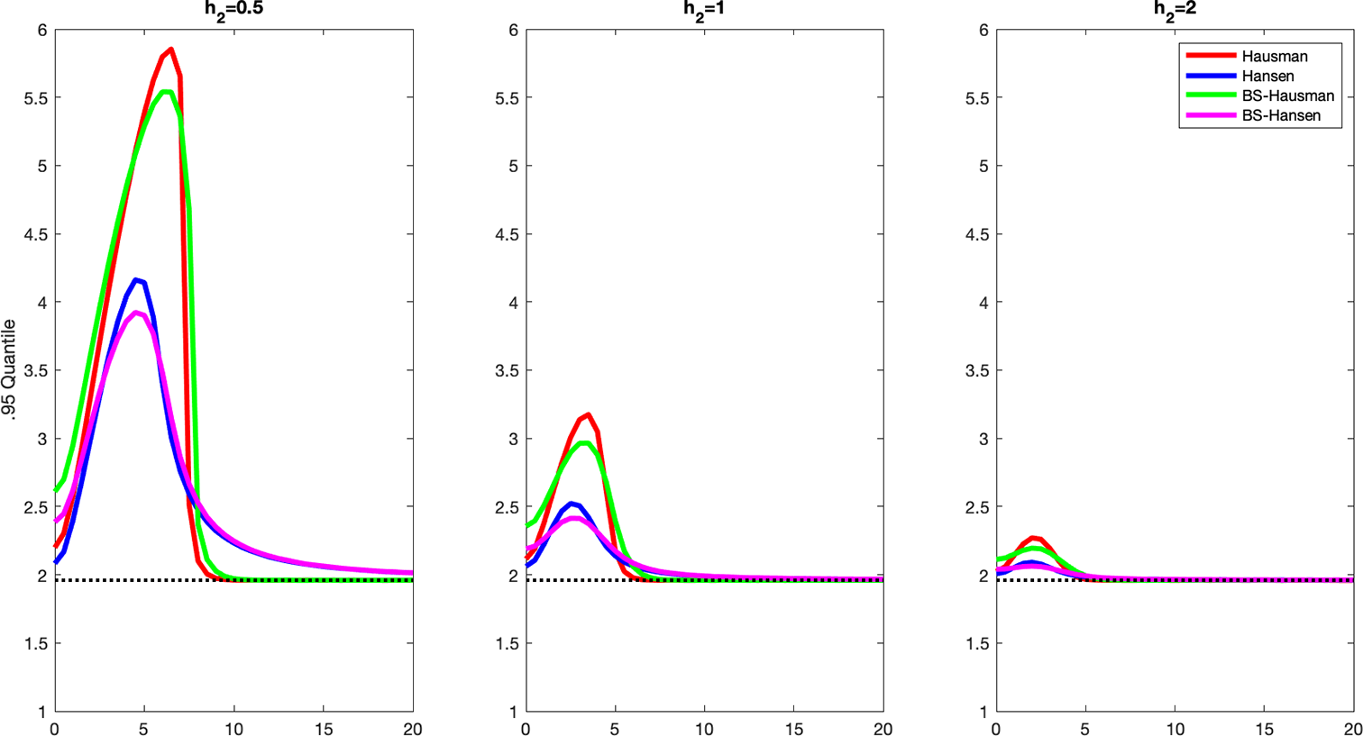
in (2.19). To further shed light on the behavior of bootstrap statistics with the dependent transformation, we apply the results in (2.20) and (2.21) and Theorems S.1 and S.2 in the Supplementary Material to plot the quantiles of the null limiting distributions of the original and bootstrap test statistics for the case of strong identification and conditional homoskedasticity studied in Guggenberger (Reference Guggenberger2010a). The limiting distributions of both the two-stage and shrinkage test statistics are substantially simplified in this case and depend on only two scalar parameters, say,
 $h_{1,ho}$
and
 $h_{2,ho}$
.
 $h_{1,ho}$
captures the degree of local endogeneity and
 $h_{2,ho}$
captures the IV strength, respectively.Footnote
17
Figure 1 reports the 95% quantiles of
 $\tilde {T}^S_{l,h}$
defined in (2.20) and its bootstrap counterpart
 $\tilde {T}^{S*}_{l,h}$
for
 $l \in \{\beta , \tau \}$
, as a function of
 $h_{1,ho}$
with
 $h_{2,ho} \in \{0.5, 1, 2\}$
,
 $\beta =0.05$
for the two-stage test statistic, and
 $\tau = 0.5$
for the shrinkage test statistic. The results are based on 1,000,000 simulation replications. We highlight some findings below. First, we observe that the quantiles of
 $\tilde {T}^{S*}_{l,h}$
for the dependent bootstrap turn out to be rather close to those of
 $\tilde {T}^S_{l,h}$
across various values of
 $h_{1,ho}$
and
 $h_{2,ho}$
. However, the figure suggests that this bootstrap procedure can have over-rejection when the quantiles of
 $\tilde {T}^S_{l,h}$
are relatively high (e.g., when
 $h_{2,ho}=0.5$
and
 $h_{1,ho}$
is between 5 and 6). In addition, we note that the quantiles of
 $\tilde {T}^{S*}_{l,h}$
for the dependent bootstrap converge in each sub-figure to the standard normal CV when the value of
 $h_{1,ho}$
increases: when
 $|h_{1,ho}|$
is large, the Hausman pretest rejects with high probability and the weight
 $w(H_n)$
shrinks toward zero, so that both two-stage and shrinkage tests become the 2SLS-based test, and the dependent bootstrap does mimic well such behavior.
95% quantiles of
 $\tilde {T}^S_{l,h}$
and
 $\tilde {T}^{S*}_{l,h}$
under strong identification and homoskedasticity.
Note: “Hausman” and “Hansen” denote the Hausman-type two-stage statistic
 $T^S_{\beta ,n}(\theta _0)$
with
 $\beta =0.05$
and Hansen’s (Reference Hansen2017) shrinkage statistic
 $T^S_{\tau ,n}(\theta _0)$
with
 $\tau =0.5$
, respectively. “BS-Hausman” and “BS-Hansen” denote their wild bootstrap analogs
 $T^{S*}_{\beta ,n}(\theta _0)$
and
 $T^{S*}_{\tau ,n}(\theta _0)$
with the dependent transformation. The results are based on 1,000,000 simulation replications.

Furthermore, the quantiles corresponding to the shrinkage test statistics and their bootstrap analogs (i.e.,
 $\tilde {T}^S_{\tau ,h}$
and
 $\tilde {T}^{S*}_{\tau ,h}$
) have smoother shapes than their two-stage counterparts (i.e.,
 $\tilde {T}^S_{\beta ,h}$
and
 $\tilde {T}^{S*}_{\beta ,h}$
), and this may be due to the fact that the two-stage test statistic uses an abrupt transition between the OLS and 2SLS-based statistics (especially when the IV strength is relatively low, e.g., when
 $h_{2,ho}=0.5$
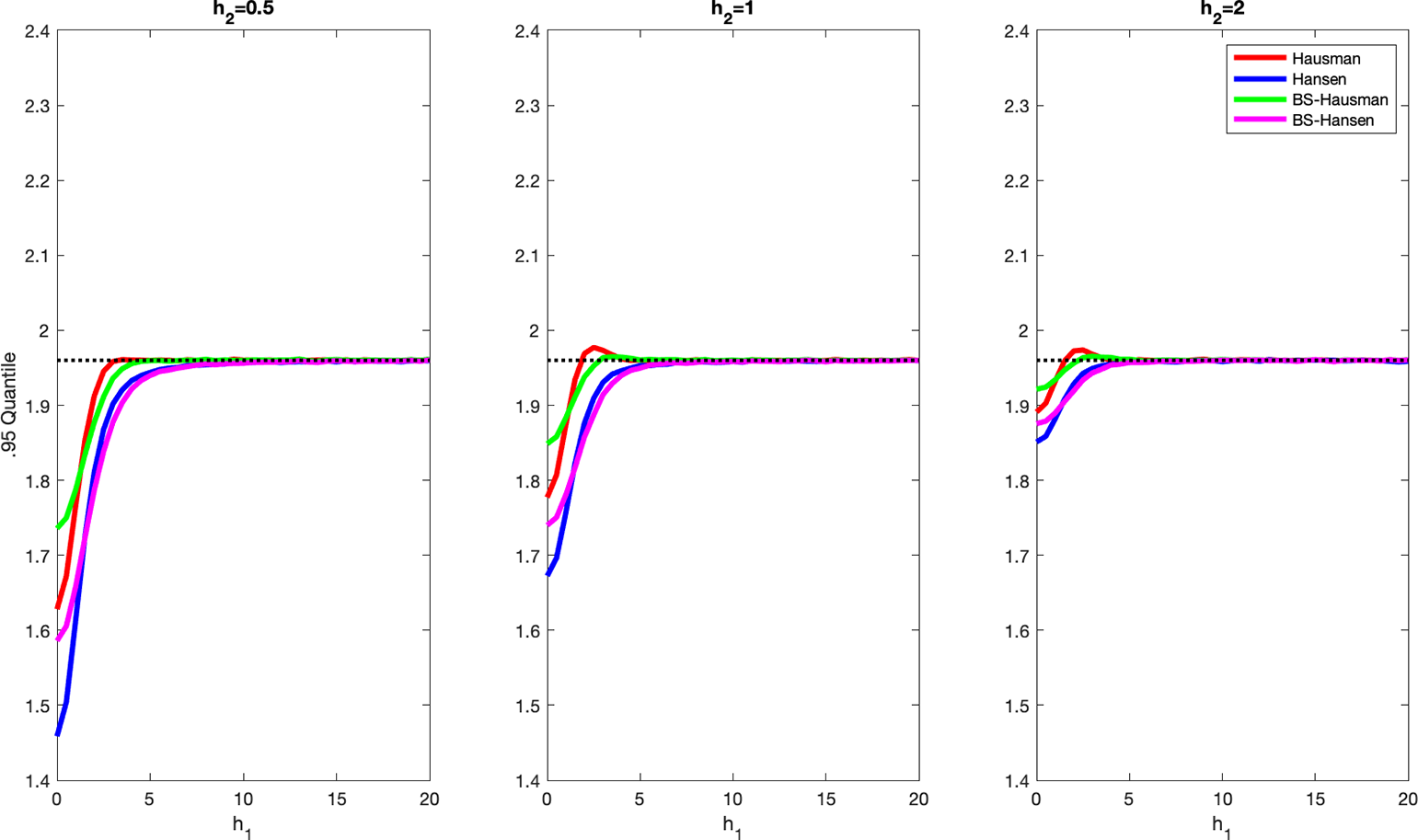
). In addition, Figure 2 shows the 95% quantiles of
 $\tilde {T}^W_{l,h}$
and
 $\tilde {T}^{W*}_{l,h}$
for
 $l \in \{\beta ,\tau \}$
as a function of
 $h_{1,ho}$
(from 0 to 20) with
 $h_{2,ho} \in \{0.5, 1, 2\}$
. We also observe smoother quantile shapes for the shrinkage statistics than for the two-stage statistics. This suggests that the shrinkage statistics may yield greater power than the Hausman-type two-stage statistics when appropriate CVs are used. Moreover, we note that similar to Figure 1, the two quantiles intersect at certain values of
 $h_{1,ho}$
, suggesting that the bootstrap tests with
 $T^W_{\beta ,n}(\theta _0)$
or
 $T^W_{\tau ,n}(\theta _0)$
do not have valid size control in general. In sum, Figures 1 and 2 suggest that the standard wild bootstrap-based two-stage or shrinkage tests are invalid in the unconditional sense, even under strong identification and conditional homoskedasticity.
95% quantiles of
 $\tilde {T}^W_{l,h}$
and
 $\tilde {T}^{W*}_{l,h}$
under strong identification and homoskedasticity.
Note: “Hausman” and “Hansen” denote the weak-identification-robust Hausman-type two-stage statistic
 $T^W_{\beta ,n}(\theta _0)$
with
 $\beta =0.05$
and Hansen’s (Reference Hansen2017) shrinkage statistic
 $T^W_{\tau ,n}(\theta _0)$
with
 $\tau =0.5$
, respectively. “BS-Hausman” and “BS-Hansen” denote their wild bootstrap analogs
 $T^{W*}_{\beta ,n}(\theta _0)$
and
 $T^{W*}_{\tau ,n}(\theta _0)$
with the dependent transformation. The results are based on 1,000,000 simulation replications.

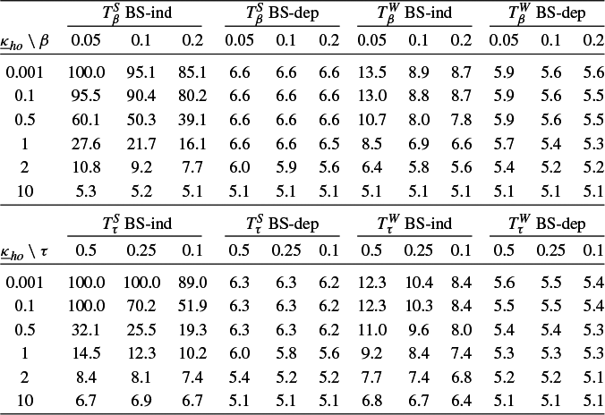
In addition, we report in Table 1 below the asymptotic null rejection probabilities of the two-stage and shrinkage tests with the independent and dependent bootstrap CVs for the homoskedastic and strong-IV case, with
 $\alpha =0.05$
for
 $\underline {\kappa }_{ho} \in \{0.001, 0.1, 0.5, 1, 2, 10\}$
, where
 $\underline {\kappa }_{ho}$
denotes the lower bound of
 $h_{2,ho}$
,
 $\beta \in \{0.05, 0.1, 0.2\}$
for the two-stage test, and
 $\tau \in \{0.1, 0.25,0 .5\}$
for the shrinkage test. First, we note that both
 $"T^S_{\beta }"$
and
 $"T^S_{\tau }"$
with independent bootstrap CVs have asymptotic rejection probabilities much larger than
 $0.05$
; e.g., when
 $\underline {\kappa }_{ho} =0.001$
, the probabilities are
 $100\%, 95.1\%, 85.1\%$
, and
 $100\%, 100\%, 89\%$
, respectively. The corresponding probabilities of
 $"T^W_{\beta }"$
and
 $"T^W_{\tau }"$
for
 $\underline {\kappa }_{ho} =0.001$
are
 $13.5\%, 8.9\%, 8.7\%$
, and
 $12.3\%, 10.4\%, 8.4\%$
, respectively. Second, we note that although the dependent bootstrap CVs yield asymptotic size distortions much smaller than those of the independent bootstrap CVs, they, in general, fail to achieve uniform size control. Third, as the heteroskedastic case nests the homoskedastic case, these results could be regarded as the lower bounds of the asymptotic size distortions under heteroskedasticity and strong identification.
Asymptotic null rejection probabilities (in %) for
 $\alpha =0.05$
under homoskedasticity

Note: “
 $T^S_{\beta }$
” and “
 $T^S_{\tau }$
” denote the Hausman-type two-stage test statistic and Hansen’s (Reference Hansen2017) shrinkage test statistic, respectively, and “
 $T^W_{\beta }$
” and “
 $T^W_{\tau }$
” denote their weak-identification-robust counterparts. “BS-ind” and “BS-dep” denote the standard wild bootstrap with independent and dependent transformation, respectively. The results are based on 1,000,000 simulation replications.
3.2 Size-Adjusted Wild Bootstrap
As illustrated in the previous section, standard wild bootstrap procedures do not provide uniform size control, even under strong identification and conditional homoskedasticity. To achieve uniform validity, including the scenarios with weak identification and heteroskedasticity, we propose, in this section, Bonferroni-based size-correction methods for the bootstrap tests based on
 $T^W_{\beta ,n}(\theta _0)$
and
 $T^W_{\tau ,n}(\theta _0)$
, the identification-robust two-stage and shrinkage statistics. As explained in McCloskey (Reference McCloskey2017), the idea behind such size-correction is to construct CVs that use the data to determine how far the key nuisance parameter (i.e., the endogeneity parameter in the current testing problem) is from the point that causes the discontinuity in the limiting distributions of the test statistics. Although the key nuisance parameter cannot be consistently estimated under the drifting sequences in (2.19), it is still possible to construct an asymptotically valid confidence set for it and then construct adaptive CVs that control the asymptotic size.
First, we will construct a size-adjusted wild bootstrap CV by using the wild bootstrap CVs with the independent transformation in Section 3.1 and Bonferroni bounds. Note that although the localization parameter
 $h_1$
cannot be consistently estimated, we may still construct an asymptotically valid confidence set for
 $h_1$
by defining
 $\hat {h}_{n,1}(\theta _0) = n^{1/2} \hat {a}(\theta _0)$
, where
 $\hat {a}(\theta _0) = \left ( \hat {v}'\hat {v} \right )^{-1}\hat {v}'\tilde {y}(\theta _0)$
. A confidence set of
 $h_1$
can be constructed by using the fact that under the drifting parameter sequences and
 $H_0: \theta = \theta _0$
,
 $$ \begin{align} \hat{h}_{n,1}(\theta_0) \rightarrow^d \tilde{h}_1\sim N \Big( h_1, h^{-2}_{25}h_{23} \Big). \end{align} $$
Then, uniformly valid size-adjusted bootstrap CVs for testing
 $H_0: \theta = \theta _0$
under
 $T^W_{\beta ,n}(\theta _0)$
or
 $T^W_{\tau ,n}(\theta _0)$
can be constructed by using Bonferroni bounds: we may construct a
 $1-(\alpha - \delta )$
level first-stage confidence set for
 $h_1$
, and then take the maximal
 $(1-\delta )$
th quantile of appropriately generated bootstrap statistics over the first-stage confidence set. Specifically, let
 $\hat {h}_{n,2} = \left (\hat {h}^{\prime }_{n,21}, vec(\hat {h}_{n,22})', \hat {h}_{n,23}, vec(\hat {h}_{n,24})',\hat {h}_{n,25} \right )'$
be the estimators of
 $h_{2}$
, and define the
 $1-(\alpha -\delta )$
level confidence set of
 $h_1$
for some
 $0<\delta \leq \alpha <1$
as
 $$ \begin{align*} CI_{_{\alpha-\delta}}(\hat{h}_{_{n,1}}(\theta_0) )& = \left[ \hat{h}_{n,1}(\theta_0) - z_{1-(\alpha-\delta)/2} \cdot \left( n \hat{V}_{a}(\theta_0) \right)^{1/2}, \; \hat{h}_{n,1}(\theta_0) \right.\\&\quad\left.+\ z_{1-(\alpha-\delta)/2} \cdot \left( n \hat{V}_{a}(\theta_0) \right)^{1/2}\right], \end{align*} $$
where
 $\hat {V}_{a}(\theta _0)$
is defined in (2.9). The wild bootstrap-based simple Bonferroni CV (SBCV) is defined as
 $$ \begin{align} c_l^{B-S} (\alpha,\alpha-\delta,\hat{h}_{n,1}(\theta_0), \hat{h}_{n,2}) = \underset{h_1 \in CI_{_{\alpha-\delta}}(\hat{h}_{n,1} (\theta_0))} \sup c^*_{l, (h_1, \hat{h}_{n,2})}(1-\delta),\; \end{align} $$
for
 $l \in \{\beta ,\tau \}$
, where
 $c^*_{l, (h_1, \hat {h}_{n,2})}(1-\delta )$
is the
 $(1-\delta )$
th quantile of the distribution of
 $T^{W*}_{l,n,(h_1, \hat {h}_{n,2})} (\theta _0)$
, i.e., the distribution of the bootstrap analog of
 $T^W_{l,n}(\theta _0)$
generated under the specific value of the localization parameter equal to
 $h_1$
.
As we saw in the previous section, standard wild bootstrap procedures do not accurately mimic the localization parameter
 $h_1$
, whether it is an independent or a dependent transformation. Therefore, for a given value of the localization parameter
 $h_1$
, we propose to generate the bootstrap two-stage test statistic
 $T^{W*}_{\beta ,n,(h_1, \hat {h}_{n,2})} (\theta _0)$
as follows:

where
 $T^*_{ols, (h_1, \hat {h}_{n,2})}(\theta _0)$
and
 $H^*_{n,(h_1, \hat {h}_{n,2})}(\theta _0)$
are the bootstrap analogs of
 $T_{ols}(\theta _0)$
and
 $H_n(\theta _0)$
, respectively, evaluated at the specific value of the localization parameter equal to
 $h_1$
. More precisely, to obtain these bootstrap analogs, we first generate the bootstrap counterparts of the OLS and regression endogeneity parameter estimators under
 $h_1$
:
 $$ \begin{align} \hat{\theta}^*_{ols, (h_1, \hat{h}_{n,2})} &= \hat{\theta}^*_{ols} +\big( \hat{h}^{\prime}_{n,21}\hat{h}_{n,24}\hat{h}_{n,21} + \hat{h}_{n,25}\big)^{-1}\hat{h}_{n,25} \left( n^{-1/2}h_1 \right), \quad \notag \\ \hat{a}^*_{(h_1, \hat{h}_{n,2})}(\theta_0) &= \hat{a}^*(\theta_0) +n^{-1/2}h_1,\; \end{align} $$
where
 $\hat {\theta }^*_{ols}$
and
 $\hat {a}^*(\theta _0)$
are generated by the standard wild bootstrap procedure in Section 3.1 with independent transformation of disturbances, so that
 $\hat {\theta }^*_{ols}$
and
 $\hat {a}^*(\theta _0)$
have localization parameter equal to zero in the bootstrap world. By doing so,
 $\sqrt {n} \left ( \hat {\theta }^*_{ols,(h_1, \hat {h}_{n,2})} - \theta _0 \right )$
and
 $\sqrt {n} \hat {a}^*_{(h_1, \hat {h}_{n,2})} (\theta _0)$
have appropriate null limiting distributions conditional on the data. Then, we obtain
 $$ \begin{align} T^*_{ols,(h_1, \hat{h}_{n,2})}(\theta_0) = (\hat{\theta}^{*}_{ols,(h_1, \hat{h}_{n,2})} - \theta_0)^2 / \hat{V}^{*}_{ols}, \quad H^*_{n,(h_1, \hat{h}_{n,2})}(\theta_0) = \hat{a}^{\ast^2}_{(h_1, \hat{h}_{n,2})}(\theta_0) / \hat{V}^{*}_{a}(\theta_0). \end{align} $$
 $T^{W*}_{\tau ,n,(h_1, \hat {h}_{n,2})} (\theta _0)$
, the bootstrap analog of the shrinkage statistic, is generated similarly.
Furthermore, we can show that the following (conditional) convergence in distribution holds:
 $$ \begin{align*} \begin{pmatrix} T^*_{ols,(h_1, \hat{h}_{n,2})}(\theta_0) \\ H^*_{n,(h_1, \hat{h}_{n,2})}(\theta_0) \end{pmatrix} \rightarrow^{d^*} \begin{pmatrix} \left(h^{\prime}_{21} h_{22}h_{21} + h_{23} \right)^{-1} \left( h^{\prime}_{21} \psi_{Ze}^{\ast} + \psi_{ve}^{\ast} + h_{25}h_1 \right)^2 \\ h_{23}^{-1} \left(\psi_{ve}^{\ast} + h_{25} h_1 \right)^{2} \end{pmatrix}, \; \notag \end{align*} $$
in probability P, where
 $\psi _{Ze}^*$
and
 $\psi _{ve}^*$
are bootstrap analogs of
 $\psi _{Ze}$
and
 $\psi _{ve}$
, respectively. This implies that conditional on the data,
 $T^{W*}_{\beta , n,(h_1, \hat {h}_{n,2})}(\theta _0)$
and
 $T^{W*}_{\tau , n,(h_1, \hat {h}_{n,2})}(\theta _0)$
, the bootstrap counterparts of the two-stage and shrinkage test statistics, have the desired null limiting distributions evaluated at the value of localization parameter equal to
 $h_1$
.
As seen in (3.4), the bootstrap SBCV equals the maximal quantile
 $c^*_{l, (h_1, \hat {h}_{n,2})} (1-\delta )$
over the values of the localization parameter
 $h_1$
in the set
 $CI_{_{\alpha -\delta }}(\hat {h}_{n,1}(\theta _0) )$
. We can now state the following asymptotic size result for
 $c_l^{B-S}(\alpha ,\alpha -\delta ,\hat {h}_{n,1}(\theta _0), \hat {h}_{n,2})$
, where
 $l \in \{\beta ,\tau \}$
.
Theorem 3.1. Suppose that
 $H_0$
holds, then we have for any
 $\;0<\delta \leq \alpha <1$
and for
 $l \in \{\beta , \tau \}$
,
 $AsySz \left [c_l^{B-S} (\alpha ,\alpha -\delta ,\hat {h}_{n,1}(\theta _0), \hat {h}_{n,2})\right ] \leq \alpha .$
Theorem 3.1 states that tests based on
 $c_l^{B-S} (\alpha ,\alpha -\delta ,\hat {h}_{n,1}(\theta _0),\hat {h}_{n,2})$
control the asymptotic size. In practice,
 $c_l^{B-S} (\alpha ,\alpha -\delta ,\hat {h}_{n,1}(\theta _0),\hat {h}_{n,2})$
can be obtained by using the following algorithm.
Wild Bootstrap Algorithm for
 $\boldsymbol {c_l^{B-S} (\alpha ,\alpha -\delta ,\hat {h}_{_{n,1}}(\theta _0),\hat {h}_{_{n,2}})}$
:
-
1. Generate the bootstrap statistics
$\left \{\hat {\theta }^{*(b)}_{ols}, \hat {a}^{*(b)}(\theta _0), \hat {V}^{*(b)}_{ols}, \hat {V}^{*(b)}_{a}(\theta _0), T^{*(b)}_{ar}(\theta _0) \right \}, b=1, \ldots , B,$
using the standard wild bootstrap procedure with independent transformation of disturbances. -
2. Choose
$\alpha $
,
$\delta $
, and compute
$CI_{_{\alpha -\delta }}(\hat {h}_{n,1} (\theta _0))$
. Create a fine grid for
$CI_{_{\alpha -\delta }}(\hat {h}_{n,1} (\theta _0))$
and call it
$\mathscr {C}^{grid}_{_{\alpha -\delta }}.$
-
3. For
$l \in \{\beta , \tau \}$
and for
$h_1 \in \mathscr {C}^{grid}_{_{\alpha -\delta }}$
, generate
$T^{W*(b)}_{l, n, (h_1, \hat {h}_{n,2})}(\theta _0)$
,
$b=1, \ldots , B$
, using the bootstrap statistics generated in Step 1. The same set of bootstrap statistics can be used repeatedly for each
$h_1$
. -
4. Compute
$c^*_{l, (h_1, \hat {h}_{n,2})}(1-\delta )$
, the
$(1-\delta )$
th quantile of the distribution of
$T^{W*}_{l, n, (h_1, \hat {h}_2)}(\theta _0)$
from these B draws of bootstrap samples. -
5. Find
$c_l^{B-S} (\alpha ,\alpha -\delta ,\hat {h}_{_{n,1}}(\theta _0), \hat {h}_{n,2}) = \underset { h_1 \in \mathscr {C}^{grid}_{_{\alpha -\delta }}}\sup c^*_{l, (h_1, \hat {h}_{n,2})}(1-\delta ).$
-
6. Reject
$H_0: \theta = \theta _0$
if
$T^W_{l,n}(\theta _0)> c_l^{B-S} (\alpha ,\alpha -\delta ,\hat {h}_{_{n,1}}(\theta _0), \hat {h}_{n,2})$
.


Note that, as shown in Theorem 3.1, although controlling the asymptotic size, the bootstrap SBCV defined above may yield a conservative test whose asymptotic size does not reach its nominal level. For further refinement on the Bonferroni bounds, we propose a size-adjustment method to adjust the bootstrap SBCV so that the resulting test is not conservative with an asymptotic size exactly equal to
 $\alpha $
. Specifically, for
 $l \in \{\beta , \tau \}$
, the size-adjustment factor for the bootstrap SBCV is defined as
 $$ \begin{align} \hat{\eta}_{l,n} = \inf \left\{\! \eta: \underset{h_1 \in \mathscr{H}_1} \sup P^* \left[\! T^{W*}_{l, n, (h_1, \hat{h}_{n,2})} (\theta_0)\!>\! c_l^{B-S} (\alpha, \alpha-\delta, \hat{h}^*_{n,1} (\theta_0, h_1), \hat{h}_{n,2}) + \eta \!\right] \!\leq \alpha \!\right\}, \end{align} $$
where
 $\hat {h}^*_{n,1}(\theta _0, h_1)$
denotes the bootstrap analog of
 $\hat {h}_{n,1}(\theta _0)$
with localization parameter equal to
 $h_1$
and is generated by the same bootstrap samples as those of
 $T^{W*}_{n, (h_1, \hat {h}_{n,2})} (\theta _0)$
. More precisely, we define
 $$ \begin{align} \hat{h}^*_{n,1} (\theta_0, h_1) = \hat{h}^*_{n,1}(\theta_0) + h_1, \end{align} $$
where
 $\hat {h}^*_{n,1}(\theta _0) = n^{1/2} \hat {a}^{\ast }(\theta _0) = \big (\hat {v}^{*\prime } \hat {v}^*\big )^{-1} \hat {v}^{*\prime }u^*$
,
 $\hat {v}^*=M_{Z}X^*,$
is generated by the standard wild bootstrap procedure with independent transformation so that the localization parameter equals zero in the bootstrap world. Notice that we have the following convergence in distribution (jointly with the other bootstrap statistics):
 $ \hat {h}^*_{n,1} (\theta _0, h_1) \rightarrow ^{d^*} N \Big ( h_1, h^{-2}_{25}h_{23} \Big ), $
in probability P, i.e., the same limiting distribution as that of
 $\hat {h}_{n,1}(\theta _0)$
in (3.3), under the specific value of
 $h_1$
.
The goal of the size-adjustment method is to decrease the bootstrap SBCV as much as possible by using the factor
 $\eta $
while not violating the inequality in (3.8), so that the asymptotic size of the resulting tests can be controlled. Then, the bootstrap size-adjusted CV (BACV) can be defined as
 $$ \begin{align} & c_l^{B-A} (\alpha,\alpha-\delta,\hat{h}_{n,1}(\theta_0), \hat{h}_{n,2}) \notag \\ &\quad= c_l^{B-S} (\alpha,\alpha-\delta,\hat{h}_{n,1}(\theta_0), \hat{h}_{n,2}) + \hat{\eta}_{l,n} \;\; \text{for} \;\; l \in \{\beta, \tau\}, \end{align} $$
and one can expect that relatively small
 $\hat {\eta }_{l,n}$
results in a relatively less conservative (and more powerful) test. Furthermore, we notice that the bootstrap-based size-adjustment method in (3.10), which employs a size-adjustment factor, is in the same spirit as the adjusted Bonferroni CV proposed in McCloskey (Reference McCloskey2017, Sect. 3.2), which is based on adjusting the quantile level of the underlying localized quantile in the SBCV.
Below, we state the theorem on the uniform size control of wild bootstrap CVs using the size-adjustment method. We assume a continuity condition on the NRP function, following similar continuity assumptions in Andrews and Cheng (Reference Andrews and Cheng2012, p. 2195, Assump. Rob2(i)) and Han and McCloskey (Reference Han and McCloskey2019, p. 1052, Assump. DF2(ii)). Define
 $c^{B-S}_l(\alpha , \alpha -\delta , \tilde {h}_1, h_2) = \sup _{h_1 \in CI_{\alpha -\delta } (\tilde {h}_1)} c_{l,h} (1-\delta )$
, where
 $c_{l,h}(1-\delta )$
is the
 $(1-\delta )$
th quantile of
 $\tilde {T}^W_{l,h}$
, and
 $\tilde {T}^W_{l,h}$
is the weak limit of
 $T^W_{l,n}(\theta _0)$
under the sequence
 $\{\gamma _{n,h}\} \subset \Gamma $
satisfying (2.19) for
 $l \in \{\beta , \tau \}$
.
Assumption 1.
 $P\left [\tilde {T}^W_{l,h} = c_l^{B-S}(\alpha , \alpha -\delta , \tilde {h}_1, h_2) + \eta \right ]=0$
,
 $\forall h_1 \in \mathscr {H}_1$
and
 $\eta \in [-c_l^{B-S}(\alpha , \alpha -\delta , \tilde {h}_1, h_2), 0]$
, where
 $l \in \{\beta , \tau \}$
.
Theorem 3.2. Suppose that
 $H_0$
and Assumption 1 hold, then we have for any
 $\;0<\delta \leq \alpha <1$
, and for
 $l \in \{\beta , \tau \}$
:
 $AsySz \big [c_l^{B-A} (\alpha ,\alpha -\delta , \hat {h}_{n,1}(\theta _0), \hat {h}_{n,2})\big ] = \alpha .$
Furthermore, let
 $CS_{l,n}(1-\alpha )$
denote the confidence set of the nominal level
 $1-\alpha $
for
 $\theta $
constructed by collecting all values of
 $\theta $
that cannot be rejected by the corresponding two-stage or shrinkage size-adjusted test at the nominal level
 $\alpha $
.
Corollary 3.1. Suppose that Assumption 1 holds, then we have for any
 $\;0<\delta \leq \alpha <1$
and for
 $l \in \{\beta , \tau \}$
:
 $\liminf _{n\,\rightarrow \,\infty }\inf _{\gamma \;\in \;\Gamma }P_{_{\theta , \gamma }} \left [ \theta \in CS_{l,n}(1-\alpha ) \right ] = 1-\alpha .$
Theorem 3.2 shows that
 $c_l^{B-A} (\alpha ,\alpha -\delta ,\hat {h}_{n,1}(\theta _0), \hat {h}_{n,2})$
yield two-stage and shrinkage bootstrap tests with the correct asymptotic size, irrespective of identification strength, and Corollary 3.1 states that the confidence sets constructed from inverting these tests have correct asymptotic coverage probability.Footnote
18
To implement such size-adjusted tests in practice, we must compute
 $c_l^{B-S} (\alpha ,\alpha -\delta ,\hat {h}_{_{n,1}}(\theta _0),\hat {h}_{n,2})$
and
 $\hat {\eta }_{l,n}$
. These values can be computed sequentially starting with
 $c_{l}^{B-S} (\alpha ,\alpha -\delta ,\hat {h}_{n,1}(\theta _0),\hat {h}_{n,2})$
. Then the size-adjustment factor
 $\hat {\eta }_{l,n}$
can be calculated by evaluating (3.8) on a fine grid of
 $\mathscr {H}_1$
as follows.
Wild Bootstrap Algorithm for
 $\boldsymbol {c_l^{B-A} (\alpha ,\alpha -\delta ,\hat {h}_{_{n,1}}(\theta _0),\hat {h}_{_{n,2}})}$
:
-
1. Generate bootstrap statistics
$\left \{\hat {\theta }^{*(b)}_{ols}, \hat {a}^{*(b)}(\theta _0), \hat {V}^{*(b)}_{ols}, \hat {V}^{*(b)}_{a}(\theta _0), T^{*(b)}_{ar}(\theta _0) \right \}, b=1, \ldots , B,$
using the standard wild bootstrap procedure with independent transformation. -
2. For
$l \in \{\beta , \tau \}$
, let
$c_l^{B-S} (\alpha ,\alpha -\delta ,\hat {h}_{n,1} (\theta _0),\hat {h}_{n,2})$
be the obtained SBCV. -
3. Create a fine grid of the set
$\mathscr {H}_1$
in (3.8) and call it
$\mathscr {H}^{grid}_1$
. For
$l \in \{\beta , \tau \}$
and for each
$h_1 \in \mathscr {H}^{grid}_1$
, obtain
$T^{W*(b)}_{l, n,(h_1, \hat {h}_{n,2})} (\theta _0)$
and
$c_l^{B-S} (\alpha , \alpha -\delta , \hat {h}^{*(b)}_{n,1} (\theta _0, h_1), \hat {h}_{n,2})$
,
$b=1, \ldots , B$
, using the bootstrap statistics generated in Step 1. Note that the same set of bootstrap statistics can be used for each
$h_1$
. -
4. Create a fine grid of
$[-c_l^{B-S} (\alpha ,\alpha -\delta ,\hat {h}_{n,1}(\theta _0), \hat {h}_{n,2}),\,0]$
and call it . -
5. Find all
s.t. and set
$\hat {\eta }_{l,n}$
equal to the smallest
$\eta $
.
-
6. The BACV is given by
$c_l^{B-A} (\alpha ,\alpha -\delta ,\hat {h}_{n,1}(\theta _0), \hat {h}_{n,2}) = c_l^{B-S} (\alpha ,\alpha -\delta ,\hat {h}_{n,1}(\theta _0), \hat {h}_{n,2}) + \hat {\eta }_{l,n}.$
-
7. Reject
$H_0: \theta = \theta _0$
if
$T^W_{l,n}(\theta _0)> c_l^{B-A} (\alpha ,\alpha -\delta ,\hat {h}_{_{n,1}}(\theta _0), \hat {h}_{n,2})$
.


 .
 s.t.


Several remarks are in order. First, we emphasize that
 $\hat {h}^*_{n,1}(\theta _0, h_1)$
needs to be generated simultaneously with
 $T^{W*}_{l, n, (h_1, \hat {h}_{n,2})} (\theta _0)$
using the same bootstrap samples, so that the dependence structure between the statistics
 $T^W_{l, n}(\theta _0)$
and
 $\hat {h}_{n,1}(\theta _0)$
is well mimicked by the bootstrap statistics. This is important for the size-adjustment procedure to correct the conservativeness of the Bonferroni bound. Similarly, for the implementation of the size adjustment, one cannot replace
 $c_l^{B-S} (\alpha , \alpha -\delta , \hat {h}^*_{n,1} (\theta _0, h_1), \hat {h}_{n,2}) $
in (3.8) with
 $c_l^{B-S} (\alpha , \alpha -\delta , \hat {h}_{n,1}(\theta _0), \hat {h}_{n,2})$
, as it also breaks down the dependence structure.
Second, when
 $|h_1| = \infty $
,
 $H_n(\theta _0)$
diverges to infinity, so that
 $T^W_{\beta ,n}(\theta _0)$
and
 $T^W_{\tau ,n}(\theta _0)$
are equal to
 $T_{ar}(\theta _0)$
with probability approaching 1. Furthermore, when
 $|h_1| = \infty $
,
 $\hat {h}_{n,1}(\theta _0)$
and thus the confidence interval
 $CI_{\alpha - \delta }(\hat {h}_{n,1}(\theta _0))$
also diverge to infinity. We note that the bootstrap SBCV is equal to
 $\sup _{ h_1 \in CI_{\alpha - \delta } (\hat {h}_{n,1}(\theta _0))} c^*_{l, (h_1, \hat {h}_{n,2})} (1-\delta ), $
where
 $l \in \{\beta , \tau \}$
, and
 $c^*_{l, (h_1, \hat {h}_{n,2})} (1-\delta )$
denotes the
 $(1-\delta )$
th quantile of the bootstrap version of the two-stage/shrinkage statistic under the specific value of
 $h_1$
. Therefore, when
 $|h_1| = \infty $
, the SBCV will be equal to the corresponding quantile of
 $T^*_{ar}(\theta _0)$
(i.e., the bootstrap version of
 $T_{ar}(\theta _0)$
) with probability approach 1. As a result, the limiting NRP of our proposed bootstrap tests is controlled in this case as well. In addition, our size-adjustment factor
 $\hat {\eta }_{l,n}$
in the BACV will decrease the SBCV as much as possible to achieve the correct asymptotic size.
Third, we note that in finite samples, as the transition between the OLS and IV-based methods can be relatively abrupt for the two-stage statistic compared to the shrinkage statistic, the finite sample behavior of the size-adjusted bootstrap tests with
 $T^W_{\beta ,n}(\theta _0)$
may be closer to that of
 $T_{ar}(\theta _0)$
(this is also observed in our simulations).
3.3 Extension to Clustered Data
Many applications in economics involve error terms that are correlated within clusters (see, e.g., Cameron and Miller, Reference Cameron and Miller2015 and the references therein), and various studies in the literature on cluster-robust inference recommend using wild cluster bootstrap as a way to obtain more accurate inference, including Cameron et al. (Reference Cameron, Gelbach and Miller2008), MacKinnon and Webb (Reference MacKinnon and Webb2017), Djogbenou et al. (Reference Djogbenou, MacKinnon and Nielsen2019), and MacKinnon et al. (Reference MacKinnon, Nielsen and Webb2023), among others. However, by using arguments similar to those for the IV model with heteroskedastic errors, we can show that the standard wild cluster bootstrap is invalid in the current context for the two-stage testing and shrinkage procedures. In this section, we extend the (weak-identification-robust) size-adjusted bootstrap procedure proposed in Section 3.2 to the case with clustered samples.
To proceed, consider the following linear IV model with clustered data:
 $$ \begin{align} y_g = X_g \theta + u_g, \quad X_g = Z_g \pi + v_g, \end{align} $$
where
 $y_g = (y_{g1}, \ldots , y_{g n_g})'$
,
 $X_g=(X_{g1}, \ldots , X_{gn_g})'$
, and
 $Z_g=(Z_{g1}, \ldots , Z_{gn_g})'$
denote an
 $n_g \times 1$
vector of dependent variables, an
 $n_g \times 1$
vector of endogenous regressors, and an
 $n_g \times k$
matrix of instruments for the gth cluster, respectively. Let G denote the number of clusters and n denote the total number of observations. Similar to the case with heteroskedastic data, we can define the extended regression
 $$ \begin{align} y_g = X_g \theta + v_g a^c + e_g, \end{align} $$
where
 $a^c = \left (n^{-1} \sum _{g=1}^G E_F[v_g'v_g] \right )^{-1} \left (n^{-1} \sum _{g=1}^G E_F[v_g' u_g] \right )$
, and the weak identification and cluster-robust test statistic for the null of exogeneity
 $H^c_a: a^c=0$
takes the form of
 $$ \begin{align} H^c_n(\theta_0) = (\hat{a}^{c}(\theta_0))^2/ \hat{V}^c_a(\theta_0), \end{align} $$
where
 $\hat {V}^c_a(\theta _0) = (n^{-1} \hat {v}'\hat {v})^{-1} \left ( n^{-2} \sum _{g=1}^G \hat {v}_g' \hat {e}_g (\theta _0) \hat {e}(\theta _0)' \hat {v}_g \right ) (n^{-1} \hat {v}' \hat {v})^{-1}, \hat {a}^c(\theta _0) = (\hat {v}'\hat {v})^{-1} \hat {v}'\tilde {y}(\theta _0)$
,
 $\hat {v}'\hat {v} = \sum _{g=1}^G \hat {v}_g' \hat {v}_g$
, and
 $\hat {v}'\tilde {y}(\theta _0) = \sum _{g=1}^G \hat {v}_g'\tilde {y}_g(\theta _0)$
. In the same fashion, we define
 $T^c_{ols}(\theta _0)$
and
 $T^c_{ar}(\theta _0)$
, the cluster-robust OLS-based Wald and AR statistics, following the definitions in the heteroskedastic case. Then, the weak identification and cluster-robust two-stage test statistic
 $T^{Wc}_{\beta ,n}(\theta _0)$
and shrinkage test statistic
 $T^{Wc}_{\tau ,n}(\theta _0)$
can be defined according to the definitions in Section 2.1, i.e.,

For clustered data, we define the vector of nuisance parameters
 $\gamma _n^c = (\gamma ^c_{n,1}, \gamma ^c_{n,2}, \gamma ^c_{n,3})$
by
 $$ \begin{align} \gamma^c_{n,1} = a_n^c, \;\; \gamma^c_{n,2} = (\gamma^c_{n,21},\gamma^c_{n,22},\gamma^c_{n,23},\gamma^c_{n,24},\gamma^c_{n,25}),\;\; \gamma^c_{n,3} = F_n, \end{align} $$
and the corresponding parameter space by
 $\Gamma ^c = \{ \gamma ^c_n = (\gamma ^c_{n,1}, \gamma ^c_{n,2}, \gamma ^c_{n,3}): \gamma ^c_{n,1} \in \Gamma ^c_1, \gamma ^c_{n,2} \in \Gamma ^c_2, \gamma ^c_{n,3} \in \Gamma ^c_3(\gamma ^c_{n,1}, \gamma ^c_{n,2}) \}$
, where
 $$ \begin{align} & \Gamma^c_1= \mathbb{R}, \;\; \Gamma^c_2 = \Big\{(\gamma^c_{n,21},\gamma^c_{n,22},\gamma^c_{n,23},\gamma^c_{n,24},\gamma^c_{n,25}): \gamma^c_{n,21} = \pi_n \in \mathbb{R}^k, \notag \\ & \gamma^c_{n,22} = \mu_{n} \left( n^{-2} \sum_{g=1}^G E_{F_n} Z_g' e_g e_g' Z_g \right) \in \mathbb{R}^{k \times k}, \Big. \notag \\ & \gamma^c_{n,23}= \mu_n \left( n^{-2} \sum_{g=1}^G E_{F_n} v_g' e_g e_g' v_g \right) \in \mathbb{R}, \notag \\ & \gamma^c_{n,24}= n^{-1} \sum_{g=1}^G E_{F_n} Z_g' Z_g \in \mathbb{R}^{k \times k}, \gamma^c_{n,25}= n^{-1} \sum_{g=1}^G E_{F_n} v_g'v_g \in \mathbb{R}, \Big. \notag \\ & \textit{s.t.}\;\; \lambda_{min}(\gamma^c_{n,22}) \geq \underline{\kappa}, \gamma^c_{n,23}> 0, \lambda_{min}(\gamma^c_{n,24}) \geq \underline{\kappa}, \; \text{and} \; \gamma^c_{n,25} > 0 \Big\}, \end{align} $$
for some
 $\underline {\kappa }>0 $
that does not depend on n, and
 $\{ \mu _n \}$
is a non-random sequence, which plays a similar role as that used in Djogbenou et al. (Reference Djogbenou, MacKinnon and Nielsen2019) and is needed because different from the model with heteroskedastic errors, the convergence rate of the estimators
 $\hat {\theta }^c_{ols}$
and
 $\hat {a}^c(\theta _0)$
under clustering depends on various factors, such as the regressor, the relative cluster size, and the intra-cluster correlation (also see Hansen and Lee, Reference Hansen and Lee2019, Sect. 4 for related discussions). As pointed out by Djogbenou et al. (Reference Djogbenou, MacKinnon and Nielsen2019), the sequence
 $\{ \mu _n \}$
can be interpreted as the rate at which information accumulates, and because of the studentization of the test statistics,
 $\{ \mu _n \}$
needs not be known in practice, but only needs to exist. Furthermore, we allow for the case with weak identification under clustering.
In addition,
 $\Gamma ^c_3(\gamma ^c_{n,1}, \gamma ^c_{n,2})$
is defined as follows:
 $$ \begin{align} & \Gamma^c_3(\gamma^c_{n,1}, \gamma^c_{n,2}) = \Big\{ F_n: \; E_{F_n} e_g' v_g = E_{F_n} Z_g'e_g = E_{F_n} Z_g'v_g = 0,\; \notag \\ & E_{F_n} Z_g'e_g e_g'v_g = E_{F_n} Z_g' v_g e_g'v_g = E_{F_n} Z_g' e_g v_g' Z_g =0,\; \Big. \notag \\ & \mu_n \left( n^{-2} \sum_{g=1}^G E_{F_n} Z_g'v_g v_g'Z_g \right) \in \mathbb{R}^{k \times k} \;\; \text{with} \;\; \lambda_{min} \left( \mu_n n^{-2} \sum_{g=1}^G E_{F_n} Z_g'v_g v_g'Z_g \right) \geq \underline{\kappa}, \; \Big. \notag \\ & \left\lVert \sup_{g,i} E_{F_n} \left( ||Z_{gi} e_{gi}||^{2+\xi}, ||Z_{gi} v_{gi}||^{2+\xi}, |v_{gi}e_{gi}|^{2+\xi}, || Z_{gi} Z_{gi}' ||^{2+\xi}, |X_{gi}|^{2(2+\xi)} \right)'\right\rVert \leq M \Big\}, \notag \\ \end{align} $$
for some constant
 $\underline {\kappa }>0, \xi >0$
,
 $M<\infty $
, and
 $\{ \mu _n \}$
is the non-random sequence defined above. We then define the whole nuisance parameter space
 $\Gamma ^c$
of
 $\gamma ^c_n$
as
 $ \Gamma ^c = \{ \gamma ^c_n = (\gamma ^c_{n,1}, \gamma ^c_{n,2}, \gamma ^c_{n,3}): \gamma ^c_{n,1} \in \Gamma ^c_1, \gamma ^c_{n,2} \in \Gamma ^c_2, \gamma ^c_{n,3} \in \Gamma ^c_3(\gamma ^c_{n,1}, \gamma ^c_{n,2})\}. $
Now, let us define
 $$ \begin{align} \mathscr{H}^c &= \Bigg\{ h^c = (h^c_1, h^{c'}_{21},vec(h^c_{22})', h^c_{23},vec(h^c_{24})', h^c_{25})' \in \mathbb{R}^{2k^2+k+3}_{\infty}: \notag \\ & \quad \exists \{\gamma^c_n = (\gamma^c_{n,1}, \gamma^c_{n,2}, \gamma^c_{n,3}) \in \Gamma^c: n \geq 1\} \quad s.t. \Big.\notag\\ &\quad \mu_n^{1/2}\gamma^c_{n,1} \rightarrow h^c_1 \in \mathbb{R}_{\infty},\;\;\gamma^c_{n,2} \rightarrow h^c_2=(h^c_{21},h^c_{22}, h^c_{23},h^c_{24},h^c_{25}), \; \lambda_{min}(A)\geq \underline{\kappa} \Big.\notag\\ & \;\;\;\; \text{for}\;\;A\in \{ h^c_{22}, h^c_{24}\}, \; h^c_{23}>0, \; h^c_{25}>0 \Bigg\} \; \end{align} $$
for some
 $\underline {\kappa }>0$
and
 $\mathbb {R}_{\infty } = \mathbb {R} \cup \{ \pm \infty \}.$
Similar to the heteroskedastic case, to derive the asymptotic size, it suffices to study the asymptotic NRP along a certain sequence
 $\{\gamma ^c_{n,h}\}$
for some
 $h^c \in \mathscr {H}^c$
, with
 $\gamma ^c_{n,h} = ( \gamma ^c_{n,h,1}, \gamma ^c_{n,h,2}, \gamma ^c_{n,h,3} )$
satisfying:
 $$ \begin{align} \mu_n^{1/2}\gamma^c_{n,h,1} \rightarrow h^c_1, \; \gamma^c_{n,h,2} \rightarrow h^c_2, \; \text{and} \; \gamma^c_{n,h,3} = F_n \in \Gamma^c_3(\gamma^c_{n,h,1}, \gamma^c_{n,h,2}). \end{align} $$
Now, we present the algorithm for the wild cluster bootstrap procedure with the independent transformation, which will be used to construct uniformly valid bootstrap CVs under clustering.
Wild Cluster Bootstrap Algorithm:
-
1. Given
$H_0: \theta = \theta _0$
, compute the residuals from the first-stage and structural equations:
$\hat {v}_g = X_g -Z_g \hat {\pi }, \hat {u}_g(\theta _0) = y_g - X_g \theta _0$
, where
$\hat {\pi }=(Z^{\prime }Z)^{-1}Z^{\prime }X=\left (\sum _{g=1}^G Z_g'Z_g \right )^{-1} \sum _{g=1}^G Z_g'X_g$
. -
2. Generate the cluster-level bootstrap pseudo-data following
$X^{\ast }_g = Z_g \hat {\pi } + v^{\ast }_g, y^{\ast }_g = X_g^{\ast }\theta _0 + u^{\ast }_g$
, where
$v^*_g = \hat {v}_g \omega ^*_{1g}$
, and
$u^*_g = \hat {u}_g(\theta _0) \omega ^*_{2g}$
, for each
$g=1, \ldots , G$
, where
$\omega ^*_{1g}$
and
$\omega ^*_{2g}$
are two random variables that have mean zero and variance
$1$
, are independent from the data and independent from each other. -
3. Compute
$\left \{\hat {\theta }^{c*}_{ols}(\theta _0), \hat {a}^{c*}(\theta _0), \hat {V}^{c*}_{ols}, \hat {V}^{c*}_{a}(\theta _0), T^{c*}_{ar}(\theta _0) \right \}$
by the bootstrap samples generated in Step 2.


Then, for a given value of
 $\dot {h}_1^c$
, we generate the bootstrap test statistics as follows:
 $$ \begin{align} & T^{c*}_{ols,(\dot{h}^c_1, \hat{h}^c_{n,2})}(\theta_0) \notag \\ &= \left( \left( \hat{\theta}^{c*}_{ols} - \theta_0 \right) / \hat{V}^{c*1/2}_{ols} + \left(\hat{h}_{n,21}^{c'} \hat{h}_{n,24}^c \hat{h}_{n,21}^c + \hat{h}_{n,25}^c\right)^{-1} \hat{h}_{n,25}^c \left(\hat{V}_a^{c*}(\theta_0) /\hat{V}_{ols}^{c*}\right)^{1/2} \dot{h}_1^c\right)^2, \quad \notag \\ & \text{and} \;\; H^{c*}_{n,(\dot{h}^c_1, \hat{h}^c_{n,2})} (\theta_0) = \left( \hat{a}^{c*}(\theta_0) / \hat{V}^{c*1/2}_a(\theta_0) + \dot{h}_{1}^c \right)^2, \end{align} $$
where
 $\hat {h}_{n,21}^c = \left (\sum _{g=1}^G Z_g'Z_g \right )^{-1} \sum _{g=1}^G Z_g'X_g$
,
 $\hat {h}_{n,24}^c = n^{-1} \sum _{g=1}^G Z_g'Z_g$
, and
 $\hat {h}_{n,25}^c = n^{-1} \sum _{g=1}^G \hat {v}_g'\hat {v}_g$
.
The bootstrap analogs of the two-stage and shrinkage test statistics evaluated at
 $\dot {h}_1^c$
,
 $T^{Wc*}_{l, n,(\dot {h}^c_1, \hat {h}^c_{n,2})} (\theta _0)$
, can be obtained subsequently. Notice that because of the appropriate studentization,
 $\{ \mu _n \}$
is also not needed in the procedure described by (3.20).
Now, let
 $CI_{_{\alpha -\delta }}(\hat {\dot {h}}^c_{n,1})$
denote the
 $1-(\alpha -\delta )$
level confidence set for
 $\dot {h}^c_1$
for some
 $0<\delta \leq \alpha <1$
, where
 $\hat {\dot {h}}^c_{n,1} = \hat {a}^c(\theta _0) / (\hat {V}^{c}_a(\theta _0))^{1/2}$
. The SBCV for clustered data is then defined as
 $$ \begin{align} c_l^{B-S} (\alpha,\alpha-\delta,\hat{\dot{h}}^c_{n,1}, \hat{h}^c_{n,2}) = \underset{\dot{h}^c_1 \in CI_{_{\alpha-\delta}}(\hat{\dot{h}}^c_{n,1})} \sup c^*_{l, (\dot{h}^c_1, \hat{h}^c_{n,2})}(1-\delta) \; \text{for} \; l \in \{\beta,\tau\}, \end{align} $$
where
 $c^*_{l, (\dot {h}^c_1, \hat {h}^c_{n,2})}(1-\delta )$
is the
 $(1-\delta )$
th quantile of the distribution of
 $T^{Wc*}_{l, n,(\dot {h}^c_1, \hat {h}^c_{n,2})} (\theta _0)$
, which is the bootstrap analog of
 $T^{Wc}_{l,n}(\theta _0)$
generated under the value of the localization parameter equal to
 $\dot {h}^c_1$
. The specific size-adjusted bootstrap algorithm for the SBCV closely follows that for heteroskedastic data in Section 3.2 and is thus omitted for conciseness.
For further refinement on the Bonferroni bound, we define the size-adjustment factor
 $\hat {\eta }^c_{l,n}$
following (3.8). Then, the BACV for the case with clustered data can be defined as
 $$ \begin{align} c_l^{B-A} (\alpha,\alpha-\delta,\hat{\dot{h}}^c_{n,1}(\theta_0), \hat{h}^c_{n,2}) = c_l^{B-S} (\alpha,\alpha-\delta,\hat{\dot{h}}^c_{n,1}(\theta_0), \hat{h}^c_{n,2}) + \hat{\eta}^c_{l,n}. \end{align} $$
Similarly, its algorithm follows closely that described in Section 3.2.
For the sake of conciseness, we present the asymptotic validity results for our size-adjusted bootstrap tests under clustering in Section S.4 of the Supplementary Material.
4 FINITE SAMPLE POWER PERFORMANCE
In this section, we study the finite-sample power performance of the size-adjusted wild bootstrap procedure by conducting simulations for the linear IV model under conditional heteroskedasticity or clustering. For all simulations, the number of Monte Carlo replications is set at
 $5,000$
, and the number of bootstrap replications is set at
 $B=399$
. We compare the performance of the (heteroskedasticity or cluster-robust) AR test with the asymptotic CVs (without pretest or shrinkage), the two-stage test based on the size-adjusted wild bootstrap CVs, and the test based on Hansen’s (Reference Hansen2017) shrinkage approach and its corresponding size-adjusted wild bootstrap CVs. We set
 $\alpha =0.05$
for the CVs of the three tests. Here, we use the AR test instead of the IV-based t-test as the IV-based t-test cannot control size under weak identification and high levels of endogeneity (e.g., it will have size distortions when
 $| \rho |> 0.565$
in the case with one IV, according to Angrist and Kolesár, Reference Angrist and Kolesár2024). In addition, we set
 $\beta =0.05$
as the nominal level of the pretest. In Section S.5 of the Supplementary Material, we provide further Monte Carlo simulation results with other choices of
 $\beta $
and
 $\delta $
, with negative values of the endogeneity parameter, and for the overidentified case. All of them show patterns similar to those reported here. The shrinkage parameter
 $\tau $
in Hansen’s (Reference Hansen2017) procedure is set to equal 0.5 or 0.25. The random weights for the wild bootstrap are generated from the standard normal distribution throughout the simulations.
First, we study the case with heteroskedastic errors. The simulation model follows the IV model in (2.1), and the DGP is specified as
 $$ \begin{align} & (\tilde{u}_{i}, \tilde{\epsilon}_{i})' \sim i.i.d. \; N(0, I_2), \; Z_i \sim i.i.d. \; N(0,1), \; \text{and is independent from} \; (\tilde{u}_{i}, \tilde{\epsilon}_{i})', \notag \\ & \tilde{v}_{i} = \rho \tilde{u}_{i} + (1-\rho^2)^{1/2} \tilde{\epsilon}_{i}, \; u_{i} = f(Z_{i}) \tilde{u}_{i}, \; \text{and} \; v_{i} = f(Z_{i}) \tilde{v}_{i}, \end{align} $$
where
 $i=1, \ldots , n$
and
 $f(x)=|x|$
. The sample size is set at
 $n=200$
for the heteroskedastic case. The value of the null hypothesis
 $\theta _0$
is fixed at zero throughout the simulations. Following the IV literature, we capture instrument strength by using the concentration parameter
 $\phi = \pi ^2 \cdot Z'Z$
and set
 $\phi \in \{1, 10\}$
. We allow the IV to be very weak as all the tests considered in the simulations are weak-IV-robust. In addition, the true values of the endogeneity parameter
 $\rho $
are set at
 $\rho \in \{0.1, 0.5, 0.99\}$
. Here, we focus on the case with one IV as it is the leading case in empirical applications (e.g., 101 of 230 specifications in the sample of Andrews et al., Reference Andrews, Stock and Sun2019, 1,087 of 1,359 in the sample of Young, Reference Young2022, and 1,311 in the sample of Lee et al., Reference Lee, McCrary, Moreira and Porter2022). We further report simulation results for the overidentified case in the Supplementary Material.
Figures 3 and 4 show the finite-sample power curves of the tests under heteroskedasticity with
 $\phi = 1$
and
 $10$
, respectively.
 $\beta $
and
 $\delta $
are set equal to
 $0.05$
and
 $0.025$
, respectively, for these figures. In addition, Figures 5 and 6 show the corresponding power curves when
 $\beta =0.05$
and
 $\delta =0.01$
. We further report simulation results for
 $\phi \in \{5, 20\}$
in Section S.5 of the Supplementary Material.
Power of tests under heteroskedasticity with
 $\phi =1$
,
 $n=200$
,
 $\beta =0.05$
, and
 $\delta =0.025$
.
Note: The power curves for the AR test, the two-stage test with BACVs, and the shrinkage test with BACVs with
 $\tau =$
0.5 and 0.25 are illustrated by the curves in pink, green, red, and blue, respectively.

Power of tests under heteroskedasticity with
 $\phi =10$
,
 $n=200$
,
 $\beta =0.05$
, and
 $\delta =0.025$
.
Note: The power curves for the AR test, the two-stage test with BACVs, and the shrinkage test with BACVs with
 $\tau =$
0.5 and 0.25 are illustrated by the curves in pink, green, red, and blue, respectively.

Power of tests under heteroskedasticity with
 $\phi =1$
,
 $n=200$
,
 $\beta =0.05$
, and
 $\delta =0.01$
.
Note: The power curves for the AR test, the two-stage test with BACVs, and the shrinkage test with BACVs with
 $\tau =$
0.5 and 0.25 are illustrated by the curves in pink, green, red, and blue, respectively.

Power of tests under heteroskedasticity with
 $\phi =10$
,
 $n=200$
,
 $\beta =0.05$
, and
 $\delta =0.01$
.
Note: The power curves for the AR test, the two-stage test with BACVs, and the shrinkage test with BACVs with
 $\tau =$
0.5 and 0.25 are illustrated by the curves in pink, green, red, and blue, respectively.

We highlight some findings below. First, our size-adjusted bootstrap tests have null rejection probabilities bounded by the nominal size across different settings. Second, it is clear that our bootstrap tests have substantial power gains over the asymptotic AR-test, especially when
 $\phi =1$
. Such power gains originate from the inclusion of the OLS-based Wald test in the two-stage and shrinkage test statistics. Third, we observe that the major change in the shape of the power curves occurs as
 $\rho $
approaches unity (e.g., when
 $\rho =0.99$
). Fourth, the shrinkage bootstrap tests (in red and blue) typically have a power advantage over the two-stage bootstrap test (in green). This may mainly be due to the relatively smooth transition in test statistics under the shrinkage approach compared with the two-stage approach. Furthermore, the patterns of the power curves with
 $\delta =0.01$
in Figures 5 and 6 are very similar to those with
 $\delta =0.025$
in Figures 3 and 4. Regarding the choice of
 $\delta $
in practice, we recommend using
 $\delta =0.025$
, which provides higher power than
 $\delta =0.01$
in our simulations. Additional simulation results are reported in Section S.5 of the Supplementary Material. Our bootstrap tests also have remarkable power performance in these simulations.Footnote
19
We have also conducted simulations for the overidentified case. In Section S.5 of the Supplementary Material, Figures S.15–S.18 in the Supplementary Material report power results with three IVs, Figures S.19–S.22 in the Supplementary Material report those with five IVs, and Figures S.23–S.26 in the Supplementary Material report those with ten IVs, respectively. For the cases with 3, 5, and 10 IVs, we further include the heteroskedasticity-robust version of the conditional likelihood ratio (CLR) test proposed in Section 9.3 of Andrews, Moreira, and Stock (Reference Andrews, Moreira and Stock2004) for comparison (it is equivalent to the AR test in the case with one IV). We observe from the simulation results that the CLR test has remarkably higher power than the AR test across different settings. Additionally, the power performance of our tests remains competitive compared with that of the CLR test, especially when IVs are weak. In general, we expect our tests to have power advantages under exogeneity (or local endogeneity) and weak instruments, because of the inclusion of the OLS-based statistic in the two-stage or shrinkage test statistic. On the other hand, under strong endogeneity and strong instruments, the CLR test will have power advantages over our tests in the overidentified case.Footnote 20 We also note that, unlike our tests, the CLR test does not rely on any user-chosen tuning parameters. These two approaches, therefore, could be regarded as complementary to each other.
Then, we study the finite-sample power performance of the tests under clustering. The model for the clustering case follows (3.11), and the disturbances
 $(u_{gi}, v_{gi})'$
consist of idiosyncratic errors
 $(\tilde {u}_{gi}, \tilde {v}_{gi})'$
and cluster effects
 $(\tilde {d}_{u,g}, \tilde {d}_{v,g})'$
, which are specified as
 $$ \begin{align} & (\tilde{u}_{gi}, \tilde{\epsilon}_{gi})' \sim i.i.d. \; N(0, I_2), \; (\tilde{d}_{u,g}, \tilde{d}_{\epsilon,g})' \sim i.i.d. \; N(0, I_2), \; Z_{gi} \sim i.i.d. \; N(0,1), \; \notag \\ & (\tilde{u}_{gi}, \tilde{\epsilon}_{gi})', (\tilde{d}_{u,g}, \tilde{d}_{\epsilon,g})', \; \text{and} \; Z_{gi} \; \text{are independent from each other}, \notag \\ & \tilde{v}_{gi} = \rho \tilde{u}_{gi} + (1-\rho^2)^{1/2} \tilde{\epsilon}_{gi}, \; \tilde{d}_{v,g} = \rho \tilde{d}_{u, g} + (1-\rho^2)^{1/2} \tilde{d}_{\epsilon,g}, \; \notag \\ & u_{gi} = f(Z_{gi}) (\tilde{u}_{gi} + \tilde{d}_{u,g}), \; \text{and} \; v_{gi} = f(Z_{gi}) (\tilde{v}_{gi} + \tilde{d}_{v,g}), \end{align} $$
where
 $i=1, \ldots , n_g$
,
 $g=1, \ldots , G$
, and
 $f(x) = |x|$
. The settings for
 $\theta $
,
 $\pi $
,
 $\phi $
, and
 $\rho $
are the same as those for the case with heteroskedastic errors. We consider the following design with heterogeneous cluster sizes. Specifically, we let
 $n_1 = 20$
with
 $G_1 = 20$
(i.e., 20 clusters with a cluster-level sample size equal to 20),
 $n_2 =15$
with
 $G_2 =20$
,
 $n_3 = 10$
with
 $G_3 = 20$
, and
 $n_4 = 5$
with
 $G_4 = 20$
, so that the total number of clusters is
 $G=80$
and the total number of observations is
 $n=1,000$
.
Figures 7 and 8 show the finite-sample power curves of the tests under clustering with
 $\phi =1$
and
 $10$
, respectively. We further report simulation results for
 $\phi \in \{5, 20\}$
in Section S.5 of the Supplementary Material. We highlight some findings below. First, we find that all tests have relatively low power compared to the heteroskedastic case, due to within-cluster error dependence. Second, in the clustering case, the size-adjusted wild bootstrap tests also exhibit remarkable power gain over the standard AR test. Overall, the simulation results show very similar patterns under both heteroskedasticity and clustering, and suggest that our method could be particularly attractive in cases where the IV-based inference method could suffer from relatively low power, but naively using a two-stage procedure to select between the OLS and IV-based methods may result in extreme size distortions.
Power of tests under clustering with
 $\phi =1$
,
 $n=1,000$
,
 $\beta =0.05$
, and
 $\delta =0.025$
.
Note: The power curves for the AR test, the two-stage test with BACVs, and the shrinkage test with BACVs with
 $\tau =$
0.5 and 0.25 are illustrated by the curves in pink, green, red, and blue, respectively.

Power of tests under clustering with
 $\phi =10$
,
 $n=1,000$
,
 $\beta =0.05$
, and
 $\delta =0.025$
.
Note: The power curves for the AR test, the two-stage test with BACVs, and the shrinkage test with BACVs with
 $\tau =$
0.5 and 0.25 are illustrated by the curves in pink, green, red, and blue, respectively.

5 CONCLUSION
In this article, we develop a uniformly valid bootstrap procedure with pretesting for exogeneity under both heteroskedasticity and clustering. To guard against weak IVs, we propose a weak-identification-robust test of exogeneity. We first show that standard wild bootstrap procedures are invalid both conditionally and unconditionally under local endogeneity. Then, we propose a size-adjusted wild bootstrap approach. The size adjustment provides refinement over the Bonferroni bounds, ensuring that the resulting tests achieve the correct asymptotic size. Monte Carlo simulations confirm that our method achieves remarkable power gains over the standard IV-based method, especially when instruments are weak.
Several possible directions exist for future research. First, there are a growing number of studies on weak-IV-robust inference under many instruments and non-homoskedastic data.Footnote 21 It may be worth considering extending our approach to the case with many (weak) instruments. Second, possible misspecification in generalized method of moments (GMM) models remains an important concern in many empirical applications. In overidentified situations, applied researchers often employ a pre-test of overidentifying restriction, such as the J-test, to select valid moment conditions, and then proceed to estimation and inference on the parameter of interest with the selected ones. It may be interesting to consider extending our bootstrap procedure to the problem of inference after selecting valid moment conditions.
SUPPLEMENTARY MATERIAL
Doko Tchatoka, F. and W. Wang (2025): Supplement to “Identification-Robust Two-Stage Bootstrap Tests with Pretesting for Exogeneity,” Econometric Theory Supplementary Material. To view, please visit: https://doi.org/10.1017/S0266466625100327.
COMPETING INTERESTS STATEMENT
The authors declare that they have no competing interests.
FUNDING STATEMENT
Doko Tchatoka acknowledges the financial support from the Australian Research Council through the Discovery Grants DP200101498 and DP210103094. Wang acknowledges the financial support from the Singapore Ministry of Education Tier 1 grants RG104/21, RG51/24, and NTU CoHASS Research Support Grant.