1 Introduction
Aircraft noise has become an urgent issue (Pepper, Nascarella & Kendall Reference Pepper, Nascarella and Kendall2003), and jet noise has been a dominant noise source for the past few decades. Extensive research on reducing jet noise has led to a reduction of jet noise by more than 20 dBA by using engines of increasingly large bypass ratios (Casalino et al. Reference Casalino, Diozzi, Sannino and Paonessa2008). The increase of the bypass ratio and hence the engine diameter have led to a close coupling between the engine and the aircraft wings.
This close coupling creates a new problem: jet noise is enhanced significantly at low frequencies by the wing (Bushell Reference Bushell1975; Fisher, Harper-Bourne & Glegg Reference Fisher, Harper-Bourne and Glegg1977; Way & Turner Reference Way and Turner1980; Shearin Reference Shearin1983). A typical frequency range where this amplification can be observed is
 $0.03<St<0.3$
, where
 $St$
is the Strouhal number based on the jet diameter and jet exit velocity. For example, a noise increase of more than 20 dB has been observed in the laboratory. Note that this problem also arises in the engine-over-the-wing configurations, which were studied extensively in the 1970s; see for example Reshotko, Olsen & Dorsch (Reference Reshotko, Olsen and Dorsch1972a
,Reference Reshotko, Olsen and Dorsch
b
), Olsen & Friedman (Reference Olsen and Friedman1973), Reshotko & Friedman (Reference Reshotko and Friedman1973) and Glahn, Groesbeck & Reshotko (Reference Glahn, Groesbeck and Reshotko1974). When the engine is installed at certain locations, this jet–wing interaction noise can be particularly important for some advanced future technologies, such as the blended wing body and turbulent boundary-layer injection, where the jet is often very close to the surface of the aircraft, leading to a significant interaction between the jet and the aircraft wing (or body).
Due to the urgency of further reducing aircraft noise, jet–wing interaction noise has attracted much attention in the research community in recent years (Bhat & Blackner Reference Bhat and Blackner1998; Mead & Strange Reference Mead and Strange1998; Moore Reference Moore2004; Pastouchenko & Tam Reference Pastouchenko and Tam2007; Bondarenko, Hu & Zhang Reference Bondarenko, Hu and Zhang2012; Brown Reference Brown2013; Cavalieri et al.
Reference Cavalieri, Jordan, Wolf and Gervais2014; Vera, Self & Kingan Reference Vera, Self and Kingan2015; Lyu & Dowling Reference Lyu and Dowling2016; Piantanida et al.
Reference Piantanida, Jaunet, Huber, Wolf, Jordan and Cavalieri2016; Semiletov et al.
Reference Semiletov, Yakovlev, Karabasov, Faranosov and Kopiev2016; Lyu, Dowling & Naqavi Reference Lyu, Dowling and Naqavi2017). Recent work shows that the scattering of wave packets can be used to model installed jet noise around peak frequencies. One of the early attempts to use wave packets as the scattering sources was made by Papamoschou (Reference Papamoschou2010) to study the jet noise shielding effects. This approach was exploited by Cavalieri et al. (Reference Cavalieri, Jordan, Wolf and Gervais2014) to model the enhanced low-frequency jet noise using two approaches, i.e. a tailored Green’s function and the boundary element method. Good agreement was achieved at
 $St=0.2$
, while error grew larger at
 $St=0.4$
. However, it remained to be shown how the model can capture the far-field sound at other frequencies and how the non-axisymmetric azimuthal modes of the wave packets contribute to the far field. The contribution of non-axisymmetric wave packets to the far-field noise was studied in the recent work of Nogueira, Cavalieri & Jordan (Reference Nogueira, Cavalieri and Jordan2017) using a similar Green’s function approach. It was shown that the non-axisymmetric wave packets were less efficient in contributing to the far-field sound than the axisymmetric mode.
In the recent works of the authors (Lyu & Dowling Reference Lyu and Dowling2016; Lyu et al. Reference Lyu, Dowling and Naqavi2017), installed jet noise was modelled as the scattering of both Lighthill’s quadrupoles and near-field jet instability waves. It was found that the scattering of jet instability waves dominates the low-frequency enhancement observed in experiments. In particular, it was shown that the near-field instability waves are scattered only in the local vicinity of the trailing edge, and hence their axial extent does not play a significant role in the scattering process. The far-field sound at low frequencies can thus be predicted analytically with the knowledge of the local power spectral density (PSD) of the instability waves (measured at the point where the scattering occurs most strongly). In contrast, at high frequencies, noise is either shielded on the shielded side or enhanced by around 3 dB on the reflected side of the plate in accord with classical acoustic scattering theories. In a subsequent study, the accuracy of this hybrid model in the frequency range of interest was successfully validated against a large array of experimental tests (Lyu & Dowling Reference Lyu and Dowling2017).
One of the earliest reports on attempting to reduce installed jet noise was due to Wang (Reference Wang1981). In his study, wing models with different acoustic surface properties were tested and it was found that using specially treated wing surfaces could substantially reduce installed jet noise at high frequencies. However, the low-frequency peak was not reduced significantly. In the worst scenario even a noise increase was observed. In contrast, the recent experimental study of Piantanida et al. (Reference Piantanida, Jaunet, Huber, Wolf, Jordan and Cavalieri2016) found that when the trailing edge of the wing (simplified as a flat plate placed near the jet in the experiment) is swept, the observed low-frequency noise increase due to jet–wing interaction is abated. A wave-packet scattering model was implemented using the two approaches similar to those used by Cavalieri et al. (Reference Cavalieri, Jordan, Wolf and Gervais2014). These two models yielded consistent predictions in terms of the change of directivity patterns with the boundary element method better agreeing with the experimental results. However, it remained unclear why the reduction of the low-frequency peak occurs and there is a lack of analytical models to capture this change of scattering characteristics without finally resorting to numerical techniques.
In this paper, we develop such an analytical model that can capture the essential physics of the scattering by an aircraft wing with a swept trailing edge. Moreover, the input of the model was formulated in such a way that it can be easily measured in experiments or obtained from appropriate numerical simulations. Only the contribution from the jet instability wave scattering is considered. Firstly, this is because the sound reduction observed in experiments by using swept wings is primarily relevant at low frequencies and we are mainly interested in understanding the physical mechanism of this reduction. Secondly, this is because the high-frequency installation effects have been well understood (shielding and reflection) and the acoustic changes due to the use of swept wings are expected to be readily predicted at high frequencies.
The rest of this paper is structured as follows. Section 2 presents the detailed derivation of the model, while § 3 discusses the physical mechanism of sound reduction by using swept wings based on the new model. Section 4 shows some predictions based on this model. A comparison between the model predictions and experimental measurements is shown in § 5. The final section briefly concludes the paper and lists some of our future work.
2 Model formulation
Similar to the simplification introduced in the earlier work of the authors (Lyu et al.
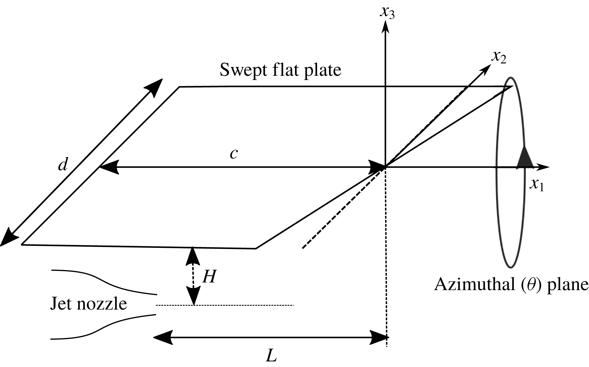
Reference Lyu, Dowling and Naqavi2017), the thickness and camber of the wing are neglected and the wing is therefore treated as a flat plate, as shown in figure 1. The flat plate has a swept trailing edge, with a mean chord
 $c$
and span
 $d$
, and is placed near a round jet nozzle. The centreline of the jet nozzle does not necessarily lie in the mid-span plane. However, as we will discuss in more detail in the rest of this paper, the nozzle does have to be sufficiently far away from either side edge of the flat plate, such that the side-edge scattering can be neglected. The bottom surface of the flat plate is
 $H$
above the jet centreline. The swept trailing edge is
 $L$
downstream from the jet nozzle exit, measured in the vertical plane containing the jet centreline. A Cartesian coordinate system has its origin fixed on the trailing edge in this vertical plane with
 $x_{1}$
in the streamwise direction,
 $x_{2}$
in the spanwise direction and
 $x_{3}$
in the direction normal to the plate. In this coordinate system, the swept trailing edge is specified by
 $x_{1}=F(x_{2})$
. Since the trailing edge is linearly swept,
 $$\begin{eqnarray}\displaystyle F(x_{2})=\unicode[STIX]{x1D70E}x_{2}, & & \displaystyle\end{eqnarray}$$
where
 $\unicode[STIX]{x1D70E}\equiv \tan \unicode[STIX]{x1D6FC}$
is a parameter specifying the sweep angle
 $\unicode[STIX]{x1D6FC}$
. In this coordinate system, the two side edges are located at
 $x_{3}=0,x_{2}=-l$
, where
 $0<l<d$
, and
 $x_{3}=0,x_{2}=d-l$
, respectively.
A schematic illustration of the simplified model problem.

As discussed in the earlier study, outside the jet there is a region of near-field pressure fluctuations, which are primarily induced by the jet’s hydrodynamic instability waves and decay exponentially in the radial direction (Jordan & Colonius Reference Jordan and Colonius2013). Because of this exponential decay, they contribute very weakly to the far-field sound. However, when a surface with sharp edges is present in the near field of the jet, the jet instability waves’ previously non-radiating pressure field can be efficiently scattered into sound by the edges. This is the primary physical mechanism of the observed noise intensification at low frequencies. Strictly speaking, when a flat plate is placed near the jet, the instability waves would be different from those of an isolated jet. However, as discussed in earlier works (Bychkov & Faranosov Reference Bychkov and Faranosov2014; Lyu et al.
Reference Lyu, Dowling and Naqavi2017), the influence of the flat plate on the instability characteristics is not significant provided
 $H$
is not so small as to significantly change the jet mean flow. We can therefore use the instability waves of an isolated jet as the input for the scattering problem considered in this paper. Note that the convection velocities of the instability waves of an isolated jet are found to be frequency dependent. For example, by analysing both large-eddy simulation (LES) and experimental data (Lyu & Dowling Reference Lyu and Dowling2017; Lyu et al.
Reference Lyu, Dowling and Naqavi2017) the convection velocity
 $U_{c}$
is found to be significantly lower than
 $0.6U_{j}$
at low frequencies (e.g.
 $St<0.1$
), where
 $U_{j}$
is the jet exit velocity.
We start to develop the model by assuming that the near-field pressure fluctuation is dominated by the evanescent wave of the first few azimuthal modes in the cylindrical coordinate system whose origin is on the jet centreline. As mentioned in § 1, the scattering mainly occurs in the local vicinity of the edge, and we may therefore neglect the axial growth, saturation and decay behaviour of the instability waves in the scattering process. The amplitude modulation may also contribute to the far-field sound directly through the wavenumber leakage (Tam & Viswanathan Reference Tam and Viswanathan2008; Jordan & Colonius Reference Jordan and Colonius2013), but this is much weaker than the scattered sound when the flat plate is placed close to the jet, in which this paper is particularly interested. We can therefore write the instability wave (omitting
 $\text{e}^{\text{i}\unicode[STIX]{x1D714}t}$
) near the swept edge as (for more detail see Lyu et al. (Reference Lyu, Dowling and Naqavi2017))
 $$\begin{eqnarray}\displaystyle p^{\prime }(\unicode[STIX]{x1D714},\boldsymbol{x})=\mathop{\sum }_{m=-N}^{N}\hat{p}(\unicode[STIX]{x1D714},m)K_{m}(\unicode[STIX]{x1D6FE}_{c}r)\text{e}^{-\text{i}k_{1}x_{1}}\text{e}^{\text{i}m\unicode[STIX]{x1D703}}, & & \displaystyle\end{eqnarray}$$
where
 $\hat{p}(\unicode[STIX]{x1D714},m)$
denotes the amplitude of the pressure fluctuations of mode
 $m$
and frequency
 $\unicode[STIX]{x1D714}$
,
 $K_{m}$
is the
 $m$
th-order modified Bessel function of the second kind,
 $k_{1}$
is the streamwise wavenumber of the instability waves and the radius
 $r$
here is now defined as
 $\sqrt{x_{2}^{2}+(x_{3}+H)^{2}}$
. Note that in practice the amplitude
 $\hat{p}(\unicode[STIX]{x1D714},m)$
can be obtained through pressure measurements in the near field of an isolated jet. We will discuss this in detail at the end of this section. The convection velocity
 $U_{c}$
(and hence
 $k_{1}$
) is a function of
 $\unicode[STIX]{x1D714}$
and
 $m$
. Angle
 $\unicode[STIX]{x1D703}$
is the azimuthal angle (measured from the
 $x_{3}$
axis in the clockwise direction) and
 $N$
is a small integer; for example, according to the LES data, we find
 $N=1$
is sufficient (Lyu & Dowling Reference Lyu and Dowling2016; Lyu et al.
Reference Lyu, Dowling and Naqavi2017). The convective radial decay rate
 $\unicode[STIX]{x1D6FE}_{c}$
, in the presence of ambient mean flow of Mach number
 $M_{a}$
, is given by (Amiet Reference Amiet1976; Lyu et al.
Reference Lyu, Dowling and Naqavi2017)
 $$\begin{eqnarray}\displaystyle \unicode[STIX]{x1D6FE}_{c}=\frac{\sqrt{(k_{1}\unicode[STIX]{x1D6FD}^{2}+kM_{a})^{2}-k^{2}}}{\unicode[STIX]{x1D6FD}}, & & \displaystyle\end{eqnarray}$$
where
 $\unicode[STIX]{x1D6FD}=\sqrt{1-M_{a}^{2}}$
and
 $k=\unicode[STIX]{x1D714}/c_{0}$
. We note here that (2.2) can also be written in terms of Hankel functions with an imaginary argument. But it can be shown that these two ways are equivalent to each other with appropriate choice of branch cut.
The jet instability waves will be scattered by the finite plate. However, when both side edges are sufficiently far away from the jet centreline, we can neglect the scattering of the instability waves by them (Lyu et al.
Reference Lyu, Dowling and Naqavi2017). This is possible because the jet instability waves decay exponentially in the radial direction, and hence the strength of these waves weakens sufficiently fast. As mentioned in the preceding section, in this study, the jet centreline does not have to be in the mid-span plane of the plate. But we do require both
 $l$
and
 $d-l$
to be large enough to justify this assumption. Therefore, in the following derivation, we neglect the contribution of side-edge scattering. A previous study has shown that the leading-edge backscattering of the trailing-edge noise of an aerofoil can be neglected when the frequency is sufficiently high, i.e. when
 $kc>1$
(Roger & Moreau Reference Roger and Moreau2005), and this is shown to be suitable for installed jet noise as well (Lyu et al.
Reference Lyu, Dowling and Naqavi2017). Therefore, in this study, we only take into account the scattering due to the sharp trailing edge of the swept plate.
When the flat plate is directly above the jet, the hypothetical incident pressure that would exist on the lower surface of the plate if the plate were absent is
 $$\begin{eqnarray}\displaystyle & & \displaystyle p_{h}(\unicode[STIX]{x1D714},x_{1},x_{2})=\mathop{\sum }_{m=-N}^{N}\hat{p}(\unicode[STIX]{x1D714},m)K_{m}(\unicode[STIX]{x1D6FE}_{c}\sqrt{x_{2}^{2}+H^{2}})\text{e}^{-\text{i}k_{1}x_{1}}\nonumber\\ \displaystyle & & \displaystyle \quad \times \left(\mathop{\sum }_{k=0}^{[|m|/2]}C_{|m|}^{2k}(-1)^{k}\frac{H^{|m|-2k}x_{2}^{2k}}{\sqrt{x_{2}^{2}+H^{2}}^{|m|}}+\text{i}\,\text{sgn}(m)\mathop{\sum }_{k=0}^{[(|m|-1)/2]}C_{|m|}^{2k+1}(-1)^{k}\frac{H^{|m|-2k-1}x_{2}^{2k+1}}{\sqrt{x_{2}^{2}+H^{2}}^{|m|}}\right),\nonumber\\ \displaystyle & & \displaystyle\end{eqnarray}$$
where
 $[x]$
means taking the nearest integer that is not larger than
 $x$
and
 $C_{m}^{n}$
is the binomial coefficient, which results from the use of de Moivre’s theorem. This hypothetical incident pressure can be decomposed into a superposition of a series of plane waves, namely
 $$\begin{eqnarray}\displaystyle p_{h}(\unicode[STIX]{x1D714},x_{1},x_{2})=\mathop{\sum }_{m=-N}^{N}\int _{-\infty }^{\infty }\tilde{p}(\unicode[STIX]{x1D714},k_{2},m)\text{e}^{-\text{i}(k_{1}x_{1}+k_{2}x_{2})}\,\text{d}k_{2}, & & \displaystyle\end{eqnarray}$$
where
 $$\begin{eqnarray}\displaystyle & & \displaystyle \tilde{p}(\unicode[STIX]{x1D714},k_{2},m)=\frac{1}{\sqrt{2\unicode[STIX]{x03C0}}}\hat{p}(\unicode[STIX]{x1D714},m)\nonumber\\ \displaystyle & & \displaystyle \quad \times \left\{\mathop{\sum }_{k=0}^{[|m|/2]}C_{|m|}^{2k}H^{-2k+1/2}\unicode[STIX]{x1D6FE}_{c}^{-|m|}\frac{\text{d}^{2k}}{\text{d}k_{2}^{2k}}[(\unicode[STIX]{x1D6FE}_{c}^{2}+k_{2}^{2})^{1/2|m|-1/4}K_{|m|-1/2}(H\sqrt{\unicode[STIX]{x1D6FE}_{c}^{2}+k_{2}^{2}})]-\text{sgn}(m)\right.\nonumber\\ \displaystyle & & \displaystyle \quad \times \left.\mathop{\sum }_{k=0}^{[(|m|-1)/2]}C_{|m|}^{2k+1}H^{-2k+1/2}\unicode[STIX]{x1D6FE}_{c}^{-|m|}\frac{\text{d}^{2k}}{\text{d}k_{2}^{2k}}[k_{2}(\unicode[STIX]{x1D6FE}_{c}^{2}+k_{2}^{2})^{1/2|m|-3/4}K_{|m|-3/2}(H\sqrt{\unicode[STIX]{x1D6FE}_{c}^{2}+k_{2}^{2}})]\right\}.\nonumber\\ \displaystyle & & \displaystyle\end{eqnarray}$$
For a plane-wave-like incident pressure given by
 $\tilde{p}(\unicode[STIX]{x1D714},k_{2},m)\text{e}^{-\text{i}(k_{1}x_{1}+k_{2}x_{2})}$
, the scattered pressure
 $p_{s}$
is governed by the convective wave equation (with ambient mean flow of Mach number
 $M_{a}$
)
 $$\begin{eqnarray}\displaystyle \unicode[STIX]{x1D6FD}^{2}\frac{\unicode[STIX]{x2202}^{2}p_{s}}{\unicode[STIX]{x2202}x_{1}^{2}}+\frac{\unicode[STIX]{x2202}^{2}p_{s}}{\unicode[STIX]{x2202}x_{2}^{2}}+\frac{\unicode[STIX]{x2202}^{2}p_{s}}{\unicode[STIX]{x2202}x_{3}^{2}}-2iM_{a}\frac{\unicode[STIX]{x2202}p_{s}}{\unicode[STIX]{x2202}x_{1}}+k^{2}p_{s}=0, & & \displaystyle\end{eqnarray}$$
subject to boundary conditions
 $$\begin{eqnarray}\displaystyle & p_{s}=-\tilde{p}\text{e}^{-\text{i}(k_{1}x_{1}+k_{2}x_{2})},\quad x_{1}>F(x_{2}) & \displaystyle\end{eqnarray}$$
 $$\begin{eqnarray}\displaystyle & \displaystyle \frac{\unicode[STIX]{x2202}p_{s}}{\unicode[STIX]{x2202}x_{3}}=0,\quad x_{1}<F(x_{2}). & \displaystyle\end{eqnarray}$$
With the coordinate transformation
 $x_{1}^{\prime }=x_{1}-F(x_{2})$
,
 $x_{2}^{\prime }=x_{2}$
and
 $x_{3}^{\prime }=\sqrt{\unicode[STIX]{x1D6FD}^{2}+\unicode[STIX]{x1D70E}^{2}}x_{3}$
and the new variable definition
 $\unicode[STIX]{x1D719}=p_{s}\text{e}^{\text{i}\bar{k}_{2}x_{2}^{\prime }}\text{e}^{\text{i}(\bar{k}_{2}\unicode[STIX]{x1D70E}-kM_{a})/(\unicode[STIX]{x1D6FD}^{2}+\unicode[STIX]{x1D70E}^{2})x_{1}^{\prime }}$
, where
 $\bar{k}_{2}=k_{2}+k_{1}\unicode[STIX]{x1D70E}$
, the governing equation reduces to
 $$\begin{eqnarray}\displaystyle \frac{\unicode[STIX]{x2202}^{2}\unicode[STIX]{x1D719}}{\unicode[STIX]{x2202}{x_{1}^{\prime }}^{2}}+\frac{\unicode[STIX]{x2202}^{2}\unicode[STIX]{x1D719}}{\unicode[STIX]{x2202}{x_{3}^{\prime }}^{2}}+K^{2}\unicode[STIX]{x1D719}=0, & & \displaystyle\end{eqnarray}$$
where
 $$\begin{eqnarray}\displaystyle K=\frac{\sqrt{k^{2}-\bar{k}_{2}^{2}+(\bar{k}_{2}M_{a}-k\unicode[STIX]{x1D70E})^{2}}}{\unicode[STIX]{x1D6FD}^{2}+\unicode[STIX]{x1D70E}^{2}}. & & \displaystyle\end{eqnarray}$$
The boundary conditions now read
 $$\begin{eqnarray}\displaystyle & \unicode[STIX]{x1D719}=-\tilde{p}\text{e}^{-\text{i}k_{1}x_{1}^{\prime }}\text{e}^{\text{i}(\bar{k}_{2}\unicode[STIX]{x1D70E}-kM_{a})/(\unicode[STIX]{x1D6FD}^{2}+\unicode[STIX]{x1D70E}^{2})x_{1}^{\prime }},\quad x_{1}^{\prime }>0 & \displaystyle\end{eqnarray}$$
 $$\begin{eqnarray}\displaystyle & \displaystyle \frac{\unicode[STIX]{x2202}\unicode[STIX]{x1D719}}{\unicode[STIX]{x2202}x_{3}^{\prime }}=0,\quad x_{1}^{\prime }<0. & \displaystyle\end{eqnarray}$$
The solution to (2.10) can be readily found using the Schwarzchild technique (Lyu, Azarpeyvand & Sinayoko Reference Lyu, Azarpeyvand and Sinayoko2016; Lyu et al. Reference Lyu, Dowling and Naqavi2017). By transforming back to the original coordinate system, one can show that the scattered pressure is
 $$\begin{eqnarray}\displaystyle p_{s}=\tilde{p}(\unicode[STIX]{x1D714},k_{2},m)\text{e}^{-\text{i}(k_{1}x_{1}+k_{2}x_{2})}[(1+\text{i})E_{0}(-\unicode[STIX]{x1D707}(x_{1}-\unicode[STIX]{x1D70E}x_{2}))-1], & & \displaystyle\end{eqnarray}$$
where
 $$\begin{eqnarray}\displaystyle \unicode[STIX]{x1D707}=k_{1}+\frac{(kM_{a}-\bar{k}_{2}\unicode[STIX]{x1D70E})}{\unicode[STIX]{x1D6FD}^{2}+\unicode[STIX]{x1D70E}^{2}}+\frac{\sqrt{k^{2}-\bar{k}_{2}^{2}+(\bar{k}_{2}M_{a}-k\unicode[STIX]{x1D70E})^{2}}}{\unicode[STIX]{x1D6FD}^{2}+\unicode[STIX]{x1D70E}^{2}},\quad E_{0}(x)=\int _{0}^{x}\frac{\text{e}^{-\text{i}t}}{\sqrt{2\unicode[STIX]{x03C0}t}}\,\text{d}t. & & \displaystyle \nonumber\\ \displaystyle & & \displaystyle\end{eqnarray}$$
Equation (2.14) shows that the scattered surface pressure has a phase variation along the spanwise (
 $x_{2}$
) direction even when
 $k_{2}=0$
due to the
 $x_{2}$
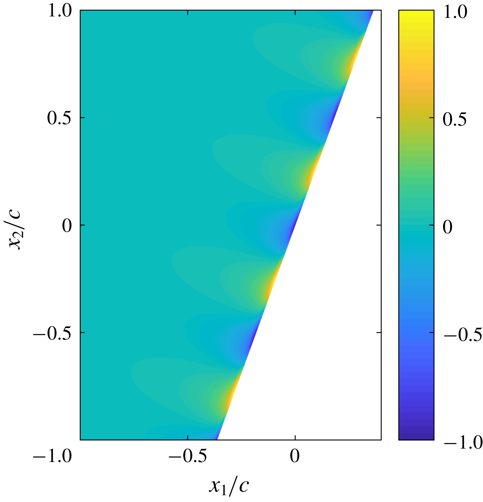
dependence in the square bracket, which does not occur in the case of a straight trailing edge. To show this more clearly, we have plotted a typical pressure distribution on the surface of a swept flat plate according to the real part of (2.14) in figure 2 for a plane-wave-like incident pressure
 $\tilde{p}(\unicode[STIX]{x1D714},k_{2},m)\text{e}^{-\text{i}(k_{1}x_{1}+k_{2}x_{2})}$
with
 $k_{2}=0$
. The phase variation along the trailing edge of the flat plate can be clearly observed. The theory of Curle (Reference Curle1955) shows that the scattered surface pressure acts like a distribution of dipole sources, and the far-field sound can be obtained by calculating the sound generated from this distribution of dipole sources. The substantial phase variation exhibited by figure 2 implies that some of these dipole sources are in anti-phase and would result in destructive (can also be constructive depending on the position of the observer) interference, which, as will be discussed in detail in the rest of this paper, is the primary mechanism of installed jet noise reduction observed in the experiments.
The scattered pressure on the surface of a swept flat plate induced by a plane-wave-like incident pressure. The contour is obtained from the real part of (2.14) with
 $\tilde{p}=1$
,
 $kc=10$
,
 $k_{2}=0$
,
 $M_{a}=0$
,
 $M=0.5$
,
 $U_{c}=0.6U_{j}$
and
 $\unicode[STIX]{x1D6FC}=20^{\circ }$
.

Because of linearity, the far-field sound induced by the incident pressure given by (2.5) can be readily calculated according to the theory of Kirchhoff and Curle (Lyu et al. Reference Lyu, Azarpeyvand and Sinayoko2016; Lyu & Dowling Reference Lyu and Dowling2017) to be
 $$\begin{eqnarray}\displaystyle p_{f}(\unicode[STIX]{x1D714},\boldsymbol{x}) & = & \displaystyle (1+\text{i})\frac{\unicode[STIX]{x1D714}x_{3}}{\unicode[STIX]{x03C0}c_{0}S_{0}^{2}}\text{e}^{\text{i}(k/\unicode[STIX]{x1D6FD}^{2})(M_{a}x_{1}-S_{0})}\nonumber\\ \displaystyle & & \displaystyle \times \mathop{\sum }_{m=-N}^{N}\int _{-\infty }^{\infty }\text{e}^{\text{i}\unicode[STIX]{x1D705}(l-d/2)}\frac{\sin [\unicode[STIX]{x1D705}d/2]}{\unicode[STIX]{x1D705}}\frac{1}{\unicode[STIX]{x1D707}_{A}}\unicode[STIX]{x1D6E4}(c,\unicode[STIX]{x1D707},\unicode[STIX]{x1D707}_{A})\tilde{p}(\unicode[STIX]{x1D714},k_{2},m)\,\text{d}k_{2},\end{eqnarray}$$
where
 $\unicode[STIX]{x1D705}=\bar{k}_{2}-kx_{2}/S_{0}-(k/\unicode[STIX]{x1D6FD}^{2})(x_{1}/S_{0}-M_{a})\unicode[STIX]{x1D70E}$
,
 $x_{1}$
,
 $x_{2}$
and
 $x_{3}$
now denote the Cartesian coordinates of the far-field observer, and the properly bounded function
 $\unicode[STIX]{x1D6E4}$
in (2.16) is defined as
 $$\begin{eqnarray}\displaystyle \unicode[STIX]{x1D6E4}(x,\unicode[STIX]{x1D707},\unicode[STIX]{x1D707}_{A})=\text{e}^{\text{i}\unicode[STIX]{x1D707}_{A}x}E_{0}(\unicode[STIX]{x1D707}x)-\sqrt{\frac{\unicode[STIX]{x1D707}}{\unicode[STIX]{x1D707}-\unicode[STIX]{x1D707}_{A}}}E_{0}[(\unicode[STIX]{x1D707}-\unicode[STIX]{x1D707}_{A})x]+\frac{1}{1+\text{i}}(1-\text{e}^{\text{i}\unicode[STIX]{x1D707}_{A}x}), & & \displaystyle\end{eqnarray}$$
where
 $$\begin{eqnarray}\displaystyle \left.\begin{array}{@{}c@{}}\displaystyle S_{0}=\sqrt{x_{1}^{2}+\unicode[STIX]{x1D6FD}^{2}(x_{2}^{2}+x_{3}^{2})},\\ \displaystyle \unicode[STIX]{x1D707}_{A}=k_{1}+\frac{k}{\unicode[STIX]{x1D6FD}^{2}}\left(M_{a}-\frac{x_{1}}{S_{0}}\right).\end{array}\right\} & & \displaystyle\end{eqnarray}$$
In reaching (2.16), we have made a simplification by assuming that the leading edge is also swept by an angle of
 $\unicode[STIX]{x1D6FC}$
. This is permissible because, as mentioned earlier, the leading-edge backscattering is weak enough to be neglected. Consequently, replacing a straight leading edge with a swept one should cause minimal change to the far-field sound. It should be noted that (2.16) is due to the contribution of the scattered pressure only. In order to take the incident wave contribution into consideration, the term 1 in the last parentheses on the right-hand side of (2.17) defining the function
 $\unicode[STIX]{x1D6E4}(x,\unicode[STIX]{x1D707},\unicode[STIX]{x1D707}_{A})$
should be omitted (Amiet Reference Amiet1978).
Equation (2.16) can be further simplified by noting that normally aircraft wings have a large span-to-chord ratio, and
 $d$
can be quite large compared to the sound wavelength at the frequency of peak noise enhancement in the low-frequency regime. Therefore we use
 $$\begin{eqnarray}\displaystyle \lim _{d\rightarrow \infty }\frac{\sin [\unicode[STIX]{x1D705}d/2]}{\unicode[STIX]{x03C0}\unicode[STIX]{x1D705}}=\unicode[STIX]{x1D6FF}(\unicode[STIX]{x1D705}) & & \displaystyle\end{eqnarray}$$
to simplify (2.16) to
 $$\begin{eqnarray}\displaystyle p_{f}(\unicode[STIX]{x1D714},\boldsymbol{x})=(1+\text{i})\frac{\unicode[STIX]{x1D714}x_{3}}{c_{0}S_{0}^{2}}\text{e}^{\text{i}(k/\unicode[STIX]{x1D6FD}^{2})(M_{a}x_{1}-S_{0})}\mathop{\sum }_{m=-N}^{N}\frac{1}{\unicode[STIX]{x1D707}_{A}}\unicode[STIX]{x1D6E4}(c,\unicode[STIX]{x1D707}_{o},\unicode[STIX]{x1D707}_{A})\tilde{p}(\unicode[STIX]{x1D714},k_{o},m), & & \displaystyle\end{eqnarray}$$
where
 $k_{o}=-k_{1}\unicode[STIX]{x1D70E}+kx_{2}/S_{0}+(k/\unicode[STIX]{x1D6FD}^{2})(x_{1}/S_{0}-M_{a})\unicode[STIX]{x1D70E}$
and
 $\unicode[STIX]{x1D707}_{o}=\unicode[STIX]{x1D707}|_{k_{2}=k_{o}}$
. We see that when the span is large, an effective destructive interference along the span is possible and (2.20) shows that only the plane wave with a spanwise wavenumber
 $k_{o}$
can be heard in the far field. Plane waves with other values of
 $k_{2}$
do not contribute to the far-field sound due to effective destructive interference (see figure 2 for the example of
 $k_{2}=0$
). However, the validity of this result hinges on the assumption of a sufficiently long span, which is used to obtain (2.19) and (2.20). Therefore, it is expected that a longer span is required for it to be valid at lower frequencies. Note that
 $l$
does not enter (2.20). This implies that, provided side-edge scattering can be neglected, the far-field sound is not sensitive to the spanwise position of the plate relative to the jet nozzle.
The far-field sound power spectrum can be found by formulating the ensemble average to be
 $$\begin{eqnarray}\displaystyle \unicode[STIX]{x1D6F7}_{N}(\unicode[STIX]{x1D714},\boldsymbol{x}) & = & \displaystyle 2\left[\frac{\unicode[STIX]{x1D714}x_{3}}{c_{0}S_{0}^{2}}\right]^{2}\mathop{\sum }_{m=-N}^{N}\mathop{\sum }_{m^{\prime }=-N}^{N}\left.\frac{\unicode[STIX]{x1D6E4}(c,\unicode[STIX]{x1D707}_{o},\unicode[STIX]{x1D707}_{A})}{\unicode[STIX]{x1D707}_{A}}\right|_{m}\left.\frac{\unicode[STIX]{x1D6E4}^{\ast }(c,\unicode[STIX]{x1D707}_{o},\unicode[STIX]{x1D707}_{A})}{\unicode[STIX]{x1D707}_{A}^{\ast }}\right|_{m^{\prime }}\nonumber\\ \displaystyle & & \displaystyle \times \,\lim _{T\rightarrow \infty }\frac{\unicode[STIX]{x03C0}}{T}\,\overline{\tilde{p}(\unicode[STIX]{x1D714},k_{o},m)\tilde{p}^{\ast }(\unicode[STIX]{x1D714},k_{o},m^{\prime })},\end{eqnarray}$$
where
 $2T$
(Amiet Reference Amiet1975) is the temporal interval used to perform the Fourier transformation to obtain
 $p_{f}(\unicode[STIX]{x1D714},\boldsymbol{x})$
and the overbar denotes ensemble average. We note that (2.21) is the result obtained using Amiet’s approach where the interval of Fourier transformation is finite. When the interval is infinite, we have (Dowling & Williams Reference Dowling and Williams1983; Howe Reference Howe1991)
 $$\begin{eqnarray}\displaystyle \unicode[STIX]{x1D6F7}_{N}(\unicode[STIX]{x1D714},\boldsymbol{x})=\int _{-\infty }^{\infty }\overline{p_{f}(\unicode[STIX]{x1D714},\boldsymbol{x})p_{f}^{\ast }(\unicode[STIX]{x1D714}^{\prime },\boldsymbol{x})}\,\text{d}\unicode[STIX]{x1D714}^{\prime }. & & \displaystyle\end{eqnarray}$$
The two approaches, however, yield identical answers for statistically stationary signals, and we use the former one in this paper.
Substituting (2.6) into the above equation yields
 $$\begin{eqnarray}\displaystyle & & \displaystyle \unicode[STIX]{x1D6F7}_{N}(\unicode[STIX]{x1D714},\boldsymbol{x})=\frac{1}{\unicode[STIX]{x03C0}}\left[\frac{\unicode[STIX]{x1D714}x_{3}}{c_{0}S_{0}^{2}}\right]^{2}\mathop{\sum }_{m=-N}^{N}\left|\frac{\unicode[STIX]{x1D6E4}(c,\unicode[STIX]{x1D707}_{o},\unicode[STIX]{x1D707}_{A})}{\unicode[STIX]{x1D707}_{A}}\right|^{2}\unicode[STIX]{x1D6F1}(\unicode[STIX]{x1D714},m)\nonumber\\ \displaystyle & & \displaystyle \quad \times \left\{\mathop{\sum }_{k=0}^{[|m|/2]}C_{|m|}^{2k}H^{-2k+1/2}\unicode[STIX]{x1D6FE}_{c}^{-|m|}\frac{\text{d}^{2k}}{\text{d}k_{o}^{2k}}[(\unicode[STIX]{x1D6FE}_{c}^{2}+k_{o}^{2})^{1/2|m|-1/4}K_{|m|-1/2}(H\sqrt{\unicode[STIX]{x1D6FE}_{c}^{2}+k_{o}^{2}})]-\text{sgn}(m)\right.\nonumber\\ \displaystyle & & \displaystyle \quad \times \left.\mathop{\sum }_{k=0}^{[(|m|-1)/2]}C_{|m|}^{2k+1}H^{-2k+1/2}\unicode[STIX]{x1D6FE}_{c}^{-|m|}\frac{\text{d}^{2k}}{\text{d}k_{o}^{2k}}[k_{o}(\unicode[STIX]{x1D6FE}_{c}^{2}+k_{o}^{2})^{1/2|m|-3/4}K_{|m|-3/2}(H\sqrt{\unicode[STIX]{x1D6FE}_{c}^{2}+k_{o}^{2}})]\right\}^{2},\nonumber\\ \displaystyle & & \displaystyle\end{eqnarray}$$
where
 $\unicode[STIX]{x1D6F1}(\unicode[STIX]{x1D714},m)$
denotes the power spectrum of
 $m$
th-order near-field evanescent waves and is given by
 $\unicode[STIX]{x1D6F1}(\unicode[STIX]{x1D714},m)=\lim _{T\rightarrow \infty }(\unicode[STIX]{x03C0}/T)\overline{\hat{p}(\unicode[STIX]{x1D714},m)\hat{p}^{\ast }(\unicode[STIX]{x1D714},m)}$
with
 $2T$
being the temporal interval of the Fourier transformation used to obtain
 $\hat{p}(\unicode[STIX]{x1D714},m)$
. Similar to (2.22),
 $\unicode[STIX]{x1D6F1}(\unicode[STIX]{x1D714},m)$
can also be formulated as
 $\unicode[STIX]{x1D6F1}(\unicode[STIX]{x1D714},m)=\int _{-\infty }^{\infty }\overline{\hat{p}(\unicode[STIX]{x1D714},m)\hat{p}^{\ast }(\unicode[STIX]{x1D714}^{\prime },m)}\,\text{d}\unicode[STIX]{x1D714}^{\prime }$
. Equation (2.23) is the generic form of near-field scattering model. However, further simplifications can be made in practical cases. First, if we assume that the fluctuation is symmetric with respect to
 $m$
, i.e.
 $\unicode[STIX]{x1D6F1}(\unicode[STIX]{x1D714},m)=\unicode[STIX]{x1D6F1}(\unicode[STIX]{x1D714},-m)$
, equation (2.23) can be further simplified to
 $$\begin{eqnarray}\displaystyle & & \displaystyle \unicode[STIX]{x1D6F7}_{N}(\unicode[STIX]{x1D714},\boldsymbol{x})=\frac{1}{\unicode[STIX]{x03C0}}\left[\frac{\unicode[STIX]{x1D714}x_{3}}{c_{0}S_{0}^{2}}\right]^{2}\mathop{\sum }_{m=0}^{N}\left|\frac{\unicode[STIX]{x1D6E4}(c,\unicode[STIX]{x1D707}_{o},\unicode[STIX]{x1D707}_{A})}{\unicode[STIX]{x1D707}_{A}}\right|^{2}\unicode[STIX]{x1D6F1}_{s}(\unicode[STIX]{x1D714},m)\nonumber\\ \displaystyle & & \displaystyle \quad \times \left\{\!\left(\mathop{\sum }_{k=0}^{[|m|/2]}C_{|m|}^{2k}H^{-2k+1/2}\unicode[STIX]{x1D6FE}_{c}^{-|m|}\frac{\text{d}^{2k}}{\text{d}k_{o}^{2k}}[(\unicode[STIX]{x1D6FE}_{c}^{2}+k_{o}^{2})^{1/2|m|-1/4}K_{|m|-1/2}(H\sqrt{\unicode[STIX]{x1D6FE}_{c}^{2}+k_{o}^{2}})]\right)^{2}\right.\nonumber\\ \displaystyle & & \displaystyle \quad +\left.\left(\mathop{\sum }_{k=0}^{[|m|-1/2]}C_{|m|}^{2k+1}H^{-2k+1/2}\unicode[STIX]{x1D6FE}_{c}^{-|m|}\frac{\text{d}^{2k}}{\text{d}k_{o}^{2k}}[k_{o}(\unicode[STIX]{x1D6FE}_{c}^{2}+k_{o}^{2})^{1/2|m|-3/4}K_{|m|-3/2}(H\sqrt{\unicode[STIX]{x1D6FE}_{c}^{2}+k_{o}^{2}})]\right)^{2}\right\},\nonumber\\ \displaystyle & & \displaystyle\end{eqnarray}$$
where
 $\unicode[STIX]{x1D6F1}_{s}(\unicode[STIX]{x1D714},m)$
is
 $m$
th single-sided modal PSD, i.e.
 $\unicode[STIX]{x1D6F1}_{s}(\unicode[STIX]{x1D714},m)=\unicode[STIX]{x1D6F1}(\unicode[STIX]{x1D714},m)+\unicode[STIX]{x1D6F1}(\unicode[STIX]{x1D714},-m)$
for
 $m\neq 0$
. If we assume that only the
 $0$
and
 $1(-1)$
modes are significant, we can show the far-field sound spectral density in a simplified form as
 $$\begin{eqnarray}\displaystyle \unicode[STIX]{x1D6F7}_{N}(\unicode[STIX]{x1D714},\boldsymbol{x})\approx {\mathcal{H}}_{0}(\unicode[STIX]{x1D714},\boldsymbol{x})\unicode[STIX]{x1D6F1}_{s}(\unicode[STIX]{x1D714},0)+{\mathcal{H}}_{1}(\unicode[STIX]{x1D714},\boldsymbol{x})\unicode[STIX]{x1D6F1}_{s}(\unicode[STIX]{x1D714},1), & & \displaystyle\end{eqnarray}$$
where
 $$\begin{eqnarray}\displaystyle & \displaystyle {\mathcal{H}}_{0}(\unicode[STIX]{x1D714},\boldsymbol{x})=\left[\frac{\unicode[STIX]{x1D714}x_{3}}{c_{0}S_{0}^{2}}\right]^{2}\left\{\left|\frac{\unicode[STIX]{x1D6E4}(c,\unicode[STIX]{x1D707}_{o},\unicode[STIX]{x1D707}_{A})}{\unicode[STIX]{x1D707}_{A}}\right|^{2}\frac{\text{e}^{-2H\sqrt{\unicode[STIX]{x1D6FE}_{c}^{2}+k_{o}^{2}}}}{2(\unicode[STIX]{x1D6FE}_{c}^{2}+k_{o}^{2})}\right\}_{m=0}, & \displaystyle\end{eqnarray}$$
 $$\begin{eqnarray}\displaystyle & \displaystyle {\mathcal{H}}_{1}(\unicode[STIX]{x1D714},\boldsymbol{x})=\left[\frac{\unicode[STIX]{x1D714}x_{3}}{c_{0}S_{0}^{2}}\right]^{2}\left\{\left|\frac{\unicode[STIX]{x1D6E4}(c,\unicode[STIX]{x1D707}_{o},\unicode[STIX]{x1D707}_{A})}{\unicode[STIX]{x1D707}_{A}}\right|^{2}\frac{\text{e}^{-2H\sqrt{\unicode[STIX]{x1D6FE}_{c}^{2}+k_{o}^{2}}}}{2\unicode[STIX]{x1D6FE}_{c}^{2}}\left(1+\frac{k_{o}^{2}}{k_{o}^{2}+\unicode[STIX]{x1D6FE}_{c}^{2}}\right)\right\}_{m=1}. & \displaystyle\end{eqnarray}$$
In the above equations, the near-field pressure spectra
 $\unicode[STIX]{x1D6F1}_{s}(\unicode[STIX]{x1D714},m)$
need to be known in order to predict the far-field sound PSD. These spectra could be obtained from simple models validated by experiments or LES simulations. Let
 $\unicode[STIX]{x1D6F1}_{0}(\unicode[STIX]{x1D714},0)$
and
 $\unicode[STIX]{x1D6F1}_{0}(\unicode[STIX]{x1D714},1)$
denote the zeroth- and first-order single-sided modal PSDs measured at a location of
 $r=r_{0}$
in the near field of the jet. Then it follows that
 $\unicode[STIX]{x1D6F1}_{s}(\unicode[STIX]{x1D714},0)=\unicode[STIX]{x1D6F1}_{0}(\unicode[STIX]{x1D714},0)/K_{0}^{2}(\unicode[STIX]{x1D6FE}_{c}r_{0})$
and
 $\unicode[STIX]{x1D6F1}_{s}(\unicode[STIX]{x1D714},1)=\unicode[STIX]{x1D6F1}_{0}(\unicode[STIX]{x1D714},1)/K_{1}^{2}(\unicode[STIX]{x1D6FE}_{c}r_{0})$
. Therefore, the input of this model can be found by measuring the near-field pressure fluctuations using at least two microphones (to resolve mode 0 and mode 1) at suitable radial locations. To ensure that acoustic fluctuations are negligible, one must choose
 $r_{0}$
to be small such that the microphones are sufficiently close to the jet. Since near-field pressure spectra vary with axial position, it is desirable to put the microphones at the position where the trailing edge of the flat plate would be (in the mid-span plane) if a swept flat plate were to be present, i.e. the place where the incident wave is to be scattered most strongly.
3 Discussion
The transfer functions
 ${\mathcal{H}}_{0}(\unicode[STIX]{x1D714},\boldsymbol{x})$
and
 ${\mathcal{H}}_{1}(\unicode[STIX]{x1D714},\boldsymbol{x})$
determine how the near-field hydrodynamic pressure is scattered into sound. To understand the physical mechanism of the aforementioned sound reduction, it suffices to examine these two transfer functions. Since the transfer functions also contain the directivity terms, for simplicity one can examine their behaviour at a fixed observer position. If needed, similar analytical approaches can be followed for other observer points. For example, one can choose the observer to be at
 $90^{\circ }$
directly above the trailing edge in the mid-span plane, i.e. the observer is located at
 $(0,0,x_{3})$
. Then one can see that, for fixed frequencies,
 $$\begin{eqnarray}\displaystyle & \displaystyle {\mathcal{H}}_{0}(\unicode[STIX]{x1D714},\boldsymbol{x})\sim \left\{|\unicode[STIX]{x1D6E4}(c,\unicode[STIX]{x1D707}_{o},\unicode[STIX]{x1D707}_{A})|^{2}\frac{\text{e}^{-2H\sqrt{\unicode[STIX]{x1D6FE}_{c}^{2}+k_{o}^{2}}}}{2(\unicode[STIX]{x1D6FE}_{c}^{2}+k_{o}^{2})}\right\}_{m=0}, & \displaystyle\end{eqnarray}$$
 $$\begin{eqnarray}\displaystyle & \displaystyle {\mathcal{H}}_{1}(\unicode[STIX]{x1D714},\boldsymbol{x})\sim \left\{|\unicode[STIX]{x1D6E4}(c,\unicode[STIX]{x1D707}_{o},\unicode[STIX]{x1D707}_{A})|^{2}\frac{\text{e}^{-2H\sqrt{\unicode[STIX]{x1D6FE}_{c}^{2}+k_{o}^{2}}}}{2\unicode[STIX]{x1D6FE}_{c}^{2}}\left(1+\frac{k_{o}^{2}}{k_{o}^{2}+\unicode[STIX]{x1D6FE}_{c}^{2}}\right)\right\}_{m=1}, & \displaystyle\end{eqnarray}$$
where
 $$\begin{eqnarray}\displaystyle & \displaystyle k_{o}=-\left(k_{1}+\frac{kM_{a}}{\unicode[STIX]{x1D6FD}^{2}}\right)\unicode[STIX]{x1D70E}, & \displaystyle\end{eqnarray}$$
 $$\begin{eqnarray}\displaystyle & \displaystyle \unicode[STIX]{x1D707}_{o}=k_{1}+\frac{kM_{a}}{\unicode[STIX]{x1D6FD}^{2}}+k\frac{\sqrt{1-(M_{a}\unicode[STIX]{x1D70E}/\unicode[STIX]{x1D6FD}^{2})^{2}+(M_{a}^{2}\unicode[STIX]{x1D70E}/\unicode[STIX]{x1D6FD}^{2}+\unicode[STIX]{x1D70E})^{2}}}{\unicode[STIX]{x1D6FD}^{2}+\unicode[STIX]{x1D70E}^{2}}. & \displaystyle\end{eqnarray}$$
From the discussion in the preceding section, we can interpret the scattering process as a two-step process. First, the swept trailing edge selects the dominant plane-wave mode (because other plane-wave modes would result in no sound due to destructive interference). The strength of this selected mode is specified by the second product term in
 ${\mathcal{H}}_{0}(\unicode[STIX]{x1D714},\boldsymbol{x})$
and
 ${\mathcal{H}}_{1}(\unicode[STIX]{x1D714},\boldsymbol{x})$
. In the second step, the selected plane-wave mode is scattered into sound by the trailing edge. The scattering efficiency is determined by the first product term in the transfer functions. Therefore, by evaluating how these two terms differ from those for a straight trailing edge, the mechanism of the sound reduction can be readily made evident.
We start from the first selection step. Examining the second product term in
 ${\mathcal{H}}_{0}(\unicode[STIX]{x1D714},\boldsymbol{x})$
, we can see that the term contains both an exponential and an algebraic decay as
 $\unicode[STIX]{x1D70E}$
increases. However, since
 $\unicode[STIX]{x1D6FE}_{c}\sim k_{1}$
and
 $k_{o}\sim k_{1}\unicode[STIX]{x1D70E}$
, we see that this increase would only be significant when
 $\unicode[STIX]{x1D70E}\sim O(1)$
(because for
 $\unicode[STIX]{x1D70E}\ll 1$
, the leading order of the exponential decay is
 ${\sim}\text{e}^{-k_{1}H\unicode[STIX]{x1D70E}^{2}}$
). In other words, the sweep angle should be large enough in order to see a difference caused by this decay. For example, a negligible decay can be expected if
 $\unicode[STIX]{x1D6FC}\sim 10^{\circ }$
. A similar conclusion can be made for the transfer function
 ${\mathcal{H}}_{1}(\unicode[STIX]{x1D714},\boldsymbol{x})$
. A slight difference is that as
 $\unicode[STIX]{x1D70E}$
increases, there exists not only an exponential decay but also an algebraic growth. One can show that the algebraic term is the contribution of the
 $\sin \unicode[STIX]{x1D703}$
mode of the first-order instability wave. When the trailing edge is not swept,
 $k_{o}=0$
, the contribution of the
 $\sin \unicode[STIX]{x1D703}$
mode is zero in the mid-span plane. This is to be expected because the
 $\sin \unicode[STIX]{x1D703}$
mode is antisymmetric with respect to the mid-span plane and hence induces an antisymmetric scattered pressure field. A swept trailing edge, however, breaks this symmetry hence the
 $\sin \unicode[STIX]{x1D703}$
mode also contributes to the far-field sound. Nevertheless, when
 $k_{1}H$
and
 $\unicode[STIX]{x1D70E}$
are sufficiently large we expect the exponential decay term to be dominant. We can verify that when
 $\unicode[STIX]{x1D70E}\rightarrow O(1)$
this is indeed the case for the frequency of range of interest (for example
 $0.03<St<0.3$
).
Examining the
 $\unicode[STIX]{x1D6E4}$
functions can reveal how the scattering efficiency changes. As
 $\unicode[STIX]{x1D70E}$
changes from 0 to finite values,
 $\unicode[STIX]{x1D707}_{o}$
changes from
 $$\begin{eqnarray}\displaystyle k_{1}+\frac{kM_{a}}{\unicode[STIX]{x1D6FD}^{2}}+\frac{k}{\unicode[STIX]{x1D6FD}^{2}} & & \displaystyle\end{eqnarray}$$
to
 $$\begin{eqnarray}\displaystyle k_{1}+\frac{kM_{a}}{\unicode[STIX]{x1D6FD}^{2}}+k\frac{\sqrt{1-(M_{a}\unicode[STIX]{x1D70E}/\unicode[STIX]{x1D6FD}^{2})^{2}+(M_{a}^{2}\unicode[STIX]{x1D70E}/\unicode[STIX]{x1D6FD}^{2}+\unicode[STIX]{x1D70E})^{2}}}{\unicode[STIX]{x1D6FD}^{2}+\unicode[STIX]{x1D70E}^{2}}. & & \displaystyle\end{eqnarray}$$
Since the scattering of instability waves is only relevant at low frequencies, e.g.
 $St<0.3$
, where the convection velocities of the instability waves are significantly lower than
 $0.6U_{j}$
, we can show that
 $k_{1}\gg k$
. Hence the change of
 $\unicode[STIX]{x1D70E}$
from 0 to
 $O(1)$
values does not alter the values of
 $\unicode[STIX]{x1D707}_{o}$
significantly. Besides, all the terms contained in the function
 $\unicode[STIX]{x1D6E4}(c,\unicode[STIX]{x1D707}_{o},\unicode[STIX]{x1D707}_{A})$
have at most algebraic growth or decay. We can therefore expect an insignificant change to the scattering efficiency.
In summary, we see that most of the sound reduction is due to the selection process. Since the mechanism of this selection process is due to destructive interference, the principal mechanism of sound reduction by using swept trailing edges is therefore destructive interference.
4 Results
Using (2.25), both the spectra and the directivity patterns of the far-field sound can be readily plotted. Since the model needs an input of the near-field pressure spectra, in this paper we use the spectra measured in the experiment carried out by the authors in an earlier study (Lyu & Dowling Reference Lyu and Dowling2017, Reference Lyu and Dowling2018). This experiment was carried out in the anechoic chamber at the Engineering Department at the University of Cambridge, where a round, cold, Mach 0.5 jet of diameter 2.54 cm was operated both with and without a nearby flat plate. For a detailed description of the experimental set-up used to measure the near-field pressure spectra, readers are referred to earlier works (Lyu & Dowling Reference Lyu and Dowling2017, Reference Lyu and Dowling2018).
In the following, we present the far-field sound spectra first. As a starting point, we focus on a Mach 0.5 jet, where installed jet noise tends to be more significant than a jet of higher speed (Lyu et al. Reference Lyu, Dowling and Naqavi2017). The speed of a Mach 0.5 jet is relevant to the landing configurations of a modern aircraft, where engines are operated in a low-power mode. However, it is worth noting that the model is not restricted by specific jet speeds, and it would work with any Mach number provided the underlying scattering physics remains unchanged. As mentioned in § 1, installed jet noise contains two parts, one due to the scattering of instability waves and the other due to the scattering of Lighthill’s quadrupole sources. Although we are primarily interested in the scattering of the instability waves at low frequencies, it is useful to be able to quantify the relative contribution of the quadrupole sources, especially for the case of swept edges. To give an example, we can consider the following case. If the swept edge were to result in a substantial noise reduction, the far-field sound could be dominated by the quadrupoles’ contribution and the practical noise reduction one can observe in experiments would not be as large as that predicted by the reduced scattering of instability waves. Hence in the following figures, we plot the total sound spectra in the far field by adding the instability-scattering spectra to that due to the scattering of quadrupole sources by a straight trailing edge from earlier work (Lyu & Dowling Reference Lyu and Dowling2017). Note that the contribution of the quadrupole sources for the straight-edge case is only added in for reference, and our primary interest is to evaluate the changes to the instability-scattering spectra due to the use of swept edges. A more detailed discussion of the difference of quadrupole scattering by a straight and a swept trailing edge is given at the end of this section.
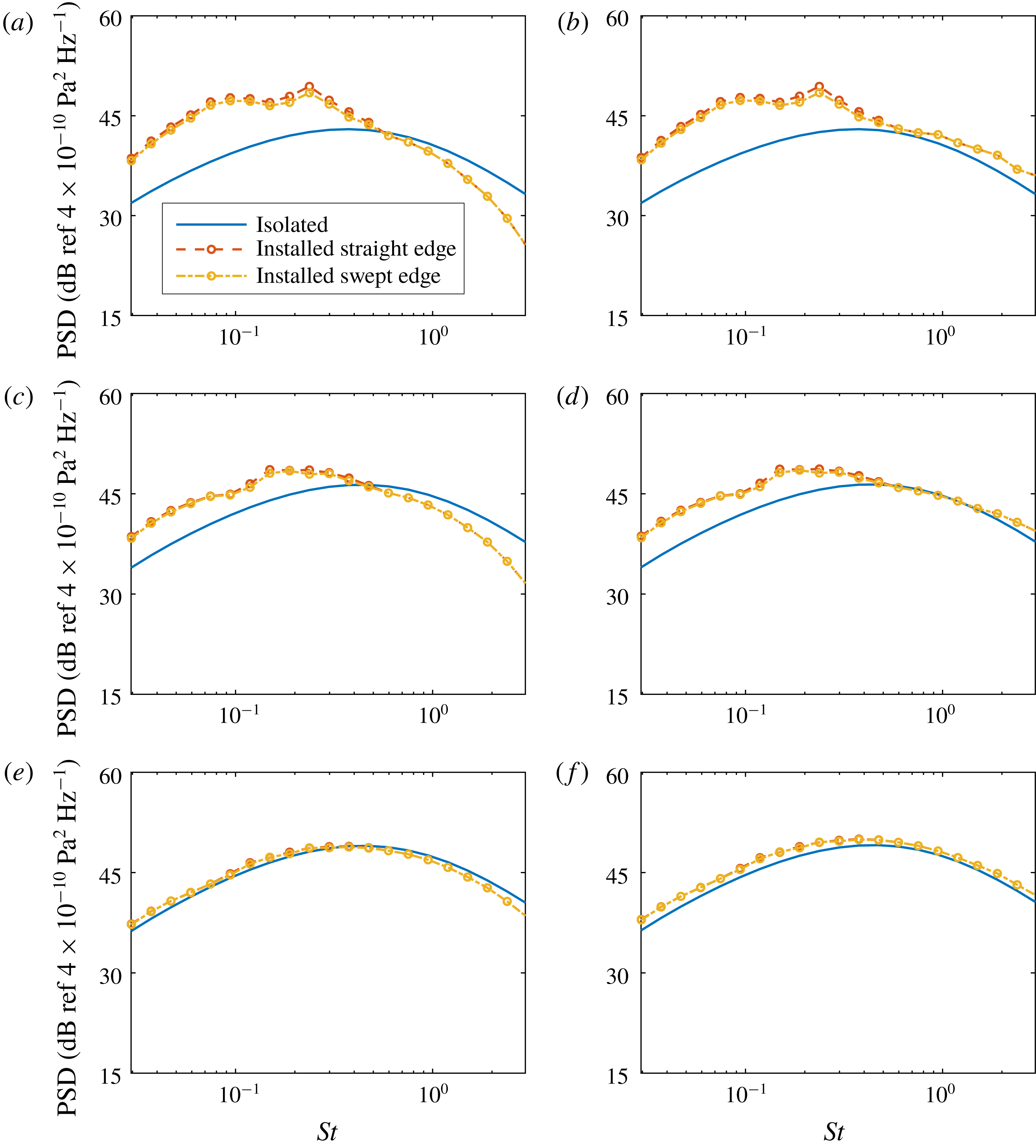
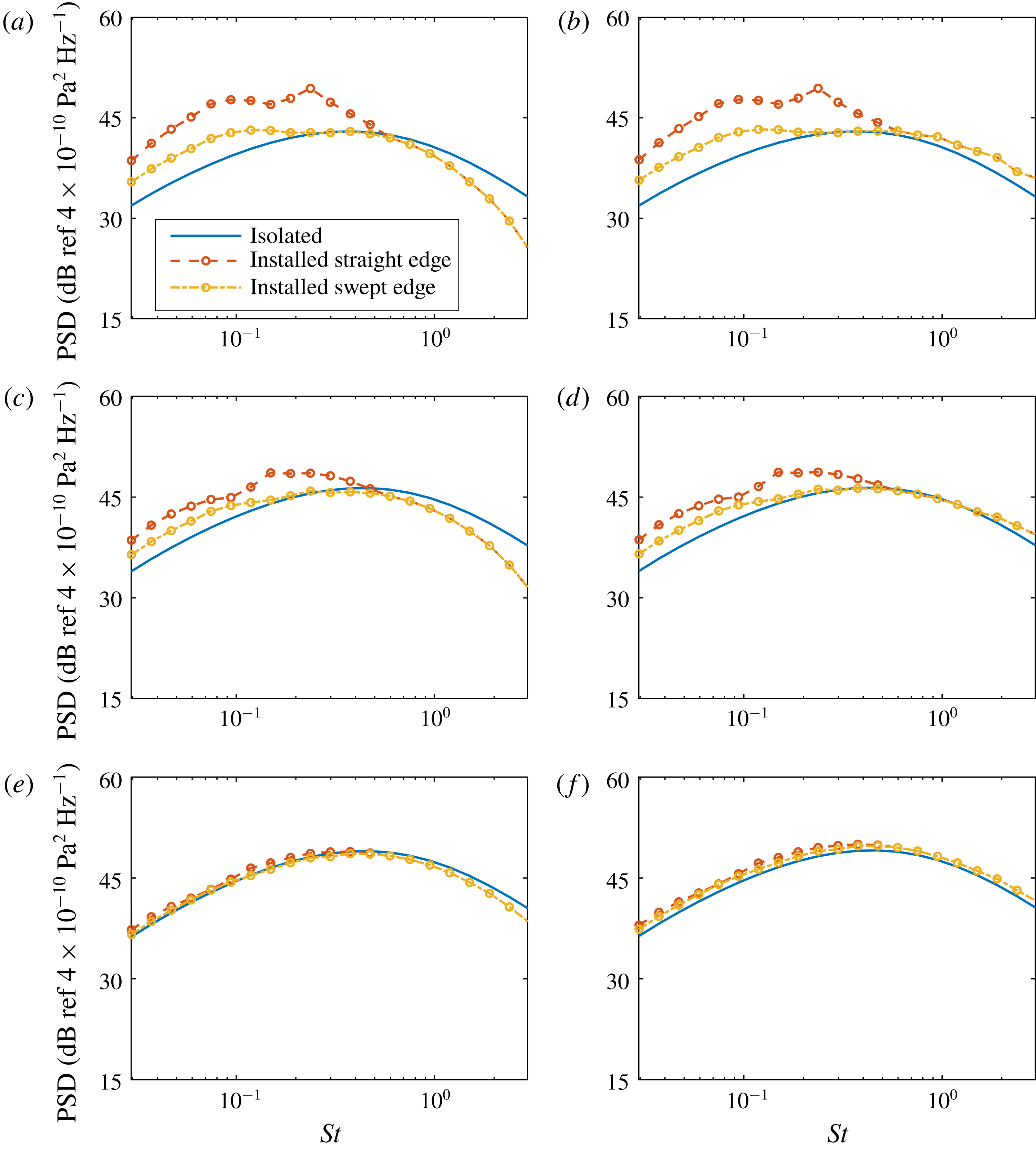
The far-field sound spectra in the mid-span plane at different polar angles for the sweep angle
 $\unicode[STIX]{x1D6FC}=15^{\circ }$
: (a,c,e)
 $90^{\circ }$
,
 $60^{\circ }$
and
 $30^{\circ }$
on the shielded side, respectively; (b,d,f)
 $90^{\circ }$
,
 $60^{\circ }$
and
 $30^{\circ }$
on the reflected side, respectively. The plate is placed at
 $H=1.5D$
and
 $L=4D$
.

Figure 3 shows the far-field sound PSDs at different observer angles for a flat plate with a sweep angle of
 $15^{\circ }$
. The observer is at a distance of
 $50D$
from the centre of the jet nozzle. The plate is placed at
 $H=1.5D$
and
 $L=4D$
. We choose this configuration as a starting point, because the experimental results for this configuration are also available (see § 5). A previous LES study (Lyu et al.
Reference Lyu, Dowling and Naqavi2017) showed that the plate is still outside the jet plume at this position so the characteristics of the instability waves are unlikely to be changed significantly compared to an isolated jet. For reference, the isolated spectra predicted according to the earlier work (Lyu & Dowling Reference Lyu and Dowling2017) are also plotted in the figure. Figure 3(a) shows the spectra when the observer is at
 $90^{\circ }$
on the shielded side of the plate. We can see that the installation effects are significant at low frequencies due to the scattering of instability waves, and a negligible noise reduction is achieved at these frequencies by using swept edges. The results at high frequencies are for reference only since we are primarily interested in low frequencies. Figures 3(c) and 3(e) show the spectra at
 $60^{\circ }$
and
 $30^{\circ }$
on the shielded sides, respectively. It can be seen that the advantages of using swept wings predicted by the model diminish as the observer angle decreases. The trends at low frequencies are similar on the other side of the plate, as demonstrated by figure 3(b,d,f). The prediction that negligible noise reduction is achieved by using a slightly swept edge is consistent with our discussion in the preceding section and the experimental results of Piantanida et al. (Reference Piantanida, Jaunet, Huber, Wolf, Jordan and Cavalieri2016).
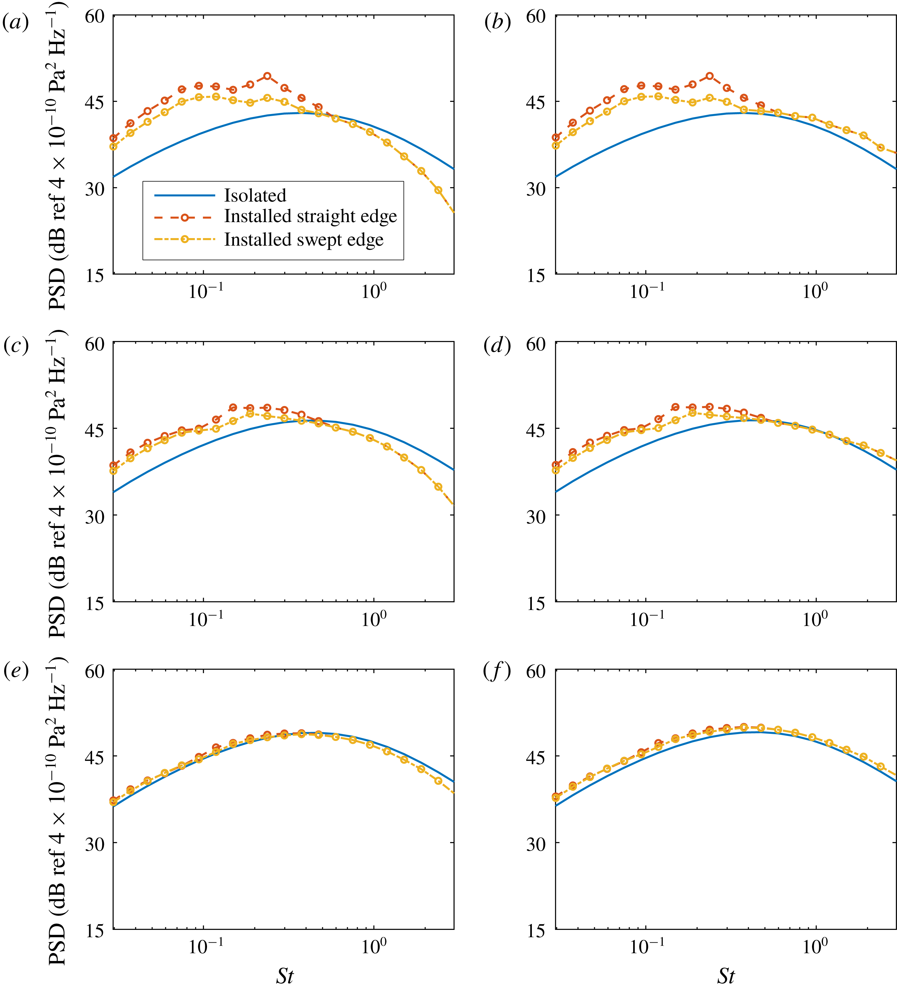
The far-field sound spectra in the mid-span plane at different polar angles for the sweep angle
 $\unicode[STIX]{x1D6FC}=30^{\circ }$
: (a,c,e)
 $90^{\circ }$
,
 $60^{\circ }$
and
 $30^{\circ }$
on the shielded side, respectively; (b,d,f)
 $90^{\circ }$
,
 $60^{\circ }$
and
 $30^{\circ }$
on the reflected side, respectively. The plate is placed at
 $H=1.5D$
and
 $L=4D$
.

The results when the sweep angle is
 $30^{\circ }$
are shown in figure 4. The prediction that a more effective noise reduction can be achieved in this case is clearly verified. Figure 4(a) shows that an average 3 dB noise reduction is achieved at low frequencies when the observer is at
 $90^{\circ }$
above the trailing edge in the mid-span plane. The reduction is still effective at very low frequencies. However, it should be noted that the model assumes that the span is sufficiently long, and this assumption is less likely to be accurate at lower frequencies, where a longer span is required. Hence, in practice, we might see that the noise reduction becomes less effective at lower frequencies. Figure 4(c) shows the results for an observer at
 $60^{\circ }$
. It is clear that the reduction is now much less effective with an average noise reduction of just 1 dB. When the observer is at
 $30^{\circ }$
on the shielded side, the installation effects are negligible, and so is the reduction due to swept edges. The trends are again very similar on the other side of the plate.
The far-field sound spectra in the mid-span plane at different polar angles for the sweep angle
 $\unicode[STIX]{x1D6FC}=45^{\circ }$
: (a,c,e)
 $90^{\circ }$
,
 $60^{\circ }$
and
 $30^{\circ }$
on the shielded side, respectively; (b,d,f)
 $90^{\circ }$
,
 $60^{\circ }$
and
 $30^{\circ }$
on the reflected side, respectively. The plate is placed at
 $H=1.5D$
and
 $L=4D$
.

When the sweep angle is increased to
 $45^{\circ }$
, figure 5(a) shows that a noise reduction of 6–7 dB can be achieved for an observer at
 $90^{\circ }$
. A slight less effective reduction is observed at
 $60^{\circ }$
, while both the installation effects and reduction are negligible at
 $30^{\circ }$
. In summary, we see that in order to achieve an effective noise reduction, the sweep angle should be sufficiently large and this is consistent to our discussion in the preceding section and the experimental results of Piantanida et al. (Reference Piantanida, Jaunet, Huber, Wolf, Jordan and Cavalieri2016). The principal sound-reduction mechanism is destructive interference.
We can also show the azimuthal directivity patterns and how the swept wing changes them. In what follows, the azimuthal (
 $\unicode[STIX]{x1D703}$
) directivity patterns for the fixed polar angle
 $90^{\circ }$
are shown. Again we show the total sound spectra with the straight-edge acoustic-scattering contribution added in for reference. The isolated spectra are also plotted for extra reference.
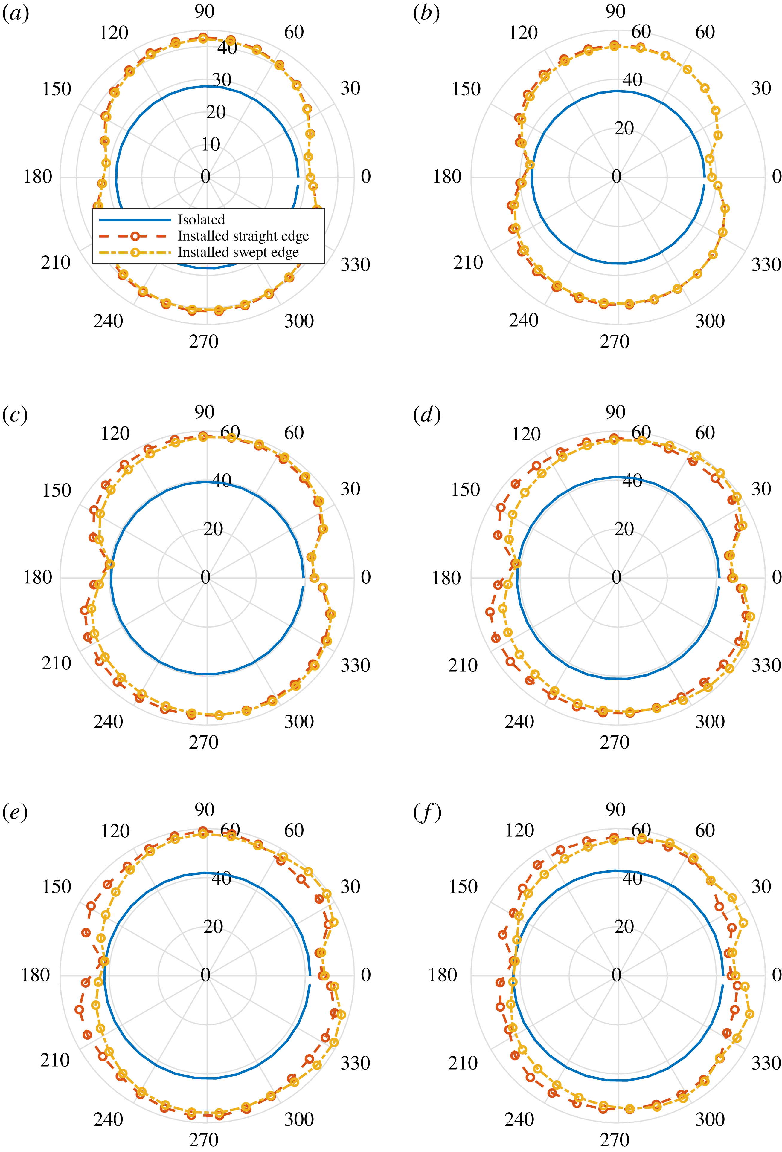
The far-field sound azimuthal directivity (PSD in dB with a reference value
 $4\times 10^{-10}~\text{Pa}^{2}~\text{Hz}^{-1}$
) for the fixed polar angle
 $90^{\circ }$
for the sweep angle
 $\unicode[STIX]{x1D6FC}=15^{\circ }$
: (a)
 $St=0.02$
; (b)
 $St=0.05$
; (c)
 $St=0.1$
; (d)
 $St=0.15$
; (e)
 $St=0.2$
; (f)
 $St=0.3$
. The plate is placed at
 $H=1.5D$
and
 $L=4D$
.

When the sweep angle is
 $15^{\circ }$
, negligible sound reduction can be achieved at
 $St=0.02$
, as shown by figure 6(a). Similar results can be observed for
 $St=0.05$
. A slight noise reduction can be found when
 $St=0.1$
at large azimuthal angles. However, at small azimuthal angles no sound reduction or even a slight noise increase can be observed. This implies that the directivity becomes asymmetric across the mid-span plane. This tendency can be seen more clearly when
 $St$
increases to 0.2, as shown in figure 6(d). At even higher
 $St$
, the asymmetry of the azimuthal directivity becomes even clearer. This change of directivity was observed in the experiment of Piantanida et al. (Reference Piantanida, Jaunet, Huber, Wolf, Jordan and Cavalieri2016) and we will see at a later stage that this is the result of destructive interference.
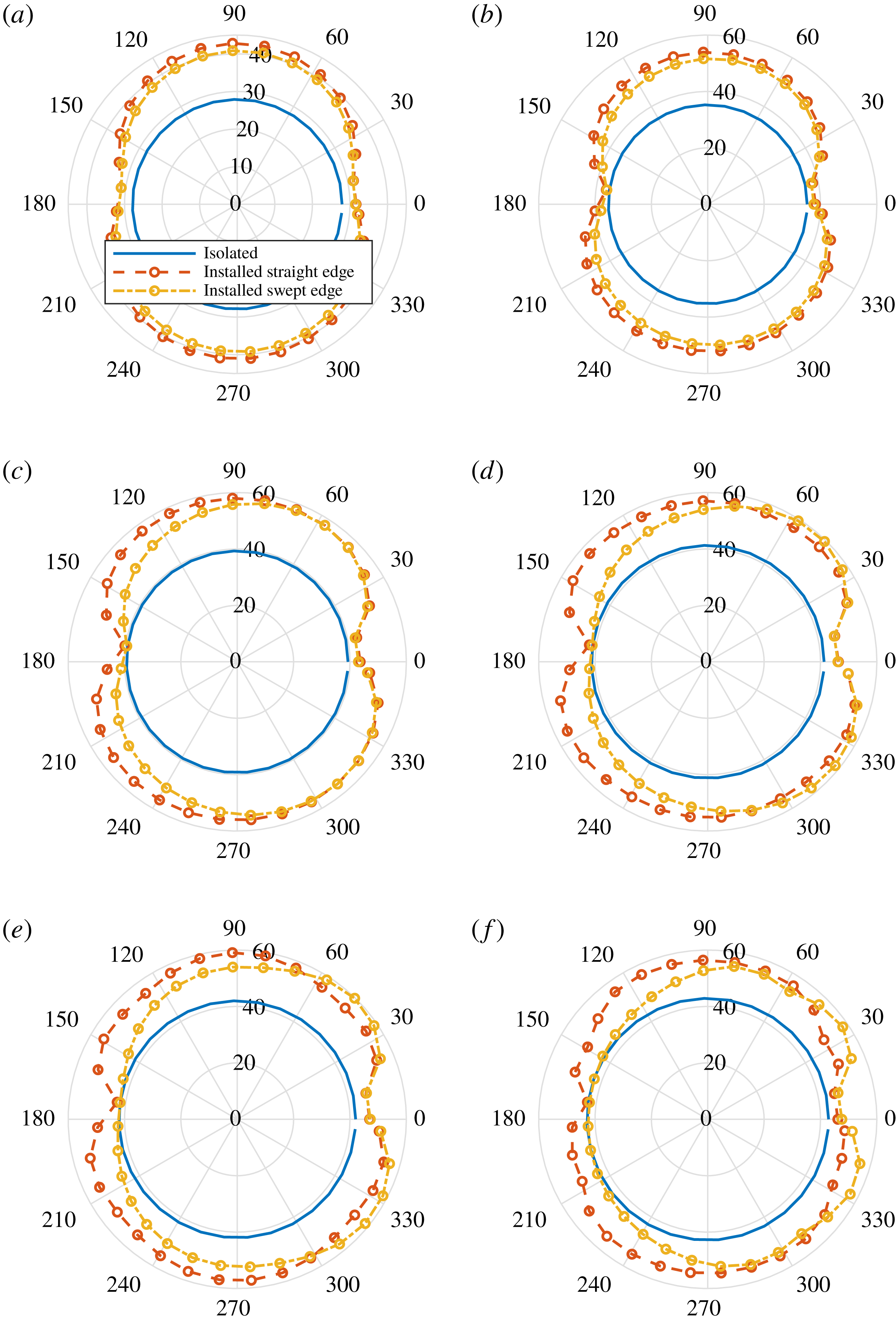
The directivity patterns for the sweep angle
 $\unicode[STIX]{x1D6FC}=30^{\circ }$
are shown in figure 7. Apart from a more effective sound reduction and more evident change of directivity patterns at relatively high frequencies, the results are very similar to those shown in figure 6. One can also expect the same trends when the sweep angle is increased to
 $\unicode[STIX]{x1D6FC}=45^{\circ }$
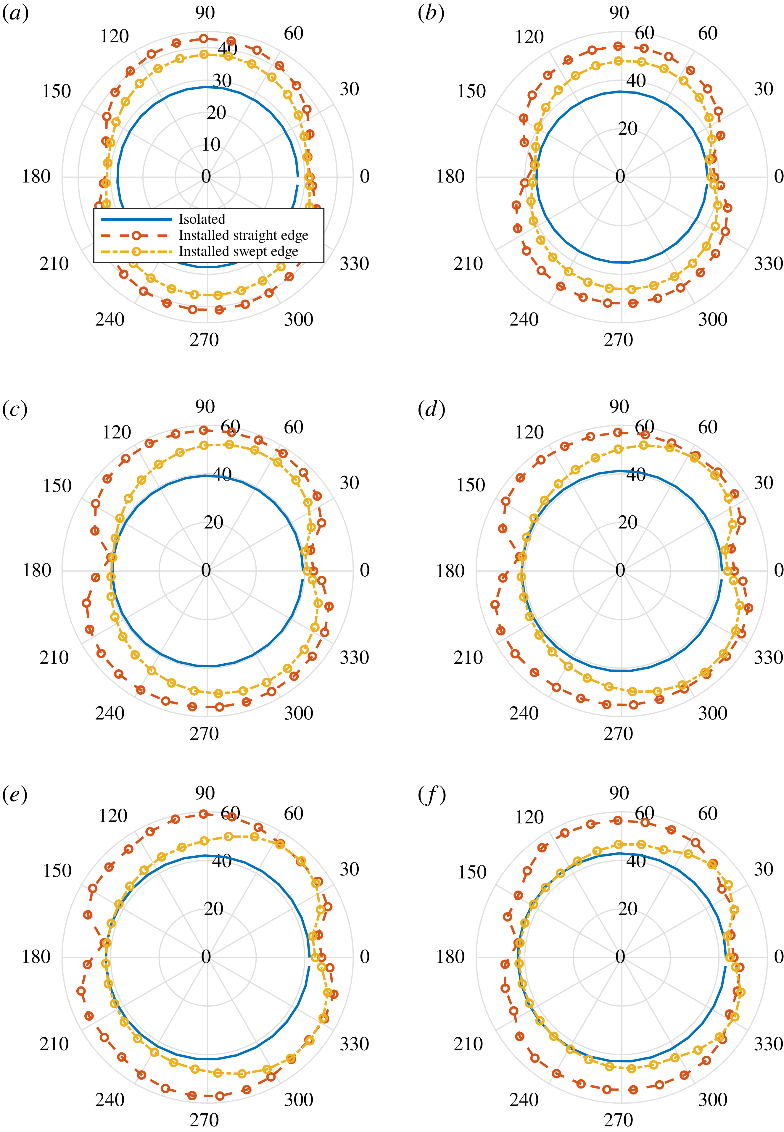
, which is shown in figure 8. However, it is worth noting that in spite of similar changes in the directivity pattern, virtually no sound increase is observed at small azimuthal angles, which is in contrast to the results shown in figures 6 and 7.
The far-field sound azimuthal directivity (PSD in dB with a reference value
 $4\times 10^{-10}~\text{Pa}^{2}~\text{Hz}^{-1}$
) for the fixed polar angle
 $90^{\circ }$
for the sweep angle
 $\unicode[STIX]{x1D6FC}=30^{\circ }$
: (a)
 $St=0.02$
; (b)
 $St=0.05$
; (c)
 $St=0.1$
; (d)
 $St=0.15$
; (e)
 $St=0.2$
; (f)
 $St=0.3$
. The plate is placed at
 $H=1.5D$
and
 $L=4D$
.

The far-field sound azimuthal directivity (PSD in dB with a reference value
 $4\times 10^{-10}\text{ Pa}^{2}~\text{Hz}^{-1}$
) for the fixed polar angle
 $90^{\circ }$
for the sweep angle
 $\unicode[STIX]{x1D6FC}=45^{\circ }$
: (a)
 $St=0.02$
; (b)
 $St=0.05$
; (c)
 $St=0.1$
; (d)
 $St=0.15$
; (e)
 $St=0.2$
; (f)
 $St=0.3$
. The plate is placed at
 $H=1.5D$
and
 $L=4D$
.

The change of directivity pattern is very interesting. We can show that this is a consequence of the destructive interference effect. Recall that
 $$\begin{eqnarray}\displaystyle k_{o}=-k_{1}\unicode[STIX]{x1D70E}+kx_{2}/S_{0}+(k/\unicode[STIX]{x1D6FD}^{2})(x_{1}/S_{0}-M_{a})\unicode[STIX]{x1D70E}, & & \displaystyle\end{eqnarray}$$
which depends on the value of
 $x_{2}$
. From the discussion in § 3, we can see that the sound reduction is due to a sufficiently large non-zero value of
 $|k_{o}|$
. The larger the value is, the more effective reduction we can expect. Therefore, when
 $x_{2}$
is negative, the absolute value of
 $k_{o}$
is larger, hence there is a more effective sound reduction at large azimuthal angles. On the other hand, when
 $x_{2}$
is positive, the value of
 $|k_{o}|$
becomes smaller, resulting in less effective sound reduction. However, when
 $\unicode[STIX]{x1D70E}$
is sufficiently large, we can see that even for
 $x_{2}/S_{0}\rightarrow 1$
the value of
 $|k_{o}|$
is still a sufficiently large non-zero value and hence no noise increase is found, as shown in figure 8.
In figures 3–8, the contribution of the quadrupoles scattered by a straight edge is used instead of that by a swept edge for reference. One might wonder how it differs from the true spectrum when a swept edge is used. We expect the difference to be small, especially for observers in the mid-span plane. This is for two reasons. Firstly, the earlier study by Lyu et al. (Reference Lyu, Dowling and Naqavi2017) found that in the low-frequency regime (e.g.
 $St<0.3$
) the acoustic scattering effect of the quadrupole sources is negligible and their contribution to the far-field sound is virtually identical to that of an isolated jet. Hence one can expect the same is true even if a swept edge is used and there would be little difference between the straight- and swept-edge cases in terms of the sound contribution from quadrupole sources. Secondly, in the high-frequency regime (e.g.
 $St>0.3$
), the contribution from quadrupole sources is dominant and the contribution from instability wave scattering is negligible. But because we now understand that the physical mechanisms of sound alteration in this frequency regime are simply the shielding and reflection effects of the flat plate, we can expect minimal changes to the far-field spectra to occur when we use a swept trailing edge, apart from the fact that both the shielding and reflection effects are slightly more effective on the side where the chord of the flat plate is longer and less effective on the other. Hence, we can see that using spectra for a straight edge for reference is reasonable.
5 Comparison with previous experimental results
The model can now be compared against the experiment carried out by Piantanida et al. (Reference Piantanida, Jaunet, Huber, Wolf, Jordan and Cavalieri2016). In the experiment, the jet diameter
 $D$
was 0.05 m and the jet Mach number was 0.4. Four flat plates were used, and their trailing edges were tilted by
 $0^{\circ }$
,
 $15^{\circ }$
,
 $30^{\circ }$
and
 $45^{\circ }$
, respectively. All these plates shared the same average chord
 $c=9D$
and span
 $d=15D$
. During the experiment, these plates were placed near the jet at
 $H=1.5D$
and
 $L=4D$
and the jet centreline was aligned with the middle span of these plates. The azimuthal directivity at
 $St=0.2$
was measured at a distance of
 $14.3D$
from the jet centreline, at the axial location
 $x_{1}=0$
.
To compare our model with experimental results, the contribution from the Lighthill quadrupole sources is first obtained according to the results shown in the earlier work by Lyu et al. (Reference Lyu, Dowling and Naqavi2017). The validity of doing so has been discussed in § 4. In fact, the scattering of the quadrupole sources by a semi-infinite flat plate with a swept trailing edge can be modelled analytically. But having recognized that it is virtually the same as that for the straight edge in the frequency range of interest, and that the primary purpose of this paper is to model the noise due to the scattering of jet instability waves, such an endeavour seems to be unnecessary. Secondly, the contribution due to the scattering of the near-field instability waves is obtained from (2.25). The near-field spectrum at only
 $St=0.2$
(one point on the full spectrum) is needed. Because we do not yet have an experimental database for such a spectrum for a jet of Mach number 0.4, the amplitude of such a spectrum at
 $St=0.2$
is chosen such that the far-field sound for the straight edge matches the corresponding experimental results. This amplitude is subsequently used to predict the results for swept edges.
Comparison of the azimuthal noise directivity (PSD in dB with a reference value
 $4\times 10^{-10}~\text{Pa}^{2}~\text{Hz}^{-1}$
) for a fixed polar angle of
 $90^{\circ }$
between the model and experiment when
 $\unicode[STIX]{x1D6FC}=15^{\circ }$
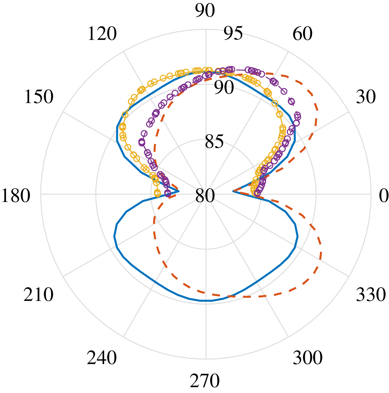
; blue solid: prediction for straight edge; red dashed: prediction for swept edge; yellow solid with markers: measurement for straight edge; purple dashed with markers: prediction for swept edge.

Results when the trailing edge is tilted by
 $15^{\circ }$
are shown in figure 9. The experimental results are shown only on the shielded side of the plate. This is because the scattered sound on this side is not affected by the refraction effect of the jet plume. As we can see from the figure, the predicted directivity shape for the straight edge agrees well with the experimental result. When the straight edge is replaced with a swept edge, the experiment reveals that a noticeable noise reduction can be achieved. In particular, greater reduction occurs at large azimuthal angles (close to
 $180^{\circ }$
). At low azimuthal angles (close to
 $0^{\circ }$
), a slight noise increase occurs. This difference in the noise reduction effectively changes the directivity pattern from a symmetric to titled shape. Such a change is well captured by the model, especially at large azimuthal angles. The slight disagreement at low azimuthal angles, however, could be caused by the side edges of the plates and/or the slow variation of jet instability spectra along the axial direction (because the trailing edge is swept, so strictly speaking the scattering occurs locally at different axial locations, but the slow spectra variation because of this is ignored in the model).
Comparison of the azimuthal noise directivity (PSD in dB with a reference value
 $4\times 10^{-10}~\text{Pa}^{2}~\text{Hz}^{-1}$
) for a fixed polar angle of
 $90^{\circ }$
between the model and experiment when
 $\unicode[STIX]{x1D6FC}=30^{\circ }$
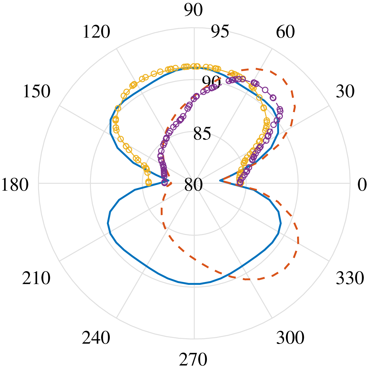
; blue solid: prediction for straight edge; red dashed: prediction for swept edge; yellow solid with markers: measurement for straight edge; purple dashed with markers: prediction for swept edge.

When the sweep angle increases to
 $30^{\circ }$
, as shown in figure 10, the experimental noise reduction is more pronounced. The change to the directivity from a symmetric to tilted pattern remains the same, and at low azimuthal angles a slight noise increase still occurs. The model predicts both behaviours very well. In particular, the predicted noise spectrum in the large azimuthal angle range has a nearly perfect agreement with the experimental result. The agreement at low azimuthal angles is not quite as good as that at high angles, and this might have been for the same reasons as described in the preceding paragraph.
Comparison of the azimuthal noise directivity (PSD in dB with a reference value
 $4\times 10^{-10}~\text{Pa}^{2}~\text{Hz}^{-1}$
) for a fixed polar angle of
 $90^{\circ }$
between the model and experiment when
 $\unicode[STIX]{x1D6FC}=45^{\circ }$
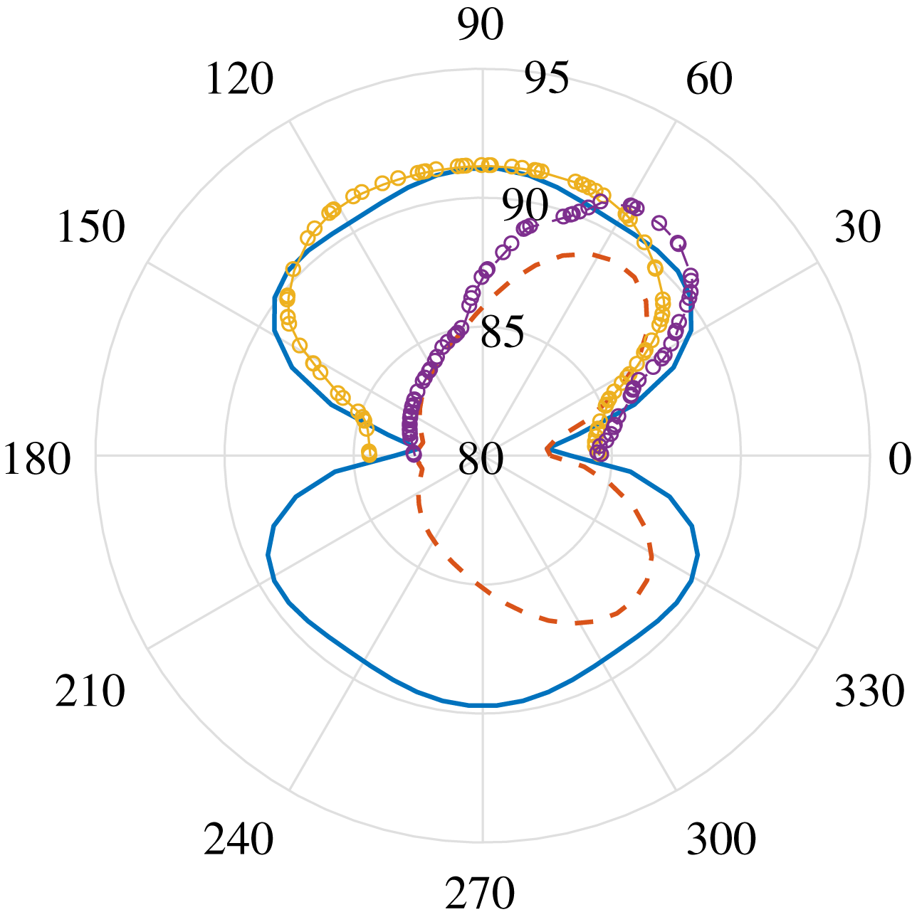
; blue solid: prediction for straight edge; red dashed: prediction for swept edge; yellow solid with markers: measurement for straight edge; purple dashed with markers: prediction for swept edge.

Figure 11 shows the comparison for the largest sweep angle, i.e.
 $45^{\circ }$
. The maximum noise reduction, up to 8 dB, occurs at around the azimuthal angle
 $130^{\circ }$
. The agreement between the experimental results and the model predictions continues to be good. We note again that deviation occurs mostly at low azimuthal angles, with possible causes discussed above. The good agreement shown in this section suggests that the current model can capture the scattering physics very well, and also demonstrates that the destructive interference is the main mechanism of sound reduction by using aircraft wings with swept trailing edges.
6 Conclusion
This paper develops an analytical model to predict the noise due to the scattering of instability waves by an aircraft wing with a swept trailing edge. The aircraft wing is simplified as a flat plate and a uniform ambient mean flow is assumed. The Schwarzchild method is used to obtain the scattered pressure on the surface while the far-field sound is obtained via a surface pressure integral.
The model can correctly predict both the magnitude of the sound reduction and the changes to the directivity patterns. Very good agreement is achieved between the developed model and a previous experiment. It is found that the principal mechanism of the sound reduction is due to the destructive interference effect. It is concluded that in order to obtain an effective sound reduction, both the span and the sweep angle of the aircraft wing have to be large. Such a model can serve as a robust tool in quickly evaluating the effects of swept trailing edges on the low-frequency installed jet noise at various design stages. The newly discovered interference mechanism for noise reduction can also provide significant insight into developing other innovative noise-reduction strategies.