1 Introduction
By definition, a complex analytic quasi-ordinary (q.o.) singularity  $(X,0)$ of dimension
 $d$ comes with a finite projection
 $p:X\longrightarrow \mathbb{A}^{d},$ whose discriminant is a normal crossing divisor. These singularities appear in the Jungian approach to resolution of singularities (see [Reference Popescu-Pampu31]). We are interested in irreducible q.o. surfaces
 $X$, defined by
 $f\,\in \,\mathbb{C}\{x_{1},x_{2}\}[z].$ Thanks to the Abhyankar–Jung theorem, we know that a hypersurface of this type is parametrized in the form
 $x_{i}=x_{i}$ for
 $i=1,2$ and
 $z=\unicode[STIX]{x1D701}(x_{1},x_{2})$, where
 $\unicode[STIX]{x1D701}$ is an element in
 $\mathbb{C}\{x_{1}^{1/n},x_{2}^{1/n}\},n$ being the degree of
 $f$ as a polynomial in
 $z.$ Moreover, some special exponents (called the characteristic exponents) which belong to the support of the series
 $\unicode[STIX]{x1D701}$, are complete invariants of the topological type of the singularity (see [Reference Gau15]). In particular, they determine invariants which come from resolution of singularities, like the log-canonical threshold or the Motivic zeta functions [Reference Artal Bartolo, Cassou-Noguès, Luengo and Melle Hernández3, Reference Budur, González Pérez and González Villa8, Reference Cobo Pablos and González Pérez9, Reference González Pérez and González Villa18]. They also give insights about the construction of a resolution of singularities [Reference Ban and McEwan6, Reference Ban and McEwan7, Reference González Pérez17, Reference Villamayor34].
Our aim is to construct some comparable complete invariants for all types of singularities. Since in general, we cannot have a parametrization, we search for such invariants in the jet schemes. For  $m\,\in \,\mathbb{N},$ the
 $m$th jet scheme, denoted by
 $X_{m}$, is a scheme that parametrizes morphisms
 $\text{Spec }\mathbb{C}[t]/(t^{m+1})\longrightarrow X.$ Intuitively we can think of it as a scheme parametrizing arcs in an ambient space, which have contact at least
 $m+1$ with
 $X.$ We know already that some invariants which come from resolution of singularities are encoded in the jet schemes [Reference Ein and Mustaţa13, Reference Mustaţa29].
We want to extract from the jet schemes information about the singularity, which can be expressed in terms of invariants of resolutions of singularities. For specific types of singularities, the knowledge of the irreducible components of the jet schemes  $X_{m}$ of a singular variety
 $X$, together with some of their invariants, such as dimension or embedding dimension, allows us to determine deep invariants of the singularity of
 $X$: the topological type in the case of curves (see [Reference Mourtada24]), and the analytical type in the case of normal toric surfaces (see [Reference Mourtada25]). Moreover, in the case of irreducible plane curves, the minimal embedded resolution can be constructed from the jet schemes [Reference Lejeune-Jalabert, Mourtada and Reguera21], and the same holds for rational double point singularities [Reference Mourtada and Plénat28].
Understanding the structure of jet schemes for particular singularities is an interesting problem. It has been studied in [Reference Yuen35] and [Reference Docampo12] for determinantal varieties, in [Reference Mourtada24] for plane curve singularities, in [Reference Mourtada25] for normal toric surfaces, in [Reference Mourtada26] for rational double point surface singularities, and in [Reference Sethuraman and Šivic33] for commuting matrix pairs schemes.
In this paper, we study jet schemes of a two-dimensional, irreducible q.o. hypersurface singularity  $X=\{f=0\}$, with
 $f\,\in \,\mathbb{C}\{x_{1},x_{2}\}[z]$. We give a combinatorial description of the irreducible components of the set of
 $m$-jets with center in the singular locus of
 $X$, in terms of invariants of the singularity extracted from the characteristic exponents of
 $X$. We define the candidates to be the irreducible components
 $C_{m}^{\unicode[STIX]{x1D708}}$, but there are many inclusions among these candidates. We study these inclusions by defining on
 $\mathbb{Z}_{{\geqslant}0}^{2}$ a subtle relation depending on
 $m$ and expressed in terms of the invariants cited above. It reflects the evolution of the singular loci of q.o. surfaces approximating our surface
 $X$.
Then, with the minimal elements with respect to this relation we define a set  $F_{m}\subset \mathbb{Z}^{2}$, and for any
 $\unicode[STIX]{x1D708}\,\in \,F_{m}$, we have a component
 $C_{m}^{\unicode[STIX]{x1D708}}\subset X_{m}$. We prove that these are the irreducible components of
 $m$-jets through the singular locus.
Theorem 1.1. Let  $X$ be a q.o. hypersurface of dimension two. For any
 $m\,\in \,\mathbb{Z}_{{>}0},$ the scheme of
 $m$th jet of
 $X$ with center in its singular locus has the following decomposition into irreducible components
 $$\begin{eqnarray}\big(\unicode[STIX]{x1D70B}_{m}^{-1}(X_{\text{Sing}})\big)_{\text{red}}=\mathop{\bigcup }_{\unicode[STIX]{x1D708}\in F_{m}}C_{m}^{\unicode[STIX]{x1D708}},\end{eqnarray}$$
where  $\unicode[STIX]{x1D70B}_{m}:X_{m}\longrightarrow X$ is induced by projection.
Note that if we choose an affine variety  $Y\subset \mathbb{C}^{3}$ which has a q.o. singularity at a point
 $x,$ then after shrinking
 $Y$ into a small enough neighborhood of
 $x,$ this gives us the decomposition of
 $Y_{m}$ into irreducible components, modulo adding the component obtained as the Zariski closure of the set of jets whose center is in the regular locus of
 $Y.$
In general, for any algebraic variety  $V,$ the irreducible components of the jet schemes
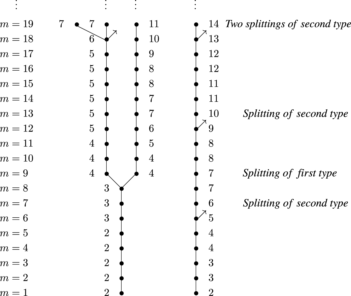
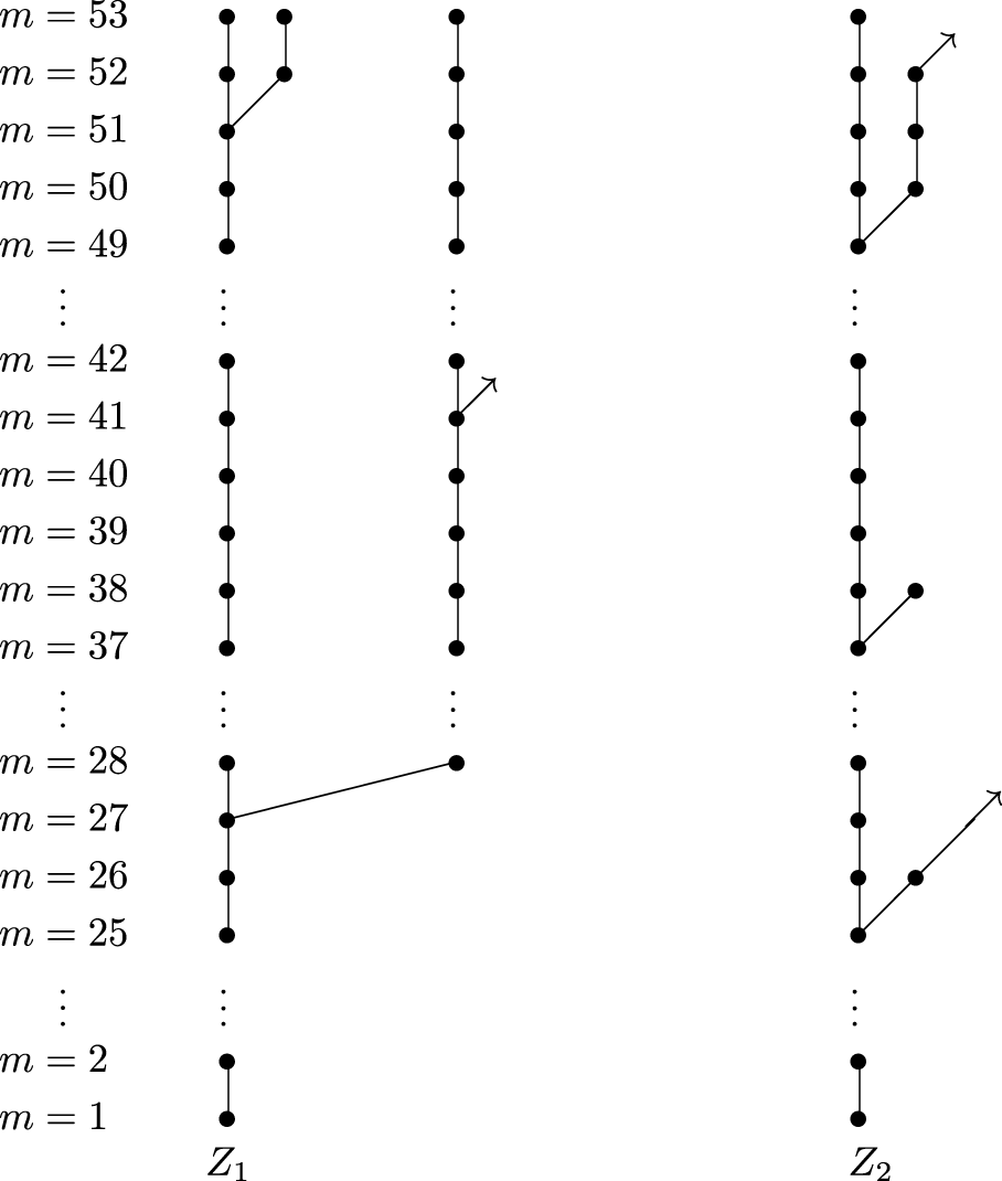
 $V_{m}$ fit in natural projective systems, to which we associate a weighted graph. Graphs are a powerful tool for studying surface singularities (see [Reference Popescu-Pampu32] for a nice and historical introduction on this topic). The vertices of our graph correspond to irreducible components, and to every vertex we attach the corresponding embedding dimension and codimension in the jet scheme of the ambient space. We will prove the following result.
Theorem 1.2. Let  $X$ be a q.o. hypersurface of dimension two. The weighted graph associated with the irreducible components of jets through the singular locus determines and it is determined by the topological type of the singularity.
This theorem achieves one of our goals for this type of singularities: constructing a complete invariant of the topological type of the singularity from its jet schemes; while the graph of the jet schemes is defined in general, the characteristic exponents, which are also a complete invariant of q.o. singularities, does not have a meaning for more general singularities for two reasons: (1) for a general singularity we only have parametrizations of parts of the singularity (wedges), (2) the shape of these parametrizations is more complicated than the shape of parametrizations of q.o. singularities.
It is also important to stress that other invariants involving arcs and jets, like motivic zeta functions, do not determine the topological type in the case of q.o. singularities; see [Reference Cobo Pablos and González Pérez9] and [Reference González Pérez and González Villa18].
We devote Section 4 to study in detail the case of q.o. surfaces with only one characteristic exponent, and in the next section we deal with the general case.
In another direction, using Mustaţa’s formula [Reference Mustaţa29], we determine an irreducible component of an  $m$th jet scheme, or equivalently a divisorial valuation on the ambient space
 $\mathbb{A}^{3}$, which computes the log-canonical threshold of the pair
 $X\subset \mathbb{A}^{3}$ (the log-canonical threshold for such a pair has been computed in [Reference Budur, González Pérez and González Villa8], looking at the poles of the motivic zeta function). This provides us with pairs
 $X\subseteq \mathbb{A}^{3}$ whose log-canonical threshold is not computed by a monomial divisorial valuation. The q.o. surface in
 $\mathbb{A}^{3}$ defined by
 $f=(z^{2}-x_{1}x_{2})^{2}-x_{1}^{3}x_{2}z$ is such a pair. Note that for a pair
 $C\subseteq \mathbb{A}^{2}$, where
 $C$ is a plane curve, the log-canonical threshold is always computed by a monomial valuation. See [Reference Artal Bartolo, Cassou-Noguès, Luengo and Melle-Hernández4] and [Reference Aprodu and Naie2] for the computation of the log-canonical threshold for plane curves.
Using same ideas of [Reference Mourtada27], it seems possible to construct an embedded resolution of singularities of  $X$ from the data of the graph constructed in this paper. We think that such a resolution would shed light on the resolution of singularities obtained by González Pérez in [Reference González Pérez17], and would make more precise his answer to the question of Lipman (see [Reference Lipman23]) on the construction of a canonical resolution of singularities of a q.o. hypersurface from its characteristic exponents.
2 Jet schemes
In this section we define jet schemes of an affine scheme  $X;$ see [Reference Ein and Mustaţa13] and [Reference Ishii19] for details. Let
 $X=\text{Spec}\,\mathbb{C}[x_{1},\ldots ,x_{n}]/I$ be an affine scheme of finite type. For
 $m\,\in \,\mathbb{Z}_{{>}0}$ the functor
 $F_{m}:~\mathbb{C}\text{-Schemes}\longrightarrow \text{Sets}$ which, with an affine scheme defined by a
 $\mathbb{C}$-algebra
 $A$, associates
 $$\begin{eqnarray}F_{m}\big(\text{Spec}(A)\big)=\text{Hom}_{\mathbb{C}}\big(\text{Spec}(A[t]/(t^{m+1})),X\big),\end{eqnarray}$$
is representable by a  $\mathbb{C}$-scheme, denoted by
 $X_{m}$. This is the scheme of
 $m$-jets. Its closed points are morphisms of the form
 $$\begin{eqnarray}\unicode[STIX]{x1D6FE}:\text{Spec}(\mathbb{C}[t]/(t^{m+1}))\longrightarrow X.\end{eqnarray}$$
Such a morphism  $\unicode[STIX]{x1D6FE}$ is equivalent to a
 $\mathbb{C}$-algebra homomorphism
 $$\begin{eqnarray}\unicode[STIX]{x1D6FE}^{\ast }:\mathbb{C}[x_{1},\ldots ,x_{n}]/I\longrightarrow \mathbb{C}[t]/(t^{m+1}).\end{eqnarray}$$
If we fix a set of generators  $f_{1},\ldots ,f_{r}$ for the ideal
 $I$, the map
 $\unicode[STIX]{x1D6FE}^{\ast }$ is determined by the image of the
 $x_{i}$
 $$\begin{eqnarray}x_{i}\mapsto x_{i}^{(0)}+x_{i}^{(1)}t+\cdots +x_{i}^{(m)}t^{m},\quad 1\leqslant i\leqslant n,\end{eqnarray}$$
where the relations
 $$\begin{eqnarray}\displaystyle f_{i}\big(x_{1}^{(0)}+\cdots +x_{1}^{(m)}t^{m},\ldots ,x_{n}^{(0)}+\cdots +x_{n}^{(m)}t^{m}\big)\equiv 0~\text{mod}~t^{m+1} & & \displaystyle\end{eqnarray}$$
must hold for each  $f_{i}$, with
 $1\leqslant i\leqslant r$. If we write
 $$\begin{eqnarray}\displaystyle & & \displaystyle f_{i}\big(x_{1}^{(0)}+x_{1}^{(1)}t+\cdots +x_{1}^{(m)}t^{m},\ldots ,x_{n}^{(0)}+x_{n}^{(1)}t+\cdots +x_{n}^{(m)}t^{m}\big)\nonumber\\ \displaystyle & & \displaystyle \quad =\mathop{\sum }_{j=0}^{m}F_{i}^{(j)}(x_{1}^{(0)},\ldots ,x_{1}^{(j)},\ldots ,x_{n}^{(0)},\ldots ,x_{n}^{(j)})~t^{j}~\text{mod}~t^{m+1},\end{eqnarray}$$
we have that giving a closed point of  $X_{m}$ is equivalent to giving a point in
 $$\begin{eqnarray}V(F_{l}^{(j)})_{0\leqslant j\leqslant m,1\leqslant l\leqslant r}\subset \mathbb{A}_{m}^{n},\end{eqnarray}$$
where  $\mathbb{A}_{m}^{n}=\text{Spec}(\mathbb{C}[x_{i}^{(0)},\ldots ,x_{i}^{(m)}]_{i=1,\ldots ,n})$. Hence we can make the following identification
 $$\begin{eqnarray}\displaystyle X_{m}=\text{Spec}\left(\frac{\mathbb{C}[x_{i}^{(0)},\ldots ,x_{i}^{(m)}]_{i=1,\ldots ,n}}{\big(F_{l}^{(j)}\big)_{0\leqslant j\leqslant m,1\leqslant l\leqslant r}}\right). & & \displaystyle\end{eqnarray}$$
We can give a useful relation among the  $F_{l}^{(j)}$ in terms of derivations. Let
 $\unicode[STIX]{x1D6FF}$ be the
 $\mathbb{C}$-derivation on
 $\mathbb{C}[x_{i}^{(0)},\ldots ,x_{i}^{(m)}]_{i=1,\ldots ,n}$ defined by
 $$\begin{eqnarray}\unicode[STIX]{x1D6FF}(x_{i}^{(m)})=0\qquad \text{and}\qquad \unicode[STIX]{x1D6FF}(x_{i}^{(j)})=x_{i}^{(j+1)}\quad \text{for }0\leqslant j<m.\end{eqnarray}$$
For  $f\,\in \,\mathbb{C}[x_{1},\ldots ,x_{n}]$ let
 $f^{(0)}=f(x_{1}^{(0)},\ldots ,x_{n}^{(0)})$,
 $f^{(1)}:=\unicode[STIX]{x1D6FF}(f)$ and recursively
 $f^{(m)}=\unicode[STIX]{x1D6FF}(f^{(m-1)})$. By using the change of variables
 $$\begin{eqnarray}\begin{array}{@{}ccc@{}}\unicode[STIX]{x1D719}:~\mathbb{C}[x_{i}^{(0)},\ldots ,x_{i}^{(m)}]_{1\leqslant i\leqslant n} & \longrightarrow & \mathbb{C}[x_{i}^{(0)},\ldots ,x_{i}^{(m)}]_{1\leqslant i\leqslant n}\\ x_{i}^{(r)} & \longmapsto & r!x_{i}^{(r)}\end{array}\end{eqnarray}$$
we can prove that
 $$\begin{eqnarray}\unicode[STIX]{x1D719}(f^{(r)})=r!F^{(r)}.\end{eqnarray}$$
Hence we have the following description of the jet schemes, equivalent to (3), coming from differential algebra.
Proposition 2.1. (See [Reference Mourtada24, Proposition 2.3])
Let
 $$\begin{eqnarray}X=\text{Spec}\left(\frac{\mathbb{C}[x_{1},\ldots ,x_{n}]}{(f_{1},\ldots ,f_{r})}\right)\end{eqnarray}$$
and  $m\,\in \,\mathbb{Z}_{{>}0}$, then
 $$\begin{eqnarray}X_{m}=\text{Spec}\left(\frac{\mathbb{C}[x_{i}^{(0)},\ldots ,x_{i}^{(m)}]_{i=1,\ldots ,n}}{\big(f_{i}^{(j)}\big)_{1\leqslant i\leqslant r,0\leqslant j\leqslant m}}\right).\end{eqnarray}$$
Corollary 2.2. Every polynomial  $F^{(l)}$ is nonzero and quasi-homogeneous of degree
 $l$ in
 $x_{k}^{(0)},\ldots ,x_{k}^{(l)}$, for
 $1\leqslant k\leqslant n$. In
 $F^{(0)},\ldots ,F^{(l)}$ the variables
 $x_{k}^{(l)}$ for
 $1\leqslant k\leqslant n$ appear only in
 $F^{(l)}$, and with exponent one.
Example 2.3. Let  $X$ be the q.o. surface defined by the polynomial
 $f=z^{3}-x_{1}^{3}x_{2}^{2}$. The equations defining the
 $3$-jets are (in both descriptions):
 $$\begin{eqnarray}\displaystyle F^{(0)} & = & \displaystyle {z^{(0)}}^{3}-{x_{1}^{(0)}}^{3}{x_{2}^{(0)}}^{2}=f^{(0)}\nonumber\\ \displaystyle F^{(1)} & = & \displaystyle 3{z^{(0)}}^{2}z^{(1)}-3{x_{1}^{(0)}}^{2}x_{1}^{(1)}{x_{2}^{(0)}}^{2}-2{x_{1}^{(0)}}^{3}x_{2}^{(0)}x_{2}^{(1)}=f^{(1)}\nonumber\\ \displaystyle F^{(2)} & = & \displaystyle 3{z^{(0)}}^{2}z^{(2)}+3z^{(0)}{z^{(1)}}^{2}-6{x_{1}^{(0)}}^{2}x_{1}^{(1)}x_{2}^{(0)}x_{2}^{(1)}-2{x_{1}^{(0)}}^{3}x_{2}^{(0)}x_{2}^{(2)}\nonumber\\ \displaystyle & & \displaystyle -\,3{x_{1}^{(0)}}^{2}x_{1}^{(2)}{x_{2}^{(0)}}^{2}-{x_{1}^{(0)}}^{3}{x_{2}^{(1)}}^{2}-3x_{1}^{(0)}{x_{1}^{(1)}}^{2}{x_{2}^{(0)}}^{2}\nonumber\\ \displaystyle & = & \displaystyle {\textstyle \frac{1}{2}}\unicode[STIX]{x1D719}(f^{(2)})={\textstyle \frac{1}{2}}\unicode[STIX]{x1D719}(\unicode[STIX]{x1D6FF}(f^{(1)}))\nonumber\\ \displaystyle F^{(3)} & = & \displaystyle {z^{(1)}}^{3}+6z^{(0)}z^{(1)}z^{(2)}+3{z^{(0)}}^{2}z^{(3)}-2{x_{1}^{(0)}}^{3}x_{2}^{(0)}x_{2}^{(3)}-2{x_{1}^{(0)}}^{3}x_{2}^{(1)}x_{2}^{(2)}\nonumber\\ \displaystyle & & \displaystyle -\,6{x_{1}^{(0)}}^{2}x_{1}^{(1)}x_{2}^{(0)}x_{2}^{(2)}-3{x_{1}^{(0)}}^{2}x_{1}^{(1)}{x_{2}^{(1)}}^{2}-6{x_{1}^{(0)}}^{2}x_{1}^{(2)}x_{2}^{(0)}x_{2}^{(1)}\nonumber\\ \displaystyle & & \displaystyle -\,6x_{1}^{(0)}{x_{1}^{(1)}}^{2}x_{2}^{(0)}x_{2}^{(1)}-3{x_{1}^{(0)}}^{2}x_{1}^{(3)}{x_{2}^{(0)}}^{2}-6x_{1}^{(0)}x_{1}^{(1)}x_{1}^{(2)}{x_{2}^{(0)}}^{2}-{x_{1}^{(1)}}^{3}{x_{2}^{(0)}}^{2}\nonumber\\ \displaystyle & = & \displaystyle \frac{1}{3!}\unicode[STIX]{x1D719}(f^{(3)})=\frac{1}{3!}\unicode[STIX]{x1D719}(\unicode[STIX]{x1D6FF}^{2}(f^{(1)})).\nonumber\end{eqnarray}$$
For  $m>n\geqslant 0$, we have a canonical projection
 $\unicode[STIX]{x1D70B}_{m,n}:X_{m}\longrightarrow X_{n}$ induced by the projection
 $\mathbb{C}[t]/t^{m+1}\longrightarrow \mathbb{C}[t]/t^{n+1}$, and we denote
 $\unicode[STIX]{x1D70B}_{m,0}$ simply by
 $\unicode[STIX]{x1D70B}_{m}:X_{m}\longrightarrow X$.
Proposition 2.4. (see [Reference Denef and Loeser11] and [Reference Ein and Mustaţa13])
If  $X$ is a nonsingular variety of dimension
 $d$ then for any
 $m\geqslant 0$ the projections
 $\unicode[STIX]{x1D70B}_{m+1,m}:X_{m+1}\longrightarrow X_{m}$ are locally trivial with fiber
 $\mathbb{A}^{d}$. In particular
 $X_{m}$ is a nonsingular variety of dimension
 $(m+1)d$.
The above construction of jet schemes in the algebraic case can be done analogously in the analytic case. Indeed, as we will see in the next section, we will deal with  $f\,\in \,\mathbb{C}\{x_{1},x_{2}\}[z]$. Then, for
 $l\,\in \,\mathbb{Z}_{{\geqslant}0}$, denoting by
 $$\begin{eqnarray}R^{(l)}:=\mathbb{C}\{x_{1}^{(0)},x_{2}^{(0)}\}[x_{k}^{(1)},\ldots ,x_{k}^{(l)},z^{(0)},\ldots ,z^{(l)}]_{k=1,2},\end{eqnarray}$$
we have that  $F^{(l)}\,\in \,R^{(l)}$, and
 $$\begin{eqnarray}X_{m}=\text{Spec}\left(\frac{R^{(m)}}{\big(F^{(0)},\ldots ,F^{(m)}\big)}\right).\end{eqnarray}$$
We will anyway speak of the polynomials  $F^{(l)}$ defining the space of
 $m$-jets.
Remark 2.5. To describe the components of  $(\unicode[STIX]{x1D70B}_{m}^{-1}(X_{\text{Sing}}))_{\text{red}}$, since the level
 $m$ is clear from the context, we will use the notation
 $V(I)$ instead of the more accurate one Spec
 $(R^{(m)}/I)$.
3 Quasi-ordinary surface singularities
In this section we collect some well known facts about q.o. hypersurface singularities of dimension two. We state everything for the case of surfaces, though the definitions and results hold in any dimension.
An equidimensional germ  $(X,0)$, of dimension two, is quasi-ordinary (q.o. for short) if there exists a finite projection
 $p:(X,0)\rightarrow (\mathbb{C}^{2},0)$ which is a local isomorphism outside a normal crossing divisor. If
 $(X,0)$ is a hypersurface there is an embedding
 $(X,0)\subset (\mathbb{C}^{3},0)$, where
 $X$ is defined by an equation
 $f=0$, and
 $f\,\in \,\mathbb{C}\{x_{1},x_{2}\}[z]$ is a q.o. polynomial; that is, a Weierstrass polynomial with discriminant
 $\unicode[STIX]{x1D6E5}_{z}f$ of the form
 $\unicode[STIX]{x1D6E5}_{z}f=x_{1}^{\unicode[STIX]{x1D6FF}_{1}}\cdot x_{2}^{\unicode[STIX]{x1D6FF}_{2}}\unicode[STIX]{x1D716}$ for a unit
 $\unicode[STIX]{x1D716}$ in the ring
 $\mathbb{C}\{x_{1},x_{2}\}$ of convergent power series and
 $(\unicode[STIX]{x1D6FF}_{1},\unicode[STIX]{x1D6FF}_{2})\,\in \,\mathbb{Z}_{{\geqslant}0}^{2}$. In these coordinates the projection
 $p$ is the restriction of the projection
 $$\begin{eqnarray}\mathbb{C}^{3}\rightarrow \mathbb{C}^{2},\quad (x_{1},x_{2},z)\mapsto (x_{1},x_{2}).\end{eqnarray}$$
From now on we assume  $(X,0)$ to be analytically irreducible, that is,
 $f\,\in \,\mathbb{C}\{x_{1},x_{2}\}[z]$ is irreducible (see [Reference Assi5] and [Reference García Barroso and Gwodziewicz14] for criteria of irreducibility of q.o. polynomials). The Jung–Abhyankar theorem guarantees that the roots of a q.o. polynomial
 $f$, called q.o. branches, are fractional power series in
 $\mathbb{C}\{x_{1}^{1/n},x_{2}^{1/n}\}$, for
 $n=\deg f$ (see [Reference Abhyankar1]). The difference
 $\unicode[STIX]{x1D701}^{(i)}-\unicode[STIX]{x1D701}^{(j)}$ of two different roots of
 $f$ divides the discriminant of
 $f$ in the ring
 $\mathbb{C}\{x_{1}^{1/n},x_{2}^{1/n}\}$. Therefore
 $\unicode[STIX]{x1D701}^{(i)}-\unicode[STIX]{x1D701}^{(j)}=x_{1}^{\unicode[STIX]{x1D706}_{ij}^{(1)}}x_{2}^{\unicode[STIX]{x1D706}_{ij}^{(2)}}u_{ij}$ where
 $u_{ij}$ is a unit in
 $\mathbb{C}\{x_{1}^{1/n},x_{2}^{1/n}\}$. The exponents
 $\unicode[STIX]{x1D706}_{ij}=(\unicode[STIX]{x1D706}_{ij}^{(1)},\unicode[STIX]{x1D706}_{ij}^{(2)})$ are characterized in the following Lemma.
Lemma 3.1. (see [Reference Gau15, Proposition 1.3])
Let  $f\,\in \,\mathbb{C}\{x_{1},x_{2}\}[z]$ be an irreducible q.o. polynomial. Let
 $\unicode[STIX]{x1D701}$ be a root of
 $f$ with expansion:
 $$\begin{eqnarray}\displaystyle \unicode[STIX]{x1D701}=\sum \unicode[STIX]{x1D6FD}_{\unicode[STIX]{x1D706}}\mathbf{x}^{\unicode[STIX]{x1D706}}. & & \displaystyle\end{eqnarray}$$
There exists  $0\neq \unicode[STIX]{x1D706}_{1},\ldots ,\unicode[STIX]{x1D706}_{g}\,\in \,\mathbb{Q}_{{\geqslant}0}^{2}$ such that
 $\unicode[STIX]{x1D706}_{1}\leqslant \unicode[STIX]{x1D706}_{2}\leqslant \cdots \leqslant \unicode[STIX]{x1D706}_{g}$, and if
 $M_{0}:=\mathbb{Z}^{2}$ and
 $M_{j}:=M_{j-1}+\mathbb{Z}\unicode[STIX]{x1D706}_{j}$ for
 $j=1,\ldots ,g$, then:
(i)
 $\unicode[STIX]{x1D6FD}_{\unicode[STIX]{x1D706}_{i}}\neq 0$ and if $\unicode[STIX]{x1D6FD}_{\unicode[STIX]{x1D706}}\neq 0$ then $\unicode[STIX]{x1D706}\,\in \,M_{j}$ where $j$ is the unique integer such that $\unicode[STIX]{x1D706}_{j}\leqslant \unicode[STIX]{x1D706}$ and $\unicode[STIX]{x1D706}_{j+1}\not \leqslant \unicode[STIX]{x1D706}$ (where ${\leqslant}$ means coordinate-wise and we convey that $\unicode[STIX]{x1D706}_{g+1}=\infty$).
(ii) For
$j=1,\ldots ,g$, we have $\unicode[STIX]{x1D706}_{j}\notin M_{j-1}$, hence the index $n_{j}=[M_{j-1}:M_{j}]$ is ${>}1$.


Moreover if  $\unicode[STIX]{x1D701}\,\in \,\mathbb{C}\{x_{1}^{1/n},x_{2}^{1/n}\}$ is a fractional power series satisfying the conditions above, then
 $\unicode[STIX]{x1D701}$ is a q.o. branch.
Definition 3.2. The exponents  $\unicode[STIX]{x1D706}_{1},\ldots ,\unicode[STIX]{x1D706}_{g}$ in Lemma 3.1 are called characteristic exponents of the q.o. branch
 $\unicode[STIX]{x1D701}$. We denote by
 $M$ the lattice
 $M_{g}$ and we call it the lattice associated to the q.o. branch
 $\unicode[STIX]{x1D701}$. We denote by
 $N$ (resp.
 $N_{i}$) the dual lattice of
 $M$ (resp.
 $M_{i}$ for
 $i=1,\ldots ,g$). For convenience we set
 $\unicode[STIX]{x1D706}_{0}:=(0,0)$ and
 $n_{0}:=1$. Moreover we set
 $\unicode[STIX]{x1D706}_{g+1}=\infty$.
In [Reference Gau15] Gau proved that the characteristic exponents determine and are determined by the embedded topological type of  $(X,0)$.
As a consequence of Lemma 3.1 we have the following result:
Lemma 3.3. If  $\unicode[STIX]{x1D701}$ is a q.o. branch of the form (4) then the series
 $\unicode[STIX]{x1D701}_{j-1}:=\sum _{\unicode[STIX]{x1D706}\not \geqslant \unicode[STIX]{x1D706}_{j}}\unicode[STIX]{x1D6FD}_{\unicode[STIX]{x1D706}}\mathbf{x}^{\unicode[STIX]{x1D706}}$ is a q.o. branch with characteristic exponents
 $\unicode[STIX]{x1D706}_{1},\ldots ,\unicode[STIX]{x1D706}_{j-1}$, for
 $j=1,\ldots ,g$.
Definition 3.4. For  $0\leqslant j\leqslant g-1$ we have the germ of q.o. hypersurface
 $(X^{(j)},0)$, where
 $X^{(j)}$ is parametrized by the branch
 $\unicode[STIX]{x1D701}_{j}$. For convenience we also denote
 $\unicode[STIX]{x1D701}$ by
 $\unicode[STIX]{x1D701}_{g}$ and
 $X$ by
 $X^{(g)}$.
Without loss of generality we relabel the variables  $x_{1},x_{2}$ in such a way that if
 $\unicode[STIX]{x1D706}_{j}=(\unicode[STIX]{x1D706}_{j}^{(1)},\unicode[STIX]{x1D706}_{j}^{(2)})\,\in \,\mathbb{Q}^{2}$ for
 $j=1,\ldots ,g$, then we have:
 $$\begin{eqnarray}\displaystyle \big(\unicode[STIX]{x1D706}_{1}^{(1)},\ldots ,\unicode[STIX]{x1D706}_{g}^{(1)}\big)\geqslant _{\text{lex}}\big(\unicode[STIX]{x1D706}_{1}^{(2)},\ldots ,\unicode[STIX]{x1D706}_{g}^{(2)}\big), & & \displaystyle\end{eqnarray}$$
where  ${\geqslant}_{\text{lex}}$ is lexicographic order. The q.o. branch
 $\unicode[STIX]{x1D701}$ is said to be normalized if
 $\unicode[STIX]{x1D706}_{1}$ is not of the form
 $\big(\unicode[STIX]{x1D706}_{1}^{(1)},0\big)$ with
 $\unicode[STIX]{x1D706}_{1}^{(1)}<1$. Lipman proved that the germ
 $(X,0)$ can be parametrized by a normalized q.o. branch (see [Reference Gau15], Appendix). We assume from now on that the q.o. branch
 $\unicode[STIX]{x1D701}$ is normalized.
The semigroup  $\mathbb{Z}_{{\geqslant}0}^{2}$ has a minimal set of generators
 $v_{1},v_{2}$, which is a basis of the lattice
 $M_{0}$. The dual basis,
 $\{w_{1},w_{2}\}$, is a basis of the dual lattice
 $N_{0}$, and it spans a regular cone
 $\unicode[STIX]{x1D70E}$ in
 $N_{0,\mathbb{R}}=N_{0}\otimes _{\mathbb{Z}}\mathbb{R}$. It follows that
 $\mathbb{Z}_{{\geqslant}0}^{2}=\unicode[STIX]{x1D70E}^{\vee }\,\cap \,M_{0}$, where
 $\unicode[STIX]{x1D70E}^{\vee }=\mathbb{R}_{{\geqslant}0}^{2}$ is the dual cone of
 $\unicode[STIX]{x1D70E}$. The
 $\mathbb{C}$-algebra
 $\mathbb{C}\{x_{1},x_{2}\}$ is isomorphic to the
 $\mathbb{C}$-algebra
 $$\begin{eqnarray}\mathbb{C}\{\unicode[STIX]{x1D70E}^{\vee }\,\cap \,M_{0}\}=\left\{\sum c_{\unicode[STIX]{x1D706}}\mathbf{x}^{\unicode[STIX]{x1D706}}~|~c_{\unicode[STIX]{x1D706}}\in \mathbb{C},\unicode[STIX]{x1D706}\in \unicode[STIX]{x1D70E}^{\vee }\,\cap \,M_{0}\right\}.\end{eqnarray}$$
The local algebra  ${\mathcal{O}}_{X}=\mathbb{C}\{x_{1},x_{2}\}[z]/(f)$ of the singularity
 $(X,0)$ is isomorphic to
 $\mathbb{C}\{\unicode[STIX]{x1D70E}^{\vee }\,\cap \,M_{0}\}[\unicode[STIX]{x1D701}]$. By Lemma 3.1 the series
 $\unicode[STIX]{x1D701}$ can be viewed as an element
 $\sum \unicode[STIX]{x1D6FD}_{\unicode[STIX]{x1D706}}\mathbf{x}^{\unicode[STIX]{x1D706}}$ of the algebra
 $\mathbb{C}\{\unicode[STIX]{x1D70E}^{\vee }\,\cap \,M\}$.
The elements of  $M$ defined by:
 $$\begin{eqnarray}\displaystyle \unicode[STIX]{x1D6FE}_{1}=\unicode[STIX]{x1D706}_{1}\qquad \text{and}\qquad \unicode[STIX]{x1D6FE}_{j+1}-n_{j}\unicode[STIX]{x1D6FE}_{j}=\unicode[STIX]{x1D706}_{j+1}-\unicode[STIX]{x1D706}_{j}\quad \text{for }j=1,\ldots ,g-1, & & \displaystyle\end{eqnarray}$$
span the semigroup  $\unicode[STIX]{x1D6E4}:=\mathbb{Z}_{{\geqslant}0}^{2}+\unicode[STIX]{x1D6FE}_{1}\mathbb{Z}_{{\geqslant}0}+\cdots +\unicode[STIX]{x1D6FE}_{g}\mathbb{Z}_{{\geqslant}0}\subset \unicode[STIX]{x1D70E}^{\vee }\,\cap \,M$. Analogously to
 $\unicode[STIX]{x1D706}_{0}$ and
 $\unicode[STIX]{x1D706}_{g+1}$, we set
 $\unicode[STIX]{x1D6FE}_{0}=(0,0)$ and
 $\unicode[STIX]{x1D6FE}_{g+1}=\infty$, for convenience.
The semigroup  $\unicode[STIX]{x1D6E4}$ defines an analytic invariant of the germ
 $(X,0)$ (see [Reference González Pérez16, Reference Kiyek and Micus20, Reference Popescu-Pampu30]).
Definition 3.5. The monomial variety associated to  $(X,0)$ is the toric variety
 $$\begin{eqnarray}X^{\unicode[STIX]{x1D6E4}}:=\text{Spec }\mathbb{C}[\unicode[STIX]{x1D6E4}].\end{eqnarray}$$
Moreover we associate with the characteristic exponents the following sequence of semigroups:
 $$\begin{eqnarray}\unicode[STIX]{x1D6E4}_{j}=\unicode[STIX]{x1D70E}^{\vee }\,\cap \,M+\unicode[STIX]{x1D6FE}_{1}\mathbb{Z}_{{\geqslant}0}+\cdots +\unicode[STIX]{x1D6FE}_{j}\mathbb{Z}_{{\geqslant}0}\quad \text{for }j=0,\ldots ,g.\end{eqnarray}$$
And we have the corresponding monomial varieties  $X^{\unicode[STIX]{x1D6E4}_{j}}$ associated to
 $\unicode[STIX]{x1D6E4}_{j}$. We denote by
 $e_{i-1}:=n_{i}\cdots n_{g}$ for
 $1<i\leqslant g$ and set
 $e_{g}:=1$. Notice that, by (5) and the definition of
 $\unicode[STIX]{x1D6FE}_{1},\ldots ,\unicode[STIX]{x1D6FE}_{g}$, we deduce that
 $$\begin{eqnarray}\displaystyle \big(\unicode[STIX]{x1D6FE}_{1}^{(1)},\ldots ,\unicode[STIX]{x1D6FE}_{g}^{(1)}\big)\geqslant _{\text{lex}}\big(\unicode[STIX]{x1D6FE}_{1}^{(2)},\ldots ,\unicode[STIX]{x1D6FE}_{g}^{(2)}\big). & & \displaystyle\end{eqnarray}$$
The following Lemma gathers some important facts about the generators  $\unicode[STIX]{x1D6FE}_{j}$ and the semigroups
 $\unicode[STIX]{x1D6E4}_{j}$.
Lemma 3.6. (see [Reference González Pérez16, Lemma 3.3])
(i) We have that
$\unicode[STIX]{x1D6FE}_{j}>n_{j-1}\unicode[STIX]{x1D6FE}_{j-1}$ for $j=2,\ldots ,g$, where ${<}$ means $\neq$ and ${\leqslant}$ coordinate-wise.(ii) If a vector
$u_{j}\,\in \,\unicode[STIX]{x1D70E}^{\vee }\,\cap \,M_{j}$, then we have $u_{j}+n_{j}\unicode[STIX]{x1D6FE}_{j}\,\in \,\unicode[STIX]{x1D6E4}_{j}$.(iii) The vector
$n_{j}\unicode[STIX]{x1D6FE}_{j}$ belongs to the semigroup $\unicode[STIX]{x1D6E4}_{j-1}$ for $j=1,\ldots ,g$. Moreover, we have a unique relation (8)such that$$\begin{eqnarray}\displaystyle n_{j}\unicode[STIX]{x1D6FE}_{j}=\unicode[STIX]{x1D6FC}^{(j)}+r_{1}^{(j)}\unicode[STIX]{x1D6FE}_{1}+\cdots +r_{j-1}^{(j)}\unicode[STIX]{x1D6FE}_{j-1} & & \displaystyle\end{eqnarray}$$$0\leqslant r_{i}^{(j)}\leqslant n_{i}-1$ and $\unicode[STIX]{x1D6FC}^{(j)}\,\in \,M_{0}$ for $j=1,\ldots ,g$.


Definition 3.7. Given two irreducible q.o. polynomials  $f$ and
 $g$ in
 $\mathbb{C}\{x_{1},x_{2}\}[z]$ such that
 $fg$ is a q.o. polynomial, we say that
 $f$ and
 $g$ have order of coincidence
 $\unicode[STIX]{x1D6FC}\,\in \,\mathbb{Q}^{2}$ if
 $\unicode[STIX]{x1D6FC}$ is the largest exponent on the set
 $$\begin{eqnarray}\left\{\unicode[STIX]{x1D706}_{ij}~|~f(\unicode[STIX]{x1D701}^{(i)})=g(\unicode[STIX]{x1D701}^{(j)})=0\right\},\end{eqnarray}$$
where  $\unicode[STIX]{x1D701}^{(i)}$ and
 $\unicode[STIX]{x1D701}^{(j)}$ are roots of
 $fg$.
Definition 3.8. We associate to  $f$ a set of semiroots
 $$\begin{eqnarray}z=f_{0},f_{1},\ldots ,f_{g}=f\in \mathbb{C}\{x_{1},x_{2}\}[z].\end{eqnarray}$$
Every  $f_{j}$ is an irreducible q.o. polynomial of degree
 $n_{0}\cdots n_{j}$ with order of coincidence with
 $f$ equal to
 $\unicode[STIX]{x1D706}_{j+1}$ for
 $j=0,\ldots ,g$.
They are parametrized by truncations of a root  $\unicode[STIX]{x1D701}(x_{1}^{1/n},x_{2}^{1/n})$ of
 $f$ in the following sense:
Proposition 3.9. (see [Reference González Pérez16])
Let  $q\,\in \,\mathbb{C}\{x_{1},x_{2}\}[z]$ be a monic polynomial of degree
 $n_{0}\cdots n_{j}$. Then
 $q$ is a
 $j$th semiroot of
 $f$ if and only if
 $q(\unicode[STIX]{x1D701})=\mathbf{x}^{\unicode[STIX]{x1D6FE}_{j+1}}\unicode[STIX]{x1D716}_{j}$ for a unit
 $\unicode[STIX]{x1D716}_{j}$ in
 $\mathbb{C}\{x_{1},x_{2}\}[z]$.
Corollary 3.10. The q.o. polynomials  $f_{j}\,\in \,\mathbb{C}\{x_{1},x_{2}\}[z]$ defining
 $X^{(j)}$ (see Definition 3.4) for
 $j=0,\ldots ,g-1$ form a system of semiroots of
 $f$. More precisely
 $f_{j}$ is a
 $j$th semiroot of
 $f$.
Semiroots play an important role in the understanding of q.o. singularities. In what follows we state some results about q.o. polynomials and semiroots.
Lemma 3.11. (See [Reference González Pérez17, Lemma 35])
The expansion of semiroots is of the following form:
 $$\begin{eqnarray}\displaystyle \quad f_{j}=f_{j-1}^{n_{j}}-c_{j}x_{1}^{\unicode[STIX]{x1D6FC}_{1}^{(j)}}x_{2}^{\unicode[STIX]{x1D6FC}_{2}^{(j)}}f_{0}^{r_{1}^{(j)}}\cdots f_{j-2}^{r_{j-1}^{(j)}}+\sum c_{\text{}\underline{\unicode[STIX]{x1D6FC}},\text{}\underline{r}}x_{1}^{\unicode[STIX]{x1D6FC}_{1}}x_{2}^{\unicode[STIX]{x1D6FC}_{2}}f_{0}^{r_{1}}\cdots f_{j-1}^{r_{j}}, & & \displaystyle\end{eqnarray}$$
where  $c_{j}\,\in \,\mathbb{C}^{\ast }$,
 $0\leqslant r_{i}^{(j)},r_{i}<n_{i}$ for
 $i=1,\ldots ,j$, and
 $$\begin{eqnarray}n_{j}\unicode[STIX]{x1D6FE}_{j}=(\unicode[STIX]{x1D6FC}_{1}^{(j)},\unicode[STIX]{x1D6FC}_{2}^{(j)})+r_{1}^{(j)}\unicode[STIX]{x1D6FE}_{1}+\cdots +r_{j-1}^{(j)}\unicode[STIX]{x1D6FE}_{j-1}<(\unicode[STIX]{x1D6FC}_{1},\unicode[STIX]{x1D6FC}_{2})+r_{1}\unicode[STIX]{x1D6FE}_{1}+\cdots +r_{j}\unicode[STIX]{x1D6FE}_{j}.\end{eqnarray}$$
As a consequence we have the following description of  $f$.
Lemma 3.12. For  $0\leqslant l\leqslant g-1$ we have
 $$\begin{eqnarray}f=f_{l}^{e_{l}}-d_{l}x_{1}^{\unicode[STIX]{x1D6FD}_{1}^{(l)}}x_{2}^{\unicode[STIX]{x1D6FD}_{2}^{(l)}}f_{0}^{s_{1}^{(l)}}\cdots f_{l-1}^{s_{l}^{(l)}}+\sum d_{\text{}\underline{\unicode[STIX]{x1D6FD}},\text{}\underline{s}}x_{1}^{\unicode[STIX]{x1D6FD}_{1}}x_{2}^{\unicode[STIX]{x1D6FD}_{2}}f_{0}^{s_{1}}\cdots f_{l}^{s_{l+1}}\end{eqnarray}$$
where  $d_{l}\,\in \,\mathbb{C}^{\ast }$,
 $0\leqslant s_{i}^{(l)},s_{i}<e_{i}$, and
 $$\begin{eqnarray}\displaystyle n_{l+1}e_{l+1}\unicode[STIX]{x1D6FE}_{l+1} & = & \displaystyle (\unicode[STIX]{x1D6FD}_{1}^{(l)},\unicode[STIX]{x1D6FD}_{2}^{(l)})+s_{1}^{(l)}\unicode[STIX]{x1D6FE}_{1}+\cdots +s_{l}^{(l)}\unicode[STIX]{x1D6FE}_{l}\nonumber\\ \displaystyle & {\leqslant} & \displaystyle (\unicode[STIX]{x1D6FD}_{1},\unicode[STIX]{x1D6FD}_{2})+s_{1}\unicode[STIX]{x1D6FE}_{1}+\cdots +s_{l+1}\unicode[STIX]{x1D6FE}_{l+1}.\nonumber\end{eqnarray}$$
Sometimes we will write
 $$\begin{eqnarray}f=f_{l}^{e_{l}}+\sum d_{\text{}\underline{\unicode[STIX]{x1D6FD}},\text{}\underline{s}}x_{1}^{\unicode[STIX]{x1D6FD}_{1}}x_{2}^{\unicode[STIX]{x1D6FD}_{2}}f_{0}^{s_{1}}\cdots f_{l}^{s_{l+1}},\end{eqnarray}$$
with  $n_{l+1}e_{l+1}\unicode[STIX]{x1D6FE}_{l+1}\leqslant (\unicode[STIX]{x1D6FD}_{1},\unicode[STIX]{x1D6FD}_{2})+s_{1}\unicode[STIX]{x1D6FE}_{1}+\cdots +s_{l+1}\unicode[STIX]{x1D6FE}_{l+1}$, taking into account that for
 $\text{}\underline{\unicode[STIX]{x1D6FD}}=\big(\unicode[STIX]{x1D6FD}_{1}^{(l)},\unicode[STIX]{x1D6FD}_{2}^{(l)}\big)$ and
 $\text{}\underline{s}=\big(s_{1}^{(l)},\ldots ,s_{l}^{(l)},0\big)$ we have
 $d_{\text{}\underline{\unicode[STIX]{x1D6FD}},\text{}\underline{s}}\neq 0$.
Definition 3.13. We define
 $$\begin{eqnarray}\displaystyle & & \displaystyle Z_{i}=X\,\cap \,\{x_{i}=0\}\quad \text{for }i=1,2\nonumber\\ \displaystyle & & \displaystyle Z_{12}=X\,\cap \,\{x_{1}=x_{2}=0\}.\nonumber\end{eqnarray}$$
Moreover, the smallest number  $c\,\in \,\{1,2\}$ with the property that
 $$\begin{eqnarray}\unicode[STIX]{x1D706}_{i}^{(j)}=0\quad \text{for all }1\leqslant i\leqslant g\text{ and }c+1\leqslant j\leqslant 2\end{eqnarray}$$
is called the equisingular dimension of the q.o. projection  $p$.
By condition (5) we have that  $c$ gives the number of variables appearing in the monomials
 $\mathbf{x}^{\unicode[STIX]{x1D706}_{1}},\ldots ,\mathbf{x}^{\unicode[STIX]{x1D706}_{g}}$. In [Reference Lipman22] Lipman proved that the spaces
 $Z_{1},Z_{2}$ and
 $Z_{12}$ are irreducible and described the singular locus of a q.o. singularity in terms of them. We state his result here for the particular case of surfaces.
Theorem 3.14. (See [Reference Lipman22, Theorem 7.3])
Let  $X$ be a q.o. surface singularity with characteristic exponents
 $\unicode[STIX]{x1D706}_{1},\ldots ,\unicode[STIX]{x1D706}_{g}$. Then we have:
(i)
$X_{\text{Sing}}=Z_{12}$ if and only if $g=1$ and $\unicode[STIX]{x1D706}_{1}=(1/n,1/n)$.(ii) If
$c=1$ then $X_{\text{Sing}}=Z_{1}$.(iii) Otherwise
$c=2$, and since $\unicode[STIX]{x1D706}_{1}^{(1)}\neq 0$, $Z_{1}\subset X$ is a component of $X_{\text{Sing}}$. Moreover, if we do not have simultaneously $\unicode[STIX]{x1D706}_{k}^{(2)}=0$ for all $1\leqslant k\leqslant g-1$ and $\unicode[STIX]{x1D706}_{g}^{(2)}=1/n_{g}$, the singular locus is reducible of the form $X_{\text{Sing}}=Z_{1}\cup Z_{2}$.


Definition 3.15. Let  $X$ be a q.o. surface singularity with
 $g\geqslant 1$ characteristic exponents. We define the integers
 $g_{1}\geqslant 0$ and
 $g_{2}\,\in \,\{g_{1},g_{1}+1\}$ as follows:
 $$\begin{eqnarray}\text{if }~c=1\text{ we set }g_{1}=g_{2}=g+1,\end{eqnarray}$$
otherwise (recall that we set  $\unicode[STIX]{x1D6FE}_{0}=(0,0)$),
 $$\begin{eqnarray}\displaystyle \unicode[STIX]{x1D6FE}_{g_{1}}^{(2)}=0\qquad \text{and}\qquad \unicode[STIX]{x1D6FE}_{g_{1}+1}^{(2)}\neq 0, & & \displaystyle \nonumber\\ \displaystyle g_{2}=\left\{\begin{array}{@{}cl@{}}g_{1}+1 & \text{if }~\unicode[STIX]{x1D6FE}_{g_{1}+1}^{(2)}=\frac{1}{n_{g_{1}+1}}\\ g_{1} & \text{otherwise}.\end{array}\right. & & \displaystyle \nonumber\end{eqnarray}$$
Remark 3.16. The integers  $g_{1}$ and
 $g_{2}$ describe completely the singular locus of
 $X^{(j)}$ for
 $1\leqslant j\leqslant g$. Indeed, first notice that
 $$\begin{eqnarray}\displaystyle Z_{1}=\{x_{1}=z=0\} & & \displaystyle \nonumber\\ \displaystyle Z_{2}=\{x_{2}=f_{g_{1}}=0\} & & \displaystyle \nonumber\\ \displaystyle Z_{12}=\{(0,0,0)\} & & \displaystyle \nonumber\end{eqnarray}$$
and hence the singular locus of a q.o. surface singularity  $X$ is either a point, or a line, or two lines, or a line and a singular curve. Moreover, for
 $1\leqslant j\leqslant g$, we have
 $$\begin{eqnarray}\displaystyle X_{\text{Sing}}^{(j)}=\left\{\begin{array}{@{}cl@{}}Z_{12} & \text{if }~j=1\text{ and }\unicode[STIX]{x1D706}_{1}=\big(\frac{1}{n_{1}},\frac{1}{n_{1}}\big)\\ Z_{1} & \text{if }~j\leqslant g_{2}\\ Z_{1}\cup Z_{2} & \text{if }~g_{2}<j\leqslant g.\end{array}\right. & & \displaystyle\end{eqnarray}$$
Then, geometrically, the meaning of the integer  $g_{2}$ is to measure the irreducibility of the singular locus of the semiroots, since
 $X_{\text{Sing}}^{(j)}$ is irreducible if and only if
 $1\leqslant j\leqslant \min \{g_{2},g\}$.
Now we define a sequence of semiopen cones keeping track of the singular locus of the q.o. hypersurfaces  $X^{(j)}$ for
 $j=1,\ldots ,g$.
Definition 3.17. Recall that  $\unicode[STIX]{x1D70E}=\mathbb{R}_{{\geqslant}0}^{2}$. Let
 $\unicode[STIX]{x1D70C}_{1}=(1,0)\mathbb{R}_{{\geqslant}0}$ and
 $\unicode[STIX]{x1D70C}_{2}=(0,1)\mathbb{R}_{{\geqslant}0}$ be its one-dimensional closed faces. For
 $1\leqslant j\leqslant g$
 $$\begin{eqnarray}\unicode[STIX]{x1D70E}_{\text{Sing},j}=\left\{\begin{array}{@{}cl@{}}\stackrel{\circ }{\unicode[STIX]{x1D70E}} & \text{if }X_{\text{Sing}}^{(j)}=Z_{12}\\ \unicode[STIX]{x1D70E}\setminus \unicode[STIX]{x1D70C}_{2} & \text{if }X_{\text{Sing}}^{(j)}=Z_{1}\\ \unicode[STIX]{x1D70E}\setminus \{(0,0)\} & \text{if }X_{\text{Sing}}^{(j)}=Z_{1}\cup Z_{2}\end{array}\right.,\!\qquad \text{and}\qquad \!\unicode[STIX]{x1D70E}_{\text{Reg},j}=\unicode[STIX]{x1D70E}\setminus \unicode[STIX]{x1D70E}_{\text{Sing},j}.\end{eqnarray}$$
For convenience we define  $\unicode[STIX]{x1D70E}_{\text{Reg},j}=\unicode[STIX]{x1D70C}_{1}\cup \unicode[STIX]{x1D70C}_{2}$ for
 $j=-1,0$. Moreover we denote
 $\unicode[STIX]{x1D70E}_{\text{Reg},g}$ and
 $\unicode[STIX]{x1D70E}_{\text{Sing},g}$ simply by
 $\unicode[STIX]{x1D70E}_{\text{Reg}}$ and
 $\unicode[STIX]{x1D70E}_{\text{Sing}}$.
The sequence  $\{\unicode[STIX]{x1D70E}_{\text{Reg},-1},\ldots ,\unicode[STIX]{x1D70E}_{\text{Reg},g}\}$ is not very complicated, in the sense that most of the elements are the same. Since by definition
 $\unicode[STIX]{x1D6FE}_{g_{1}+1}^{(2)}=\unicode[STIX]{x1D706}_{g_{1}+1}^{(2)}$, it is clear by definition and by (10) that
 $$\begin{eqnarray}\begin{array}{@{}ll@{}}\text{for }-1\leqslant j\leqslant g_{2} & \displaystyle \unicode[STIX]{x1D70E}_{\text{Reg},j}=\left\{\begin{array}{@{}cl@{}}\unicode[STIX]{x1D70C}_{1}\cup \unicode[STIX]{x1D70C}_{2} & \text{if }j<1\text{ or if }j=1\text{ and }\unicode[STIX]{x1D6FE}_{1}=\big(\frac{1}{n_{1}},\frac{1}{n_{1}}\big)\\ \unicode[STIX]{x1D70C}_{2} & \text{otherwise}\end{array}\right.\\ \text{for }g_{2}+1\leqslant j\leqslant g & \unicode[STIX]{x1D70E}_{\text{Reg},j}=\{(0,0)\}.\end{array}\end{eqnarray}$$
Moreover notice that, by definition, we have  $\unicode[STIX]{x1D70E}_{\text{Sing},j}\subseteq \unicode[STIX]{x1D70E}_{\text{Sing},j+1}$.
Definition 3.18. Given  $\unicode[STIX]{x1D708}\,\in \,\unicode[STIX]{x1D70E}\,\cap \,N_{0}$, we define the following integer
 $$\begin{eqnarray}i(\unicode[STIX]{x1D708})=\left\{\begin{array}{@{}cl@{}}g+1 & \text{if }\unicode[STIX]{x1D708}\in N_{g}\\ \min \{1\leqslant i\leqslant g~|~\unicode[STIX]{x1D708}\notin N_{i}\} & \text{otherwise}\end{array}\right.\end{eqnarray}$$
We finish the section with another definition.
Definition 3.19. For  $\unicode[STIX]{x1D708}\,\in \,\unicode[STIX]{x1D70E}\,\cap \,N_{0}$ we define the ring
 $$\begin{eqnarray}R_{\unicode[STIX]{x1D708}}=\left\{\begin{array}{@{}ll@{}}\mathbb{C}\{x_{1}^{(0)},x_{2}^{(0)}\} & \text{if }\unicode[STIX]{x1D708}=(0,0)\\ \mathbb{C}\{x_{1}^{(0)}\}[x_{2}^{(\unicode[STIX]{x1D708}_{2})}] & \text{if }\unicode[STIX]{x1D708}\in \unicode[STIX]{x1D70C}_{2}\\ \mathbb{C}\{x_{2}^{(0)}\}[x_{1}^{(\unicode[STIX]{x1D708}_{1})}] & \text{if }\unicode[STIX]{x1D708}\in \unicode[STIX]{x1D70C}_{1}\\ \mathbb{C}[x_{1}^{(\unicode[STIX]{x1D708}_{1})},x_{2}^{(\unicode[STIX]{x1D708}_{2})}] & \text{otherwise}.\end{array}\right.\end{eqnarray}$$
4 Jet schemes of q.o. surface singularities: the case of one characteristic exponent
We describe the irreducible components of the  $m$-jet schemes through the singular locus of a q.o. surface with one characteristic exponent. First we define certain algebraic varieties
 $C_{m}^{\unicode[STIX]{x1D708}}$ and prove its irreducibility. Since they cover the whole
 $\big(\unicode[STIX]{x1D70B}_{m}^{-1}(X_{\text{Sing}})\big)_{\text{red}}$, they are candidates to be the irreducible components of
 $m$-jets through the singular locus, and we have to study the inclusions among them.
Finally we construct a graph  $\unicode[STIX]{x1D6E4}$ representing the decomposition of
 $\big(\unicode[STIX]{x1D70B}_{m}^{-1}(X_{\text{Sing}})\big)_{\text{red}}$ for every
 $m$, with a suitable decoration. We prove that this graph is equivalent to the topological type of the singularity, that is, to the characteristic exponent
 $\unicode[STIX]{x1D706}$. All these results will be generalized in Section 5. Since in that section we will work with the generators of the semigroup
 $\unicode[STIX]{x1D6E4}$ rather than with the characteristic exponents, we will use now the notation
 $\unicode[STIX]{x1D6FE}$ instead of
 $\unicode[STIX]{x1D706}$ (recall that by definition
 $\unicode[STIX]{x1D6FE}=\unicode[STIX]{x1D706}$).
In this section  $X$ is a q.o. surface defined by the polynomial
 $$\begin{eqnarray}f=z^{n}-x_{1}^{a}x_{2}^{b}+\mathop{\sum }_{(i,j)+k\unicode[STIX]{x1D6FE}>n\unicode[STIX]{x1D6FE}}c_{ijk}x_{1}^{i}x_{2}^{j}z^{k},\end{eqnarray}$$
where  $\unicode[STIX]{x1D6FE}=(a/n,b/n)$ with
 $a\geqslant b\geqslant 0$ is the characteristic exponent. We have that
 $\text{gcd}(a,b,n)=1$ because we assume the q.o. surface to be irreducible. Moreover, if
 $b=0$ then we have that
 $a>n$, since the branch is normalized.
Remark 4.1. Note that  $f=z^{n}-x_{1}^{a}x_{2}^{b}$ defines a toric surface, nonnormal in general (it is normal if and only if
 $a=b=1$). Therefore, in particular, in this section we describe the
 $m$-jets through the singular locus of a family of nonnormal toric surfaces.
Let us look at some examples.
Example 4.2. Let  $X$ be the surface defined by the q.o. polynomial
 $$\begin{eqnarray}f=z^{3}-x_{1}^{4}+x_{1}^{4}x_{2}+x_{1}^{3}z+x_{1}^{2}x_{2}z^{2}\end{eqnarray}$$
with characteristic exponent  $\unicode[STIX]{x1D6FE}=(4/3,0)$. We have that
 $X_{\text{Sing}}=\{z=x_{1}=0\}$, and then
 $$\begin{eqnarray}\unicode[STIX]{x1D70B}_{m}^{-1}(X_{\text{Sing}})=V\big(x_{1}^{(0)},z^{(0)},F^{(1)},\ldots ,F^{(m)}\big),\end{eqnarray}$$
since  $F^{(0)}\equiv 0~\text{mod}~\big(x_{1}^{(0)},z^{(0)}\big)$. Moreover
 $$\begin{eqnarray}\displaystyle F^{(1)} & = & \displaystyle 3{z^{(0)}}^{2}z^{(1)}-4{x_{1}^{(0)}}^{3}x_{1}^{(1)}+4{x_{1}^{(0)}}^{3}x_{1}^{(1)}x_{2}^{(0)}+{x_{1}^{(0)}}^{4}x_{2}^{(1)}+3{x_{1}^{(0)}}^{2}x_{1}^{(1)}z^{(0)}\nonumber\\ \displaystyle & & \displaystyle +\,{x_{1}^{(0)}}^{3}z^{(1)}+2x_{1}^{(0)}x_{1}^{(1)}x_{2}^{(0)}{z^{(0)}}^{2}+{x_{1}^{(0)}}^{2}x_{2}^{(1)}{z^{(0)}}^{2}+2{x_{1}^{(0)}}^{2}x_{2}^{(0)}z^{(0)}z^{(1)}\nonumber\\ \displaystyle & \equiv & \displaystyle 0~\text{mod}~\big(x_{1}^{(0)},z^{(0)}\big).\nonumber\end{eqnarray}$$
Analogously  $F^{(2)}\equiv 0~\text{mod}~\big(x_{1}^{(0)},z^{(0)}\big)$, but
 $F^{(3)}\equiv {z^{(1)}}^{3}~\text{mod}~\big(x_{1}^{(0)},z^{(0)}\big)$. Hence we deduce that
 $$\begin{eqnarray}\displaystyle & & \displaystyle \big(\unicode[STIX]{x1D70B}_{\ell }^{-1}(X_{\text{Sing}})\big)_{\text{red}}=V\big(x_{1}^{(0)},z^{(0)}\big)\quad \text{for }\ell =1,2\nonumber\\ \displaystyle & & \displaystyle \big(\unicode[STIX]{x1D70B}_{3}^{-1}(X_{\text{Sing}})\big)_{\text{red}}=V\big(x_{1}^{(0)},z^{(0)},z^{(1)}\big).\nonumber\end{eqnarray}$$
Note that, though they are defined by the same ideal  $\big(x_{1}^{(0)},z^{(0)}\big)$, we have that
 $$\begin{eqnarray}\big(\unicode[STIX]{x1D70B}_{1}^{-1}(X_{\text{Sing}})\big)_{\text{red}}\neq \big(\unicode[STIX]{x1D70B}_{2}^{-1}(X_{\text{Sing}})\big)_{\text{red}}\end{eqnarray}$$
since  $\big(\unicode[STIX]{x1D70B}_{1}^{-1}(X_{\text{Sing}})\big)_{\text{red}}\subset \mathbb{A}_{1}^{3}$ while
 $\big(\unicode[STIX]{x1D70B}_{2}^{-1}(X_{\text{Sing}})\big)_{\text{red}}\subset \mathbb{A}_{2}^{3}$ (see Remark 2.5). For
 $m=4$ we have
 $$\begin{eqnarray}F^{(4)}\equiv -{x_{1}^{(1)}}^{4}+{x_{1}^{(1)}}^{4}x_{2}^{(0)}~\text{mod}~\big(x_{1}^{(0)},z^{(0)},z^{(1)}\big).\end{eqnarray}$$
Any jet through the singular locus has origin  $(0,x_{2}^{(0)},0)\,\in \,X$, and since we are dealing with a germ of q.o. surface
 $X$, we deduce that
 $x_{2}^{(0)}$ is small enough so that
 $-1+x_{2}^{(0)}\neq 0$, or in other words,
 $-1+x_{2}^{(0)}$ is a unit in the ring
 $\mathbb{C}\{x_{2}^{(0)}\}$. Therefore, from the equation
 $-{x_{1}^{(1)}}^{4}+{x_{1}^{(1)}}^{4}x_{2}^{(0)}=0$, we deduce that
 $x_{1}^{(1)}$ must vanish, and hence
 $$\begin{eqnarray}\big(\unicode[STIX]{x1D70B}_{4}^{-1}(X_{\text{Sing}})\big)_{\text{red}}=V\big(x_{1}^{(0)},x_{1}^{(1)},z^{(0)},z^{(1)}\big).\end{eqnarray}$$
Moreover, with analogous arguments we have
 $$\begin{eqnarray}\displaystyle & & \displaystyle F^{(5)}\equiv 0\text{ mod }\big(x_{1}^{(0)},x_{1}^{(1)},z^{(0)},z^{(1)}\big)\nonumber\\ \displaystyle & & \displaystyle F^{(6)}\equiv {z^{(2)}}^{3}\text{ mod }\big(x_{1}^{(0)},x_{1}^{(1)},z^{(0)},z^{(1)}\big)\nonumber\\ \displaystyle & & \displaystyle F^{(7)}\equiv 0\text{ mod }\big(x_{1}^{(0)},x_{1}^{(1)},z^{(0)},z^{(1)},z^{(2)}\big)\nonumber\\ \displaystyle & & \displaystyle F^{(8)}\equiv (-1+x_{2}^{(0)}){x_{1}^{(2)}}^{4}\text{ mod }\big(x_{1}^{(0)},x_{1}^{(1)},z^{(0)},z^{(1)},z^{(2)}\big)\nonumber\\ \displaystyle & & \displaystyle F^{(9)}\equiv {z^{(3)}}^{3}\text{ mod }\big(x_{1}^{(0)},x_{1}^{(1)},x_{1}^{(2)},z^{(0)},z^{(1)},z^{(2)}\big)\nonumber\\ \displaystyle & & \displaystyle F^{(\ell )}\equiv 0~\text{mod}~\big(x_{1}^{(0)},x_{1}^{(1)},x_{1}^{(2)},z^{(0)},z^{(1)},z^{(2)},z^{(3)}\big)~\text{ for }~\ell =10,11\nonumber\\ \displaystyle & & \displaystyle F^{(12)}\equiv {z^{(4)}}^{3}-{x_{1}^{(3)}}^{4}+{x_{1}^{(3)}}^{4}x_{2}^{(0)}~\text{mod}~\big(x_{1}^{(0)},x_{1}^{(1)},x_{1}^{(2)},z^{(0)},z^{(1)},z^{(2)},z^{(3)}\big).\nonumber\end{eqnarray}$$
Hence we deduce the following decomposition in irreducible components:
 $$\begin{eqnarray}\displaystyle & & \displaystyle \big(\unicode[STIX]{x1D70B}_{5}^{-1}(X_{\text{Sing}})\big)_{\text{red}}=V\big(x_{1}^{(0)},x_{1}^{(1)},z^{(0)},z^{(1)}\big)\nonumber\\ \displaystyle & & \displaystyle \big(\unicode[STIX]{x1D70B}_{\ell }^{-1}(X_{\text{Sing}})\big)_{\text{red}}=V\big(x_{1}^{(0)},x_{1}^{(1)},z^{(0)},z^{(1)},z^{(2)}\big)\quad \text{ for }~\ell =6,7\nonumber\\ \displaystyle & & \displaystyle \big(\unicode[STIX]{x1D70B}_{8}^{-1}(X_{\text{Sing}})\big)_{\text{red}}=V\big(x_{1}^{(0)},x_{1}^{(1)},x_{1}^{(2)},z^{(0)},z^{(1)},z^{(2)}\big)\nonumber\\ \displaystyle & & \displaystyle \big(\unicode[STIX]{x1D70B}_{\ell }^{-1}(X_{\text{Sing}})\big)_{\text{red}}=V\big(x_{1}^{(0)},x_{1}^{(1)},x_{1}^{(2)},z^{(0)},z^{(1)},z^{(2)},z^{(3)}\big)~\text{ for }~\ell =9,10,11\nonumber\\ \displaystyle & & \displaystyle \big(\unicode[STIX]{x1D70B}_{12}^{-1}(X_{\text{Sing}})\big)_{\text{red}}=V\big(x_{1}^{(0)},x_{1}^{(1)},x_{1}^{(2)},z^{(0)},z^{(1)},z^{(2)},z^{(3)},{z^{(4)}}^{3}-{x_{1}^{(3)}}^{4}+{x_{1}^{(3)}}^{4}x_{2}^{(0)}\big).\nonumber\end{eqnarray}$$
For  $m\leqslant 12$ we have seen that
 $\big(\unicode[STIX]{x1D70B}_{m}^{-1}(X_{\text{Sing}})\big)_{\text{red}}$ is irreducible (note that
 $z^{3}-x_{1}^{4}+x_{1}^{4}x_{2}$ is an irreducible q.o. polynomial and therefore
 $\big(\unicode[STIX]{x1D70B}_{12}^{-1}(X_{\text{Sing}})\big)_{\text{red}}$ is irreducible), but for
 $m>12$ this is no longer true. Indeed,
 $$\begin{eqnarray}F^{(13)}\equiv 3{z^{(4)}}^{2}z^{(5)}-4{x_{1}^{(3)}}^{4}x_{1}^{(4)}+{x_{1}^{(3)}}^{4}x_{2}^{(1)}+4{x_{1}^{(3)}}^{3}x_{1}^{(4)}x_{2}^{(0)}+{x_{1}^{(3)}}^{3}z^{(4)}~\text{mod}~I,\end{eqnarray}$$
where we set  $I=\big(x_{1}^{(0)},x_{1}^{(1)},x_{1}^{(2)},z^{(0)},z^{(1)},z^{(2)},z^{(3)}\big)$, and
 $\big(\unicode[STIX]{x1D70B}_{13}^{-1}(X_{\text{Sing}})\big)_{\text{red}}$ has two irreducible components:
 $$\begin{eqnarray}\displaystyle & & \displaystyle \overline{V\big(x_{1}^{(0)},x_{1}^{(1)},x_{1}^{(2)},z^{(0)},z^{(1)},z^{(2)},z^{(3)},F^{(12)},F^{(13)}\big)\,\cap \,\{x_{1}^{(3)}\neq 0\}}\nonumber\\ \displaystyle & & \displaystyle V\big(x_{1}^{(0)},x_{1}^{(1)},x_{1}^{(2)},x_{1}^{(3)},z^{(0)},z^{(1)},z^{(2)},z^{(3)},z^{(4)}\big).\nonumber\end{eqnarray}$$
The irreducibility of the first component follows by Proposition 2.4, since its generic part
 $$\begin{eqnarray}V\big(x_{1}^{(0)},x_{1}^{(1)},x_{1}^{(2)},z^{(0)},z^{(1)},z^{(2)},z^{(3)},F^{(12)},F^{(13)}\big)\,\cap \,\{x_{1}^{(3)}\neq 0\}\end{eqnarray}$$
projects by  $\unicode[STIX]{x1D70B}_{13,12}$ into the nonsingular locus
 $$\begin{eqnarray}\text{Reg}\big(V\big(x_{1}^{(0)},x_{1}^{(1)},x_{1}^{(2)},z^{(0)},z^{(1)},z^{(2)},z^{(3)},F^{(12)}\big)\big).\end{eqnarray}$$
Note that
 $$\begin{eqnarray}F^{(12)}\equiv {z^{(4)}}^{3}-{x_{1}^{(3)}}^{4}+{x_{1}^{(3)}}^{4}x_{2}^{(0)}\text{mod}~\big(x_{1}^{(0)},x_{1}^{(1)},x_{1}^{(2)},z^{(0)},z^{(1)},z^{(2)},z^{(3)}\big),\end{eqnarray}$$
and hence the regular part is contained in  $\{x_{1}^{(3)}\neq 0\}$.
The same kind of argument implies that
 $$\begin{eqnarray}\overline{V\big(x_{1}^{(0)},x_{1}^{(1)},x_{1}^{(2)},z^{(0)},z^{(1)},z^{(2)},z^{(3)},F^{(12)},\ldots ,F^{(m)}\big)\,\cap \,\{x_{1}^{(3)}\neq 0\}},\end{eqnarray}$$
is irreducible, and we will prove that it is indeed an irreducible component of  $\big(\unicode[STIX]{x1D70B}_{m}^{-1}(X_{\text{Sing}})\big)_{\text{red}}$ for any
 $m\geqslant 13$.
In the example above we have components defined by the annihilation of hyperplane coordinates in  $\mathbb{A}_{m}^{3}=\text{Spec}\,\mathbb{C}[x_{1}^{(i)},x_{2}^{(i)},z^{(i)}]_{i=0,\ldots ,m}$. They have the property of staying irreducible when lifted from level
 $m$ to
 $m+1$. We see next an example where this is not always the case. This difference will turn out to be important later, when studying the graph in Lemma 4.19.
Example 4.3. Let  $X$ be the surface defined by the q.o. polynomial
 $$\begin{eqnarray}f=z^{4}-x_{1}^{6}x_{2}+x_{1}^{5}x_{2}z+x_{1}^{3}x_{2}z^{2}+x_{1}^{2}x_{2}z^{3},\end{eqnarray}$$
with characteristic exponent  $\unicode[STIX]{x1D6FE}=(\frac{6}{4},\frac{1}{4})$. We have that
 $X_{\text{Sing}}=\{z=x_{1}=0\}$, and then
 $$\begin{eqnarray}\unicode[STIX]{x1D70B}_{m}^{-1}(X_{\text{Sing}})=V\big(x_{1}^{(0)},z^{(0)},F^{(1)},\ldots ,F^{(m)}\big),\end{eqnarray}$$
since  $F^{(0)}\equiv 0~\text{mod}~\big(x_{1}^{(0)},z^{(0)}\big)$. We have that
 $$\begin{eqnarray}\displaystyle F^{(1)} & = & \displaystyle 4z^{(0)}z^{(1)}-6{x_{1}^{(0)}}^{5}x_{1}^{(1)}x_{1}^{(1)}x_{2}^{(0)}-{x_{1}^{(0)}}^{6}x_{2}^{(1)}+5{x_{1}^{(0)}}^{4}x_{1}^{(1)}x_{2}^{(0)}z^{(0)}\nonumber\\ \displaystyle & & \displaystyle +\,{x_{1}^{(0)}}^{5}x_{2}^{(1)}z^{(0)}+{x_{1}^{(0)}}^{5}x_{2}^{(0)}z^{(1)}+3{x_{1}^{(0)}}^{2}x_{1}^{(1)}x_{2}^{(0)}{z^{(0)}}^{2}+{x_{1}^{(0)}}^{3}x_{2}^{(1)}{z^{(0)}}^{2}\nonumber\\ \displaystyle & & \displaystyle +\,2{x_{1}^{(0)}}^{3}x_{2}^{(0)}z^{(0)}z^{(1)}+2x_{1}^{(0)}x_{1}^{(1)}x_{2}^{(0)}{z^{(0)}}^{3}+{x_{1}^{(0)}}^{2}x_{2}^{(1)}{z^{(0)}}^{3}\nonumber\\ \displaystyle & & \displaystyle +\,3{x_{1}^{(0)}}^{2}x_{2}^{(0)}{z^{(0)}}^{2}z^{(1)}\nonumber\\ \displaystyle & \equiv & \displaystyle 0~\text{mod}~\big(x_{1}^{(0)},z^{(0)}\big).\nonumber\end{eqnarray}$$
Analogously we have that  $F^{(2)}\equiv 0\text{ mod }\big(x_{1}^{(0)},z^{(0)}\big)$ and
 $F^{(3)}\equiv 0\text{ mod}\big(x_{1}^{(0)},z^{(0)}\big)$, but
 $F^{(4)}\equiv {z^{(1)}}^{4}\text{ mod }\big(x_{1}^{(0)},z^{(0)}\big)$. Moreover
 $F^{(5)}\equiv 0\text{ mod}\big(x_{1}^{(0)},z^{(0)},z^{(1)}\big)$ and
 $F^{(6)}\equiv -{x_{1}^{(1)}}^{6}x_{2}^{(0)}\text{ mod }\big(x_{1}^{(0)},z^{(0)},z^{(1)}\big)$, which implies that
 $$\begin{eqnarray}\big(\unicode[STIX]{x1D70B}_{6}^{-1}(X_{\text{Sing}})\big)_{\text{red}}=V\big(x_{1}^{(0)},x_{1}^{(1)},z^{(0)},z^{(1)}\big)\cup V\big(x_{1}^{(0)},x_{2}^{(0)},z^{(0)},z^{(1)}\big).\end{eqnarray}$$
Note how  $V\big(x_{1}^{(0)},z^{(0)},z^{(1)}\big)$ is a component at level
 $m=5$, and it is defined by hyperplane coordinates, but
 $\unicode[STIX]{x1D70B}_{6,5}^{-1}\big(V(x_{1}^{(0)},z^{(0)},z^{(1)})\big)$ is no longer irreducible. Now, to lift these two components to level
 $7$ we study the polynomial
 $F^{(7)}$. We have that
 $$\begin{eqnarray}F^{(7)}\equiv \left\{\begin{array}{@{}cl@{}}0 & \text{mod}~\big(x_{1}^{(0)},x_{1}^{(1)},z^{(0)},z^{(1)}\big)\\ -{x_{1}^{(1)}}^{6}x_{2}^{(1)} & \text{mod}~\big(x_{1}^{(0)},x_{2}^{(0)},z^{(0)},z^{(1)}\big).\end{array}\right.\end{eqnarray}$$
Then
 $$\begin{eqnarray}\displaystyle & \displaystyle \unicode[STIX]{x1D70B}_{7,6}^{-1}\big(V\big(x_{1}^{(0)},x_{2}^{(0)},z^{(0)},z^{(1)}\big)\big)=V\big(x_{1}^{(0)},x_{1}^{(1)},x_{2}^{(0)},z^{(0)},z^{(1)}\big)\bigcup & \displaystyle \nonumber\\ \displaystyle & \displaystyle \bigcup V\big(\mathop{x}_{1}^{(0)},x_{2}^{(0)},x_{2}^{(1)},z^{(0)},z^{(1)}\big) & \displaystyle \nonumber\end{eqnarray}$$
and since  $V\big(x_{1}^{(0)},x_{1}^{(1)},x_{2}^{(0)},z^{(0)},z^{(1)}\big)\subseteq V\big(x_{1}^{(0)},x_{1}^{(1)},z^{(0)},z^{(1)}\big)$ we conclude that
 $$\begin{eqnarray}\big(\unicode[STIX]{x1D70B}_{7}^{-1}(X_{\text{Sing}})\big)_{\text{red}}=V\big(x_{1}^{(0)},x_{1}^{(1)},z^{(0)},z^{(1)}\big)\cup V\big(x_{1}^{(0)},x_{2}^{(0)},x_{2}^{(1)},z^{(0)},z^{(1)}\big).\end{eqnarray}$$
At level  $m=8$ we have
 $$\begin{eqnarray}F^{(8)}\equiv \left\{\begin{array}{@{}cl@{}}{z^{(2)}}^{4} & \text{mod}~\big(x_{1}^{(0)},x_{1}^{(1)},z^{(0)},z^{(1)}\big)\\ {z^{(2)}}^{4}-{x_{1}^{(1)}}^{6}x_{2}^{(2)} & \text{mod}~\big(x_{1}^{(0)},x_{2}^{(0)},x_{2}^{(1)},z^{(0)},z^{(1)}\big)\end{array}\right.\end{eqnarray}$$
and
 $$\begin{eqnarray}\displaystyle & & \displaystyle \unicode[STIX]{x1D70B}_{9,8}^{-1}\big(V\big(x_{1}^{(0)},x_{2}^{(0)},x_{2}^{(1)},z^{(0)},z^{(1)},F^{(8)}\big)\big)_{\text{red}}\nonumber\\ \displaystyle & & \displaystyle \quad =\unicode[STIX]{x1D70B}_{9,8}^{-1}\big(\text{Sing}(V\big(x_{1}^{(0)},x_{2}^{(0)},x_{2}^{(1)},z^{(0)},z^{(1)},F^{(8)}\big))\big)\bigcup \nonumber\\ \displaystyle & & \displaystyle \quad \bigcup \overline{\mathop{\unicode[STIX]{x1D70B}}_{9,8}^{-1}\big(\text{Reg}(V\big(x_{1}^{(0)},x_{2}^{(0)},x_{2}^{(1)},z^{(0)},z^{(1)},F^{(8)}\big))\big)}\nonumber\\ \displaystyle & & \displaystyle \quad =V\big(x_{1}^{(0)},x_{1}^{(1)},x_{2}^{(0)},x_{2}^{(1)},z^{(0)},z^{(1)},z^{(2)}\big)\bigcup \nonumber\\ \displaystyle & & \displaystyle \bigcup \overline{V\big(\mathop{x}_{1}^{(0)},x_{2}^{(0)},x_{2}^{(1)},z^{(0)},z^{(1)},F^{(8)},F^{(9)}\big)\,\cap \,\{x_{1}^{(1)}\neq 0\}}.\nonumber\end{eqnarray}$$
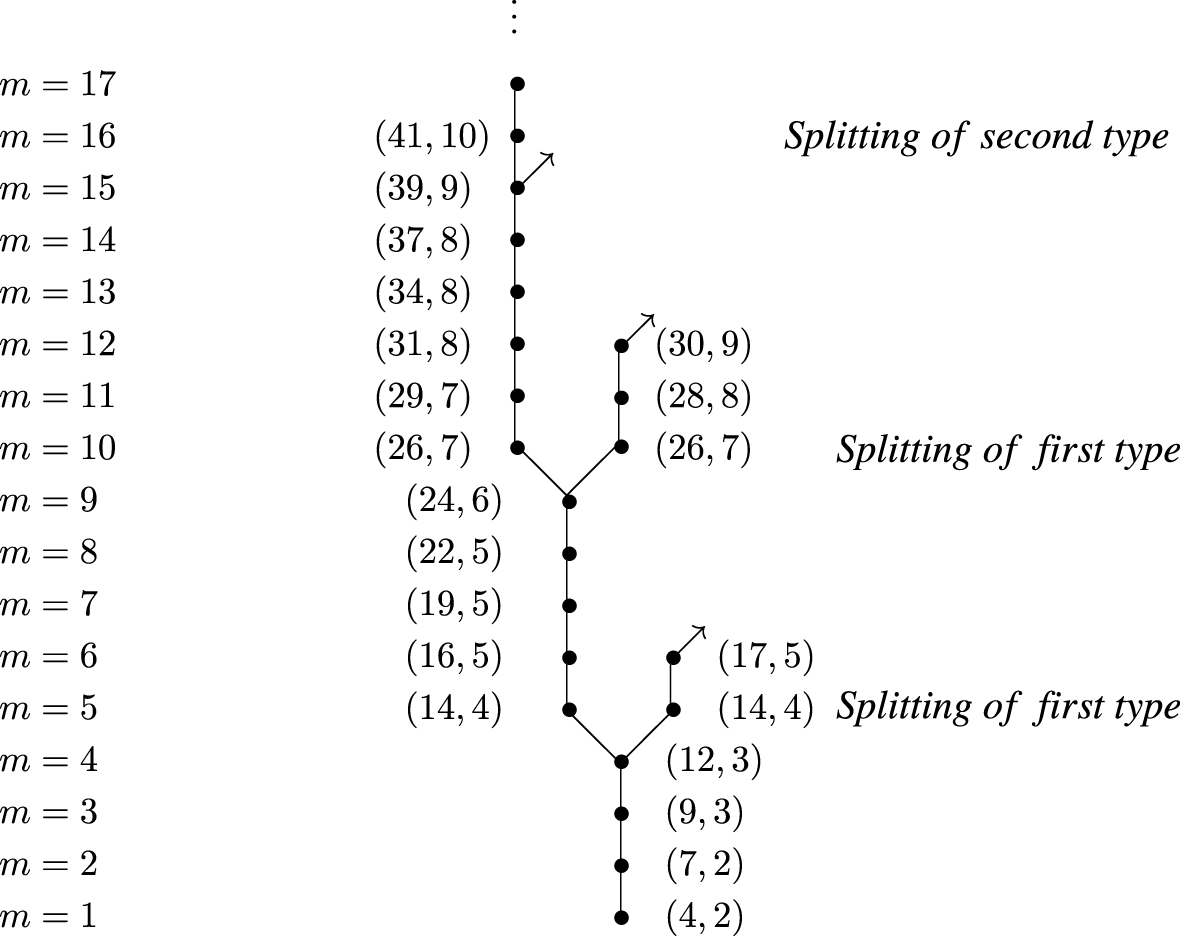
We will describe the irreducible decomposition of  $m$-jets through the singular locus as
 $$\begin{eqnarray}\left(\unicode[STIX]{x1D70B}_{m}^{-1}(X_{\text{Sing}})\right)_{\text{red}}=\mathop{\bigcup }_{\unicode[STIX]{x1D708}\in F_{m}}C_{m}^{\unicode[STIX]{x1D708}}\end{eqnarray}$$
for a certain finite set  $F_{m}\subseteq \mathbb{Z}^{2}$ and certain irreducible sets
 $C_{m}^{\unicode[STIX]{x1D708}}$ that we proceed to define. First we recall, in the case of only one characteristic exponent, some objects described in Section 3 in general.
The notion of equisingular dimension  $c$ was given in Definition 3.13. By Theorem 3.14 we have the following description of the singular locus of
 $X$ (recall that the characteristic exponent is
 $\unicode[STIX]{x1D6FE}=\big(a/n,b/n\big)$ with
 $a\geqslant b\geqslant 0$),
 $$\begin{eqnarray}\displaystyle X_{\text{Sing}}=\left\{\begin{array}{@{}cl@{}}\{z=x_{1}=0\} & \text{if }c=1~\big(\text{i.e. }b=0\big)\\ \{(0,0,0)\} & \text{if }c=2\text{ and }a=b=1\\ \{z=x_{1}=0\} & \text{if }c=2\text{ and }a>1,b=1\\ \{z=x_{1}=0\}\cup \{z=x_{2}=0\} & \text{if }c=2\text{ and }a,b>1.\end{array}\right. & & \displaystyle\end{eqnarray}$$
From Definition 3.17 we have that
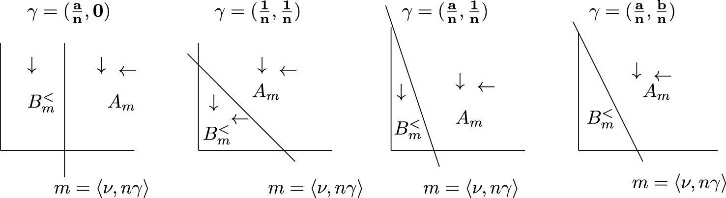
 $$\begin{eqnarray}\unicode[STIX]{x1D70E}_{\text{Sing}}=\left\{\begin{array}{@{}cl@{}}\stackrel{\circ }{\unicode[STIX]{x1D70E}} & \text{if }\unicode[STIX]{x1D6FE}=\big(\frac{1}{n},\frac{1}{n}\big)\\ \unicode[STIX]{x1D70E}\setminus \unicode[STIX]{x1D70C}_{2} & \text{if }\unicode[STIX]{x1D6FE}=\big(\frac{a}{n},\frac{1}{n}\big)\text{ or }\unicode[STIX]{x1D6FE}=\big(\frac{a}{n},0\big)\\ \unicode[STIX]{x1D70E}\setminus \{(0,0)\} & \text{otherwise}\end{array}\right.\end{eqnarray}$$
where recall that  $\unicode[STIX]{x1D70E}=\mathbb{R}_{{\geqslant}0}^{2}$ and
 $\unicode[STIX]{x1D70C}_{1}=(1,0)\mathbb{R}_{{\geqslant}0}$ and
 $\unicode[STIX]{x1D70C}_{2}=(0,1)\mathbb{R}_{{\geqslant}0}$ are its one-dimensional faces.
Given  $\unicode[STIX]{x1D6FE}(t)\,\in \,X_{m}$ with
 $x_{i}\circ \unicode[STIX]{x1D6FE}(t)\neq 0$ for
 $i=1,2$, we have that
 $\text{ord}_{t}(x_{i}\circ \unicode[STIX]{x1D6FE}(t))\geqslant 0$. Hence
 $$\begin{eqnarray}\unicode[STIX]{x1D708}:=\big(\text{ord}_{t}(x_{1}\circ \unicode[STIX]{x1D6FE}(t)),\text{ord}_{t}(x_{2}\circ \unicode[STIX]{x1D6FE}(t))\big)\in \unicode[STIX]{x1D70E}\,\cap \,N_{0}.\end{eqnarray}$$
If we add the condition  $\unicode[STIX]{x1D70B}_{m}(\unicode[STIX]{x1D6FE}(t))\,\in \,X_{\text{Sing}}$ then
 $\unicode[STIX]{x1D708}\,\in \,\unicode[STIX]{x1D70E}_{\text{Sing}}\,\cap \,N_{0}$. Moreover it is clear that
 $0\leqslant \unicode[STIX]{x1D708}_{i}\leqslant m$ for
 $i=1,2$.
Definition 4.4. Given a positive integer  $m$ and
 $\unicode[STIX]{x1D708}\in \unicode[STIX]{x1D70E}_{\text{Sing}}\cap \,[0,m]^{2}\cap \,N_{0}$, we define an algebraic variety
 $C_{m}^{\unicode[STIX]{x1D708}}\subseteq \mathbb{A}_{m}^{3}$ as follows (recall Remark 2.5).
 $\bullet$ If
 $m<\langle \unicode[STIX]{x1D708},n\unicode[STIX]{x1D6FE}\rangle$,
 $$\begin{eqnarray}C_{m}^{\unicode[STIX]{x1D708}}:=V\left(x_{1}^{(0)},\ldots ,x_{1}^{(\unicode[STIX]{x1D708}_{1}-1)},x_{2}^{(0)},\ldots ,x_{2}^{(\unicode[STIX]{x1D708}_{2}-1)},z^{(0)},\ldots ,z^{([m/n])}\right).\end{eqnarray}$$
Note that  $C_{m}^{\unicode[STIX]{x1D708}}$ is a nonsingular algebraic variety of
 $\mathbb{A}_{m}^{3}$.
 $\bullet$ If
 $m=\langle \unicode[STIX]{x1D708},n\unicode[STIX]{x1D6FE}\rangle$ and
 $\unicode[STIX]{x1D708}\,\in \,N$,
 $$\begin{eqnarray}C_{\langle \unicode[STIX]{x1D708},n\unicode[STIX]{x1D6FE}\rangle }^{\unicode[STIX]{x1D708}}:=V\left(x_{1}^{(0)},\ldots ,x_{1}^{(\unicode[STIX]{x1D708}_{1}-1)},x_{2}^{(0)},\ldots ,x_{2}^{(\unicode[STIX]{x1D708}_{2}-1)},z^{(0)},\ldots ,z^{(\langle \unicode[STIX]{x1D708},\unicode[STIX]{x1D6FE}\rangle -1)},F^{(\langle \unicode[STIX]{x1D708},n\unicode[STIX]{x1D6FE}\rangle )}\right).\end{eqnarray}$$
Note that  $C_{m}^{\unicode[STIX]{x1D708}}$ is not well defined if
 $\unicode[STIX]{x1D708}\,\in \,N_{0}\setminus N$ since
 $\langle \unicode[STIX]{x1D708},\unicode[STIX]{x1D6FE}\rangle$ is not an integer.
The polynomial  $F^{(\langle \unicode[STIX]{x1D708},n\unicode[STIX]{x1D6FE}\rangle )}$ modulo the ideal
 $$\begin{eqnarray}\big(x_{1}^{(0)},\ldots ,x_{1}^{(\unicode[STIX]{x1D708}_{1}-1)},x_{2}^{(0)},\ldots ,x_{2}^{(\unicode[STIX]{x1D708}_{2}-1)},z^{(0)},\ldots ,z^{(\langle \unicode[STIX]{x1D708},\unicode[STIX]{x1D6FE}\rangle -1)}\big)\end{eqnarray}$$
is studied in Lemma 4.5, and it turns out that  $C_{\langle \unicode[STIX]{x1D708},n\unicode[STIX]{x1D6FE}\rangle }^{\unicode[STIX]{x1D708}}$ is a singular algebraic variety of
 $\mathbb{A}_{m}^{3}$.
 $\bullet$ If
 $m>\langle \unicode[STIX]{x1D708},n\unicode[STIX]{x1D6FE}\rangle$ and
 $\unicode[STIX]{x1D708}\,\in \,N$,
 $$\begin{eqnarray}C_{m}^{\unicode[STIX]{x1D708}}:=\overline{\unicode[STIX]{x1D70B}_{m,\langle \unicode[STIX]{x1D708},n\unicode[STIX]{x1D6FE}\rangle }^{-1}\big(\text{Reg}\,(C_{\langle \unicode[STIX]{x1D708},n\unicode[STIX]{x1D6FE}\rangle }^{\unicode[STIX]{x1D708}})\big)}\end{eqnarray}$$
where the overline denotes the Zariski closure and Reg stands for regular locus.
It turns out to be crucial to understand the variety  $C_{\langle \unicode[STIX]{x1D708},n\unicode[STIX]{x1D6FE}\rangle }^{\unicode[STIX]{x1D708}}$.
Lemma 4.5. For  $\unicode[STIX]{x1D708}\,\in \,\unicode[STIX]{x1D70E}_{\text{Sing}}\,\cap \,N$ we define
 $$\begin{eqnarray}F_{\unicode[STIX]{x1D708}}^{(\langle \unicode[STIX]{x1D708},n\unicode[STIX]{x1D6FE}\rangle )}={z^{(\langle \unicode[STIX]{x1D708},\unicode[STIX]{x1D6FE}\rangle )}}^{n}-{x_{1}^{(\unicode[STIX]{x1D708}_{1})}}^{a}{x_{2}^{(\unicode[STIX]{x1D708}_{2})}}^{b}+\sum c_{ijk}\,{x_{1}^{(\unicode[STIX]{x1D708}_{1})}}^{i}{x_{2}^{(\unicode[STIX]{x1D708}_{2})}}^{j}{z^{(\langle \unicode[STIX]{x1D708},\unicode[STIX]{x1D6FE}\rangle )}}^{k}\end{eqnarray}$$
where the sum runs over  $i,j,k$ subject to the conditions: the monomial
 $c_{ijk}x_{1}^{i}x_{2}^{j}z^{k}$ appears in the q.o. polynomial
 $f$ and
 $\langle \unicode[STIX]{x1D708},(i,j)+k\unicode[STIX]{x1D6FE}\rangle =\langle \unicode[STIX]{x1D708},n\unicode[STIX]{x1D6FE}\rangle$. Note that, if
 $\unicode[STIX]{x1D708}\in \,\stackrel{\circ }{\unicode[STIX]{x1D70E}}$, the sum
 $\sum c_{ijk}{x_{1}^{(\unicode[STIX]{x1D708}_{1})}}^{i}{x_{2}^{(\unicode[STIX]{x1D708}_{2})}}^{j}{z^{(\langle \unicode[STIX]{x1D708},\unicode[STIX]{x1D6FE}\rangle )}}^{k}$ in
 $F_{\unicode[STIX]{x1D708}}^{(\langle \unicode[STIX]{x1D708},n\unicode[STIX]{x1D6FE}\rangle )}$ is zero.
We have that
 $$\begin{eqnarray}F^{(\langle \unicode[STIX]{x1D708},n\unicode[STIX]{x1D6FE}\rangle )}\equiv F_{\unicode[STIX]{x1D708}}^{(\langle \unicode[STIX]{x1D708},n\unicode[STIX]{x1D6FE}\rangle )}~\text{mod}~\big(x_{1}^{(0)},\ldots ,x_{1}^{(\unicode[STIX]{x1D708}_{1}-1)},x_{2}^{(0)},\ldots ,x_{2}^{(\unicode[STIX]{x1D708}_{2}-1)},z^{(0)},\ldots ,z^{(\langle \unicode[STIX]{x1D708},\unicode[STIX]{x1D6FE}\rangle -1)}\big),\end{eqnarray}$$
and hence
 $$\begin{eqnarray}C_{\langle \unicode[STIX]{x1D708},n\unicode[STIX]{x1D6FE}\rangle }^{\unicode[STIX]{x1D708}}=V\big(x_{1}^{(0)},\ldots ,x_{1}^{(\unicode[STIX]{x1D708}_{1}-1)},x_{2}^{(0)},\ldots ,x_{2}^{(\unicode[STIX]{x1D708}_{2}-1)},z^{(0)},\ldots ,z^{(\langle \unicode[STIX]{x1D708},\unicode[STIX]{x1D6FE}\rangle -1)},F_{\unicode[STIX]{x1D708}}^{(\langle \unicode[STIX]{x1D708},n\unicode[STIX]{x1D6FE}\rangle )}\big).\end{eqnarray}$$
In particular observe that  $F_{\unicode[STIX]{x1D708}}^{(\langle \unicode[STIX]{x1D708},n\unicode[STIX]{x1D6FE}\rangle )}$ is a q.o. polynomial in
 $R_{\unicode[STIX]{x1D708}}[z^{(\langle \unicode[STIX]{x1D708},\unicode[STIX]{x1D6FE}\rangle )}]$ (see Definition 3.19).
If  $\unicode[STIX]{x1D708}\,\in \,\unicode[STIX]{x1D70E}_{\text{Sing}}\,\cap \,\big(N_{0}\setminus N\big)$ we define
 $$\begin{eqnarray}F_{\unicode[STIX]{x1D708}}^{(\langle \unicode[STIX]{x1D708},n\unicode[STIX]{x1D6FE}\rangle )}=-{x_{1}^{(\unicode[STIX]{x1D708}_{1})}}^{a}{x_{2}^{(\unicode[STIX]{x1D708}_{2})}}^{b}+\sum c_{ij0}{x_{1}^{(\unicode[STIX]{x1D708}_{1})}}^{i}{x_{2}^{(\unicode[STIX]{x1D708}_{2})}}^{j}\end{eqnarray}$$
where  $c_{ij0}x_{1}^{i}x_{2}^{j}$ is a monomial in
 $f$ and
 $\langle \unicode[STIX]{x1D708},(i,j)\rangle =\langle \unicode[STIX]{x1D708},n\unicode[STIX]{x1D6FE}\rangle$. Then
 $$\begin{eqnarray}F^{(\langle \unicode[STIX]{x1D708},n\unicode[STIX]{x1D6FE}\rangle )}\equiv F_{\unicode[STIX]{x1D708}}^{(\langle \unicode[STIX]{x1D708},n\unicode[STIX]{x1D6FE}\rangle )}~\text{mod}~\big(x_{1}^{(0)},\ldots ,x_{1}^{(\unicode[STIX]{x1D708}_{1}-1)},x_{2}^{(0)},\ldots ,x_{2}^{(\unicode[STIX]{x1D708}_{2}-1)},z^{(0)},\ldots ,z^{([\langle \unicode[STIX]{x1D708},n\unicode[STIX]{x1D6FE}\rangle ])}\big).\end{eqnarray}$$
The sum  $\sum c_{ij0}{x_{1}^{(\unicode[STIX]{x1D708}_{1})}}^{i}{x_{2}^{(\unicode[STIX]{x1D708}_{2})}}^{j}$ is nonzero if and only if
 $\unicode[STIX]{x1D708}\,\in \,\unicode[STIX]{x1D70C}_{1}\cup \unicode[STIX]{x1D70C}_{2}$. Moreover, if
 $\unicode[STIX]{x1D708}\,\in \,\unicode[STIX]{x1D70C}_{1}\cup \unicode[STIX]{x1D70C}_{2}$
 $$\begin{eqnarray}F_{\unicode[STIX]{x1D708}}^{(\langle \unicode[STIX]{x1D708},n\unicode[STIX]{x1D6FE}\rangle )}=-{x_{1}^{(\unicode[STIX]{x1D708}_{1})}}^{a}{x_{2}^{(\unicode[STIX]{x1D708}_{2})}}^{b}\cdot U\end{eqnarray}$$
where  $U$ is a unit in
 $R_{\unicode[STIX]{x1D708}}$.
Proof. If  $\unicode[STIX]{x1D708}\,\in \,N$, we have by definition that the polynomial
 $F^{(\langle \unicode[STIX]{x1D708},n\unicode[STIX]{x1D6FE}\rangle )}$ modulo the ideal
 $\big(x_{1}^{(0)},\ldots ,x_{1}^{(\unicode[STIX]{x1D708}_{1}-1)},x_{2}^{(0)},\ldots ,x_{2}^{(\unicode[STIX]{x1D708}_{2}-1)},z^{(0)},\ldots ,z^{(\langle \unicode[STIX]{x1D708},\unicode[STIX]{x1D6FE}\rangle -1)}\big)$ is of the form
 $$\begin{eqnarray}{z^{(\langle \unicode[STIX]{x1D708},\unicode[STIX]{x1D6FE}\rangle )}}^{n}-{x_{1}^{(\unicode[STIX]{x1D708}_{1})}}^{a}{x_{2}^{(\unicode[STIX]{x1D708}_{2})}}^{b}+\sum c_{ijk}~{x_{1}^{(\unicode[STIX]{x1D6FC})}}^{i}{x_{2}^{(\unicode[STIX]{x1D6FD})}}^{j}{z^{(\unicode[STIX]{x1D6FF})}}^{k}\end{eqnarray}$$
where the sum runs subject to the conditions
 $$\begin{eqnarray}\displaystyle & & \displaystyle (i,j)+k\unicode[STIX]{x1D6FE}>n\unicode[STIX]{x1D6FE}\nonumber\\ \displaystyle & & \displaystyle i\unicode[STIX]{x1D6FC}+j\unicode[STIX]{x1D6FD}+k\unicode[STIX]{x1D6FF}=\langle \unicode[STIX]{x1D708},n\unicode[STIX]{x1D6FE}\rangle \nonumber\\ \displaystyle & & \displaystyle \unicode[STIX]{x1D6FC}\geqslant \unicode[STIX]{x1D708}_{1},\quad \unicode[STIX]{x1D6FD}\geqslant \unicode[STIX]{x1D708}_{2},\quad \unicode[STIX]{x1D6FF}\geqslant \langle \unicode[STIX]{x1D708},\unicode[STIX]{x1D6FE}\rangle .\nonumber\end{eqnarray}$$
If there exists at least one  $c_{ijk}\neq 0$ under these conditions
 $$\begin{eqnarray}\langle \unicode[STIX]{x1D708},n\unicode[STIX]{x1D6FE}\rangle =i\unicode[STIX]{x1D6FC}+j\unicode[STIX]{x1D6FD}+k\unicode[STIX]{x1D6FF}\geqslant i\unicode[STIX]{x1D708}_{1}+j\unicode[STIX]{x1D708}_{2}+k\langle \unicode[STIX]{x1D708},\unicode[STIX]{x1D6FE}\rangle =\langle \unicode[STIX]{x1D708},(i,j)+k\unicode[STIX]{x1D6FE}\rangle \geqslant \langle \unicode[STIX]{x1D708},n\unicode[STIX]{x1D6FE}\rangle ,\end{eqnarray}$$
then all inequalities must be equalities and we deduce that
 $$\begin{eqnarray}\unicode[STIX]{x1D6FC}=\unicode[STIX]{x1D708}_{1},\qquad \unicode[STIX]{x1D6FD}=\unicode[STIX]{x1D708}_{2}\qquad \text{and}\qquad \unicode[STIX]{x1D6FF}=\langle \unicode[STIX]{x1D708},\unicode[STIX]{x1D6FE}\rangle .\end{eqnarray}$$
Then, the condition  $i\unicode[STIX]{x1D6FC}+j\unicode[STIX]{x1D6FD}+k\unicode[STIX]{x1D6FF}=\langle \unicode[STIX]{x1D708},n\unicode[STIX]{x1D6FE}\rangle$ is
 $\langle \unicode[STIX]{x1D708},(i,j)+k\unicode[STIX]{x1D6FE}\rangle =\langle \unicode[STIX]{x1D708},n\unicode[STIX]{x1D6FE}\rangle$, and this only holds if
 $\unicode[STIX]{x1D708}\,\in \,\unicode[STIX]{x1D70C}_{1}\cup \unicode[STIX]{x1D70C}_{2}$.
If  $\unicode[STIX]{x1D708}\,\in \,N_{0}\setminus N$, first note that
 $$\begin{eqnarray}[\langle \unicode[STIX]{x1D708},\unicode[STIX]{x1D6FE}\rangle ]<\langle \unicode[STIX]{x1D708},\unicode[STIX]{x1D6FE}\rangle <[\langle \unicode[STIX]{x1D708},\unicode[STIX]{x1D6FE}\rangle ]+1.\end{eqnarray}$$
By definition  $F^{(\langle \unicode[STIX]{x1D708},n\unicode[STIX]{x1D6FE}\rangle )}\text{ mod }\big(x_{1}^{(0)},\ldots ,x_{1}^{(\unicode[STIX]{x1D708}_{1}-1)},x_{2}^{(0)},\ldots ,x_{2}^{(\unicode[STIX]{x1D708}_{2}-1)},z^{(0)},\ldots ,z^{([\langle \unicode[STIX]{x1D708},\unicode[STIX]{x1D6FE}\rangle ])}\big)$ is of the form
 $$\begin{eqnarray}-{x_{1}^{(\unicode[STIX]{x1D708}_{1})}}^{a}{x_{2}^{(\unicode[STIX]{x1D708}_{2})}}^{b}+\sum c_{ijk}{x_{1}^{(\unicode[STIX]{x1D6FC})}}^{i}{x_{2}^{(\unicode[STIX]{x1D6FD})}}^{j}{z^{(\unicode[STIX]{x1D6FF})}}^{k}\end{eqnarray}$$
where the sum runs subject to the conditions
 $$\begin{eqnarray}\displaystyle & & \displaystyle (i,j)+k\unicode[STIX]{x1D6FE}>n\unicode[STIX]{x1D6FE}\nonumber\\ \displaystyle & & \displaystyle i\unicode[STIX]{x1D6FC}+j\unicode[STIX]{x1D6FD}+k\unicode[STIX]{x1D6FF}=\langle \unicode[STIX]{x1D708},n\unicode[STIX]{x1D6FE}\rangle \nonumber\\ \displaystyle & & \displaystyle \unicode[STIX]{x1D6FC}\geqslant \unicode[STIX]{x1D708}_{1},~\unicode[STIX]{x1D6FD}\geqslant \unicode[STIX]{x1D708}_{2},~\unicode[STIX]{x1D6FF}\geqslant [\langle \unicode[STIX]{x1D708},\unicode[STIX]{x1D6FE}\rangle ]+1.\nonumber\end{eqnarray}$$
If there exists at least one  $c_{ijk}\neq 0$ with
 $i,j,k$ under these conditions and moreover with
 $k>0$, then
 $$\begin{eqnarray}\displaystyle \langle \unicode[STIX]{x1D708},n\unicode[STIX]{x1D6FE}\rangle & = & \displaystyle i\unicode[STIX]{x1D6FC}+j\unicode[STIX]{x1D6FD}+k\unicode[STIX]{x1D6FF}\geqslant i\unicode[STIX]{x1D708}_{1}+j\unicode[STIX]{x1D708}_{2}+k([\langle \unicode[STIX]{x1D708},\unicode[STIX]{x1D6FE}\rangle ]+1)\nonumber\\ \displaystyle & {>} & \displaystyle \langle \unicode[STIX]{x1D708},(i,j)+k\unicode[STIX]{x1D6FE}\rangle \geqslant \langle \unicode[STIX]{x1D708},n\unicode[STIX]{x1D6FE}\rangle .\nonumber\end{eqnarray}$$
Therefore we must have  $k=0$, and then
 $$\begin{eqnarray}\langle \unicode[STIX]{x1D708},n\unicode[STIX]{x1D6FE}\rangle =i\unicode[STIX]{x1D6FC}+j\unicode[STIX]{x1D6FD}\geqslant \langle \unicode[STIX]{x1D708},(i,j)\rangle \geqslant \langle \unicode[STIX]{x1D708},n\unicode[STIX]{x1D6FE}\rangle .\end{eqnarray}$$
Hence  $\unicode[STIX]{x1D6FC}=\unicode[STIX]{x1D708}_{1}$ and
 $\unicode[STIX]{x1D6FD}=\unicode[STIX]{x1D708}_{2}$. As in the case
 $\unicode[STIX]{x1D708}\,\in \,N$, the sum
 $\sum c_{ij0}{x_{1}^{(\unicode[STIX]{x1D708}_{1})}}^{i}{x_{2}^{(\unicode[STIX]{x1D708}_{2})}}^{j}$ is nonzero if and only if
 $\unicode[STIX]{x1D708}\,\in \,\unicode[STIX]{x1D70C}_{1}\cup \unicode[STIX]{x1D70C}_{2}$ since the conditions
 $(i,j)>n\unicode[STIX]{x1D6FE}$ and
 $\langle \unicode[STIX]{x1D708},(i,j)\rangle =\langle \unicode[STIX]{x1D708},n\unicode[STIX]{x1D6FE}\rangle$ are compatible if and only if
 $\unicode[STIX]{x1D708}\,\in \,\unicode[STIX]{x1D70E}_{\text{Sing}}\,\cap \,(\unicode[STIX]{x1D70C}_{1}\cup \unicode[STIX]{x1D70C}_{2})$.
If  $\unicode[STIX]{x1D708}\,\in \,\unicode[STIX]{x1D70C}_{1}$ then
 $F_{\unicode[STIX]{x1D708}}^{(\langle \unicode[STIX]{x1D708},n\unicode[STIX]{x1D6FE}\rangle )}=-{x_{1}^{(\unicode[STIX]{x1D708}_{1})}}^{a}{x_{2}^{(0)}}^{b}+\sum c_{ij0}{x_{1}^{(\unicode[STIX]{x1D708}_{1})}}^{i}{x_{2}^{(0)}}^{j}$ with the conditions
 $(i,j)>(a,b)$ and
 $\langle \unicode[STIX]{x1D708},n\unicode[STIX]{x1D6FE}\rangle =\langle \unicode[STIX]{x1D708},(i,j)\rangle$. Then
 $i=a$, and therefore
 $j>b$. Hence
 $$\begin{eqnarray}F_{\unicode[STIX]{x1D708}}^{(\langle \unicode[STIX]{x1D708},n\unicode[STIX]{x1D6FE}\rangle )}=-{x_{1}^{(\unicode[STIX]{x1D708}_{1})}}^{a}{x_{2}^{(0)}}^{b}\left(1+\sum c_{ij0}{x_{2}^{(0)}}^{j-b}\right)\end{eqnarray}$$
and  $1+\sum c_{ij0}{x_{2}^{(0)}}^{j-b}$ is a unit in
 $\mathbb{C}\{x_{2}^{(0)}\}$.
If  $\unicode[STIX]{x1D708}\,\in \,\unicode[STIX]{x1D70C}_{2}$ the proof is analogous, simply noticing (by the definition of
 $g_{2}$) that, since
 $\unicode[STIX]{x1D708}\,\in \,\unicode[STIX]{x1D70E}_{\text{Sing}}$, we must be in the case
 $b>1$.◻
Example 4.6. Consider the q.o. surface defined by  $f=z^{2}-x_{1}^{4}x_{2}^{3}+x_{1}^{2}x_{2}^{2}z$, with characteristic exponent
 $\unicode[STIX]{x1D706}=\big(\frac{4}{2},\frac{3}{2}\big)$. For
 $\unicode[STIX]{x1D708}=(2,0)$ we have
 $$\begin{eqnarray}F_{\unicode[STIX]{x1D708}}^{(8)}={z^{(4)}}^{2}-{x_{1}^{(2)}}^{4}{x_{2}^{(0)}}^{3}+{x_{1}^{(2)}}^{2}{x_{2}^{(0)}}^{2}z^{(4)}.\end{eqnarray}$$
Obviously we cannot write  $F_{\unicode[STIX]{x1D708}}^{(8)}$ as
 ${z^{(4)}}^{2}-{x_{1}^{(2)}}^{4}{x_{2}^{(0)}}^{3}\cdot U$ with
 $U$ a unit, as we have proved in Lemma 4.5 that it is the case when
 $\unicode[STIX]{x1D708}\notin N$. Notice however that
 $$\begin{eqnarray}V\big(F_{\unicode[STIX]{x1D708}}^{(8)}\big)\,\cap \,\{x_{1}^{(2)}\neq 0\}\,\cap \,\{x_{2}^{(0)}\neq 0\}\subseteq \{z^{(4)}\neq 0\},\end{eqnarray}$$
this will turn out to be crucial (see Corollary 5.16 for a complete statement in the general case).
To understand completely the sets  $C_{m}^{\unicode[STIX]{x1D708}}$ for
 $m>\langle \unicode[STIX]{x1D708},n\unicode[STIX]{x1D6FE}\rangle$, we need to study the regular part Reg
 $\big(C_{\langle \unicode[STIX]{x1D708},n\unicode[STIX]{x1D6FE}\rangle }^{\unicode[STIX]{x1D708}}\big)$. It is closely related to the regular locus of
 $X$, described in (11).
Lemma 4.7. For  $\unicode[STIX]{x1D708}\,\in \,\unicode[STIX]{x1D70E}_{\text{Sing}}\,\cap \,N$, let us denote
 $$\begin{eqnarray}J^{\unicode[STIX]{x1D708}}=\big(x_{1}^{(0)},\ldots ,x_{1}^{(\unicode[STIX]{x1D708}_{1}-1)},x_{2}^{(0)},\ldots ,x_{2}^{(\unicode[STIX]{x1D708}_{2}-1)},z^{(0)},\ldots ,z^{(\langle \unicode[STIX]{x1D708},\unicode[STIX]{x1D6FE}\rangle -1)}\big).\end{eqnarray}$$
We have:
(i) if
$\unicode[STIX]{x1D6FE}=(1/n,1/n)$, and, as a consequence, for$$\begin{eqnarray}\overline{\text{Reg}\,\big(C_{\langle \unicode[STIX]{x1D708},n\unicode[STIX]{x1D6FE}\rangle }^{\unicode[STIX]{x1D708}}\big)}=C_{\langle \unicode[STIX]{x1D708},n\unicode[STIX]{x1D6FE}\rangle }^{\unicode[STIX]{x1D708}}\end{eqnarray}$$$m>\langle \unicode[STIX]{x1D708},n\unicode[STIX]{x1D6FE}\rangle$, $$\begin{eqnarray}C_{m}^{\unicode[STIX]{x1D708}}=V\big(J^{\unicode[STIX]{x1D708}},F^{(\langle \unicode[STIX]{x1D708},n\unicode[STIX]{x1D6FE}\rangle )},\ldots ,F^{(m)}\big).\end{eqnarray}$$(ii) Otherwise
$\unicode[STIX]{x1D6FE}=(a/n,b/n)$ with $a>1$ and As a consequence, for$$\begin{eqnarray}\text{Reg}\,\big(C_{\langle \unicode[STIX]{x1D708},n\unicode[STIX]{x1D6FE}\rangle }^{\unicode[STIX]{x1D708}}\big)=\left\{\begin{array}{@{}cl@{}}C_{\langle \unicode[STIX]{x1D708},n\unicode[STIX]{x1D6FE}\rangle }^{\unicode[STIX]{x1D708}}\,\cap \,\{x_{1}^{(\unicode[STIX]{x1D708}_{1})}\neq 0\} & \text{if }b\in \{0,1\}\\ C_{\langle \unicode[STIX]{x1D708},n\unicode[STIX]{x1D6FE}\rangle }^{\unicode[STIX]{x1D708}}\,\cap \,\{x_{1}^{(\unicode[STIX]{x1D708}_{1})}\neq 0\}\,\cap \,\{x_{2}^{(\unicode[STIX]{x1D708}_{2})}\neq 0\} & \text{otherwise}.\end{array}\right.\end{eqnarray}$$$m>\langle \unicode[STIX]{x1D708},n\unicode[STIX]{x1D6FE}\rangle$ and $b=0$ or $1$, we have that while for$$\begin{eqnarray}C_{m}^{\unicode[STIX]{x1D708}}=\overline{V\left(J^{\unicode[STIX]{x1D708}},F^{(\langle \unicode[STIX]{x1D708},n\unicode[STIX]{x1D6FE}\rangle )},\ldots ,F^{(m)}\right)\,\cap \,\{x_{1}^{(\unicode[STIX]{x1D708}_{1})}\neq 0\}}\end{eqnarray}$$$m>\langle \unicode[STIX]{x1D708},n\unicode[STIX]{x1D6FE}\rangle$ and $b\neq 0,1$, $$\begin{eqnarray}C_{m}^{\unicode[STIX]{x1D708}}=\overline{V\left(J^{\unicode[STIX]{x1D708}},F^{(\langle \unicode[STIX]{x1D708},n\unicode[STIX]{x1D6FE}\rangle )},\ldots ,F^{(m)}\right)\,\cap \,\{x_{1}^{(\unicode[STIX]{x1D708}_{1})}\neq 0\}\,\cap \,\{x_{2}^{(\unicode[STIX]{x1D708}_{2})}\neq 0\}}.\end{eqnarray}$$


Proof. We distinguish cases according to the description in (11) of the singular locus.
(i) If
$\unicode[STIX]{x1D6FE}=(1/n,1/n)$ the claim of the Lemma is clear, since the singular locus of such a q.o. surface is the origin.(ii) If
$\unicode[STIX]{x1D6FE}=(a/n,0)$ we have to prove that, in $C_{\langle \unicode[STIX]{x1D708},n\unicode[STIX]{x1D6FE}\rangle }^{\unicode[STIX]{x1D708}}$, the conditions $x_{1}^{(\unicode[STIX]{x1D708}_{1})}\neq 0$ and $z^{(\langle \unicode[STIX]{x1D708},\unicode[STIX]{x1D6FE}\rangle )}\neq 0$ are equivalent. By Lemma 4.5, is a defining equation of$$\begin{eqnarray}F_{\unicode[STIX]{x1D708}}^{(\langle \unicode[STIX]{x1D708},n\unicode[STIX]{x1D6FE}\rangle )}={z^{(\langle \unicode[STIX]{x1D708},\unicode[STIX]{x1D6FE}\rangle )}}^{n}-{x_{1}^{(\unicode[STIX]{x1D708}_{1})}}^{a}+\sum c_{ijk}{x_{1}^{(\unicode[STIX]{x1D708}_{1})}}^{i}{x_{2}^{(\unicode[STIX]{x1D708}_{2})}}^{j}{z^{(\langle \unicode[STIX]{x1D708},\unicode[STIX]{x1D6FE}\rangle )}}^{k}\end{eqnarray}$$$C_{\langle \unicode[STIX]{x1D708},n\unicode[STIX]{x1D6FE}\rangle }^{\unicode[STIX]{x1D708}}$. If the sum in $F_{\unicode[STIX]{x1D708}}^{(\langle \unicode[STIX]{x1D708},n\unicode[STIX]{x1D6FE}\rangle )}$ is empty the claim is obvious. Otherwise $\unicode[STIX]{x1D708}\,\in \,\unicode[STIX]{x1D70C}_{1}\cup \unicode[STIX]{x1D70C}_{2}$ and, since $\unicode[STIX]{x1D708}\,\in \,\unicode[STIX]{x1D70E}_{\text{Sing}}$, we deduce that $\unicode[STIX]{x1D708}\,\in \,\unicode[STIX]{x1D70C}_{1}$. Then with$$\begin{eqnarray}F_{\unicode[STIX]{x1D708}}^{(\langle \unicode[STIX]{x1D708},n\unicode[STIX]{x1D6FE}\rangle )}={z^{(\langle \unicode[STIX]{x1D708},\unicode[STIX]{x1D6FE}\rangle )}}^{n}-{x_{1}^{(\unicode[STIX]{x1D708}_{1})}}^{a}+\sum c_{ijk}{x_{1}^{(\unicode[STIX]{x1D708}_{1})}}^{i}{x_{2}^{(0)}}^{j}{z^{(\langle \unicode[STIX]{x1D708},\unicode[STIX]{x1D6FE}\rangle )}}^{k}\end{eqnarray}$$$\langle \unicode[STIX]{x1D708},(i,j)+k\unicode[STIX]{x1D6FE}\rangle =\langle \unicode[STIX]{x1D708},n\unicode[STIX]{x1D6FE}\rangle$, or equivalently This implies that$$\begin{eqnarray}\unicode[STIX]{x1D708}_{1}\left(i+k\frac{a}{n}\right)=\unicode[STIX]{x1D708}_{1}n\frac{a}{n}.\end{eqnarray}$$$i+k(a/n)=a$, and since $0\leqslant k<n$ and $\text{gcd}(a,n)=1$, we deduce that $i=a$ and $k=0$. Then $j>0$ for any $c_{aj0}\neq 0$ and we can write $F_{\unicode[STIX]{x1D708}}^{(\langle \unicode[STIX]{x1D708},n\unicode[STIX]{x1D6FE}\rangle )}$ as Since$$\begin{eqnarray}\displaystyle F_{\unicode[STIX]{x1D708}}^{(\langle \unicode[STIX]{x1D708},n\unicode[STIX]{x1D6FE}\rangle )} & = & \displaystyle {z^{(\langle \unicode[STIX]{x1D708},\unicode[STIX]{x1D6FE}\rangle )}}^{n}-{x_{1}^{(\unicode[STIX]{x1D708}_{1})}}^{a}+\mathop{\sum }_{j}c_{aj0}{x_{1}^{(\unicode[STIX]{x1D708}_{1})}}^{a}{x_{2}^{(0)}}^{j}\nonumber\\ \displaystyle & = & \displaystyle {z^{(\langle \unicode[STIX]{x1D708},\unicode[STIX]{x1D6FE}\rangle )}}^{n}-{x_{1}^{(\unicode[STIX]{x1D708}_{1})}}^{a}\biggl(1+\mathop{\sum }_{j}c_{aj0}{x_{2}^{(0)}}^{j}\biggr).\nonumber\end{eqnarray}$$$1+\sum c_{aj0}{x_{2}^{(0)}}^{j}$ is a unit in $R_{\unicode[STIX]{x1D708}}=\mathbb{C}\{x_{2}^{(0)}\}[x_{1}^{(\unicode[STIX]{x1D708}_{1})}]$, it does not vanish, and the claim follows.(iii) If
$\unicode[STIX]{x1D6FE}=(a/n,1/n)$, by Lemma 4.5 we have that where the sum runs over$$\begin{eqnarray}F_{\unicode[STIX]{x1D708}}^{(\langle \unicode[STIX]{x1D708},n\unicode[STIX]{x1D6FE}\rangle )}={z^{(\langle \unicode[STIX]{x1D708},\unicode[STIX]{x1D6FE}\rangle )}}^{n}-{x_{1}^{(\unicode[STIX]{x1D708}_{1})}}^{a}x_{2}^{(\unicode[STIX]{x1D708}_{2})}+\sum c_{ijk}{x_{1}^{(\unicode[STIX]{x1D708}_{1})}}^{i}{x_{2}^{(\unicode[STIX]{x1D708}_{2})}}^{j}{z^{(\langle \unicode[STIX]{x1D708},\unicode[STIX]{x1D6FE}\rangle )}}^{k}\end{eqnarray}$$$(i,j,k)$ such that $(i,j)+k\unicode[STIX]{x1D6FE}>(a,1)$. Therefore we deduce that for any such $(i,j,k)$ we have $i>0$ because $0\leqslant k<n$. It follows that if $x_{1}^{(\unicode[STIX]{x1D708}_{1})}=0$ and $F_{\unicode[STIX]{x1D708}}^{(\langle \unicode[STIX]{x1D708},n\unicode[STIX]{x1D6FE}\rangle )}=0$ then we have that $z^{(\langle \unicode[STIX]{x1D708},\unicode[STIX]{x1D6FE}\rangle )}=0$. Hence $$\begin{eqnarray}\displaystyle \text{Reg}\,\big(C_{\langle \unicode[STIX]{x1D708},n\unicode[STIX]{x1D6FE}\rangle }^{\unicode[STIX]{x1D708}}\big) & = & \displaystyle C_{\langle \unicode[STIX]{x1D708},n\unicode[STIX]{x1D6FE}\rangle }^{\unicode[STIX]{x1D708}}\,\cap \,\{z^{(\langle \unicode[STIX]{x1D708},\unicode[STIX]{x1D6FE}\rangle )}\neq 0\}\bigcup \mathop{C}_{\langle \unicode[STIX]{x1D708},n\unicode[STIX]{x1D6FE}\rangle }^{\unicode[STIX]{x1D708}}\,\cap \,\{x_{1}^{(\unicode[STIX]{x1D708}_{1})}\neq 0\}\nonumber\\ \displaystyle & = & \displaystyle C_{\langle \unicode[STIX]{x1D708},n\unicode[STIX]{x1D6FE}\rangle }^{\unicode[STIX]{x1D708}}\,\cap \,\{x_{1}^{(\unicode[STIX]{x1D708}_{1})}\neq 0\}.\nonumber\end{eqnarray}$$(iv) If
$\unicode[STIX]{x1D6FE}=(a/n,b/n)$ with $b>1$, we have that and we claim that$$\begin{eqnarray}\text{Reg}\,\big(C_{\langle \unicode[STIX]{x1D708},n\unicode[STIX]{x1D6FE}\rangle }^{\unicode[STIX]{x1D708}}\big)=C_{\langle \unicode[STIX]{x1D708},n\unicode[STIX]{x1D6FE}\rangle }^{\unicode[STIX]{x1D708}}\,\cap \,\{x_{1}^{(\unicode[STIX]{x1D708}_{1})}\neq 0\}\,\cap \,\{x_{2}^{(\unicode[STIX]{x1D708}_{2})}\neq 0\}\bigcup \mathop{C}_{\langle \unicode[STIX]{x1D708},n\unicode[STIX]{x1D6FE}\rangle }^{\unicode[STIX]{x1D708}}\,\cap \,\{z^{(\langle \unicode[STIX]{x1D708},\unicode[STIX]{x1D6FE}\rangle )}\neq 0\}\end{eqnarray}$$$C_{\langle \unicode[STIX]{x1D708},n\unicode[STIX]{x1D6FE}\rangle }^{\unicode[STIX]{x1D708}}\,\cap \,\{z^{(\langle \unicode[STIX]{x1D708},\unicode[STIX]{x1D6FE}\rangle )}\neq 0\}=C_{\langle \unicode[STIX]{x1D708},n\unicode[STIX]{x1D6FE}\rangle }^{\unicode[STIX]{x1D708}}\,\cap \,\{x_{1}^{(\unicode[STIX]{x1D708}_{1})}\neq 0\}\,\cap \,\{x_{2}^{(\unicode[STIX]{x1D708}_{2})}\neq 0\}$. Indeed, by Lemma 4.5 it follows that is a defining equation of$$\begin{eqnarray}F_{\unicode[STIX]{x1D708}}^{(\langle \unicode[STIX]{x1D708},n\unicode[STIX]{x1D6FE}\rangle )}={z^{(\langle \unicode[STIX]{x1D708},\unicode[STIX]{x1D6FE}\rangle )}}^{n}-{x_{1}^{(\unicode[STIX]{x1D708}_{1})}}^{a}{x_{2}^{(\unicode[STIX]{x1D708}_{2})}}^{b}+\sum c_{ijk}~{x_{1}^{(\unicode[STIX]{x1D708}_{1})}}^{i}{x_{2}^{(\unicode[STIX]{x1D708}_{2})}}^{j}{z^{(\langle \unicode[STIX]{x1D708},\unicode[STIX]{x1D6FE}\rangle )}}^{k}\end{eqnarray}$$$C_{\langle \unicode[STIX]{x1D708},n\unicode[STIX]{x1D6FE}\rangle }^{\unicode[STIX]{x1D708}}$. If the sum is zero, the claim is obvious. Otherwise $\unicode[STIX]{x1D708}\,\in \,\unicode[STIX]{x1D70C}_{1}\cup \unicode[STIX]{x1D70C}_{2}$. Let us suppose that $\unicode[STIX]{x1D708}\,\in \,\unicode[STIX]{x1D70C}_{1}$ (the case $\unicode[STIX]{x1D708}\,\in \,\unicode[STIX]{x1D70C}_{2}$ is completely analogous). The monomials on the sum are of the form $c_{ijk}{x_{1}^{(\unicode[STIX]{x1D708}_{1})}}^{i}{x_{2}^{(0)}}^{j}{z^{(\langle \unicode[STIX]{x1D708},\unicode[STIX]{x1D6FE}\rangle )}}^{k}$ with $i+k(a/n)=a$ and $j+k(b/n)>b$. In particular we deduce that $i,j>0$. Therefore if $F_{\unicode[STIX]{x1D708}}^{(\langle \unicode[STIX]{x1D708},n\unicode[STIX]{x1D6FE}\rangle )}=0$ and either $x_{1}^{(\unicode[STIX]{x1D708}_{1})}=0$ or $x_{2}^{(0)}=0$ it follows that $z^{(\langle \unicode[STIX]{x1D708},\unicode[STIX]{x1D6FE}\rangle )}=0$. And conversely, if $z^{(\langle \unicode[STIX]{x1D708},\unicode[STIX]{x1D6FE}\rangle )}=0$, then with$$\begin{eqnarray}F_{\unicode[STIX]{x1D708}}^{(\langle \unicode[STIX]{x1D708},n\unicode[STIX]{x1D6FE}\rangle )}\big(z^{(\langle \unicode[STIX]{x1D708},\unicode[STIX]{x1D6FE}\rangle )}=0\big)=-{x_{1}^{(\unicode[STIX]{x1D708}_{1})}}^{a}{x_{2}^{(0)}}^{b}\cdot U\end{eqnarray}$$$U$ a unit in $\mathbb{C}\{x_{2}^{(0)}\}$ (because if we impose $k=0$ on the conditions $i+k(a/n)=a$ and $j+k(b/n)>b$ we obviously obtain $i=a$ and $j>b$). Then the result follows.◻


Definition 4.8. We define the set  $A_{m}\cup B_{m}\subseteq \unicode[STIX]{x1D70E}_{\text{Sing}}\,\cap \,[0,m]^{2}\,\cap \,N_{0}$ as
 $$\begin{eqnarray}\displaystyle & \displaystyle A_{m}=\{\unicode[STIX]{x1D708}\in \unicode[STIX]{x1D70E}_{\text{Sing}}\,\cap \,[0,m]^{2}\,\cap \,N_{0}~|~\langle \unicode[STIX]{x1D708},n\unicode[STIX]{x1D6FE}\rangle >m\} & \displaystyle \nonumber\\ \displaystyle & \displaystyle B_{m}=\{\unicode[STIX]{x1D708}\in \unicode[STIX]{x1D70E}_{\text{Sing}}\,\cap \,[0,m]^{2}\,\cap \,N~|~\langle \unicode[STIX]{x1D708},n\unicode[STIX]{x1D6FE}\rangle \leqslant m\}. & \displaystyle \nonumber\end{eqnarray}$$
Moreover, we decompose the set  $B_{m}$ as
 $B_{m}=B_{m}^{=}\cup B_{m}^{{<}}$, where
 $$\begin{eqnarray}\displaystyle & \displaystyle B_{m}^{=}=\{\unicode[STIX]{x1D708}\in \unicode[STIX]{x1D70E}_{\text{Sing}}\,\cap \,[0,m]^{2}\,\cap \,N~|~\langle \unicode[STIX]{x1D708},n\unicode[STIX]{x1D6FE}\rangle =m\} & \displaystyle \nonumber\\ \displaystyle & \displaystyle B_{m}^{{<}}=\{\unicode[STIX]{x1D708}\in \unicode[STIX]{x1D70E}_{\text{Sing}}\,\cap \,[0,m]^{2}\,\cap \,N~|~\langle \unicode[STIX]{x1D708},n\unicode[STIX]{x1D6FE}\rangle <m\}. & \displaystyle \nonumber\end{eqnarray}$$
Remark 4.9. Notice that, for  $m\,\in \,\mathbb{Z}_{{>}0}$, the set
 $B_{m}$ is
 $$\begin{eqnarray}\displaystyle B_{m} & = & \displaystyle \{\unicode[STIX]{x1D708}\in \unicode[STIX]{x1D70E}_{\text{Sing}}\,\cap \,[0,m]^{2}\,\cap \,N~|~a\unicode[STIX]{x1D708}_{1}+b\unicode[STIX]{x1D708}_{2}\leqslant m\}\nonumber\\ \displaystyle & = & \displaystyle \left\{\unicode[STIX]{x1D708}\in \unicode[STIX]{x1D70E}_{\text{Sing}}\,\cap \,[0,m]^{2}\,\cap \,N_{0}~|~\frac{a\unicode[STIX]{x1D708}_{1}+b\unicode[STIX]{x1D708}_{2}}{n}\in \mathbb{Z}\text{ and }a\unicode[STIX]{x1D708}_{1}+b\unicode[STIX]{x1D708}_{2}\leqslant m\right\}.\nonumber\end{eqnarray}$$
For any  $m>0$ and any
 $\unicode[STIX]{x1D708}\,\in \,A_{m}\cup B_{m}$, we have defined an algebraic variety
 $C_{m}^{\unicode[STIX]{x1D708}}$ in Definition 4.4. These are the candidates to be the irreducible components of
 $\big(\unicode[STIX]{x1D70B}_{m}^{-1}(X_{\text{Sing}})\big)_{\text{red}}$. To prove this assertion we need to make sure that these sets are irreducible, and that they cover
 $\big(\unicode[STIX]{x1D70B}_{m}^{-1}(X_{\text{Sing}})\big)_{\text{red}}$.
Lemma 4.10. For  $m\,\in \,\mathbb{Z}_{{>}0}$ and
 $\unicode[STIX]{x1D708}\,\in \,A_{m}\cup B_{m}$ we have that
 $C_{m}^{\unicode[STIX]{x1D708}}$ is irreducible. Moreover its codimension is:
 $$\begin{eqnarray}\text{Codim}\big(C_{m}^{\unicode[STIX]{x1D708}}\big)=\left\{\begin{array}{@{}cl@{}}\unicode[STIX]{x1D708}_{1}+\unicode[STIX]{x1D708}_{2}+\left[\frac{m}{n}\right] & \text{if }\unicode[STIX]{x1D708}\in A_{m}\\ \unicode[STIX]{x1D708}_{1}+\unicode[STIX]{x1D708}_{2}+\langle \unicode[STIX]{x1D708},\unicode[STIX]{x1D6FE}\rangle +m-\langle \unicode[STIX]{x1D708},n\unicode[STIX]{x1D6FE}\rangle +1 & \text{if }\unicode[STIX]{x1D708}\in B_{m}.\end{array}\right.\end{eqnarray}$$
Proof. For  $\unicode[STIX]{x1D708}\,\in \,A_{m}\cup B_{m}^{=}$ the claim is clear by definition and by Lemma 4.5. If
 $\unicode[STIX]{x1D708}\,\in \,B_{m}^{{<}}$ it follows by Proposition 2.4.◻
Lemma 4.11. For  $m\,\in \,\mathbb{Z}_{{>}0}$,
 $$\begin{eqnarray}\big(\unicode[STIX]{x1D70B}_{m}^{-1}(X_{\text{Sing}})\big)_{\text{red}}=\mathop{\bigcup }_{\unicode[STIX]{x1D708}\in A_{m}\cup B_{m}}C_{m}^{\unicode[STIX]{x1D708}}.\end{eqnarray}$$
Proof. By definition we have that  $\cup _{\unicode[STIX]{x1D708}\,\in \,A_{m}\cup B_{m}}C_{m}^{\unicode[STIX]{x1D708}}\subseteq \big(\unicode[STIX]{x1D70B}_{m}^{-1}(X_{\text{Sing}})\big)_{\text{red}}$. We have to prove that any
 $m$-jet
 $\unicode[STIX]{x1D6FE}(t)\,\in \,\big(\unicode[STIX]{x1D70B}_{m}^{-1}(X_{\text{Sing}})\big)_{\text{red}}$ belongs to certain
 $C_{m}^{\unicode[STIX]{x1D708}}$ with
 $\unicode[STIX]{x1D708}\,\in \,A_{m}\cup B_{m}$.
 $\bullet$ Suppose first that
 $x_{i}\circ \unicode[STIX]{x1D6FE}(t)\neq 0$ for
 $i=1,2$. Then we set
 $\unicode[STIX]{x1D708}:=\big(\text{ord}_{t}(x_{1}\circ \unicode[STIX]{x1D6FE}(t)),\text{ord}_{t}(x_{2}\circ \unicode[STIX]{x1D6FE}(t))\big)$. We have that
 $\unicode[STIX]{x1D708}\,\in \,\unicode[STIX]{x1D70E}_{\text{Sing}}\,\cap \,[0,m]^{2}\,\cap \,N_{0}$, and we only need to prove that if
 $\langle \unicode[STIX]{x1D708},n\unicode[STIX]{x1D6FE}\rangle \leqslant m$ then
 $\unicode[STIX]{x1D708}\,\in \,N$. Indeed, let us suppose the contrary, that
 $m\geqslant \langle \unicode[STIX]{x1D708},n\unicode[STIX]{x1D6FE}\rangle$ and
 $\unicode[STIX]{x1D708}\,\in \,N_{0}\setminus N$. We define the ideal
 $$\begin{eqnarray}J=\big(x_{1}^{(0)},\ldots ,x_{1}^{(\unicode[STIX]{x1D708}_{1}-1)},x_{2}^{(0)},\ldots ,x_{2}^{(\unicode[STIX]{x1D708}_{2}-1)}\big).\end{eqnarray}$$
Note that  $\unicode[STIX]{x1D6FE}(t)\,\in \,V(J)\,\cap \,\{x_{1}^{(\unicode[STIX]{x1D708}_{1})}\neq 0\}\,\cap \,\{x_{2}^{(\unicode[STIX]{x1D708}_{2})}\neq 0\}$. Using that
 $f\circ \unicode[STIX]{x1D6FE}(t)\equiv 0~\text{mod}~t^{m+1}$ we deduce that
 $$\begin{eqnarray}\unicode[STIX]{x1D6FE}(t)\in V\big(J+(z^{(0)},\ldots ,z^{([\langle \unicode[STIX]{x1D708},\unicode[STIX]{x1D6FE}\rangle ])})\big)\,\cap \,\{x_{1}^{(\unicode[STIX]{x1D708}_{1})}\neq 0\}\,\cap \,\{x_{2}^{(\unicode[STIX]{x1D708}_{2})}\neq 0\}\end{eqnarray}$$
and that
 $$\begin{eqnarray}\displaystyle F^{(\langle \unicode[STIX]{x1D708},n\unicode[STIX]{x1D6FE}\rangle )} & \equiv & \displaystyle -{x_{1}^{(\unicode[STIX]{x1D708}_{1})}}^{a}{x_{2}^{(\unicode[STIX]{x1D708}_{2})}}^{b}+\sum c_{ijk}{x_{1}^{(\unicode[STIX]{x1D708}_{1})}}^{i}{x_{2}^{(\unicode[STIX]{x1D708}_{2})}}^{j}{z^{([\langle \unicode[STIX]{x1D708},\unicode[STIX]{x1D6FE}\rangle ]+1)}}^{k}~\text{mod}~J\nonumber\\ \displaystyle & & \displaystyle +\,\big(z^{(0)},\ldots ,z^{([\langle \unicode[STIX]{x1D708},\unicode[STIX]{x1D6FE}\rangle ])}\big)\nonumber\end{eqnarray}$$
where the sum runs under the conditions  $(i,j)+k\unicode[STIX]{x1D6FE}>n\unicode[STIX]{x1D6FE}$ and
 $\langle \unicode[STIX]{x1D708},(i,j)\rangle +k([\langle \unicode[STIX]{x1D708},\unicode[STIX]{x1D6FE}\rangle ]+1)=\langle \unicode[STIX]{x1D708},n\unicode[STIX]{x1D6FE}\rangle$. But, since
 $\unicode[STIX]{x1D708}\notin N$ we have
 $[\langle \unicode[STIX]{x1D708},\unicode[STIX]{x1D6FE}\rangle ]+1>\langle \unicode[STIX]{x1D708},\unicode[STIX]{x1D6FE}\rangle$, and then
 $$\begin{eqnarray}\langle \unicode[STIX]{x1D708},(i,j)\rangle +k([\langle \unicode[STIX]{x1D708},\unicode[STIX]{x1D6FE}\rangle ]+1)>\langle \unicode[STIX]{x1D708},(i,j)+k\unicode[STIX]{x1D6FE}\rangle \geqslant \langle \unicode[STIX]{x1D708},n\unicode[STIX]{x1D6FE}\rangle\end{eqnarray}$$
and we deduce that  $F^{(\langle \unicode[STIX]{x1D708},n\unicode[STIX]{x1D6FE}\rangle )}\equiv -{x_{1}^{(\unicode[STIX]{x1D708}_{1})}}^{a}{x_{2}^{(\unicode[STIX]{x1D708}_{2})}}^{b}\text{ mod }J+\big(z^{(0)},\ldots ,z^{([\langle \unicode[STIX]{x1D708},\unicode[STIX]{x1D6FE}\rangle ])}\big)$. Since we have that
 ${x_{1}^{(\unicode[STIX]{x1D708}_{1})}}^{a}{x_{2}^{(\unicode[STIX]{x1D708}_{2})}}^{b}$ is nonzero, this contradicts the fact that
 $\unicode[STIX]{x1D6FE}(t)\,\in \,X_{m}$, because
 $\langle \unicode[STIX]{x1D708},n\unicode[STIX]{x1D6FE}\rangle \leqslant m$.
 $\bullet$ Suppose that
 $x_{1}\circ \unicode[STIX]{x1D6FE}(t)=0$ and
 $x_{2}\circ \unicode[STIX]{x1D6FE}(t)\neq 0$. We set
 $\unicode[STIX]{x1D708}_{2}:=\text{ord}_{t}\big(x_{2}\circ \unicode[STIX]{x1D6FE}(t)\big)\leqslant m$. Note that
 $\unicode[STIX]{x1D708}:=(m,\unicode[STIX]{x1D708}_{2})\,\in \,A_{m}$ and since
 $\unicode[STIX]{x1D6FE}(t)\,\in \,C_{m}^{\unicode[STIX]{x1D708}}$ we are done.
 $\bullet$ If
 $x_{1}\circ \unicode[STIX]{x1D6FE}(t)\neq 0$ and
 $x_{2}\circ \unicode[STIX]{x1D6FE}(t)=0$ then we set
 $\unicode[STIX]{x1D708}:=(\text{ord}_{t}(x_{1}\circ \unicode[STIX]{x1D6FE}(t)),m)$. We have that if
 $b\neq 0$ then
 $\langle \unicode[STIX]{x1D708},n\unicode[STIX]{x1D6FE}\rangle >m$ and therefore
 $\unicode[STIX]{x1D708}\,\in \,A_{m}$. If
 $b=0$ and
 $a\unicode[STIX]{x1D708}_{1}\leqslant m$ we can prove, arguing as in the case
 $x_{i}\circ \unicode[STIX]{x1D6FE}(t)\neq 0$ for
 $i=1,2$, that
 $\unicode[STIX]{x1D708}\,\in \,N$. Then
 $\unicode[STIX]{x1D708}\,\in \,B_{m}$. In both cases (
 $b=0$ and
 $b\neq 0$) we have that
 $\unicode[STIX]{x1D6FE}(t)\,\in \,C_{m}^{\unicode[STIX]{x1D708}}$.
 $\bullet$ If
 $x_{i}\circ \unicode[STIX]{x1D6FE}(t)\neq 0$ for
 $i=1,2$, we set
 $\unicode[STIX]{x1D708}:=(m,m)$. We have that
 $\unicode[STIX]{x1D708}\,\in \,A_{m}$ and
 $\unicode[STIX]{x1D6FE}(t)\,\in \,C_{m}^{\unicode[STIX]{x1D708}}$.◻
The description given in Lemma 4.11 is not the decomposition in irreducible components, we still have to study the inclusions among the sets  $C_{m}^{\unicode[STIX]{x1D708}}$.
Let us denote by  ${\leqslant}$ the coordinate-wise order:
 $$\begin{eqnarray}\displaystyle \begin{array}{@{}rcl@{}}\unicode[STIX]{x1D708}\leqslant \unicode[STIX]{x1D708}^{\prime } & \Longleftrightarrow & \unicode[STIX]{x1D708}^{\prime }\in \unicode[STIX]{x1D708}+\unicode[STIX]{x1D70E}\\ & \Longleftrightarrow & \unicode[STIX]{x1D708}_{i}\leqslant \unicode[STIX]{x1D708}_{i}^{\prime }\quad \text{for }i=1,2.\end{array} & & \displaystyle\end{eqnarray}$$
Then, given  $\unicode[STIX]{x1D708},\unicode[STIX]{x1D708}^{\prime }\,\in \,A_{m}\cup B_{m}$ such that
 $\unicode[STIX]{x1D708}\not \leqslant \unicode[STIX]{x1D708}^{\prime }$ it is clear that
 $C_{m}^{\unicode[STIX]{x1D708}^{\prime }}\nsubseteq C_{m}^{\unicode[STIX]{x1D708}}$, since for any
 $\unicode[STIX]{x1D708}$, by definition, we have
 $$\begin{eqnarray}C_{m}^{\unicode[STIX]{x1D708}}\subseteq V\big(x_{1}^{(0)},\ldots ,x_{1}^{(\unicode[STIX]{x1D708}_{1}-1)},x_{2}^{(0)},\ldots ,x_{2}^{(\unicode[STIX]{x1D708}_{2}-1)}\big).\end{eqnarray}$$
Therefore we have to consider  $\unicode[STIX]{x1D708},\unicode[STIX]{x1D708}^{\prime }\,\in \,A_{m}\cup B_{m}$ with
 $\unicode[STIX]{x1D708}\leqslant \unicode[STIX]{x1D708}^{\prime }$ and study whether we have the inclusion
 $C_{m}^{\unicode[STIX]{x1D708}^{\prime }}\subseteq C_{m}^{\unicode[STIX]{x1D708}}$ or not.
Definition 4.12. We define, for  $m\,\in \,\mathbb{Z}_{{>}0}$, the relation
 ${\leqslant}_{m}$ on
 $A_{m}\cup B_{m}$ as follows,
 $$\begin{eqnarray}\unicode[STIX]{x1D708}\leqslant _{m}\unicode[STIX]{x1D708}^{\prime }\quad \text{if and only if}\quad \left\{\begin{array}{@{}ll@{}}\unicode[STIX]{x1D708}^{\prime }-\unicode[STIX]{x1D708}\in \unicode[STIX]{x1D70E}_{\text{Reg},0} & \text{if }\unicode[STIX]{x1D708},\unicode[STIX]{x1D708}^{\prime }\in A_{m}\cup B_{m}^{=}\\ \unicode[STIX]{x1D708}^{\prime }-\unicode[STIX]{x1D708}\in \unicode[STIX]{x1D70E}_{\text{Reg},1} & \text{otherwise}.\end{array}\right.\end{eqnarray}$$
Remark 4.13. Note that if  $\unicode[STIX]{x1D708}\leqslant _{m}\unicode[STIX]{x1D708}^{\prime }$ then
 $\unicode[STIX]{x1D708}\leqslant \unicode[STIX]{x1D708}^{\prime }$.
We have defined, for every  $m\,\in \,\mathbb{Z}_{{>}0}$, a partial order
 ${\leqslant}_{m}$ on
 $\mathbb{Z}_{{\geqslant}0}^{2}$. Hence, given any subset
 $R\subseteq \mathbb{Z}_{{\geqslant}0}^{2}$, we may consider the set
 $$\begin{eqnarray}\text{min}_{{\leqslant}_{m}}R=\{v\in R~|~\nexists ~w\in R\text{ such that }w\leqslant _{m}v\}.\end{eqnarray}$$
Theorem 4.14. The decomposition of  $\big(\unicode[STIX]{x1D70B}_{m}^{-1}(X_{\text{Sing}})\big)_{\text{red}}$ in irreducible components is given by
 $$\begin{eqnarray}\big(\unicode[STIX]{x1D70B}_{m}^{-1}(X_{\text{Sing}})\big)_{\text{red}}=\mathop{\bigcup }_{\unicode[STIX]{x1D708}\in F_{m}}C_{m}^{\unicode[STIX]{x1D708}}\end{eqnarray}$$
where  $F_{m}=\text{min}_{{\leqslant}_{m}}\{A_{m}\cup B_{m}\}$.
A sketch of the different orderings  ${\leqslant}_{m}$ in the case of one characteristic exponent.

Proof. Notice first that, for  $\unicode[STIX]{x1D708},\unicode[STIX]{x1D708}^{\prime }\,\in \,A_{m}$, we have
 $\unicode[STIX]{x1D708}\leqslant _{m}\unicode[STIX]{x1D708}^{\prime }$ if and only if
 $\unicode[STIX]{x1D708}\leqslant \unicode[STIX]{x1D708}^{\prime }$, simply because
 $A_{m}\subseteq N_{0}$ and
 $\unicode[STIX]{x1D70E}_{\text{Reg},0}=\unicode[STIX]{x1D70C}_{1}\cup \unicode[STIX]{x1D70C}_{2}$. See Figure 1 for a sketch of how the relation
 ${\leqslant}_{m}$ acts on
 $A_{m}\cup B_{m}$ for the different cases depending on
 $\unicode[STIX]{x1D6FE}$. Moreover, for any
 $\unicode[STIX]{x1D708}\,\in \,A_{m}$, by definition we have
 $$\begin{eqnarray}C_{m}^{\unicode[STIX]{x1D708}}=V\big(x_{1}^{(0)},\ldots ,x_{1}^{(\unicode[STIX]{x1D708}_{1}-1)},x_{2}^{(0)},\ldots ,x_{2}^{(\unicode[STIX]{x1D708}_{2}-1)},z^{(0)},\ldots ,z^{([m/n])}\big).\end{eqnarray}$$
Then it is clear that, given  $\unicode[STIX]{x1D708},\unicode[STIX]{x1D708}^{\prime }\,\in \,A_{m}$,
 $$\begin{eqnarray}\unicode[STIX]{x1D708}^{\prime }\in \unicode[STIX]{x1D708}+\unicode[STIX]{x1D70E}~\Longleftrightarrow ~C_{m}^{\unicode[STIX]{x1D708}^{\prime }}\subseteq C_{m}^{\unicode[STIX]{x1D708}},\end{eqnarray}$$
and we deduce that
 $$\begin{eqnarray}\mathop{\bigcup }_{\unicode[STIX]{x1D708}\in A_{m}}C_{m}^{\unicode[STIX]{x1D708}}=\mathop{\bigcup }_{\unicode[STIX]{x1D708}\in \min _{{\leqslant}}A_{m}}C_{m}^{\unicode[STIX]{x1D708}}\end{eqnarray}$$
where recall that by definition  $\unicode[STIX]{x1D708}\leqslant \unicode[STIX]{x1D708}^{\prime }$ if and only if
 $\unicode[STIX]{x1D708}^{\prime }\,\in \,\unicode[STIX]{x1D708}+\unicode[STIX]{x1D70E}$.
To prove the statement we distinguish cases depending on  $\unicode[STIX]{x1D6FE}$.
(i) If
$\unicode[STIX]{x1D6FE}=(1/n,1/n)$, the relation is for any$$\begin{eqnarray}\unicode[STIX]{x1D708}\leqslant _{m}\unicode[STIX]{x1D708}^{\prime }\quad \text{if and only if}\quad \unicode[STIX]{x1D708}^{\prime }-\unicode[STIX]{x1D708}\in \unicode[STIX]{x1D70C}_{1}\cup \unicode[STIX]{x1D70C}_{2}\end{eqnarray}$$$\unicode[STIX]{x1D708},\unicode[STIX]{x1D708}^{\prime }\,\in \,A_{m}\cup B_{m}$. Moreover $\unicode[STIX]{x1D70E}_{\text{Sing}}=\,\stackrel{\circ }{\unicode[STIX]{x1D70E}}$ and We distinguish two cases,$$\begin{eqnarray}\displaystyle & \displaystyle A_{m}=\{\unicode[STIX]{x1D708}\in \,\stackrel{\circ }{\unicode[STIX]{x1D70E}}\,\cap \,[0,m]^{2}\,\cap \,N_{0}~|~\unicode[STIX]{x1D708}_{1}+\unicode[STIX]{x1D708}_{2}>m\} & \displaystyle \nonumber\\ \displaystyle & \displaystyle B_{m}=\{\unicode[STIX]{x1D708}\in \,\stackrel{\circ }{\unicode[STIX]{x1D70E}}\,\cap \,[0,m]^{2}\,\cap \,N~|~\unicode[STIX]{x1D708}_{1}+\unicode[STIX]{x1D708}_{2}\leqslant m\}. & \displaystyle \nonumber\end{eqnarray}$$$m<n$ and $m\geqslant n$.If
$m<n$ then $B_{m}=\emptyset$ (since $\langle \unicode[STIX]{x1D708},\unicode[STIX]{x1D6FE}\rangle =(\unicode[STIX]{x1D708}_{1}+\unicode[STIX]{x1D708}_{2})/n\,\in \,\mathbb{N}$ and $\unicode[STIX]{x1D708}_{1}+\unicode[STIX]{x1D708}_{2}\leqslant m<n$ are incompatible conditions) and therefore $$\begin{eqnarray}\displaystyle F_{m} & = & \displaystyle \min _{{\leqslant}_{m}}A_{m}=\min _{{\leqslant}}A_{m}\nonumber\\ \displaystyle & = & \displaystyle \{\unicode[STIX]{x1D708}\in \,\stackrel{\circ }{\unicode[STIX]{x1D70E}}\,\cap \,N_{0}~|~\unicode[STIX]{x1D708}_{1}+\unicode[STIX]{x1D708}_{2}=m+1\}\nonumber\\ \displaystyle & = & \displaystyle \{(1,m),(2,m-1),\ldots ,(m,1)\}.\nonumber\end{eqnarray}$$If
$m\geqslant n$, we have that and$$\begin{eqnarray}B^{0}:=\{(1,n-1),\ldots ,(n-1,1)\}\subseteq B_{m}\end{eqnarray}$$Let$$\begin{eqnarray}A_{m}\cup B_{m}\subseteq \mathop{\bigcup }_{\unicode[STIX]{x1D708}\in B^{0}}(\unicode[STIX]{x1D708}+\unicode[STIX]{x1D70E}).\end{eqnarray}$$$\unicode[STIX]{x1D708}^{\prime }\,\in \,A_{m}\cup B_{m}\setminus B^{0}$, we will prove that there exists $\unicode[STIX]{x1D708}\,\in \,B^{0}$ such that $C_{m}^{\unicode[STIX]{x1D708}^{\prime }}\subseteq C_{m}^{\unicode[STIX]{x1D708}}$. There are two cases:$\bullet$ If $\unicode[STIX]{x1D708}^{\prime }\,\in \,A_{m}$, then Let$$\begin{eqnarray}C_{m}^{\unicode[STIX]{x1D708}^{\prime }}=V\big(x_{1}^{(0)},\ldots ,x_{1}^{(\unicode[STIX]{x1D708}_{1}^{\prime }-1)},x_{2}^{(0)},\ldots ,x_{2}^{(\unicode[STIX]{x1D708}_{2}^{\prime }-1)},z^{(0)},\ldots ,z^{([m/n])}\big).\end{eqnarray}$$$\unicode[STIX]{x1D708}$ be any point in $B^{0}$ such that $\unicode[STIX]{x1D708}^{\prime }\,\in \,\unicode[STIX]{x1D708}+\unicode[STIX]{x1D70E}$. Then We claim that$$\begin{eqnarray}C_{m}^{\unicode[STIX]{x1D708}}=V\big(x_{1}^{(0)},\ldots ,x_{1}^{(\unicode[STIX]{x1D708}_{1}-1)},x_{2}^{(0)},\ldots ,x_{2}^{(\unicode[STIX]{x1D708}_{2}-1)},z^{(0)},F^{(n)},\ldots ,F^{(m)}\big).\end{eqnarray}$$$C_{m}^{\unicode[STIX]{x1D708}^{\prime }}\subseteq C_{m}^{\unicode[STIX]{x1D708}}$. Indeed, first it is clear that for $i=1,2$We have to prove that, for$$\begin{eqnarray}\displaystyle & & \displaystyle x_{i}^{(0)},\ldots ,x_{i}^{(\unicode[STIX]{x1D708}_{i}-1)},z^{(0)}\nonumber\\ \displaystyle & & \displaystyle \quad \in \big(x_{1}^{(0)},\ldots ,x_{1}^{(\unicode[STIX]{x1D708}_{1}^{\prime }-1)},x_{2}^{(0)},\ldots ,x_{2}^{(\unicode[STIX]{x1D708}_{2}^{\prime }-1)},z^{(0)},\ldots ,z^{([m/n])}\big).\nonumber\end{eqnarray}$$$n\leqslant l\leqslant m$How does$$\begin{eqnarray}F^{(l)}\in \big(x_{1}^{(0)},\ldots ,x_{1}^{(\unicode[STIX]{x1D708}_{1}^{\prime }-1)},x_{2}^{(0)},\ldots ,x_{2}^{(\unicode[STIX]{x1D708}_{2}^{\prime }-1)},z^{(0)},\ldots ,z^{([m/n])}\big).\end{eqnarray}$$$F^{(l)}$ look like? It consists of monomials of the form: with the condition$$\begin{eqnarray}\begin{array}{@{}cl@{}}z^{(a_{1})}\cdots z^{(a_{n})} & \text{with }a_{i}\leqslant l\text{ and }a_{1}+\cdots +a_{n}=l\\ x_{1}^{(b_{1})}x_{2}^{(b_{2})} & \text{with }b_{1},b_{2}\leqslant l\text{ and }b_{1}+b_{2}=l\\ x_{1}^{(r_{1})}\cdots x_{1}^{(r_{\unicode[STIX]{x1D6FC}_{1}})}x_{2}^{(s_{1})}\cdots x_{2}^{(s_{\unicode[STIX]{x1D6FC}_{2}})}z^{(t_{1})}\cdots z^{(t_{k})} & \text{ with }r_{i},s_{i},t_{i}\leqslant l,\text{ and }\\ & \displaystyle \sum r_{i}+\sum s_{i}+\sum t_{1}=l\end{array}\end{eqnarray}$$$(\unicode[STIX]{x1D6FC}_{1},\unicode[STIX]{x1D6FC}_{2})+k\unicode[STIX]{x1D6FE}>n\unicode[STIX]{x1D6FE}$ (we are just deriving the equation $F^{(0)}$$l$ times and forgetting about the coefficient of each monomial). Let us impose now the conditions which correspond to the fact that we are interested in the equation$$\begin{eqnarray}\displaystyle & & \displaystyle a_{i},t_{j}\geqslant \left[\frac{m}{n}\right]+1\nonumber\\ \displaystyle & & \displaystyle b_{1},r_{i}\geqslant \unicode[STIX]{x1D708}_{1}^{\prime }\nonumber\\ \displaystyle & & \displaystyle b_{2},s_{i}\geqslant \unicode[STIX]{x1D708}_{2}^{\prime }\nonumber\end{eqnarray}$$$F^{(l)}$ modulo the ideal Then we have that$$\begin{eqnarray}\big(x_{1}^{(0)},\ldots ,x_{1}^{(\unicode[STIX]{x1D708}_{1}^{\prime }-1)},x_{2}^{(0)},\ldots ,x_{2}^{(\unicode[STIX]{x1D708}_{2}^{\prime }-1)},z^{(0)},\ldots ,z^{([m/n])}\big).\end{eqnarray}$$which is impossible. Moreover$$\begin{eqnarray}l=a_{1}+\cdots +a_{n}\geqslant n\left(\left[\frac{m}{n}\right]+1\right)>m\end{eqnarray}$$since$$\begin{eqnarray}l=b_{1}+b_{2}\geqslant \unicode[STIX]{x1D708}_{1}^{\prime }+\unicode[STIX]{x1D708}_{2}^{\prime }>m\end{eqnarray}$$$\unicode[STIX]{x1D708}^{\prime }\,\in \,A_{m}$, and this is a contradiction. Finally Then we have proved that for$$\begin{eqnarray}\displaystyle l & = & \displaystyle r_{1}+\cdots +r_{\unicode[STIX]{x1D6FC}_{1}}+s_{1}+\cdots +s_{\unicode[STIX]{x1D6FC}_{2}}+t_{1}+\cdots +t_{k}\nonumber\\ \displaystyle & {\geqslant} & \displaystyle \langle \unicode[STIX]{x1D708}^{\prime },(\unicode[STIX]{x1D6FC}_{1},\unicode[STIX]{x1D6FC}_{2})\rangle +k\left(\left[\frac{m}{n}\right]+1\right)\nonumber\\ \displaystyle & {\geqslant} & \displaystyle \langle \unicode[STIX]{x1D708}^{\prime },(1,1)-k\unicode[STIX]{x1D6FE}\rangle +k\left(\left[\frac{m}{n}\right]+1\right)\nonumber\\ \displaystyle & = & \displaystyle (\unicode[STIX]{x1D708}_{1}^{\prime }+\unicode[STIX]{x1D708}_{2}^{\prime })\left(1-\frac{k}{n}\right)+k\left(\left[\frac{m}{n}\right]+1\right)\nonumber\\ \displaystyle & {>} & \displaystyle m+k\left(\left[\frac{m}{n}\right]+1-\frac{m}{n}\right)>m.\nonumber\end{eqnarray}$$$l\leqslant m$$$\begin{eqnarray}F^{(l)}\equiv 0~\text{mod}~\big(x_{1}^{(0)},\ldots ,x_{1}^{(\unicode[STIX]{x1D708}_{1}^{\prime }-1)},x_{2}^{(0)},\ldots ,x_{2}^{(\unicode[STIX]{x1D708}_{2}^{\prime }-1)},z^{(0)},\ldots ,z^{([m/n])}\big).\end{eqnarray}$$$\bullet$ If $\unicode[STIX]{x1D708}^{\prime }\,\in \,B_{m}$, the strategy is the same, and we can prove that $C_{m}^{\unicode[STIX]{x1D708}^{\prime }}\subseteq C_{m}^{\unicode[STIX]{x1D708}}$ for any $\unicode[STIX]{x1D708}\,\in \,B^{0}$ such that $\unicode[STIX]{x1D708}^{\prime }\,\in \,\unicode[STIX]{x1D708}+\unicode[STIX]{x1D70E}$. Indeed, and$$\begin{eqnarray}\displaystyle C_{m}^{\unicode[STIX]{x1D708}^{\prime }} & = & \displaystyle V\big(x_{1}^{(0)},\ldots ,x_{1}^{(\unicode[STIX]{x1D708}_{1}^{\prime }-1)},x_{2}^{(0)},\ldots ,x_{2}^{(\unicode[STIX]{x1D708}_{2}^{\prime }-1)},z^{(0)},\ldots ,z^{(\langle \unicode[STIX]{x1D708}^{\prime },\unicode[STIX]{x1D6FE}\rangle -1)},\nonumber\\ \displaystyle & & \displaystyle F^{(\langle \unicode[STIX]{x1D708}^{\prime },n\unicode[STIX]{x1D6FE}\rangle )},\ldots ,F^{(m)}\big)\nonumber\end{eqnarray}$$We only have to prove that for$$\begin{eqnarray}C_{m}^{\unicode[STIX]{x1D708}}=V\big(x_{1}^{(0)},\ldots ,x_{1}^{(\unicode[STIX]{x1D708}_{1}-1)},x_{2}^{(0)},\ldots ,x_{2}^{(\unicode[STIX]{x1D708}_{2}-1)},z^{(0)},F^{(n)},\ldots ,F^{(m)}\big).\end{eqnarray}$$$n\leqslant l<\langle \unicode[STIX]{x1D708}^{\prime },n\unicode[STIX]{x1D6FE}\rangle$In this case note that$$\begin{eqnarray}F^{(l)}\in \big(x_{1}^{(0)},\ldots ,x_{1}^{(\unicode[STIX]{x1D708}_{1}^{\prime }-1)},x_{2}^{(0)},\ldots ,x_{2}^{(\unicode[STIX]{x1D708}_{2}^{\prime }-1)},z^{(0)},\ldots ,z^{(\langle \unicode[STIX]{x1D708}^{\prime },\unicode[STIX]{x1D6FE}\rangle -1)}\big).\end{eqnarray}$$$\unicode[STIX]{x1D708}_{1}^{\prime }+\unicode[STIX]{x1D708}_{2}^{\prime }\leqslant m$ and $\unicode[STIX]{x1D708}\,\in \,N$. The monomials of $F^{(l)}$ are described in the previous case, but now the conditions we impose are Then$$\begin{eqnarray}\displaystyle & & \displaystyle a_{i},t_{i}\geqslant \langle \unicode[STIX]{x1D708}^{\prime },\unicode[STIX]{x1D6FE}\rangle \nonumber\\ \displaystyle & & \displaystyle b_{1},r_{i}\geqslant \unicode[STIX]{x1D708}_{1}^{\prime }\nonumber\\ \displaystyle & & \displaystyle b_{2},s_{i}\geqslant \unicode[STIX]{x1D708}_{2}^{\prime }.\nonumber\end{eqnarray}$$which is impossible. Moreover$$\begin{eqnarray}l=a_{1}+\cdots +a_{n}\geqslant n\langle \unicode[STIX]{x1D708}^{\prime },\unicode[STIX]{x1D6FE}\rangle\end{eqnarray}$$another contradiction. And finally,$$\begin{eqnarray}l=b_{1}+b_{2}\geqslant \unicode[STIX]{x1D708}_{1}^{\prime }+\unicode[STIX]{x1D708}_{2}^{\prime }=n\langle \unicode[STIX]{x1D708}^{\prime },\unicode[STIX]{x1D6FE}\rangle\end{eqnarray}$$Then we have proved that$$\begin{eqnarray}\displaystyle l & = & \displaystyle r_{1}+\cdots +r_{\unicode[STIX]{x1D6FC}_{1}}+s_{1}+\cdots +s_{\unicode[STIX]{x1D6FC}_{2}}+t_{1}+\cdots +t_{k}\nonumber\\ \displaystyle & {\geqslant} & \displaystyle \unicode[STIX]{x1D6FC}_{1}\unicode[STIX]{x1D708}_{1}^{\prime }+\unicode[STIX]{x1D6FC}_{2}\unicode[STIX]{x1D708}_{2}^{\prime }+k\langle \unicode[STIX]{x1D708}^{\prime }\unicode[STIX]{x1D6FE}\rangle \nonumber\\ \displaystyle & = & \displaystyle \langle \unicode[STIX]{x1D708}^{\prime },(\unicode[STIX]{x1D6FC}_{1},\unicode[STIX]{x1D6FC}_{2})+k\unicode[STIX]{x1D6FE}\rangle \geqslant n\langle \unicode[STIX]{x1D708}^{\prime },\unicode[STIX]{x1D6FE}\rangle .\nonumber\end{eqnarray}$$and the claim follows.$$\begin{eqnarray}F^{(l)}\equiv 0~\text{mod}~\big(x_{1}^{(0)},\ldots ,x_{1}^{(\unicode[STIX]{x1D708}_{1}^{\prime }-1)},x_{2}^{(0)},\ldots ,x_{2}^{(\unicode[STIX]{x1D708}_{2}^{\prime }-1)},z^{(0)},\ldots ,z^{(\langle \unicode[STIX]{x1D708}^{\prime },\unicode[STIX]{x1D6FE}\rangle -1)}\big),\end{eqnarray}$$(ii) If
$\unicode[STIX]{x1D6FE}=(a/n,0)$, we have that $\text{gcd}(a,n)=1$ and $a>n$ (recall that the q.o. surface is irreducible and the branch is normalized). We have that Then, in this case, min$$\begin{eqnarray}\displaystyle & & \displaystyle A_{m}=\{\unicode[STIX]{x1D708}\in \unicode[STIX]{x1D70E}_{\text{Sing}}\,\cap \,[0,m]^{2}\,\cap \,N_{0}~|~a\unicode[STIX]{x1D708}_{1}>m\}\nonumber\\ \displaystyle & & \displaystyle B_{m}=\{\unicode[STIX]{x1D708}\in \unicode[STIX]{x1D70E}_{\text{Sing}}\,\cap \,[0,m]^{2}\,\cap \,N~|~a\unicode[STIX]{x1D708}_{1}\leqslant m\}.\nonumber\end{eqnarray}$$$_{{\leqslant}_{m}}A_{m}$ consists of a single element, and where$$\begin{eqnarray}\mathop{\bigcup }_{\unicode[STIX]{x1D708}\in A_{m}}C_{m}^{\unicode[STIX]{x1D708}}=C_{m}^{\unicode[STIX]{x1D708}^{\ast }}\end{eqnarray}$$$\unicode[STIX]{x1D708}^{\ast }=([m/a]+1,0)$ is the smallest element (with respect to ${\leqslant}$) in $A_{m}$.For
$\unicode[STIX]{x1D708},\unicode[STIX]{x1D708}^{\prime }\,\in \,B_{m}^{{<}}$ with $\unicode[STIX]{x1D708}^{\prime }-\unicode[STIX]{x1D708}\,\in \,\unicode[STIX]{x1D70C}_{2}$ we have that $C_{m}^{\unicode[STIX]{x1D708}^{\prime }}\subseteq C_{m}^{\unicode[STIX]{x1D708}}$. Indeed, we have that $\unicode[STIX]{x1D708}^{\prime }=\unicode[STIX]{x1D708}+(0,r)$ with $r\,\in \,\mathbb{Z}_{{>}0}$, and then $\langle \unicode[STIX]{x1D708},\unicode[STIX]{x1D6FE}\rangle =\langle \unicode[STIX]{x1D708}^{\prime },\unicode[STIX]{x1D6FE}\rangle$. Then (recall the notation $J^{\unicode[STIX]{x1D708}}=(x_{1}^{(0)},\ldots ,x_{1}^{(\unicode[STIX]{x1D708}_{1}-1)},x_{2}^{(0)},\ldots ,x_{2}^{(\unicode[STIX]{x1D708}_{2}-1)},z^{(0)},\ldots ,z^{(\langle \unicode[STIX]{x1D708},\unicode[STIX]{x1D6FE}\rangle -1)})$) and the claim follows. Therefore,$$\begin{eqnarray}\displaystyle & & \displaystyle C_{m}^{\unicode[STIX]{x1D708}}=\overline{V\big(J^{\unicode[STIX]{x1D708}},F^{(\langle \unicode[STIX]{x1D708},n\unicode[STIX]{x1D6FE}\rangle )},\ldots ,F^{(m)}\big)\,\cap \,\{x_{1}^{(\unicode[STIX]{x1D708}_{1})}\neq 0\}}\nonumber\\ \displaystyle & & \displaystyle C_{m}^{\unicode[STIX]{x1D708}^{\prime }}=\overline{V\big(J^{\unicode[STIX]{x1D708}},F^{(\langle \unicode[STIX]{x1D708},n\unicode[STIX]{x1D6FE}\rangle )},\ldots ,F^{(m)}\big)\,\cap \,\{x_{1}^{(\unicode[STIX]{x1D708}_{1})}\neq 0\}}\nonumber\end{eqnarray}$$and using that in this case$$\begin{eqnarray}\mathop{\bigcup }_{\unicode[STIX]{x1D708}\in B_{m}^{{<}}}C_{m}^{\unicode[STIX]{x1D708}}=\mathop{\bigcup }_{\unicode[STIX]{x1D708}\in \min _{{\leqslant}_{m}}B_{m}^{{<}}}C_{m}^{\unicode[STIX]{x1D708}}\end{eqnarray}$$we deduce that$$\begin{eqnarray}\unicode[STIX]{x1D708}\in N\quad \text{if and only if}\quad \unicode[STIX]{x1D708}+r(0,1)\in N,\text{ with }r\in \mathbb{Z}\end{eqnarray}$$So far we have that$$\begin{eqnarray}\min _{{\leqslant}_{m}}B_{m}^{{<}}\subseteq \mathbb{N}\times \{0\}.\end{eqnarray}$$Given$$\begin{eqnarray}\big(\unicode[STIX]{x1D70B}_{m}^{-1}(X_{\text{Sing}})\big)_{\text{red}}=\mathop{\bigcup }_{\unicode[STIX]{x1D708}\in \{\unicode[STIX]{x1D708}^{\ast }\}\cup B_{m}^{=}\cup \text{min}_{{\leqslant}_{m}}B_{m}^{{<}}}C_{m}^{\unicode[STIX]{x1D708}}.\end{eqnarray}$$$\unicode[STIX]{x1D708},\unicode[STIX]{x1D708}^{\prime }\,\in \,\text{min}_{{\leqslant}_{m}}B_{m}^{{<}}$ with $\unicode[STIX]{x1D708}\leqslant \unicode[STIX]{x1D708}^{\prime }$, then $\unicode[STIX]{x1D708}=(\unicode[STIX]{x1D708}_{1},0)$ and $\unicode[STIX]{x1D708}^{\prime }=(\unicode[STIX]{x1D708}_{1}^{\prime },0)$ with $\unicode[STIX]{x1D708}_{1}<\unicode[STIX]{x1D708}_{1}^{\prime }$ and $\unicode[STIX]{x1D708}_{1}(a/n),\unicode[STIX]{x1D708}_{1}^{\prime }(a/n)\,\in \,\mathbb{Z}$, and by Lemma 4.10 we have and since$$\begin{eqnarray}\text{Codim}(C_{m}^{\unicode[STIX]{x1D708}})-\text{Codim}(C_{m}^{\unicode[STIX]{x1D708}^{\prime }})=(\unicode[STIX]{x1D708}_{1}^{\prime }-\unicode[STIX]{x1D708}_{1})\left(a-1-\frac{a}{n}\right)\end{eqnarray}$$$a>n>2$ we have that $an>a+n$ and we deduce that $\text{Codim}(C_{m}^{\unicode[STIX]{x1D708}})>\text{Codim}(C_{m}^{\unicode[STIX]{x1D708}^{\prime }})$ and therefore $C_{m}^{\unicode[STIX]{x1D708}^{\prime }}\nsubseteq C_{m}^{\unicode[STIX]{x1D708}}$.$\bullet$ If $B_{m}^{=}=\emptyset$, it is because $m\not \equiv 0\text{ mod }a$, and then since$$\begin{eqnarray}F_{m}=\{\unicode[STIX]{x1D708}^{\ast }\}\cup \text{min}_{{\leqslant}_{m}}B_{m}^{{<}}\end{eqnarray}$$$\unicode[STIX]{x1D708}^{\ast }$ is not comparable by ${\leqslant}_{m}$ with any element in $B_{m}^{{<}}$. We have to prove that for any $\unicode[STIX]{x1D708}\,\in \,\text{min}_{{\leqslant}_{m}}B_{m}^{{<}}$ we have $C_{m}^{\unicode[STIX]{x1D708}^{\ast }}\nsubseteq C_{m}^{\unicode[STIX]{x1D708}}$. By Lemma 4.10 we have which is positive since$$\begin{eqnarray}\displaystyle \text{Codim}(C_{m}^{\unicode[STIX]{x1D708}})-\text{Codim}(C_{m}^{\unicode[STIX]{x1D708}^{\ast }}) & = & \displaystyle \unicode[STIX]{x1D708}_{1}+\unicode[STIX]{x1D708}_{1}\frac{a}{n}+m-\unicode[STIX]{x1D708}_{1}a-\left[\frac{m}{a}\right]-\left[\frac{m}{n}\right]\nonumber\\ \displaystyle & = & \displaystyle m-\unicode[STIX]{x1D708}_{1}\frac{an-a-n}{n}-\left[\frac{m}{a}\right]-\left[\frac{m}{n}\right]\nonumber\\ \displaystyle & = & \displaystyle \frac{m}{a}+\frac{m}{n}+m\left(1-\frac{1}{a}-\frac{1}{n}\right)\nonumber\\ \displaystyle & & \displaystyle -\,\unicode[STIX]{x1D708}_{1}\frac{an-a-n}{n}-\left[\frac{m}{a}\right]-\left[\frac{m}{n}\right]\nonumber\\ \displaystyle & = & \displaystyle \frac{m}{a}-\left[\frac{m}{a}\right]+\frac{m}{n}-\left[\frac{m}{n}\right]\nonumber\\ \displaystyle & & \displaystyle +\,\left(\frac{m}{a}-\unicode[STIX]{x1D708}_{1}\right)\frac{an-a-n}{n}\nonumber\end{eqnarray}$$$m>a\unicode[STIX]{x1D708}_{1}$ and $(an-a-n)/n>0$. Hence $\text{dim}(C_{m}^{\unicode[STIX]{x1D708}^{\ast }})>\text{dim}(C_{m}^{\unicode[STIX]{x1D708}})$ and therefore $C_{m}^{\unicode[STIX]{x1D708}^{\ast }}\nsubseteq C_{m}^{\unicode[STIX]{x1D708}}$.$\bullet$ Suppose now that $B_{m}^{=}\neq \emptyset$ (i.e., $m\equiv 0\text{ mod }a$) and let us denote $\unicode[STIX]{x1D708}^{\circ }=(m/a,0)$ its smallest element. Then $\unicode[STIX]{x1D708}^{\ast }=(m/a+1,0)$ and $\unicode[STIX]{x1D708}^{\circ }\leqslant \unicode[STIX]{x1D708}^{\ast }$. We claim that $C_{m}^{\unicode[STIX]{x1D708}^{\ast }}\subseteq C_{m}^{\unicode[STIX]{x1D708}^{\circ }}$. Indeed, we have and, by Lemma 4.5,$$\begin{eqnarray}\displaystyle & & \displaystyle C_{m}^{\unicode[STIX]{x1D708}^{\ast }}=V\big(x_{1}^{(0)},\ldots ,x_{1}^{(m/a)},z^{(0)},\ldots ,z^{(m/n)}\big)\nonumber\\ \displaystyle & & \displaystyle C_{m}^{\unicode[STIX]{x1D708}^{\circ }}=V\big(x_{1}^{(0)},\ldots ,x_{1}^{(m/a-1)},z^{(0)},\ldots ,z^{(m/n-1)},F^{(m)}\big)\nonumber\end{eqnarray}$$Since there are no monomials of the form$$\begin{eqnarray}F^{(m)}\equiv {z^{(m/n)}}^{n}-{x_{1}^{(m/a)}}^{a}+\sum c_{ijk}{x_{1}^{(m/a)}}^{i}{x_{2}^{(0)}}^{j}{z^{(m/n)}}^{k}~\text{mod}~J^{\unicode[STIX]{x1D708}^{\circ }}.\end{eqnarray}$$$c_{0j0}{x_{2}^{(0)}}^{j}$, $F^{(m)}\equiv 0~\text{mod}~J^{\unicode[STIX]{x1D708}^{\ast }}$ and the inclusion $C_{m}^{\unicode[STIX]{x1D708}^{\ast }}\subseteq C_{m}^{\unicode[STIX]{x1D708}^{\circ }}$ follows. Then This is the description in irreducible components, or in other words, there are no more inclusions among the sets$$\begin{eqnarray}F_{m}=\{\unicode[STIX]{x1D708}^{\circ }\}\cup \text{min}_{{\leqslant}_{m}}B_{m}^{{<}}.\end{eqnarray}$$$C_{m}^{\unicode[STIX]{x1D708}}$. We only need to prove that for any $\unicode[STIX]{x1D708}\,\in \,B_{m}^{{<}}$ we have $C_{m}^{\unicode[STIX]{x1D708}^{\circ }}\nsubseteq C_{m}^{\unicode[STIX]{x1D708}}$. And this follows since $$\begin{eqnarray}\text{Codim}(C_{m}^{\unicode[STIX]{x1D708}})-\text{Codim}(C_{m}^{\unicode[STIX]{x1D708}^{\circ }})=\left(\frac{m}{a}-\unicode[STIX]{x1D708}_{1}\right)\frac{an-a-n}{n}>0.\end{eqnarray}$$(iii) If
$\unicode[STIX]{x1D6FE}=(a/n,1/n)$, we have If$$\begin{eqnarray}\displaystyle & & \displaystyle A_{m}=\{\unicode[STIX]{x1D708}\in \unicode[STIX]{x1D70E}_{\text{Sing}}\,\cap \,[0,m]^{2}\,\cap \,N_{0}~|~a\unicode[STIX]{x1D708}_{1}+\unicode[STIX]{x1D708}_{2}>m\}\nonumber\\ \displaystyle & & \displaystyle B_{m}=\{\unicode[STIX]{x1D708}\in \unicode[STIX]{x1D70E}_{\text{Sing}}\,\cap \,[0,m]^{2}\,\cap \,N~|~a\unicode[STIX]{x1D708}_{1}+\unicode[STIX]{x1D708}_{2}\leqslant m\}.\nonumber\end{eqnarray}$$$\unicode[STIX]{x1D708},\unicode[STIX]{x1D708}^{\prime }\,\in \,B_{m}^{{<}}$ with $\unicode[STIX]{x1D708}\leqslant _{m}\unicode[STIX]{x1D708}^{\prime }$, then $\unicode[STIX]{x1D708}^{\prime }=\unicode[STIX]{x1D708}+(0,rn)$. Let us prove that $C_{m}^{\unicode[STIX]{x1D708}^{\prime }}\subseteq C_{m}^{\unicode[STIX]{x1D708}}$. We have and since$$\begin{eqnarray}\displaystyle & & \displaystyle C_{m}^{\unicode[STIX]{x1D708}}=\overline{V\big(J^{\unicode[STIX]{x1D708}},F^{(\langle \unicode[STIX]{x1D708},n\unicode[STIX]{x1D6FE}\rangle )},\ldots ,F^{(m)}\big)\,\cap \,\{x_{1}^{(\unicode[STIX]{x1D708}_{1})}\neq 0\}}\nonumber\\ \displaystyle & & \displaystyle C_{m}^{\unicode[STIX]{x1D708}^{\prime }}=\overline{V\big(J^{\unicode[STIX]{x1D708}^{\prime }},F^{(\langle \unicode[STIX]{x1D708}^{\prime },n\unicode[STIX]{x1D6FE}\rangle )},\ldots ,F^{(m)}\big)\,\cap \,\{x_{1}^{(\unicode[STIX]{x1D708}_{1}^{\prime })}\neq 0\}}\nonumber\end{eqnarray}$$$\unicode[STIX]{x1D708}_{1}^{\prime }=\unicode[STIX]{x1D708}_{1}$, $\unicode[STIX]{x1D708}_{2}^{\prime }>\unicode[STIX]{x1D708}_{2}$ and $\langle \unicode[STIX]{x1D708}^{\prime },\unicode[STIX]{x1D6FE}\rangle >\langle \unicode[STIX]{x1D708},\unicode[STIX]{x1D6FE}\rangle$, it is enough to prove that for $\langle \unicode[STIX]{x1D708},n\unicode[STIX]{x1D6FE}\rangle \leqslant l<\langle \unicode[STIX]{x1D708}^{\prime },n\unicode[STIX]{x1D6FE}\rangle$, The monomials in$$\begin{eqnarray}F^{(l)}\in \big(x_{1}^{(0)},\ldots ,x_{1}^{(\unicode[STIX]{x1D708}_{1}^{\prime }-1)},x_{2}^{(0)},\ldots ,x_{2}^{(\unicode[STIX]{x1D708}_{2}^{\prime }-1)},z^{(0)},\ldots ,z^{(\langle \unicode[STIX]{x1D708}^{\prime },\unicode[STIX]{x1D6FE}\rangle -1)}\big).\end{eqnarray}$$$F^{(l)}$ are of the form with the condition$$\begin{eqnarray}\begin{array}{@{}ll@{}}z^{(c_{1})}\cdots z^{(c_{n})} & \text{with }c_{i}\leqslant l\text{ and }c_{1}+\cdots +c_{n}=l\\ x_{1}^{(b_{1})}\cdots x_{1}^{(b_{a})}x_{2}^{(b_{a+1})} & \text{with }b_{i}\leqslant l\text{ and }b_{1}+\cdots +b_{a+1}=l\\ x_{1}^{(r_{1})}\cdots x_{1}^{(r_{\unicode[STIX]{x1D6FC}_{1}})}x_{2}^{(s_{1})}\cdots x_{2}^{(s_{\unicode[STIX]{x1D6FC}_{2}})}z^{(t_{1})}\cdots z^{(t_{k})} & \text{with }r_{i},s_{i},t_{i}\leqslant l\text{ and }\\ & \displaystyle \sum r_{i}+\sum s_{i}+\sum t_{i}=l\end{array}\end{eqnarray}$$$(\unicode[STIX]{x1D6FC}_{1},\unicode[STIX]{x1D6FC}_{2})+k\unicode[STIX]{x1D6FE}>n\unicode[STIX]{x1D6FE}$. Imposing the conditions on the monomials of$$\begin{eqnarray}\displaystyle & & \displaystyle c_{i},t_{j}\geqslant \langle \unicode[STIX]{x1D708}^{\prime },\unicode[STIX]{x1D6FE}\rangle \nonumber\\ \displaystyle & & \displaystyle b_{i},r_{j}\geqslant \unicode[STIX]{x1D708}_{1}^{\prime }\nonumber\\ \displaystyle & & \displaystyle b_{a+1},s_{j}\geqslant \unicode[STIX]{x1D708}_{2}^{\prime }\nonumber\end{eqnarray}$$$F^{(l)}$, we have and hence we have proved that for$$\begin{eqnarray}\displaystyle l & = & \displaystyle c_{1}+\cdots +c_{n}\geqslant \langle \unicode[STIX]{x1D708}^{\prime },n\unicode[STIX]{x1D6FE}\rangle \nonumber\\ \displaystyle l & = & \displaystyle b_{1}+\cdots +b_{a}+b_{a+1}\geqslant a\unicode[STIX]{x1D708}_{1}^{\prime }+\unicode[STIX]{x1D708}_{2}^{\prime }=\langle \unicode[STIX]{x1D708}^{\prime },n\unicode[STIX]{x1D6FE}\rangle \nonumber\\ \displaystyle l & = & \displaystyle r_{1}+\cdots +r_{\unicode[STIX]{x1D6FC}_{1}}+s_{1}+\cdots +s_{\unicode[STIX]{x1D6FC}_{2}}+t_{1}+\cdots +t_{k}\nonumber\\ \displaystyle & {\geqslant} & \displaystyle \unicode[STIX]{x1D6FC}_{1}\unicode[STIX]{x1D708}_{1}^{\prime }+\unicode[STIX]{x1D6FC}_{2}\unicode[STIX]{x1D708}_{2}^{\prime }+k\langle \unicode[STIX]{x1D708}^{\prime },\unicode[STIX]{x1D6FE}\rangle \nonumber\\ \displaystyle & = & \displaystyle \langle \unicode[STIX]{x1D708}^{\prime },(\unicode[STIX]{x1D6FC}_{1},\unicode[STIX]{x1D6FC}_{2})+k\unicode[STIX]{x1D6FE}\rangle \geqslant \langle \unicode[STIX]{x1D708}^{\prime },n\unicode[STIX]{x1D6FE}\rangle \nonumber\end{eqnarray}$$$\langle \unicode[STIX]{x1D708},n\unicode[STIX]{x1D6FE}\rangle \leqslant l<\langle \unicode[STIX]{x1D708}^{\prime },n\unicode[STIX]{x1D6FE}\rangle$$$\begin{eqnarray}F^{(l)}\equiv 0~\text{mod}~\big(x_{1}^{(0)},\ldots ,x_{1}^{(\unicode[STIX]{x1D708}_{1}^{\prime }-1)},x_{2}^{(0)},\ldots ,x_{2}^{(\unicode[STIX]{x1D708}_{2}^{\prime }-1)},z^{(0)},\ldots ,z^{(\langle \unicode[STIX]{x1D708}^{\prime },\unicode[STIX]{x1D6FE}\rangle -1)}\big).\end{eqnarray}$$If there exist
$\unicode[STIX]{x1D708}^{\circ }\,\in \,B_{m}^{=}$ and $\unicode[STIX]{x1D708}^{\ast }\,\in \,\min _{{\leqslant}_{m}}A_{m}$ such that $\unicode[STIX]{x1D708}^{\circ }\leqslant \unicode[STIX]{x1D708}^{\ast }$, we claim that $C_{m}^{\unicode[STIX]{x1D708}^{\ast }}\subseteq C_{m}^{\unicode[STIX]{x1D708}^{\circ }}$. Indeed, and since$$\begin{eqnarray}\displaystyle & \displaystyle C_{m}^{\unicode[STIX]{x1D708}^{\circ }}=V\big(x_{1}^{(0)},\ldots ,x_{1}^{(\unicode[STIX]{x1D708}_{1}^{\circ }-1)},x_{2}^{(0)},\ldots ,x_{2}^{(\unicode[STIX]{x1D708}_{2}^{\circ }-1)},z^{(0)},\ldots ,z^{(\langle \unicode[STIX]{x1D708}^{\circ },\unicode[STIX]{x1D6FE}\rangle -1)},F^{(m)}\big) & \displaystyle \nonumber\\ \displaystyle & \displaystyle C_{m}^{\unicode[STIX]{x1D708}^{\ast }}=V\big(x_{1}^{(0)},\ldots ,x_{1}^{(\unicode[STIX]{x1D708}_{1}^{\ast }-1)},x_{2}^{(0)},\ldots ,x_{2}^{(\unicode[STIX]{x1D708}_{2}^{\ast }-1)},z^{(0)},\ldots ,z^{[m/n]}\big) & \displaystyle \nonumber\end{eqnarray}$$$m=\langle \unicode[STIX]{x1D708}^{\circ },n\unicode[STIX]{x1D6FE}\rangle$, and by Lemma 4.5 it follows that$$\begin{eqnarray}\displaystyle & & \displaystyle \unicode[STIX]{x1D708}_{i}^{\circ }\leqslant \unicode[STIX]{x1D708}_{i}^{\ast }\quad \text{for }i=1,2\nonumber\\ \displaystyle & & \displaystyle \langle \unicode[STIX]{x1D708}^{\circ },\unicode[STIX]{x1D6FE}\rangle -1<\left[\frac{m}{n}\right]=\langle \unicode[STIX]{x1D708}^{\circ },\unicode[STIX]{x1D6FE}\rangle \nonumber\end{eqnarray}$$$$\begin{eqnarray}F^{(m)}\equiv 0~\text{mod}~\big(x_{1}^{(0)},\ldots ,x_{1}^{(\unicode[STIX]{x1D708}_{1}^{\ast }-1)},x_{2}^{(0)},\ldots ,x_{2}^{(\unicode[STIX]{x1D708}_{2}^{\ast }-1)},z^{(0)},\ldots ,z^{(\langle \unicode[STIX]{x1D708}^{\ast },\unicode[STIX]{x1D6FE}\rangle )}\big).\end{eqnarray}$$To finish we have to prove that given
$\unicode[STIX]{x1D708},\unicode[STIX]{x1D708}^{\prime }\,\in \,F_{m}$ with $\unicode[STIX]{x1D708}\leqslant \unicode[STIX]{x1D708}^{\prime }$ we have that $C_{m}^{\unicode[STIX]{x1D708}^{\prime }}\nsubseteq C_{m}^{\unicode[STIX]{x1D708}}$. Notice that the only choice is that $\unicode[STIX]{x1D708}\,\in \,B_{m}^{{<}}$, while $\unicode[STIX]{x1D708}^{\prime }\,\in \,A_{m}\cup B_{m}$.First consider
$\unicode[STIX]{x1D708}\,\in \,B_{m}^{{<}}$ and $\unicode[STIX]{x1D708}^{\prime }\,\in \,B_{m}$. By the definition of ${\leqslant}_{m}$ we have that $\unicode[STIX]{x1D708}_{1}\neq \unicode[STIX]{x1D708}_{1}^{\prime }$ and $\unicode[STIX]{x1D708}_{2},\unicode[STIX]{x1D708}_{2}^{\prime }<n$ (since $\unicode[STIX]{x1D708}\,\in \,N$ if and only if $\unicode[STIX]{x1D708}-(0,n)\,\in \,N$). By Lemma 4.10, and we have$$\begin{eqnarray}\displaystyle \text{Codim}(C_{m}^{\unicode[STIX]{x1D708}})-\text{Codim}(C_{m}^{\unicode[STIX]{x1D708}^{\prime }}) & = & \displaystyle \langle \unicode[STIX]{x1D708}^{\prime }-\unicode[STIX]{x1D708},n\unicode[STIX]{x1D6FE}-\unicode[STIX]{x1D6FE}-(1,1)\rangle \nonumber\\ \displaystyle & = & \displaystyle (\unicode[STIX]{x1D708}_{1}^{\prime }-\unicode[STIX]{x1D708}_{1})\frac{an-a-n}{n}-(\unicode[STIX]{x1D708}_{2}^{\prime }-\unicode[STIX]{x1D708}_{2})\frac{1}{n}\nonumber\end{eqnarray}$$$\text{Codim}(C_{m}^{\unicode[STIX]{x1D708}})-\text{Codim}(C_{m}^{\unicode[STIX]{x1D708}^{\prime }})\geqslant 0$ since $(\unicode[STIX]{x1D708}_{2}^{\prime }-\unicode[STIX]{x1D708}_{2})/n<1$, $\unicode[STIX]{x1D708}_{1}^{\prime }-\unicode[STIX]{x1D708}_{1}>0$ and $(an-a-n)/n\geqslant 0$, and $\text{Codim}(C_{m}^{\unicode[STIX]{x1D708}})-\text{Codim}(C_{m}^{\unicode[STIX]{x1D708}^{\prime }})$ is an integer.Suppose now that
$\unicode[STIX]{x1D708}^{\prime }\,\in \,A_{m}$. By the inequality above it is enough to prove that $C_{m}^{\unicode[STIX]{x1D708}^{\prime }}\nsubseteq C_{m}^{\unicode[STIX]{x1D708}}$ for $\unicode[STIX]{x1D708}\,\in \,B_{m}^{{<}}$ with $\unicode[STIX]{x1D708}_{2}$ maximal. Then $\unicode[STIX]{x1D708}_{2}^{\prime }-\unicode[STIX]{x1D708}_{2}\leqslant n$. If $\unicode[STIX]{x1D708}^{\prime }=(\unicode[STIX]{x1D708}_{1},0)$ then $\unicode[STIX]{x1D708}=(\unicode[STIX]{x1D708}_{1},0)$ and the proof goes as in case (ii). Otherwise $\unicode[STIX]{x1D708}^{\prime }-(1,0)\notin A_{m}\cup B_{m}$, and then $\langle \unicode[STIX]{x1D708}^{\prime }-(1,0),n\unicode[STIX]{x1D6FE}\rangle \leqslant m$, therefore since$$\begin{eqnarray}\langle \unicode[STIX]{x1D708}^{\prime },n\unicode[STIX]{x1D6FE}\rangle =m+1\end{eqnarray}$$$\unicode[STIX]{x1D708}^{\prime }\,\in \,A_{m}$. We have $$\begin{eqnarray}\displaystyle \text{Codim}(C_{m}^{\unicode[STIX]{x1D708}})-\text{Codim}(C_{m}^{\unicode[STIX]{x1D708}^{\prime }}) & = & \displaystyle \langle \unicode[STIX]{x1D708}^{\prime }-\unicode[STIX]{x1D708},n\unicode[STIX]{x1D6FE}-\unicode[STIX]{x1D6FE}-(1,1)\rangle +1\nonumber\\ \displaystyle & = & \displaystyle (\unicode[STIX]{x1D708}_{1}^{\prime }-\unicode[STIX]{x1D708}_{1})\frac{an-a-n}{n}-(\unicode[STIX]{x1D708}_{2}^{\prime }-\unicode[STIX]{x1D708}_{2})\frac{1}{n}+1.\nonumber\end{eqnarray}$$(iv) If
$\unicode[STIX]{x1D6FE}=(a/n,b/n)$ with $b>1$, we have If$$\begin{eqnarray}\displaystyle & & \displaystyle A_{m}=\{\unicode[STIX]{x1D708}\in \unicode[STIX]{x1D70E}_{\text{Sing}}\,\cap \,[0,m]^{2}\,\cap \,N_{0}~|~a\unicode[STIX]{x1D708}_{1}+b\unicode[STIX]{x1D708}_{2}>m\}\nonumber\\ \displaystyle & & \displaystyle B_{m}=\{\unicode[STIX]{x1D708}\in \unicode[STIX]{x1D70E}_{\text{Sing}}\,\cap \,[0,m]^{2}\,\cap \,N~|~a\unicode[STIX]{x1D708}_{1}+b\unicode[STIX]{x1D708}_{2}\leqslant m\}.\nonumber\end{eqnarray}$$$\unicode[STIX]{x1D708},\unicode[STIX]{x1D708}^{\prime }\,\in \,A_{m}\cup B_{m}^{=}$ we have that $C_{m}^{\unicode[STIX]{x1D708}^{\prime }}\subseteq C_{m}^{\unicode[STIX]{x1D708}}$ if and only if $\unicode[STIX]{x1D708}\leqslant \unicode[STIX]{x1D708}^{\prime }$, as in the other cases. Moreover, since $\unicode[STIX]{x1D70E}_{\text{Reg},1}=\{0\}$, we have For any$$\begin{eqnarray}\min _{{\leqslant}_{m}}B_{m}^{{<}}=B_{m}^{{<}}.\end{eqnarray}$$$\unicode[STIX]{x1D708},\unicode[STIX]{x1D708}^{\prime }\,\in \,B_{m}^{{<}}$ with $\unicode[STIX]{x1D708}\leqslant \unicode[STIX]{x1D708}^{\prime }$, we have (13)since$$\begin{eqnarray}\displaystyle \text{Codim}(C_{m}^{\unicode[STIX]{x1D708}})-\text{Codim}(C_{m}^{\unicode[STIX]{x1D708}^{\prime }}) & = & \displaystyle (\unicode[STIX]{x1D708}_{1}^{\prime }-\unicode[STIX]{x1D708}_{1})\frac{an-a-n}{n}\nonumber\\ \displaystyle & & \displaystyle +\,(\unicode[STIX]{x1D708}_{2}^{\prime }-\unicode[STIX]{x1D708}_{2})\frac{bn-b-n}{n}\geqslant 0,\end{eqnarray}$$$an\geqslant a+n$ and $bn\geqslant b+n$. Hence $C_{m}^{\unicode[STIX]{x1D708}^{\prime }}\nsubseteq C_{m}^{\unicode[STIX]{x1D708}}$.We still have to prove that for
$\unicode[STIX]{x1D708}\,\in \,B_{m}^{{<}}$ and $\unicode[STIX]{x1D708}^{\prime }\,\in \,\min _{{\leqslant}_{m}}A_{m}\cup B_{m}^{=}$ with $\unicode[STIX]{x1D708}\leqslant \unicode[STIX]{x1D708}^{\prime }$, Note that, by equation (13), it is enough to prove it for$$\begin{eqnarray}\text{Codim}(C_{m}^{\unicode[STIX]{x1D708}})-\text{Codim}(C_{m}^{\unicode[STIX]{x1D708}^{\prime }})\geqslant 0.\end{eqnarray}$$$\unicode[STIX]{x1D708}\,\in \,B_{m}^{{<}}$ maximal with respect to ${\leqslant}_{m}$. We set $m_{0}:=\langle \unicode[STIX]{x1D708},n\unicode[STIX]{x1D6FE}\rangle <m$. We have that $\unicode[STIX]{x1D708}\,\in \,B_{m_{0}}^{=}$ and where$$\begin{eqnarray}\big(\unicode[STIX]{x1D70B}_{m_{0}+1,m_{0}}^{-1}(C_{m_{0}}^{\unicode[STIX]{x1D708}})\big)_{\text{red}}=C_{m_{0}+1}^{\unicode[STIX]{x1D708}}\cup C_{m_{0}+1}^{\unicode[STIX]{x1D708}+(1,0)}\cup C_{m_{0}+1}^{\unicode[STIX]{x1D708}+(0,1)}\end{eqnarray}$$Since we have$$\begin{eqnarray}\text{Codim}\big(C_{m_{0}+1}^{\unicode[STIX]{x1D708}}\big)=\text{Codim}\big(C_{m_{0}+1}^{\unicode[STIX]{x1D708}+(1,0)}\big)=\text{Codim}\big(C_{m_{0}+1}^{\unicode[STIX]{x1D708}+(0,1)}\big).\end{eqnarray}$$then$$\begin{eqnarray}C_{m}^{\unicode[STIX]{x1D708}}=\overline{V\big(J^{\unicode[STIX]{x1D708}},F^{(m_{0})},\ldots ,F^{(m)}\big)\,\cap \,\{x_{1}^{(\unicode[STIX]{x1D708}_{1})}\neq 0\}\,\cap \,\{x_{2}^{(\unicode[STIX]{x1D708}_{2})}\neq 0\}}\end{eqnarray}$$The component associated to$$\begin{eqnarray}\text{Codim}\big(C_{m}^{\unicode[STIX]{x1D708}}\big)=\unicode[STIX]{x1D708}_{1}+\unicode[STIX]{x1D708}_{2}+\langle \unicode[STIX]{x1D708},\unicode[STIX]{x1D6FE}\rangle +m-m_{0}+1=\text{Codim}\big(C_{m_{0}}^{\unicode[STIX]{x1D708}}\big)+m-m_{0}.\end{eqnarray}$$$\unicode[STIX]{x1D708}^{\prime }$ (i.e., $C_{m}^{\unicode[STIX]{x1D708}^{\prime }}$) must come from either $\unicode[STIX]{x1D708}+(1,0)$ or $\unicode[STIX]{x1D708}+(0,1)$ (or even both). More precisely, when lifting the component, say $C_{m_{0}}^{\unicode[STIX]{x1D708}+(1,0)}$, to higher levels we will pass from $\unicode[STIX]{x1D708}+(1,0)$ to $\unicode[STIX]{x1D708}^{\prime }$ as follows, if we set $m_{1}:=m_{0}+1$ and $\unicode[STIX]{x1D708}^{(1)}:=\unicode[STIX]{x1D708}+(1,0)$, with$$\begin{eqnarray}C_{m_{1}}^{\unicode[STIX]{x1D708}^{(1)}}\longrightarrow C_{m_{2}}^{\unicode[STIX]{x1D708}^{(2)}}\longrightarrow \cdots \longrightarrow C_{m_{r}}^{\unicode[STIX]{x1D708}^{(r)}}\end{eqnarray}$$$m_{r}=m$ and $\unicode[STIX]{x1D708}^{(r)}=\unicode[STIX]{x1D708}^{\prime }$, and$$\begin{eqnarray}m_{0}+1=m_{1}<m_{2}<\cdots <m_{r}=m\end{eqnarray}$$Moreover we have$$\begin{eqnarray}\unicode[STIX]{x1D708}^{(i)}\in A_{m_{i}}.\end{eqnarray}$$Here we use that$$\begin{eqnarray}\text{Codim}\big(C_{m_{i}}^{\unicode[STIX]{x1D708}_{i}}\big)=\text{Codim}\big(C_{m_{i}-1}^{\unicode[STIX]{x1D708}^{(i-1)}}\big)+1.\end{eqnarray}$$$\unicode[STIX]{x1D708}$ is maximal in $B_{m}^{{<}}$ and $\unicode[STIX]{x1D708}^{\prime }$ minimal in $A_{m}\cup B_{m}^{=}$, and therefore there may not exist $\widetilde{\unicode[STIX]{x1D708}}\,\in \,B_{m}$ such that Hence$$\begin{eqnarray}\unicode[STIX]{x1D708}\leqslant \widetilde{\unicode[STIX]{x1D708}}\leqslant \unicode[STIX]{x1D708}^{\prime }.\end{eqnarray}$$$$\begin{eqnarray}\displaystyle \text{Codim}\big(C_{m}^{\unicode[STIX]{x1D708}^{\prime }}\big) & {\leqslant} & \displaystyle \text{Codim}\big(C_{m_{0}+1}^{\unicode[STIX]{x1D708}+(1,0)}\big)+m-m_{0}-1\nonumber\\ \displaystyle & = & \displaystyle \text{Codim}\big(C_{m_{0}+1}^{\unicode[STIX]{x1D708}}\big)+m-m_{0}-1\nonumber\\ \displaystyle & = & \displaystyle \text{Codim}\big(C_{m_{0}}^{\unicode[STIX]{x1D708}}\big)+m-m_{0}\nonumber\\ \displaystyle & = & \displaystyle \text{Codim}\big(C_{m}^{\unicode[STIX]{x1D708}}\big).\hspace{120.0pt}\square\nonumber\end{eqnarray}$$


Remark 4.15. This result is to be compared with the case of plane curves with one characteristic pair studied in [Reference Mourtada24] (Corollary 4.4), and with the case of  $A_{n}$-singularities studied in [Reference Mourtada26].
Remark 4.16. If  $\unicode[STIX]{x1D6FE}=\big(1/n,1/n\big)$ we have just proved that
 $$\begin{eqnarray}\big(\unicode[STIX]{x1D70B}_{m}^{-1}(X_{\text{Sing}})\big)_{\text{red}}=\left\{\begin{array}{@{}ll@{}}\displaystyle \mathop{\bigcup }_{\unicode[STIX]{x1D708}\in \,\stackrel{\circ }{\unicode[STIX]{x1D70E}},\unicode[STIX]{x1D708}_{1}+\unicode[STIX]{x1D708}_{2}=m+1}C_{m}^{\unicode[STIX]{x1D708}} & \text{if }m<n\\ \displaystyle \mathop{\bigcup }_{\unicode[STIX]{x1D708}\in \,\stackrel{\circ }{\unicode[STIX]{x1D70E}},\unicode[STIX]{x1D708}_{1}+\unicode[STIX]{x1D708}_{2}=n}C_{m}^{\unicode[STIX]{x1D708}} & \text{if }m\geqslant n\end{array}\right.\end{eqnarray}$$
that is, the number of irreducible components of  $\big(\unicode[STIX]{x1D70B}_{m}^{-1}(X_{\text{Sing}})\big)_{\text{red}}$ is
 $m$ if
 $m<n$ and
 $n-1$ otherwise. In particular, observe that this number stabilizes. If
 $\unicode[STIX]{x1D6FE}\neq \big(1/n,1/n\big)$, the cardinal of
 $F_{m}$ does not stabilize.
4.1 The graph
As we pointed out in Remark 4.15, the result in Theorem 4.14 has to be compared with some particular cases in [Reference Mourtada24] and in [Reference Mourtada26]. In those papers it was proved that the structure of the jet schemes determines the topological type of the singularity. We devote this section to prove the same result, for any q.o. surface with only one characteristic exponent.
Definition 4.17. We construct a graph  $\unicode[STIX]{x1D6E4}$ by representing each irreducible component of
 $\big(\unicode[STIX]{x1D70B}_{m}^{-1}(X_{\text{Sing}})\big)_{\text{red}}$ by a vertex
 $V_{i,m}$, and joining two vertices
 $V_{i,m}$ and
 $V_{j,m+1}$ if
 $\unicode[STIX]{x1D70B}_{m+1,m}$ induces a map between the corresponding irreducible components (see Definition 5.34 for the general definition). We weight the graph by giving the embedding dimension (
 $e$) and the codimension (
 $c$) of any component. Then a vertex at level
 $m$ is denoted by
 $V_{m}(e,c)$.
We say that there is a splitting in the graph at level  $m$ whenever there is more that one vertex at level
 $m$ projecting to the same vertex
 $V_{m-1}(e,c)$ at level
 $m-1$. If
 $e+c=3m$ then we say that the splitting is of first type, and otherwise the splitting is of second type.
Remark 4.18. Notice that if  $C_{m}^{\unicode[STIX]{x1D708}}$ is a component of
 $\big(\unicode[STIX]{x1D70B}_{m}^{-1}(X_{\text{Sing}})\big)_{\text{red}}$ such that
 $\big(\unicode[STIX]{x1D70B}_{m+1,m}^{-1}(C_{m}^{\unicode[STIX]{x1D708}})\big)_{\text{red}}$ is reducible, there is a splitting only if the components of the lifting
 $\big(\unicode[STIX]{x1D70B}_{m+1,m}^{-1}(C_{m}^{\unicode[STIX]{x1D708}})\big)_{\text{red}}$ are also components of
 $\big(\unicode[STIX]{x1D70B}_{m+1}^{-1}(X_{\text{Sing}})\big)_{\text{red}}$.
For instance, let  $f=z^{5}-x_{1}^{3}x_{2}$ be the q.o. polynomial with exponent
 $\unicode[STIX]{x1D6FE}=\big(\frac{3}{5},\frac{1}{5}\big)$. At level
 $m=3$ we have
 $$\begin{eqnarray}\big(\unicode[STIX]{x1D70B}_{3}^{-1}(X_{\text{Sing}})\big)_{\text{red}}=V\big(x_{1}^{(0)},x_{1}^{(1)},z^{(0)}\big)\cup V\big(x_{1}^{(0)},x_{2}^{(0)},z^{(0)}\big)=C_{3}^{(2,0)}\cup C_{3}^{(1,1)},\end{eqnarray}$$
and  $\big(\unicode[STIX]{x1D70B}_{4,3}^{-1}(C_{3}^{(1,1)})\big)_{\text{red}}=V\big(x_{1}^{(0)},x_{1}^{(1)},x_{2}^{(0)},z^{(0)}\big)\cup V\big(x_{1}^{(0)},x_{2}^{(0)},x_{2}^{(1)},z^{(0)}\big)=C_{4}^{(2,1)}\cup C_{4}^{(1,2)}$. But this does not correspond to a splitting in
 $\unicode[STIX]{x1D6E4}$, since
 $\big(\unicode[STIX]{x1D70B}_{4,3}^{-1}(C_{3}^{(2,0)})\big)_{\text{red}}=V\big(x_{1}^{(0)},x_{1}^{(1)},z^{(0)}\big)=C_{4}^{(2,0)}$ and
 $C_{4}^{(2,1)}\subseteq C_{4}^{(2,0)}$. Therefore
 $$\begin{eqnarray}\big(\unicode[STIX]{x1D70B}_{4}^{-1}(X_{\text{Sing}})\big)_{\text{red}}=C_{4}^{(2,0)}\cup C_{4}^{(1,2)}.\end{eqnarray}$$
We prove next how these splittings permit to extract information about the q.o. singularity, more concretely, about the characteristic exponent.
Lemma 4.19. Let  $\unicode[STIX]{x1D6E4}$ be the graph describing the jet schemes through the singular locus of a q.o. surface with one normalized characteristic exponent
 $\big(a/n,b/n\big)$.
(i) If there are splittings where three vertices at level
$m+1$ project into a vertex at level $m$, then $b>1$.(ii) Otherwise
$b\,\in \,\{0,1\}$ and we have the following possibilities.(a) If every splitting is of first type, then
$a=b=1$.(b) If every splitting is of second type then either we have
$b=0$ or we have $b=1$ and $n$ divides $a$.(c) If there are both types of splittings then
$b=1$ and $n$ does not divide $a$.


Proof. First note that if  $\unicode[STIX]{x1D6E4}$ is the graph describing the jets through the singular locus of a q.o. surface with one normalized exponent
 $\unicode[STIX]{x1D6FE}$, then in
 $\unicode[STIX]{x1D6E4}$ there must be splittings. Indeed, it follows by Remark 4.16. Suppose first that
 $\unicode[STIX]{x1D6FE}=\big(1/n,1/n\big)$, then at level
 $m=1$ there is only one irreducible component
 $V\big(x_{1}^{(0)},x_{2}^{(0)},z^{(0)}\big)$, and for
 $m$ big enough there are
 $n\geqslant 2$ irreducible components. When
 $\unicode[STIX]{x1D6FE}\neq \big(1/n,1/n\big)$ we have one or two irreducible components at level
 $m=1$ and the number of components is not bounded as
 $m$ grows.
Note also that with the data of the weights we can deduce that the vertex  $V_{m}(e,c)$ corresponds either to a component
 $C_{m}^{\unicode[STIX]{x1D708}}$ with
 $\unicode[STIX]{x1D708}\,\in \,A_{m}$ (if
 $e+c=3(m+1)$) or
 $\unicode[STIX]{x1D708}\,\in \,B_{m}$ (otherwise). Hence we can also define the types of splittings as follows, if there is a splitting at level
 $m$ projecting to a vertex
 $V_{m-1}(e,c)$ corresponding to the component
 $C_{m-1}^{\unicode[STIX]{x1D708}}$, we have:
∙ splitting of the first type if and only if
$\unicode[STIX]{x1D708}\,\in \,A_{m-1}$,∙ splitting of the second type if and only if
$\unicode[STIX]{x1D708}\,\in \,B_{m-1}$.


First we prove that if  $a\geqslant b>1$ there are always splittings (necessarily of second type) where three vertices project into one vertex of the graph. Later we will see that this only occurs in this case. Since the relation
 ${\leqslant}_{m}$ on
 $B_{m}^{{<}}$ in this case is
 $\unicode[STIX]{x1D708}\leqslant _{m}\unicode[STIX]{x1D708}^{\prime }$ if and only if
 $\unicode[STIX]{x1D708}=\unicode[STIX]{x1D708}^{\prime }$, we deduce that for
 $m$ big enough, there exists
 $\unicode[STIX]{x1D708}\,\in \,B_{m}^{{<}}$ (and therefore
 $\unicode[STIX]{x1D708}\,\in \,F_{m}$) of the form
 $\unicode[STIX]{x1D708}=(\unicode[STIX]{x1D708}_{1},0)$. Set
 $m_{0}=\langle \unicode[STIX]{x1D708},n\unicode[STIX]{x1D6FE}\rangle$, then
 $\unicode[STIX]{x1D708}\,\in \,B_{m_{0}}^{=}$ and
 $$\begin{eqnarray}\unicode[STIX]{x1D70B}_{m_{0}+1,m_{0}}^{-1}\big(C_{m_{0}}^{\unicode[STIX]{x1D708}}\big)=C_{m_{0}+1}^{\unicode[STIX]{x1D708}}\cup C_{m_{0}+1}^{\unicode[STIX]{x1D708}+(1,0)}\cup C_{m_{0}+1}^{\unicode[STIX]{x1D708}+(0,1)}.\end{eqnarray}$$
We clearly have  $\unicode[STIX]{x1D708}\,\in \,F_{m_{0}+1}$, and the question is whether
 $\unicode[STIX]{x1D708}+(1,0)$ and
 $\unicode[STIX]{x1D708}+(0,1)$ belong to
 $F_{m_{0}+1}$ or not, to know whether we have a true splitting or not (see Remark 4.18). We have that
 $\unicode[STIX]{x1D708}+(1,0),\unicode[STIX]{x1D708}+(0,1)\,\in \,A_{m_{0}+1}$, since
 $$\begin{eqnarray}\displaystyle \langle \unicode[STIX]{x1D708}+(1,0),n\unicode[STIX]{x1D6FE}\rangle =m_{0}+a>m_{0}+1 & & \displaystyle \nonumber\\ \displaystyle \langle \unicode[STIX]{x1D708}+(0,1),n\unicode[STIX]{x1D6FE}\rangle =m_{0}+b>m_{0}+1. & & \displaystyle \nonumber\end{eqnarray}$$
Moreover we have that  $\unicode[STIX]{x1D708}+(0,1)\,\in \,F_{m_{0}+1}$ since there is no
 $\unicode[STIX]{x1D708}^{\prime }\,\in \,A_{m_{0}+1}$ with
 $\unicode[STIX]{x1D708}^{\prime }\leqslant \unicode[STIX]{x1D708}$ because
 $\unicode[STIX]{x1D708}=(\unicode[STIX]{x1D708}_{1},0)$, and there is no
 $\unicode[STIX]{x1D708}^{\prime }=(\unicode[STIX]{x1D708}_{1}^{\prime },0)\,\in \,B_{m_{0}+1}^{=}$ with
 $\unicode[STIX]{x1D708}_{1}^{\prime }<\unicode[STIX]{x1D708}_{1}$, since this would contradict that
 $\unicode[STIX]{x1D708}\,\in \,B_{m_{0}}^{=}$. To finish we have to prove that
 $\unicode[STIX]{x1D708}+(0,1)\,\in \,F_{m_{0}+1}$. Suppose there exits
 $r>0$ such that
 $\unicode[STIX]{x1D708}^{\prime \prime }=\unicode[STIX]{x1D708}+(0,1)-(r,0)\,\in \,A_{m_{0}+1}\cup B_{m_{0}+1}^{=}$ (this would imply that
 $C_{m_{0}+1}^{\unicode[STIX]{x1D708}+(0,1)}\subseteq C_{m_{0}+1}^{\unicode[STIX]{x1D708}^{\prime \prime }}$), then
 $$\begin{eqnarray}m_{0}+b-ra\geqslant m_{0}+1\end{eqnarray}$$
or equivalently  $b\geqslant ra+1$, which is impossible if
 $r>0$.
To study the splittings at level  $m+1$, we have to study the irreducibility of
 $\unicode[STIX]{x1D70B}_{m+1,m}^{-1}(C_{m}^{\unicode[STIX]{x1D708}})$ with
 $\unicode[STIX]{x1D708}\,\in \,F_{m}\subseteq A_{m}\cup B_{m}$. We distinguish cases:
(i) If
$\unicode[STIX]{x1D708}\,\in \,F_{m}\,\cap \,A_{m}$, we have the following possibilities.(a) If
$m+1<\langle \unicode[STIX]{x1D708},n\unicode[STIX]{x1D6FE}\rangle$, then $\unicode[STIX]{x1D708}\,\in \,A_{m+1}$, and Indeed, by definition$$\begin{eqnarray}\unicode[STIX]{x1D70B}_{m+1,m}^{-1}(C_{m}^{\unicode[STIX]{x1D708}})=C_{m+1}^{\unicode[STIX]{x1D708}}~\text{irreducible}.\end{eqnarray}$$Then$$\begin{eqnarray}C_{m}^{\unicode[STIX]{x1D708}}=V\big(x_{1}^{(0)},\ldots ,x_{1}^{(\unicode[STIX]{x1D708}_{1}-1)},x_{2}^{(0)},\ldots ,x_{2}^{(\unicode[STIX]{x1D708}_{2}-1)},z^{(0)},\ldots ,z^{([m/n])}\big).\end{eqnarray}$$where$$\begin{eqnarray}\displaystyle \unicode[STIX]{x1D70B}_{m+1,m}^{-1}(C_{m}^{\unicode[STIX]{x1D708}}) & = & \displaystyle V\big(x_{1}^{(0)},\ldots ,x_{1}^{(\unicode[STIX]{x1D708}_{1}-1)},x_{2}^{(0)},\ldots ,x_{2}^{(\unicode[STIX]{x1D708}_{2}-1)},\nonumber\\ \displaystyle & & \displaystyle z^{(0)},\ldots ,z^{([m/n])},F^{(m+1)}\big)\nonumber\end{eqnarray}$$since$$\begin{eqnarray}\displaystyle & & \displaystyle F^{(m+1)}~\text{mod}~\big(x_{1}^{(0)},\ldots ,x_{1}^{(\unicode[STIX]{x1D708}_{1}-1)},x_{2}^{(0)},\ldots ,x_{2}^{(\unicode[STIX]{x1D708}_{2}-1)},z^{(0)},\ldots ,z^{([m/n])}\big)\nonumber\\ \displaystyle & & \displaystyle \quad \equiv \left\{\begin{array}{@{}cl@{}}{z^{([m/n]+1)}}^{n} & \text{if }m+1\equiv 0~\text{mod}~n\\ 0 & \text{ otherwise}\end{array}\right.\nonumber\end{eqnarray}$$$m+1<\langle \unicode[STIX]{x1D708},n\unicode[STIX]{x1D6FE}\rangle$. Notice that if $m+1\equiv 0~\text{mod}~n$ then $[m/n]+1=(m+1)/n$.(b) If
$m+1=\langle \unicode[STIX]{x1D708},n\unicode[STIX]{x1D6FE}\rangle$ and $\unicode[STIX]{x1D708}\,\in \,N$, then $\unicode[STIX]{x1D708}\,\in \,B_{m+1}^{=}$ and since$$\begin{eqnarray}\unicode[STIX]{x1D70B}_{m+1,m}^{-1}(C_{m}^{\unicode[STIX]{x1D708}})=C_{m+1}^{\unicode[STIX]{x1D708}}~\text{ irreducible}\end{eqnarray}$$$\unicode[STIX]{x1D70B}_{m+1,m}^{-1}(C_{m}^{\unicode[STIX]{x1D708}})=V\big(J^{\unicode[STIX]{x1D708}},F^{(m+1)}\big)$ and by Lemma 4.5 we have where$$\begin{eqnarray}\displaystyle F^{(m+1)} & \equiv & \displaystyle F_{\unicode[STIX]{x1D708}}^{(m+1)}~\text{mod}~\big(x_{1}^{(0)},\ldots ,x_{1}^{(\unicode[STIX]{x1D708}_{1}-1)},x_{2}^{(0)},\ldots ,x_{2}^{(\unicode[STIX]{x1D708}_{2}-1)},\nonumber\\ \displaystyle & & \displaystyle z^{(0)},\ldots ,z^{(\langle \unicode[STIX]{x1D708},\unicode[STIX]{x1D6FE}\rangle -1)}\big)\nonumber\end{eqnarray}$$$F_{\unicode[STIX]{x1D708}}^{(m+1)}$ is an irreducible polynomial.(c) If
$m+1=\langle \unicode[STIX]{x1D708},n\unicode[STIX]{x1D6FE}\rangle$ and $\unicode[STIX]{x1D708}\notin N$, then $\unicode[STIX]{x1D708}\notin A_{m+1}\cup B_{m+1}$ and Indeed, first note that$$\begin{eqnarray}\big(\unicode[STIX]{x1D70B}_{m+1,m}^{-1}(C_{m}^{\unicode[STIX]{x1D708}})\big)_{\text{red}}=\left\{\begin{array}{@{}cl@{}}\text{is reducible (i.e., splitting)} & \text{if }b\neq 0\\ \text{is irreducible } & \text{otherwise}.\end{array}\right.\end{eqnarray}$$We have that$$\begin{eqnarray}\left[\frac{m+1}{n}\right]=\left[\frac{m}{n}\right]=[\langle \unicode[STIX]{x1D708},\unicode[STIX]{x1D6FE}\rangle ].\end{eqnarray}$$and, by Lemma 4.5$$\begin{eqnarray}\displaystyle \unicode[STIX]{x1D70B}_{m+1,m}^{-1}(C_{m}^{\unicode[STIX]{x1D708}}) & = & \displaystyle V\big(x_{1}^{(0)},\ldots ,x_{1}^{(\unicode[STIX]{x1D708}_{1}-1)},x_{2}^{(0)},\ldots ,x_{2}^{(\unicode[STIX]{x1D708}_{2}-1)},\nonumber\\ \displaystyle & & \displaystyle z^{(0)},\ldots ,z^{([m/n])},F^{(m+1)}\big),\nonumber\end{eqnarray}$$where$$\begin{eqnarray}\displaystyle F^{(m+1)} & \equiv & \displaystyle F_{\unicode[STIX]{x1D708}}^{(m+1)}~\text{mod}~\big(x_{1}^{(0)},\ldots ,x_{1}^{(\unicode[STIX]{x1D708}_{1}-1)},x_{2}^{(0)},\ldots ,x_{2}^{(\unicode[STIX]{x1D708}_{2}-1)},\nonumber\\ \displaystyle & & \displaystyle z^{(0)},\ldots ,z^{([m/n])}\big)\nonumber\end{eqnarray}$$where$$\begin{eqnarray}F_{\unicode[STIX]{x1D708}}^{(m+1)}=-{x_{1}^{(\unicode[STIX]{x1D708}_{1})}}^{a}{x_{2}^{(\unicode[STIX]{x1D708}_{2})}}^{b}\cdot U\end{eqnarray}$$$U$ is a unit in $R_{\unicode[STIX]{x1D708}}$. Therefore, whenever $b\neq 0$, $\big(\unicode[STIX]{x1D70B}_{m+1,m}^{-1}(C_{m}^{\unicode[STIX]{x1D708}})\big)_{\text{red}}=C_{m+1}^{\unicode[STIX]{x1D708}+(1,0)}\cup C_{m+1}^{\unicode[STIX]{x1D708}+(0,1)}$, and to have a splitting of first type we need to argue that $\unicode[STIX]{x1D708}+(1,0)$, $\unicode[STIX]{x1D708}+(0,1)\,\in \,F_{m+1}$, and the splitting is of the form two vertices projecting to one vertex.
(ii) If
$\unicode[STIX]{x1D708}\,\in \,F_{m}\,\cap \,B_{m}^{=}$, then Indeed, if$$\begin{eqnarray}\big(\unicode[STIX]{x1D70B}_{m+1,m}^{-1}(C_{m}^{\unicode[STIX]{x1D708}})\big)_{\text{red}}=\left\{\begin{array}{@{}ll@{}}\text{irreducible } & \text{if }\unicode[STIX]{x1D6FE}=\left(\frac{1}{n},\frac{1}{n}\right)\\ \text{reducible } & \text{otherwise}.\end{array}\right.\end{eqnarray}$$$\unicode[STIX]{x1D6FE}=\big(1/n,1/n\big)$, then and by Lemma 4.7 we have that$$\begin{eqnarray}\displaystyle \unicode[STIX]{x1D70B}_{m+1,m}^{-1}(C_{m}^{\unicode[STIX]{x1D708}}) & = & \displaystyle V\big(x_{1}^{(0)},\ldots ,x_{1}^{(\unicode[STIX]{x1D708}_{1})},x_{2}^{(0)},\ldots ,x_{2}^{(\unicode[STIX]{x1D708}_{2}-1)},\nonumber\\ \displaystyle & & \displaystyle z^{(0)},\ldots ,z^{(\langle \unicode[STIX]{x1D708},\unicode[STIX]{x1D6FE}\rangle -1)},F^{(m)},F^{(m+1)}\big)\nonumber\end{eqnarray}$$$\unicode[STIX]{x1D70B}_{m+1,m}^{-1}(C_{m}^{\unicode[STIX]{x1D708}})=C_{m+1}^{\unicode[STIX]{x1D708}}$, with $\unicode[STIX]{x1D708}\,\in \,B_{m+1}^{{<}}$. By Lemma 4.10 $\unicode[STIX]{x1D70B}_{m+1,m}^{-1}(C_{m}^{\unicode[STIX]{x1D708}})$ is irreducible.Suppose then that
$\unicode[STIX]{x1D6FE}\neq \big(1/n,1/n\big)$, that is, $a>1$. Then, from Lemma 4.7 we deduce Hence if$$\begin{eqnarray}\big(\unicode[STIX]{x1D70B}_{m+1,m}^{-1}(C_{m}^{\unicode[STIX]{x1D708}})\big)_{\text{red}}=\left\{\begin{array}{@{}cl@{}}C_{m+1}^{\unicode[STIX]{x1D708}}\cup C_{m+1}^{\unicode[STIX]{x1D708}+(1,0)} & \text{if }b=0,1\\ C_{m+1}^{\unicode[STIX]{x1D708}}\cup C_{m+1}^{\unicode[STIX]{x1D708}+(1,0)}\cup C_{m+1}^{\unicode[STIX]{x1D708}+(0,1)} & \text{if }b>1.\end{array}\right.\end{eqnarray}$$$b=0,1$ we have two vertices projecting to one vertex, while if $b>1$ we have three vertices projecting to one vertex.(iii) If
$\unicode[STIX]{x1D708}\,\in \,F_{m}\,\cap \,B_{m}^{{<}}$, then $\unicode[STIX]{x1D70B}_{m+1,m}^{-1}(C_{m}^{\unicode[STIX]{x1D708}})=C_{m+1}^{\unicode[STIX]{x1D708}}$ irreducible.


To finish, notice that if  $\unicode[STIX]{x1D6FE}=\big(a/n,1/n\big)$ and
 $n$ divides
 $a$ then
 $F_{m}\subseteq \mathbb{Z}\times \{0\}$ and for every
 $\unicode[STIX]{x1D708}\,\in \,F_{m}\,\cap \,A_{m}$ we have
 $\unicode[STIX]{x1D708}\,\in \,N$, therefore we never have the situation described in (c).◻
Remark 4.20. The splittings of second type at level  $m+1$ correspond to the following situation, there is a component
 $C_{m}^{\unicode[STIX]{x1D708}}$ with
 $\unicode[STIX]{x1D708}\,\in \,B_{m}^{=}$, such that
 $\unicode[STIX]{x1D70B}_{m+1,m}^{-1}(C_{m}^{\unicode[STIX]{x1D708}})$ is reducible. Then, by definition,
 $C_{m}^{\unicode[STIX]{x1D708}}$ is a singular algebraic variety, and the decomposition of
 $\unicode[STIX]{x1D70B}_{m+1,m}^{-1}(C_{m}^{\unicode[STIX]{x1D708}})$ in irreducible components has one component (precisely
 $C_{m+1}^{\unicode[STIX]{x1D708}}$) projecting to the regular locus of
 $C_{m}^{\unicode[STIX]{x1D708}}$, while the rest of the components (one or two, depending on the singular locus of
 $C_{m}^{\unicode[STIX]{x1D708}}$) project to the singular locus of
 $C_{m}^{\unicode[STIX]{x1D708}}$. In this situation we say that
 $C_{m}^{\unicode[STIX]{x1D708}}$ splits at level
 $m+1$ through the singular locus.
Theorem 4.21. The graph  $\unicode[STIX]{x1D6E4}$ describing the structure of jet schemes through the singular locus of a q.o. surface singularity with one normalized characteristic exponent
 $\unicode[STIX]{x1D706}$, determines and it is determined by
 $\unicode[STIX]{x1D706}$.
Proof. Recall that  $\unicode[STIX]{x1D706}=\unicode[STIX]{x1D6FE}$. By Lemma 4.19, looking at the splittings in
 $\unicode[STIX]{x1D6E4}$, we are able to distinguish the four cases:
(i)
$\unicode[STIX]{x1D6FE}=\big(a/n,0\big)$ or $\unicode[STIX]{x1D6FE}=\big(a/n,1/n\big)$ with $a\equiv 0\text{ mod }n$(ii)
$\unicode[STIX]{x1D6FE}=\big(1/n,1/n\big)$(iii)
$\unicode[STIX]{x1D6FE}=\big(a/n,1/n\big)$ with $a\not \equiv 0~\text{mod}~n$(iv)
$\unicode[STIX]{x1D6FE}=\big(a/n,b/n\big)$ with $a\geqslant b>1$.


Now we recover  $\unicode[STIX]{x1D6FE}$ on each case. We will see how, roughly speaking, the splittings of the first type give information about
 $a$ and
 $b$, while the splittings of the second type give information about
 $n$. Recall that with the data of the codimension and the embedding dimension we can deduce if a vertex
 $V_{m}(c,e)$ corresponds to a component
 $C_{m}^{\unicode[STIX]{x1D708}}$ with
 $\unicode[STIX]{x1D708}\,\in \,A_{m}$ or with
 $\unicode[STIX]{x1D708}\,\in \,B_{m}$.
(i) Case
$\unicode[STIX]{x1D6FE}=\big(a/n,0\big)$ or $\unicode[STIX]{x1D6FE}=\big(a/n,1/n\big)$ with $a\equiv 0\text{ mod }n$. At level $m=1$ we have only one vertex. Looking at its codimension as $m$ grows, we know that at level $m=n$ the codimension grows for the first time. If this vertex corresponds to a component $C_{m}^{\unicode[STIX]{x1D708}}$ with $\unicode[STIX]{x1D708}\,\in \,B_{m}$ then it must be $a=n$ and then Otherwise, we have recovered the multiplicity$$\begin{eqnarray}\unicode[STIX]{x1D6FE}=\left(1,\frac{1}{n}\right).\end{eqnarray}$$$n$ and we know that $a>n$.If
$\unicode[STIX]{x1D6FE}=\big(a/n,0\big)$ with $\text{gcd}(a,n)=1$, for $\unicode[STIX]{x1D708}=(n,0)\,\in \,N$ and level $\langle \unicode[STIX]{x1D708},n\unicode[STIX]{x1D6FE}\rangle =an$ we have $\unicode[STIX]{x1D708}\,\in \,F_{an}$, with Then at level$$\begin{eqnarray}C_{an}^{\unicode[STIX]{x1D708}}=V\big(x_{1}^{(0)},\ldots ,x_{1}^{(\unicode[STIX]{x1D708}_{1}-1)},z^{(0)},\ldots ,z^{(a-1)},F^{(an)}\big).\end{eqnarray}$$$an+1$ we have the first splitting, and it splits as We can read the number$$\begin{eqnarray}\displaystyle & & \displaystyle \big(\unicode[STIX]{x1D70B}_{an+1,an}^{-1}(C_{an}^{(n,0)})\big)_{\text{red}}\nonumber\\ \displaystyle & & \displaystyle \quad =\big(V\big(x_{1}^{(0)},\ldots ,x_{1}^{(\unicode[STIX]{x1D708}_{1}-1)},z^{(0)},\ldots ,z^{(a-1)},F^{(an)},F^{(an+1)}\big)\big)_{\text{red}}\nonumber\\ \displaystyle & & \displaystyle \quad =C_{an+1}^{(n,0)}\cup C_{an+1}^{(n+1,0)}.\nonumber\end{eqnarray}$$$an$ from the graph, and since we know $n$, we recover $a$ too.If
$\unicode[STIX]{x1D6FE}=\big(a/n,1/n\big)$ with $a\equiv 0\text{ mod }n$, we have, for $\unicode[STIX]{x1D708}=(1,0)\,\in \,N$ and level $\langle \unicode[STIX]{x1D708},n\unicode[STIX]{x1D6FE}\rangle =a$, that $\unicode[STIX]{x1D708}\,\in \,F_{a}$, with At level$$\begin{eqnarray}C_{a}^{\unicode[STIX]{x1D708}}=V\big(x_{1}^{(0)},z^{(0)},\ldots ,z^{(\langle \unicode[STIX]{x1D708},\unicode[STIX]{x1D6FE}\rangle -1)},F^{(a)}\big).\end{eqnarray}$$$a+1$ we have the first splitting, as follows and we can read the number$$\begin{eqnarray}\displaystyle \big(\unicode[STIX]{x1D70B}_{a+1,a}^{-1}(C_{a}^{\unicode[STIX]{x1D708}})\big)_{\text{red}} & = & \displaystyle \big(V\big(x_{1}^{(0)},z^{(0)},\ldots ,z^{(\langle \unicode[STIX]{x1D708},\unicode[STIX]{x1D6FE}\rangle -1)},F^{(a)},F^{(a+1)}\big)\big)_{\text{red}}\nonumber\\ \displaystyle & = & \displaystyle C_{a+1}^{(1,0)}\cup C_{a+1}^{(2,0)}\nonumber\end{eqnarray}$$$a$.Note that in both cases the first splitting is of second type. How do we distinguish these two cases? We have at level
$m=1$ only one component and of codimension $2$. In the second case we have at level $m=a-1$ only one component, of codimension $\langle \unicode[STIX]{x1D708},\unicode[STIX]{x1D6FE}\rangle +1=a/n+1>2$. Hence we must have jumps in codimension, but all are level $m\equiv 0~\text{mod}~n$, more precisely, at level $m=n$ when passing from the component $V\big(x_{1}^{(0)},z^{(0)}\big)$ to $V\big(x_{1}^{(0)},z^{(0)},z^{(1)}\big)$, at level $m=2n$ when passing to the component $V\big(x_{1}^{(0)},z^{(0)},z^{(1)},z^{(2)}\big)$, and so on. However, in the case $\unicode[STIX]{x1D6FE}=\big(a/n,0\big)$ we have at level $an-1$ the component $C_{an-1}^{(n,0)}$ of codimension $n+a>2$, and there must jumps in codimension at certain levels $m\not \equiv 0\text{ mod }n$, more precisely, when passing from $C_{m}^{(1,0)}$ to $C_{m+1}^{(2,0)}$ and so on. Here it is crucial that $\text{gcd}(a,n)=1$.(ii) Case
$\unicode[STIX]{x1D6FE}=\big(1/n,1/n\big)$. See Remark 4.16, the number of irreducible components stabilizes at value $n-1$ at level $m=n-1$. Then we read easily $n$ from the graph.(iii) Case
$\unicode[STIX]{x1D6FE}=\big(a/n,1/n\big)$ with $a\not \equiv 0~\text{mod}~n$. Let us look at the first part of the graph, before there is a splitting. Let $m_{0}$ be the level at which we find the first splitting. By Lemma 4.19 the splitting can be of first or second type. We recover $a$ as follows. We claim that the splitting is of first type and at level $m_{0}=a$. Indeed, notice that $(1,0)\notin N$, since $a\not \equiv 0~\text{mod}~n$. Then and$$\begin{eqnarray}C_{a-1}^{(1,0)}=V\big(x_{1}^{(0)},z^{(0)},\ldots ,z^{([(a-1)/n])}\big)\end{eqnarray}$$where, by Lemma 4.5,$$\begin{eqnarray}\unicode[STIX]{x1D70B}_{a,a-1}^{-1}(C_{a-1}^{(1,0)})=V\big(x_{1}^{(0)},z^{(0)},\ldots ,z^{([(a-1)/n])},F^{(a)}\big)\end{eqnarray}$$And since$$\begin{eqnarray}F^{(a)}\equiv -{x_{1}^{(1)}}^{a}x_{2}^{(0)}\left(1-\sum c_{aj0}{x_{2}^{(0)}}^{j-1}\right)~\text{mod}~\big(x_{1}^{(0)},z^{(0)},\ldots ,z^{([(a-1)/n])}\big).\end{eqnarray}$$$1-\sum c_{aj0}{x_{2}^{(0)}}^{j-1}$ is a unit in $\mathbb{C}\{x_{2}^{(0)}\}$, we deduce that at level $a$ there is a splitting of first type.$$\begin{eqnarray}\unicode[STIX]{x1D70B}_{a,a-1}^{-1}(C_{a-1}^{(1,0)})=C_{a}^{(2,0)}\cup C_{a}^{(1,1)}\end{eqnarray}$$We still have to find the value of
$n$ from the graph. Notice that, since $X_{\text{Sing}}=\{x_{1}=z=0\}$ irreducible, and since $a>n$, we have that $\big(\unicode[STIX]{x1D70B}_{m}^{-1}(X_{\text{Sing}})\big)_{\text{red}}=V\big(x_{1}^{(0)},z^{(0)}\big)$ for $1\leqslant m<n$, and $\big(\unicode[STIX]{x1D70B}_{n}^{-1}(X_{\text{Sing}})\big)_{\text{red}}=V\big(x_{1}^{(0)},z^{(0)},z^{(1)}\big)$. Therefore the number $n$ is the first time in the graph where the codimension grows.(iv) Case
$\unicode[STIX]{x1D6FE}=\big(a/n,b/n\big)$ with $a\geqslant b>1$.It is clear that
$a=b$ if and only if the graph is symmetric. Suppose we have $a=b$, then $\text{gcd}(a,n)=1$, and, as in the previous cases, the first time we have a jump in codimension without splittings, is necessarily at level $n$. While the first splitting is at level $a=b$.Suppose now that
$a>b$. First we recover the multiplicity $n$. At level $m=n$ it is the first time in the graph that we have a jump in codimension in all components at this level (there might be more than two components if $a<n$). Indeed, at level $m=n$ there must be a jump in every component since ${z^{(1)}}^{n}$ appears in $F^{(m)}$. Of course, there might be jumps in codimension in previous components, but since $b\neq a$, there may not be in every component.Now we will distinguish in which component the graph projects to
$\{x=z=0\}$ and which to $\{y=z=0\}$ (recall that in this case the singular locus of $X$ is reducible and has two components, therefore the graph has two components, one describing the lifting of $V\big(x_{1}^{(0)},z^{(0)}\big)$ and the other describing the lifting of $V\big(x_{2}^{(0)},z^{(0)}\big)$). Again, it is crucial that $b<a$. At level $m=1$ we have in both components one vertex and with codimension $2$. The first time that this situation changes (meaning, at least one component either splits or its codimension jumps), must occur in the branch projecting to $\{z^{(0)}=x_{2}^{(0)}=0\}$ and at level $m=b$ (if the splitting is of first type, or if there is a jump in codimension) or at level $m+1=b$ (if the splitting is of second type).Looking at the other component of the branch, we recover analogously, the number
$a$.◻


We end this section with a couple of examples illustrating the previous result. We will draw an arrow in the graph at level  $m_{0}$, when a component associated with certain
 $\unicode[STIX]{x1D708}$, gives rise to a component for every
 $m\geqslant m_{0}$, that is,
 $\unicode[STIX]{x1D708}\,\in \,F_{m}$ for every
 $m\geqslant m_{0}$.
Example 4.22. Consider the graph  $\unicode[STIX]{x1D6E4}$ drawn in Figure 2, representing the structure of
 $m$-jet schemes through the singular locus of a q.o. singularity. Recall that the vertices are weighted with
 $e$ the embedded dimension and
 $c$ the codimension.
The graph of the irreducible components of jets through the singular locus of a q.o. surface singularity.

Since there are splittings of both types, but it never happens that one component splits into three components, we deduce that  $\unicode[STIX]{x1D6FE}=\big(a/n,1/n\big)$ with
 $a>n$. The first splitting is of first type at level
 $m=5$, hence
 $a=5$. To compute
 $n$ it is enough to find the first time we have a jump in the codimension. Therefore we have
 $$\begin{eqnarray}\unicode[STIX]{x1D6FE}=\Big({\textstyle \frac{5}{3}},{\textstyle \frac{1}{3}}\Big).\end{eqnarray}$$
Example 4.23. In Figure 3 the graph associated with the jet schemes of a q.o. singularity is drawn. Since the graph is more complicated than the one in the previous example, we will only decorate it with the codimension, but instead we will say the type of splitting whenever there is one (recall that for this we use the embedding dimension). Let us recover the data of the characteristic exponent. There are splittings of second type where three vertices at level  $m$ project into one vertex at level
 $m-1$ (we can see one at level
 $19$ in Figure 3). Therefore the characteristic exponent is of the form
 $\unicode[STIX]{x1D6FE}=\big(a/n,b/n\big)$ with
 $a\geqslant b>1$. Since the graph is obviously asymmetric, we deduce that
 $a>b$.
The multiplicity is  $n=6$ because at level
 $6$ we can see the first jump in codimension in all components. Since the first jump in codimension is at level
 $m=2$ and only in one of the components of the graph, we deduce that
 $b=2$, because
 $b<a$. Now, we recover
 $a$ looking at the first splitting in the other component of the graph, it occurs at level
 $m=9$ and it is a splitting of first type, therefore
 $a=9$, and the graph represented in Figure 3 describes the structure of irreducible components through the singular locus of a q.o. surface with characteristic exponent
 $$\begin{eqnarray}\unicode[STIX]{x1D6FE}=\Big({\textstyle \frac{9}{6}},{\textstyle \frac{2}{6}}\Big).\end{eqnarray}$$
The graph of the irreducible components of jets through the singular locus of a q.o. surface singularity, decorated only with the codimension.

5 Jet schemes of q.o. surface singularities: the general case
We generalize the results of the previous section to the case of any number of characteristic exponents. Let  $X$ be a q.o. surface defined by a polynomial
 $f$ with
 $g$ characteristic exponents. We describe the decomposition of
 $\big(\unicode[STIX]{x1D70B}_{m}^{-1}(X_{\text{Sing}})\big)_{\text{red}}$ in irreducible components as
 $$\begin{eqnarray}\big(\unicode[STIX]{x1D70B}_{m}^{-1}(X_{\text{Sing}})\big)_{\text{red}}=\mathop{\bigcup }_{\unicode[STIX]{x1D708}\in F_{m}}C_{m}^{\unicode[STIX]{x1D708}}\end{eqnarray}$$
analogously as for the case of one characteristic exponent. First we will define the candidates  $C_{m}^{\unicode[STIX]{x1D708}}$, we prove its irreducibility and finally study the inclusions among them, to define the set
 $F_{m}$.
Let us look first at some examples.
Example 5.1. Consider the q.o. surface  $X$ defined by
 $f=(z^{2}-x_{1}^{3})^{3}-x_{1}^{10}x_{2}^{4}$. The generators of the semigroup are
 $\unicode[STIX]{x1D6FE}_{1}=(\frac{3}{2},0)$ and
 $\unicode[STIX]{x1D6FE}_{2}=(\frac{10}{3},\frac{4}{3})$, and the singular locus is
 $X_{\text{Sing}}=\{x_{1}=z=0\}\cup \{x_{2}=z^{2}-x_{1}^{3}=0\}$. Let us look at the component
 $Z_{2}=\{x_{2}=z^{2}-x_{1}^{3}=0\}$ of the singular locus. If we lift
 $Z_{2}$ to level
 $m$ we have
 $$\begin{eqnarray}\unicode[STIX]{x1D70B}_{m}^{-1}(Z_{2})=V\big(x_{2}^{(0)},{z^{(0)}}^{2}-{x_{1}^{(0)}}^{3},F^{(1)},\ldots ,F^{(m)}\big)\end{eqnarray}$$
since  $F^{(0)}=\big({z^{(0)}}^{2}-{x_{1}^{(0)}}^{3}\big)^{3}-{x_{1}^{(0)}}^{10}{x_{2}^{(0)}}^{4}\equiv 0\text{ mod }\big(x_{2}^{(0)},{z^{(0)}}^{2}-{x_{1}^{(0)}}^{3}\big)$. This last congruence is easier to handle if we use the first approximated root
 $f_{1}=z^{2}-x_{1}^{3}$. It is clear that we can write
 $$\begin{eqnarray}F^{(0)}={F_{1}^{(0)}}^{3}-{x_{1}^{(0)}}^{10}{x_{2}^{(0)}}^{4}\equiv 0\text{ mod }\big(x_{2}^{(0)},F_{1}^{(0)}\big).\end{eqnarray}$$
What it is not that clear is that
 $$\begin{eqnarray}F^{(1)}=3{F_{1}^{(0)}}^{2}F_{1}^{(1)}-10{x_{1}^{(0)}}^{9}x_{1}^{(1)}{x_{2}^{(0)}}^{4}-4{x_{1}^{(0)}}^{10}{x_{2}^{(0)}}^{3}x_{2}^{(1)}.\end{eqnarray}$$
In the example above we are, roughly speaking, considering  $f_{1}$ as a variable in the expansion of
 $f$:
 $$\begin{eqnarray}f={f_{1}}^{3}-x_{1}^{10}x_{2}^{4}.\end{eqnarray}$$
Let us formalize this idea. Consider the following embedding of  $\mathbb{A}^{3}$ in
 $\mathbb{A}^{3+g}$ with coordinates
 $(\mathbf{x},u_{0},\ldots ,u_{g})$. The embedding is defined in terms of the semiroots as follows. Let us denote, for
 $0\leqslant j\leqslant g-1$ (see Lemma 3.11),
 $$\begin{eqnarray}h_{j}=-u_{j+1}+{u_{j}}^{n_{j+1}}-c_{j+1}\mathbf{x}^{\unicode[STIX]{x1D6FC}^{(j+1)}}u_{0}^{r_{1}^{(j+1)}}\cdots u_{j-1}^{r_{j}^{(j+1)}}+\sum \mathop{c}_{\text{}\underline{\unicode[STIX]{x1D6FC}},\text{}\underline{r}}^{(j+1)}\mathbf{x}^{\unicode[STIX]{x1D6FC}}u_{0}^{r_{1}}\cdots u_{j}^{r_{j+1}}.\end{eqnarray}$$
We can embed  $\mathbb{A}^{3}$ in
 $\mathbb{A}^{3+g}$ as
 $V(h_{0},\ldots ,h_{g-1})$, and, if we set
 $h_{g}=u_{g}$, then (see [Reference González Pérez17]) the embedding of
 $X$ in
 $\mathbb{A}^{3+g}$ is defined by
 $$\begin{eqnarray}V(h_{0},\ldots ,h_{g}).\end{eqnarray}$$
We abuse of notation and denote by  $X$ the embedding of our q.o. surface in
 $\mathbb{A}^{3+g}$. Note that we are not dealing with a hypersurface anymore. The jet scheme
 $X_{m}$ is now defined by
 $$\begin{eqnarray}X_{m}=\text{Spec}\left(\frac{\mathbb{C}\{x_{1}^{(0)},x_{2}^{(0)}\}[x_{i}^{(1)},\ldots ,x_{i}^{(m)},u_{0}^{(0)},\ldots ,u_{0}^{(m)},\ldots ,u_{g}^{(0)},\ldots ,u_{g}^{(m)}]_{i=1,2}}{\big(H_{0}^{(0)},\ldots ,H_{0}^{(m)},H_{1}^{(0)},\ldots ,H_{1}^{(m)},\ldots ,H_{g}^{(0)},\ldots ,H_{g}^{(m)}\big)}\right).\end{eqnarray}$$
We denote, for  $0\leqslant j\leqslant g-1$,
 $q_{j+1}\,\in \,\mathbb{C}\{x_{1},x_{2}\}[u_{0},\ldots ,u_{j}]$ such that
 $$\begin{eqnarray}h_{j}=-u_{j+1}+q_{j+1}(x_{1},x_{2},u_{0},\ldots ,u_{j})\end{eqnarray}$$
holds. Then (recall notations in Section 2, where we used capital letters for polynomials, but not for variables) we have that, for  $0\leqslant j<g$ and
 $l\geqslant 0$
 $$\begin{eqnarray}H_{j}^{(l)}=-u_{j+1}^{(l)}+Q_{j+1}^{(l)}.\end{eqnarray}$$
Consider the ring
 $$\begin{eqnarray}R_{j}^{(l)}=\mathbb{C}\{x_{1}^{(0)},x_{2}^{(0)}\}[x_{1}^{(1)},\ldots ,x_{1}^{(l)},x_{2}^{(1)},\ldots ,x_{2}^{(l)},u_{0}^{(0)},\ldots ,u_{0}^{(l)},\ldots ,u_{j}^{(0)},\ldots ,u_{j}^{(l)}]\end{eqnarray}$$
for  $0\leqslant j\leqslant g$ and
 $l\geqslant 0$. We can identify
 $R_{0}^{(l)}$ with
 $R^{(l)}$ (see Section 2). Since the elements
 $Q_{j}^{(l)}$ belong to the ring
 $R_{j}^{(l)}$, it makes sense to define the following evaluation map defined by giving suitable values to the variables:
 $$\begin{eqnarray}\begin{array}{@{}crcl@{}}ev_{j}: & \mathbb{C}\{x_{1},x_{2}\}[u_{0},\ldots ,u_{j}] & \longrightarrow & \mathbb{C}\{x_{1},x_{2}\}[z]\\ & x_{i} & \mapsto & x_{i}~~~\text{ for }i=1,2,\\ & u_{i} & \mapsto & f_{i}~~~\text{ for }i=0,\ldots ,j\end{array}\end{eqnarray}$$
(recall that  $f_{0}=z$), and at the level of jets:
 $$\begin{eqnarray}\begin{array}{@{}cccl@{}}ev_{j}^{(m)}: & R_{j}^{(m)} & \longrightarrow & R^{(m)}\\ & x_{i}^{(l)} & \mapsto & x_{i}^{(l)}~~~\text{ for }i=1,2\text{ and }0\leqslant l\leqslant m,\\ & u_{i}^{(l)} & \mapsto & F_{i}^{(l)}~~~\text{ for }i=0,\ldots ,j\text{ and }0\leqslant l\leqslant m.\end{array}\end{eqnarray}$$
We have then the following result.
Lemma 5.2. For  $0\leqslant j\leqslant g$ and
 $0\leqslant l\leqslant m$
 $$\begin{eqnarray}F_{j}^{(l)}=ev_{j}^{(m)}\big(Q_{j}^{(l)}\big).\end{eqnarray}$$
This permits to describe the equations of the jets using derivations and considering the approximated roots as variables, as illustrated in Example 5.1.
Remark 5.3. As Corollary 2.2 shows the linearity of equations
 $$\begin{eqnarray}F_{i}^{(l)}\big(x_{1}^{(0)},\ldots ,x_{1}^{(l)},x_{2}^{(0)},\ldots ,x_{2}^{(l)},z^{(0)},\ldots ,z^{(l)}\big)\end{eqnarray}$$
in  $x_{1}^{(l)},x_{2}^{(l)}$ and
 $z^{(l)}$, by Lemma 5.2 we deduce the linearity of
 $$\begin{eqnarray}F_{i}^{(l)}\big(x_{1}^{(0)},\ldots ,x_{1}^{(l)},x_{2}^{(0)},\ldots ,x_{2}^{(l)},z^{(0)},\ldots ,z^{(l)},F_{1}^{(0)},\ldots ,F_{1}^{(l)},\ldots ,F_{i-1}^{(0)},\ldots ,F_{i-1}^{(l)}\big)\end{eqnarray}$$
in  $x_{1}^{(l)},x_{2}^{(l)},z^{(l)},F_{1}^{(l)},\ldots ,F_{i-1}^{(l)}$, meaning that they appear in
 $F_{i}^{(l)}$ with exponent one.
Example 5.4. We continue with Example 5.1. If we lift the component of the singular locus
 $$\begin{eqnarray}Z_{2}=\{x_{2}=f_{1}=0\}\end{eqnarray}$$
at level  $3$, we have that
 $$\begin{eqnarray}\unicode[STIX]{x1D70B}_{3}^{-1}(Z_{2})=\unicode[STIX]{x1D70B}_{3}^{-1}\big(V(x_{2}^{(0)},F_{1}^{(0)})\big)=V\big(x_{2}^{(0)},F_{1}^{(0)},F^{(1)},F^{(2)},F^{(3)}\big),\end{eqnarray}$$
where  $F_{1}^{(0)}={z^{(0)}}^{2}-{x_{1}^{(0)}}^{3}$. We can easily check that
 $$\begin{eqnarray}\displaystyle F^{(1)} & = & \displaystyle 3{F_{1}^{(0)}}^{2}F_{1}^{(1)}-10{x_{1}^{(0)}}^{9}x_{1}^{(1)}{x_{2}^{(0)}}^{4}-4{x_{1}^{(0)}}^{10}{x_{2}^{(0)}}^{3}x_{2}^{(1)}\nonumber\\ \displaystyle & \equiv & \displaystyle 0~\text{mod}~\big(x_{2}^{(0)},F_{1}^{(0)}\big)\nonumber\\ \displaystyle F^{(2)} & = & \displaystyle 2{F_{1}^{(0)}}^{2}F_{1}^{(2)}+F_{1}^{(0)}{F_{1}^{(1)}}^{2}+\cdots \nonumber\\ \displaystyle & \equiv & \displaystyle 0~\text{mod}~\big(x_{2}^{(0)},F_{1}^{(0)}\big)\nonumber\\ \displaystyle F^{(3)} & \equiv & \displaystyle {F_{1}^{(1)}}^{3}~\text{mod}~\big(x_{2}^{(0)},F_{1}^{(0)}\big),\nonumber\end{eqnarray}$$
and then  $\big(\unicode[STIX]{x1D70B}_{3}^{-1}(Z_{2})\big)_{\text{red}}=V\big(x_{2}^{(0)},F_{1}^{(0)},F_{1}^{(1)}\big)$. Notice that it is not irreducible. Indeed, it decomposes as
 $$\begin{eqnarray}\displaystyle \big(\unicode[STIX]{x1D70B}_{3}^{-1}(Z_{2})\big)_{\text{red}} & = & \displaystyle \unicode[STIX]{x1D70B}_{3,2}^{-1}\big(\text{Sing}\big(V\big(x_{2}^{(0)},F_{1}^{(0)}\big)\big)\big)\bigcup \overline{\mathop{\unicode[STIX]{x1D70B}}_{3,2}^{-1}\big(\text{Reg}(V\big(x_{2}^{(0)},F_{1}^{(0)}\big))\big)}\nonumber\\ \displaystyle & = & \displaystyle V\big(x_{1}^{(0)},x_{2}^{(0)},z^{(0)}\big)\bigcup \overline{V\big(\mathop{x}_{2}^{(0)},F_{1}^{(0)},F_{1}^{(1)}\big)\,\cap \,\{x_{1}^{(0)}\neq 0\}}.\nonumber\end{eqnarray}$$
But, since  $V\big(x_{1}^{(0)},z^{(0)}\big)$ is an irreducible component projecting to
 $Z_{1}=\{z=x_{1}=0\}$ and we have that
 $V\big(x_{1}^{(0)},x_{2}^{(0)},z^{(0)}\big)\subseteq V\big(x_{1}^{(0)},z^{(0)}\big)$, we deduce that is not an irreducible component of
 $\big(\unicode[STIX]{x1D70B}_{3}^{-1}(X_{\text{Sing}})\big)_{\text{red}}$.
Let us denote by  $C_{3}$ the component
 $\overline{V\big(x_{2}^{(0)},F_{1}^{(0)},F_{1}^{(1)}\big)\,\cap \,\{x_{1}^{(0)}\neq 0\}}$, and set
 $C_{4}:=\big(\unicode[STIX]{x1D70B}_{4,3}^{-1}(C_{3})\big)_{\text{red}}$. We have that
 $C_{4}$ is irreducible, because
 $$\begin{eqnarray}C_{4}=\overline{V\big(x_{2}^{(0)},F_{1}^{(0)},F_{1}^{(1)},F^{(4)}\big)\,\cap \,\{x_{1}^{(0)}\neq 0\}},\end{eqnarray}$$
with
 $$\begin{eqnarray}F^{(4)}\equiv -{x_{1}^{(1)}}^{10}{x_{2}^{(1)}}^{4}~\text{mod}~\big(x_{2}^{(0)},F_{1}^{(0)},F_{1}^{(1)}\big)\end{eqnarray}$$
and hence  $C_{4}=\overline{V\big(x_{2}^{(0)},x_{2}^{(1)},F_{1}^{(0)},F_{1}^{(1)}\big)\,\cap \,\{x_{1}^{(0)}\neq 0\}}$. With the same arguments it is not difficult to see that if we lift to level
 $12$, we have
 $$\begin{eqnarray}\displaystyle C_{12} & := & \displaystyle \big(\unicode[STIX]{x1D70B}_{12,3}^{-1}(C_{3})\big)_{\text{red}}\nonumber\\ \displaystyle & = & \displaystyle \overline{V\big(x_{2}^{(0)},x_{2}^{(1)},x_{2}^{(2)},F_{1}^{(0)},F_{1}^{(1)},F_{1}^{(2)},F_{1}^{(3)},F^{(12)}\big)\,\cap \,\{x_{1}^{(0)}\neq 0\}}\nonumber\end{eqnarray}$$
where
 $$\begin{eqnarray}F^{(12)}\equiv {F_{1}^{(4)}}^{3}-{x_{1}^{(0)}}^{10}{x_{2}^{(3)}}^{4}~\text{mod}~\big(x_{2}^{(0)},x_{2}^{(1)},x_{2}^{(2)},F_{1}^{(0)},F_{1}^{(1)},F_{1}^{(2)},F_{1}^{(3)}\big).\end{eqnarray}$$
Then  $C_{12}$ is irreducible, since
 ${F_{1}^{(4)}}^{3}-{x_{1}^{(0)}}^{10}{x_{2}^{(3)}}^{4}$ is irreducible, but if we lift to next level, we have that
 $$\begin{eqnarray}\displaystyle & & \displaystyle \big(\unicode[STIX]{x1D70B}_{13,12}^{-1}(C_{12})\big)_{\text{red}}\nonumber\\ \displaystyle & & \displaystyle \quad =\overline{V\big(x_{2}^{(0)},x_{2}^{(1)},x_{2}^{(2)},F_{1}^{(0)},F_{1}^{(1)},F_{1}^{(2)},F_{1}^{(3)},F^{(12)},F^{(13)}\big)\,\cap \,\{x_{1}^{(0)}\neq 0\}},\nonumber\end{eqnarray}$$
which is not irreducible, since it splits through the singular locus of the variety  $V\big(x_{2}^{(0)},x_{2}^{(1)},x_{2}^{(2)},F_{1}^{(0)},F_{1}^{(1)},F_{1}^{(2)},F_{1}^{(3)},F^{(12)}\big)$. Then
 $\big(\unicode[STIX]{x1D70B}_{13,12}^{-1}(C_{12})\big)_{\text{red}}=C_{13}\cup C_{13}^{\prime }$, where
 $$\begin{eqnarray}\displaystyle C_{13} & = & \displaystyle \overline{V\big(x_{2}^{(0)},\ldots ,x_{2}^{(3)},F_{1}^{(0)},\ldots ,F_{1}^{(4)}\big)\,\cap \,\{x_{1}^{(0)}\neq 0\}}\nonumber\\ \displaystyle C_{13}^{\prime } & = & \displaystyle \overline{V\big(x_{2}^{(0)},x_{2}^{(1)},x_{2}^{(2)},F_{1}^{(0)},\ldots ,F_{1}^{(3)},F^{(12)},F^{(13)}\big)\,\cap \,\{x_{1}^{(0)}\neq 0\}\,\cap \,\{x_{2}^{(3)}\neq 0\}}.\nonumber\end{eqnarray}$$
To formalize all the ideas illustrated in the examples we need to introduce some notation.
Definition 5.5. For  $\unicode[STIX]{x1D708}\,\in \,\unicode[STIX]{x1D70E}\,\cap \,N_{0}$ and
 $m\,\in \,\mathbb{Z}_{{\geqslant}0}$ we define the ideal
 $$\begin{eqnarray}J_{m}^{\unicode[STIX]{x1D708}}=\text{Rad}\left(x_{1}^{(0)},\ldots ,x_{1}^{(\unicode[STIX]{x1D708}_{1}-1)},x_{2}^{(0)},\ldots ,x_{2}^{(\unicode[STIX]{x1D708}_{2}-1)},F^{(0)},\ldots ,F^{(m)}\right).\end{eqnarray}$$
For convenience we set
 $$\begin{eqnarray}J_{-1}^{\unicode[STIX]{x1D708}}=\big(x_{1}^{(0)},\ldots ,x_{1}^{(\unicode[STIX]{x1D708}_{1}-1)},x_{2}^{(0)},\ldots ,x_{2}^{(\unicode[STIX]{x1D708}_{2}-1)}\big).\end{eqnarray}$$
Moreover we define the integer  $j(m,\unicode[STIX]{x1D708})\,\in \,\{0,\ldots ,g\}$, defined by the inequalities
 $$\begin{eqnarray}\langle \unicode[STIX]{x1D708},e_{j-1}\unicode[STIX]{x1D6FE}_{j}\rangle \leqslant m<\langle \unicode[STIX]{x1D708},e_{j}\unicode[STIX]{x1D6FE}_{j+1}\rangle ,\end{eqnarray}$$
and the integer  $j^{\prime }(m,\unicode[STIX]{x1D708})\,\in \,\{-1,0,\ldots ,j(m,\unicode[STIX]{x1D708})\}$ defined by
 $$\begin{eqnarray}\langle \unicode[STIX]{x1D708},e_{j-1}\unicode[STIX]{x1D6FE}_{j}\rangle +e_{j}\leqslant m<\langle \unicode[STIX]{x1D708},e_{j}\unicode[STIX]{x1D6FE}_{j+1}\rangle +e_{j+1},\end{eqnarray}$$
where we have to set
 $$\begin{eqnarray}\unicode[STIX]{x1D6FE}_{-1}:=(0,0),~e_{-1}:=0,~e_{-2}:=0.\end{eqnarray}$$
Recall that we convey  $\unicode[STIX]{x1D6FE}_{g+1}=\infty$.
We denote by  $D(h)$ the open set
 $$\begin{eqnarray}D(h)=\text{Spec }R_{h}\end{eqnarray}$$
where  $R$ is the ring
 $R=\mathbb{C}\{x_{1}^{(0)},x_{2}^{(0)}\}[x_{1}^{(j)},x_{2}^{(j)},z^{(0)},z^{(j)}]_{j>0}$. Recall that, for
 $l>0$ we denote by
 $R^{(l)}$ the subring
 $R^{(l)}=\mathbb{C}\{x_{1}^{(0)},x_{2}^{(0)}\}[x_{1}^{(j)},x_{2}^{(j)},z^{(0)},z^{(j)}]_{0<j\leqslant l}$.
We need to introduce the artificial notation of  $\unicode[STIX]{x1D6FE}_{-1}$,
 $e_{-1}$ and
 $e_{-2}$ to be able to define
 $j^{\prime }(m,\unicode[STIX]{x1D708})=-1$, which will cover the range
 $0\leqslant m<n$ for any
 $\unicode[STIX]{x1D708}$. Now, for any
 $\unicode[STIX]{x1D708}$ and
 $m$, the integers
 $j(m,\unicode[STIX]{x1D708})$ and
 $j^{\prime }(m,\unicode[STIX]{x1D708})$ are defined.
With the definition of the integer  $j^{\prime }(m,\unicode[STIX]{x1D708})$ we can write in a compact form, the relation
 ${\leqslant}_{m}$ given in Definition 4.12, for the case of one characteristic exponent, as
 $$\begin{eqnarray}\unicode[STIX]{x1D708}\leqslant _{m}\unicode[STIX]{x1D708}^{\prime }\quad \text{if and only if}\quad \unicode[STIX]{x1D708}^{\prime }-\unicode[STIX]{x1D708}\in \unicode[STIX]{x1D70E}_{\text{Reg},j^{\prime }(m,\unicode[STIX]{x1D708})},\end{eqnarray}$$
because if  $g=1$, we have that:
∙
$\unicode[STIX]{x1D708}\,\in \,A_{m}\cup B_{m}^{=}$ is equivalent to $j^{\prime }(m,\unicode[STIX]{x1D708})\leqslant 0$.∙
$\unicode[STIX]{x1D708}\,\in \,B_{m}^{{<}}$ is equivalent to $j^{\prime }(m,\unicode[STIX]{x1D708})=1$.


We are going to prove that this is the relation that controls the inclusions among the candidates  $C_{m}^{\unicode[STIX]{x1D708}}$ to be irreducible components also in the general case, but the proof is much more involved. First we have to define the candidates to be the irreducible components.
Definition 5.6. For  $m\,\in \,\mathbb{Z}_{{>}0}$ and
 $\unicode[STIX]{x1D708}\,\in \,\unicode[STIX]{x1D70E}_{\text{Sing}}\,\cap \,[0,m]^{2}\,\cap \,N_{0}$ we set (recall Remark 2.5)
 $$\begin{eqnarray}D_{m}^{\unicode[STIX]{x1D708}}=\left\{\begin{array}{@{}ll@{}}V(J_{m}^{\unicode[STIX]{x1D708}}) & \text{if }\unicode[STIX]{x1D70E}_{\text{Reg},j^{\prime }(m,\unicode[STIX]{x1D708})}=\unicode[STIX]{x1D70C}_{1}\cup \unicode[STIX]{x1D70C}_{2},\\ V(J_{m}^{\unicode[STIX]{x1D708}})\,\cap \,D(x_{1}^{(\unicode[STIX]{x1D708}_{1})}) & \text{if }\unicode[STIX]{x1D70E}_{\text{Reg},j^{\prime }(m,\unicode[STIX]{x1D708})}=\unicode[STIX]{x1D70C}_{2},\\ V(J_{m}^{\unicode[STIX]{x1D708}})\,\cap \,D(x_{1}^{(\unicode[STIX]{x1D708}_{1})})\,\cap \,D(x_{2}^{(\unicode[STIX]{x1D708}_{2})}) & \text{if }\unicode[STIX]{x1D70E}_{\text{Reg},j^{\prime }(m,\unicode[STIX]{x1D708})}=\{(0,0)\}\end{array}\right.\end{eqnarray}$$
where  $j^{\prime }=j^{\prime }(m,\unicode[STIX]{x1D708})$. Moreover we define
 $C_{m}^{\unicode[STIX]{x1D708}}=\overline{D_{m}^{\unicode[STIX]{x1D708}}}$ its Zariski closure.
Note that  $D_{m}^{\unicode[STIX]{x1D708}}$ is reduced since the ideals
 $J_{l}^{\unicode[STIX]{x1D708}}$ are radical.
With these sets  $C_{m}^{\unicode[STIX]{x1D708}}$ we can cover
 $\big(\unicode[STIX]{x1D70B}_{m}^{-1}(X_{\text{Sing}})\big)_{\text{red}}$. Indeed, given a jet
 $\unicode[STIX]{x1D6FE}\,\in \,X_{m}$, if
 $x_{i}\circ \unicode[STIX]{x1D6FE}\neq 0$ for
 $i=1,2$, the vector
 $\unicode[STIX]{x1D708}=\big(\text{ord}_{t}(x_{1}\circ \unicode[STIX]{x1D6FE}),\text{ord}_{t}(x_{2}\circ \unicode[STIX]{x1D6FE})\big)$ belongs to
 $\unicode[STIX]{x1D70E}\,\cap \,N_{0}$ and
 $0\leqslant \unicode[STIX]{x1D708}_{i}\leqslant m$. Moreover it is clear that
 $\unicode[STIX]{x1D6FE}\,\in \,D_{m}^{\unicode[STIX]{x1D708}}\subseteq C_{m}^{\unicode[STIX]{x1D708}}$, and we deduce
 $$\begin{eqnarray}X_{m}=\mathop{\bigcup }_{\unicode[STIX]{x1D708}\in \unicode[STIX]{x1D70E}\,\cap \,[0,m]^{2}\,\cap \,N_{0}}C_{m}^{\unicode[STIX]{x1D708}},\end{eqnarray}$$
where  $[0,m]$ denotes the closed interval, and
 $[0,m]^{2}$ the square
 $[0,m]\times [0,m]$. We are interested in
 $m$-jets with origin at the singular locus, and this introduces some constraints in the possible values of
 $\unicode[STIX]{x1D708}$.
Lemma 5.7. For  $m\,\in \,\mathbb{Z}_{{>}0}$ we have that
 $\big(\unicode[STIX]{x1D70B}_{m}^{-1}(X_{\text{Sing}})\big)_{\text{red}}=\bigcup _{\unicode[STIX]{x1D708}\,\in \,\unicode[STIX]{x1D70E}_{\text{Sing}}\,\cap \,[0,m]^{2}\,\cap \,N_{0}}C_{m}^{\unicode[STIX]{x1D708}}$.
Proof. Given  $\unicode[STIX]{x1D6FE}(t)\,\in \,\big(\unicode[STIX]{x1D70B}_{m}^{-1}(X_{\text{Sing}})\big)_{\text{red}}$, suppose first that
 $x_{i}\circ \unicode[STIX]{x1D6FE}(t)\neq 0$ for
 $i=1,2$. Then we define
 $\unicode[STIX]{x1D708}:=\big(\text{ord}_{t}(x_{1}\circ \unicode[STIX]{x1D6FE}(t)),\text{ord}_{t}(x_{2}\circ \unicode[STIX]{x1D6FE}(t))\big)\,\in \,[0,m]^{2}\,\cap \,N_{0}$ and obviously
 $\unicode[STIX]{x1D6FE}(t)\,\in \,D_{m}^{\unicode[STIX]{x1D708}}\subseteq C_{m}^{\unicode[STIX]{x1D708}}$. We have to prove that
 $\unicode[STIX]{x1D708}\,\in \,\unicode[STIX]{x1D70E}_{\text{Sing}}\,\cap \,N_{0}$, and this follows easily from Definition 3.17, by distinguishing cases.
Now we deal with the other cases. If  $x_{i}\circ \unicode[STIX]{x1D6FE}(t)=0$ for
 $i=1,2$, then
 $\unicode[STIX]{x1D6FE}(t)\,\in \,C_{m}^{\unicode[STIX]{x1D708}}$ for any
 $\unicode[STIX]{x1D708}\,\in \,\unicode[STIX]{x1D70E}_{\text{Sing}}\,\cap \,N_{0}$ with
 $0\leqslant \unicode[STIX]{x1D708}_{i}\leqslant m$ for
 $i=1,2$.
If  $x_{1}\circ \unicode[STIX]{x1D6FE}(t)=0$ and
 $x_{2}\circ \unicode[STIX]{x1D6FE}(t)\neq 0$, then we denote
 $\unicode[STIX]{x1D6FC}:=\text{ord}_{t}(x_{2}\circ \unicode[STIX]{x1D6FE}(t))$. We have
 $0\leqslant \unicode[STIX]{x1D6FC}\leqslant m$, and
 $\unicode[STIX]{x1D6FE}(t)\,\in \,C_{m}^{\unicode[STIX]{x1D708}}$ for any
 $\unicode[STIX]{x1D708}\,\in \,\unicode[STIX]{x1D70E}_{\text{Sing}}\,\cap \,N_{0}$, with
 $0\leqslant \unicode[STIX]{x1D708}_{i}\leqslant m$ for
 $i=1,2$, and
 $\unicode[STIX]{x1D708}_{2}\leqslant \unicode[STIX]{x1D6FC}$.
The left case  $x_{1}\circ \unicode[STIX]{x1D6FE}(t)\neq 0$ and
 $x_{2}\circ \unicode[STIX]{x1D6FE}(t)=0$ is analogous to the last one.
We prove the other inclusion. If  $\unicode[STIX]{x1D6FE}(t)\,\in \,X_{m}\setminus \unicode[STIX]{x1D70B}_{m}^{-1}(X_{\text{Sing}})$, then
 $\unicode[STIX]{x1D6FE}(0)\notin X_{\text{Sing}}$. Again distinguishing cases depending on the singular locus, we can prove that
 $\unicode[STIX]{x1D708}=\big(\text{ord}_{t}(x_{1}\circ \unicode[STIX]{x1D6FE}(t)),\text{ord}_{t}(x_{2}\circ \unicode[STIX]{x1D6FE}(t))\big)\notin \unicode[STIX]{x1D70E}_{\text{Sing}}$.◻
The examples at the beginning of this section together with the discussion in Section 4 for the case of one characteristic exponent, illustrate that the main point is to study carefully the equations defining the  $m$-jets. More concretely, we have to study
 $$\begin{eqnarray}F^{(l)}~\text{mod}~J_{l-1}^{\unicode[STIX]{x1D708}}\end{eqnarray}$$
for  $\unicode[STIX]{x1D708}\,\in \,\unicode[STIX]{x1D70E}_{\text{Sing}}\,\cap \,[0,m]^{2}\,\cap \,N_{0}$ and
 $l\geqslant 0$.
We have seen in the examples how the semiroots  $f_{i}$ appear in the sequence
 $F^{(0)},\ldots ,F^{(m)}$ modulo the ideal
 $J_{m-1}^{\unicode[STIX]{x1D708}}$. By definition
 $$\begin{eqnarray}F_{i}^{(l)}\in R^{(l)}=\mathbb{C}\{x_{1}^{(0)},x_{2}^{(0)}\}[x_{k}^{(1)},\ldots ,x_{k}^{(l)},z^{(0)},\ldots ,z^{(l)}]_{k=1,2}.\end{eqnarray}$$
However, by Lemma 3.11 and Lemma 5.2, we can see  $F_{i}^{(l)}$ as an element in
 $$\begin{eqnarray}\mathbb{C}\{x_{1}^{(0)},x_{2}^{(0)}\}[x_{k}^{(1)},\ldots ,x_{k}^{(l)}]_{k=1,2}[F_{r}^{(0)},\ldots ,F_{r}^{(l)}]_{0\leqslant r<i}.\end{eqnarray}$$
Definition 5.8. For  $\unicode[STIX]{x1D708}\,\in \,\unicode[STIX]{x1D70E}_{\text{Sing}}\,\cap \,N_{0}$ and
 $l\,\in \,\mathbb{Z}_{{\geqslant}0}$, we define
 $F_{0,\unicode[STIX]{x1D708}}^{(l)}=F_{0}^{(l)}$, and, for
 $1\leqslant i\leqslant g$ we define, by recurrence,
 $F_{i,\unicode[STIX]{x1D708}}^{(l)}$ as the polynomial
 $F_{i}^{(l)}$ once we set
 $$\begin{eqnarray}\displaystyle & & \displaystyle x_{k}^{(0)}=\cdots =x_{k}^{(\unicode[STIX]{x1D708}_{k}-1)}=0,\quad k=1,2,\nonumber\\ \displaystyle & & \displaystyle F_{j,\unicode[STIX]{x1D708}}^{(r_{j})}=0\quad \text{for }0\leqslant j<i\text{ and }0\leqslant r_{j}<\langle \unicode[STIX]{x1D708},\unicode[STIX]{x1D6FE}_{j+1}\rangle .\nonumber\end{eqnarray}$$
By definition we have
 $$\begin{eqnarray}\displaystyle F_{i}^{(l)}\equiv F_{i,\unicode[STIX]{x1D708}}^{(l)}~\text{mod}~\big(J_{-1}^{\unicode[STIX]{x1D708}},F_{j,\unicode[STIX]{x1D708}}^{(r_{j})}\big)_{0\leqslant j<i,~0\leqslant r_{j}<\langle \unicode[STIX]{x1D708},\unicode[STIX]{x1D6FE}_{j+1}\rangle }. & & \displaystyle\end{eqnarray}$$
Let us study carefully the polynomials  $F_{i,\unicode[STIX]{x1D708}}^{(l)}$, since they are the interesting equations in
 $J_{m}^{\unicode[STIX]{x1D708}}$, the defining equations of the sets
 $C_{m}^{\unicode[STIX]{x1D708}}$. The next result is the generalization of Lemma 4.5 to the case of
 $g\geqslant 1$ characteristic exponents.
Lemma 5.9. For any  $\unicode[STIX]{x1D708}\,\in \,\unicode[STIX]{x1D70E}_{\text{Sing}}\,\cap \,N_{0}$ and
 $1\leqslant i\leqslant g$, we have that
 $$\begin{eqnarray}F_{i,\unicode[STIX]{x1D708}}^{(l)}=0\quad \text{for }0\leqslant l<\langle \unicode[STIX]{x1D708},n_{i}\unicode[STIX]{x1D6FE}_{i}\rangle .\end{eqnarray}$$
For  $l\geqslant \langle \unicode[STIX]{x1D708},n_{i}\unicode[STIX]{x1D6FE}_{i}\rangle$, the polynomial
 $F_{i,\unicode[STIX]{x1D708}}^{(l)}$ is nonzero and quasi-homogeneous of degree
 $l$. More precisely, for
 $l=\langle \unicode[STIX]{x1D708},n_{i}\unicode[STIX]{x1D6FE}_{i}\rangle$ we have the following description of
 $F_{i,\unicode[STIX]{x1D708}}^{(\langle \unicode[STIX]{x1D708},n_{i}\unicode[STIX]{x1D6FE}_{i}\rangle )}$.
(i) If
$\unicode[STIX]{x1D708}\in \,\stackrel{\circ }{\unicode[STIX]{x1D70E}}$, then, for $1\leqslant i\leqslant i(\unicode[STIX]{x1D708})$, the polynomial $F_{i,\unicode[STIX]{x1D708}}^{(\langle \unicode[STIX]{x1D708},n_{i}\unicode[STIX]{x1D6FE}_{i}\rangle )}$ is $$\begin{eqnarray}\left\{\begin{array}{@{}ll@{}}{F_{i-1,\unicode[STIX]{x1D708}}^{(\langle \unicode[STIX]{x1D708},\unicode[STIX]{x1D6FE}_{i}\rangle )}}^{n_{i}}-c_{i}{x_{1}^{(\unicode[STIX]{x1D708}_{1})}}^{\unicode[STIX]{x1D6FC}_{1}^{(i)}}{x_{2}^{(\unicode[STIX]{x1D708}_{2})}}^{\unicode[STIX]{x1D6FC}_{2}^{(i)}}{F_{0,\unicode[STIX]{x1D708}}^{(\langle \unicode[STIX]{x1D708},\unicode[STIX]{x1D6FE}_{1}\rangle )}}^{r_{1}^{(i)}}\cdots {F_{i-2,\unicode[STIX]{x1D708}}^{(\langle \unicode[STIX]{x1D708},\unicode[STIX]{x1D6FE}_{i-1}\rangle )}}^{r_{i-1}^{(i)}} & \text{if }i<i(\unicode[STIX]{x1D708})\\ -c_{i(\unicode[STIX]{x1D708})}{x_{1}^{(\unicode[STIX]{x1D708}_{1})}}^{\unicode[STIX]{x1D6FC}_{1}^{(i(\unicode[STIX]{x1D708}))}}{x_{2}^{(\unicode[STIX]{x1D708}_{2})}}^{\unicode[STIX]{x1D6FC}_{2}^{(i(\unicode[STIX]{x1D708}))}}{F_{0,\unicode[STIX]{x1D708}}^{(\langle \unicode[STIX]{x1D708},\unicode[STIX]{x1D6FE}_{1}\rangle )}}^{r_{1}^{(i(\unicode[STIX]{x1D708}))}}\cdots {F_{i(\unicode[STIX]{x1D708})-2,\unicode[STIX]{x1D708}}^{(\langle \unicode[STIX]{x1D708},\unicode[STIX]{x1D6FE}_{i(\unicode[STIX]{x1D708})-1}\rangle )}}^{r_{i(\unicode[STIX]{x1D708})-1}^{(i(\unicode[STIX]{x1D708}))}} & \text{if }i=i(\unicode[STIX]{x1D708}).\end{array}\right.\end{eqnarray}$$(ii) If
$\unicode[STIX]{x1D708}\,\in \,\unicode[STIX]{x1D70C}_{1}\cup \unicode[STIX]{x1D70C}_{2}$, the description of $F_{i,\unicode[STIX]{x1D708}}^{(\langle \unicode[STIX]{x1D708},n_{i}\unicode[STIX]{x1D6FE}_{i}\rangle )}$ is more complicated. We have, for $1\leqslant i\leqslant i(\unicode[STIX]{x1D708})$, where, for$$\begin{eqnarray}\left\{\begin{array}{@{}l@{}}\!{F_{i-1,\unicode[STIX]{x1D708}}^{(\langle \unicode[STIX]{x1D708},\unicode[STIX]{x1D6FE}_{i}\rangle )}}^{n_{i}}-c_{i}{x_{1}^{(\unicode[STIX]{x1D708}_{1})}}^{\unicode[STIX]{x1D6FC}_{1}^{(i)}}{x_{2}^{(\unicode[STIX]{x1D708}_{2})}}^{\unicode[STIX]{x1D6FC}_{2}^{(i)}}{F_{0,\unicode[STIX]{x1D708}}^{(\langle \unicode[STIX]{x1D708},\unicode[STIX]{x1D6FE}_{1}\rangle )}}^{r_{1}^{(i)}}\cdots {F_{i-2,\unicode[STIX]{x1D708}}^{(\langle \unicode[STIX]{x1D708},\unicode[STIX]{x1D6FE}_{i-1}\rangle )}}^{r_{i-1}^{(i)}}+G_{i,\unicode[STIX]{x1D708}}^{(\langle \unicode[STIX]{x1D708},n_{i}\unicode[STIX]{x1D6FE}_{i}\rangle )},\\ \!-c_{i(\unicode[STIX]{x1D708})}{x_{1}^{(\unicode[STIX]{x1D708}_{1})}}^{\unicode[STIX]{x1D6FC}_{1}^{(i(\unicode[STIX]{x1D708}))}}\!{x_{2}^{(\unicode[STIX]{x1D708}_{2})}}^{\unicode[STIX]{x1D6FC}_{2}^{(i(\unicode[STIX]{x1D708}))}}\!{F_{0,\unicode[STIX]{x1D708}}^{(\langle \unicode[STIX]{x1D708},\unicode[STIX]{x1D6FE}_{1}\rangle )}}^{r_{1}^{(i(\unicode[STIX]{x1D708}))}}\!\!\cdots {F_{i(\unicode[STIX]{x1D708})-2,\unicode[STIX]{x1D708}}^{(\langle \unicode[STIX]{x1D708},\unicode[STIX]{x1D6FE}_{i(\unicode[STIX]{x1D708})-1}\rangle )}}^{r_{i(\unicode[STIX]{x1D708})-1}^{(i(\unicode[STIX]{x1D708}))}}\!+\!G_{i(\unicode[STIX]{x1D708}),\unicode[STIX]{x1D708}}^{(\langle \unicode[STIX]{x1D708},n_{i(\unicode[STIX]{x1D708})}\unicode[STIX]{x1D6FE}_{i(\unicode[STIX]{x1D708})}\rangle )}\end{array}\right.\end{eqnarray}$$$1\leqslant i<i(\unicode[STIX]{x1D708})$, $$\begin{eqnarray}G_{i,\unicode[STIX]{x1D708}}^{(\langle \unicode[STIX]{x1D708},n_{i}\unicode[STIX]{x1D6FE}_{i}\rangle )}=\sum c_{\text{}\underline{\unicode[STIX]{x1D6FC}},\text{}\underline{r}}{x_{1}^{(\unicode[STIX]{x1D708}_{1})}}^{\unicode[STIX]{x1D6FC}_{1}}{x_{2}^{(\unicode[STIX]{x1D708}_{2})}}^{\unicode[STIX]{x1D6FC}_{2}}{F_{0,\unicode[STIX]{x1D708}}^{(\langle \unicode[STIX]{x1D708},\unicode[STIX]{x1D6FE}_{1}\rangle )}}^{r_{1}}\cdots {F_{i-1,\unicode[STIX]{x1D708}}^{(\langle \unicode[STIX]{x1D708},\unicode[STIX]{x1D6FE}_{i}\rangle )}}^{r_{i}},\end{eqnarray}$$$c_{\text{}\underline{\unicode[STIX]{x1D6FC}},\text{}\underline{r}}$ are the coefficients appearing in the expansion of $f_{i}$ given in Lemma 3.11, such that while when$$\begin{eqnarray}\langle \unicode[STIX]{x1D708},(\unicode[STIX]{x1D6FC}_{1},\unicode[STIX]{x1D6FC}_{2})+r_{1}\unicode[STIX]{x1D6FE}_{1}+\cdots +r_{i}\unicode[STIX]{x1D6FE}_{i}\rangle =\langle \unicode[STIX]{x1D708},n_{i}\unicode[STIX]{x1D6FE}_{i}\rangle ,\end{eqnarray}$$$i=i(\unicode[STIX]{x1D708})$,subject to the same conditions as before. Moreover, in this case the polynomial$$\begin{eqnarray}\displaystyle & & \displaystyle G_{i(\unicode[STIX]{x1D708}),\unicode[STIX]{x1D708}}^{(\langle \unicode[STIX]{x1D708},n_{i(\unicode[STIX]{x1D708})}\unicode[STIX]{x1D6FE}_{i(\unicode[STIX]{x1D708})}\rangle )}\nonumber\\ \displaystyle & & \displaystyle \quad =\mathop{\sum }_{\text{}\underline{r}=(r_{1},\ldots ,r_{i(\unicode[STIX]{x1D708})-1},0)}c_{\text{}\underline{\unicode[STIX]{x1D6FC}},\text{}\underline{r}}{x_{1}^{(\unicode[STIX]{x1D708}_{1})}}^{\unicode[STIX]{x1D6FC}_{1}}{x_{2}^{(\unicode[STIX]{x1D708}_{2})}}^{\unicode[STIX]{x1D6FC}_{2}}{F_{0,\unicode[STIX]{x1D708}}^{(\langle \unicode[STIX]{x1D708},\unicode[STIX]{x1D6FE}_{1}\rangle )}}^{r_{1}}\cdots {F_{i(\unicode[STIX]{x1D708})-2,\unicode[STIX]{x1D708}}^{(\langle \unicode[STIX]{x1D708},\unicode[STIX]{x1D6FE}_{i(\unicode[STIX]{x1D708})-1}\rangle )}}^{r_{i(\unicode[STIX]{x1D708})-1}},\nonumber\end{eqnarray}$$$F_{i(\unicode[STIX]{x1D708}),\unicode[STIX]{x1D708}}^{(\langle \unicode[STIX]{x1D708},n_{i(\unicode[STIX]{x1D708})}\unicode[STIX]{x1D6FE}_{i(\unicode[STIX]{x1D708})}\rangle )}$ can be written as where$$\begin{eqnarray}\displaystyle & & \displaystyle F_{i(\unicode[STIX]{x1D708}),\unicode[STIX]{x1D708}}^{(\langle \unicode[STIX]{x1D708},n_{i(\unicode[STIX]{x1D708})}\unicode[STIX]{x1D6FE}_{i(\unicode[STIX]{x1D708})}\rangle )}\nonumber\\ \displaystyle & & \displaystyle \quad =-c_{i(\unicode[STIX]{x1D708})}{x_{1}^{(\unicode[STIX]{x1D708}_{1})}}^{\unicode[STIX]{x1D6FC}_{1}^{(i(\unicode[STIX]{x1D708}))}}{x_{2}^{(\unicode[STIX]{x1D708}_{2})}}^{\unicode[STIX]{x1D6FC}_{2}^{(i(\unicode[STIX]{x1D708}))}}{F_{0,\unicode[STIX]{x1D708}}^{(\langle \unicode[STIX]{x1D708},\unicode[STIX]{x1D6FE}_{1}\rangle )}}^{r_{1}^{(i(\unicode[STIX]{x1D708}))}}\cdots {F_{i(\unicode[STIX]{x1D708})-2,\unicode[STIX]{x1D708}}^{(\langle \unicode[STIX]{x1D708},\unicode[STIX]{x1D6FE}_{i(\unicode[STIX]{x1D708})-1}\rangle )}}^{r_{i(\unicode[STIX]{x1D708})-1}^{(i(\unicode[STIX]{x1D708}))}}\cdot U\nonumber\end{eqnarray}$$$U$ is a unit in $R_{\unicode[STIX]{x1D708}}$.For
$i>i(\unicode[STIX]{x1D708})$ we can sometimes describe some polynomials $F_{i,\unicode[STIX]{x1D708}}^{(\langle \unicode[STIX]{x1D708},n_{i}\unicode[STIX]{x1D6FE}_{i}\rangle )}$. There exists an integer $r(\unicode[STIX]{x1D708})\geqslant 0$ (which is always $0$ when $\unicode[STIX]{x1D708}\in \,\stackrel{\circ }{\unicode[STIX]{x1D70E}}$) such that and then, for$$\begin{eqnarray}\langle \unicode[STIX]{x1D708},n_{i(\unicode[STIX]{x1D708})}\cdots n_{i(\unicode[STIX]{x1D708})+r(\unicode[STIX]{x1D708})}\unicode[STIX]{x1D6FE}_{i(\unicode[STIX]{x1D708})}\rangle =\langle \unicode[STIX]{x1D708},n_{i(\unicode[STIX]{x1D708})+r(\unicode[STIX]{x1D708})}\unicode[STIX]{x1D6FE}_{i(\unicode[STIX]{x1D708})+r(\unicode[STIX]{x1D708})}\rangle <\langle \unicode[STIX]{x1D708},\unicode[STIX]{x1D6FE}_{i(\unicode[STIX]{x1D708})+r(\unicode[STIX]{x1D708})+1}\rangle\end{eqnarray}$$$i(\unicode[STIX]{x1D708})<i\leqslant i(\unicode[STIX]{x1D708})+r(\unicode[STIX]{x1D708})$ the polynomial $F_{i,\unicode[STIX]{x1D708}}^{(\langle \unicode[STIX]{x1D708},n_{i}\unicode[STIX]{x1D6FE}_{i}\rangle )}$ has the form described above for $i<i(\unicode[STIX]{x1D708})$.


Before proving the lemma we illustrate the content in the next example.
Example 5.10. Let us consider the q.o. polynomial  $f=\big((z^{2}-x_{1}^{2}x_{2})^{3}-x_{1}^{7}x_{2}^{3}\big)^{2}-x_{1}^{15}x_{2}^{17}$, with characteristic exponents
 $$\begin{eqnarray}\unicode[STIX]{x1D6FE}_{1}=\Big(1,{\textstyle \frac{1}{2}}\Big),\qquad \unicode[STIX]{x1D6FE}_{2}=\Big({\textstyle \frac{7}{3}},1\Big),\qquad \unicode[STIX]{x1D6FE}_{3}=\Big({\textstyle \frac{15}{2}},{\textstyle \frac{7}{2}}\Big).\end{eqnarray}$$
Then  $n_{1}=2$,
 $n_{2}=3$ and
 $n_{3}=2$. For
 $\unicode[STIX]{x1D708}=(0,1)$, we have that
 $i(\unicode[STIX]{x1D708})=1$, since
 $\unicode[STIX]{x1D708}\notin N_{1}$. Moreover
 $r(\unicode[STIX]{x1D708})=1$, because
 $$\begin{eqnarray}3=\langle \unicode[STIX]{x1D708},n_{1}n_{2}\unicode[STIX]{x1D6FE}_{1}\rangle =\langle \unicode[STIX]{x1D708},n_{2}\unicode[STIX]{x1D6FE}_{2}\rangle <\langle \unicode[STIX]{x1D708},\unicode[STIX]{x1D6FE}_{3}\rangle ={\textstyle \frac{7}{2}}.\end{eqnarray}$$
We have that
 $$\begin{eqnarray}\displaystyle & & \displaystyle F_{1,\unicode[STIX]{x1D708}}^{(\langle \unicode[STIX]{x1D708},n_{1}\unicode[STIX]{x1D6FE}_{1}\rangle )}=F_{1,\unicode[STIX]{x1D708}}^{(1)}=-{x_{1}^{(0)}}^{2}x_{2}^{(1)}\nonumber\\ \displaystyle & & \displaystyle F_{2,\unicode[STIX]{x1D708}}^{(\langle \unicode[STIX]{x1D708},n_{2}\unicode[STIX]{x1D6FE}_{2}\rangle )}=F_{2,\unicode[STIX]{x1D708}}^{(3)}={F_{1,\unicode[STIX]{x1D708}}^{(1)}}^{3}-{x_{1}^{(0)}}^{7}{x_{2}^{(1)}}^{3}\nonumber\end{eqnarray}$$
and the polynomial  $F_{2,\unicode[STIX]{x1D708}}^{(3)}$ can be written as
 $$\begin{eqnarray}F_{2,\unicode[STIX]{x1D708}}^{(3)}=-{x_{1}^{(0)}}^{6}{x_{2}^{(1)}}^{3}\big(1+x_{1}^{(0)}\big)\end{eqnarray}$$
with  $1+x_{1}^{(0)}$ a unit in
 $\mathbb{C}\{x_{1}^{(0)}\}$, as the Lemma above claims.
Notice that, despite the fact that  $\unicode[STIX]{x1D708}\,\in \,\unicode[STIX]{x1D70C}_{1}\cup \unicode[STIX]{x1D70C}_{2}$, we have
 $G_{1,\unicode[STIX]{x1D708}}^{(1)}=G_{2,\unicode[STIX]{x1D708}}^{(3)}=0$. This is due to the fact that the q.o. polynomial
 $f$ is very simple, it is enough to consider the following polynomial with the same characteristic exponents
 $$\begin{eqnarray}h=\big((z^{2}-x_{1}^{2}x_{2}+5x_{1}^{3}x_{2})^{3}-x_{1}^{7}x_{2}^{3}+2x_{1}^{6}x_{2}^{3}z\big)^{2}-x_{1}^{15}x_{2}^{17}\end{eqnarray}$$
to have nonzero polynomials  $G_{i,\unicode[STIX]{x1D708}}^{(l)}$.
Proof of Lemma 5.9.
For  $1\leqslant i\leqslant i(\unicode[STIX]{x1D708})$ we will use the expansion of the semiroot
 $f_{i}$ given in Lemma 3.11. Notice that by definition,
 $F_{i}^{(l)}$ consists of monomials of the form
 $$\begin{eqnarray}\displaystyle & & \displaystyle F_{i-1}^{(a_{1})}\cdots F_{i-1}^{(a_{n_{i}})}\nonumber\\ \displaystyle & & \displaystyle x_{1}^{(b_{1})}\cdots x_{1}^{(b_{\unicode[STIX]{x1D6FC}_{1}})}x_{2}^{(c_{1})}\cdots x_{2}^{(c_{\unicode[STIX]{x1D6FC}_{2}})}F_{0}^{(s_{1}^{(0)})}\cdots F_{0}^{(s_{r_{1}}^{(0)})}\cdots F_{i-1}^{(s_{1}^{(i-1)})}\cdots F_{i-1}^{(s_{r_{i}}^{(i-1)})}\nonumber\end{eqnarray}$$
with  $0\leqslant a_{1}\leqslant \cdots \leqslant a_{n_{i}}\leqslant l$ and
 $a_{1}+\cdots +a_{n_{i}}=l$, with
 $0\leqslant b_{1}\leqslant \cdots \leqslant b_{\unicode[STIX]{x1D6FC}_{1}}\leqslant l$,
 $0\leqslant s_{1}^{(j)}\leqslant \cdots \leqslant s_{r_{j+1}}^{(j)}\leqslant l$ and with
 $b_{1}+\cdots +b_{\unicode[STIX]{x1D6FC}_{1}}+c_{1}+\cdots +c_{\unicode[STIX]{x1D6FC}_{2}}+s_{1}^{(0)}+\cdots +s_{r_{1}}^{(0)}+\cdots +s_{1}^{(i-1)}+\cdots +s_{r_{i}}^{(i-1)}=l$. Setting
 $x_{k}^{(l)}=0$ and
 $F_{j,\unicode[STIX]{x1D708}}^{(r_{j})}=0$, as in Definition 5.8, amounts to impose the conditions
 $$\begin{eqnarray}\displaystyle & & \displaystyle a_{j}\geqslant \langle \unicode[STIX]{x1D708},\unicode[STIX]{x1D6FE}_{i}\rangle \nonumber\\ \displaystyle & & \displaystyle b_{j}\geqslant \unicode[STIX]{x1D708}_{1}\nonumber\\ \displaystyle & & \displaystyle c_{j}\geqslant \unicode[STIX]{x1D708}_{2}\nonumber\\ \displaystyle & & \displaystyle s_{j}^{(k)}\geqslant \langle \unicode[STIX]{x1D708},\unicode[STIX]{x1D6FE}_{k+1}\rangle .\nonumber\end{eqnarray}$$
Then, the first type of monomials have order
 $$\begin{eqnarray}l=a_{1}+\cdots +a_{n_{i}}\geqslant n_{i}\langle \unicode[STIX]{x1D708},\unicode[STIX]{x1D6FE}_{i}\rangle\end{eqnarray}$$
while the second type of monomials have order
 $$\begin{eqnarray}\displaystyle l & = & \displaystyle b_{1}+\cdots +b_{\unicode[STIX]{x1D6FC}_{1}}+\cdots +\cdots +s_{1}^{(i-1)}+\cdots +s_{r_{i}}^{(i-1)}\nonumber\\ \displaystyle & {\geqslant} & \displaystyle \unicode[STIX]{x1D6FC}_{1}\unicode[STIX]{x1D708}_{1}+\unicode[STIX]{x1D6FC}_{2}\unicode[STIX]{x1D708}_{2}+r_{1}\langle \unicode[STIX]{x1D708},\unicode[STIX]{x1D6FE}\rangle +\cdots +r_{i}\langle \unicode[STIX]{x1D708},\unicode[STIX]{x1D6FE}_{i}\rangle \nonumber\\ \displaystyle & {\geqslant} & \displaystyle \langle \unicode[STIX]{x1D708},n_{i}\unicode[STIX]{x1D6FE}_{i}\rangle .\nonumber\end{eqnarray}$$
Hence we are left with the monomials of order  ${\geqslant}\langle \unicode[STIX]{x1D708},n_{i}\unicode[STIX]{x1D6FE}_{i}\rangle$. Therefore
 $F_{i,\unicode[STIX]{x1D708}}^{(l)}=0$ for
 $0\leqslant l<\langle \unicode[STIX]{x1D708},n_{i}\unicode[STIX]{x1D6FE}_{i}\rangle$ as claimed.
The expression of  $F_{i,\unicode[STIX]{x1D708}}^{(\langle \unicode[STIX]{x1D708},n_{i}\unicode[STIX]{x1D6FE}_{i}\rangle )}$ for
 $i<i(\unicode[STIX]{x1D708})$ follows since these are the monomials of order exactly
 $\langle \unicode[STIX]{x1D708},n_{i}\unicode[STIX]{x1D6FE}_{i}\rangle$. For
 $i=i(\unicode[STIX]{x1D708})$ we have to notice that
 $\langle \unicode[STIX]{x1D708},n_{i(\unicode[STIX]{x1D708})}\unicode[STIX]{x1D6FE}_{i(\unicode[STIX]{x1D708})}\rangle \,\in \,\mathbb{Z}$ but
 $\langle \unicode[STIX]{x1D708},\unicode[STIX]{x1D6FE}_{i(\unicode[STIX]{x1D708})}\rangle \notin \mathbb{Z}$, and since in
 $F_{i(\unicode[STIX]{x1D708}),\unicode[STIX]{x1D708}}^{(\langle \unicode[STIX]{x1D708},n_{i(\unicode[STIX]{x1D708})}\unicode[STIX]{x1D6FE}_{i(\unicode[STIX]{x1D708})}\rangle )}$ we have to set
 $F_{i(\unicode[STIX]{x1D708})-1,\unicode[STIX]{x1D708}}^{(r)}=0$ for
 $0\leqslant r<\langle \unicode[STIX]{x1D708},\unicode[STIX]{x1D6FE}_{i(\unicode[STIX]{x1D708})}\rangle$, the term
 $f_{i-1}^{n_{i}}$ does not contribute at level
 $\langle \unicode[STIX]{x1D708},n_{i(\unicode[STIX]{x1D708})}\unicode[STIX]{x1D6FE}_{i(\unicode[STIX]{x1D708})}\rangle$, because
 $n_{i(\unicode[STIX]{x1D708})}\lceil \langle \unicode[STIX]{x1D708},\unicode[STIX]{x1D6FE}_{i(\unicode[STIX]{x1D708})}\rangle \rceil >\langle \unicode[STIX]{x1D708},n_{i(\unicode[STIX]{x1D708})}\unicode[STIX]{x1D6FE}_{i(\unicode[STIX]{x1D708})}\rangle$ (where
 $\lceil x\rceil$ denotes the smallest integer bigger or equal than
 $x$).
The special form of the polynomial  $F_{i(\unicode[STIX]{x1D708}),\unicode[STIX]{x1D708}}^{(\langle \unicode[STIX]{x1D708},n_{i(\unicode[STIX]{x1D708})}\unicode[STIX]{x1D6FE}_{i(\unicode[STIX]{x1D708})}\rangle )}$ as a monomial times a unit, is proved with the same kind of arguments. Notice that the formula for
 $G_{i,\unicode[STIX]{x1D708}}^{(\langle \unicode[STIX]{x1D708},n_{i}\unicode[STIX]{x1D6FE}_{i}\rangle )}$ still holds for
 $i=i(\unicode[STIX]{x1D708})$, and it is straightforward to prove that for any term appearing in
 $G_{i(\unicode[STIX]{x1D708}),\unicode[STIX]{x1D708}}^{(\langle \unicode[STIX]{x1D708},n_{i(\unicode[STIX]{x1D708})}\unicode[STIX]{x1D6FE}_{i(\unicode[STIX]{x1D708})}\rangle )}$ we must have
 $r_{i(\unicode[STIX]{x1D708})}=0$. Suppose now that
 $\unicode[STIX]{x1D708}\,\in \,\unicode[STIX]{x1D70C}_{1}$ (the case
 $\unicode[STIX]{x1D708}\,\in \,\unicode[STIX]{x1D70C}_{2}$ is completely analogous), then again with the same kind of arguments as before, and using the condition
 $$\begin{eqnarray}\langle \unicode[STIX]{x1D708},(\unicode[STIX]{x1D6FC}_{1},\unicode[STIX]{x1D6FC}_{2})+r_{1}\unicode[STIX]{x1D6FE}_{1}+\cdots +r_{i(\unicode[STIX]{x1D708})-1}\unicode[STIX]{x1D6FE}_{i(\unicode[STIX]{x1D708})-1}\rangle =\langle \unicode[STIX]{x1D708},n_{i(\unicode[STIX]{x1D708})}\unicode[STIX]{x1D6FE}_{i(\unicode[STIX]{x1D708})}\rangle\end{eqnarray}$$
we can prove that
 $$\begin{eqnarray}\displaystyle & & \displaystyle \unicode[STIX]{x1D6FC}_{1}>\unicode[STIX]{x1D6FC}_{1}^{(i(\unicode[STIX]{x1D708}))}\nonumber\\ \displaystyle & & \displaystyle r_{j}=r_{j}^{(i(\unicode[STIX]{x1D708}))}\quad \text{for }1\leqslant j\leqslant i(\unicode[STIX]{x1D708})-1\nonumber\end{eqnarray}$$
and the result follows.
Finally, we have to prove the claim for  $F_{i(\unicode[STIX]{x1D708})+l,\unicode[STIX]{x1D708}}^{(\langle \unicode[STIX]{x1D708},n_{i(\unicode[STIX]{x1D708})+l}\unicode[STIX]{x1D6FE}_{i(\unicode[STIX]{x1D708})+l}\rangle )}$ for
 $i(\unicode[STIX]{x1D708})<l<i(\unicode[STIX]{x1D708})+r(\unicode[STIX]{x1D708})$ when
 $\unicode[STIX]{x1D708}\,\in \,\unicode[STIX]{x1D70C}_{1}\cup \unicode[STIX]{x1D70C}_{2}$ and
 $r(\unicode[STIX]{x1D708})>0$. Notice that the condition defining
 $r(\unicode[STIX]{x1D708})$ is equivalent to the set of
 $r(\unicode[STIX]{x1D708})+1$ conditions
 $$\begin{eqnarray}\begin{array}{@{}l@{}}\langle \unicode[STIX]{x1D708},n_{i(\unicode[STIX]{x1D708})}\unicode[STIX]{x1D6FE}_{i(\unicode[STIX]{x1D708})}\rangle =\langle \unicode[STIX]{x1D708},\unicode[STIX]{x1D6FE}_{i(\unicode[STIX]{x1D708})+1}\rangle \\ \langle \unicode[STIX]{x1D708},n_{i(\unicode[STIX]{x1D708})+1}\unicode[STIX]{x1D6FE}_{i(\unicode[STIX]{x1D708})+1}\rangle =\langle \unicode[STIX]{x1D708},\unicode[STIX]{x1D6FE}_{i(\unicode[STIX]{x1D708})+2}\rangle \\ ~~~~~~~~~~~~~~~~~~~~~~~~~\vdots \\ \langle \unicode[STIX]{x1D708},n_{i(\unicode[STIX]{x1D708})+r(\unicode[STIX]{x1D708})-1}\unicode[STIX]{x1D6FE}_{i(\unicode[STIX]{x1D708})+r(\unicode[STIX]{x1D708})-1}\rangle =\langle \unicode[STIX]{x1D708},\unicode[STIX]{x1D6FE}_{i(\unicode[STIX]{x1D708})+r(\unicode[STIX]{x1D708})}\rangle \\ \langle \unicode[STIX]{x1D708},n_{i(\unicode[STIX]{x1D708})+r(\unicode[STIX]{x1D708})}\unicode[STIX]{x1D6FE}_{i(\unicode[STIX]{x1D708})+r(\unicode[STIX]{x1D708})}\rangle <\langle \unicode[STIX]{x1D708},\unicode[STIX]{x1D6FE}_{i(\unicode[STIX]{x1D708})+r(\unicode[STIX]{x1D708})+1}\rangle \end{array}\end{eqnarray}$$
and therefore  $\langle \unicode[STIX]{x1D708},\unicode[STIX]{x1D6FE}_{i(\unicode[STIX]{x1D708})+l}\rangle \,\in \,\mathbb{Z}_{{>}0}$ for
 $1\leqslant l\leqslant r(\unicode[STIX]{x1D708})$, even though
 $\unicode[STIX]{x1D708}\notin N_{i(\unicode[STIX]{x1D708})+l}$. And the proof goes as in the case
 $i<i(\unicode[STIX]{x1D708})$.◻
Corollary 5.11. In the same spirit of Remark 5.3 we have that, for  $r>0$ and
 $1\leqslant i\leqslant g$,
 $F_{i,\unicode[STIX]{x1D708}}^{(\langle \unicode[STIX]{x1D708},n_{i}\unicode[STIX]{x1D6FE}_{i}\rangle +r)}$ is linear in
 $$\begin{eqnarray}x_{1}^{(\unicode[STIX]{x1D708}_{1}+r)},x_{2}^{(\unicode[STIX]{x1D708}_{2}+r)},z^{(\langle \unicode[STIX]{x1D708},\unicode[STIX]{x1D6FE}_{1}\rangle +r)},F_{1}^{(\langle \unicode[STIX]{x1D708},\unicode[STIX]{x1D6FE}_{2}\rangle +r)},\ldots ,F_{i-1,\unicode[STIX]{x1D708}}^{(\langle \unicode[STIX]{x1D708},\unicode[STIX]{x1D6FE}_{i}\rangle +r)}.\end{eqnarray}$$
Proposition 5.12. Given  $\unicode[STIX]{x1D708}\,\in \,\unicode[STIX]{x1D70E}_{\text{Sing}}\,\cap \,N_{0}$, for
 $0\leqslant l\leqslant \langle \unicode[STIX]{x1D708},e_{i(\unicode[STIX]{x1D708})-1}\unicode[STIX]{x1D6FE}_{i(\unicode[STIX]{x1D708})}\rangle$, we have that,
 $$\begin{eqnarray}F^{(l)}\equiv \left\{\begin{array}{@{}cll@{}}{F_{j(l,\unicode[STIX]{x1D708}),\unicode[STIX]{x1D708}}^{(l/e_{j(l,\unicode[STIX]{x1D708})})}}^{e_{j(l,\unicode[STIX]{x1D708})}} & \text{mod}~J_{l-1}^{\unicode[STIX]{x1D708}} & \text{ if }~l\equiv 0~\text{mod}~e_{j(l,\unicode[STIX]{x1D708})}\\ 0 & \text{mod}~J_{l-1}^{\unicode[STIX]{x1D708}} & \text{otherwise}.\end{array}\right.\end{eqnarray}$$
Before proving this result we deduce an interesting consequence, where we give a smaller set of generators of the ideal  $J_{m}^{\unicode[STIX]{x1D708}}$.
Corollary 5.13. Given  $m\,\in \,\mathbb{Z}_{{>}0}$ and
 $\unicode[STIX]{x1D708}\,\in \,\unicode[STIX]{x1D70E}_{\text{Sing}}\,\cap \,[0,m]^{2}\,\cap \,N_{0}$ such that
 $m\leqslant \langle \unicode[STIX]{x1D708},e_{i(\unicode[STIX]{x1D708})-1}\unicode[STIX]{x1D6FE}_{i(\unicode[STIX]{x1D708})}\rangle$, we have that
 $$\begin{eqnarray}J_{m}^{\unicode[STIX]{x1D708}}=\big(J_{-1}^{\unicode[STIX]{x1D708}},F_{i,\unicode[STIX]{x1D708}}^{(\langle \unicode[STIX]{x1D708},n_{i}\unicode[STIX]{x1D6FE}_{i}\rangle +r_{i})}\big)_{0\leqslant i\leqslant j(m,\unicode[STIX]{x1D708})},\end{eqnarray}$$
for  $0\leqslant r_{i}<\langle \unicode[STIX]{x1D708},\unicode[STIX]{x1D6FE}_{i+1}-n_{i}\unicode[STIX]{x1D6FE}_{i}\rangle$ if
 $0\leqslant i<j(m,\unicode[STIX]{x1D708})$, and for
 $i=j(m,\unicode[STIX]{x1D708})$ and
 $0\leqslant r_{j(m,\unicode[STIX]{x1D708})}\leqslant [(m-\langle \unicode[STIX]{x1D708},e_{j(m,\unicode[STIX]{x1D708})-1}\unicode[STIX]{x1D6FE}_{j(m,\unicode[STIX]{x1D708})}\rangle )/e_{j(m,\unicode[STIX]{x1D708})}]$.
Proof. By Proposition 5.12 we have that  $F_{i,\unicode[STIX]{x1D708}}^{(\langle \unicode[STIX]{x1D708},n_{i}\unicode[STIX]{x1D6FE}_{i}\rangle +r_{i})}\,\in \,J_{e_{i}(\langle \unicode[STIX]{x1D708},n_{i}\unicode[STIX]{x1D6FE}_{i}\rangle +r_{i})}^{\unicode[STIX]{x1D708}}$. Since, by definition,
 $J_{l-1}^{\unicode[STIX]{x1D708}}\subseteq J_{l}^{\unicode[STIX]{x1D708}}$, it is enough to notice that for
 $0\leqslant i<j(m,\unicode[STIX]{x1D708})$ and
 $0\leqslant r_{i}<\langle \unicode[STIX]{x1D708},\unicode[STIX]{x1D6FE}_{i+1}-n_{i}\unicode[STIX]{x1D6FE}_{i}\rangle$, and for
 $i=j(m,\unicode[STIX]{x1D708})$ and
 $0\leqslant r_{j(m,\unicode[STIX]{x1D708})}\leqslant [(m-\langle \unicode[STIX]{x1D708},e_{j(m,\unicode[STIX]{x1D708})-1}\unicode[STIX]{x1D6FE}_{j(m,\unicode[STIX]{x1D708})}\rangle )/e_{j(m,\unicode[STIX]{x1D708})}]$ we have that
 $e_{i}(\langle \unicode[STIX]{x1D708},n_{i}\unicode[STIX]{x1D6FE}_{i}\rangle +r_{i})\leqslant m$.◻
If we consider the analogous definition of  $J_{m}^{\unicode[STIX]{x1D708}}$ and
 $D_{m}^{\unicode[STIX]{x1D708}}$ for each of the approximated roots
 $f_{j}$ (which are q.o. themselves) and the corresponding surfaces
 $X^{(j)}$ (see Definition 3.4), then we can define the sets
 $D_{j,m}^{\unicode[STIX]{x1D708}}$, and we have the following result, which is a consequence of Proposition 5.12 and can be seen as its geometric counterpart.
Proposition 5.14. For  $m\,\in \,\mathbb{Z}_{{>}0}$ and
 $\unicode[STIX]{x1D708}\,\in \,\unicode[STIX]{x1D70E}_{\text{Sing}}\,\cap \,[0,m]^{2}\,\cap \,N_{0}$ such that
 $m\leqslant \langle \unicode[STIX]{x1D708},e_{i(\unicode[STIX]{x1D708})-1}\unicode[STIX]{x1D6FE}_{i(\unicode[STIX]{x1D708})}\rangle$, we have that
 $$\begin{eqnarray}D_{m}^{\unicode[STIX]{x1D708}}=\big(\unicode[STIX]{x1D70B}_{m,[m/e_{j}]}^{a}\big)^{-1}\big(D_{j,[m/e_{j}]}^{\unicode[STIX]{x1D708}}\big)\end{eqnarray}$$
where  $j=j(m,\unicode[STIX]{x1D708})$, for
 $q>p$,
 $\unicode[STIX]{x1D70B}_{q,p}^{a}:\mathbb{A}_{q}^{3}\longrightarrow \mathbb{A}_{p}^{3}$ is the projection on the jet schemes of the affine ambient space.
Proof. It follows by Proposition 5.12 and the fact that if  $j(m,\unicode[STIX]{x1D708})=j$ then
 $\langle \unicode[STIX]{x1D708},n_{j}\unicode[STIX]{x1D6FE}_{j}\rangle \leqslant m/e_{j}<\langle \unicode[STIX]{x1D708},\unicode[STIX]{x1D6FE}_{j+1}\rangle$.◻
Hence, for  $m\,\in \,\mathbb{Z}_{{>}0}$ and
 $\unicode[STIX]{x1D708}\,\in \,\unicode[STIX]{x1D70E}_{\text{Sing}}\,\cap \,[0,m]^{2}\,\cap \,N_{0}$ with
 $m\leqslant \langle \unicode[STIX]{x1D708},e_{i(\unicode[STIX]{x1D708})-1}\unicode[STIX]{x1D6FE}_{i(\unicode[STIX]{x1D708})}\rangle$, if
 $j(m,\unicode[STIX]{x1D708})=j$, the geometry of
 $C_{m}^{\unicode[STIX]{x1D708}}$ is determined by the geometry of the
 $j$th semiroot.
Proof of Proposition 5.12.
Note that we have  $j(l,\unicode[STIX]{x1D708})\leqslant i(\unicode[STIX]{x1D708})$, and then
 $\langle \unicode[STIX]{x1D708},n_{i}\unicode[STIX]{x1D6FE}_{i}\rangle \,\in \,\mathbb{Z}$ for
 $1\leqslant i\leqslant j(l,\unicode[STIX]{x1D708})$.
 $\bullet$ We start by dealing with the case
 $\unicode[STIX]{x1D708}\notin \unicode[STIX]{x1D70C}_{1}\cup \unicode[STIX]{x1D70C}_{2}$, which is the easiest. In this case we have for any
 $0\leqslant i<g$
 $$\begin{eqnarray}\langle \unicode[STIX]{x1D708},n_{i}\unicode[STIX]{x1D6FE}_{i}\rangle <\langle \unicode[STIX]{x1D708},\unicode[STIX]{x1D6FE}_{i+1}\rangle .\end{eqnarray}$$
We proceed by induction on  $l$. For
 $l=0$ we have
 $$\begin{eqnarray}F^{(0)}={F_{0}^{(0)}}^{n}+\mathop{\sum }_{(i,j)+k\unicode[STIX]{x1D6FE}_{1}\geqslant n\unicode[STIX]{x1D6FE}_{1}}d_{ijk}{x_{1}^{(0)}}^{i}{x_{2}^{(0)}}^{j}{F_{0}^{(0)}}^{k}\end{eqnarray}$$
since  $f=z^{n}+\sum _{(i,j)+k\unicode[STIX]{x1D6FE}_{1}\geqslant n\unicode[STIX]{x1D6FE}_{1}}d_{ijk}x_{1}^{i}x_{2}^{j}z^{k}$. We have
 $\unicode[STIX]{x1D708}_{1},\unicode[STIX]{x1D708}_{2}>0$, and in the previous expansion of
 $f$ we have that
 $(i,j)\neq (0,0)$, since
 $k<n$. Therefore we deduce that
 $$\begin{eqnarray}F^{(0)}\equiv {F_{0,\unicode[STIX]{x1D708}}^{(0)}}^{n}~\text{mod}~J_{-1}^{\unicode[STIX]{x1D708}}.\end{eqnarray}$$
Recall that  $F_{0,\unicode[STIX]{x1D708}}^{(l)}=F_{0}^{(l)}$ and that
 $J_{-1}^{\unicode[STIX]{x1D708}}=\big(x_{1}^{(0)},\ldots ,x_{1}^{(\unicode[STIX]{x1D708}_{1}-1)},x_{2}^{(0)},\ldots ,x_{2}^{(\unicode[STIX]{x1D708}_{2}-1)}\big)$. As a consequence
 $F_{0}^{(0)}\,\in \,J_{0}^{\unicode[STIX]{x1D708}}\subseteq J_{i}^{\unicode[STIX]{x1D708}}$ for any
 $i\geqslant 0$, and therefore for any
 $\unicode[STIX]{x1D6FE}(t)\,\in \,D_{i}^{\unicode[STIX]{x1D708}}$ with
 $i\geqslant 0$,
 $\text{ord}_{t}\big(f_{0}\circ \unicode[STIX]{x1D6FE}(t)\big)>0$.
Suppose that the claim is true for  $F^{(0)},\ldots ,F^{(l)}$. Then, by induction hypothesis, for any
 $i\geqslant l$ we have
 $$\begin{eqnarray}\displaystyle & & \displaystyle F_{s,\unicode[STIX]{x1D708}}^{(\langle \unicode[STIX]{x1D708},n_{s}\unicode[STIX]{x1D6FE}_{s}\rangle )},\ldots ,F_{s,\unicode[STIX]{x1D708}}^{(\langle \unicode[STIX]{x1D708},\unicode[STIX]{x1D6FE}_{s+1}\rangle -1)}\in J_{i}^{\unicode[STIX]{x1D708}}\quad \text{for }0\leqslant s<j\nonumber\\ \displaystyle & & \displaystyle F_{j,\unicode[STIX]{x1D708}}^{(\langle \unicode[STIX]{x1D708},n_{j}\unicode[STIX]{x1D6FE}_{j}\rangle )},\ldots ,F_{j,\unicode[STIX]{x1D708}}^{(\langle \unicode[STIX]{x1D708},n_{j}\unicode[STIX]{x1D6FE}_{j}\rangle +r)}\in J_{i}^{\unicode[STIX]{x1D708}}\nonumber\end{eqnarray}$$
with  $r=[(l-\langle \unicode[STIX]{x1D708},e_{j-1}\unicode[STIX]{x1D6FE}_{j}\rangle )/e_{j}]$ and
 $j=j(l,\unicode[STIX]{x1D708})$. By (14) the same holds for
 $F_{s}^{(l)}$, and we deduce that for any
 $\unicode[STIX]{x1D6FE}(t)\,\in \,D_{i}^{\unicode[STIX]{x1D708}}$ with
 $i\geqslant l$,
 $$\begin{eqnarray}\displaystyle & & \displaystyle \text{ord}_{t}\big(f_{s}\circ \unicode[STIX]{x1D6FE}(t)\big)\geqslant \langle \unicode[STIX]{x1D708},\unicode[STIX]{x1D6FE}_{s+1}\rangle ,\quad \text{for }0\leqslant s<j,\nonumber\\ \displaystyle & & \displaystyle \text{ord}_{t}\big(f_{j}\circ \unicode[STIX]{x1D6FE}(t)\big)>\langle \unicode[STIX]{x1D708},n_{j}\unicode[STIX]{x1D6FE}_{j}\rangle +\left[\frac{l-\langle \unicode[STIX]{x1D708},e_{j-1}\unicode[STIX]{x1D6FE}_{j}\rangle }{e_{j}}\right]=\left[\frac{l}{e_{j}}\right]\nonumber\end{eqnarray}$$
where  $j=j(l,\unicode[STIX]{x1D708})$. The last equality implies that
 $\text{ord}_{t}\big(f_{j}\circ \unicode[STIX]{x1D6FE}(t)\big)\geqslant (l+1)/e_{j}$. There are two cases:
(i) If
$j(l+1,\unicode[STIX]{x1D708})=j(l,\unicode[STIX]{x1D708})=j$, that is, $\langle \unicode[STIX]{x1D708},e_{j-1}\unicode[STIX]{x1D6FE}_{j}\rangle \leqslant l<l+1<\langle \unicode[STIX]{x1D708},e_{j}\unicode[STIX]{x1D6FE}_{j+1}\rangle$. Then $l+1=\langle \unicode[STIX]{x1D708},e_{j-1}\unicode[STIX]{x1D6FE}_{j}\rangle +\unicode[STIX]{x1D6FC}$ with $\unicode[STIX]{x1D6FC}>0$. We have two possibilities:(a) If
$l+1\equiv 0~\text{mod}~e_{j}$, then we can write with$$\begin{eqnarray}l+1=\langle \unicode[STIX]{x1D708},e_{j-1}\unicode[STIX]{x1D6FE}_{j}\rangle +re_{j}\end{eqnarray}$$$r>0$. By Lemma 3.12and then, for any$$\begin{eqnarray}f=f_{j}^{e_{j}}-d_{j}x_{1}^{\unicode[STIX]{x1D6FD}_{1}^{(j)}}x_{2}^{\unicode[STIX]{x1D6FD}_{2}^{(j)}}f_{0}^{s_{1}^{(j)}}\cdots f_{j-1}^{s_{j}^{(j)}}+\sum d_{\text{}\underline{\unicode[STIX]{x1D6FD}},\text{}\underline{s}}x_{1}^{\unicode[STIX]{x1D6FD}_{1}}x_{2}^{\unicode[STIX]{x1D6FD}_{2}}f_{0}^{s_{1}}\cdots f_{j}^{s_{j+1}},\end{eqnarray}$$$\unicode[STIX]{x1D6FE}(t)\,\in \,D_{i}^{\unicode[STIX]{x1D708}}$ with $i\geqslant l+1$ we have $$\begin{eqnarray}\displaystyle \text{ord}_{t}\big(f_{j}^{e_{j}}\circ \unicode[STIX]{x1D6FE}(t)\big)=e_{j}\text{ord}_{t}\big(f_{j}\circ \unicode[STIX]{x1D6FE}(t)\big)\geqslant l+1 & & \displaystyle \nonumber\end{eqnarray}$$$$\begin{eqnarray}\displaystyle & & \displaystyle \text{ord}_{t}\big(d_{j}x_{1}^{\unicode[STIX]{x1D6FD}_{1}^{(j)}}x_{2}^{\unicode[STIX]{x1D6FD}_{2}^{(j)}}f_{0}^{s_{1}^{(j)}}\cdots f_{j-1}^{s_{j}^{(j)}}\circ \unicode[STIX]{x1D6FE}(t)\big)\nonumber\\ \displaystyle & & \displaystyle \quad \geqslant \langle \unicode[STIX]{x1D708},(\unicode[STIX]{x1D6FD}_{1}^{(j)},\unicode[STIX]{x1D6FD}_{2}^{(j)})+s_{1}^{(j)}\unicode[STIX]{x1D6FE}_{1}+\cdots +s_{j}^{(j)}\unicode[STIX]{x1D6FE}_{j}\rangle \nonumber\\ \displaystyle & & \displaystyle \quad =\langle \unicode[STIX]{x1D708},e_{j}\unicode[STIX]{x1D6FE}_{j+1}\rangle >l+1.\nonumber\end{eqnarray}$$Suppose that there exists certain coefficient
$d_{\text{}\underline{\unicode[STIX]{x1D6FD}},\text{}\underline{s}}\neq 0$ such that Then$$\begin{eqnarray}\text{ord}_{t}\big(d_{\text{}\underline{\unicode[STIX]{x1D6FD}},\text{}\underline{s}}x_{1}^{\unicode[STIX]{x1D6FD}_{1}}x_{2}^{\unicode[STIX]{x1D6FD}_{2}}f_{0}^{s_{1}}\cdots f_{j}^{s_{j+1}}\circ \unicode[STIX]{x1D6FE}(t)\big)\leqslant l+1.\end{eqnarray}$$Then$$\begin{eqnarray}\displaystyle l+1 & {\geqslant} & \displaystyle \langle \unicode[STIX]{x1D708},(\unicode[STIX]{x1D6FD}_{1},\unicode[STIX]{x1D6FD}_{2})\rangle +s_{1}\text{ord}_{t}\big(f_{0}\circ \unicode[STIX]{x1D6FE}(t)\big)+\cdots +s_{j+1}\text{ord}_{t}\big(f_{j}\circ \unicode[STIX]{x1D6FE}(t)\big)\nonumber\\ \displaystyle & {\geqslant} & \displaystyle \langle \unicode[STIX]{x1D708},(\unicode[STIX]{x1D6FD}_{1},\unicode[STIX]{x1D6FD}_{2})+s_{1}\unicode[STIX]{x1D6FE}_{1}+\cdots +s_{j}\unicode[STIX]{x1D6FE}_{j}\rangle +s_{j+1}\text{ord}_{t}\big(f_{j}\circ \unicode[STIX]{x1D6FE}(t)\big)\nonumber\\ \displaystyle & {\geqslant} & \displaystyle \langle \unicode[STIX]{x1D708},e_{j}\unicode[STIX]{x1D6FE}_{j+1}\rangle -s_{j+1}\langle \unicode[STIX]{x1D708},\unicode[STIX]{x1D6FE}_{j+1}\rangle +s_{j+1}\text{ord}_{t}\big(f_{j}\circ \unicode[STIX]{x1D6FE}(t)\big)\nonumber\\ \displaystyle & {\geqslant} & \displaystyle \langle \unicode[STIX]{x1D708},e_{j}\unicode[STIX]{x1D6FE}_{j+1}\rangle -s_{j+1}\langle \unicode[STIX]{x1D708},\unicode[STIX]{x1D6FE}_{j+1}\rangle +s_{j+1}\frac{l+1}{e_{j}}.\nonumber\end{eqnarray}$$$\langle \unicode[STIX]{x1D708},(e_{j}-s_{j+1})\unicode[STIX]{x1D6FE}_{j+1}\rangle \leqslant (l+1)(1-(s_{j+1})/e_{j})$, and, since $s_{j+1}<e_{j+1}<e_{j}$, we deduce which is a contradiction. Then we have proved that$$\begin{eqnarray}\langle \unicode[STIX]{x1D708},e_{j}\unicode[STIX]{x1D6FE}_{j+1}\rangle \leqslant l+1\end{eqnarray}$$$$\begin{eqnarray}F^{(l+1)}\equiv {F_{j,\unicode[STIX]{x1D708}}^{(\langle \unicode[STIX]{x1D708},n_{j}\unicode[STIX]{x1D6FE}_{j}\rangle +r)}}^{e_{j}}~\text{mod}~J_{l}^{\unicode[STIX]{x1D708}}.\end{eqnarray}$$(b) If
$l+1\not \equiv 0~\text{mod}~e_{j}$, then we have and arguing as before we deduce that$$\begin{eqnarray}\text{ord}_{t}\big(f_{j}^{e_{j}}\circ \unicode[STIX]{x1D6FE}(t)\big)>l+1\end{eqnarray}$$$$\begin{eqnarray}F^{(l+1)}\equiv 0~\text{mod}~J_{l}^{\unicode[STIX]{x1D708}}.\end{eqnarray}$$(ii) If
$j(l+1,\unicode[STIX]{x1D708})=j(l,\unicode[STIX]{x1D708})+1=j+1$, that is, $\langle \unicode[STIX]{x1D708},e_{j-1}\unicode[STIX]{x1D6FE}_{j}\rangle \leqslant l<\langle \unicode[STIX]{x1D708},e_{j}\unicode[STIX]{x1D6FE}_{j+1}\rangle \leqslant l+1<\langle \unicode[STIX]{x1D708},e_{j+1}\unicode[STIX]{x1D6FE}_{j+2}\rangle$, then $l+1=\langle \unicode[STIX]{x1D708},e_{j}\unicode[STIX]{x1D6FE}_{j+1}\rangle$, and $j<g$. Hence $\text{ord}_{t}\big(f_{j}\circ \unicode[STIX]{x1D6FE}(t)\big)\geqslant \langle \unicode[STIX]{x1D708},\unicode[STIX]{x1D6FE}_{j+1}\rangle$ and $l+1\equiv 0~\text{mod}~e_{j+1}$. By Lemma 3.11, $f_{j+1}=f_{j}^{n_{j+1}}-c_{j}x_{1}^{\unicode[STIX]{x1D6FC}_{1}^{(j+1)}}x_{2}^{\unicode[STIX]{x1D6FC}_{2}^{(j+1)}}f_{0}^{r_{1}^{(j+1)}}\cdots f_{j-1}^{r_{j}^{(j+1)}}+\sum s_{\text{}\underline{\unicode[STIX]{x1D6FC}},\text{}\underline{r}}x_{1}^{\unicode[STIX]{x1D6FC}_{1}}x_{2}^{\unicode[STIX]{x1D6FC}_{2}}f_{0}^{r_{1}}\cdots f_{j}^{r_{j+1}}$. By induction hypothesis If there were$$\begin{eqnarray}\displaystyle & & \displaystyle \text{ord}_{t}\big(f_{j}^{n_{j+1}}\circ \unicode[STIX]{x1D6FE}(t)\big)\geqslant n_{j+1}\frac{l+1}{e_{j}}=\langle \unicode[STIX]{x1D708},n_{j+1}\unicode[STIX]{x1D6FE}_{j+1}\rangle \nonumber\\ \displaystyle & & \displaystyle \text{ord}_{t}\big(c_{j}x_{1}^{\unicode[STIX]{x1D6FC}_{1}^{(j+1)}}x_{2}^{\unicode[STIX]{x1D6FC}_{2}^{(j+1)}}f_{0}^{r_{1}^{(j+1)}}\cdots f_{j-1}^{r_{j}^{(j+1)}}\circ \unicode[STIX]{x1D6FE}(t)\big)\geqslant \langle \unicode[STIX]{x1D708},n_{j+1}\unicode[STIX]{x1D6FE}_{j+1}\rangle .\nonumber\end{eqnarray}$$$c_{\text{}\underline{\unicode[STIX]{x1D6FC}},\text{}\underline{r}}\neq 0$ such that $\text{ord}_{t}\big(x_{1}^{\unicode[STIX]{x1D6FC}_{1}}x_{2}^{\unicode[STIX]{x1D6FC}_{2}}f_{0}^{r_{1}}\cdots f_{j}^{r_{j+1}}\circ \unicode[STIX]{x1D6FE}(t)\big)<\langle \unicode[STIX]{x1D708},n_{j+1}\unicode[STIX]{x1D6FE}_{j+1}\rangle$, then which is a contradiction. Hence$$\begin{eqnarray}\displaystyle & & \displaystyle \langle \unicode[STIX]{x1D708},n_{j+1}\unicode[STIX]{x1D6FE}_{j+1}\rangle \nonumber\\ \displaystyle & & \displaystyle \quad >\langle \unicode[STIX]{x1D708},(\unicode[STIX]{x1D6FC}_{1},\unicode[STIX]{x1D6FC}_{2})\rangle +r_{1}\text{ord}_{t}\big(f_{0}\circ \unicode[STIX]{x1D6FE}(t)\big)+\cdots +r_{j+1}\text{ord}_{t}\big(f_{j}\circ \unicode[STIX]{x1D6FE}(t)\big)\nonumber\\ \displaystyle & & \displaystyle \quad \geqslant \langle \unicode[STIX]{x1D708},(\unicode[STIX]{x1D6FC}_{1},\unicode[STIX]{x1D6FC}_{2})+r_{1}\unicode[STIX]{x1D6FE}_{1}+\cdots +r_{j}\unicode[STIX]{x1D6FE}_{j}\rangle +r_{j+1}\text{ord}_{t}\big(f_{j}\circ \unicode[STIX]{x1D6FE}(t)\big)\nonumber\\ \displaystyle & & \displaystyle \quad >\langle \unicode[STIX]{x1D708},n_{j+1}\unicode[STIX]{x1D6FE}_{j+1}\rangle -r_{j+1}\langle \unicode[STIX]{x1D708},\unicode[STIX]{x1D6FE}_{j+1}\rangle +r_{j+1}\text{ord}_{t}\big(f_{j}\circ \unicode[STIX]{x1D6FE}(t)\big)\nonumber\\ \displaystyle & & \displaystyle \quad \geqslant \langle \unicode[STIX]{x1D708},n_{j+1}\unicode[STIX]{x1D6FE}_{j+1}\rangle -r_{j+1}\langle \unicode[STIX]{x1D708},\unicode[STIX]{x1D6FE}_{j+1}\rangle +r_{j+1}\langle \unicode[STIX]{x1D708},\unicode[STIX]{x1D6FE}_{j+1}\rangle =\langle \unicode[STIX]{x1D708},n_{j+1}\unicode[STIX]{x1D6FE}_{j+1}\rangle \nonumber\end{eqnarray}$$$\text{ord}_{t}\big(f_{j+1}\circ \unicode[STIX]{x1D6FE}(t)\big)\geqslant \langle \unicode[STIX]{x1D708},n_{j+1}\unicode[STIX]{x1D6FE}_{j+1}\rangle$. Now consider the expansion given in Lemma 3.12. With the same argument as in the previous case we prove that$$\begin{eqnarray}\displaystyle f & = & \displaystyle f_{j+1}^{e_{j+1}}-d_{j+1}x_{1}^{\unicode[STIX]{x1D6FD}_{1}^{(j+1)}}x_{2}^{\unicode[STIX]{x1D6FD}_{2}^{(j+1)}}f_{0}^{s_{1}^{(j+1)}}\cdots f_{j}^{s_{j+1}^{(j+1)}}\nonumber\\ \displaystyle & & \displaystyle +\,\sum d_{\text{}\underline{\unicode[STIX]{x1D6FD}},\text{}\underline{s}}x_{1}^{\unicode[STIX]{x1D6FD}_{1}}x_{2}^{\unicode[STIX]{x1D6FD}_{2}}f_{0}^{s_{1}}\cdots f_{j+1}^{s_{j+2}}\nonumber\end{eqnarray}$$$F^{(l+1)}\equiv {F_{j+1,\unicode[STIX]{x1D708}}^{(\langle \unicode[STIX]{x1D708},n_{j+1}\unicode[STIX]{x1D6FE}_{j+1}\rangle )}}^{e_{j+1}}~\text{mod}~J_{l}^{\unicode[STIX]{x1D708}}$.


 $\bullet$ Now we consider the case
 $\unicode[STIX]{x1D708}\,\in \,\unicode[STIX]{x1D70C}_{1}\cup \unicode[STIX]{x1D70C}_{2}$.
(i) If
$\unicode[STIX]{x1D708}=(\unicode[STIX]{x1D708}_{1},0)$. Then we have but since the condition$$\begin{eqnarray}F^{(0)}\equiv {F_{0}^{(0)}}^{n}+\mathop{\sum }_{(0,j)+k\unicode[STIX]{x1D6FE}_{1}\geqslant n\unicode[STIX]{x1D6FE}_{1}}d_{0jk}{x_{2}^{(0)}}^{j}{F_{0}^{(0)}}^{k}~\text{mod}~J_{-1}^{\unicode[STIX]{x1D708}}\end{eqnarray}$$$(0,j)+k\unicode[STIX]{x1D6FE}_{1}\geqslant n\unicode[STIX]{x1D6FE}_{1}$ with $k<n$ is impossible, we deduce and the proof goes as in the case$$\begin{eqnarray}F^{(0)}\equiv {F_{0}^{(0)}}^{n}~\text{mod}~J_{-1}^{\unicode[STIX]{x1D708}}\end{eqnarray}$$$\unicode[STIX]{x1D708}\notin \unicode[STIX]{x1D70C}_{1}\cup \unicode[STIX]{x1D70C}_{2}$, with the difference that it might be that $j(l,\unicode[STIX]{x1D708})=i$ while $j(l+1,\unicode[STIX]{x1D708})>i+1$. This is because even though $\unicode[STIX]{x1D6FE}_{i+1}>n_{i}\unicode[STIX]{x1D6FE}_{i}$, if $\unicode[STIX]{x1D708}=(\unicode[STIX]{x1D708}_{1},0)$, we may have the equality $\langle \unicode[STIX]{x1D708},n_{i}\unicode[STIX]{x1D6FE}_{i}\rangle =\langle \unicode[STIX]{x1D708},\unicode[STIX]{x1D6FE}_{i+1}\rangle$.(ii) If
$\unicode[STIX]{x1D708}=(0,\unicode[STIX]{x1D708}_{2})$, then by definition $\langle \unicode[STIX]{x1D708},e_{g_{1}-1}\unicode[STIX]{x1D6FE}_{g_{1}}\rangle =0<\langle \unicode[STIX]{x1D708},e_{g_{1}}\unicode[STIX]{x1D6FE}_{g_{1}+1}\rangle$, and with$$\begin{eqnarray}F^{(0)}\equiv {F_{g_{1},\unicode[STIX]{x1D708}}^{(0)}}^{e_{g_{1}}}+\sum d_{\text{}\underline{\unicode[STIX]{x1D6FD}},\text{}\underline{s}}{x_{1}^{(0)}}^{\unicode[STIX]{x1D6FD}_{1}}{F_{0,\unicode[STIX]{x1D708}}^{(0)}}^{s_{1}}\cdots {F_{g_{1},\unicode[STIX]{x1D708}}^{(0)}}^{s_{g_{1}+1}}~\text{mod}~J_{-1}^{\unicode[STIX]{x1D708}}\end{eqnarray}$$$\langle \unicode[STIX]{x1D708},e_{g_{1}}\unicode[STIX]{x1D6FE}_{g_{1}+1}\rangle \leqslant \langle \unicode[STIX]{x1D708},(\unicode[STIX]{x1D6FD}_{1},0)+s_{1}\unicode[STIX]{x1D6FE}_{1}+\cdots +s_{g_{1}+1}\unicode[STIX]{x1D6FE}_{g_{1}+1}\rangle =s_{g_{1}+1}\langle \unicode[STIX]{x1D708},\unicode[STIX]{x1D6FE}_{g_{1}+1}\rangle$, and no matter whether $s_{g_{1}+1}$ is zero or not, since $\langle \unicode[STIX]{x1D708},\unicode[STIX]{x1D6FE}_{g_{1}+1}\rangle \neq 0$, we deduce $e_{g_{1}}\leqslant s_{g_{1}+1}$, which is impossible, since $s_{g_{1}+1}<e_{g_{1}+1}$. Hence $F^{(0)}\equiv {F_{g_{1},\unicode[STIX]{x1D708}}^{(0)}}^{e_{g_{1}}}~\text{mod}~J_{-1}^{\unicode[STIX]{x1D708}}$, and the first step of induction is proved. The rest of the proof goes as the case $\unicode[STIX]{x1D708}\notin \unicode[STIX]{x1D70C}_{1}\cup \unicode[STIX]{x1D70C}_{2}$ with the differences explained in the case $\unicode[STIX]{x1D708}\,\in \,\unicode[STIX]{x1D70C}_{1}$.◻


By the congruence in (14) we deduce that for  $m\,\in \,\mathbb{Z}_{{>}0}$,
 $\unicode[STIX]{x1D708}\,\in \,\unicode[STIX]{x1D70E}_{\text{Sing}}\,\cap \,[0,m]^{2}\,\cap \,N_{0}$ and
 $0\leqslant i\leqslant j(m,\unicode[STIX]{x1D708})$,
 $$\begin{eqnarray}\text{ord}_{t}\big(f_{i}\circ \unicode[STIX]{x1D6FE}(t)\big)\geqslant \langle \unicode[STIX]{x1D708},n_{i}\unicode[STIX]{x1D6FE}_{i}\rangle\end{eqnarray}$$
for any  $\unicode[STIX]{x1D6FE}(t)\,\in \,D_{m}^{\unicode[STIX]{x1D708}}$. But we can be more precise, as the following result claims.
Lemma 5.15. Given  $m\,\in \,\mathbb{Z}_{{>}0}$ and
 $\unicode[STIX]{x1D708}\,\in \,\unicode[STIX]{x1D70E}_{\text{Sing}}\,\cap \,[0,m]^{2}\,\cap \,N_{0}$, for any
 $m$-jet
 $\unicode[STIX]{x1D6FE}(t)\,\in \,D_{m}^{\unicode[STIX]{x1D708}}$,
 $$\begin{eqnarray}\displaystyle & & \displaystyle \text{ord}_{t}\big(f_{i}\circ \unicode[STIX]{x1D6FE}(t)\big)=\langle \unicode[STIX]{x1D708},\unicode[STIX]{x1D6FE}_{i+1}\rangle \quad \text{for }0\leqslant i<j(m,\unicode[STIX]{x1D708})\nonumber\\ \displaystyle & & \displaystyle \text{ord}_{t}\big(f_{i}\circ \unicode[STIX]{x1D6FE}(t)\big)>\frac{m}{e_{i}}\quad \text{for }j(m,\unicode[STIX]{x1D708})\leqslant i\leqslant g.\nonumber\end{eqnarray}$$
Proof. By (14) and Corollary 5.13 we have that for  $l\,\in \,\mathbb{Z}_{{>}0}$
 $$\begin{eqnarray}F_{i,\unicode[STIX]{x1D708}}^{(l)}\equiv F_{i}^{(l)}~\text{mod}~J_{m}^{\unicode[STIX]{x1D708}}.\end{eqnarray}$$
Hence we will use the following equivalence, for any jet  $\unicode[STIX]{x1D6FE}(t)\,\in \,D_{m}^{\unicode[STIX]{x1D708}}$ we have
 $\text{ord}_{t}\big(f_{i}\circ \unicode[STIX]{x1D6FE}(t)\big)\leqslant l$ if and only if
 $F_{i}^{(l)}\notin J_{m}^{\unicode[STIX]{x1D708}}$, or equivalently
 $F_{i,\unicode[STIX]{x1D708}}^{(l)}\notin J_{m}^{\unicode[STIX]{x1D708}}$. Note that,
 $$\begin{eqnarray}\text{ord}_{t}\big(f_{i}\circ \unicode[STIX]{x1D6FE}(t)\big)\geqslant \langle \unicode[STIX]{x1D708},\unicode[STIX]{x1D6FE}_{i+1}\rangle ,~\text{ for }0\leqslant i<j(m,\unicode[STIX]{x1D708}).\end{eqnarray}$$
Indeed, it follows by Corollary 5.13 if  $\langle \unicode[STIX]{x1D708},\unicode[STIX]{x1D6FE}_{i+1}-n_{i}\unicode[STIX]{x1D6FE}_{i}\rangle >0$, and by (15) otherwise. Now we prove by induction on
 $i<j(m,\unicode[STIX]{x1D708})$ that
 $F_{i,\unicode[STIX]{x1D708}}^{(\langle \unicode[STIX]{x1D708},\unicode[STIX]{x1D6FE}_{i+1}\rangle )}\notin J_{m}^{\unicode[STIX]{x1D708}}$ and hence the equality
 $\text{ord}_{t}\big(f_{i}\circ \unicode[STIX]{x1D6FE}(t)\big)=\langle \unicode[STIX]{x1D708},\unicode[STIX]{x1D6FE}_{i+1}\rangle$ follows. We can divide the part
 $G_{i,\unicode[STIX]{x1D708}}^{(\langle \unicode[STIX]{x1D708},n_{i}\unicode[STIX]{x1D6FE}_{i}\rangle )}$ of
 $F_{i,\unicode[STIX]{x1D708}}^{(\langle \unicode[STIX]{x1D708},n_{i}\unicode[STIX]{x1D6FE}_{i}\rangle )}$ as
 $G_{i,\unicode[STIX]{x1D708}}^{(\langle \unicode[STIX]{x1D708},n_{i}\unicode[STIX]{x1D6FE}_{i}\rangle )}=G_{i,\unicode[STIX]{x1D708}}^{(\langle \unicode[STIX]{x1D708},n_{i}\unicode[STIX]{x1D6FE}_{i}\rangle )}(1)+G_{i,\unicode[STIX]{x1D708}}^{(\langle \unicode[STIX]{x1D708},n_{i}\unicode[STIX]{x1D6FE}_{i}\rangle )}(2)$, where
 $$\begin{eqnarray}G_{i,\unicode[STIX]{x1D708}}^{(\langle \unicode[STIX]{x1D708},n_{i}\unicode[STIX]{x1D6FE}_{i}\rangle )}(1)=\sum c_{\text{}\underline{\unicode[STIX]{x1D6FC}},\text{}\underline{r}}{x_{1}^{(\unicode[STIX]{x1D708}_{1})}}^{\unicode[STIX]{x1D6FC}_{1}}{x_{2}^{(\unicode[STIX]{x1D708}_{2})}}^{\unicode[STIX]{x1D6FC}_{2}}{F_{0,\unicode[STIX]{x1D708}}^{(\langle \unicode[STIX]{x1D708},\unicode[STIX]{x1D6FE}_{1}\rangle )}}^{r_{1}}\cdots {F_{i-2,\unicode[STIX]{x1D708}}^{(\langle \unicode[STIX]{x1D708},\unicode[STIX]{x1D6FE}_{i-1}\rangle )}}^{r_{i-1}}\end{eqnarray}$$
with  $\langle \unicode[STIX]{x1D708},(\unicode[STIX]{x1D6FC}_{1},\unicode[STIX]{x1D6FC}_{2})+r_{1}\unicode[STIX]{x1D6FE}_{1}+\cdots +r_{i-1}\unicode[STIX]{x1D6FE}_{i-1}\rangle =\langle \unicode[STIX]{x1D708},n_{i}\unicode[STIX]{x1D6FE}_{i}\rangle$, and
 $$\begin{eqnarray}G_{i,\unicode[STIX]{x1D708}}^{(\langle \unicode[STIX]{x1D708},n_{i}\unicode[STIX]{x1D6FE}_{i}\rangle )}(2)=\sum c_{\text{}\underline{\unicode[STIX]{x1D6FC}},\text{}\underline{r}}{x_{1}^{(\unicode[STIX]{x1D708}_{1})}}^{\unicode[STIX]{x1D6FC}_{1}}{x_{2}^{(\unicode[STIX]{x1D708}_{2})}}^{\unicode[STIX]{x1D6FC}_{2}}{F_{0,\unicode[STIX]{x1D708}}^{(\langle \unicode[STIX]{x1D708},\unicode[STIX]{x1D6FE}_{1}\rangle )}}^{r_{1}}\cdots {F_{i-1,\unicode[STIX]{x1D708}}^{(\langle \unicode[STIX]{x1D708},\unicode[STIX]{x1D6FE}_{i}\rangle )}}^{r_{i}}\end{eqnarray}$$
with  $\langle \unicode[STIX]{x1D708},(\unicode[STIX]{x1D6FC}_{1},\unicode[STIX]{x1D6FC}_{2})+r_{1}\unicode[STIX]{x1D6FE}_{1}+\cdots +r_{i}\unicode[STIX]{x1D6FE}_{i}\rangle =\langle \unicode[STIX]{x1D708},n_{i}\unicode[STIX]{x1D6FE}_{i}\rangle$ and
 $r_{i}\neq 0$. Then we can write
 $$\begin{eqnarray}\displaystyle & & \displaystyle F_{i,\unicode[STIX]{x1D708}}^{(\langle \unicode[STIX]{x1D708},n_{i}\unicode[STIX]{x1D6FE}_{i}\rangle )}=\left({F_{i-1,\unicode[STIX]{x1D708}}^{(\langle \unicode[STIX]{x1D708},\unicode[STIX]{x1D6FE}_{i}\rangle )}}^{n_{i}}+G_{i,\unicode[STIX]{x1D708}}^{(\langle \unicode[STIX]{x1D708},n_{i}\unicode[STIX]{x1D6FE}_{i}\rangle )}(2)\right)\nonumber\\ \displaystyle & & \displaystyle \qquad +\,\Big(-c_{i}{x_{1}^{(\unicode[STIX]{x1D708}_{1})}}^{\unicode[STIX]{x1D6FC}_{1}^{(i)}}{x_{2}^{(\unicode[STIX]{x1D708}_{2})}}^{\unicode[STIX]{x1D6FC}_{2}^{(i)}}{F_{0,\unicode[STIX]{x1D708}}^{(\langle \unicode[STIX]{x1D708},\unicode[STIX]{x1D6FE}_{1}\rangle )}}^{r_{1}^{(i)}}\cdots {F_{i-2,\unicode[STIX]{x1D708}}^{(\langle \unicode[STIX]{x1D708},\unicode[STIX]{x1D6FE}_{i-1}\rangle )}}^{r_{i-1}^{(i)}}+G_{i,\unicode[STIX]{x1D708}}^{(\langle \unicode[STIX]{x1D708},n_{i}\unicode[STIX]{x1D6FE}_{i}\rangle )}(1)\Big)\nonumber\end{eqnarray}$$
where in the second part  $F_{i-1,\unicode[STIX]{x1D708}}^{(\langle \unicode[STIX]{x1D708},\unicode[STIX]{x1D6FE}_{i}\rangle )}$ does not appear.
First step of induction. We distinguish two cases.
 $\bullet$ If min
 $\{1\leqslant i\leqslant g~|~\langle \unicode[STIX]{x1D708},n_{i}\unicode[STIX]{x1D6FE}_{i}\rangle <\langle \unicode[STIX]{x1D708},\unicode[STIX]{x1D6FE}_{i+1}\rangle \}=1$, then, by Corollary 5.13,
 $F_{1,\unicode[STIX]{x1D708}}^{(\langle \unicode[STIX]{x1D708},n_{1}\unicode[STIX]{x1D6FE}_{1}\rangle )}\,\in \,J_{m}^{\unicode[STIX]{x1D708}}$, that is, the first nonmonomial equation among the generators of
 $J_{m}^{\unicode[STIX]{x1D708}}$ is
 $F_{1,\unicode[STIX]{x1D708}}^{(\langle \unicode[STIX]{x1D708},n_{1}\unicode[STIX]{x1D6FE}_{1}\rangle )}$. Suppose that
 $F_{0,\unicode[STIX]{x1D708}}^{(\langle \unicode[STIX]{x1D708},\unicode[STIX]{x1D6FE}_{1}\rangle )}\,\in \,J_{m}^{\unicode[STIX]{x1D708}}$, then
 $$\begin{eqnarray}-c_{1}{x_{1}^{(\unicode[STIX]{x1D708}_{1})}}^{\unicode[STIX]{x1D6FC}_{1}^{(1)}}{x_{2}^{(\unicode[STIX]{x1D708}_{2})}}^{\unicode[STIX]{x1D6FC}_{2}^{(1)}}+G_{1,\unicode[STIX]{x1D708}}^{(\langle \unicode[STIX]{x1D708},n_{i}\unicode[STIX]{x1D6FE}_{1}\rangle )}(1)\in J_{m}^{\unicode[STIX]{x1D708}}.\end{eqnarray}$$
If  $G_{1,\unicode[STIX]{x1D708}}^{(\langle \unicode[STIX]{x1D708},n_{1}\unicode[STIX]{x1D6FE}_{1}\rangle )}(1)=0$ then
 $-c_{1}{x_{1}^{(\unicode[STIX]{x1D708}_{1})}}^{\unicode[STIX]{x1D6FC}_{1}^{(1)}}{x_{2}^{(\unicode[STIX]{x1D708}_{2})}}^{\unicode[STIX]{x1D6FC}_{2}^{(1)}}\,\in \,J_{m}^{\unicode[STIX]{x1D708}}$, which is a contradiction, since it cannot be a defining equation of
 $D_{m}^{\unicode[STIX]{x1D708}}$. Otherwise,
 $\unicode[STIX]{x1D708}\,\in \,\unicode[STIX]{x1D70C}_{1}\cup \unicode[STIX]{x1D70C}_{2}$ and we have the equation
 $$\begin{eqnarray}-c_{1}{x_{1}^{(\unicode[STIX]{x1D708}_{1})}}^{\unicode[STIX]{x1D6FC}_{1}^{(1)}}{x_{2}^{(\unicode[STIX]{x1D708}_{2})}}^{\unicode[STIX]{x1D6FC}_{2}^{(1)}}+\sum c_{\text{}\underline{\unicode[STIX]{x1D6FC}},0}{x_{1}^{(\unicode[STIX]{x1D708}_{1})}}^{\unicode[STIX]{x1D6FC}_{1}}{x_{2}^{(\unicode[STIX]{x1D708}_{2})}}^{\unicode[STIX]{x1D6FC}_{2}}=0\end{eqnarray}$$
where  $(\unicode[STIX]{x1D6FC}_{1},\unicode[STIX]{x1D6FC}_{2})>n_{1}\unicode[STIX]{x1D6FE}_{1}$ and
 $\langle \unicode[STIX]{x1D708},(\unicode[STIX]{x1D6FC}_{1},\unicode[STIX]{x1D6FC}_{2})\rangle =\langle \unicode[STIX]{x1D708},n_{1}\unicode[STIX]{x1D6FE}_{1}\rangle$.
(i) If
$\unicode[STIX]{x1D708}\,\in \,\unicode[STIX]{x1D70C}_{1}$, then the condition $\langle \unicode[STIX]{x1D708},(\unicode[STIX]{x1D6FC}_{1},\unicode[STIX]{x1D6FC}_{2})\rangle =\langle \unicode[STIX]{x1D708},n_{1}\unicode[STIX]{x1D6FE}_{1}\rangle$ gives $\unicode[STIX]{x1D6FC}_{1}=\unicode[STIX]{x1D6FC}_{1}^{(1)}$, and hence the equation is since$$\begin{eqnarray}{x_{2}^{(0)}}^{\unicode[STIX]{x1D6FC}_{2}^{(1)}}+\sum c_{\text{}\underline{\unicode[STIX]{x1D6FC}},0}{x_{2}^{(0)}}^{\unicode[STIX]{x1D6FC}_{2}}=0\end{eqnarray}$$$x_{1}^{(\unicode[STIX]{x1D708}_{1})}\neq 0$. But this equation is invertible in $\mathbb{C}\{x_{2}^{(0)}\}$ and it cannot be zero.(ii) If
$\unicode[STIX]{x1D708}\,\in \,\unicode[STIX]{x1D70C}_{2}$ the same argument holds.


We have proved that  $-c_{1}{x_{1}^{(\unicode[STIX]{x1D708}_{1})}}^{\unicode[STIX]{x1D6FC}_{1}^{(1)}}{x_{2}^{(\unicode[STIX]{x1D708}_{2})}}^{\unicode[STIX]{x1D6FC}_{2}^{(1)}}+G_{1,\unicode[STIX]{x1D708}}^{(\langle \unicode[STIX]{x1D708},n_{1}\unicode[STIX]{x1D6FE}_{1}\rangle )}(1)\notin J_{m}^{\unicode[STIX]{x1D708}}$ and hence
 $F_{0,\unicode[STIX]{x1D708}}^{(\langle \unicode[STIX]{x1D708},\unicode[STIX]{x1D6FE}_{1}\rangle )}\notin J_{m}^{\unicode[STIX]{x1D708}}$. Therefore we have that
 $\text{ord}_{t}\big(f_{0}\circ \unicode[STIX]{x1D6FE}(t)\big)=\langle \unicode[STIX]{x1D708},\unicode[STIX]{x1D6FE}_{1}\rangle$.
 $\bullet$ If min
 $\{1\leqslant i\leqslant g~|~\langle \unicode[STIX]{x1D708},n_{i}\unicode[STIX]{x1D6FE}_{i}\rangle <\langle \unicode[STIX]{x1D708},\unicode[STIX]{x1D6FE}_{i+1}\rangle \}>1$, then we have that
 $\unicode[STIX]{x1D708}\,\in \,\unicode[STIX]{x1D70C}_{1}\cup \unicode[STIX]{x1D70C}_{2}$. Denoting
 $m_{0}(\unicode[STIX]{x1D708})=\min \{1\leqslant i\leqslant g~|~\langle \unicode[STIX]{x1D708},n_{i}\unicode[STIX]{x1D6FE}_{i}\rangle <\langle \unicode[STIX]{x1D708},\unicode[STIX]{x1D6FE}_{i+1}\rangle \}$ we have that
 $F_{m_{0}(\unicode[STIX]{x1D708}),\unicode[STIX]{x1D708}}^{(\langle \unicode[STIX]{x1D708},n_{m_{0}(\unicode[STIX]{x1D708})}\unicode[STIX]{x1D6FE}_{m_{0}(\unicode[STIX]{x1D708})}\rangle )}$ is the first nonmonomial equation among the generators of
 $J_{m}^{\unicode[STIX]{x1D708}}$. Moreover for
 $1\leqslant l<m_{0}(\unicode[STIX]{x1D708})$
 $$\begin{eqnarray}F_{l,\unicode[STIX]{x1D708}}^{(\langle \unicode[STIX]{x1D708},\unicode[STIX]{x1D6FE}_{l+1}\rangle )}=F_{l,\unicode[STIX]{x1D708}}^{(\langle \unicode[STIX]{x1D708},n_{l}\unicode[STIX]{x1D6FE}_{l}\rangle )}\end{eqnarray}$$
and hence we can write  $F_{m_{0}(\unicode[STIX]{x1D708}),\unicode[STIX]{x1D708}}^{(\langle \unicode[STIX]{x1D708},n_{m_{0}(\unicode[STIX]{x1D708})}\unicode[STIX]{x1D6FE}_{m_{0}(\unicode[STIX]{x1D708})}\rangle )}$ as a function on
 $x_{1}^{(\unicode[STIX]{x1D708}_{1})},x_{2}^{(\unicode[STIX]{x1D708}_{2})}$ and
 $F_{0,\unicode[STIX]{x1D708}}^{(\langle \unicode[STIX]{x1D708},\unicode[STIX]{x1D6FE}_{1}\rangle )}$. Suppose that
 $F_{0,\unicode[STIX]{x1D708}}^{(\langle \unicode[STIX]{x1D708},\unicode[STIX]{x1D6FE}_{1}\rangle )}\,\in \,J_{m}^{\unicode[STIX]{x1D708}}$, then we have an equation
 $$\begin{eqnarray}G(x_{1}^{(\unicode[STIX]{x1D708}_{1})},x_{2}^{(\unicode[STIX]{x1D708}_{2})})=0\end{eqnarray}$$
where the monomials of  $G$ are of the form
 ${x_{1}^{(\unicode[STIX]{x1D708}_{1})}}^{\unicode[STIX]{x1D6FC}_{1}}{x_{2}^{(\unicode[STIX]{x1D708}_{2})}}^{\unicode[STIX]{x1D6FC}_{2}}$ with
 $\langle \unicode[STIX]{x1D708},(\unicode[STIX]{x1D6FC}_{1},\unicode[STIX]{x1D6FC}_{2})\rangle =\langle \unicode[STIX]{x1D708},n_{m_{0}(\unicode[STIX]{x1D708})}\unicode[STIX]{x1D6FE}_{n(\unicode[STIX]{x1D708})}\rangle =n_{m_{0}(\unicode[STIX]{x1D708})}\cdots n_{l}\langle \unicode[STIX]{x1D708},\unicode[STIX]{x1D6FE}_{l}\rangle$ for
 $1\leqslant l\leqslant m_{0}(\unicode[STIX]{x1D708})$.
If  $\unicode[STIX]{x1D708}=(\unicode[STIX]{x1D708}_{1},0)\,\in \,\unicode[STIX]{x1D70C}_{1}$, then
 $\unicode[STIX]{x1D708}_{1}\unicode[STIX]{x1D6FC}_{1}=\unicode[STIX]{x1D708}_{1}n_{m_{0}(\unicode[STIX]{x1D708})}\cdots n_{l}\unicode[STIX]{x1D6FE}_{l}^{(1)}$ and hence
 $\unicode[STIX]{x1D6FC}_{1}$ is fixed in all monomials of
 $G$. Then, since
 $x_{1}^{(\unicode[STIX]{x1D708}_{1})}\neq 0$, we can write the equation as an equation in
 $x_{2}^{(0)}$, which is invertible in
 $\mathbb{C}\{x_{2}^{(0)}\}$ and hence not zero.
If  $\unicode[STIX]{x1D708}=(0,\unicode[STIX]{x1D708}_{2})\,\in \,\unicode[STIX]{x1D70C}_{2}$ the proof is analogous.
Suppose that  $\text{ord}_{t}\big(f_{i}\circ \unicode[STIX]{x1D6FE}(t)\big)=\langle \unicode[STIX]{x1D708},\unicode[STIX]{x1D6FE}_{i+1}\rangle$ for
 $0\leqslant i<j$ and we will prove it for
 $j<j(m,\unicode[STIX]{x1D708})$. We distinguish two cases.
 $\bullet$ If
 $\langle \unicode[STIX]{x1D708},\unicode[STIX]{x1D6FE}_{j+2}\rangle >\langle \unicode[STIX]{x1D708},n_{j+1}\unicode[STIX]{x1D6FE}_{j+1}\rangle$, then by Corollary 5.13 we have
 $F_{j+1,\unicode[STIX]{x1D708}}^{(\langle \unicode[STIX]{x1D708},n_{j+1}\unicode[STIX]{x1D6FE}_{j+1}\rangle )}\,\in \,J_{m}^{\unicode[STIX]{x1D708}}$. Suppose that
 $F_{j,\unicode[STIX]{x1D708}}^{(\langle \unicode[STIX]{x1D708},\unicode[STIX]{x1D6FE}_{j+1}\rangle )}\,\in \,J_{m}^{\unicode[STIX]{x1D708}}$, then
 $$\begin{eqnarray}-c_{j+1}{x_{1}^{(\unicode[STIX]{x1D708}_{1})}}^{\unicode[STIX]{x1D6FC}_{1}^{(j+1)}}\!{x_{2}^{(\unicode[STIX]{x1D708}_{2})}}^{\unicode[STIX]{x1D6FC}_{2}^{(j+1)}}\!{F_{0,\unicode[STIX]{x1D708}}^{(\langle \unicode[STIX]{x1D708},\unicode[STIX]{x1D6FE}_{1}\rangle )}}^{r_{1}^{(j+1)}}\!\cdots {F_{j-1,\unicode[STIX]{x1D708}}^{(\langle \unicode[STIX]{x1D708},\unicode[STIX]{x1D6FE}_{j}\rangle )}}^{r_{j}^{(j+1)}}\!+G_{j+1,\unicode[STIX]{x1D708}}^{(\langle \unicode[STIX]{x1D708},n_{j+1}\unicode[STIX]{x1D6FE}_{j+1}\rangle )}(1)\in J_{m}^{\unicode[STIX]{x1D708}}.\end{eqnarray}$$
This is a contradiction if  $G_{j+1,\unicode[STIX]{x1D708}}^{(\langle \unicode[STIX]{x1D708},n_{j+1}\unicode[STIX]{x1D6FE}_{j+1}\rangle )}(1)=0$. Otherwise we have that
 $\unicode[STIX]{x1D708}\,\in \,\unicode[STIX]{x1D70C}_{1}\cup \unicode[STIX]{x1D70C}_{2}$.
If  $\unicode[STIX]{x1D708}=(\unicode[STIX]{x1D708}_{1},0)\,\in \,\unicode[STIX]{x1D70C}_{1}$, then
 $$\begin{eqnarray}G_{j+1,\unicode[STIX]{x1D708}}^{(\langle \unicode[STIX]{x1D708},n_{j+1}\unicode[STIX]{x1D6FE}_{j+1}\rangle )}(1)=\sum c_{\text{}\underline{\unicode[STIX]{x1D6FC}},\text{}\underline{r}}{x_{1}^{(\unicode[STIX]{x1D708}_{1})}}^{\unicode[STIX]{x1D6FC}_{1}}{x_{2}^{(0)}}^{\unicode[STIX]{x1D6FC}_{2}}{F_{0,\unicode[STIX]{x1D708}}^{(\langle \unicode[STIX]{x1D708},\unicode[STIX]{x1D6FE}_{1}\rangle )}}^{r_{1}}\cdots {F_{j-1,\unicode[STIX]{x1D708}}^{(\langle \unicode[STIX]{x1D708},\unicode[STIX]{x1D6FE}_{j}\rangle )}}^{r_{j}}\end{eqnarray}$$
with
 $$\begin{eqnarray}\displaystyle \begin{array}{@{}l@{}}\unicode[STIX]{x1D6FC}_{1}+r_{1}\unicode[STIX]{x1D6FE}_{1}^{(1)}+\cdots +r_{j}\unicode[STIX]{x1D6FE}_{j}^{(1)}=n_{j+1}\unicode[STIX]{x1D6FE}_{j+1}^{(1)}\\ \unicode[STIX]{x1D6FC}_{2}+r_{1}\unicode[STIX]{x1D6FE}_{1}^{(2)}+\cdots +r_{j}\unicode[STIX]{x1D6FE}_{j}^{(2)}>n_{j+1}\unicode[STIX]{x1D6FE}_{j+1}^{(2)}.\end{array} & & \displaystyle\end{eqnarray}$$
Recall that  $n_{j+1}\unicode[STIX]{x1D6FE}_{j+1}=(\unicode[STIX]{x1D6FC}_{1}^{(j+1)},\unicode[STIX]{x1D6FC}_{2}^{(j+1)})+r_{1}^{(j+1)}\unicode[STIX]{x1D6FE}_{1}+\cdots +r_{j}^{(j+1)}\unicode[STIX]{x1D6FE}_{j}$, where the integers
 $(\unicode[STIX]{x1D6FC}_{1}^{(j+1)},\unicode[STIX]{x1D6FC}_{2}^{(j+1)}),r_{1}^{(j+1)},\ldots ,r_{j}^{(j+1)}$ are unique by Lemma 3.6. Then we deduce from (16) that
 $$\begin{eqnarray}\displaystyle & & \displaystyle \unicode[STIX]{x1D6FC}_{1}=\unicode[STIX]{x1D6FC}_{1}^{(j+1)}\nonumber\\ \displaystyle & & \displaystyle r_{l}=r_{l}^{(j+1)}\text{ for }1\leqslant l\leqslant j\nonumber\\ \displaystyle & & \displaystyle \unicode[STIX]{x1D6FC}_{2}>\unicode[STIX]{x1D6FC}_{2}^{(j+1)}\nonumber\end{eqnarray}$$
and we are done, since  $-c_{j+1}{x_{1}^{(\unicode[STIX]{x1D708}_{1})}}^{\unicode[STIX]{x1D6FC}_{1}^{(j+1)}}\!{x_{2}^{(0)}}^{\unicode[STIX]{x1D6FC}_{2}^{(j+1)}}\!{F_{0,\unicode[STIX]{x1D708}}^{(\langle \unicode[STIX]{x1D708},\unicode[STIX]{x1D6FE}_{1}\rangle )}}^{r_{1}^{(j+1)}}\!\cdots {F_{j-1,\unicode[STIX]{x1D708}}^{(\langle \unicode[STIX]{x1D708},\unicode[STIX]{x1D6FE}_{j}\rangle )}}^{r_{j}^{(j+1)}}+G_{j+1,\unicode[STIX]{x1D708}}^{(\langle \unicode[STIX]{x1D708},n_{j+1}\unicode[STIX]{x1D6FE}_{j+1}\rangle )}(1)$ can be written as
 $$\begin{eqnarray}{x_{1}^{(\unicode[STIX]{x1D708}_{1})}}^{\unicode[STIX]{x1D6FC}_{1}^{(j+1)}}{x_{2}^{(0)}}^{\unicode[STIX]{x1D6FC}_{2}^{(j+1)}}{F_{0,\unicode[STIX]{x1D708}}^{(\langle \unicode[STIX]{x1D708},\unicode[STIX]{x1D6FE}_{1}\rangle )}}^{r_{1}^{(j+1)}}\cdots {F_{j-1,\unicode[STIX]{x1D708}}^{(\langle \unicode[STIX]{x1D708},\unicode[STIX]{x1D6FE}_{j}\rangle )}}^{r_{j}^{(j+1)}}P(x_{2}^{(0)})\end{eqnarray}$$
which is never zero, by induction hypothesis, and by the fact that  $P(0)=-c_{j+1}$ and since we consider germs of q.o. singularities
 $P(x_{2}^{(0)})$ is invertible in
 $\mathbb{C}\{x_{2}^{(0)}\}$.
If  $\unicode[STIX]{x1D708}=(0,\unicode[STIX]{x1D708}_{2})\,\in \,\unicode[STIX]{x1D70C}_{2}$ the proof is completely analogous.
 $\bullet$ If
 $\langle \unicode[STIX]{x1D708},\unicode[STIX]{x1D6FE}_{j+2}\rangle =\langle \unicode[STIX]{x1D708},n_{j+1}\unicode[STIX]{x1D6FE}_{j+1}\rangle$, we are in the case
 $\unicode[STIX]{x1D708}\,\in \,\unicode[STIX]{x1D70C}_{1}\cup \unicode[STIX]{x1D70C}_{2}$, and analogously as we did with
 $m_{0}(\unicode[STIX]{x1D708})$ in the first step of induction, we define the integer
 $m_{j+2}(\unicode[STIX]{x1D708})=\min \{j+2<i\leqslant g~|~\langle \unicode[STIX]{x1D708},n_{i}\unicode[STIX]{x1D6FE}_{i}\rangle =\langle \unicode[STIX]{x1D708},\unicode[STIX]{x1D6FE}_{i+1}\rangle \}$. Then, by Corollary 5.13 we have
 $F_{m_{j+2}(\unicode[STIX]{x1D708}),\unicode[STIX]{x1D708}}^{(\langle \unicode[STIX]{x1D708},n_{m_{j+2}(\unicode[STIX]{x1D708})}\unicode[STIX]{x1D6FE}_{m_{j+2}(\unicode[STIX]{x1D708})}\rangle )}\,\in \,J_{m}^{\unicode[STIX]{x1D708}}$, and we can write it as a polynomial in
 $x_{1}^{(\unicode[STIX]{x1D708}_{1})},x_{2}^{(\unicode[STIX]{x1D708}_{2})}$,
 $F_{0,\unicode[STIX]{x1D708}}^{(\langle \unicode[STIX]{x1D708},\unicode[STIX]{x1D6FE}_{1}\rangle )},\ldots ,F_{j,\unicode[STIX]{x1D708}}^{(\langle \unicode[STIX]{x1D708},\unicode[STIX]{x1D6FE}_{j+1}\rangle )}$. Suppose that
 $F_{j,\unicode[STIX]{x1D708}}^{(\langle \unicode[STIX]{x1D708},\unicode[STIX]{x1D6FE}_{j+1}\rangle )}\,\in \,J_{m}^{\unicode[STIX]{x1D708}}$. Then the monomials in
 $F_{j,\unicode[STIX]{x1D708}}^{(\langle \unicode[STIX]{x1D708},\unicode[STIX]{x1D6FE}_{j+1}\rangle )}$ are of the form
 $$\begin{eqnarray}{x_{1}^{(\unicode[STIX]{x1D708}_{1})}}^{\unicode[STIX]{x1D6FC}_{1}}{x_{2}^{(\unicode[STIX]{x1D708}_{2})}}^{\unicode[STIX]{x1D6FC}_{2}}{F_{0,\unicode[STIX]{x1D708}}^{(\langle \unicode[STIX]{x1D708},\unicode[STIX]{x1D6FE}_{1}\rangle )}}^{r_{1}}\cdots {F_{j-1,\unicode[STIX]{x1D708}}^{(\langle \unicode[STIX]{x1D708},\unicode[STIX]{x1D6FE}_{j}\rangle )}}^{r_{j}}\end{eqnarray}$$
with the conditions
 $$\begin{eqnarray}\displaystyle \langle \unicode[STIX]{x1D708},(\unicode[STIX]{x1D6FC}_{1}\unicode[STIX]{x1D6FC}_{2})+r_{1}\unicode[STIX]{x1D6FE}_{1}+\cdots +r_{j}\unicode[STIX]{x1D6FE}_{j}\rangle & = & \displaystyle \langle \unicode[STIX]{x1D708},n_{m_{j+2}(\unicode[STIX]{x1D708})}\unicode[STIX]{x1D6FE}_{m_{j+2}(\unicode[STIX]{x1D708})}\rangle \nonumber\\ \displaystyle & = & \displaystyle \langle \unicode[STIX]{x1D708},n_{m_{j+2}(\unicode[STIX]{x1D708})-1}n_{m_{j+2}(\unicode[STIX]{x1D708})}\unicode[STIX]{x1D6FE}_{m_{j+2}(\unicode[STIX]{x1D708})-1}\rangle \nonumber\\ \displaystyle & \vdots & \displaystyle \nonumber\\ \displaystyle & = & \displaystyle \langle \unicode[STIX]{x1D708},n_{j+1}\cdots n_{m_{j+2}(\unicode[STIX]{x1D708})}\unicode[STIX]{x1D6FE}_{j+1}\rangle .\nonumber\end{eqnarray}$$
If  $\unicode[STIX]{x1D708}=(\unicode[STIX]{x1D708}_{1},0)\,\in \,\unicode[STIX]{x1D70C}_{1}$, we deduce that
 $\unicode[STIX]{x1D6FC}_{1},r_{1},\ldots ,r_{j}$ are fixed and
 $\unicode[STIX]{x1D6FC}_{2}$ varies. Hence we have that
 $$\begin{eqnarray}{x_{1}^{(\unicode[STIX]{x1D708}_{1})}}^{\unicode[STIX]{x1D6FC}_{1}}{x_{2}^{(0)}}^{\unicode[STIX]{x1D6FC}_{2}}{F_{0,\unicode[STIX]{x1D708}}^{(\langle \unicode[STIX]{x1D708},\unicode[STIX]{x1D6FE}_{1}\rangle )}}^{r_{1}}\cdots {F_{j-1,\unicode[STIX]{x1D708}}^{(\langle \unicode[STIX]{x1D708},\unicode[STIX]{x1D6FE}_{j}\rangle )}}^{r_{j}}P(x_{2}^{(0)})=0\end{eqnarray}$$
is one defining equation of  $D_{m}^{\unicode[STIX]{x1D708}}$, and this is a contradiction.
The case  $\unicode[STIX]{x1D708}\,\in \,\unicode[STIX]{x1D70C}_{2}$ is analogous.
Now we prove the second part of the statement of the Lemma.
By Corollary 5.13, for any  $\unicode[STIX]{x1D6FE}(t)\,\in \,D_{m}^{\unicode[STIX]{x1D708}}$,
 $\text{ord}_{t}\big(f_{j(m,\unicode[STIX]{x1D708})}\circ \unicode[STIX]{x1D6FE}(t)\big)>m/e_{j(m,\unicode[STIX]{x1D708})}$. To prove the claim for
 $j(m,\unicode[STIX]{x1D708})+1$ consider the expansion, denoting
 $j(m,\unicode[STIX]{x1D708})$ by
 $j$ to simplify notation,
 $$\begin{eqnarray}f_{j+1}=f_{j}^{n_{j+1}}-c_{j+1}x_{1}^{\unicode[STIX]{x1D6FC}_{1}^{(j+1)}}x_{2}^{\unicode[STIX]{x1D6FC}_{2}^{(j+1)}}f_{0}^{r_{1}^{(j+1)}}\cdots f_{j-1}^{r_{j}^{(j+1)}}+\sum c_{\text{}\underline{\unicode[STIX]{x1D6FC}},\text{}\underline{r}}x_{1}^{\unicode[STIX]{x1D6FC}_{1}}x_{2}^{\unicode[STIX]{x1D6FC}_{2}}f_{0}^{r_{1}}\cdots f_{j}^{r_{j+1}}\end{eqnarray}$$
with  $n_{j+1}\unicode[STIX]{x1D6FE}_{j+1}=(\unicode[STIX]{x1D6FC}_{1}^{(j+1)},\unicode[STIX]{x1D6FC}_{2}^{(j+1)})+r_{1}^{(j+1)}\unicode[STIX]{x1D6FE}_{1}+\cdots +r_{j}^{(j+1)}\unicode[STIX]{x1D6FE}_{j}<(\unicode[STIX]{x1D6FC}_{1},\unicode[STIX]{x1D6FC}_{2})+r_{1}\unicode[STIX]{x1D6FE}_{1}+\cdots +r_{j+1}\unicode[STIX]{x1D6FE}_{j+1}$. Then,
 $$\begin{eqnarray}\displaystyle \text{ord}_{t}\big(f_{j}^{n_{j+1}}\circ \unicode[STIX]{x1D6FE}(t)\big)>\frac{m}{e_{j+1}} & & \displaystyle \nonumber\end{eqnarray}$$
 $$\begin{eqnarray}\displaystyle & & \displaystyle \text{ord}_{t}\big(x_{1}^{\unicode[STIX]{x1D6FC}_{1}^{(j+1)}}x_{2}^{\unicode[STIX]{x1D6FC}_{2}^{(j+1)}}f_{0}^{r_{1}^{(j+1)}}\cdots f_{j-1}^{r_{j}^{(j+1)}}\circ \unicode[STIX]{x1D6FE}(t)\big)\nonumber\\ \displaystyle & & \displaystyle \quad =\left\langle \unicode[STIX]{x1D708},(\unicode[STIX]{x1D6FC}_{1}^{(j+1)},\unicode[STIX]{x1D6FC}_{2}^{(j+1)})+\mathop{\sum }_{i=1}^{j}r_{i}^{(j+1)}\unicode[STIX]{x1D6FE}_{i}\right\rangle \nonumber\\ \displaystyle & & \displaystyle \quad =\langle \unicode[STIX]{x1D708},n_{j+1}\unicode[STIX]{x1D6FE}_{j+1}\rangle \nonumber\\ \displaystyle & & \displaystyle \quad >\frac{m}{e_{j+1}}.\nonumber\end{eqnarray}$$
Suppose that there exists  $c_{\text{}\underline{\unicode[STIX]{x1D6FC}},\text{}\underline{r}}\neq 0$ such that
 $\text{ord}_{t}\big(c_{\text{}\underline{\unicode[STIX]{x1D6FC}},\text{}\underline{r}}x_{1}^{\unicode[STIX]{x1D6FC}_{1}}x_{2}^{\unicode[STIX]{x1D6FC}_{2}}f_{0}^{r_{1}}\cdots f_{j}^{r_{j+1}}\circ \unicode[STIX]{x1D6FE}(t)\big)\leqslant m/e_{j+1}$, then
 $$\begin{eqnarray}\displaystyle \frac{m}{e_{j+1}} & {\geqslant} & \displaystyle \langle \unicode[STIX]{x1D708},(\unicode[STIX]{x1D6FC}_{1},\unicode[STIX]{x1D6FC}_{2})+r_{1}\unicode[STIX]{x1D6FE}_{1}+\cdots +r_{j}\unicode[STIX]{x1D6FE}_{j}\rangle +r_{j+1}\text{ord}_{t}\big(f_{j}\circ \unicode[STIX]{x1D6FE}(t)\big)\nonumber\\ \displaystyle & {>} & \displaystyle \langle \unicode[STIX]{x1D708},(n_{j+1}-r_{j+1})\unicode[STIX]{x1D6FE}_{j+1}\rangle +r_{j+1}\text{ord}_{t}\big(f_{j}\circ \unicode[STIX]{x1D6FE}(t)\big)\nonumber\\ \displaystyle & {>} & \displaystyle \langle \unicode[STIX]{x1D708},(n_{j+1}-r_{j+1})\unicode[STIX]{x1D6FE}_{j+1}\rangle +r_{j+1}\frac{m}{e_{j}}.\nonumber\end{eqnarray}$$
Therefore  $\langle \unicode[STIX]{x1D708},(n_{j+1}-r_{j+1})\unicode[STIX]{x1D6FE}_{j+1}\rangle <(1-(r_{j+1})/(n_{j+1}))m/e_{j+1}$, and since
 $r_{j+1}<n_{j+1}$, we deduce that
 $\langle \unicode[STIX]{x1D708},\unicode[STIX]{x1D6FE}_{j+1}\rangle <m/e_{j}$, which contradicts the definition of
 $j(m,\unicode[STIX]{x1D708})$. Then we have proved that
 $$\begin{eqnarray}\text{ord}_{t}\big(f_{j+1}\circ \unicode[STIX]{x1D6FE}(t)\big)>\frac{m}{e_{j+1}}.\end{eqnarray}$$
Recursively we prove the rest of the inequalities for  $j(m,\unicode[STIX]{x1D708})+1<k\leqslant g$.◻
Corollary 5.16. For  $m\,\in \,\mathbb{Z}_{{>}0}$ and
 $\unicode[STIX]{x1D708}\,\in \,\unicode[STIX]{x1D70E}_{\text{Sing}}\,\cap \,[0,m]^{2}\,\cap \,N_{0}$, such that
 $m<\langle \unicode[STIX]{x1D708},e_{i(\unicode[STIX]{x1D708})-1}\unicode[STIX]{x1D6FE}_{i(\unicode[STIX]{x1D708})}\rangle$, we have the following. If
 $1\leqslant j(m,\unicode[STIX]{x1D708})\leqslant g_{1}$, then we have
 $$\begin{eqnarray}V(F_{i,\unicode[STIX]{x1D708}}^{(\langle \unicode[STIX]{x1D708},n_{i}\unicode[STIX]{x1D6FE}_{i}\rangle )})_{1\leqslant i\leqslant j(m,\unicode[STIX]{x1D708}),\langle \unicode[STIX]{x1D708},\unicode[STIX]{x1D6FE}_{i+1}-n_{i}\unicode[STIX]{x1D6FE}_{i}\rangle >0}\,\cap \,D(x_{1}^{(\unicode[STIX]{x1D708}_{1})})\subset \mathop{\bigcap }_{i=0}^{j(m,\unicode[STIX]{x1D708})-1}D\big(F_{i,\unicode[STIX]{x1D708}}^{(\langle \unicode[STIX]{x1D708},\unicode[STIX]{x1D6FE}_{i+1}\rangle )}\big),\end{eqnarray}$$
while if  $g_{1}<j(m,\unicode[STIX]{x1D708})\leqslant g$ we have
 $$\begin{eqnarray}\displaystyle & & \displaystyle V(F_{i,\unicode[STIX]{x1D708}}^{(\langle \unicode[STIX]{x1D708},n_{i}\unicode[STIX]{x1D6FE}_{i}\rangle )})_{1\leqslant i\leqslant j(m,\unicode[STIX]{x1D708}),\langle \unicode[STIX]{x1D708},\unicode[STIX]{x1D6FE}_{i+1}-n_{i}\unicode[STIX]{x1D6FE}_{i}\rangle >0}\,\cap \,D(x_{1}^{(\unicode[STIX]{x1D708}_{1})})\,\cap \,D(x_{2}^{(\unicode[STIX]{x1D708}_{2})})\nonumber\\ \displaystyle & & \displaystyle \quad \subset \mathop{\bigcap }_{i=0}^{j(m,\unicode[STIX]{x1D708})-1}D\big(F_{i,\unicode[STIX]{x1D708}}^{(\langle \unicode[STIX]{x1D708},\unicode[STIX]{x1D6FE}_{i+1}\rangle )}\big).\nonumber\end{eqnarray}$$
Example 5.17. Let  $X$ be a q.o. surface defined by
 $f=((z^{2}-x_{1}^{3}x_{2}^{2})^{2}-x_{1}^{6}x_{2}^{4}z)^{3}-x_{1}^{23}x_{2}^{14}z$. The generators of the semigroup
 $\unicode[STIX]{x1D6E4}$ are
 $\unicode[STIX]{x1D6FE}_{1}=(\frac{3}{2},1),\unicode[STIX]{x1D6FE}_{2}=(\frac{15}{4},\frac{5}{2})\text{ and }\unicode[STIX]{x1D6FE}_{3}=(\frac{49}{6},5)$. Notice that
 $\unicode[STIX]{x1D708}=(0,3)\notin N_{2}$, and
 $\langle \unicode[STIX]{x1D708},e_{1}\unicode[STIX]{x1D6FE}_{2}\rangle =\langle \unicode[STIX]{x1D708},e_{2}\unicode[STIX]{x1D6FE}_{3}\rangle =45$. At level
 $m=45$ we have the set
 $$\begin{eqnarray}D_{45}^{(0,3)}=V(x_{2}^{(0)},x_{2}^{(1)},x_{2}^{(2)},z^{(0)},z^{(1)},z^{(2)},F_{1,\unicode[STIX]{x1D708}}^{(6)},F_{1,\unicode[STIX]{x1D708}}^{(7)},F_{3,\unicode[STIX]{x1D708}}^{(45)})\,\cap \,D(x_{1}^{(0)})\,\cap \,D(x_{2}^{(3)}),\end{eqnarray}$$
where
 $$\begin{eqnarray}\displaystyle F_{1,\unicode[STIX]{x1D708}}^{(6)} & = & \displaystyle {z^{(3)}}^{2}-{x_{1}^{(0)}}^{3}{x_{2}^{(3)}}^{2}\nonumber\\ \displaystyle F_{3,\unicode[STIX]{x1D708}}^{(45)} & = & \displaystyle {F_{2,\unicode[STIX]{x1D708}}^{(15)}}^{3}-{x_{1}^{(0)}}^{23}{x_{2}^{(3)}}^{14}z^{(3)}\nonumber\\ \displaystyle & = & \displaystyle ({x_{1}^{(0)}}^{6}{x_{2}^{(3)}}^{4}z^{(3)})^{3}-{x_{1}^{(0)}}^{23}{x_{2}^{(3)}}^{14}z^{(3)}.\nonumber\end{eqnarray}$$
Since  $D_{45}^{(0,3)}\subset D(x_{1}^{(0)})\,\cap \,D(x_{2}^{(3)})\,\cap \,D(z^{(3)})$, we have that
 $F_{3,\unicode[STIX]{x1D708}}^{(45)}=0$ if and only if
 ${z^{(3)}}^{2}-{x_{1}^{(0)}}^{5}{x_{2}^{(3)}}^{2}=0$. This equation, together with
 $F_{1,\unicode[STIX]{x1D708}}^{(6)}=0$, implies
 ${x_{1}^{(0)}}^{3}{x_{2}^{(3)}}^{2}({x_{1}^{(0)}}^{2}-1)=0$, and since
 ${x_{1}^{(0)}}^{2}-1$ is a unit in
 $\mathbb{C}\{x_{1}^{(0)}\}$, we deduce
 $D_{45}^{(0,3)}=\emptyset$.
This example illustrates the fact that we are looking at jet schemes of a germ of q.o. singularity, instead of jet schemes of the whole affine surface. If we looked at the whole surface there would be other irreducible components that we do not consider here. This is expectable because the components we consider are determined by the invariants of the topological type at the origin, so they describe only what happens in a small neighborhood of the origin. Actually the other components that may appear when looking at the whole affine surface, will project on closed points, different from the origin, of the singular locus.
Lemma 5.18. For  $m\,\in \,\mathbb{Z}_{{>}0}$ and
 $\unicode[STIX]{x1D708}\,\in \,\unicode[STIX]{x1D70E}_{\text{Sing}}\,\cap \,[0,m]^{2}\,\cap \,N_{0}$, we have
 $D_{m}^{\unicode[STIX]{x1D708}}=\emptyset \text{ if and only if }m\geqslant \langle \unicode[STIX]{x1D708},e_{i(\unicode[STIX]{x1D708})-1}\unicode[STIX]{x1D6FE}_{i(\unicode[STIX]{x1D708})}\rangle$ and
 $\unicode[STIX]{x1D70E}_{\text{Reg},j^{\prime }(m,\unicode[STIX]{x1D708})}\neq \unicode[STIX]{x1D70C}_{1}\cup \unicode[STIX]{x1D70C}_{2}$.
Proof. Notice that, by definition,  $D_{m}^{\unicode[STIX]{x1D708}}\neq \emptyset$ if
 $\unicode[STIX]{x1D70E}_{\text{Reg},j^{\prime }(m,\unicode[STIX]{x1D708})}=\unicode[STIX]{x1D70C}_{1}\cup \unicode[STIX]{x1D70C}_{2}$. Moreover, if
 $m<\langle \unicode[STIX]{x1D708},e_{i(\unicode[STIX]{x1D708})-1}\unicode[STIX]{x1D6FE}_{i(\unicode[STIX]{x1D708})}\rangle$, then we will prove in Proposition 5.25 that
 $D_{m}^{\unicode[STIX]{x1D708}}$ is nonempty.
For the other implication, suppose that  $m\geqslant \langle \unicode[STIX]{x1D708},e_{i(\unicode[STIX]{x1D708})-1}\unicode[STIX]{x1D6FE}_{i(\unicode[STIX]{x1D708})}\rangle$ and
 $\unicode[STIX]{x1D70E}_{\text{Reg},j^{\prime }(m,\unicode[STIX]{x1D708})}\neq \unicode[STIX]{x1D70C}_{1}\cup \unicode[STIX]{x1D70C}_{2}$. We have by Proposition 5.12 that
 $F_{i(\unicode[STIX]{x1D708}),\unicode[STIX]{x1D708}}^{(\langle \unicode[STIX]{x1D708},n_{i(\unicode[STIX]{x1D708})}\unicode[STIX]{x1D6FE}_{i(\unicode[STIX]{x1D708})}\rangle )}\,\in \,J_{m}^{\unicode[STIX]{x1D708}}$, and by Lemma 5.9 that
 $$\begin{eqnarray}\displaystyle F_{i(\unicode[STIX]{x1D708}),\unicode[STIX]{x1D708}}^{(\langle \unicode[STIX]{x1D708},n_{i(\unicode[STIX]{x1D708})}\unicode[STIX]{x1D6FE}_{i(\unicode[STIX]{x1D708})}\rangle )} & = & \displaystyle -c_{i(\unicode[STIX]{x1D708})}{x_{1}^{(\unicode[STIX]{x1D708}_{1})}}^{\unicode[STIX]{x1D6FC}_{1}^{(i(\unicode[STIX]{x1D708}))}}\!{x_{2}^{(\unicode[STIX]{x1D708}_{2})}}^{\unicode[STIX]{x1D6FC}_{2}^{(i(\unicode[STIX]{x1D708}))}}\!{F_{0,\unicode[STIX]{x1D708}}^{(\langle \unicode[STIX]{x1D708},\unicode[STIX]{x1D6FE}_{1}\rangle )}}^{r_{1}^{(i(\unicode[STIX]{x1D708}))}}\cdots {F_{i(\unicode[STIX]{x1D708})-2}^{(\langle \unicode[STIX]{x1D708},\unicode[STIX]{x1D6FE}_{i(\unicode[STIX]{x1D708})-1}\rangle )}}^{r_{i(\unicode[STIX]{x1D708})-1}^{(i(\unicode[STIX]{x1D708}))}}\nonumber\\ \displaystyle & & \displaystyle +\,G_{i(\unicode[STIX]{x1D708}),\unicode[STIX]{x1D708}}^{(\langle \unicode[STIX]{x1D708},n_{i(\unicode[STIX]{x1D708})}\unicode[STIX]{x1D6FE}_{i(\unicode[STIX]{x1D708})}\rangle )}\nonumber\\ \displaystyle & = & \displaystyle {x_{1}^{(\unicode[STIX]{x1D708}_{1})}}^{\unicode[STIX]{x1D6FC}_{1}^{(i(\unicode[STIX]{x1D708}))}}{x_{2}^{(\unicode[STIX]{x1D708}_{2})}}^{\unicode[STIX]{x1D6FC}_{2}^{(i(\unicode[STIX]{x1D708}))}}{F_{0,\unicode[STIX]{x1D708}}^{(\langle \unicode[STIX]{x1D708},\unicode[STIX]{x1D6FE}_{1}\rangle )}}^{r_{1}^{(i(\unicode[STIX]{x1D708}))}}\cdots {F_{i(\unicode[STIX]{x1D708})-2}^{(\langle \unicode[STIX]{x1D708},\unicode[STIX]{x1D6FE}_{i(\unicode[STIX]{x1D708})-1}\rangle )}}^{r_{i(\unicode[STIX]{x1D708})-1}^{(i(\unicode[STIX]{x1D708}))}}\cdot U\nonumber\end{eqnarray}$$
where  $U$ is a unit in
 $R_{\unicode[STIX]{x1D708}}$. Now, applying Corollary 5.16 to
 $\unicode[STIX]{x1D708}$ and
 $m=\langle \unicode[STIX]{x1D708},e_{i(\unicode[STIX]{x1D708})-1}\unicode[STIX]{x1D6FE}_{i(\unicode[STIX]{x1D708})}\rangle -1$ we deduce that
 $$\begin{eqnarray}D_{m}^{\unicode[STIX]{x1D708}}\subset V\big(F_{i,\unicode[STIX]{x1D708}}^{(\langle \unicode[STIX]{x1D708},n_{i}\unicode[STIX]{x1D6FE}_{i}\rangle )}\big)_{1\leqslant i\leqslant j(m,\unicode[STIX]{x1D708}),\langle \unicode[STIX]{x1D708},\unicode[STIX]{x1D6FE}_{i+1}-n_{i}\unicode[STIX]{x1D6FE}_{i}\rangle >0}\,\cap \,D(M)\subset \!\mathop{\bigcap }_{i=0}^{j(m,\unicode[STIX]{x1D708})-1}\!D\big(F_{i,\unicode[STIX]{x1D708}}^{(\langle \unicode[STIX]{x1D708},\unicode[STIX]{x1D6FE}_{i+1}\rangle )}\big)\end{eqnarray}$$
where  $j(m,\unicode[STIX]{x1D708})=i(\unicode[STIX]{x1D708})-1$ and
 $M=x_{1}^{(\unicode[STIX]{x1D708}_{1})}$ if
 $j(m,\unicode[STIX]{x1D708})\leqslant g_{1}$ and
 $M=x_{1}^{(\unicode[STIX]{x1D708}_{1})}x_{2}^{(\unicode[STIX]{x1D708}_{2})}$ otherwise. Then
 $F_{i(\unicode[STIX]{x1D708}),\unicode[STIX]{x1D708}}^{(\langle \unicode[STIX]{x1D708},n_{i(\unicode[STIX]{x1D708})}\unicode[STIX]{x1D6FE}_{i(\unicode[STIX]{x1D708})}\rangle )}$ cannot be zero (note that
 $\unicode[STIX]{x1D6FC}_{2}^{(i(\unicode[STIX]{x1D708}))}=0$ if
 $i(\unicode[STIX]{x1D708})\leqslant g_{1}$) and therefore
 $D_{m}^{\unicode[STIX]{x1D708}}=\emptyset$.◻
Remark 5.19. For  $m\,\in \,\mathbb{Z}_{{>}0}$ and
 $\unicode[STIX]{x1D708}\,\in \,\unicode[STIX]{x1D70E}_{\text{Sing}}\,\cap \,[0,m]^{2}\,\cap \,N_{0}$, if
 $D_{m}^{\unicode[STIX]{x1D708}}\neq \emptyset$ then
 $\unicode[STIX]{x1D708}\,\in \,N_{j(m,\unicode[STIX]{x1D708})}$.
Definition 5.20. Given  $m\,\in \,\mathbb{Z}_{{>}0}$ we define the set:
 $$\begin{eqnarray}L_{m}=\{\unicode[STIX]{x1D708}\in \unicode[STIX]{x1D70E}_{\text{Sing}}\,\cap \,[0,m]^{2}\,\cap \,N_{0}~|~m<\langle \unicode[STIX]{x1D708},e_{i(\unicode[STIX]{x1D708})-1}\unicode[STIX]{x1D6FE}_{i(\unicode[STIX]{x1D708})}\rangle \}\end{eqnarray}$$
and for  $0\leqslant j\leqslant g$
 $$\begin{eqnarray}L_{m}^{(j)}=\{\unicode[STIX]{x1D708}\in L_{m}~|~j(m,\unicode[STIX]{x1D708})=j\}.\end{eqnarray}$$
Remark 5.21. By Corollary 5.16, if  $\unicode[STIX]{x1D708}\,\in \,L_{m}^{(0)}$, the ideal
 $J_{m}^{\unicode[STIX]{x1D708}}$ is monomial, more precisely
 $$\begin{eqnarray}J_{m}^{\unicode[STIX]{x1D708}}=\big(x_{1}^{(0)},\ldots ,x_{1}^{(\unicode[STIX]{x1D708}_{1}-1)},x_{2}^{(0)},\ldots ,x_{2}^{(\unicode[STIX]{x1D708}_{2}-1)},z^{(0)},\ldots ,z^{([m/n])}\big).\end{eqnarray}$$
Lemma 5.22. For  $m\,\in \,\mathbb{Z}_{{>}0}$, we have that
 $L_{m}\neq \emptyset$, and
 $$\begin{eqnarray}\unicode[STIX]{x1D70B}_{m}^{-1}(X_{\text{Sing}})=\mathop{\bigcup }_{\unicode[STIX]{x1D708}\in L_{m}}C_{m}^{\unicode[STIX]{x1D708}}.\end{eqnarray}$$
Proof. It follows by Lemma 5.7 and Lemma 5.18, since we have that
 $$\begin{eqnarray}\mathop{\bigcup }_{\unicode[STIX]{x1D708}\in \unicode[STIX]{x1D70E}_{\text{Sing}}\,\cap \,[0,m]^{2}\,\cap \,N_{0}}D_{m}^{\unicode[STIX]{x1D708}}=\mathop{\bigcup }_{\unicode[STIX]{x1D708}\in L_{m}}D_{m}^{\unicode[STIX]{x1D708}}\end{eqnarray}$$
where the unions are finite, and therefore it is enough to take the Zariski closure. ◻
Notation 5.23. For  $0\leqslant i<g$, we denote
 $k_{i}(\unicode[STIX]{x1D708})=\langle \unicode[STIX]{x1D708},\unicode[STIX]{x1D6FE}_{i+1}-n_{i}\unicode[STIX]{x1D6FE}_{i}\rangle$, or simply
 $k_{i}$ if
 $\unicode[STIX]{x1D708}$ is clear in the context.
Remark 5.24. For  $m\,\in \,\mathbb{Z}_{{>}0}$ and
 $\unicode[STIX]{x1D708}\,\in \,L_{m}$, we have that
 $k_{j(m,\unicode[STIX]{x1D708})}(\unicode[STIX]{x1D708})>0$ and
 $k_{j^{\prime }(m,\unicode[STIX]{x1D708})}(\unicode[STIX]{x1D708})>0$.
Now we can prove the irreducibility of the sets  $C_{m}^{\unicode[STIX]{x1D708}}$.
Proposition 5.25. For any  $m\,\in \,\mathbb{Z}_{{>}0}$ and
 $\unicode[STIX]{x1D708}\,\in \,L_{m}$, the set
 $C_{m}^{\unicode[STIX]{x1D708}}$ is irreducible and
 $$\begin{eqnarray}\displaystyle \text{Codim}(C_{m}^{\unicode[STIX]{x1D708}}) & = & \displaystyle \unicode[STIX]{x1D708}_{1}+\unicode[STIX]{x1D708}_{2}+\mathop{\sum }_{k=0}^{j(m,\unicode[STIX]{x1D708})-1}\langle \unicode[STIX]{x1D708},\unicode[STIX]{x1D6FE}_{k+1}-n_{k}\unicode[STIX]{x1D6FE}_{k}\rangle +\left[\frac{m}{e_{j(m,\unicode[STIX]{x1D708})}}\right]\nonumber\\ \displaystyle & & \displaystyle -\,\langle \unicode[STIX]{x1D708},n_{j(m,\unicode[STIX]{x1D708})}\unicode[STIX]{x1D6FE}_{j(m,\unicode[STIX]{x1D708})}\rangle +1.\nonumber\end{eqnarray}$$
Proof. We will denote along this proof  $j(m,\unicode[STIX]{x1D708})$ just by
 $j$.
The irreducibility follows by Proposition 2.4 and the definition of  $C_{m}^{\unicode[STIX]{x1D708}}$. Let us prove the formula of the codimension.
 $\bullet$ If
 $\unicode[STIX]{x1D708}\,\in \,L_{m}^{(0)}$ it follows from Remark 5.21 that
 $C_{m}^{\unicode[STIX]{x1D708}}=V\left(J_{-1}^{\unicode[STIX]{x1D708}},z^{(0)},\ldots ,z^{([m/n])}\right)$. The claim about the codimension follows trivially.
 $\bullet$ If
 $\unicode[STIX]{x1D708}\,\in \,L_{m}^{(j)}$ with
 $j>0$, then
 $$\begin{eqnarray}J_{m}^{\unicode[STIX]{x1D708}}=\left(x_{1}^{(0)},\ldots ,x_{1}^{(\unicode[STIX]{x1D708}_{1}-1)},x_{2}^{(0)},\ldots ,x_{2}^{(\unicode[STIX]{x1D708}-1)},F_{i,\unicode[STIX]{x1D708}}^{(\langle \unicode[STIX]{x1D708},n_{i}\unicode[STIX]{x1D6FE}_{i}\rangle +r_{i})}\right)_{0\leqslant i\leqslant j}\end{eqnarray}$$
for  $0\leqslant r_{i}<k_{i}(\unicode[STIX]{x1D708})$ if
 $i<j$ and
 $0\leqslant r_{j}\leqslant [m/e_{j}]-\langle \unicode[STIX]{x1D708},n_{j}\unicode[STIX]{x1D6FE}_{j}\rangle$. It is not a monomial ideal. We divide the set of nonmonomial generators in two sets:
 $$\begin{eqnarray}\displaystyle & & \displaystyle {\mathcal{C}}_{1}=\left\{F_{i,\unicode[STIX]{x1D708}}^{(\langle \unicode[STIX]{x1D708},n_{i}\unicode[STIX]{x1D6FE}_{i}\rangle )}\right\}_{1\leqslant i\leqslant j,~k_{i}>0}\nonumber\\ \displaystyle & & \displaystyle {\mathcal{C}}_{2}=\left\{F_{i,\unicode[STIX]{x1D708}}^{(\langle \unicode[STIX]{x1D708},n_{i}\unicode[STIX]{x1D6FE}_{i}\rangle +r)}\right\}_{(i,r)\in A_{2}}\nonumber\end{eqnarray}$$
where  $A_{2}=\{(i,r)~|~1\leqslant i<j,~0<r<k_{i}\}\cup \{(j,r)~|~0<r\leqslant [m/e_{j}]-\langle \unicode[STIX]{x1D708},n_{j}\unicode[STIX]{x1D6FE}_{j}\rangle \}$.
We claim that  $V(\langle {\mathcal{C}}_{1}\rangle )\simeq Z^{\unicode[STIX]{x1D6E4}_{m}^{\unicode[STIX]{x1D708}}}$, the toric variety defined by the semigroup
 $\unicode[STIX]{x1D6E4}_{m}^{\unicode[STIX]{x1D708}}$ generated by
 $$\begin{eqnarray}\{{\unicode[STIX]{x1D6FE}_{i}\}}_{1\leqslant i\leqslant j(m,\unicode[STIX]{x1D708}),~k_{i}>0}.\end{eqnarray}$$
If  $\unicode[STIX]{x1D708}\notin \unicode[STIX]{x1D70C}_{1}\cup \unicode[STIX]{x1D70C}_{2}$ then any
 $k_{i}>0$ and hence
 $\unicode[STIX]{x1D6E4}_{m}^{\unicode[STIX]{x1D708}}=\unicode[STIX]{x1D6E4}_{j(m,\unicode[STIX]{x1D708})}$. Then
 $V(\langle {\mathcal{C}}_{1}\rangle )$ is isomorphic to the monomial variety associated to
 $X^{(j(m,\unicode[STIX]{x1D708}))}$ (see Definition 3.5).
To deal with  ${\mathcal{C}}_{2}$ we need to study the elements
 $F_{i,\unicode[STIX]{x1D708}}^{(\langle \unicode[STIX]{x1D708},n_{i}\unicode[STIX]{x1D6FE}_{i}\rangle +r_{i})}$ with
 $r_{i}>0$ (note that we do not describe those in Lemma 5.9). For
 $i$ such that
 $k_{i}(\unicode[STIX]{x1D708})>0$ we know that
 $F_{i,\unicode[STIX]{x1D708}}^{(\langle \unicode[STIX]{x1D708},n_{i}\unicode[STIX]{x1D6FE}_{i}\rangle )}\,\in \,J_{m}^{\unicode[STIX]{x1D708}}$, and we can write, as we did in the proof of Lemma 5.15,
 $$\begin{eqnarray}\displaystyle & & \displaystyle F_{i,\unicode[STIX]{x1D708}}^{(\langle \unicode[STIX]{x1D708},n_{i}\unicode[STIX]{x1D6FE}_{i}\rangle )}=\left({F_{i-1,\unicode[STIX]{x1D708}}^{(\langle \unicode[STIX]{x1D708},\unicode[STIX]{x1D6FE}_{i}\rangle )}}^{n_{i}}+G_{i,\unicode[STIX]{x1D708}}^{(\langle \unicode[STIX]{x1D708},n_{i}\unicode[STIX]{x1D6FE}_{i}\rangle )}(2)\right)\nonumber\\ \displaystyle & & \displaystyle \quad +\,\Big(-c_{i}{x_{1}^{(\unicode[STIX]{x1D708}_{1})}}^{\unicode[STIX]{x1D6FC}_{1}^{(i)}}{x_{2}^{(\unicode[STIX]{x1D708}_{2})}}^{\unicode[STIX]{x1D6FC}_{2}^{(i)}}{F_{0,\unicode[STIX]{x1D708}}^{(\langle \unicode[STIX]{x1D708},\unicode[STIX]{x1D6FE}_{1}\rangle )}}^{r_{1}^{(i)}}\cdots {F_{i-2,\unicode[STIX]{x1D708}}^{(\langle \unicode[STIX]{x1D708},\unicode[STIX]{x1D6FE}_{i-1}\rangle )}}^{r_{i-1}^{(i)}}+G_{i,\unicode[STIX]{x1D708}}^{(\langle \unicode[STIX]{x1D708},n_{i}\unicode[STIX]{x1D6FE}_{i}\rangle )}(1)\Big)\nonumber\end{eqnarray}$$
where
 $$\begin{eqnarray}G_{i,\unicode[STIX]{x1D708}}^{(\langle \unicode[STIX]{x1D708},n_{i}\unicode[STIX]{x1D6FE}_{i}\rangle )}(1)=\sum c_{\text{}\underline{\unicode[STIX]{x1D6FC}},\text{}\underline{r}}{x_{1}^{(\unicode[STIX]{x1D708}_{1})}}^{\unicode[STIX]{x1D6FC}_{1}}{x_{2}^{(\unicode[STIX]{x1D708}_{2})}}^{\unicode[STIX]{x1D6FC}_{2}}{F_{0,\unicode[STIX]{x1D708}}^{(\langle \unicode[STIX]{x1D708},\unicode[STIX]{x1D6FE}_{1}\rangle )}}^{r_{1}}\cdots {F_{i-2,\unicode[STIX]{x1D708}}^{(\langle \unicode[STIX]{x1D708},\unicode[STIX]{x1D6FE}_{i-1}\rangle )}}^{r_{i-1}}\end{eqnarray}$$
with  $\langle \unicode[STIX]{x1D708},(\unicode[STIX]{x1D6FC}_{1},\unicode[STIX]{x1D6FC}_{2})+r_{1}\unicode[STIX]{x1D6FE}_{1}+\cdots +r_{i-1}\unicode[STIX]{x1D6FE}_{i-1}\rangle =\langle \unicode[STIX]{x1D708},n_{i}\unicode[STIX]{x1D6FE}_{i}\rangle$, and
 $$\begin{eqnarray}G_{i,\unicode[STIX]{x1D708}}^{(\langle \unicode[STIX]{x1D708},n_{i}\unicode[STIX]{x1D6FE}_{i}\rangle )}(2)=\sum c_{\text{}\underline{\unicode[STIX]{x1D6FC}},\text{}\underline{r}}{x_{1}^{(\unicode[STIX]{x1D708}_{1})}}^{\unicode[STIX]{x1D6FC}_{1}}{x_{2}^{(\unicode[STIX]{x1D708}_{2})}}^{\unicode[STIX]{x1D6FC}_{2}}{F_{0,\unicode[STIX]{x1D708}}^{(\langle \unicode[STIX]{x1D708},\unicode[STIX]{x1D6FE}_{1}\rangle )}}^{r_{1}}\cdots {F_{i-1,\unicode[STIX]{x1D708}}^{(\langle \unicode[STIX]{x1D708},\unicode[STIX]{x1D6FE}_{i}\rangle )}}^{r_{i}}\end{eqnarray}$$
with  $\langle \unicode[STIX]{x1D708},(\unicode[STIX]{x1D6FC}_{1},\unicode[STIX]{x1D6FC}_{2})+r_{1}\unicode[STIX]{x1D6FE}_{1}+\cdots +r_{i}\unicode[STIX]{x1D6FE}_{i}\rangle =\langle \unicode[STIX]{x1D708},n_{i}\unicode[STIX]{x1D6FE}_{i}\rangle$ and
 $r_{i}\neq 0$. Then in the second part of
 $F_{i,\unicode[STIX]{x1D708}}^{(\langle \unicode[STIX]{x1D708},n_{i}\unicode[STIX]{x1D6FE}_{i}\rangle )}$ the
 $F_{i-1,\unicode[STIX]{x1D708}}^{(\langle \unicode[STIX]{x1D708},\unicode[STIX]{x1D6FE}_{i}\rangle )}$ does not appear, and, by the definition of the derivation
 $\unicode[STIX]{x1D6FF}$, that we can write
 $$\begin{eqnarray}F_{i,\unicode[STIX]{x1D708}}^{(\langle \unicode[STIX]{x1D708},n_{i}\unicode[STIX]{x1D6FE}_{i}\rangle +r)}=P\cdot F_{i-1,\unicode[STIX]{x1D708}}^{(\langle \unicode[STIX]{x1D708},\unicode[STIX]{x1D6FE}_{i}\rangle +r)}+Q\end{eqnarray}$$
where  $F_{i-1,\unicode[STIX]{x1D708}}^{(\langle \unicode[STIX]{x1D708},\unicode[STIX]{x1D6FE}_{i}\rangle +r)}$ does not appear neither in
 $P$ nor in
 $Q$. Moreover we have that
 $P\neq 0$, or in other words,
 $P\notin J_{m}^{\unicode[STIX]{x1D708}}$. Indeed, in the proof of Lemma 5.15 we have showed that
 $$\begin{eqnarray}\widetilde{F}_{i,\unicode[STIX]{x1D708}}^{(\langle \unicode[STIX]{x1D708},n_{i}\unicode[STIX]{x1D6FE}_{i}\rangle )}={F_{i-1,\unicode[STIX]{x1D708}}^{(\langle \unicode[STIX]{x1D708},\unicode[STIX]{x1D6FE}_{i}\rangle )}}^{n_{i}}+G_{i,\unicode[STIX]{x1D708}}^{(\langle \unicode[STIX]{x1D708},n_{i}\unicode[STIX]{x1D6FE}_{i}\rangle )}(2)\notin J_{m}^{\unicode[STIX]{x1D708}}\end{eqnarray}$$
where  $\widetilde{f}_{i}$ denotes the part of
 $f_{i}$ depending on
 $f_{i-1}$, that is,
 $$\begin{eqnarray}\widetilde{f}_{i}=f_{i-1}^{n_{i}}+\mathop{\sum }_{r_{i}\neq 0}c_{\text{}\underline{\unicode[STIX]{x1D6FC}},\text{}\underline{r}}x_{1}^{\unicode[STIX]{x1D6FC}_{1}}x_{2}^{\unicode[STIX]{x1D6FC}_{2}}f_{0}^{r_{1}}\cdots f_{i-1}^{r_{i}}.\end{eqnarray}$$
Hence  $\widetilde{F}_{i,\unicode[STIX]{x1D708}}^{(\langle \unicode[STIX]{x1D708},n_{i}\unicode[STIX]{x1D6FE}_{i}\rangle +r)}=P\cdot F_{i-1,\unicode[STIX]{x1D708}}^{(\langle \unicode[STIX]{x1D708},\unicode[STIX]{x1D6FE}_{i}\rangle +r)}\notin J_{m}^{\unicode[STIX]{x1D708}}$. Therefore
 $P\notin J_{m}^{\unicode[STIX]{x1D708}}$ and we deduce that
 $F_{i-1,\unicode[STIX]{x1D708}}^{(\langle \unicode[STIX]{x1D708},\unicode[STIX]{x1D6FE}_{i}\rangle +r)}$ appears for the first time in
 $F_{i,\unicode[STIX]{x1D708}}^{(\langle \unicode[STIX]{x1D708},n_{i}\unicode[STIX]{x1D6FE}_{i}\rangle +r)}$.
Now, using that  $\langle \unicode[STIX]{x1D708},\unicode[STIX]{x1D6FE}_{i}\rangle +r=\langle \unicode[STIX]{x1D708},n_{i-1}\unicode[STIX]{x1D6FE}_{i-1}\rangle +k_{i-1}(\unicode[STIX]{x1D708})+r$, we prove by recurrence that
 $$\begin{eqnarray}\displaystyle & & \displaystyle x_{1}^{(\unicode[STIX]{x1D708}_{1}+k_{0}+\cdots +k_{i-1}+r)},~z^{(\langle \unicode[STIX]{x1D708},\unicode[STIX]{x1D6FE}_{1}\rangle +k_{0}+\cdots +k_{i-1}+r)}\nonumber\\ \displaystyle & & \displaystyle \quad \text{appear the first time in }F_{i,\unicode[STIX]{x1D708}}^{(\langle \unicode[STIX]{x1D708},n_{i}\unicode[STIX]{x1D6FE}_{i}\rangle +r)}.\end{eqnarray}$$
Note that this is true also for  $x_{2}$ whenever
 $g_{1}=0$.
Then we have proved that any  $F_{i,\unicode[STIX]{x1D708}}^{(\langle \unicode[STIX]{x1D708},n_{i}\unicode[STIX]{x1D6FE}_{i}\rangle +r)}\,\in \,{\mathcal{C}}_{2}$ is linear with respect to at least one of the variables described in (∗), which appears for the first time on this equation, and with nonzero coefficient over
 $D(x_{1}^{(\unicode[STIX]{x1D708}_{1})})\,\cap \,D(x_{2}^{(\unicode[STIX]{x1D708}_{2})})$, by Corollary 5.16.
Since any of these equations in  ${\mathcal{C}}_{2}$ is linear in a different variable, and, by (∗) we have that it appears for the first time in
 ${\mathcal{C}}_{2}$, we deduce
 $$\begin{eqnarray}V(J_{-1}^{\unicode[STIX]{x1D708}},F_{0,\unicode[STIX]{x1D708}}^{(0)},\ldots ,F_{0,\unicode[STIX]{x1D708}}^{(\langle \unicode[STIX]{x1D708},\unicode[STIX]{x1D6FE}_{1}\rangle -1)},{\mathcal{C}}_{2})\,\cap \,D(x_{1}^{(\unicode[STIX]{x1D708}_{1})})\,\cap \,D(x_{2}^{(\unicode[STIX]{x1D708}_{2})})\simeq \mathbb{A}^{\unicode[STIX]{x1D6FC}(m,\unicode[STIX]{x1D708})}\end{eqnarray}$$
where  $\unicode[STIX]{x1D6FC}(m,\unicode[STIX]{x1D708})=3(m+1)-\unicode[STIX]{x1D708}_{1}-\unicode[STIX]{x1D708}_{2}-\langle \unicode[STIX]{x1D708},\unicode[STIX]{x1D6FE}_{1}\rangle -|A_{2}|$, because
 $$\begin{eqnarray}V(J_{-1}^{\unicode[STIX]{x1D708}},F_{0,\unicode[STIX]{x1D708}}^{(0)},\ldots ,F_{0,\unicode[STIX]{x1D708}}^{(\langle \unicode[STIX]{x1D708},\unicode[STIX]{x1D6FE}_{1}\rangle -1)},{\mathcal{C}}_{2})\subseteq \mathbb{A}_{m}^{3}\simeq \mathbb{A}^{3(m+1)}.\end{eqnarray}$$
Clearly the cardinal of  $A_{2}$ is
 $|A_{2}|=\sum _{m(\unicode[STIX]{x1D708})\leqslant i<j,~k_{i}>0}(k_{i}-1)+[m/e_{j}]-\langle \unicode[STIX]{x1D708},n_{j}\unicode[STIX]{x1D6FE}_{j}\rangle$. Hence
 $$\begin{eqnarray}D_{m}^{\unicode[STIX]{x1D708}}\simeq \big(Z^{\unicode[STIX]{x1D6E4}_{m}^{\unicode[STIX]{x1D708}}}\,\cap \,D(x_{1}^{(\unicode[STIX]{x1D708}_{1})})\,\cap \,D(x_{2}^{(\unicode[STIX]{x1D708}_{2})})\big)\times \mathbb{A}^{\unicode[STIX]{x1D6FC}(m,\unicode[STIX]{x1D708})}.\end{eqnarray}$$
The toric variety  $Z^{\unicode[STIX]{x1D6E4}_{m}^{\unicode[STIX]{x1D708}}}$ is complete intersection, hence its codimension equals the cardinal of
 ${\mathcal{C}}_{1}$. Therefore
 $$\begin{eqnarray}\displaystyle \text{Codim}(C_{m}^{\unicode[STIX]{x1D708}}) & = & \displaystyle |{\mathcal{C}}_{1}|+\unicode[STIX]{x1D708}_{1}+\unicode[STIX]{x1D708}_{2}+\langle \unicode[STIX]{x1D708},\unicode[STIX]{x1D6FE}_{1}\rangle \nonumber\\ \displaystyle & & \displaystyle +\,\mathop{\sum }_{1\leqslant i<j,~k_{i}>0}(k_{i}-1)+\left[\frac{m}{e_{j}}\right]-\langle \unicode[STIX]{x1D708},n_{j}\unicode[STIX]{x1D6FE}_{j}\rangle \nonumber\\ \displaystyle & = & \displaystyle \unicode[STIX]{x1D708}_{1}+\unicode[STIX]{x1D708}_{2}+\mathop{\sum }_{0\leqslant i<j}k_{i}+\left[\frac{m}{e_{j}}\right]-\langle \unicode[STIX]{x1D708},n_{j}\unicode[STIX]{x1D6FE}_{j}\rangle \nonumber\\ \displaystyle & & \displaystyle +\,|{\mathcal{C}}_{1}|-|\{1\leqslant i<j~|~k_{i}>0\}|\nonumber\end{eqnarray}$$
since  $k_{0}=\langle \unicode[STIX]{x1D708},\unicode[STIX]{x1D6FE}_{1}\rangle$. Note that
 $|{\mathcal{C}}_{1}|=|\{1\leqslant i\leqslant j,k_{i}>0\}|=|\{1\leqslant i<j,k_{i}>0\}|+1$, since
 $k_{j}>0$ by definition of
 $j(m,\unicode[STIX]{x1D708})$. Then the formula of the codimension follows.
To finish we prove the claim. For  $1\leqslant i\leqslant j(m,\unicode[STIX]{x1D708})$ with
 $k_{i}>0$ we have by Proposition 5.12 that
 $F_{i,\unicode[STIX]{x1D708}}^{(\langle \unicode[STIX]{x1D708},n_{i}\unicode[STIX]{x1D6FE}_{i}\rangle )}\,\in \,J_{m}^{\unicode[STIX]{x1D708}}$. Recall that in the proof of Lemma 5.15 we proved that whenever
 $k_{i}(\unicode[STIX]{x1D708})>0$, we have
 $$\begin{eqnarray}-c_{i}{x_{1}^{(\unicode[STIX]{x1D708}_{1})}}^{\unicode[STIX]{x1D6FC}_{1}^{(i)}}{x_{2}^{(\unicode[STIX]{x1D708}_{2})}}^{\unicode[STIX]{x1D6FC}_{2}^{(i)}}{F_{0,\unicode[STIX]{x1D708}}^{(\langle \unicode[STIX]{x1D708},\unicode[STIX]{x1D6FE}_{1}\rangle )}}^{r_{1}^{(i)}}\cdots {F_{i-2,\unicode[STIX]{x1D708}}^{(\langle \unicode[STIX]{x1D708},\unicode[STIX]{x1D6FE}_{i-1}\rangle )}}^{r_{i-1}^{(i)}}+G_{i,\unicode[STIX]{x1D708}}^{(\langle \unicode[STIX]{x1D708},n_{i}\unicode[STIX]{x1D6FE}_{i}\rangle )}(1)\notin J_{m}^{\unicode[STIX]{x1D708}}.\end{eqnarray}$$
Hence we have
 $$\begin{eqnarray}{F_{i-1,\unicode[STIX]{x1D708}}^{(\langle \unicode[STIX]{x1D708},\unicode[STIX]{x1D6FE}_{i}\rangle )}}^{n_{i}}+G_{i,\unicode[STIX]{x1D708}}^{(\langle \unicode[STIX]{x1D708},n_{i}\unicode[STIX]{x1D6FE}_{i}\rangle )}(2)\notin J_{m}^{\unicode[STIX]{x1D708}}\end{eqnarray}$$
and since  ${F_{i-1,\unicode[STIX]{x1D708}}^{(\langle \unicode[STIX]{x1D708},\unicode[STIX]{x1D6FE}_{i}\rangle )}}^{n_{i}}\notin J_{m}^{\unicode[STIX]{x1D708}}$ and
 $c_{i}{x_{1}^{(\unicode[STIX]{x1D708}_{1})}}^{\unicode[STIX]{x1D6FC}_{1}^{(i)}}{x_{2}^{(\unicode[STIX]{x1D708}_{2})}}^{\unicode[STIX]{x1D6FC}_{2}^{(i)}}{F_{0,\unicode[STIX]{x1D708}}^{(\langle \unicode[STIX]{x1D708},\unicode[STIX]{x1D6FE}_{1}\rangle )}}^{r_{1}^{(i)}}\cdots {F_{i-2,\unicode[STIX]{x1D708}}^{(\langle \unicode[STIX]{x1D708},\unicode[STIX]{x1D6FE}_{i-1}\rangle )}}^{r_{i-1}^{(i)}}\notin J_{m}^{\unicode[STIX]{x1D708}}$ we can write
 $$\begin{eqnarray}F_{i,\unicode[STIX]{x1D708}}^{(\langle \unicode[STIX]{x1D708},n_{i}\unicode[STIX]{x1D6FE}_{i}\rangle )}={F_{i-1,\unicode[STIX]{x1D708}}^{(\langle \unicode[STIX]{x1D708},\unicode[STIX]{x1D6FE}_{i}\rangle )}}^{n_{i}}\cdot U_{1}-c_{i}{x_{1}^{(\unicode[STIX]{x1D708}_{1})}}^{\unicode[STIX]{x1D6FC}_{1}^{(i)}}{x_{2}^{(\unicode[STIX]{x1D708}_{2})}}^{\unicode[STIX]{x1D6FC}_{2}^{(i)}}{F_{0,\unicode[STIX]{x1D708}}^{(\langle \unicode[STIX]{x1D708},\unicode[STIX]{x1D6FE}_{1}\rangle )}}^{r_{1}^{(i)}}\!\cdots {F_{i-2,\unicode[STIX]{x1D708}}^{(\langle \unicode[STIX]{x1D708},\unicode[STIX]{x1D6FE}_{i-1}\rangle )}}^{r_{i-1}^{(i)}}\cdot U_{2}\end{eqnarray}$$
with  $U_{1},U_{2}\neq 0$. Then we deduce that
 $$\begin{eqnarray}V(\langle {\mathcal{C}}_{1}\rangle )\simeq V(h_{i})_{1\leqslant i\leqslant j(m,\unicode[STIX]{x1D708}),\quad k_{i}>0}\end{eqnarray}$$
where  $h_{i}=w_{i-1}^{n_{i}}-x_{1}^{\unicode[STIX]{x1D6FC}_{1}^{(i)}}x_{2}^{\unicode[STIX]{x1D6FC}_{2}^{(i)}}z^{r_{1}^{(i)}}w_{1}^{r_{2}^{(i)}}\cdots w_{i-2}^{r_{i-1}^{(i)}}$, with the relation
 $n_{i}\unicode[STIX]{x1D6FE}_{i}=(\unicode[STIX]{x1D6FC}_{1}^{(i)},\unicode[STIX]{x1D6FC}_{2}^{(i)})+r_{1}^{(i)}\unicode[STIX]{x1D6FE}_{1}+\cdots +r_{i-1}^{(i)}\unicode[STIX]{x1D6FE}_{i-1}$. And
 $V(h_{i})_{1\leqslant i\leqslant j(m,\unicode[STIX]{x1D708}),~k_{i}>0}$ is isomorphic to the toric variety
 $Z^{\unicode[STIX]{x1D6E4}_{m}^{\unicode[STIX]{x1D708}}}$.◻
In particular we have the following variation of the codimension of  $C_{m}^{\unicode[STIX]{x1D708}}$ as
 $m$ grows.
Corollary 5.26. For  $\unicode[STIX]{x1D708}\,\in \,L_{m}$ such that
 $\unicode[STIX]{x1D708}\,\in \,L_{m-1}$ we have that
 $$\begin{eqnarray}\text{Codim}(C_{m}^{\unicode[STIX]{x1D708}})=\left\{\begin{array}{@{}ll@{}}\text{Codim}(C_{m-1}^{\unicode[STIX]{x1D708}})+1 & \text{if }m\equiv 0~\text{mod}~e_{j(m-1,\unicode[STIX]{x1D708})}\\ \text{Codim}(C_{m-1}^{\unicode[STIX]{x1D708}}) & \text{otherwise}.\end{array}\right.\end{eqnarray}$$
5.1 Inclusions among the $C_{m}^{\unicode[STIX]{x1D708}}$

The collection of irreducible sets  $\{C_{m}^{\unicode[STIX]{x1D708}}~|~\unicode[STIX]{x1D708}\,\in \,L_{m}\}$ covers
 $\big(\unicode[STIX]{x1D70B}_{m}^{-1}(X_{\text{Sing}})\big)_{\text{red}}$, but in general it is not its decomposition in irreducible components. We have to study the inclusions
 $$\begin{eqnarray}C_{m}^{\unicode[STIX]{x1D708}^{\prime }}\subseteq C_{m}^{\unicode[STIX]{x1D708}}\quad \text{for different }\unicode[STIX]{x1D708},\unicode[STIX]{x1D708}^{\prime }\in L_{m}.\end{eqnarray}$$
We will describe a set  $F_{m}\subset L_{m}$ such that
 $\{C_{m}^{\unicode[STIX]{x1D708}}~|~\unicode[STIX]{x1D708}\,\in \,F_{m}\}$ is the set of irreducible components of
 $\big(\unicode[STIX]{x1D70B}_{m}^{-1}(X_{\text{Sing}})\big)_{\text{red}}$.
Proposition 5.27. Given  $m\,\in \,\mathbb{Z}_{{>}0}$ and
 $\unicode[STIX]{x1D708},\unicode[STIX]{x1D708}^{\prime }\,\in \,L_{m}$, if
 $\unicode[STIX]{x1D708}^{\prime }-\unicode[STIX]{x1D708}\,\in \,\unicode[STIX]{x1D70E}_{\text{Reg},j^{\prime }(m,\unicode[STIX]{x1D708})}$ then
 $C_{m}^{\unicode[STIX]{x1D708}^{\prime }}\subseteq C_{m}^{\unicode[STIX]{x1D708}}$.
Proof. The key point is the following observation. By (14) we deduce that for  $l\,\in \,\mathbb{Z}_{{>}0}$ and
 $\unicode[STIX]{x1D708},\unicode[STIX]{x1D708}^{\prime }\,\in \,L_{m}$ with
 $\unicode[STIX]{x1D708}_{k}\leqslant \unicode[STIX]{x1D708}_{k}^{\prime }$ for
 $k=1,2$, we have
 $$\begin{eqnarray}F_{i,\unicode[STIX]{x1D708}}^{(l)}=F_{i,\unicode[STIX]{x1D708}^{\prime }}^{(l)}+H_{i,\unicode[STIX]{x1D708}^{\prime }-\unicode[STIX]{x1D708}}^{(l)}\end{eqnarray}$$
where  $H_{i,\unicode[STIX]{x1D708}^{\prime }-\unicode[STIX]{x1D708}}^{(l)}\,\in \,\big(x_{k}^{(\unicode[STIX]{x1D708}_{k})},\ldots ,x_{k}^{(\unicode[STIX]{x1D708}_{k}^{\prime }-1)},F_{j,\unicode[STIX]{x1D708}}^{(s_{j})}\big)_{k=1,2,0\leqslant j<i,\langle \unicode[STIX]{x1D708},\unicode[STIX]{x1D6FE}_{j+1}\rangle \leqslant s_{j}<\langle \unicode[STIX]{x1D708}^{\prime },\unicode[STIX]{x1D6FE}_{j+1}\rangle }$. Note that by definition, equivalently we have that
 $$\begin{eqnarray}H_{i,\unicode[STIX]{x1D708}^{\prime }-\unicode[STIX]{x1D708}}^{(l)}\in \big(x_{k}^{(\unicode[STIX]{x1D708}_{k})},\ldots ,x_{k}^{(\unicode[STIX]{x1D708}_{k}^{\prime }-1)},F_{j,\unicode[STIX]{x1D708}^{\prime }}^{(s_{j})}\big)_{k=1,2,0\leqslant j<i,\langle \unicode[STIX]{x1D708},\unicode[STIX]{x1D6FE}_{j+1}\rangle \leqslant s_{j}<\langle \unicode[STIX]{x1D708}^{\prime },\unicode[STIX]{x1D6FE}_{j+1}\rangle }.\end{eqnarray}$$
When  $\unicode[STIX]{x1D708}^{\prime }-\unicode[STIX]{x1D708}\,\in \,\unicode[STIX]{x1D70E}_{\text{Reg},j^{\prime }(m,\unicode[STIX]{x1D708})}$, we have that
 $\unicode[STIX]{x1D708}_{k}\leqslant \unicode[STIX]{x1D708}_{k}^{\prime }$ for
 $k=1,2$. Then
 $\unicode[STIX]{x1D70E}_{\text{Reg},j^{\prime }(m,\unicode[STIX]{x1D708})}\supseteq \unicode[STIX]{x1D70E}_{\text{Reg},j^{\prime }(m,\unicode[STIX]{x1D708}^{\prime })}$ and then we only have to prove that
 $J_{m}^{\unicode[STIX]{x1D708}}\subseteq J_{m}^{\unicode[STIX]{x1D708}^{\prime }}$. Let then
 $F_{i,\unicode[STIX]{x1D708}}^{(l)}\,\in \,J_{m}^{\unicode[STIX]{x1D708}}$ and let us prove that it belongs to
 $J_{m}^{\unicode[STIX]{x1D708}^{\prime }}$.
Notice that  $j(m,\unicode[STIX]{x1D708}^{\prime })\leqslant j(m,\unicode[STIX]{x1D708})$. We distinguish the following cases:
 $\bullet$ If
 $j(m,\unicode[STIX]{x1D708}^{\prime })=j(m,\unicode[STIX]{x1D708})$ we have
 $F_{i,\unicode[STIX]{x1D708}^{\prime }}^{(l)},H_{i,\unicode[STIX]{x1D708}^{\prime }-\unicode[STIX]{x1D708}}^{(l)}\,\in \,J_{m}^{\unicode[STIX]{x1D708}^{\prime }}$.
 $\bullet$ If
 $j(m,\unicode[STIX]{x1D708}^{\prime })=j(m,\unicode[STIX]{x1D708})-1$ we have
 $H_{i,\unicode[STIX]{x1D708}^{\prime }-\unicode[STIX]{x1D708}}^{(l)}\,\in \,J_{m}^{\unicode[STIX]{x1D708}^{\prime }}$. Moreover
 $F_{i,\unicode[STIX]{x1D708}^{\prime }}^{(l)}\,\in \,J_{m}^{\unicode[STIX]{x1D708}^{\prime }}$ for
 $i<j(m,\unicode[STIX]{x1D708})$. Then we have to study
 $F_{j(m,\unicode[STIX]{x1D708}),\unicode[STIX]{x1D708}^{\prime }}^{(l)}$ with
 $\langle \unicode[STIX]{x1D708},n_{j(m,\unicode[STIX]{x1D708})}\unicode[STIX]{x1D6FE}_{j(m,\unicode[STIX]{x1D708})}\rangle \leqslant l\leqslant [m/e_{j(m,\unicode[STIX]{x1D708})}]$. Note that (denoting
 $j(m,\unicode[STIX]{x1D708})$ simply by
 $j$) by definition we have
 $$\begin{eqnarray}\displaystyle \langle \unicode[STIX]{x1D708},e_{j-1}\unicode[STIX]{x1D6FE}_{j}\rangle & {\leqslant} & \displaystyle m<\langle \unicode[STIX]{x1D708},e_{j}\unicode[STIX]{x1D6FE}_{j+1}\rangle \nonumber\\ \displaystyle \langle \unicode[STIX]{x1D708}^{\prime },e_{j-2}\unicode[STIX]{x1D6FE}_{j-1}\rangle & {\leqslant} & \displaystyle m<\langle \unicode[STIX]{x1D708}^{\prime },e_{j-1}\unicode[STIX]{x1D6FE}_{j}\rangle .\nonumber\end{eqnarray}$$
Hence  $\langle \unicode[STIX]{x1D708},e_{j-1}\unicode[STIX]{x1D6FE}_{j}\rangle \leqslant le_{j}\leqslant e_{j}[m/e_{j}]\leqslant m<\langle \unicode[STIX]{x1D708}^{\prime },e_{j-1}\unicode[STIX]{x1D6FE}_{j}\rangle$, which implies that
 $l<\langle \unicode[STIX]{x1D708}^{\prime },n_{j}\unicode[STIX]{x1D6FE}_{j}\rangle$ and therefore
 $F_{j(m,\unicode[STIX]{x1D708}),\unicode[STIX]{x1D708}^{\prime }}^{(l)}=0$.
 $\bullet$ If
 $j(m,\unicode[STIX]{x1D708}^{\prime })<j(m,\unicode[STIX]{x1D708})-1$, we claim that then
 $\unicode[STIX]{x1D70E}_{\text{Reg},j^{\prime }(m,\unicode[STIX]{x1D708})}=\{(0,0)\}$ and there is nothing to prove. Indeed, if
 $\unicode[STIX]{x1D70E}_{\text{Reg},j^{\prime }(m,\unicode[STIX]{x1D708})}=\unicode[STIX]{x1D70C}_{1}\cup \unicode[STIX]{x1D70C}_{2}$ then
 $j^{\prime }(m,\unicode[STIX]{x1D708})<1$ or
 $j^{\prime }(m,\unicode[STIX]{x1D708})=1=g$ and
 $\unicode[STIX]{x1D6FE}_{1}=(1/n,1/n)$. While if
 $\unicode[STIX]{x1D70E}_{\text{Reg},j^{\prime }(m,\unicode[STIX]{x1D708})}=\unicode[STIX]{x1D70C}_{2}$ then
 $1\leqslant j^{\prime }(m,\unicode[STIX]{x1D708})\leqslant g_{2}$ and
 $\unicode[STIX]{x1D708}^{\prime }=\unicode[STIX]{x1D708}+(0,\unicode[STIX]{x1D6FC})$. We have
 $j(m,\unicode[STIX]{x1D708})\leqslant g_{2}+1$ but
 $j(m,\unicode[STIX]{x1D708}^{\prime })\geqslant g_{1}$ because
 $\langle \unicode[STIX]{x1D708},\unicode[STIX]{x1D6FE}_{i}\rangle =\langle \unicode[STIX]{x1D708}^{\prime },\unicode[STIX]{x1D6FE}_{i}\rangle$ for
 $1\leqslant i\leqslant g_{1}$.◻
Definition 5.28. We consider the order relation in  $N_{0}$, depending on
 $m$ and denoted by
 ${\leqslant}_{m}$, given by
 $$\begin{eqnarray}\unicode[STIX]{x1D708}\leqslant _{m}\unicode[STIX]{x1D708}^{\prime }\quad \text{if and only if}\quad \text{and }\unicode[STIX]{x1D708}^{\prime }-\unicode[STIX]{x1D708}\in \unicode[STIX]{x1D70E}_{\text{Reg},j^{\prime }(m,\unicode[STIX]{x1D708})}.\end{eqnarray}$$
We define the set  $F_{m}=\min _{{\leqslant}_{m}}L_{m}$.
Remark 5.29. Notice that if  $\unicode[STIX]{x1D708}\leqslant _{m}\unicode[STIX]{x1D708}^{\prime }$ then in particular
 $\unicode[STIX]{x1D708}_{i}\leqslant \unicode[STIX]{x1D708}_{i}^{\prime }$ for
 $i=1,2$.
It is worth pointing out that the inclusions described in Proposition 5.27, can be explained by the fact that even though a curve may be in the singular locus of a q.o. surface, it may not be part of the singular locus of its first approximate q.o. surfaces. And as Proposition 5.14 explains, the geometry of  $C_{m}^{\unicode[STIX]{x1D708}}$ is only determined by the geometry of one of its semiroots, for
 $m$ small enough. Hence, the jets which project to the singular locus of the surface but not to the singular locus of the approximate surfaces will not give rise to irreducible components of the jet schemes for
 $m$ small enough, and they will be included in other components.
Now we prove that all possible inclusions among the  $C_{m}^{\unicode[STIX]{x1D708}}$ are controlled by the relation defined in Definition 5.28, that is, in the set
 $F_{m}$.
Proposition 5.30. Given  $m\,\in \,\mathbb{Z}_{{>}0}$ and
 $\unicode[STIX]{x1D708},\unicode[STIX]{x1D708}^{\prime }\,\in \,F_{m}$ we have that
 $C_{m}^{\unicode[STIX]{x1D708}^{\prime }}\not \subseteq C_{m}^{\unicode[STIX]{x1D708}}$.
Proof. First notice that the claim is clear if  $\unicode[STIX]{x1D708}\not \leqslant \unicode[STIX]{x1D708}^{\prime }$ (coordinate-wise). Indeed, suppose that
 $\unicode[STIX]{x1D708}$ and
 $\unicode[STIX]{x1D708}^{\prime }$ are not comparable. Then we can assume that
 $\unicode[STIX]{x1D708}_{1}<\unicode[STIX]{x1D708}_{1}^{\prime }$ and
 $\unicode[STIX]{x1D708}_{2}>\unicode[STIX]{x1D708}_{2}^{\prime }$. Then, since
 $C_{m}^{\unicode[STIX]{x1D708}}\subseteq V(J_{-1}^{\unicode[STIX]{x1D708}})$, and
 $C_{m}^{\unicode[STIX]{x1D708}^{\prime }}\subseteq V(J_{-1}^{\unicode[STIX]{x1D708}^{\prime }})$, it follows that
 $$\begin{eqnarray}C_{m}^{\unicode[STIX]{x1D708}}\nsubseteq C_{m}^{\unicode[STIX]{x1D708}^{\prime }}\qquad \text{and}\qquad C_{m}^{\unicode[STIX]{x1D708}^{\prime }}\nsubseteq C_{m}^{\unicode[STIX]{x1D708}}.\end{eqnarray}$$
Let then  $\unicode[STIX]{x1D708},\unicode[STIX]{x1D708}^{\prime }$ be two different elements of
 $F_{m}$ such that
 $\unicode[STIX]{x1D708}_{i}\leqslant \unicode[STIX]{x1D708}_{i}^{\prime }$ for
 $i=1,2$. We will prove that
 $C_{m}^{\unicode[STIX]{x1D708}^{\prime }}\not \subseteq C_{m}^{\unicode[STIX]{x1D708}}$ by showing that
 $\text{Codim}(C_{m}^{\unicode[STIX]{x1D708}^{\prime }})\leqslant \text{Codim}(C_{m}^{\unicode[STIX]{x1D708}})$.
Notice that  $\unicode[STIX]{x1D70E}_{\text{Reg},j^{\prime }(m,\unicode[STIX]{x1D708})}\neq \unicode[STIX]{x1D70C}_{1}\cup \unicode[STIX]{x1D70C}_{2}$, since otherwise
 $(\unicode[STIX]{x1D708}+\unicode[STIX]{x1D70E})\,\cap \,F_{m}=\{\unicode[STIX]{x1D708}\}$ (recall that
 $\unicode[STIX]{x1D70E}=\mathbb{R}_{{\geqslant}0}^{2}$). Then we deduce that
 $j^{\prime }(m,\unicode[STIX]{x1D708})>0$. It is not easy to study the inequality directly by using the formula in Proposition 5.25, therefore we will prove by induction on
 $m$ the inequality
 $$\begin{eqnarray}\text{Codim}(C_{m}^{\unicode[STIX]{x1D708}^{\prime }})\leqslant \text{Codim}(C_{m}^{\unicode[STIX]{x1D708}})\quad \text{for }\langle \unicode[STIX]{x1D708},e_{0}\unicode[STIX]{x1D6FE}_{1}\rangle +e_{1}\leqslant m<\langle \unicode[STIX]{x1D708},e_{i(\unicode[STIX]{x1D708})-1}\unicode[STIX]{x1D6FE}_{i(\unicode[STIX]{x1D708})}\rangle .\end{eqnarray}$$
First step of induction,  $m=\langle \unicode[STIX]{x1D708},e_{0}\unicode[STIX]{x1D6FE}_{1}\rangle +e_{1}$ and obviously
 $j^{\prime }(m,\unicode[STIX]{x1D708})=1$. We have that
 $\unicode[STIX]{x1D6FE}_{1}=(a_{1}/n_{1},b_{1}/n_{1})$ with
 $a_{1}>1$ (because
 $\unicode[STIX]{x1D70E}_{\text{Reg},j^{\prime }(m,\unicode[STIX]{x1D708})}\neq \unicode[STIX]{x1D70C}_{1}\cup \unicode[STIX]{x1D70C}_{2}$). To study the set
 $(\unicode[STIX]{x1D708}+\unicode[STIX]{x1D70E})\,\cap \,F_{m}$ we distinguish two cases:
 $\bullet$ If
 $b_{1}=0,1$ then
 $g_{1}>0$ and
 $\unicode[STIX]{x1D70E}_{\text{Reg},j^{\prime }(m,\unicode[STIX]{x1D708})}=\unicode[STIX]{x1D70C}_{2}$. Note that
 $\langle \unicode[STIX]{x1D708}+(1,0),e_{0}\unicode[STIX]{x1D6FE}_{1}\rangle =\langle \unicode[STIX]{x1D708},e_{0}\unicode[STIX]{x1D6FE}_{1}\rangle +a_{1}e_{1}>m$ and then
 $j(m,\unicode[STIX]{x1D708}+(1,0))=0$. By Proposition 5.27 we have
 $C_{m}^{\unicode[STIX]{x1D708}+(0,l)}\subseteq C_{m}^{\unicode[STIX]{x1D708}}$ and
 $C_{m}^{\unicode[STIX]{x1D708}+(1,0)+(l,r)}\subseteq C_{m}^{\unicode[STIX]{x1D708}+(1,0)}$ and hence
 $$\begin{eqnarray}(\unicode[STIX]{x1D708}+\unicode[STIX]{x1D70E})\,\cap \,F_{m}=\{\unicode[STIX]{x1D708},\unicode[STIX]{x1D708}+(1,0)\}.\end{eqnarray}$$
By Proposition 5.25 we have that
 $$\begin{eqnarray}\text{Codim}(C_{m}^{\unicode[STIX]{x1D708}+(1,0)})=\unicode[STIX]{x1D708}_{1}+\unicode[STIX]{x1D708}_{2}+\langle \unicode[STIX]{x1D708},\unicode[STIX]{x1D6FE}_{1}\rangle +2=\text{Codim}(C_{m}^{\unicode[STIX]{x1D708}}).\end{eqnarray}$$
 $\bullet$ If
 $b_{1}>1$ then
 $\unicode[STIX]{x1D70E}_{\text{Reg},j^{\prime }(m,\unicode[STIX]{x1D708})}=\{(0,0)\}$, and as before
 $j(m,\unicode[STIX]{x1D708}+(1,0))=0$. Then by Proposition 5.27 we have
 $C_{m}^{\unicode[STIX]{x1D708}+(1,0)+(l,r)}\subseteq C_{m}^{\unicode[STIX]{x1D708}+(1,0)}$ for any
 $(l,r)\,\in \,\unicode[STIX]{x1D70E}$. Moreover
 $\langle \unicode[STIX]{x1D708}+(0,1),e_{0}\unicode[STIX]{x1D6FE}_{1}\rangle =\langle \unicode[STIX]{x1D708},e_{0}\unicode[STIX]{x1D6FE}_{1}\rangle +e_{1}b_{1}>m$, and then
 $j(\unicode[STIX]{x1D708}+(0,1),m)=0$. By Proposition 5.27 we have
 $C_{m}^{\unicode[STIX]{x1D708}+(0,1)+(l,r)}\subseteq C_{m}^{\unicode[STIX]{x1D708}+(0,1)}$. Hence
 $$\begin{eqnarray}(\unicode[STIX]{x1D708}+\unicode[STIX]{x1D70E})\,\cap \,F_{m}=\{\unicode[STIX]{x1D708},\unicode[STIX]{x1D708}+(1,0),\unicode[STIX]{x1D708}+(0,1)\}.\end{eqnarray}$$
Again by Proposition 5.25 we have
 $$\begin{eqnarray}\text{Codim}(C_{m}^{\unicode[STIX]{x1D708}})=\text{Codim}(C_{m}^{\unicode[STIX]{x1D708}+(1,0)})=\text{Codim}(C_{m}^{\unicode[STIX]{x1D708}+(0,1)}).\end{eqnarray}$$
Suppose that the claim is true for  $m-1$ and we prove it for
 $m$. We distinguish two cases:
(i) If  $\unicode[STIX]{x1D708}^{\prime }\,\in \,(\unicode[STIX]{x1D708}+\unicode[STIX]{x1D70E})\,\cap \,F_{m-1}$, by induction hypothesis, we have that
 $\text{Codim}(C_{m-1}^{\unicode[STIX]{x1D708}^{\prime }})\leqslant \text{Codim}(C_{m-1}^{\unicode[STIX]{x1D708}})$. By Corollary 5.26 we know that, passing from
 $m-1$ to
 $m$, the codimension of
 $C_{m}^{\unicode[STIX]{x1D708}}$ grows if and only if
 $m$ is divisible by
 $e_{j(m-1,\unicode[STIX]{x1D708})}$, and it grows by one. But since
 $\unicode[STIX]{x1D708}\leqslant \unicode[STIX]{x1D708}^{\prime }$ we have that
 $j(m-1,\unicode[STIX]{x1D708}^{\prime })\leqslant j(m-1,\unicode[STIX]{x1D708})$ and therefore, if
 $e_{j(m-1,\unicode[STIX]{x1D708}^{\prime })}$ divides
 $m$, then
 $e_{j(m-1,\unicode[STIX]{x1D708})}$ divides
 $m$, and it follows that
 $\text{Codim}(C_{m}^{\unicode[STIX]{x1D708}^{\prime }})\leqslant \text{Codim}(C_{m}^{\unicode[STIX]{x1D708}})$.
(ii) If  $\unicode[STIX]{x1D708}^{\prime }\notin (\unicode[STIX]{x1D708}+\unicode[STIX]{x1D70E})\,\cap \,F_{m-1}$, there must exist
 $\widetilde{\unicode[STIX]{x1D708}}\,\in \,(\unicode[STIX]{x1D708}+\unicode[STIX]{x1D70E})\,\cap \,F_{m-1}$ such that
 $\widetilde{\unicode[STIX]{x1D708}}\leqslant _{m-1}\unicode[STIX]{x1D708}^{\prime }$ and
 $\widetilde{\unicode[STIX]{x1D708}}\not \leqslant _{m}\unicode[STIX]{x1D708}^{\prime }$. By induction hypothesis we have that
 $\text{Codim}(C_{m-1}^{\widetilde{\unicode[STIX]{x1D708}}})\leqslant \text{Codim}(C_{m-1}^{\unicode[STIX]{x1D708}})$, and again as in (i), since
 $\unicode[STIX]{x1D708}\lneq \widetilde{\unicode[STIX]{x1D708}}$ then
 $j(m,\unicode[STIX]{x1D708})\geqslant j(m,\widetilde{\unicode[STIX]{x1D708}})$ and therefore
 $\text{Codim}(C_{m}^{\widetilde{\unicode[STIX]{x1D708}}})\leqslant \text{Codim}(C_{m}^{\unicode[STIX]{x1D708}})$. Now we are going to prove that
 $\text{Codim}(C_{m}^{\unicode[STIX]{x1D708}^{\prime }})\leqslant \text{Codim}(C_{m}^{\widetilde{\unicode[STIX]{x1D708}}})$. We have two possibilities, either
 $\widetilde{\unicode[STIX]{x1D708}}\,\in \,L_{m}$ or
 $\widetilde{\unicode[STIX]{x1D708}}\notin L_{m}$.
 $\bullet$ If
 $\widetilde{\unicode[STIX]{x1D708}}\,\in \,L_{m}$, then
 $j^{\prime }(m-1,\widetilde{\unicode[STIX]{x1D708}})<g_{2}+1$ (because
 $C_{m-1}^{\unicode[STIX]{x1D708}^{\prime }}\subseteq C_{m-1}^{\widetilde{\unicode[STIX]{x1D708}}}$) and
 $j^{\prime }(m,\widetilde{\unicode[STIX]{x1D708}})\geqslant g_{2}+1$ (because
 $C_{m}^{\unicode[STIX]{x1D708}^{\prime }}\nsubseteq C_{m}^{\widetilde{\unicode[STIX]{x1D708}}}$). Hence
 $m=\langle \widetilde{\unicode[STIX]{x1D708}},e_{g_{2}}\unicode[STIX]{x1D6FE}_{g_{2}+1}\rangle +e_{g_{2}+1}$ and
 $$\begin{eqnarray}\displaystyle & & \displaystyle \unicode[STIX]{x1D70B}_{m,m-1}^{-1}(D_{m-1}^{\widetilde{\unicode[STIX]{x1D708}}})=V\!\left(x_{1}^{(0)},\ldots ,x_{1}^{(\widetilde{\unicode[STIX]{x1D708}}_{1}-1)},x_{2}^{(0)},\ldots ,x_{2}^{(\widetilde{\unicode[STIX]{x1D708}}_{2}-1)},z^{(0)},\ldots ,z^{(\langle \widetilde{\unicode[STIX]{x1D708}},\unicode[STIX]{x1D6FE}_{1}\rangle -1)},\right.\nonumber\\ \displaystyle & & \displaystyle \quad \left.F_{1,\widetilde{\unicode[STIX]{x1D708}}}^{(\langle \widetilde{\unicode[STIX]{x1D708}},n_{1}\unicode[STIX]{x1D6FE}_{1}\rangle )},\ldots ,F_{g_{2}+1,\widetilde{\unicode[STIX]{x1D708}}}^{(\langle \widetilde{\unicode[STIX]{x1D708}},n_{g_{2}+1}\unicode[STIX]{x1D6FE}_{g_{2}+1}\rangle )},F_{g_{2}+1,\widetilde{\unicode[STIX]{x1D708}}}^{(\langle \widetilde{\unicode[STIX]{x1D708}},n_{g_{2}+1}\unicode[STIX]{x1D6FE}_{g_{2}+1}\rangle +1)}\right)\,\cap \,D\big(x_{1}^{(\widetilde{\unicode[STIX]{x1D708}}_{1})}\big),\nonumber\end{eqnarray}$$
where
 $$\begin{eqnarray}\displaystyle & & \displaystyle F_{g_{2}+1,\widetilde{\unicode[STIX]{x1D708}}}^{(\langle \widetilde{\unicode[STIX]{x1D708}},n_{g_{2}+1}\unicode[STIX]{x1D6FE}_{g_{2}+1})}\nonumber\\ \displaystyle & & \displaystyle \quad ={F_{g_{2},\widetilde{\unicode[STIX]{x1D708}}}^{(\langle \widetilde{\unicode[STIX]{x1D708}},\unicode[STIX]{x1D6FE}_{g_{2}+1})}}^{n_{g_{2}+1}}-{x_{1}^{(\widetilde{\unicode[STIX]{x1D708}}_{1})}}^{\unicode[STIX]{x1D6FC}_{1}^{(g_{2}+1)}}{x_{2}^{(\widetilde{\unicode[STIX]{x1D708}}_{2})}}^{\unicode[STIX]{x1D6FC}_{2}^{(g_{2}+1)}}\cdots F_{g_{2}-1,\widetilde{\unicode[STIX]{x1D708}}}^{(\langle \widetilde{\unicode[STIX]{x1D708}},n_{g_{2}-1}\unicode[STIX]{x1D6FE}_{g_{2}-1}\rangle )}+G_{g_{2}+1,\widetilde{\unicode[STIX]{x1D708}}},\nonumber\end{eqnarray}$$
with  $\unicode[STIX]{x1D6FC}_{2}^{(g_{2}+1)}>1$, and
 $$\begin{eqnarray}F_{g_{2}+1,\widetilde{\unicode[STIX]{x1D708}}}^{(\langle \widetilde{\unicode[STIX]{x1D708}},n_{g_{2}+1}\unicode[STIX]{x1D6FE}_{g_{2}+1}\rangle +1)}=n_{g_{2}+1}{F_{g_{2},\widetilde{\unicode[STIX]{x1D708}}}^{(\langle \widetilde{\unicode[STIX]{x1D708}},\unicode[STIX]{x1D6FE}_{g_{2}+1}\rangle )}}^{n_{g_{2}+1}-1}F_{g_{2},\widetilde{\unicode[STIX]{x1D708}}}^{(\langle \widetilde{\unicode[STIX]{x1D708}},\unicode[STIX]{x1D6FE}_{g_{2}+1}\rangle +1)}-x_{2}^{(\widetilde{\unicode[STIX]{x1D708}}_{2})}H,\end{eqnarray}$$
where  $H$ is a polynomial in the variables
 $$\begin{eqnarray}H(x_{1}^{(\widetilde{\unicode[STIX]{x1D708}}_{1})},x_{1}^{(\widetilde{\unicode[STIX]{x1D708}}_{1}+1)},x_{2}^{(\widetilde{\unicode[STIX]{x1D708}}_{2})},x_{2}^{(\widetilde{\unicode[STIX]{x1D708}}_{2}+1)},\ldots ,F_{g_{2}-1,\widetilde{\unicode[STIX]{x1D708}}}^{(\langle \widetilde{\unicode[STIX]{x1D708}},n_{g_{2}-1}\unicode[STIX]{x1D6FE}_{g_{2}-1}\rangle )},F_{g_{2}-1,\widetilde{\unicode[STIX]{x1D708}}}^{(\langle \widetilde{\unicode[STIX]{x1D708}},n_{g_{2}-1}\unicode[STIX]{x1D6FE}_{g_{2}-1}\rangle +1)}).\end{eqnarray}$$
Then
 $$\begin{eqnarray}\displaystyle (\unicode[STIX]{x1D70B}_{m,m-1}^{-1}(C_{m-1}^{\widetilde{\unicode[STIX]{x1D708}}}))_{\text{red}} & = & \displaystyle \overline{V(J_{m}^{\widetilde{\unicode[STIX]{x1D708}}})\,\cap \,D(x_{1}^{(\widetilde{\unicode[STIX]{x1D708}}_{1})})\,\cap \,V(x_{2}^{(\widetilde{\unicode[STIX]{x1D708}}_{2})})}\nonumber\\ \displaystyle & & \displaystyle \cup \,\overline{V(J_{m}^{\widetilde{\unicode[STIX]{x1D708}}})\,\cap \,D(x_{1}^{(\widetilde{\unicode[STIX]{x1D708}}_{1})})\,\cap \,D(x_{2}^{(\widetilde{\unicode[STIX]{x1D708}}_{2})})},\nonumber\end{eqnarray}$$
and it is not difficult to see that  $(\unicode[STIX]{x1D70B}_{m,m-1}^{-1}(C_{m-1}^{\widetilde{\unicode[STIX]{x1D708}}}))_{\text{red}}=C_{m}^{\unicode[STIX]{x1D708}^{\prime }}\cup C_{m}^{\widetilde{\unicode[STIX]{x1D708}}}$, where
 $\unicode[STIX]{x1D708}^{\prime }=\widetilde{\unicode[STIX]{x1D708}}+(0,\unicode[STIX]{x1D6FC})$, with
 $$\begin{eqnarray}\unicode[STIX]{x1D6FC}=\left\{\begin{array}{@{}cl@{}}1 & \text{if }g_{2}=g_{1}\\ \min \{n_{g_{1}+1},k_{g_{1}+1}(\widetilde{\unicode[STIX]{x1D708}})\} & \text{otherwise}.\end{array}\right.\end{eqnarray}$$
In both cases we have, by Proposition 5.25, that  $\text{Codim}(C_{m}^{\unicode[STIX]{x1D708}^{\prime }})=\text{Codim}(C_{m-1}^{\widetilde{\unicode[STIX]{x1D708}}})+1=\text{Codim}(C_{m}^{\widetilde{\unicode[STIX]{x1D708}}})$.
 $\bullet$ If
 $\widetilde{\unicode[STIX]{x1D708}}\notin L_{m}$, the reason is that
 $m=\langle \widetilde{\unicode[STIX]{x1D708}},e_{i(\widetilde{\unicode[STIX]{x1D708}})-1}\unicode[STIX]{x1D6FE}_{i(\widetilde{\unicode[STIX]{x1D708}})}\rangle$ with
 $i(\widetilde{\unicode[STIX]{x1D708}})\leqslant g_{2}+1$, since
 $j^{\prime }(m-1,\widetilde{\unicode[STIX]{x1D708}})\leqslant g_{2}$. We have that
 $(\unicode[STIX]{x1D70B}_{m,m-1}^{-1}(D_{m-1}^{\widetilde{\unicode[STIX]{x1D708}}}))_{\text{red}}=V(J_{m-1}^{\widetilde{\unicode[STIX]{x1D708}}},F_{i(\widetilde{\unicode[STIX]{x1D708}}),\widetilde{\unicode[STIX]{x1D708}}}^{(\langle \widetilde{\unicode[STIX]{x1D708}},n_{\widetilde{\unicode[STIX]{x1D708}}}\unicode[STIX]{x1D6FE}_{i(\widetilde{\unicode[STIX]{x1D708}})}\rangle )})\,\cap \,D(x_{1}^{(\widetilde{\unicode[STIX]{x1D708}}_{1})})$, where
 $$\begin{eqnarray}\displaystyle & & \displaystyle F_{i(\widetilde{\unicode[STIX]{x1D708}}),\widetilde{\unicode[STIX]{x1D708}}}^{(\langle \widetilde{\unicode[STIX]{x1D708}},n_{i(\widetilde{\unicode[STIX]{x1D708}})}\unicode[STIX]{x1D6FE}_{i(\widetilde{\unicode[STIX]{x1D708}})}\rangle )}\nonumber\\ \displaystyle & & \displaystyle \quad ={x_{1}^{(\widetilde{\unicode[STIX]{x1D708}}_{1})}}^{\unicode[STIX]{x1D6FC}_{1}^{(i(\widetilde{\unicode[STIX]{x1D708}}))}}{x_{2}^{(\widetilde{\unicode[STIX]{x1D708}}_{2})}}^{\unicode[STIX]{x1D6FC}_{2}^{(i(\widetilde{\unicode[STIX]{x1D708}}))}}{z^{(\langle \widetilde{\unicode[STIX]{x1D708}},\unicode[STIX]{x1D6FE}_{1}\rangle )}}^{r_{1}^{(i(\widetilde{\unicode[STIX]{x1D708}}))}}\cdots {F_{i(\widetilde{\unicode[STIX]{x1D708}})-2,\widetilde{\unicode[STIX]{x1D708}}}^{(\langle \widetilde{\unicode[STIX]{x1D708}},n_{i(\widetilde{\unicode[STIX]{x1D708}})-2}\unicode[STIX]{x1D6FE}_{i(\widetilde{\unicode[STIX]{x1D708}})-2}\rangle )}}^{r_{i(\widetilde{\unicode[STIX]{x1D708}})-1}^{(i(\widetilde{\unicode[STIX]{x1D708}}))}}+G_{i(\widetilde{\unicode[STIX]{x1D708}}),\widetilde{\unicode[STIX]{x1D708}}}.\nonumber\end{eqnarray}$$
Therefore, by Corollary 5.16,  $F_{i(\widetilde{\unicode[STIX]{x1D708}}),\widetilde{\unicode[STIX]{x1D708}}}^{(\langle \widetilde{\unicode[STIX]{x1D708}},n_{i(\widetilde{\unicode[STIX]{x1D708}})}\unicode[STIX]{x1D6FE}_{i(\widetilde{\unicode[STIX]{x1D708}})})}=0$ implies that
 $x_{2}^{(\widetilde{\unicode[STIX]{x1D708}}_{2})}=0$ because
 $i(\widetilde{\unicode[STIX]{x1D708}})-2<g_{2}$. And, as before, if
 $g_{2}=g_{1}+1$ and
 $i(\widetilde{\unicode[STIX]{x1D708}})=g_{2}+1$ then we have that
 $\unicode[STIX]{x1D708}^{\prime }=\widetilde{\unicode[STIX]{x1D708}}+(0,\unicode[STIX]{x1D6FC})$ with
 $\unicode[STIX]{x1D6FC}=\min \{n_{g_{1}+1},\langle \widetilde{\unicode[STIX]{x1D708}},\unicode[STIX]{x1D6FE}_{g_{1}+2}-n_{g_{1}+1}\unicode[STIX]{x1D6FE}_{g_{1}+1}\rangle \}$. Otherwise
 $\unicode[STIX]{x1D708}^{\prime }=\widetilde{\unicode[STIX]{x1D708}}+(0,1)$, and in both cases we have
 $$\begin{eqnarray}(\unicode[STIX]{x1D70B}_{m,m-1}^{-1}(C_{m-1}^{\widetilde{\unicode[STIX]{x1D708}}}))_{\text{red}}=C_{m}^{\unicode[STIX]{x1D708}^{\prime }}\end{eqnarray}$$
with  $\text{Codim}(C_{m}^{\unicode[STIX]{x1D708}^{\prime }})=\text{Codim}(C_{m-1}^{\widetilde{\unicode[STIX]{x1D708}}})+1$. Since
 $\widetilde{\unicode[STIX]{x1D708}}\,\in \,(\unicode[STIX]{x1D708}+\unicode[STIX]{x1D70E})\,\cap \,F_{m-1}$, it follows that
 $j(m-1,\unicode[STIX]{x1D708})>j(m-1,\widetilde{\unicode[STIX]{x1D708}})=i(\widetilde{\unicode[STIX]{x1D708}})-1$ and by Corollary 5.26 we have that
 $\text{Codim}(C_{m}^{\unicode[STIX]{x1D708}})=\text{Codim}(C_{m-1}^{\unicode[STIX]{x1D708}})+1$, which finishes the proof.◻
5.2 Description of the $m$-jets through the singular locus

Now we can prove the main theorem of this section.
Theorem 5.31. For  $m\,\in \,\mathbb{Z}_{{>}0}$ the decomposition of
 $\unicode[STIX]{x1D70B}_{m}^{-1}(X_{\text{Sing}})$ in irreducible components is given by
 $$\begin{eqnarray}(\unicode[STIX]{x1D70B}_{m}^{-1}(X_{\text{Sing}}))_{\text{red}}=\mathop{\bigcup }_{\unicode[STIX]{x1D708}\in F_{m}}C_{m}^{\unicode[STIX]{x1D708}}.\end{eqnarray}$$
Proof. The irreducibility of the sets  $C_{m}^{\unicode[STIX]{x1D708}}$ was proven in Proposition 5.25. And by Propositions 5.27 and 5.30 we have that
 $$\begin{eqnarray}\mathop{\bigcup }_{\unicode[STIX]{x1D708}\in L_{m}}C_{m}^{\unicode[STIX]{x1D708}}=\mathop{\bigcup }_{\unicode[STIX]{x1D708}\in F_{m}}C_{m}^{\unicode[STIX]{x1D708}}.\end{eqnarray}$$
Hence the result follows by Lemma 5.22.◻
Remark 5.32. When the equisingular dimension is  $c=1$ (see Definition 3.13), then
 $g_{1}=g_{2}=g$. Moreover we have the following properties for
 $1\leqslant i\leqslant g$
 $$\begin{eqnarray}\displaystyle & & \displaystyle \langle \unicode[STIX]{x1D708},e_{i-1}\unicode[STIX]{x1D6FE}_{i}\rangle =\langle \unicode[STIX]{x1D708}+(0,r),e_{i-1}\unicode[STIX]{x1D6FE}_{i}\rangle ,\quad \text{for all }r\in \mathbb{Z}\nonumber\\ \displaystyle & & \displaystyle \text{if }\unicode[STIX]{x1D708}\in N_{i}\text{ then }\unicode[STIX]{x1D708}+(0,r)\in N_{i},\quad \text{for all }r\in \mathbb{Z}.\nonumber\end{eqnarray}$$
Hence we deduce that for any  $m\,\in \,\mathbb{Z}_{{>}0}$ and
 $\unicode[STIX]{x1D708}\,\in \,L_{m}$ we have
 $\unicode[STIX]{x1D70E}_{\text{Reg},j^{\prime }(m,\unicode[STIX]{x1D708})}=\unicode[STIX]{x1D70C}_{2}$, and therefore
 $F_{m}=L_{m}\,\cap \,\unicode[STIX]{x1D70C}_{1}$.
The behavior of the jet schemes is exactly as the plane curve defined by the Puiseux pairs  $\unicode[STIX]{x1D706}_{1}^{(1)},\ldots ,\unicode[STIX]{x1D706}_{g}^{(1)}$. In [Reference Mourtada24] the second author describes the irreducible components of jets through the origin for plane curves.
The previous remark is the simplest evidence of the fact that the irreducible components are only affected by the topological type. This is proved in Theorem 5.35.
An alternative way to describe the irreducible components of the jet schemes through the singular locus is by representing the crucial information in a graph. To any q.o. surface singularity we can associate a weighted graph, containing information about the irreducible components of jet schemes and how they behave under truncation maps.
Definition 5.33. The weighted graph of the jet schemes of  $X$ is the leveled weighted graph
 $\unicode[STIX]{x1D6E4}$ defined as follows:
∙ for
$m\geqslant 1$ we represent every irreducible component of $\unicode[STIX]{x1D70B}_{m}^{-1}(X_{\text{Sing}})$ by a vertex $V_{m}$, the subindex $m$ being the level of the vertex;∙ we join the vertices
$V_{m+1}$ and $V_{m}$ if the canonical morphism $\unicode[STIX]{x1D70B}_{m+1,m}$ induces a morphism between the corresponding irreducible components;∙ we weight each vertex by the codimension of the corresponding irreducible component.


We define  $E\unicode[STIX]{x1D6E4}$ to be the weighted graph that we obtain from
 $\unicode[STIX]{x1D6E4}$ by adding to any vertex of
 $\unicode[STIX]{x1D6E4}$ the weight given by the embedding dimensions of the corresponding irreducible component.
Recall that if  $\unicode[STIX]{x1D708}\,\in \,L_{m}^{(0)}$ the ideal
 $J_{m}^{\unicode[STIX]{x1D708}}$ is monomial, and moreover generated by hyperplane coordinates (see Remark 5.21), then we will say that
 $C_{m}^{\unicode[STIX]{x1D708}}$ is hyperplane component. Otherwise
 $\unicode[STIX]{x1D708}\,\in \,L_{m}^{(j)}$ for
 $j>0$, and we will say that
 $C_{m}^{\unicode[STIX]{x1D708}}$ is a lattice component (because
 $\unicode[STIX]{x1D708}\,\in \,N_{j}$). Notice that the data of the codimension together with the embedding dimension permits to distinguish when the vertex corresponds to a hyperplane or a lattice component. Indeed, given a vertex of the graph, let
 $e$ be the embedding dimension and
 $c$ the codimension, then the vertex corresponds to a hyperplane component if and only if
 $e+c=3(m+1)$. Therefore we can extract from
 $E\unicode[STIX]{x1D6E4}$ a subgraph
 $\unicode[STIX]{x1D6E4}^{\prime }$ as follows.
Definition 5.34. We define a weighted subgraph  $\unicode[STIX]{x1D6E4}^{\prime }$ of
 $E\unicode[STIX]{x1D6E4}$ by adding the condition that we join the vertices
 $V_{m}$ (corresponding to a certain component, say
 $C_{m}^{\unicode[STIX]{x1D708}^{\prime }}$) and
 $V_{m-1}$ (corresponding to
 $C_{m-1}^{\unicode[STIX]{x1D708}}$) only if
∙ if
$\unicode[STIX]{x1D708}\,\in \,L_{m-1}$ with $0<j(m-1,\unicode[STIX]{x1D708})\leqslant g_{2}$ then $\unicode[STIX]{x1D708}^{\prime }=\unicode[STIX]{x1D708}+(0,\unicode[STIX]{x1D6FC})$ with $\unicode[STIX]{x1D6FC}$ minimal among the elements in $F_{m}$.∙ if
$\unicode[STIX]{x1D708}\,\in \,L_{m-1}$ with $j(m-1,\unicode[STIX]{x1D708})>g_{2}$ then $\unicode[STIX]{x1D708}^{\prime }=\unicode[STIX]{x1D708}$.


The important thing about this new graph  $\unicode[STIX]{x1D6E4}^{\prime }$ is that, with the weights, we are able to detect when we pass from a hyperplane component at level
 $m$ to a lattice component at level
 $m+1$, as we also do in the graph
 $E\unicode[STIX]{x1D6E4}$, but now we can follow this component in a unique path in the graph as
 $m$ grows. This will be useful to prove the following result.
Theorem 5.35. The graph  $\unicode[STIX]{x1D6E4}^{\prime }$ determines and it is determined by the topological type of the singularity.
Proof. The graph is determined by the semigroup, and therefore, by [Reference Gau15], by the topological type. Now we prove the converse.
We prove first that we can read the number of characteristic exponents in the graph, in the following way. Any vertex  $V_{m}$ on the graph comes with the codimension
 $c(V_{m})$ and the embedding dimension
 $e(V_{m})$. Take an infinite branch (which we know that must correspond to
 $\unicode[STIX]{x1D708}\,\in \,N_{g}$), and consider the finite part that starts at
 $$\begin{eqnarray}m_{0}=\max \{m~|~V_{m-1}\text{ is a hyperplane component and }V_{m}\text{ is a lattice component}\},\end{eqnarray}$$
and ends at
 $$\begin{eqnarray}m_{1}=\min \{r~|~c(V_{m})=c(V_{m-1})+1\text{ for all }m>r\}.\end{eqnarray}$$
In the case  $X_{\text{Sing}}=Z_{1}\cup Z_{2}$ (which is the case with two components at level
 $m=1$) we have to make sure that moreover the component corresponds to
 $\unicode[STIX]{x1D708}\in \,\stackrel{\circ }{\unicode[STIX]{x1D70E}}$, and this can be done by choosing a component which projects to both
 $Z_{1}$ and
 $Z_{2}$ (it always exists for
 $m$ big enough). Note that then we deduce
 $m_{0}=\langle \unicode[STIX]{x1D708},e_{0}\unicode[STIX]{x1D6FE}_{1}\rangle$ and
 $m_{1}=\langle \unicode[STIX]{x1D708},e_{g-1}\unicode[STIX]{x1D6FE}_{g}\rangle$, and we can read
 $e_{0},\ldots ,e_{g-1}$ by using Corollary 5.26. Indeed, going backwards we look for the biggest
 $m^{\prime }$ such that
 $c(V_{m^{\prime }})=c(V_{m_{0}})-1$. Then
 $n=m_{0}-m^{\prime }$. Now, going from level
 $m_{0}$ to
 $m_{1}$, we know that the codimension grows by one exactly every
 $e_{1}$ steps at first, after every
 $e_{2}$ steps, and so on. Since
 $e_{1}>e_{2}>\cdots >e_{g}=1$ we can read these numbers on the graph. Notice that equivalently we get
 $n_{1},\ldots ,n_{g}$, and in particular we have
 $g$, the number of characteristic exponents.
Suppose now that the number of generators of the semigroups is the same, say  $g$. We will prove by induction on
 $g$ that the graphs corresponding to different sets of generators, are different. We denote the vertices at level
 $m$ by
 $V_{m}(c(V_{m}),e(V_{m}))$. The case
 $g=1$ was treated in Theorem 4.21.
Now, suppose it is true for  $g-1$ characteristic exponents, and we will prove it for
 $g$. From Proposition 5.14 we deduce that is sufficient to prove that the graphs associated to the sets
 $\{\unicode[STIX]{x1D6FE}_{1},\ldots ,\unicode[STIX]{x1D6FE}_{g-1},\unicode[STIX]{x1D6FE}_{g}\}$ and
 $\{\unicode[STIX]{x1D6FE}_{1},\ldots ,\unicode[STIX]{x1D6FE}_{g-1},\unicode[STIX]{x1D6FE}_{g}^{\prime }\}$ are different, since otherwise it holds by induction hypothesis. Moreover, since we read the integers
 $n_{1},\ldots ,n_{g}$ in the graph, we assume that
 $n_{g}^{\prime }=n_{g}$. As in the case
 $g=1$, by looking at the singular locus (which is seen at
 $m=1$) we just have to consider the case
 $\unicode[STIX]{x1D6FE}_{g}^{(2)}=\unicode[STIX]{x1D6FE}_{g}^{\prime (2)}=1/n_{g}$ and the case
 $\unicode[STIX]{x1D6FE}_{g}^{(2)},\unicode[STIX]{x1D6FE}_{g}^{\prime (2)}>1/n_{g}$. In the first case
 $\unicode[STIX]{x1D6FE}_{g}^{(1)}\neq \unicode[STIX]{x1D6FE}_{g}^{\prime (1)}$ and
 $\unicode[STIX]{x1D6FE}_{i}^{(2)}=\unicode[STIX]{x1D6FE}_{i}^{\prime (2)}=0$ for
 $1\leqslant i\leqslant g-1$. Therefore the graphs are the same till we get to level
 $m=\min \{n_{g}\langle \unicode[STIX]{x1D708},\unicode[STIX]{x1D6FE}_{g}\rangle ,n_{g}\langle \unicode[STIX]{x1D708},\unicode[STIX]{x1D6FE}_{g}^{\prime }\rangle \}$, where
 $\unicode[STIX]{x1D708}=(\unicode[STIX]{x1D708}_{1},0)\,\in \,\unicode[STIX]{x1D70E}_{\text{Sing}}\,\cap \,N_{g-1}$ with
 $\unicode[STIX]{x1D708}_{1}$ smallest with this property. Since
 $\langle \unicode[STIX]{x1D708},\unicode[STIX]{x1D6FE}_{g}\rangle \neq \langle \unicode[STIX]{x1D708},\unicode[STIX]{x1D6FE}_{g}^{\prime }\rangle$ the graphs must differ at some moment. Finally, when
 $\unicode[STIX]{x1D6FE}\neq \unicode[STIX]{x1D6FE}^{\prime }$ with
 $\unicode[STIX]{x1D6FE}_{g}^{(2)},\unicode[STIX]{x1D6FE}_{g}^{\prime (2)}>1/n_{g}$, again by Proposition 5.14, the graphs must be the same for
 $\{\unicode[STIX]{x1D6FE}_{1},\ldots ,\unicode[STIX]{x1D6FE}_{g}\}$ and
 $\{\unicode[STIX]{x1D6FE}_{1},\ldots ,\unicode[STIX]{x1D6FE}_{g-1},\unicode[STIX]{x1D6FE}_{g}^{\prime }\}$, till the last semiroot, that is,
 $f$, starts playing a role in the definition of a component, say
 $C^{\unicode[STIX]{x1D708}}$. Since
 $\langle \unicode[STIX]{x1D708},\unicode[STIX]{x1D6FE}_{g}\rangle \neq \langle \unicode[STIX]{x1D708},\unicode[STIX]{x1D6FE}_{g}^{\prime }\rangle$ we will see the difference on the graphs at level
 $m=\min \{n_{g}\langle \unicode[STIX]{x1D708},\unicode[STIX]{x1D6FE}_{g}\rangle ,n_{g}\langle \unicode[STIX]{x1D708},\unicode[STIX]{x1D6FE}_{g}^{\prime }\rangle \}$.◻
5.3 Log-canonical threshold
In [Reference Mustaţa29], Mustaţa gave a formula of the log-canonical threshold in terms of the codimension of jet schemes, which in our setting can be stated as
 $$\begin{eqnarray}\displaystyle \text{lct}(f)=\min _{m\geqslant 0}\frac{\text{Codim}(X_{m})}{m+1}. & & \displaystyle\end{eqnarray}$$
Then, as an application to Theorem 5.31, we can recover, for the case of surfaces, the result in [Reference Budur, González Pérez and González Villa8].
Corollary 5.36. The log-canonical threshold of a q.o. surface singularity is given by:
 $$\begin{eqnarray}\text{lct}_{0}(X,\mathbb{A}^{3})=\left\{\begin{array}{@{}cl@{}}\frac{1+\unicode[STIX]{x1D706}_{1}^{(1)}}{e_{0}\unicode[STIX]{x1D706}_{1}^{(1)}} & \text{if }\unicode[STIX]{x1D706}_{1}\neq \big(\frac{1}{n_{1}},\frac{1}{n_{1}}\big)\\ 1 & \text{if }\unicode[STIX]{x1D706}_{1}=\big(\frac{1}{n_{1}},\frac{1}{n_{1}}\big)\text{ and }g=1\\ \frac{n_{1}(1+\unicode[STIX]{x1D706}_{2}^{(1)})}{e_{1}(n_{1}(1+\unicode[STIX]{x1D706}_{2}^{(1)})-1)} & \text{if }\unicode[STIX]{x1D706}_{1}=\big(\frac{1}{n_{1}},\frac{1}{n_{1}}\big)\text{ and }g>1.\end{array}\right.\end{eqnarray}$$
Moreover, the components that contribute to the log-canonical threshold are
 $$\begin{eqnarray}\displaystyle C_{\langle \unicode[STIX]{x1D708},e_{0}\unicode[STIX]{x1D6FE}_{1}\rangle -1}^{\unicode[STIX]{x1D708}}\quad \text{if }\unicode[STIX]{x1D6FE}_{1}\neq \left(\frac{1}{n_{1}},\frac{1}{n_{1}}\right)\text{ or }g=1 & & \displaystyle \nonumber\\ \displaystyle C_{\langle \unicode[STIX]{x1D708},e_{1}\unicode[STIX]{x1D6FE}_{2}\rangle -1}^{\unicode[STIX]{x1D708}}\quad \text{otherwise} & & \displaystyle \nonumber\end{eqnarray}$$
where  $\unicode[STIX]{x1D708}=(l,0)\,\in \,N_{1}$ if
 $\unicode[STIX]{x1D6FE}_{1}\neq (1/n_{1},1/n_{1})$ and
 $\unicode[STIX]{x1D708}=(l,0)\,\in \,N_{2}$ otherwise.
Proof. The case  $\unicode[STIX]{x1D706}_{1}=(1/n_{1},1/n_{1})$ and
 $g=1$ behaves as an
 $A_{n}$-singularity, and then
 $lct(f)=1$. For the rest of the cases, by Corollary 5.26, the codimension of a component grows faster as
 $m$ grows, for bigger
 $j(m,\unicode[STIX]{x1D708})$. Therefore, the smaller codimension will be attached for
 $\unicode[STIX]{x1D708}\,\in \,F_{m}\,\cap \,\min _{{\leqslant}_{m}}\{\unicode[STIX]{x1D708}\,\in \,L_{m}~|~\unicode[STIX]{x1D70E}_{\text{Reg},j^{\prime }(m,\unicode[STIX]{x1D708})}=\unicode[STIX]{x1D70C}_{1}\cup \unicode[STIX]{x1D70C}_{2}\}$, and more concretely for
 $\unicode[STIX]{x1D708}\,\in \,L_{m}^{(0)}\,\cap \,F_{m}$ whenever
 $L_{m}^{(0)}\,\cap \,F_{m}\neq \emptyset$. If
 $g_{1}=0$, since
 $a_{1}\geqslant b_{1}$, we deduce that the minimal codimension among the elements in
 $F_{m}\,\cap \,\min _{{\leqslant}_{m}}\{\unicode[STIX]{x1D708}\,\in \,L_{m}~|~\unicode[STIX]{x1D70E}_{\text{Reg},j^{\prime }(m,\unicode[STIX]{x1D708})}=\unicode[STIX]{x1D70C}_{1}\cup \unicode[STIX]{x1D70C}_{2}\}$ is attached for
 $\unicode[STIX]{x1D708}$ of the form
 $\unicode[STIX]{x1D708}=(l,0)$, while if
 $g_{1}>0$ then
 $F_{m}\,\cap \,\min _{{\leqslant}_{m}}\{\unicode[STIX]{x1D708}\,\in \,L_{m}~|~\unicode[STIX]{x1D70E}_{\text{Reg},j^{\prime }(m,\unicode[STIX]{x1D708})}=\unicode[STIX]{x1D70C}_{1}\cup \unicode[STIX]{x1D70C}_{2}\}$ consists of just a point of the form
 $\unicode[STIX]{x1D708}=(l,0)$.
We want to minimize not just the codimension, but the quotient  $\text{Codim}(X_{m})/(m+1)$. That is, to find the biggest
 $m$ such that
 $\unicode[STIX]{x1D708}$ still belongs to
 $F_{m}\,\cap \,\min _{{\leqslant}_{m}}\{\unicode[STIX]{x1D708}\,\in \,L_{m}~|~\unicode[STIX]{x1D70E}_{\text{Reg},j^{\prime }(m,\unicode[STIX]{x1D708})}=\unicode[STIX]{x1D70C}_{1}\cup \unicode[STIX]{x1D70C}_{2}\}$. Then, when
 $\unicode[STIX]{x1D706}_{1}\neq (1/n_{1},1/n_{1})$, this is attached for
 $m=\langle \unicode[STIX]{x1D708},e_{0}\unicode[STIX]{x1D6FE}_{1}\rangle -1$ such that
 $\unicode[STIX]{x1D708}\,\in \,L_{m+1}$ with
 $j^{\prime }(m,\unicode[STIX]{x1D708})=0$ and
 $j(m,\unicode[STIX]{x1D708})>0$. Then
 $m=\langle (l,0),e_{0}\unicode[STIX]{x1D6FE}_{1}\rangle -1$ and
 $\text{Codim}(C_{m}^{\unicode[STIX]{x1D708}})=l+[m/n]+1$, and since
 $j(m,\unicode[STIX]{x1D708})>0$,
 $(l,0)\,\in \,N_{1}$ and therefore
 $\text{Codim}(C_{m}^{\unicode[STIX]{x1D708}})=l+l(a_{1}/n_{1})$, which implies that
 $\text{Codim}(C_{m}^{\unicode[STIX]{x1D708}})/(m+1)=(a_{1}+n_{1})/na_{1}$.
If  $\unicode[STIX]{x1D6FE}_{1}=(1/n_{1},1/n_{1})$ and
 $g>1$, what happens is that when
 $m=\langle \unicode[STIX]{x1D708},e_{0}\unicode[STIX]{x1D6FE}_{1}\rangle$ there is no subdivision of the component and
 $\unicode[STIX]{x1D70E}_{\text{Reg},1}=\unicode[STIX]{x1D70C}_{1}\cup \unicode[STIX]{x1D70C}_{2}$. If we denote the second exponent by
 $\unicode[STIX]{x1D6FE}_{2}=(\unicode[STIX]{x1D6FC}_{2}/n_{1}n_{2},\unicode[STIX]{x1D6FD}_{2}/n_{1}n_{2})$, we look for
 $\unicode[STIX]{x1D708}$ of the form
 $(l,0)$ such that
 $m+1=\langle \unicode[STIX]{x1D708},e_{1}\unicode[STIX]{x1D6FE}_{2}\rangle$ with
 $\unicode[STIX]{x1D708}\,\in \,N_{2}$. Then
 $\text{Codim}(C_{m}^{\unicode[STIX]{x1D708}})=l+\langle \unicode[STIX]{x1D708},\unicode[STIX]{x1D6FE}_{1}\rangle +[m/e_{1}]-\langle \unicode[STIX]{x1D708},n_{1}\unicode[STIX]{x1D6FE}_{1}\rangle +1=l+\langle \unicode[STIX]{x1D708},\unicode[STIX]{x1D6FE}_{1}\rangle +\langle \unicode[STIX]{x1D708},\unicode[STIX]{x1D6FE}_{2}-n_{1}\unicode[STIX]{x1D6FE}_{1}\rangle$, and therefore
 $$\begin{eqnarray}\frac{\text{Codim}(C_{m}^{\unicode[STIX]{x1D708}})}{m+1}=\frac{l+\frac{l}{n_{1}}+\frac{1}{e_{1}}(e_{1}l\frac{\unicode[STIX]{x1D6FC}_{2}}{n_{1}n_{2}}-e_{0}\frac{l}{n_{1}})}{e_{1}l\frac{\unicode[STIX]{x1D6FC}_{2}}{n_{1}n_{2}}}=\frac{1+\frac{1}{n_{1}}+\frac{\unicode[STIX]{x1D6FC}_{2}}{n_{1}n_{2}}-1}{e_{2}\frac{\unicode[STIX]{x1D6FC}_{2}}{n_{1}}}=\frac{1+\frac{\unicode[STIX]{x1D6FC}_{2}}{n_{2}}}{e_{1}\frac{\unicode[STIX]{x1D6FC}_{2}}{n_{2}}}.\end{eqnarray}$$
This coincides with the statement since  $\unicode[STIX]{x1D706}_{2}=(\unicode[STIX]{x1D6FC}_{2}/n_{1}n_{2}-(n_{1}-1)/n_{1},\unicode[STIX]{x1D6FD}_{2}/n_{1}n_{2}-(n_{1}-1)/n_{1})$.◻
We now deduce a family of examples whose log-canonical threshold cannot be computed by a monomial valuation.
Corollary 5.37. Let  $X$ be a q.o. surface singularity with
 $g>1$ characteristic exponents, and such that
 $\unicode[STIX]{x1D706}_{1}=(1/n_{1},1/n_{1})$. Then
 $lct(X,\mathbb{A}^{3})$ cannot be contributed by monomial valuations in any variables.
Proof. It follows from Corollary 5.36 that  $lct(X,\mathbb{A}^{3})$ is contributed by
 $C_{\langle \unicode[STIX]{x1D708},e_{0}\unicode[STIX]{x1D6FE}_{1}\rangle }^{\unicode[STIX]{x1D708}}$, for
 $\unicode[STIX]{x1D708}$ as is made precise in the above statement. This is equivalent to say that the valuation
 $$\begin{eqnarray}\begin{array}{@{}ll@{}}{\mathcal{V}}_{C_{\langle \unicode[STIX]{x1D708},e_{1}\unicode[STIX]{x1D6FE}_{2}\rangle -1}^{\unicode[STIX]{x1D708}}}: & \mathbb{C}[[x_{1},x_{2},z]]\longrightarrow \mathbb{N}\\ & ~~~~~~h~\longmapsto ~\text{ord}_{t}(h\circ \unicode[STIX]{x1D702})\\ \end{array}\end{eqnarray}$$
where  $\unicode[STIX]{x1D702}$ is the generic point of
 $(\unicode[STIX]{x1D6F9}_{\langle \unicode[STIX]{x1D708},e_{1}\unicode[STIX]{x1D6FE}_{2}\rangle -1}^{\mathbb{A}^{3}})^{-1}(C_{\langle \unicode[STIX]{x1D708},e_{1}\unicode[STIX]{x1D6FE}_{2}\rangle -1}^{\unicode[STIX]{x1D708}})$ and
 $$\begin{eqnarray}\unicode[STIX]{x1D6F9}_{m}^{\mathbb{A}^{3}}~:~\mathbb{A}_{\infty }^{3}~\longrightarrow ~\mathbb{A}_{m}^{3}\end{eqnarray}$$
is the map induced by truncation. Note that  $\unicode[STIX]{x1D708}$ can take all the values described in Corollary 5.36 but since
 ${z^{(\langle \unicode[STIX]{x1D708},\unicode[STIX]{x1D6FE}_{1}\rangle )}}^{n_{1}}-x_{1}^{(\unicode[STIX]{x1D708}_{1})}x_{2}^{(\unicode[STIX]{x1D708}_{2})}=0$ is one of the defining equations of
 $C_{\langle \unicode[STIX]{x1D708},e_{1}\unicode[STIX]{x1D6FE}_{2}\rangle -1}^{\unicode[STIX]{x1D708}}$, then
 ${\mathcal{V}}_{C_{\langle \unicode[STIX]{x1D708},e_{1}\unicode[STIX]{x1D6FE}_{2}\rangle -1}^{\unicode[STIX]{x1D708}}}(z^{n_{1}}-x_{1}x_{2})>n_{1}{\mathcal{V}}_{C_{\langle \unicode[STIX]{x1D708},e_{1}\unicode[STIX]{x1D6FE}_{2}\rangle -1}^{\unicode[STIX]{x1D708}}}(z)$ and
 ${\mathcal{V}}_{C_{\langle \unicode[STIX]{x1D708},e_{1}\unicode[STIX]{x1D6FE}_{2}\rangle -1}^{\unicode[STIX]{x1D708}}}(z^{n_{1}}-x_{1}x_{2})>{\mathcal{V}}_{C_{\langle \unicode[STIX]{x1D708},e_{1}\unicode[STIX]{x1D6FE}_{2}\rangle -1}^{\unicode[STIX]{x1D708}}}(x_{1})+{\mathcal{V}}_{C_{\langle \unicode[STIX]{x1D708},e_{1}\unicode[STIX]{x1D6FE}_{2}\rangle -1}^{\unicode[STIX]{x1D708}}}(x_{2})$. Therefore
 ${\mathcal{V}}_{C_{\langle \unicode[STIX]{x1D708},e_{1}\unicode[STIX]{x1D6FE}_{2}\rangle -1}^{\unicode[STIX]{x1D708}}}$ is not a monomial valuation.◻
5.4 Examples
We finish by looking at some examples, to illustrate once more the arguments we use in proving the description of  $\big(\unicode[STIX]{x1D70B}_{m}^{-1}(X_{\text{Sing}})\big)_{\text{red}}$ in irreducible components.
Example 5.38. Let  $X$ be the q.o. surface defined by
 $f=(z^{2}-x_{1}^{3}x_{2})^{3}-x_{1}^{10}x_{2}^{4}$, whose generators of the semigroup are
 $\unicode[STIX]{x1D6FE}_{1}=(\frac{3}{2},\frac{1}{2})$ and
 $\unicode[STIX]{x1D6FE}_{2}=(\frac{10}{3},\frac{4}{3})$. We have that
 $g_{1}=0$ and
 $g_{2}=1$. The singular locus is
 $$\begin{eqnarray}X_{\text{Sing}}=\{z=x_{1}=0\}\cup \{z=x_{2}=0\}\end{eqnarray}$$
and then  $\unicode[STIX]{x1D70E}_{\text{Sing}}=\unicode[STIX]{x1D70E}\setminus \{(0,0)\}$. Then
 $$\begin{eqnarray}\big(\unicode[STIX]{x1D70B}_{1}^{-1}(X_{\text{Sing}})\big)_{\text{red}}=V\big(x_{1}^{(0)},z^{(0)}\big)\cup V\big(x_{2}^{(0)},z^{(0)}\big)\end{eqnarray}$$
or, described with our notation,  $F_{1}=\{(1,0),(0,1)\}$. Note that
 $\unicode[STIX]{x1D70E}_{\text{Sing}}\,\cap \,[0,1]^{2}\,\cap \,N_{0}=\{(1,0),(0,1),(1,1)\}$, and since
 $$\begin{eqnarray}C_{1}^{(1,1)}=V\big(x_{1}^{(0)},x_{2}^{(0)},z^{(0)}\big),\end{eqnarray}$$
it is not an irreducible component, because it is contained in both  $V\big(x_{1}^{(0)},z^{(0)}\big)$ and
 $V\big(x_{2}^{(0)},z^{(0)}\big)$.
Let us lift the component  $C_{1}^{(0,1)}$ to higher levels. If
 $\unicode[STIX]{x1D708}=(0,1)$,
 $$\begin{eqnarray}\big(\unicode[STIX]{x1D70B}_{6,1}^{-1}(C_{1}^{\unicode[STIX]{x1D708}})\big)_{\text{red}}=V\big(x_{2}^{(0)},x_{2}^{(1)},z^{(0)},F_{1,\unicode[STIX]{x1D708}}^{(2)}\big)\end{eqnarray}$$
where  $F_{1,\unicode[STIX]{x1D708}}^{(2)}={z^{(1)}}^{2}-{x_{1}^{(0)}}^{3}x_{2}^{(2)}$. We can check that
 $(0,1)\,\in \,F_{6}$ and that it is indeed an irreducible component of
 $\big(\unicode[STIX]{x1D70B}_{6}^{-1}(X_{\text{Sing}})\big)_{\text{red}}$.
To illustrate typical behavior of this case we have to lift the components much higher.
Straightforwardly it can be checked that
 $$\begin{eqnarray}\big(\unicode[STIX]{x1D70B}_{20}^{-1}(X_{\text{Sing}})\big)_{\text{red}}=C_{20}^{(3,0)}\cup C_{20}^{(2,1)}\cup C_{20}^{(1,3)}\cup C_{20}^{(0,6)}\end{eqnarray}$$
as Theorem 5.31 claims. Let us lift the component
 $$\begin{eqnarray}C_{20}^{(0,6)}=V\big(x_{2}^{(0)},\ldots ,x_{2}^{(5)},z^{(0)},z^{(1)},z^{(2)},F_{1,\unicode[STIX]{x1D708}}^{(6)}\big).\end{eqnarray}$$
We have that, if  $\unicode[STIX]{x1D708}=(0,6)$,
 $$\begin{eqnarray}\unicode[STIX]{x1D70B}_{21,20}^{-1}(C_{20}^{\unicode[STIX]{x1D708}})=V\big(x_{2}^{(0)},\ldots ,x_{2}^{(5)},z^{(0)},z^{(1)},z^{(2)},F_{1,\unicode[STIX]{x1D708}}^{(6)},F_{1,\unicode[STIX]{x1D708}}^{(7)}\big)\end{eqnarray}$$
where
 $$\begin{eqnarray}\displaystyle & & \displaystyle F_{1,\unicode[STIX]{x1D708}}^{(6)}={z^{(3)}}^{2}-{x_{1}^{(1)}}^{3}x_{2}^{(3)}\nonumber\\ \displaystyle & & \displaystyle F_{1,\unicode[STIX]{x1D708}}^{(7)}=2z^{(3)}z^{(4)}-3{x_{1}^{(1)}}^{2}x_{1}^{(2)}x_{2}^{(3)}-{x_{1}^{(1)}}^{3}x_{2}^{(4)}.\nonumber\end{eqnarray}$$
This is not irreducible, since it decomposes as
 $$\begin{eqnarray}\displaystyle & \displaystyle V\big(x_{1}^{(0)},x_{1}^{(1)},x_{2}^{(0)},x_{2}^{(1)},x_{2}^{(2)},z^{(0)},z^{(1)},z^{(2)},z^{(3)}\big)\cup & \displaystyle \nonumber\\ \displaystyle & \displaystyle \cup \overline{V\big(x_{1}^{(0)},x_{2}^{(0)},x_{2}^{(1)},x_{2}^{(2)},z^{(0)},z^{(1)},z^{(2)},F_{1,\unicode[STIX]{x1D708}}^{(6)},F_{1,\unicode[STIX]{x1D708}}^{(7)}\big)\,\cap \,\{x_{1}^{(1)}\neq 0\}}. & \displaystyle \nonumber\end{eqnarray}$$
We can check that  $V\big(x_{1}^{(0)},x_{1}^{(1)},x_{2}^{(0)},x_{2}^{(1)},x_{2}^{(2)},z^{(0)},z^{(1)},z^{(2)},z^{(3)}\big)$ does not give rise to an irreducible component, since it is contained in
 $C_{21}^{(2,2)}$ and
 $(2,2)\,\in \,F_{21}$.
Example 5.39. Consider the q.o. surface  $f=\big((z^{2}-x_{1}^{3})^{2}-x_{1}^{7}x_{2}^{3}\big)^{2}-x_{1}^{11}x_{2}^{5}(z^{2}-x_{1}^{3})$. We draw the graph in Figure 4. The semigroup is generated by the vectors
 $\unicode[STIX]{x1D6FE}_{1}=(\frac{3}{2},0),~\unicode[STIX]{x1D6FE}_{2}=(\frac{7}{2},\frac{3}{2})\text{ and }\unicode[STIX]{x1D6FE}_{3}=(\frac{29}{4},\frac{13}{4})$. We have that
 $g_{1}=g_{2}=1$. The singular locus is reducible, of the form
 $$\begin{eqnarray}X_{\text{Sing}}=\{z=x_{1}=0\}\cup \{x_{2}=z^{2}-x_{1}^{3}=0\}=Z_{1}\cup Z_{2}.\end{eqnarray}$$
Then  $\unicode[STIX]{x1D70E}_{\text{Sing}}=\mathbb{R}_{{\geqslant}0}^{2}\setminus \{0\}$ and
 $\unicode[STIX]{x1D70E}_{\text{Reg},1}=\unicode[STIX]{x1D70C}_{2},~\unicode[STIX]{x1D70E}_{\text{Reg},2}=\unicode[STIX]{x1D70E}_{\text{Reg},3}=\{(0,0)\}$.
The set  $F_{m}$ describing the irreducible components is the following, for some
 $m$:
 $$\begin{eqnarray}\displaystyle & & \displaystyle F_{m}=\{(1,0),(0,1)\},~\text{ for }1\leqslant m<6\nonumber\\ \displaystyle & & \displaystyle F_{m}=\{(1,0),(0,2)\},~\text{ for }6\leqslant m<12\nonumber\\ \displaystyle & & \displaystyle F_{12}=\{(2,0),(0,2)\}\nonumber\\ \displaystyle & & \displaystyle F_{13}=\{(2,0),(0,3)\}\nonumber\\ \displaystyle & & \displaystyle F_{18}=\{(2,0),(0,4)\}\nonumber\\ \displaystyle & & \displaystyle F_{26}=\{(2,0),(0,4),(0,5)\}\nonumber\\ \displaystyle & & \displaystyle F_{28}=\{(3,0),(2,0),(0,4),(0,5)\}\nonumber\end{eqnarray}$$
and the result can be checked by lifting the components  $Z_{1}$ and
 $Z_{2}$ of the singular locus to level
 $m$ as the following graph shows (we did not draw the weights of the vertices for clearness).
The graph of the surface defined by  $f=((z^{2}-x_{1}^{3})^{2}-x_{1}^{7}x_{2}^{3})^{2}-x_{1}^{11}x_{2}^{5}(z^{2}-x_{1}^{3})$.

Now we give some explanations to illustrate how Proposition 5.27 works.
For  $m=1$, we have
 $L_{1}^{(0)}=\{(1,0),(1,1)\}$,
 $L_{1}^{(1)}=\{(0,1)\}$ and
 $L_{1}^{(2)}=L_{1}^{(3)}=\emptyset$. By Proposition 5.27
 $C_{1}^{(1,1)}\subseteq C_{1}^{(1,0)}$, since
 $j^{\prime }(1,(1,0))=0$ and
 $\unicode[STIX]{x1D70E}_{\text{Reg},0}=\unicode[STIX]{x1D70C}_{1}\cup \unicode[STIX]{x1D70C}_{2}$.
At level  $m=6$ we have
 $L_{6}^{(0)}=\{\unicode[STIX]{x1D708}\,\in \,[0,6]^{2}\,\cap \,N_{0}~|~\unicode[STIX]{x1D708}_{1}\neq 0\}$,
 $L_{6}^{(1)}=\emptyset$ and
 $L_{6}^{{<}}=\{(0,\unicode[STIX]{x1D708}_{2})~|~2\leqslant \unicode[STIX]{x1D708}_{2}\leqslant 6\}$ and
 $L_{6}^{(2)}=L_{6}^{(3)}=\emptyset$. Note that
 $j^{\prime }(6,(1,0))=0$, hence
 $\unicode[STIX]{x1D70E}_{\text{Reg},j^{\prime }(6,(1,0))}=\unicode[STIX]{x1D70C}_{1}\cup \unicode[STIX]{x1D70C}_{2}$ and by Proposition 5.27
 $C_{6}^{\unicode[STIX]{x1D708}}\subseteq C_{6}^{(1,0)}$ for any
 $\unicode[STIX]{x1D708}\,\in \,L_{6}^{(0)}$. Moreover
 $j^{\prime }(6,(0,2))=1$, hence
 $\unicode[STIX]{x1D70E}_{\text{Reg},j^{\prime }(6,(0,2))}=\unicode[STIX]{x1D70C}_{2}$ and by Proposition 5.27
 $C_{6}^{\unicode[STIX]{x1D708}}\subseteq C_{6}^{(0,2)}$ for any
 $\unicode[STIX]{x1D708}\,\in \,L_{6}^{(1)}$.
Note how at this level  $\unicode[STIX]{x1D708}=(0,1)$ does no longer give rise to an irreducible component, since
 $\langle (0,1),e_{1}\unicode[STIX]{x1D6FE}_{2}\rangle =6$ and
 $(0,1)\notin N_{2}$. Then we have that
 $(0,2)\,\in \,F_{6}$ and the vertex associated with
 $C_{5}^{(0,1)}$ and the one associated with
 $C_{6}^{(0,2)}$ are joined in the graph
 $\unicode[STIX]{x1D6E4}^{\prime }$.
Acknowledgments
We are grateful to P. D. González Pérez and a number of referees, for comments and suggestions which improved enormously the content and presentation of the paper. H.C. was supported by ERC Grant Agreement 246903 NMNAG, and H.M. was supported by ANR-17-CE40-0023.