1. INTRODUCTION
Laser interferometry (Zhang et al., Reference Zhang, Lin and Bi1987), Thomson scattering (Snyder et al., Reference Snyder, Crawford and Fincke2000), and spectroscopic measurements (Morgan et al., Reference Morgan, Griem and Elton1994), have been successfully applied to relatively low plasma densities. However, when the plasma areal density is beyond 1021/cm2, the optical depth of the plasma volume becomes excessively high (Golubev et al., Reference Golubev, Basko, Fertman, Kozodaev, Mesheryakov, Sharkov and Vishnevskiy1998). Therefore, the techniques above fail for dense plasmas. Fast protons generated during the interaction of ultra-intense (I > 1019 W/cm2) short laser pulses with thin solid targets have large stopping range in plasmas, small source size, short duration, and large number density, which make them effective for the diagnostic of dense plasmas.
The generation of the protons using ultra-intense (I > 1019 W/cm2) short laser pulses has been studied in many articles (Hegelich et al., Reference Hegelich, Albright, Cobble, Flippo, Letzring, Paffett, Ruhl, Schreiber, Schulze and Fernã¡ndez2006; Yin et al., Reference Yin, Albright, Hegelich and Fernandez2006; Flippo et al., Reference Flippo, Hegelich, Albright, Yin, Gautier, Letzring, Schollmeier, Schreiber, Schulze and Fernandez2007; Willi et al., Reference Willi, Toncian, Borghesi, Fuchs, D'Humieres, Antici, Audebert, Brambrink, Cecchetti, Pipahl and Romagnani2007; Zhang et al., Reference Zhang, Shen, Li, Jin and Wang2007). With suitable laser pulse and thin solid target, quasi-monoenergetic protons are generated (Fourkal et al., Reference Fourkal, Velchev and Ma2005; Hegelich et al., Reference Hegelich, Albright, Cobble, Flippo, Letzring, Paffett, Ruhl, Schreiber, Schulze and Fernã¡ndez2006; Flippo et al., Reference Flippo, Hegelich, Albright, Yin, Gautier, Letzring, Schollmeier, Schreiber, Schulze and Fernandez2007; Zhang et al., Reference Zhang, Shen, Li, Jin and Wang2007). The density gradient of the laser-driven implosion target can be obtained (Mackinnon et al., Reference Mackinnon, Patel, Borghesi, Clarke, Freeman, Habara, Hatchett, Hey, Hicks, Kar, Key, King, Lancaster, Neely, Nikkro, Norreys, Notley, Phillips, Romagnani, Snavely, Stephens and Town2006) through the angle deflection of the density impact on the protons. Also the distribution of electromagnetic (EM) fields in plasmas and around laser-irradiated targets (Borghesi et al., Reference Borghesi, Schiavi, Campbell, Haines, Willi, Mackinnon, Gizzi, Galimberti, Clarke and Ruhl2001, Reference Borghesi, Audebert, Bulanov, Cowan, Fuchs, Gauthier, Mackinnon, Patel, Pretzler, Romagnani, Schiavi, Toncian and Willi2005, Reference Borghesi, Kar, Romagnani, Toncian, Antici, Audebert, Brambrink, Ceccherini, Cecchetti, Fuchs, Galimberti, Gizzi, Grismayer, Lyseikina, Jung, Macchi, Mora, Osterholtz, Schiavi and Willi2007; Fox et al., Reference Fox, Fiksel, Bhattacharjee, Chang, Germaschewski, Hu and Nilson2013; Gao et al., Reference Gao, Nilson, Igumenschev, Fiksel, Yan, Davies, Martinez, Smalyuk, Haines, Blackman, Froula, Betti and Meyerhofer2013; Lancia et al., Reference Lancia, Albertazzi, Boniface, Grisollet, Riquier, Chaland, Le Thanh, Mellor, Antici, Buffechoux, Chen, Doria, Nakatsutsumi, Peth, Swantusch, Stardubtsev, Palumbo, Borghesi, Willi, Pépin and Fuchs2014; Levy et al., Reference Levy, Ryutov, Wilks, Ross, Huntington, Fiuza, Martinez, Kugland, Baring and Park2015) can be explored by fast protons. When the thickness of the probed targets is much smaller than the collisional stopping distance for the protons employed, the energy loss of the protons is mainly due to the EM fields they have passed through (Borghesi et al., Reference Borghesi, Schiavi, Campbell, Haines, Willi, Mackinnon, Gizzi, Galimberti, Clarke and Ruhl2001). However, in the following the impact of background electrons’ collision on the protons will be dominant, ignoring the impact of the EM fields, which is suitable for much denser and thicker plasmas (Golubev et al., Reference Golubev, Basko, Fertman, Kozodaev, Mesheryakov, Sharkov and Vishnevskiy1998). Therefore, the protons can be used for the density diagnostics for extremely dense and thick plasmas, such as in the case of laser fusion.
When the proton number is low or protons move together with electrons of equal number, the self-generated EM fields by the proton beams can be neglected and only the energy loss induced by collisions between particles should be considered (Califano et al., Reference Califano, Pegoraro and Bulanov2003). The interaction physics for the protons is simpler than that for the electrons when they are going through the deuterium tritium (DT) plasmas, since the deflection angle and the mean transverse dispersion distance for protons are much smaller than those for electrons (Li et al., Reference Li, Shen, Zhang, Jin and Wang2008). Therefore, the protons can be supposed to go through the probed plasmas straightly (Smith, Reference Smith1947). Then the density distribution of dense plasma can be easily diagnosed through Coulomb energy loss of protons going through the plasmas.
The density of the order of 1019/cm3 in the homogeneous plasma has been obtained through the above method with only one single proton beam by Golubev et al. (Reference Golubev, Basko, Fertman, Kozodaev, Mesheryakov, Sharkov and Vishnevskiy1998). In our previous works, the two-dimensional (2D) density distributions of inhomogeneous plasmas were revealed by evaluating the coulomb energy loss of fast proton beams using the Tikhonov regularization method (Li et al., Reference Li, Shen, Zhang, Jin and Wang2008) and simultaneous iterative reconstruction (SIRT) method (Li et al., Reference Li, Shen, Zhang, Jin and Wang2011). The errors of these two methods are also compared with each other and it turns out that the error of SIRT method is a little smaller than that of the Tikhonov regularization method. However, just as 2D medical Computed Tomography cannot reveal the illness distribution and find the precise illness area (Wang, Reference Wang2007), 2D density reconstruction also cannot reveal the plasma density distribution precisely while 3D density reconstruction can do that. The density distribution only in one section can be obtained from the 2D density reconstruction and not enough density information can be known about the plasmas. For example, spherical symmetry density distributions are required in the plasmas of inertial confinement fusion under most circumstances. Since the 2D density reconstruction can only get the density distributions of the cross-sections, it is hard to judge if the density distributions are spherical symmetry. Therefore, 3D density reconstruction is carried out in this paper to understand the detailed information of the density distributions of all parts of the plasma and to analyze the physical phenomena and thus the physical mechanisms in the plasmas in the future.
For the ill-posed equation set in the inverse problems, the standard approach least squares method has the undesirable tendency of amplifying noise, and singular values are the largest in the revealed distributions where they were the smallest in the simulated distributions (Honerkamp & Weese, Reference Honerkamp and Weese1990). Tikhonov regularization method is often used for solving inverse problems since it can improve situations of the ill-posed problems and can obtain the distributions which are close to the accurate distributions. Liu studied 3D density inversion of gravity gradient data using Tikhonov regularization method (Liu et al., Reference Liu, Liu, Liang and Ye2015). Fernández–Martínez studied the effect of noise and tikhonov's regularization in inverse problems (Fernández-Martínez et al., Reference Fernández-Martínez, Pallero, Fernández-Muñiz and Pedruelo-González2014). 3D density reconstructions are also carried out using Tikhonov regularization method in this paper to increase the simulation accuracy.
2. THEORY AND FORMULAS
A 3D area studied is divided into many grids, for example, N = 14 × 14 × 14, N is the picture element of the area.
As protons propagate in the plasma in the direction of almost a straight line, the stopping power for the fast protons in the plasma can be described as (Atzeni & Meyer-ter-vehn, Reference Atzeni and Meyer-Ter-vehn2004)
 $$\displaystyle{{d{E_{\rm p}}} \over {dx}} = - \displaystyle{{4{\rm \pi} {{({e^2}/4{\rm \pi} {{\rm \varepsilon} _0})}^2}} \over {{m_{\rm e}}{v_{\rm p}}^2}} {n_{{\rm fe}}}{L_{{\rm fe}}}\quad {L_{{\rm fe}}} = \ln \displaystyle{{2{m_{\rm e}}{v_{\rm p}}^2} \over {\hbar {{\rm \omega} _{\rm p}}}}.$$
Here E p and v p are, respectively, the kinetic energy and the velocity of fast protons in the probing beam, n fe is the density of free electrons in the plasma, L fe is the coulomb logarithm, ε0 is the permittivity of free space, ωp = (4πn fee 2/m e)1/2 is the plasma frequency, and −e and m e are, respectively, the electron charge and mass. (International system of unit is used in our calculation).
The first equation is feasible under three conditions: (1) The incident velocity of proton v p is much higher than the thermal velocity of plasma electrons v e = (2T e/m e)1/2 (Smith, Reference Smith1947); (2) the energy of the protons is more than 0.1 MeV, so that the loss and capture of the electron for the protons can be neglected and the effective charge of the protons is always constant as one (Livingston & Beth, Reference Livingston and Beth1937). (3) Since the protons are nonrelativistic, the relativistic effect can be neglected. The three conditions are completely satisfied in this paper as described below, where the proton energy E p is several MeVs and plasma temperature T e is much smaller than 10 keVs before the ignition laser injects the plasma in fast ignition. Because the DT plasma is fully ionized, no bond electrons play the role in stopping the protons in the plasmas.
The difference of the stopping number L fe as a result of energy difference of incident and final proton beams is much smaller than the stopping numbers of both the incident and final proton beams. Therefore, the stopping number L fe is considered as a constant in this paper to simplify the density simulations. The stopping number value can be chosen as the average value of the incident and final proton beams to increase the reconstruction accuracy. Assuming that the propagating length in a grid for a probing proton is l and the plasma density is constant inside each grid, and using E p = m pv p2/2, in the nonrelativistic limit the Eq. (1) can be integrated to
 $${n_{{\rm fe}}}l = ({E_{{\rm p}0}}^2 - {E_{{\rm p}1}}^2 ) \times a,$$
with
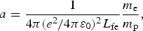 $$a = \displaystyle{1 \over {{\rm 4\pi (}{e^{\rm 2}}/4{\rm \pi} {{\rm \varepsilon} _{\rm 0}}{)^2}{L_{{\rm fe}}}}}\displaystyle{{{m_{\rm e}}} \over {{m_{\rm p}}}},$$
where E p0 and E p1 are energies of the injected and the escaped protons, respectively. A remarkable feature of Eq. (2) is that, assuming E p0 and E p1 are given, the expression contains only one unknown quantity n fe, which can be calculated directly.
When the probing proton beam propagates in the inhomogeneous plasmas in a specific direction, the equation of the densities of grids is
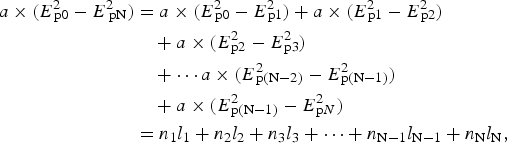 $$\eqalign{a \times ({E^2}_{{\hskip-4pt\rm p}0} - {E^2}_{\,{\hskip-4pt\rm p}{\rm N}} ) & = a \times ({E^2}_{{\hskip-4pt\rm p}0} - {E^2}_{{\hskip-4pt\rm p}1} ) + a \times ({E^2}_{{\hskip-4pt\rm p}1} - {E^2}_{\hskip-4pt{\rm p}2} ) \cr & \quad + a \times ({E^2}_{\hskip-4pt{\rm p}2} - {E^2}_{\hskip-4pt{\rm p}3} ) \cr &\quad + \cdots a \times ({E^2}_{\hskip-4pt{\rm p}({\rm N} - 2)} - {E^2}_{\hskip-4pt{\rm p}({\rm N} - 1)} ) \cr & \quad + a \times ({E^2}_{\hskip-4pt{\rm p}({\rm N} - 1)} - {E^2}_{\hskip-4pt{\rm p}N} ) \cr & = {n_1}{l_1} + {n_2}{l_2} + {n_3}{l_3} + \cdots + {n_{{\rm N} - {\rm 1}}}{l_{{\rm N} - {\rm 1}}} + {n_{\rm N}}{l_{\rm N}},} $$
l 1, l 2, l 3, … l N−1,l N are the distances of this proton beam propagating in each grid, n 1, n 2, n 3, …n N−1, n N are the densities of each grid, respectively.
3. TIKHONOV’ REGULARIZATION METHODS SOLVING THE ILL-POSED EQUATION SET
In order to reveal the density distribution, M (M ≥ N) linear equations of the densities of each grid should be known, which requires M sets of the initial and the final protons energies. Then the following large linear equation set will be obtained,
 $${\bf A}x = b{\rm,} $$
with
 $$\eqalign{{\bf A} & = \left( {\matrix{ {{l_{11}}} & {{l_{1{\kern 1pt} 2}}} & {{l_{1{\kern 1pt} 3}}} & \cdots & {{l_{1{\rm N}}}} \cr {{l_{21}}} & {{l_{2{\kern 1pt} 2}}} & {{l_{23}}} & \cdots & {{l_{{\rm 2 N}}}} \cr {{l_{31}}} & {{l_{32}}} & {{l_{33}}} & \cdots & {{l_{{\rm 3 N}}}} \cr \cdots & \cdots & \cdots & \cdots & \cdots \cr {{l_{{\rm M}1}}} & {{l_{{\rm M}2}}} & {{l_{{\rm M}3}}} & \cdots & {{l_{{\rm M N}}}} \cr}} \right),\quad x = \left( {\matrix{ {{n_1}} \cr {{n_2}} \cr {{n_3}} \cr \vdots \cr {{n_{\rm N}}} \cr}} \right)\,\,{\rm and}\,\, \cr b = &\, a \times \Delta {E^2} = a \times \left( {\matrix{ {{E^2}_{10} - {E^2}_{1{\rm N}}} \cr {{E^2}_{20} - {E^2}_{2{\rm N}}} \cr {{E^2}_{30} - {E^2}_{3{\rm N}}} \cr \vdots \cr {{E^2}_{{\rm M}0} - {E^2}_{{\rm MN}}} \cr}} \right)} $$
The length matrix A can be calculated if the initial position, the propagating direction of proton beams, and the probed area can be known. Unfortunately, the equation set (5) is ill-posed since the matrix A has a very large condition number. Therefore, it is not easy to reveal accurate plasma density with the use of this equation set, even quite accurate final proton energies are measured. In order to reveal accurately the density distribution by solving Eq. (5), the Tikhonov regularization method which is very popular in other similar inverse problems can be applied (Xiao et al., Reference Xiao, Yu, Wang, Shi and Li2003). Here we have to solve λ for the minimized question,
 $$\min \left\{ { \vert \vert {\bf A}x - b \vert { \vert _2}^2 + {{\rm \lambda} ^2}{{\rm I}^{\rm 2}}} \right\},$$
where A T is the transpose of the matrix A, λ is regularization factor, I is the unit matrix. Then, x can be calculated from the equation set below:
 $$({A^{\rm T}}{\bf A} + {\rm \lambda} {{\rm I}^{\rm 2}})x = {A^{\rm T}}b.$$
The way of finding the right regularization factor λ is the fast algorithm based on the principle of L-curve. The error of revealing can be described as (Xiao et al., Reference Xiao, Yu, Wang, Shi and Li2003)
 $$Er{\rm \,= norm(}{\bf D}{\rm ^{\prime} -} {\bf D}{\rm )/norm(}{\bf D}{\rm ),}$$
where D is simulated density matrix and D′ is the revealed density matrix though Tikhonov regularization method.
4. NUMERICAL SIMULATIONS
4.1. The Set Plan for the Numerical Simulation
The 3D dense plasma considered has the density order of 1025/cm3. The x, y, and z coordinates of the zone studied are all between 0 and 210 µm in our coordinate system. The density distribution studied has the expression
 $$n = \left\{ {\matrix{ {{\rm 1}{{\rm 0}^{{\rm 25}}}{\rm /c}{{\rm m}^{\rm 3}} \times {\rm exp(}{\rm -} k{\rm /36)}} & {k \lt 60} \cr 0 & {k \ge 60} \cr}} \right.,$$
where k is the distance between the position and the center of the area (105, 105, 105). The plasma densities of each grid are described as the density at the center of each grid. With this way, a simulated density matrix D of 2744 elements is obtained.
Six identical proton sources are placed at (−180, −150, −390), (105, 105, 390), (−390, −150, −120), (390, 150, 120), (−270, −390, −240), and (240, 390, 210), respectively, with the quasi-monoenergy of 15 MeV. The reason for choosing this energy is described as follows. If the energy is too big, the differences of final energies of different proton beams after propagating through the plasmas are too small to be measured; if the proton energy is too small, the energy of proton beams have already been vanished inside the plasmas. If energy distribution of the laser-generated proton beam is exponential, then the protons with different velocity will reach the plasma zone at different time and after passing though the plasma zone they can be also measured at different time. Therefore, density distributions at different time can be diagnosed and the ultrafast density evolution of the plasmas can be obtained through the exponential energy distribution of the proton beams. The emitting angle of proton sources is about 40° in order that the whole studied zone has been passed through by proton beams. If the emitting angle decreases, the distance from the proton sources to the zone should increase. The energy detectors facing the six proton sources are around 1 mm away from probed area. The matrix A in this simulation has a condition number of the order of 1015, so the equation set (5) is quite ill-posed.
4.2. The Calculation for the Density Distribution
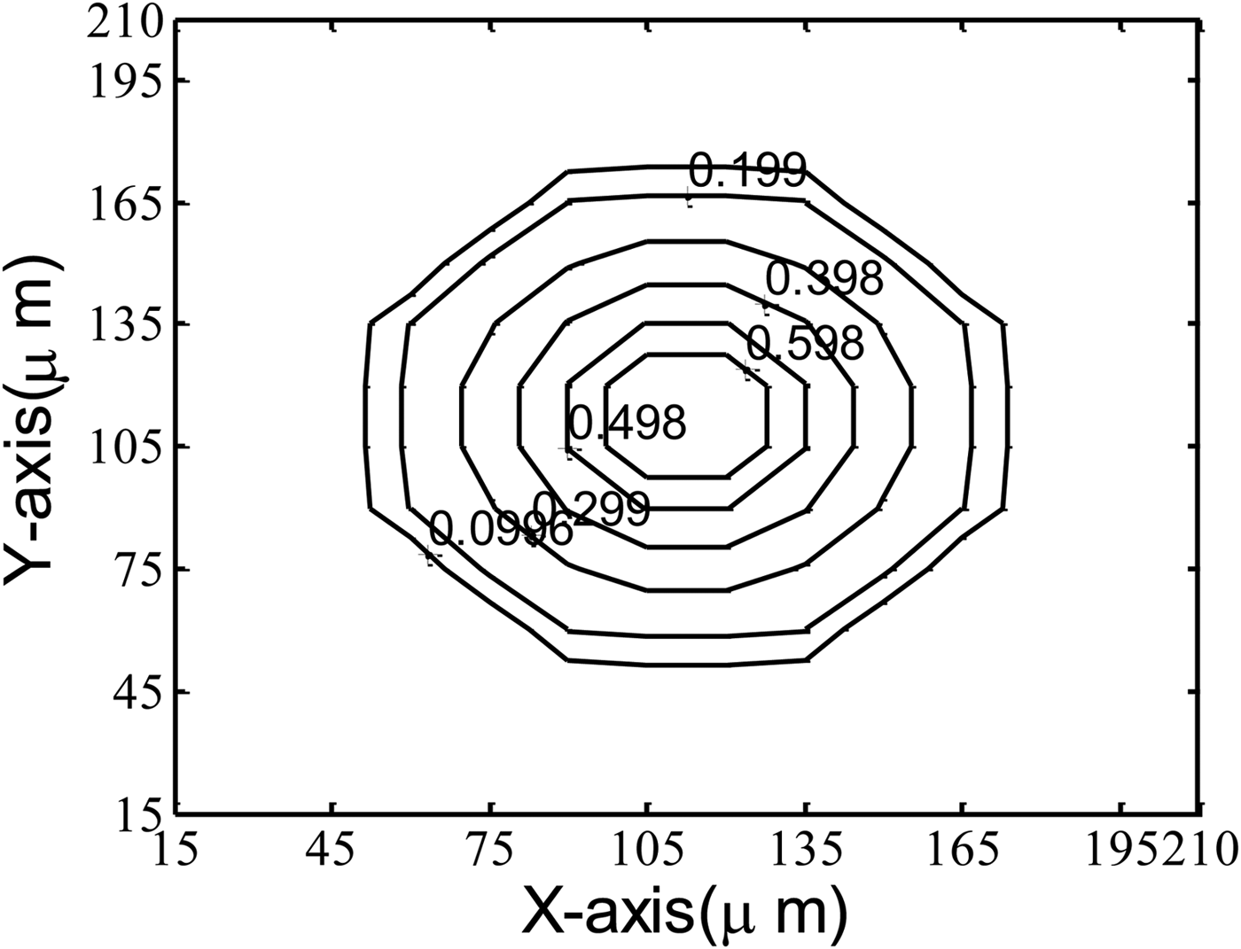
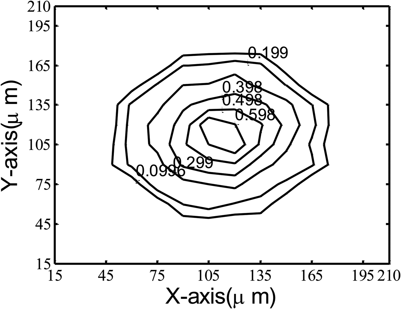
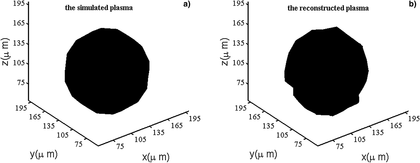
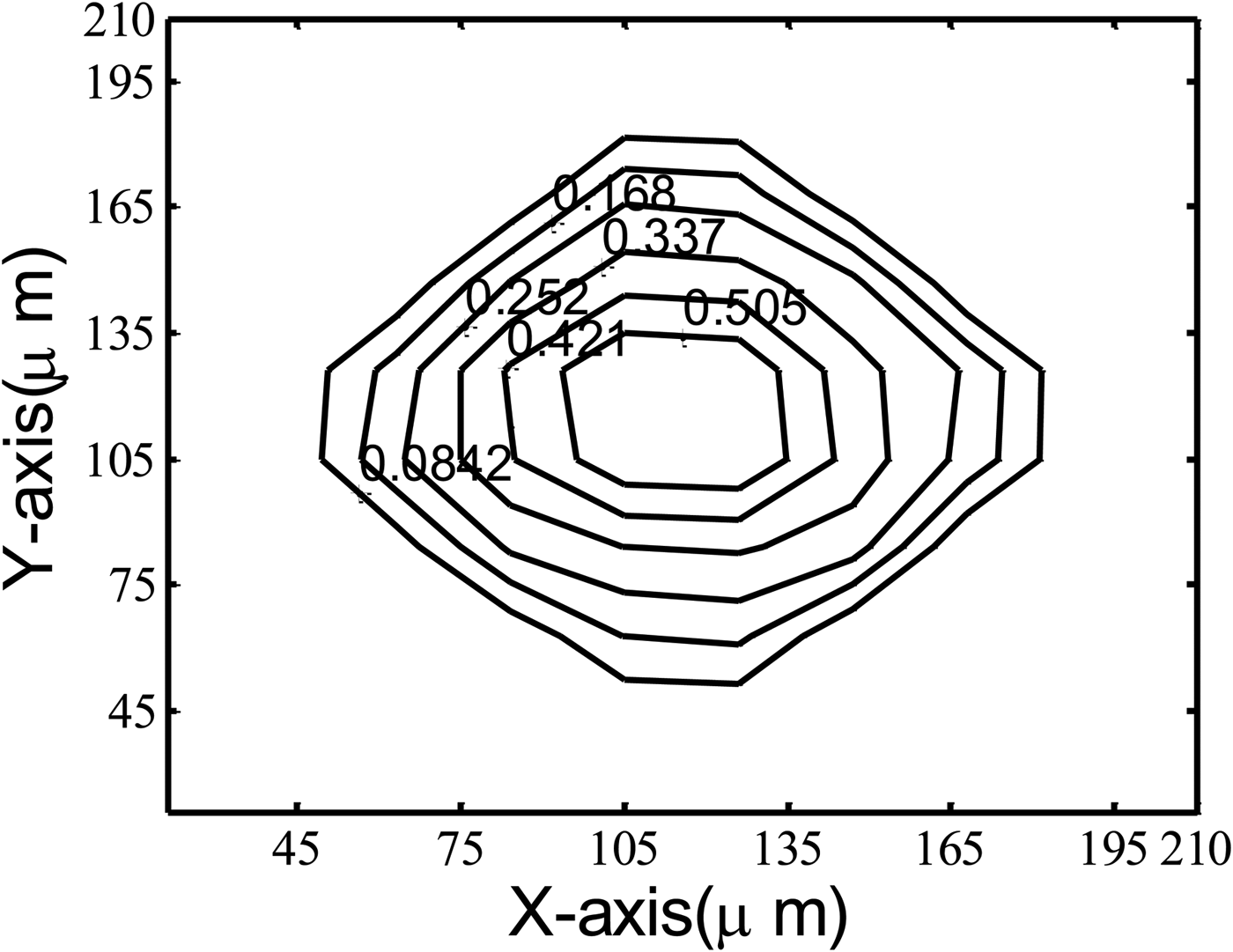
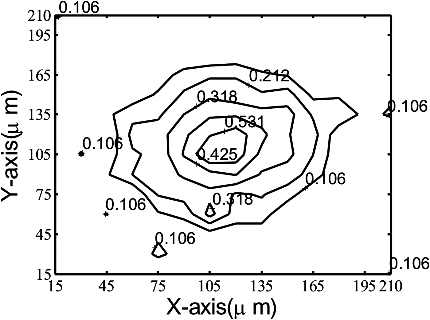
The final energies of each proton beam in specific directions are calculated analytically using Eqs. (1) and (9) for the simulated plasma density, so that an energy matrix of M = 3464 elements is given. With this vector and matrix A, using the Tikhonov regularization method, the revealed density matrix D′ of 2744 elements is obtained and the simulated density profile can be repeated to some degree. The error of 2D reconstruction using four proton sources is 21%. However, the error of 3D reconstruction using four proton sources is 46%, higher than that of 2D reconstruction, which is mainly attributed to the larger reconstruction area and calculation quantity. In order to decrease the errors, the number of proton sources is increased to five, six, and seven, respectively, and the errors are 38, 17, and 16% correspondingly. When more proton sources are used, the experiment will be more difficult, although the accuracy of revealing will be improved. Since the errors of six and seven proton sources are almost the same, six proton sources will be used in this paper. The set plan of six proton sources has been described in the previous section and the error of six proton sources is 17%, which is similar to that of 2D reconstruction with four proton sources. The contour lines of the simulated density D are shown in Figure 1, also the contour lines of the revealed density D′ are shown in Figure 2. Comparing the two figures, we can find that Figure 2 can reflect the correct density distribution. In the zone where the simulated plasmas appear, the revealed density is a little smaller than the simulated one and on the same order of 1025/cm3. As shown in Figure 3, the isopycnic surface comparison between simulated plasma and revealed plasma shows that the revealed density is almost the same as the simulated one except little edge in few areas. Because the density distribution in particular face can reflect simulated density more clearly than isopycnic surface, we will only concentrate on the density distribution in particular face in the following.
The contour lines of the density of the simulated density distribution (z = 105 µm). (The density values are the product of the value of each contour line and 1025/cm3, and this will apply to the figures in the following).

The contour lines of the revealed density without noise (z = 105 µm), the error is described as Er = 17%.
The comparison of isopycnic surface of density 0.2 between simulated and reconstructed plasmas.
4.3. The Comparisons among Different Picture Elements
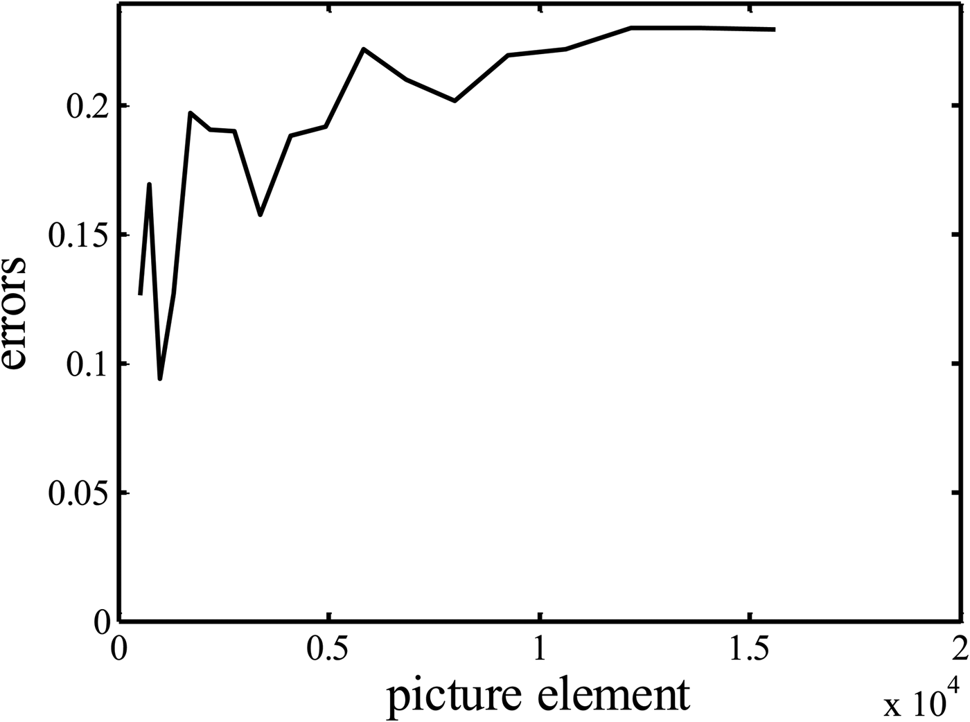
Different picture elements can obtain different errors in the reconstruction simulations. The reconstructions of different picture elements of 512 (N = 83), 729 (N = 93), 1000 (N = 103), 1331 (N = 113), 1728 (N = 123), 2197 (N = 133), 2744 (N = 143), 3375 (N = 153), 4096 (N = 163), 4913 (N = 173), 5832 (N = 183), 6859 (N = 193), 8000 (N = 203), 9261 (N = 213), 10,648 (N = 223), 12,167 (N = 233), 13,824 (N = 243), and 15,625 (N = 253) are simulated, respectively. The corresponding errors are shown in Figure 4. The smallest error appears when the picture element is 1000 (N = 103). Then the errors increase to certain level until the picture element is 2744 (N = 143) and then decrease when the picture element is 3375 (N = 153). In the following, the errors will increase again as the picture elements increase until the picture elements is 5832 (N = 183). Then the errors remain stable around 23% for the following larger picture elements. When the picture element is 1000, the error is smallest as 10% but the reconstructed density is not similar to the simulated density. As shown in Figure 5, the corresponding contour lines of the revealed density are not smooth as circles while the contour lines of the simulated density are circular. When the picture element is 3375, the error is a little smaller than that of 2744 element as 16% but special computers with much bigger memory are required, which is not convenient for the ordinary calculation. In summary, if the picture element is too small, the reconstructed density cannot reveal the simulated density well; if the picture element is too big, the calculation time and scale are too big to be processed by ordinary computers. Therefore, the picture element is chosen as 2744 in this paper.
The errors of different picture elements.
The contour lines of the revealed density for picture element of 1000. The error is described as Er = 9%.
Generally speaking, as shown in Figure 4, the errors increase at first and then remain stable after certain picture element (5832). Calculation amounts increase with the increase of the picture elements, so the errors increase when the picture elements increase from 83 to 183. However, the errors remain stable when picture elements are larger than one certain picture element of 193, which is mainly attributed to the enough density sample points for these numerical simulations. The simulated zone has been divided into grids small enough when picture elements are larger than 193, so the errors do not change when picture elements increase from 193 to 253, which is very common in the numerical simulation. The errors will not change much when the numbers of the sample points exceed one certain value. As for the smaller elements (83, 93, 103, 113), the errors do not always increase as the picture elements increase, which are mainly attributed to the insufficient density sample points for the simulated plasmas.
4.4. The Comparison between Tikhonov Regularization Method and SIRT Method
We can finish one calculation in 10 min using the fast Tikhonov regularization method and the error of 3D reconstruction is at the same level of 2D reconstruction. The calculation time depends mainly on CPU and memory of the computer. The CPU of our computer has four Intel cores and the frequency of these cores is 3.40 GHz. The memory capacity of our computer is 4G. We also have done the reconstruction with SIRT method which requires 12 h using the same relaxing factor (3.3163 × 10⁻⁴) as the 2D reconstruction and the error is 49%. Generally speaking, small relaxing factors increase the calculation accuracy at the cost of calculation time. However, the error of SIRT with the small relaxing factor as 3.3163 × 10⁻⁴ is still higher than that of the Tikhonov regularization method. Judging from the calculation time and accuracy, the Tikhonov regularization method can calculate faster with smaller error than that of SIRT method. Therefore, we choose the Tikhonov regularization method for the 3D density reconstruction in this paper.
4.5. The Effect of Noises on the Reconstruction Errors
Radio-Chromic Film is one kind of energy detectors and has been used for high-flux proton detection in several laser–plasma experiments. The uncertainty of the measurement is no more than 5% (McLaughlin et al., Reference Mclaughlin, Chen, Soares, Miller, Van Dyk and Lewis1991), and can even decrease to 2% in some measurements (Nichiporov et al., Reference Nichiporov, Kostjuchenko, Puhl, Bensen, Desrosiers, Dich, Mclaughlin, Kojima, Coursey and Zink1995; Christopher, Reference Christopher2007). So we add two kinds of noises to the final proton energies:
 $$\eqalign{E{{\rm ^{\prime}}_{{\rm final}}} & = {E_{{\rm final}}} \times (1 - 0.02 \times {\rm rand}({\rm size}({E_{{\rm final}}}))), \cr & E{{\rm ^{\prime}}_{{\rm final}}} = {E_{{\rm final}}} \times (1 - 0.05 \times {\rm rand}({\rm size}({E_{{\rm final}}}))).} $$
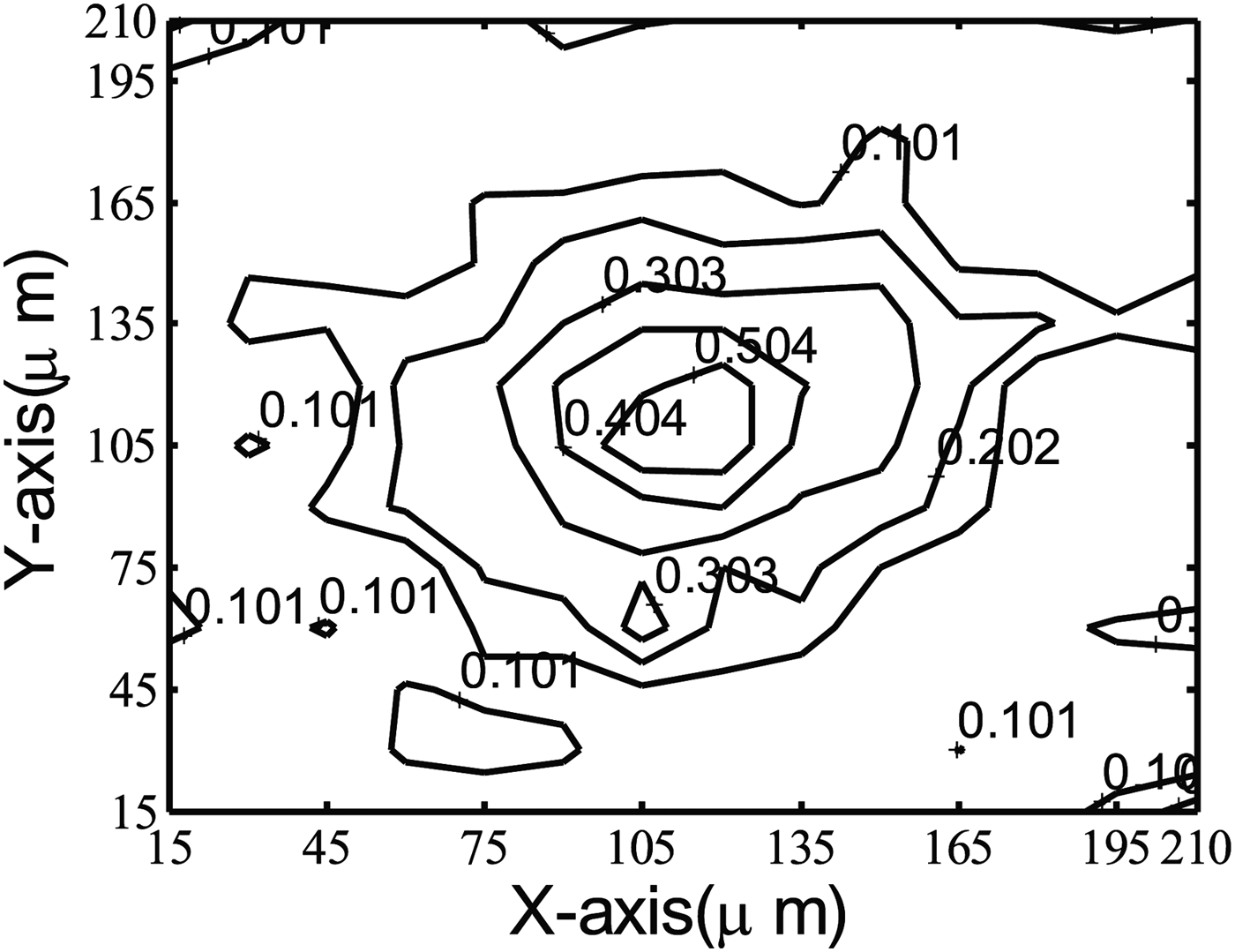
The corresponding revealing errors are 30 and 44%, also the contour lines of calculated densities are shown in Figures 6 and 7, respectively.
The contour lines of the revealed density distribution (z = 105 µm) with noises level of 2% added to the final proton energies. The error of revealing is described as Er = 30%.
The contour lines of the revealed density distribution (z = 105 µm) with noises level of 5% added to the final proton energies. The error of revealing is described as Er = 44%.
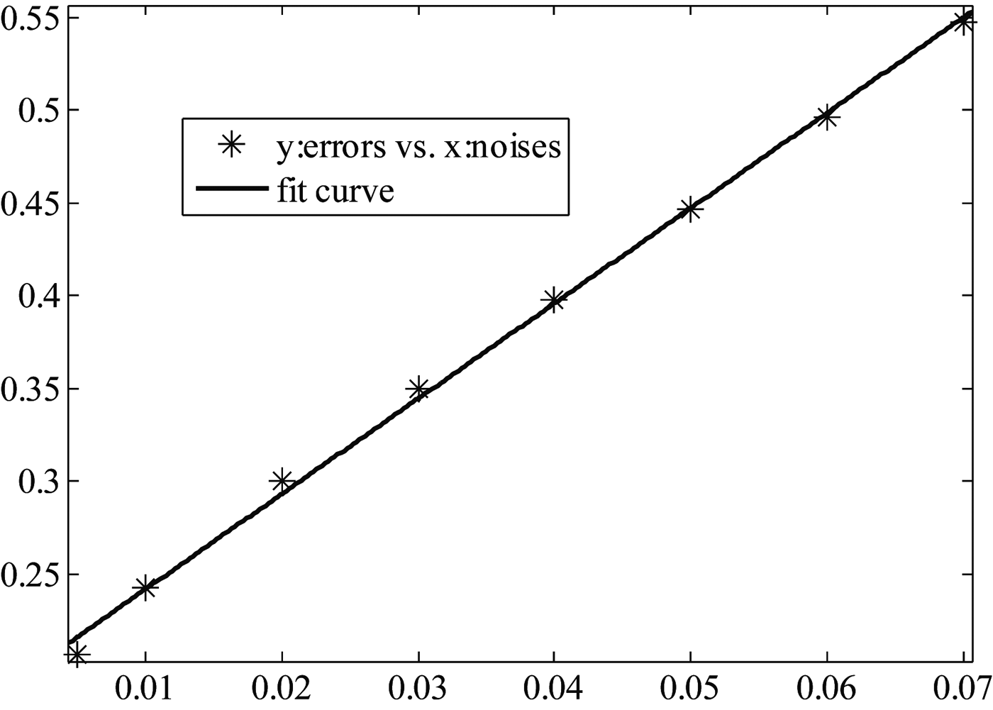
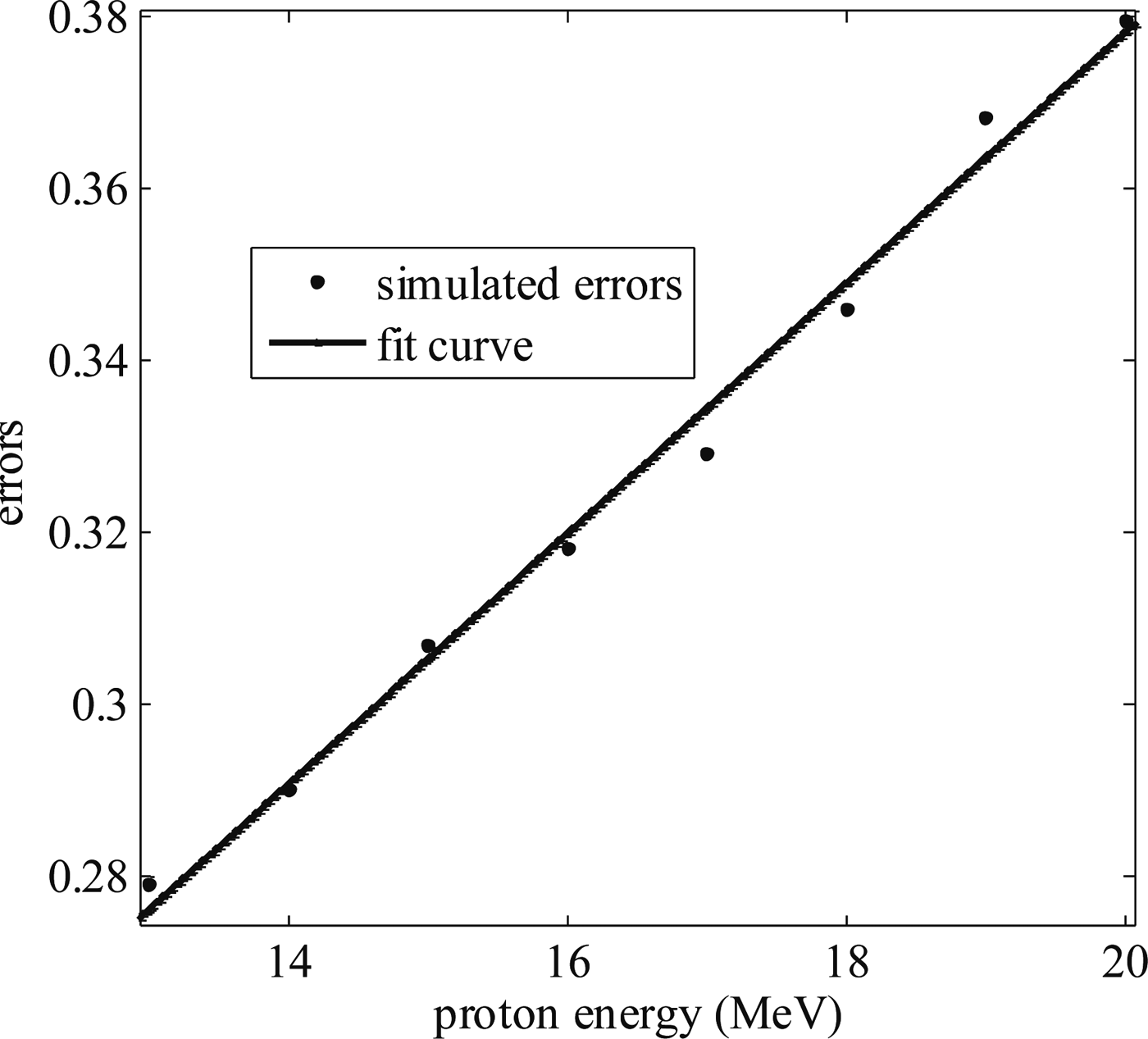
Furthermore, a relation between the errors and the noises are established. An analytical expression between them through fifth degree polynomial fit is obtained as f(x) = p 1 × x + p 2. The coefficients are p 1 = 5.134, p 2 = 0.1905, respectively, and the R-square is 0.9981, which proves the high accuracy of this fitness. The corresponding scatter diagram and the fit curve are shown in Figure 8, which shows that they are in good agreement.
The scatter diagram and the fit curve between the noises and corresponding errors.
For the 2D reconstruction, the density reconstruction is also done without and with two kinds of noises (2 and 5%) to the final proton energies and the revealing errors are 20, 26, and 37%, respectively. Comparing the results of 3D reconstruction with those of 2D reconstruction, it shows that the effects of noises on the 3D reconstruction errors are higher than that of 2D reconstruction. However, the contour lines of calculated densities are capable of revealing the simulated densities as shown in Figures 6 and 7, except at the points where the simulated plasmas do not appear. In the zone where the simulated plasmas appear, the density revealed is a little smaller than the simulated one and on the same order of 1025/cm3. In the zones where the simulated plasmas do not appear, the revealed density appears in some of these zones, which is the one reason for the high effect of the noises on the 3D reconstruction errors. In our opinion, the high effects of the noises on the errors are mainly attributed to the appearance of plasmas where there are no plasmas in the simulated zone and the large calculation quantity of 3D reconstructions.
In order to prove the reason for the high effects of the noises on the errors, two other different plasma density distributions are simulated. One density distribution studied has the expression
 $$n = \left\{ {\matrix{ {{\rm 1}{{\rm 0}^{{\rm 25}}}{\rm /c}{{\rm m}^{\rm 3}} \times {\rm exp(}{\rm -} k{\rm /36)}} & {k \lt 140} \cr 0 & {k \ge 140} \cr}} \right.,$$
where k is the distance between the position and the center of the area (105, 105, 105). In this way, a simulated density matrix D of 2744 elements is obtained and none of the matrix element is zero implying that plasmas appear everywhere in the simulated zone. The errors are 10 and 25% with no noise and with 2% noises added to the final protons energies, respectively, which are both smaller than the errors of the simulated plasmas distributions represented with Eq. (9). Therefore, if the borders of the plasma region are roughly determined before the density reconstruction and the density of each grid in the simulation in not zero, the reconstruction errors from the energy noises can be decreased. Furthermore, the effects of density gradient on the reconstruction errors are also studied through the density reconstruction of homogeneous plasmas with the density 0.2 × 1025/cm3. Through simulation, the errors of simulation without errors and with 2% noises added to the final energies are 3 and 20%, respectively. Therefore, the simulation errors will be increased for density distribution with significant density gradient while errors will be decreased for those with small density gradient.
4.6. The Effect of Proton Sources on the Reconstruction Errors
In our above calculation, six identical proton sources are placed at (−180, −150, −390), (105, 105, 390), (−390, −150, −120), (390, 150, 120), (−270, −390, −240), and (240, 390, 210), respectively. In order to study the effect of the proton sources arrangements on the reconstruction accuracy, different proton sources arrangements are chosen. Through these different simulation experiments, the best points obtained are (0, 0, −390), (105, 105, −390), (−390, 105, 105), (90, −390, 90), (390, 150, 150), and (90, 390, 120) with the error of 10% when no noises are added to the final proton energy. Comparing the two listed arrangements of proton sources, the following conclusion can be obtained. In order to obtain energy information in the whole simulated plasma and increase the reconstruction accuracy, the proton sources should spread around the simulated plasma zone as much as possible.
If the differences of final energies of different proton beams after propagating through the plasmas are too small, it indicates that the incident proton energy is too big. If the energy of proton beams has already been vanished inside the plasmas, it indicates the incident proton energy is too small. Therefore, acceptable energies of the incident proton beam can be chosen according to these principles. In order to study the effect of these acceptable incident energies of quasi-monoenergetic proton beams on the reconstruction accuracy, simulations of different initial proton energies are done in this paper. As shown in Figure 9, the effects of initial proton energies on the reconstruction errors are not big and the errors increase slightly with the increase of the incident proton energies. As mentioned above, density distributions at different time can be diagnosed and the ultrafast density evolution of the plasmas can be obtained through the exponential energy distribution of the proton beams.
The effect of initial proton energy on the reconstruction errors with noises level of 2% added to the final proton energies.
5. CONCLUSION
Particular properties of the protons generated in the laser–plasma interaction have made them suitable for the diagnostic of dense plasmas. Our diagnostics of the density distribution of the inhomogeneous plasma is most suitable for dense and thick plasmas, especially in the case of laser fusion. From the Coulomb energy loss of protons propagating in the inhomogeneous plasmas, we obtain a large linear and ill-posed equation set of each grid density, solved by the Tikhonov regularization method which is very popular in other inverse problems. The 3D density distribution can be obtained using six proton sources and the error is at the same level of that of 2D reconstruction. The picture element N is chosen as 2744 with consideration of smoothness and calculation memory of the computers. The revealing errors are 17, 30, and 44% without and with two kinds of noises (2 and 5%) to the final proton energies and an analytical relation between the errors and the noises are established in this paper. If the borders of the plasma region are roughly determined before the density reconstruction, the reconstruction errors from the energy noises can be decreased. The speed of Tikhonov regularization method is faster than the SIRT method with smaller errors. Therefore, 3D density reconstructions are done using Tikhonov regularization method in this paper. In order to obtain energy information in the whole simulated plasma and increase the reconstruction accuracy, the proton sources should spread around the simulated plasma zone as much as possible. The effects of initial proton energies on the reconstruction errors are not big and the errors increase slightly with the increase of the incident proton energies.
ACKNOWLEDGMENT
This research was supported by Zhejiang Provincial Natural Science Foundation of China under Grant No. LQ16A050001 and the Scientific Research Fund for Talented Scholars, Zhejiang Ocean University (23025010113).