





1. Introduction
Quantitative understanding of heat and mass transport in heterogeneous porous media remains a fundamental challenge across numerous scientific and engineering disciplines. Applications as diverse as the use of heat as tracer to characterise heterogeneous (including fractured) subsurface media (Silliman & Robinson Reference Silliman and Robinson1989; Klepikova et al. Reference Klepikova, Le Borgne, Bour and Davy2011), thermal remediation of polluted soils (Hinchee & Smith Reference Hinchee and Smith1992), geothermal energy (Shaik et al. Reference Shaik, Rahman, Tran and Tran2011) and blood perfusion (Pennes Reference Pennes1948) all involve intricate interactions between advective transport through high-permeability pathways and diffusive exchange with surrounding low-permeability matrices. These systems are typically characterised by structural heterogeneity spanning many orders of magnitude in scale, resulting in strongly non-Fickian behaviour, e.g. long-tailed residence time distributions (Roubinet, de Dreuzy & Tartakovsky Reference Roubinet, de Dreuzy and Tartakovsky2013).
The exchange between mobile and immobile zones in porous media, e.g. fractures and matrix and/or preferential flow paths and stagnant domains, controls large-scale transport efficiency, long-term retention and the evolution of reactive processes (Yang & Tartakovsky Reference Yang and Tartakovsky2025 and references therein). Development of robust modelling frameworks that accurately capture these multiscale, flow-driven exchange mechanisms is essential for predictive analysis, risk assessment and optimal design in a plethora of applications. In the case of heat transport, this exchange corresponds to conductive heat transfer from fractures into the surrounding rock matrix and heat transport within that matrix.
The present work addresses coupled flow and heat transport in fractured geological formations, which are a good framework to illustrate the modelling challenges. Subsurface environments are often composed of a low-permeability porous matrix (granite, shale, metamorphic rock, etc.), with intrinsic permeability typically in the
 $10^{-20}$
–
 $10^{-16}\,\textrm{m}^2$
range. The matrix contains a network of interconnected fractures with local permeability as high as
 $10^{-10}\,\textrm{m}^2$
, depending on fracture aperture, spacing, orientation distribution and degree of connectivity (Bonnet et al. Reference Bonnet, Bour, Odling, Davy, Main, Cowie and Berkowitz2001; Viswanathan et al. Reference Viswanathan2022). This contrast in hydraulic properties restricts fluid flow to the fractures, while heat transport in the surrounding matrix is dominated by heat conduction.
Fracture–matrix interactions control the partitioning of heat between mobile and immobile domains, and therefore, the degree to which the surrounding rock participates in thermal storage (Ruiz Martinez, Roubinet & Tartakovsky Reference Ruiz Martinez, Roubinet and Tartakovsky2014 and references therein). Even modest geometric variability within a single fracture can reorganise the flow into preferential channels and low-velocity pockets, producing sharp thermal fronts and spatially uneven heat uptake (Gisladottir, Roubinet & Tartakovsky Reference Gisladottir, Roubinet and Tartakovsky2016). Numerical analyses of heat transfer in discrete-fracture networks (e.g. Geiger & Emmanuel Reference Geiger and Emmanuel2010) and in explicitly resolved rough-walled single fractures (e.g. Klepikova et al. Reference Klepikova, Méheust, Roques and Linde2021) show that structural heterogeneity, arising respectively from network connectivity or from aperture variability, organises the flow into preferential channels and regions of quasi-immobile flow. These heterogeneous flow patterns enhance advective intermittency and promote repeated equilibration with the surrounding rock matrix, thereby exerting a strong control on the timing of thermal breakthrough, thermal recovery and overall heat extraction efficiency.
Field-scale thermal tracer tests (Klepikova et al. Reference Klepikova, Le Borgne, Bour, Dentz, Hochreutener and Lavenant2016; de La Bernardie et al. Reference de La Bernardie, Bour, Le Borgne, Guihéneuf, Chatton, Labasque, Le Lay and Gerard2018) exhibit analogous behaviour: early breakthrough, a gradual intermediate decline and tails, consistent with the combined effects of channelised flow, matrix conduction and intermittent trapping. Together, these observations demonstrate that realistic fracture geometries govern the large-scale thermal response of fractured media and motivate modelling strategies that explicitly resolve aperture variability rather than relying on homogenised representations.
Furthermore, at the fracture scale, geological fracture walls exhibit self-affine roughness (Schmittbuhl et al. Reference Schmittbuhl, Schmitt and Scholz1995a ) and are unmatched below a characteristic correlation length (Brown Reference Brown1995). This generates heterogeneous aperture fields containing nearly closed zones as well as spatially correlated large-aperture channels extending up to the scale of the correlation length. The resulting flow patterns are strongly channelised, with channelling intensity all the larger as the fracture is more closed (i.e. as aperture heterogeneity is larger (Brown Reference Brown1987; Méheust & Schmittbuhl Reference Méheust and Schmittbuhl2001a )), and with preferential flow-channel sizes (as well as low permeability region sizes) limited by the underlying correlation scale (Méheust & Schmittbuhl Reference Méheust and Schmittbuhl2003; Lenci et al. Reference Lenci, Putti, Di Federico and Méheust2022b ). Consequently, fracture flow can deviate markedly from parallel-plate predictions based solely on the mean aperture.
This geometric variability dictates thermal breakthrough behaviour through its control on the competition between advective transport along preferential channels and diffusive exchange in low-velocity pockets (Neuville, Toussaint & Schmittbuhl Reference Neuville, Toussaint and Schmittbuhl2010; Klepikova et al. Reference Klepikova, Méheust, Roques and Linde2021). Across both network and single-fracture scales, the coexistence of preferential conduits and quasi-immobile zones causes transport to alternate between advection- and diffusion-dominated regimes, producing strong spatial intermittency. Efficiently capturing this behaviour requires mesh-free particle-based methods capable of resolving the broad spectrum of residence times induced by roughness-controlled channelling.
We present here a hybrid stochastic–physical model for heat transfer in a fracture–matrix system, which accounts for both heat advection within fractures and heat conduction in the fluid, and exchange of heat with a heat-conducting matrix. Heat advection and conduction in the flowing fluid are modelled with a time-domain random walk (TDRW) scheme (Delay & Bodin Reference Delay and Bodin2001; Russian, Dentz & Gouze Reference Russian, Dentz and Gouze2016), i.e. heat particle trajectories in the fracture evolve through random time increments, while spatial displacements are dictated by the local depth-averaged velocity. This framework efficiently captures the strong velocity contrasts of rough fractures: particles propagate rapidly along high-velocity channels and remain effectively immobilised in nearly closed regions, without requiring prohibitively small time steps or finely resolved grids (Noetinger et al. Reference Noetinger, Roubinet, Russian, Le Borgne, Delay, Dentz, de Dreuzy and Gouze2016). The fracture–matrix exchange is modelled by an analytically derived kernel: the matrix residence-time distribution is obtained directly from the Green’s function of transient one-dimensional conduction, yielding a calibration-free and thermodynamically consistent description of conductive heat loss from the fracture. Stochastic propagation is performed over explicitly resolved rough-walled geometries so that aperture-controlled heterogeneity directly determines both advective residence times and local exchange histories. We thus obtain a predictive and computationally efficient representation of non-Fickian thermal transport that retains the full imprint of the heat transport processes at play.
The model is validated against analytical solutions and high-fidelity finite-element simulations. To systematically assess the influence of heterogeneity and flow conditions, we conduct a Monte Carlo (MC) analysis over multiple combinations of relative fracture closure, spatial correlation length and Péclet number, thereby encompassing a broad range of geologically plausible scenarios. Results are presented in terms of four key observables: mean longitudinal displacement, displacement variance, breakthrough curves and heat-exchange efficiency at the fracture–matrix interface. These quantities allow the distinction among transport regimes (ballistic, diffusive, subdiffusive), characterise the spreading of the thermal front and quantify the efficiency of heat extraction over time. Their temporal evolution provides a concise macroscopic signature of how advective and conductive mechanisms jointly shape heat transport in rough-walled fractures, complementing the process-level understanding derived from the underlying stochastic model.
The manuscript is organised as follows. Section 2 introduces the geometrical characterisation of the fracture aperture field and the generation of synthetic rough-walled fractures. Section 3 presents the depth-averaged flow model based on the lubrication approximation, and § 4 details the TDRW formulation coupled with the semi-analytical fracture–matrix heat-exchange model. Validation against analytical solutions and finite-element simulations is provided in § 5. Section 6 examines the statistical behaviour of heat transport across varying heterogeneity levels and Péclet numbers, including displacement moments, breakthrough curves and heat exchange efficiency. Conclusions and perspectives are summarised in § 7. Appendix A derives the matrix trapping-time distribution, Appendix B presents the associated memory kernel and Appendix C outlines numerical implementation aspects.
2. Synthetic geological fractures
Geological fractures are discontinuities in the rock matrix, which arise from fracturing in the material due to tectonic or thermal constraints and which are quasi-planar at large scales. They are inherently heterogeneous. Laboratory and field measurements show that the roughness of both synthetic (Schmittbuhl et al. Reference Schmittbuhl, Schmitt and Scholz1995b
) and natural (Renard, Candela & Bouchaud Reference Renard, Candela and Bouchaud2013) fracture surfaces displays self-affine scale-invariance over several orders of magnitude. When data obtained from different measurement techniques and surfaces of different sizes are combined, the scaling extends over 7–12 decades, from the smallest resolved laboratory scales up to the dimensions of large faults (Candela et al. Reference Candela, Renard, Bouchon, Brouste, Marsan, Schmittbuhl and Voisin2009). This self-affinity means that the surfaces are statistically invariant by any rescaling of the in-plane coordinates by any factor
 $\lambda$
, provided that the out-of-plane coordinate is rescaled by
 $\lambda ^H$
, the so-called Hurst exponent being primarily characteristic of the fracturing process. The value of this exponent is independent of rock type (and even of brittle material type) or geologic and tectonic environments (Bouchaud, Lapasset & Plane Reference Bouchaud, Lapasset and Plane1990; Renard et al. Reference Renard, Candela and Bouchaud2013; Milanese et al. Reference Milanese, Brink, Aghababaei and Molinari2019). An exception arises in sandstones, where intergranular fracturing sets the lower scale for self-affinity to the grain scale and induces a lower Hurst exponent, with
 $H \approx 0.45$
(Boffa et al. Reference Boffa, Allain, Chertcoff, Hulin, Plouraboue and Roux1999). Measurements on exposed fault surfaces indicate the combined action of brittle failure and plastic deformation, and three-body wear leads to a universal smoothing process (Sagy, Brodsky & Axen Reference Sagy, Brodsky and Axen2007), which may alter the roughness amplitude in time (in particular, as a consequence of fault slip), but conserves the surfaces’ self-affinity. However, recent numerical results show that self-affine walls may also develop from initially flat surfaces due to three-body wear over large times (Milanese et al. Reference Milanese, Brink, Aghababaei and Molinari2019). In Fourier space, the self-affine scale-invariance of the fracture walls is reflected in a power-law decay of the power spectral density (PSD) of their topographies,
 \begin{equation} {\mathcal{F}}({\kappa})\,\, {\propto}\,\, {\kappa}^{-(2+2H)}, \end{equation}
which holds for wavenumbers
 $\kappa$
between cutoffs associated with the aforementioned characteristic scales. The wavenumber provides a natural indexing of the spatial scales of the roughness: modes with small
 $\kappa$
correspond to large-scale aperture variations, whereas modes with large
 $\kappa$
represent fine-scale variations.
(a) Synthetic fracture aperture fields for increasing correlation ratios
 $L / L_{\textit{c}} = \{2,\,16,\,64\}$
(left to right), all with the same fracture closure
 $\sigma _a / \langle a\rangle = 0.8$
. (b) Dimensionless velocity magnitude field,
 $\log _{10}(u/\langle u\rangle )$
, for the case
 $L / L_{\textit{c}} = 16$
, showing the flow structure under the applied boundary conditions. (c) Transverse fracture profile illustrating wall roughness, aperture geometry, matrix domain, and the initial and boundary conditions for flow and transport. Panels (b) and (c) also indicate the transport mechanisms considered in both fracture and matrix. All synthetic aperture fields were generated using
 $L_{\textit{c}} = 0.1\,\textrm {m}$
,
 $H = 0.8$
,
 $a_{\textit{m}} = 1\,\textrm {mm}$
and
 $\sigma _a / \langle a \rangle = 0.8$
.

The separation between the two rough walls of a fracture defines the fracture’s aperture field (figure 1
c). For a horizontal fracture with upper and lower walls of respective topographies
 $x_{3,{u}}$
and
 $x_{3,\textit{l}}$
,
 \begin{equation} a(\boldsymbol{x}) = x_{3,{u}}(\boldsymbol{x}) - x_{3,\textit{l}}(\boldsymbol{x}) + a_{\textit{m}}, \end{equation}
where
 $\boldsymbol{x}=(x_1,x_2)^\top$
is the in-plane position vector and
 $a_{\textit{m}}$
is the mechanical aperture, defined as the distance between the (parallel) mean planes of the opposing walls. Surface features of the two walls tend to match above a characteristic in-plane scale, the correlation length
 $L_{\textit{c}}$
(Brown Reference Brown1995; Méheust & Schmittbuhl Reference Méheust and Schmittbuhl2003). Hence, for wavelengths smaller than
 $L_{\textit{c}}$
(i.e.
 $\kappa \gt 2\pi /L_{\textit{c}}$
), the self-affine wall topographies, which are uncorrelated with each other at these scales, provide the aperture field with the same self-affinity, so that its PSD exhibits the same characteristic power-law behaviour (2.1) (Brown Reference Brown1995). In contrast, at length scales larger than
 $L_{\textit{c}}$
(i.e.
 $\kappa \lt 2\pi /L_{\textit{c}}$
), the PSD flattens. The fracture aperture is thus a spatially heterogeneous random field characterised by its mean aperture
 $\langle a \rangle$
, standard deviation
 $\sigma _a$
, characteristic length
 $L_{\textit{c}}$
controlling the scale range for self-affinity, fracture size
 $L$
setting the domain extent, and Hurst exponent
 $H$
.
Synthetic aperture fields with prescribed statistical properties are generated using fast Fourier transform (FFT)–based spectral synthesis (Méheust & Schmittbuhl Reference Méheust and Schmittbuhl2003; Lenci et al. Reference Lenci, Putti, Di Federico and Méheust2022b
). For a given roughness amplitude
 $\sigma _a$
, the degree of fracture closure is controlled by adjusting the mean aperture
 $\langle a\rangle$
. Where the resulting aperture becomes negative, corresponding to wall–wall contact, the aperture is set to zero, yielding a connected network of flow paths interspersed with impermeable contact zones (Brown Reference Brown1995; Méheust & Schmittbuhl Reference Méheust and Schmittbuhl2001b
). If no contact occurs, the mean aperture coincides with the mechanical aperture,
 $\langle a\rangle = a_{\textit{m}}$
; otherwise, it exceeds it. Representative realisations are shown in figure 1(a) for correlation ratios
 $L/L_{\textit{c}}=\{2,16,64\}$
and fracture closure
 $\sigma_{\textit{a}}/\langle a\rangle =0.8$
.
The aperture fields are generated directly on the computational grid, with the self-affine power spectrum sampled over the range of wavenumbers resolved by the mesh, thereby avoiding interpolation or mesh refinement. Although self-affinity formally implies increasing aperture gradients as the grid spacing decreases, the amplitude of the added high-wavenumber modes simultaneously vanishes, so that mesh refinement does not significantly affect the validity of the lubrication approximation in practice. The grid resolution is therefore chosen to resolve flow structures well below the correlation length while keeping aperture gradients within acceptable lubrication limits over most of the domain. Under this criterion, both the statistical properties of the aperture field, and the resulting hydraulic and thermal responses are insensitive to moderate changes in grid resolution.
Note that the heterogeneity of the aperture field is jointly controlled by the fracture closure ratio,
 $\sigma _a / \langle a\rangle$
, the correlation ratio,
 $L / L_{\textit{c}}$
, and the Hurst exponent. The fracture closure prescribes the relative amplitude of aperture fluctuations with respect to a given mean aperture, thereby setting the overall contrast of the local transmissivity field and controlling, in particular, the probability density function (p.d.f.) of local apertures. The correlation ratio
 $L/L_{\textit{c}}$
determines how many statistically distinct roughness domains are represented within a single realisation. Hence, large
 $L/L_{\textit{c}}$
values correspond to aperture fields composed of many quasi-independent geometric segments, whereas small
 $L/L_{\textit{c}}$
indicates that the geometry is dominated by a few long-wavelength features. Finally, the Hurst exponent
 $H$
specifies the degree of self-affine smoothness of the walls, controlling the relative weight of long- versus short-wavelength asperities in the aperture spectrum.
The thermal properties of water and granite (table 1) are taken from standard datasets (Incropera et al. Reference Incropera, DeWitt, Bergman and Lavine2007) and from measurements in crystalline formations (Klepikova et al. Reference Klepikova, Le Borgne, Bour, Dentz, Hochreutener and Lavenant2016; Kant et al. Reference Kant, Ammann, Rossi, Madonna, Höser and Rudolf von Rohr2017), which ensures consistency with typical hydrothermal conditions. The geometric parameters of the medium (Hurst exponent, correlation ratio and closure ratio) follow the choices justified in § 2 based on documented statistical features of natural self-affine fractures. The numerical aspects related to aperture-field generation, mesh discretisation and solution of the lubrication flow follow the implementation detailed by Lenci et al. (Reference Lenci, Putti, Di Federico and Méheust2022b ).
Physical and numerical parameters defining the fracture geometry, fluid properties and matrix characteristics. All values are fixed across all simulations.

3. Flow in fractures with self-affine walls
Consider the flow of an incompressible fluid, with density
 $\rho _{w}$
and dynamic viscosity
 $\mu _{w}$
, in a horizontal fracture with mechanical aperture
 $a_{\textit{m}}$
. The flow is driven by an imposed pressure gradient
 $\langle \boldsymbol{\nabla }P\rangle$
and is characterised by the Reynolds number,
 \begin{equation} {\textit {Re}} = \frac {\rho _{w} U_{\textit{c}} \ell _{x_3}^2}{\mu _{w}\, \ell _{\boldsymbol{x}}}, \end{equation}
where
 $U_{\textit{c}}$
is a characteristic fluid velocity assumed equal to the maximum velocity within a parallel plate fracture of aperture
 $a_{\textit{m}}$
, that is,
 $u_{\textrm{max}}=a_{\textit{m}}^2\langle \boldsymbol{\nabla }P\rangle /8\mu _{w}$
; and
 $\ell _{x_3} = a_{\textit{m}}$
and
 $\ell _{\boldsymbol{x}} = L_{\textit{c}}$
denote characteristic length scales associated with the vertical and in-plane variations of the velocity field, respectively (Méheust & Schmittbuhl Reference Méheust and Schmittbuhl2001a
; Neuville, Toussaint & Schmittbuhl Reference Neuville, Toussaint and Schmittbuhl2011). Under these conditions, the steady-state fluid velocity
 $\boldsymbol{u}^\prime (\boldsymbol{x}^\prime ) = (u_1, u_2, u_3)^\top$
and pressure
 $p(\boldsymbol{x}^\prime )$
within a fracture
 $\varOmega _{\textit{f}}^\prime = \{ \boldsymbol{x}' = (x_1, x_2, x_3)^\top \in \mathbb{R}^3 : (x_1, x_2) \in (0, L) \times (0, L),\; x_{3,\textit{l}} \leqslant x_3 \leqslant x_{3,{u}} \}$
satisfy the incompressible Stokes equations
 \begin{align} \rho _{w} \boldsymbol{g} - \boldsymbol{\nabla }^\prime p + \mu _{w} \boldsymbol{\nabla }^{\prime 2} \boldsymbol{u}^\prime = \boldsymbol{0}, \qquad \boldsymbol{\nabla }^\prime \boldsymbol{\cdot }\boldsymbol{u}^\prime = 0, \qquad \boldsymbol{x}^\prime \in \Omega _{\textit{f}}^\prime , \end{align}
where
 $\boldsymbol{g} = (0, 0, -g)^\top$
is the gravitational acceleration constant, and the operators
 $\boldsymbol{\nabla }^\prime$
and
 $\boldsymbol{\nabla }^{\prime 2}$
are the gradient and Laplacian in three dimensions.
Randomness of the fracture wall topographies
 $x_{3,{u}}(\boldsymbol{x})$
and
 $x_{3,\textit{l}}(\boldsymbol{x})$
translates into randomness of the three-dimensional flow domain
 $\varOmega ^\prime _{\textit{f}}$
. Hence, (3.2) is an example of partial differential equations on random domains (Xiu & Tartakovsky Reference Xiu and Tartakovsky2006), a class of problems that is notoriously challenging to solve and computationally intensive. Instead, we take advantage of the geometry of geological fractures and of typical flow conditions within them. Since the fracture walls are impermeable and the aperture field
 $a(\boldsymbol{x})$
varies smoothly in
 $\varOmega _{\textit{f}}$
, with
 $\|\boldsymbol{\nabla }a\|\ll 1$
and
 $a\ll L_{\textit{c}}$
, the flow satisfies the classical lubrication limit. In this regime, the aperture is sufficiently small compared with the in-plane length scales for vertical velocity components to be much smaller than the in-plane components, so that
 $u_3 \ll u_1, u_2$
. Velocity variations across the gap dominate those within the fracture plane, implying
 $\partial _{x_3}^2\boldsymbol{u}' \gg \partial _{x_1}^2\boldsymbol{u}',\,\partial _{x_2}^2\boldsymbol{u}'$
. The pressure is uniform across the aperture to leading order and depends only on the in-plane coordinates. Under these assumptions, (3.2) simplifies to
 \begin{equation} \mu _{w}\,\frac {\partial ^2 \boldsymbol{u}}{\partial x_3^2} = \boldsymbol{\nabla } P, \qquad \boldsymbol{x} \in \varOmega _{\textit{f}}, \end{equation}
where
 $\varOmega _{\textit{f}} = \{ \boldsymbol{x}=(x_1,x_2)^\top \in \mathbb{R}^2 : (x_1,x_2)\in (0,L)\times (0,L) \}$
denotes the in-plane fracture domain,
 $\boldsymbol{u}=(u_1, u_2)^\top$
is the in-plane velocity and
 $P = p + \rho _{w} g x_3$
is the reduced pressure that absorbs the gravitational contribution. Integrating (3.3) twice with respect to
 $x_3$
and imposing no-slip boundary conditions
 $\boldsymbol{u}(x_1,x_2,x_{3,\textit{c}}\pm a/2) = 0$
, where
 $x_{3,\textit{c}}=(x_{3,{u}}+x_{3,\textit{l}})/2$
tracks the mean topography, leads to the local Poiseuille law relating the velocity to the reduced pressure gradient:
 \begin{equation} \boldsymbol{u}= -\frac {1}{2\mu _{w}} \left [ \frac {a^2}{4} - ( x_3 - x_{3,\textit{c}} )^2 \right ]\boldsymbol{\nabla } P. \end{equation}
We define the local flux field
 $\boldsymbol{j} = (j_1, j_2)^\top$
as the integral of the velocity profile across the fracture aperture,
 \begin{equation} \boldsymbol{j} = \int _{x_{3,\textit{c}}-a/2}^{x_{3,\textit{c}}+a/2} \boldsymbol{u}\, \textrm{d}x_3 = -\frac {a^3}{12\mu _{w}}\, \boldsymbol{\nabla } P. \end{equation}
Due to the no-slip velocity boundary condition at the walls, the three-dimensional incompressibility condition
 $\boldsymbol{\nabla }^\prime \boldsymbol{\cdot }\boldsymbol{u}^\prime = 0$
translates into the two-dimensional incompressibility condition for the volumetric flux,
 $\boldsymbol{\nabla } \boldsymbol{\cdot }\boldsymbol{j} = 0$
. Combined with (3.5), this incompressibility condition yields the Reynolds equation for pressure in variable-aperture fractures,
 \begin{equation} \boldsymbol{\nabla } \boldsymbol{\cdot }\big( a^3 \boldsymbol{\nabla } P \big) = 0, \quad \boldsymbol{x} \in \varOmega _{\textit{f}}. \end{equation}
This equation contains a random coefficient,
 $a(\boldsymbol{x})$
, but is defined on the deterministic domain
 $\varOmega _{\textit{f}}$
. It is subject to a constant macroscopic pressure gradient of magnitude
 $\langle \boldsymbol{\nabla }P \rangle = \|\partial _{x_1} P\|$
along the
 $x_1$
-axis. Dirichlet boundary conditions are prescribed such that the pressure decreases linearly along
 $x_1$
, with
 $P(0,x_2) = \langle \boldsymbol{\nabla }P\rangle L$
and
 $P(L,x_2) = 0$
. Lateral periodic boundary conditions along
 $x_2$
enforce both pressure and flux continuity, i.e.
 $P(x_1,0)=P(x_1,L)$
and
 $\partial _{x_2}P(x_1,0)=\partial _{x_2}P(x_1,L)$
.
The lubrication formulation adopted here has long been established as a reliable representation of flow in rough-walled fractures, providing a physically consistent depth-averaged equivalent for the Stokes equations at small aspect ratios and under creeping flow conditions (i.e. for Reynolds numbers of order smaller than 1). Extensive numerical and experimental benchmarks (Mourzenko, Thovert & Adler Reference Mourzenko, Thovert and Adler1995; Zimmerman & Bodvarsson Reference Zimmerman and Bodvarsson1996; Neuville et al. Reference Neuville, Toussaint and Schmittbuhl2010, Reference Neuville, Flekkøy and Toussaint2013) have shown that the resulting Reynolds equation reproduces transmissivity and pressure distributions with excellent accuracy across a wide range of natural roughness levels, while deviations are confined to near-closure zones that contribute negligibly to the total flux owing to the cubic dependence
 $q\!\propto \!a^3$
. Recent analyses (Krishna, Méheust & Neuweiler Reference Krishna, Méheust and Neuweiler2025) further confirmed that this depth-integrated framework remains robust even beyond the classical slope limits, making it well suited for the low-Reynolds-number, rough-aperture regime considered here.
In the depth-averaged formulation, the local transmissivity entering the Reynolds equation scales as
 $a^3$
, so geometric variability is mapped nonlinearly into the hydraulic response. The geometric parameters that control the local aperture field therefore play a central role in governing the degree and spatial structure of flow localisation. The fracture closure
 $\sigma _a/\langle a\rangle$
sets the width of the aperture distribution at fixed mean aperture and thus directly modulates the overall contrasts in the transmissivity field: small changes in the fluctuation amplitude of
 $a$
translate into much larger variations in
 $a^3$
. Therefore, a higher fracture closure enhances the formation of narrow, high transmissivity pathways. However, the value of
 $L/L_{\textit{c}}$
controls the spatial extent of connected high aperture preferential flow channels and connected low aperture barrier regions (see § 2), thus controlling the spatial organisation of the depth-averaged velocity field. This appears clearly in figure 1(b) for
 $L/L_{\textit{c}}=16$
, where preferential flow channels appear in red and low velocity regions in teal colour.
Together, fracture closure and the correlation ratio thus determine respectively the intensity and spatial organisation of heterogeneities in the depth averaged velocity field, therefore controlling the advective backbone for thermal transport inside the fracture.
4. Heat transfer in fracture–matrix systems
4.1. Formulation of the heat transport problem in a fracture–matrix system
Heat transport in fractured media involves advective and thermal diffusive processes within the mobile fluid phase confined to the fractures, and purely conductive transport within the surrounding impermeable rock matrix. At the fracture scale, the strong geometric confinement justifies a depth-averaged formulation of the energy equation (Bear Reference Bear1972; Berkowitz Reference Berkowitz2002): transverse thermal gradients equilibrate much faster than longitudinal variations, even in rough-walled fractures (Neuville, Flekkøy & Toussaint Reference Neuville, Flekkøy and Toussaint2013; Ma et al. Reference Ma, Zhang, Hu, Yu, Huang and Zhang2019). Because the aperture is orders of magnitude smaller than the in-plane scales, cross-aperture conduction brings the fluid and the walls to a rapid quasi-equilibrium. The aperture-averaged temperature therefore provides an accurate representation of the thermal field consistent with lubrication-scale analyses in rough fractures and with homogenised descriptions of fluid–solid systems (e.g. Bataillé et al. Reference Bataillé, Genthon, Rabinowicz and Fritz2006; Neuville et al. Reference Neuville, Toussaint and Schmittbuhl2010). Under these conditions, the aperture-averaged temperature satisfies the two-dimensional advection–dispersion equation
 \begin{equation} \frac {\partial T_{\textit{f}}}{\partial t} + \overline{\boldsymbol{u}}\!\boldsymbol{\cdot }\!\boldsymbol{\nabla }T_{\textit{f}} = D_{\textit{f}} {\nabla} ^2 T_{\textit{f}} - \mathcal{B}, \qquad \boldsymbol{x}\in \varOmega _{\textit{f}}, \end{equation}
where
 $\mathcal{B}$
is the sink term accounting for heat loss to the matrix and
 $D_{\textit{f}}=k_{w}/(\rho _{w}c_{p,{w}})$
is the fluid thermal diffusivity, with
 $k_{w}$
and
 $c_{p,{w}}$
denoting the fluid thermal conductivity and specific heat capacity, respectively. Here,
 $\overline{\boldsymbol{u}}= \boldsymbol{j}/a$
denotes the aperture-averaged velocity. In the following, the overbar is omitted and
 $\boldsymbol{u}$
denotes this averaged quantity, rather than the local velocity field introduced in § 3.
Field observations indicate that fracture spacings in crystalline rocks and geothermal reservoirs often range from metres to tens of metres (Odling Reference Odling1997; Berkowitz Reference Berkowitz2002; Neuman Reference Neuman2005; Genter et al. Reference Genter, Evans, Cuenot, Fritsch and Sanjuan2010). Smaller spacings also occur in highly fractured fault-damage zones, where fracture density is markedly higher (Dutler et al. Reference Dutler, Valley, Gischig, Villiger, Krietsch, Doetsch, Brixel, Jalali and Amann2019; Brixel et al. Reference Brixel, Klepikova, Jalali, Lei, Roques, Kriestch and Loew2020). Over the short and intermediate time scales relevant for fracture-scale heat exchange, the associated thermal penetration depth remains much smaller than these distances, so the rock can be treated as a semi-infinite medium (Neuville et al. Reference Neuville, Toussaint and Schmittbuhl2010; Klepikova et al. Reference Klepikova, Méheust, Roques and Linde2021). At longer times, the penetration depth approaches the matrix-block thickness or the distance to neighbouring fractures, at which point, finite-size effects emerge. Other configurations for which this demi-infinite assumption breaks up are those for which most fractures intersect other fractures, as is often the case in crystalline rocks such as granite (Bonnet et al. Reference Bonnet, Bour, Odling, Davy, Main, Cowie and Berkowitz2001). These conditions fall outside the scope of the present single-fracture analysis.
Within the rock, heat transport is assumed to be purely conductive and predominantly normal to the fracture plane (Carslaw & Jaeger Reference Carslaw and Jaeger1959). This approximation is supported by the analysis of Jung & Pruess (Reference Jung and Pruess2012), who showed that, under typical geothermal and crystalline-rock conditions, in-plane diffusion has only a minor influence on the overall heat-exchange dynamics. Under such conditions, heat transfer in the matrix is governed by the one-dimensional semi-infinite diffusion equation:
 \begin{equation} \frac {\partial T_{\textit{m}}}{\partial t} = \alpha _{\textit{m}} \frac {\partial ^2 T_{\textit{m}}}{\partial {x_3^\prime }^2}, \qquad x_3^\prime \geqslant 0, \end{equation}
where
 $\alpha _{\textit{m}}=k_{\textit{r}}/(\rho _{\textit{r}}c_{p,r})$
is the thermal diffusivity of the rock.
The governing equations (4.1) and (4.2) are closed by the following initial and boundary conditions. Initially, the temperature is uniform in both domains, which are at thermal equilibrium with each other:
 \begin{equation} T_{\textit{f}}\kern1pt(\boldsymbol{x},0)=T_0, \qquad T_{\textit{m}}(x_3^\prime ,0)=T_0 . \end{equation}
At times
 $t\gt 0$
, a permanent injection temperature is prescribed at the fracture inlet:
 \begin{equation} T_{\textit{f}}\kern1pt(0,x_2,t)=T_1 . \end{equation}
Periodic conditions are imposed along the lateral boundaries:
 \begin{equation} T_{\textit{f}}\kern1pt(x_1,0,t)=T_{\textit{f}}\kern1pt(x_1,L,t), \qquad \frac {\partial T_{\textit{f}}}{\partial x_2}(x_1,0,t) = \frac {\partial T_{\textit{f}}}{\partial x_2}(x_1,L,t). \end{equation}
The rock matrix is modelled, for each wall, as a semi-infinite half-space normal to the fracture plane, with the following far-field condition:
 \begin{equation} T_{\textit{m}}\big(\boldsymbol{x},\,x_3^\prime \to \infty ,\,t\big)=T_0 . \end{equation}
Finally, temperature is assumed to be continuous across the fluid–rock interface on both walls:
 \begin{equation} T_{\textit{m}}(\boldsymbol{x},0,t)=T_{\textit{f}}\kern1pt(\boldsymbol{x},t). \end{equation}
Because the fracture aperture is much smaller than the in-plane characteristic length scales, heat conduction across the aperture rapidly equilibrates the fluid and wall temperatures on time scales that are short compared with those that are characteristic of longitudinal transport. Consequently, the depth-average temperature field inside the fracture can be considered equal to what the temperature would be in the vicinity of the solid wall and at the same in-plane position if a three-dimensional (3-D) description of the fracture were considered. Hence, continuity between the depth-average fluid temperature and the temperature in the rock matrix can be assumed at the rock–matrix interface. This assumption has been widely adopted in laboratory, numerical and theoretical studies of fracture–matrix heat exchange in both smooth- and rough-walled fractures (Vinsome & Westerveld Reference Vinsome and Westerveld1980; Neuville et al. Reference Neuville, Flekkøy and Toussaint2013; Gisladottir et al. Reference Gisladottir, Roubinet and Tartakovsky2016; Cherubini et al. Reference Cherubini, Pastore, Giasi and Allegretti2017; Klepikova et al. Reference Klepikova, Méheust, Roques and Linde2021).
Solving the one-dimensional diffusion problem (4.2) in the semi-infinite matrix with the time-varying boundary temperature (4.7), and applying Duhamel’s principle, yields the matrix temperature anomaly
 \begin{equation} \Delta T_{\textit{m}}(\boldsymbol{x},x_3^\prime ,t) = \int _0^t \frac {\partial \Delta T_{\textit{f}}\kern1pt(\boldsymbol{x},\tau )}{\partial \tau }\, \operatorname {erfc}\!\left ( \frac {x_3^\prime }{2\sqrt {\alpha _{\textit{m}}(t-\tau )}}\right )\,\text{d}\tau ,\!\! \quad \Delta T_{\textit{f}}\kern1pt(\boldsymbol{x},t) = \frac {T_{\textit{f}}\kern1pt(\boldsymbol{x},t)-T_0}{T_1-T_0}, \end{equation}
where
 $\operatorname {erfc}(\boldsymbol{\cdot })$
is the complementary error function.
Differentiating with respect to
 $x_3^\prime$
and invoking Fourier’s law gives the interfacial heat flux
 \begin{equation} q_{\textit{m}}(\boldsymbol{x},t) = \frac {2\,\phi _{\textit{m}}\,k_{\textit{r}}(T_1-T_0)}{\sqrt {\pi \,\alpha _{\textit{m}}}} \frac {\text{d}}{\text{d}t} \int _0^t \frac {\Delta T_{\textit{f}}\kern1pt(\boldsymbol{x},\tau )}{\sqrt {t-\tau }}\,\text{d}\tau , \end{equation}
where
 \begin{equation} \phi _{\textit{m}} = \phi _{\textit{r}} + (1-\phi _{\textit{r}}) \frac {\rho _{\textit{r}}c_{p,r}} {\rho _{w}c_{p,{w}}} \end{equation}
is the dimensionless volumetric heat-capacity ratio of the saturated matrix, obtained by normalising its volumetric heat capacity to that of the fracture fluid. Here,
 $\phi _{\textit{r}}$
denotes the rock porosity, which enters as the weighting factor used to construct the matrix volumetric heat capacity, and reflects the relative contributions of fluid and solid to thermal storage (Ruiz Martinez et al. Reference Ruiz Martinez, Roubinet and Tartakovsky2014; Gisladottir et al. Reference Gisladottir, Roubinet and Tartakovsky2016).
Equation (4.9) expresses the wall flux as a Volterra convolution with kernel
 $(t-\tau )^{-1/2}$
, encoding the semi-infinite diffusive memory of the matrix.
This yields the fracture-scale sink term to be considered in (4.1),
 \begin{equation} \mathcal{B}(\boldsymbol{x},t) = \frac {q_{\textit{m}}(\boldsymbol{x},t)} {\rho _{w}c_{p,{w}}\,a(\boldsymbol{x})} = \frac {2\,\phi _{\textit{m}}\,k_{\textit{r}}(T_1-T_0)} {\rho _{w}c_{p,{w}}\,a(\boldsymbol{x})\sqrt {\pi \,\alpha _{\textit{m}}}} \frac {\text{d}}{\text{d}t} \int _0^t \frac {\Delta T_{\textit{f}}\kern1pt(\boldsymbol{x},\tau )}{\sqrt {t-\tau }}\,\text{d}\tau . \end{equation}
Equations (4.9)–(4.11) thus recover the fractional
 $(t-\tau )^{-1/2}$
kernel associated with diffusion into a semi-infinite solid. Note that (4.1) associated with the sink term (4.11) remains linear, ensuring that the memory kernel, which represents the probability distribution of residence times associated with conductive exchange in the matrix, is independent of the sign of
 $T_1-T_0$
, and therefore, equally applies to fluid heating and cooling scenarios.
In geothermal studies, the relative importance of advective versus conductive heat transfer is typically assessed using the thermal Péclet number, which quantifies the ratio between the advective heat flux (
 $q_{\textit{ad}v}$
) transported by the flowing fluid and the conductive heat flux (
 $q_{\textit{cond}}$
) through the surrounding rock matrix (Gossler, Bayer & Zosseder Reference Gossler, Bayer and Zosseder2019; Klepikova et al. Reference Klepikova, Méheust, Roques and Linde2021):
 \begin{equation} {\textit {Pe}} = \frac {q_{\textit{ad}v}}{q_{\textit{cond}}} = \frac {\rho _{w} c_{p,{w}}\, U_{\textit{c}}\, (T_1 - T_0)}{k_{\textit{r}} \, (T_1 - T_0)/a_{\textit{m}}} = \frac {\rho _{w} c_{p,{w}}\, U_{\textit{c}}\, a_{\textit{m}}}{k_{\textit{r}}}. \end{equation}
The same temperature difference appears in both
 $q_{\textit{ad}v}$
and
 $q_{\textit{cond}}$
, which reflects the fact that, at initial times, the temperature difference between the fracture matrix interface in contact with the injected fluid and the rock away from that interface is
 $T_1-T_0$
, equal to the temperature difference between the injected fluid and the resident fluid. This is because the temperature in the fluid can be considered uniform across the aperture, for two reasons: (i) the typical cross-aperture heat conduction time is several orders of magnitude smaller than the typical advection time along the fracture length, so cross-aperture thermal gradients equilibrate rapidly by diffusion across the aperture, under Stokes flow; (ii) in applications such as geothermy, the injected fluid occupies the entire fracture aperture at the injection point and has a uniform temperature, so the out-of-plane uniformity of the injected fluid’s temperature is ensured from the start of the injection. This formulation of the thermal Péclet number is consistent with classical heat-transfer models in fractured rocks (Marsily Reference Marsily1993; Ge Reference Ge1998), where heat exchange is controlled by fluid advection inside the fracture and conduction into the surrounding rock.
It is worth noting that temperature-dependent fluid properties may influence the transient dynamics, but do not alter the fundamental structure of the non-local matrix-diffusion kernel. Large temperature contrasts, such as those occurring during cold-water injection in enhanced geothermal systems, can temporarily reduce water viscosity by up to an order of magnitude (Wagner & Pruß Reference Wagner and Pruß2002), slightly modifying the local advective velocity. These variations decay rapidly as thermal equilibration develops and effectively rescale the characteristic flow speed without affecting the heavy-tailed nature of matrix trapping. Thermal conductivities and heat capacities of water and rock vary only weakly with temperature, so the constant-property approximation remains suitable for the fracture-scale processes analysed here (Okoroafor & Horne Reference Okoroafor and Horne2022).
4.2. Stochastic representation of heat transport via time-domain random walk
We do not explicitly solve (4.1) with sink term (4.11), but use a TDRW formulation which is asymptotically equivalent, in the limit of a sufficiently large number of particles, to solving the Eulerian heat transport equation. This formulation is thus also equally suited to scenarios where the injected water is warmer or cooler than the rock.
The finite-volume discretisation of (4.1), following Delay, Porel & Sardini (Reference Delay, Porel and Sardini2002), reads
 \begin{equation} V_i\,\frac {\partial T_{\textit{f},i}(t)}{\partial t} = \sum _{j\in \sigma (i)} b_{\textit{ij}} V_{\kern-1.5pt j} T_{\textit{f},j}(t) - \sum _{j\in \sigma (i)} b_{\textit{ji}} V_i T_{\textit{f},i}(t) - V_i \mathcal{B}_i(t), \end{equation}
where
 $V_i$
denotes the volume of the fracture control volume,
 $T_{\textit{f},i}(t)$
is the temperature associated with cell
 $i$
and
 $j\in \sigma (i)$
denotes the set of its four nearest neighbours
 $\sigma (i)=\{N,S,E,W\}$
. The exchange coefficients
 $b_{\textit{ij}}$
are defined as
 \begin{equation} b_{\textit{ij}}=\frac {S_{\textit{ij}} D_{\textit{f}}}{V_{\kern-1.5pt j} \Delta x} +\frac {S_{\textit{ij}} |u_{\textit{ij}}|}{2V_{\kern-1.5pt j}} \left (\frac {u_{\textit{ij}}}{|u_{\textit{ij}}|}+1\right ), \end{equation}
where
 $S_{\textit{ij}}$
is the surface area of the shared interface between cells
 $i$
and
 $j$
, and
 $u_{\textit{ij}}\gt 0$
denotes a velocity directed from
 $j$
to
 $i$
(negative otherwise).
The last term in (4.13),
 $\mathcal{B}_i(t)$
, accounts for the local heat exchange between the fluid and the surrounding rock matrix, as defined in (4.11). Using the dimensionless temperature anomaly
 $\Delta T = (T-T_0)/(T_1-T_0)$
, it reads
 \begin{equation} \mathcal{B}_i(t)=\frac {2\,\phi _{\textit{m}}\,k_{\textit{r}}\,(T_1-T_0)} {\rho _{w}c_{p,{w}}\,a_i\,\sqrt {\pi \,\alpha _{\textit{m}}}}\,\frac {\text{d}}{\text{d}t}\int _0^t\frac {\Delta T_{\textit{f},i}(\tau )}{\sqrt {t-\tau }}\,\text{d}\tau , \end{equation}
which represents the temporally non-local (memory) response of the rock matrix and corresponds to a fractional-order sink term with kernel
 $(t-\tau )^{-1/2}$
.
This term acts as a distributed sink in the fracture energy balance, and ensures continuity of temperature and heat flux at the fracture–matrix interface. Its inclusion in (4.13) preserves energy conservation in the discrete system and provides the physical basis for the transition to the master equation and the TDRW formulation described in the following.
Equation (4.13) expresses the conservative balance of thermal energy within each finite volume and can be recast as a master equation by introducing the conserved energy variable
 $g_i(t)=V_i T_{\textit{f},i}(t)$
, which represents both the mobile thermal energy stored in cell
 $i$
and the corresponding density of TDRW particles used to sample its evolution.
In the TDRW formulation, particles act as Lagrangian tracers that sample the stochastic residence-time structure of the coupled fracture–matrix system. Thermal transport is represented through the ensemble evolution of the conserved thermal energy
 $g_i(t)$
carried by each particle, which follows the same balance as the finite-volume advection–diffusion equation with a fracture–matrix sink term accounting for conductive heat exchange with the matrix. The corresponding aperture-averaged fracture temperature then follows as
 $T_{\textit{f},i}(t)=g_i(t)/V_i$
.
This reinterpretation enables a stochastic description of particle dynamics, in which the temporal evolution of
 $g_i(t)$
is governed by transition probabilities between neighbouring cells. Specifically, the probability
 $\mathbb{P}_{\textit{ij}}$
of a particle jumping from cell
 $j$
to a neighbouring cell
 $i$
, and the associated mobile residence time
 $\tau _j$
, are given by
 \begin{equation} \mathbb{P}_{\textit{ij}} = \mathbb{P}(\boldsymbol{x}_{\kern-1pt i} \mid \boldsymbol{x}_{\kern-1.5pt j}) = \frac {b_{\textit{ij}}}{\sum \nolimits _{k \in \sigma (j)} b_{kj}} \quad \textrm{and} \quad \tau _j=\frac {1}{\sum _{k\in \sigma (j)}b_{kj}}. \end{equation}
Consequently, the evolution of the particle density is described by the following master equation:
 \begin{equation} \frac {\text{d} g_i(t)}{\text{d} t} = \sum _{j \in \sigma (i)} \mathbb{P}_{\textit{ij}} \frac {g_j(t)}{\tau _j} - \frac {g_i(t)}{\tau _i} -V_i \mathcal{B}_i(t), \end{equation}
where the last term represents the continuous loss of mobile energy due to conductive trapping within the matrix.
In the lattice-based random walk, the particle located at
 $\boldsymbol{x}^{(n)}=\boldsymbol{x}_{\kern-1.5pt j}$
selects one of the neighbouring cells
 $i\in \sigma (j)$
with probability
 $\mathbb{P}_{\textit{ij}}$
. Denoting by
 $\boldsymbol{\xi }_{\textit{ij}}$
the displacement from the centre of cell
 $j$
to the centre of cell
 $i$
, the update reads as
 \begin{equation} \boldsymbol{x}^{(n+1)} = \boldsymbol{x}^{(n)} + \boldsymbol{\xi }_{\textit{ij}}, \qquad t^{(n+1)} = t^{(n)} + \theta _{\textit{f},j}^{(n)}, \end{equation}
where the mobile residence time
 $\theta _{\textit{f},j}^{(n)}$
associated with the
 $n$
th jump is drawn from the exponential probability density function
 \begin{equation} \psi _{\textit{f},j}(t) =\frac {1}{\tau _j}\exp \!\left (-\frac {t}{\tau _j}\right ). \end{equation}
Equivalently,
 $\theta _{\textit{f},j}^{(n)}$
is sampled as
 $\theta _{\textit{f},j}^{(n)} = -\tau _j \ln (\eta _1)$
with
 $\eta _1\sim \mathcal{U}(0,1]$
. This recursive propagation scheme mirrors that of CTRW-based models, where particle trajectories evolve through a sequence of spatial jumps and exponentially distributed mobile residence times determined by local finite-volume exchange coefficients (Dentz et al. Reference Dentz, Cortis, Scher and Berkowitz2004).
4.3. Matrix conduction and trapping-time formulation
Matrix conduction is incorporated using the semi-analytical framework of Painter & Cvetković (Reference Painter and Cvetković2005), which relates the trapping time in a semi-infinite matrix to the fracture residence time by
 \begin{equation} \theta _{\textit{m},j}=\bigg [\frac {\phi _{\textit{m}}\sqrt {\alpha _{\textit{m}}}\theta _{\textit{f},j}}{a_j\: \operatorname {erfc}^{-1}(\eta _2)}\bigg ]^2, \end{equation}
where
 $\eta _2 \in \mathcal{U}(0,1]$
is a uniformly distributed random variable. The parameter
 $\phi _{\textit{m}}$
naturally emerges in the stochastic formulation as a scaling factor ensuring energy conservation between the mobile and immobile domains (Haggerty & Gorelick Reference Haggerty and Gorelick1995; Delay & Bodin Reference Delay and Bodin2001; Painter & Cvetković Reference Painter and Cvetković2005).
The stochastic formulation of (4.20) provides a discrete counterpart to the continuous source term
 $\mathcal{B}$
introduced in (4.11). While
 $\mathcal{B}$
represents the non-local energy exchange between the fracture and the surrounding matrix in the continuum (ADE) formulation, the random variable
 $\theta _{\textit{m},j}$
embodies the same process at the particle level. Each trapping event corresponds to a transient conductive exchange across the fracture–matrix interface; ensemble averaging of these events recovers the non-local kernel in (4.11).
Equation (4.20) implies that the matrix trapping time
 $\theta _{\textit{m},j}$
follows a Lévy–Smirnov distribution with advective conditioning (see Appendix A):
 \begin{equation} \psi _{\textit{m},j}\!\left (t \,\big |\, \theta _{\textit{f},j}\right ) = \frac {\phi _{\textit{m}} \sqrt {\alpha _{\textit{m}}}\,\theta _{\textit{f},j}} {a_j \sqrt {\pi }}\, t^{-3/2}\, \exp \!\left [ -\,\frac {\phi _{\textit{m}}^{2}\,\alpha _{\textit{m}}\,\theta _{\textit{f},j}^{2}} {a_j^{2}\,t} \right ], \qquad t\gt 0. \end{equation}
The Lévy–Smirnov distribution arises here in a conditioned form: the characteristic scale of the matrix trapping time depends explicitly on the realised advective residence time in the fracture. Physically, this reflects the fact that conductive heat exchange with the matrix can only occur during the time a fluid parcel remains in contact with the fracture walls. Advective transport therefore sets the time window over which diffusive exchange is active, while matrix conduction provides the intrinsic non-local memory of the system.
This Lévy–Smirnov distribution is the first-passage-time law for a one-dimensional Brownian particle to reach an absorbing boundary. It has a heavy tail,
 $\psi _{\textit{m},j}(t)\propto t^{-3/2}$
, and an infinite mean, implying a non-negligible probability of very long trapping events. In the present context, (4.20) represents the random time required for heat to diffuse from the fracture–matrix interface into an effectively semi-infinite rock half-space. The
 $t^{-3/2}$
tail is therefore a direct consequence of Fickian diffusion in the matrix and of the semi-infinite geometry. Its impact is to imprint an enduring memory on the in-fracture dynamics, yielding non-Fickian signatures (e.g. power-law late-time behaviour) in fracture-scale observables such as breakthrough curves and thermal power.
This framework yields a Lévy–Smirnov trapping-time distribution that follows directly from the diffusion first-passage problem in a semi-infinite matrix. As a result, the heavy-tailed behaviour is physically derived rather than prescribed, and no distribution of exchange rates is required. In contrast, classical multirate mass-transfer (MRMT) models approximate matrix exchange as a superposition of first-order processes with finite mean waiting times. Here, a single, heavy-tailed kernel captures the broad range of matrix residence times generated by pore-scale diffusion, exhibiting the characteristic
 $t^{-1/2}$
and
 $t^{-3/2}$
regimes associated with semi-infinite diffusion.
To incorporate matrix diffusion into the random walk, the particle’s transition time
 $\theta _j$
in voxel
 $j$
is written as the sum of a mobile advective period and a matrix-diffusion trapping interval,
 \begin{equation} t^{(n+1)} = t^{(n)} + \theta _j^{(n)} = t^{(n)} + \theta _{\textit{f},j}^{(n)} + \theta _{\textit{m},j}^{(n)} . \end{equation}
Accordingly, the total residence time in cell
 $j$
consists of a mobile advective duration
 $\theta _{\textit{f},j}$
followed by a diffusive trapping time
 $\theta _{\textit{m},j}$
. This residence-time distribution stems from the exact statistical mixture of the exponential mobile-time law with the conditional Lévy–Smirnov first-passage distribution governing diffusion into the surrounding matrix.
The resulting Laplace transform of the total residence-time density is
 \begin{equation} \tilde \psi _j(s) = \frac {1}{1+\tau _j s + A_j\sqrt {s}}, \qquad A_j = \frac {2\,\phi _{\textit{m}}\sqrt {\alpha _{\textit{m}}}\,\tau _j}{a_j}. \end{equation}
The corresponding memory kernel follows from the standard CTRW relation
 \begin{equation} \tilde {\mathcal K}_j(s) = \frac {s\,\tilde \psi _j(s)}{1-\tilde \psi _j(s)} = \frac {\sqrt {s}}{A_j + \tau _j\sqrt {s}}, \end{equation}
whose time-domain expression is
 \begin{equation} \mathcal{K}_j(t) = \tau _j^{-1}\,\delta (t) - \frac {A_j}{\tau _j^{2}\sqrt {\pi t}} + \frac {A_j^{2}}{\tau _j^{3}} \exp \!\Bigg (\frac {A_j^2}{\tau _j^2} t\Bigg ) \operatorname {erfc}\!\Bigg (\frac {A_j}{\tau _j}\sqrt {t}\Bigg ), \qquad t\gt 0. \end{equation}
The kernel
 $\mathcal{K}_j(t)$
features the characteristic short-time singularity
 $\mathcal{K}_j(t)\sim t^{-1/2}$
(for the non-impulsive part) and a long-time algebraic tail
 $\mathcal{K}_j(t)\sim t^{-3/2}$
, consistent with diffusive exchange with a semi-infinite matrix. These asymptotics coincide with the non-local transport kernels of Haggerty & Gorelick (Reference Haggerty and Gorelick1995), Dentz et al. (Reference Dentz, Cortis, Scher and Berkowitz2004) and Painter & Cvetković (Reference Painter and Cvetković2005), confirming that the present TDRW formulation is an exact stochastic analogue of the corresponding non-local advection–diffusion equation for fracture–matrix heat exchange. The complete derivation of the kernel, including its asymptotic behaviour at short and long times, is provided in Appendix B.
In this work, we analyse heat transfer in a fracture under the scenario of continuous injection of hot fluid at the inlet. The same formulation applies to cold-fluid injection, as only temperature differences enter the governing equations. Because explicitly simulating a continuous injection is computationally prohibitive, we instead simulate particle dynamics for a single ‘slug’ (i.e. instantaneous) injection, which substantially reduces the number of particles required. We then leverage the fact that the cumulative distribution function (
 $\textrm{CDF}$
) of particle arrival times at any location for an instantaneous injection is mathematically equivalent to the solution for continuous injection, allowing us to reconstruct continuous-injection BTCs from instantaneous injection random walks.
The probability density function (p.d.f.) of the arrival time at node
 $\boldsymbol{x}_{\kern-1.5pt j}$
is estimated from the series of transition times
 $t_i=\{t_1, t_2, \ldots , t_{N(\boldsymbol{x}_{\kern-1.5pt j})}\}$
of the
 $N(\boldsymbol{x}_{\kern-1.5pt j})$
particles that have passed through that node, as
 \begin{equation} f(\boldsymbol{x}_{\kern-1.5pt j},t) = \frac {1}{N(\boldsymbol{x}_{\kern-1.5pt j})} \sum _{i=1}^{N(\boldsymbol{x}_{\kern-1.5pt j})} \delta \bigl (t - t_i(\boldsymbol{x}_{\kern-1.5pt j})\bigr ), \end{equation}
Subsequently, the thermal anomaly in the fracture for the continuous injection boundary condition,
 \begin{equation} \Delta T_{\textit{f}}\kern1pt(\boldsymbol{x}, t) = \frac {T_{\textit{f}}\kern1pt(\boldsymbol{x}, t)-T_0}{T_1-T_0}, \end{equation}
can be indirectly derived by evaluating the
 $\textrm{CDF}$
of the arrival times for a given time
 $t$
at each node, as
 \begin{equation} \Delta T_{\textit{f}}\kern1pt(\boldsymbol{x}_{\kern-1.5pt j},t) = F(\boldsymbol{x}_{\kern-1.5pt j},t) = \frac {1}{N(\boldsymbol{x}_{\kern-1.5pt j})} \sum _{i=1}^{N(\boldsymbol{x}_{\kern-1.5pt j})} \mathbb{I}\!\left ( t_i(\boldsymbol{x}_{\kern-1.5pt j}) \leqslant t \right ), \end{equation}
where
 $\mathbb{I}$
is an indicator function that equals 1 if the condition inside the braces is true and 0 otherwise.
Indeed,
 $\Delta T_{\textit{f}}\kern1pt(\boldsymbol{x}_{\kern-1.5pt j}, t)$
is equivalent to the
 $\textrm{CDF}$
 $F(\boldsymbol{x}_{\kern-1.5pt j}, t)$
of the arrival times of all particles passing through the location
 $\boldsymbol{x}_{\kern-1.5pt j}$
. The
 $\textrm{CDF}$
is numerically computed by summing the p.d.f. values for all times
 $k$
less than or equal to
 $t$
, which is equivalent to calculating the proportion of particles that arrived at node
 $\boldsymbol{x}_{\kern-1.5pt j}$
by time
 $t$
. This on-the-fly approach allows reducing the memory usage considerably.
Normalised temperature anomaly fields
 $\Delta T_{\textit{f}}$
for two levels of aperture heterogeneity,
 $\sigma _a/\langle a\rangle = 0.5$
(left) and
 $\sigma _a/\langle a\rangle = 1.0$
(right), for a fracture correlation length
 $L_{\textit{c}} = 0.1\,\textrm{m}$
(
 $L/L_{\textit{c}}= 2^5$
) and
 ${\textit {Pe}}=50$
. Rows correspond to times
 $t = 10^3$
,
 $10^4$
and
 $10^5\,\textrm{s}$
(top to bottom). Increasing heterogeneity enhances flow localisation and enlarges contact regions (white), yielding stronger spatial variability and more persistent thermal contrasts.

4.4. Example of temperature anomaly evolution in time
Figure 2 shows the evolution of the normalised temperature anomaly
 $\Delta T_{\textit{f}}$
for two levels of aperture heterogeneity,
 $\sigma _a/\langle a\rangle = 0.5$
(left column) and
 $\sigma _a/\langle a\rangle = 1.0$
(right column), evaluated for
 ${\textit {Pe}}=50$
. Each row corresponds to a different time,
 $t = 10^3$
,
 $10^4$
and
 $10^5\,\textrm{s}$
(from top to bottom), illustrating how heat transport responds to increasing structural disorder. Heat is injected uniformly along the left boundary and transported downstream through the variable-aperture field, producing markedly different temperature patterns depending on the degree of heterogeneity.
At early times (
 $t = 10^3\,\textrm{s}$
), the thermal front advances preferentially through high-aperture, high-transmissivity channels while remaining strongly retarded near contact zones, generating a distinctly fingered structure. As time progresses (
 $t = 10^4$
–
 $10^5\,\textrm{s}$
), conduction within the fracture and across the fracture–matrix interface gradually smooths the field, yet significant thermal contrasts persist owing to the strong aperture variability.
Increasing aperture variability enhances flow localisation and small-scale tortuosity, as evident from the comparison between the two columns in the figure. For the moderately heterogeneous case (
 $\sigma _a/\langle a\rangle = 0.5$
), the velocity field remains relatively smooth and heat is transported through broad, interconnected pathways, leading to a quasi-planar front and progressive spatial homogenisation of
 $\Delta T_{\textit{f}}$
. In contrast, when
 $\sigma _a/\langle a\rangle = 1.0$
, the thermal anomaly becomes highly intermittent: heat is confined to narrow, filamentary conduits separated by extensive low-velocity regions that remain cold for long periods. These quasi-stagnant zones act as local thermal traps, storing heat that is later released via conduction, thereby sustaining pronounced temperature contrasts even at late times.
4.5. Outlet breakthrough curve and arrival-time statistics
The breakthrough behaviour at the fracture outlet provides a complementary and more detailed description of heat-transport dynamics than spatial moments alone. Although particle trajectories are generated using an impulse (slug) injection, the physical quantity of interest is the breakthrough response under continuous injection. In the stochastic formulation, the continuous-injection breakthrough curve (
 $\textrm{BTC}$
) is obtained directly from the cumulative distribution of arrival times associated with the impulse injection, exploiting the equivalence between these two representations. In this sense,
 $\textrm{BTC}$
describes the temporal release of heat at the fracture outlet.
Specifically, the fraction of particles that have reached the outlet by time
 $t$
is quantified by the cumulative distribution function,
 \begin{equation} \textrm{BTC}(t)=\textrm{CDF}(t)=\mathbb{P}\{\tau \leqslant t\}, \end{equation}
where
 $\tau$
denotes the travel time of an individual particle from injection to detection. To emphasise late-time behaviour, we also consider the complementary cumulative distribution function,
 \begin{equation} \textrm{CCDF}(t)=1-\textrm{BTC}(t)=\mathbb{P}\{\tau \gt t\}. \end{equation}
The
 $\textrm{CCDF}$
form emphasises late-time behaviour and highlights the persistence of slow processes such as conductive exchange with the rock matrix and trapping in low-velocity regions, which may not be fully captured by lower-order moments of the displacement distribution. For an instantaneous release of particles, the
 $\textrm{CCDF}$
represents the fraction of particles that have not yet reached the outlet. It serves as a statistical fingerprint of the interplay between advection, dispersion and conductive exchange, allowing us to complement the analysis of mean displacement and variance by revealing the non-Gaussian, heavy-tailed characteristics of thermal transport and by directly linking late-time behaviour to the underlying memory effects associated with diffusive trapping.
In the ideal advection-dominated limit, where the velocity field is uniform and conductive exchange is negligible, the arrival-time distribution is narrow and the
 $\textrm{CCDF}$
decays sharply. In contrast, the presence of velocity contrasts, fracture heterogeneity and matrix conduction induces a broad distribution of travel times, leading to a gradual decay of
 $\textrm{CCDF}$
and the emergence of heavy tails. Such tailing behaviour, widely reported in solute and heat transport through heterogeneous fractures, reflects the combined influence of advective variability and diffusive exchange across fracture–matrix interfaces.
During the MC simulations, the
 $\textrm{CCDF}$
associated with the breakthrough curve is computed on the fly, without explicitly constructing a probability density function. Each time a particle reaches the control plane, its arrival time
 $\tau _i$
is recorded and assigned to a discrete time bin
 $t_k$
. The cumulative number of arrivals up to
 $t_k$
provides the empirical estimator of the
 $\textrm{CDF}$
:
 \begin{equation} \textrm{CDF}(t_k) = \frac {1}{N_{\textit{p}}} \sum _{i=1}^{N_{\textit{p}}} \mathbb{I}\bigl [\tau _i \leqslant t_k\bigr ]. \end{equation}
The complementary cumulative distribution function, corresponding to the breakthrough curve, is then obtained as
 \begin{equation} \textrm{CCDF}(t_k) = \frac {N_{\textit{p}} - N_{\leqslant t_k}}{N_{\textit{p}}}, \end{equation}
where
 $N_{\leqslant t_k}$
denotes the cumulative number of particles whose arrival time at the outlet control plane satisfies
 $\tau _i \leqslant t_k$
.
This formulation enables an incremental update of
 $\textrm{CCDF}$
during the simulation, with negligible memory cost. Particles that do not reach the outlet within the maximum simulation time
 $t_{\textrm{max}}$
are treated as right-censored events, so that
 $\textrm{CCDF}(t_{\textrm{max}})$
directly quantifies the fraction of heat still retained within the fracture–matrix system. In the thermal formulation, the breakthrough curve can be equivalently expressed as the cross-sectionally averaged normalised outlet temperature,
 \begin{equation} \textrm{BTC}(t) = \frac {1}{L}\int _0^{L} \frac {T_{\textit{f}}\kern1pt(x_1=L,x_2,t)-T_0}{T_1-T_0}\,\text{d}x_2. \end{equation}
This definition links the stochastic and thermal formulations, allowing
 $\textrm{BTC}$
to be interpreted as the cumulative distribution of particle arrival times, while its complement
 $\textrm{CCDF}$
represents the fraction of heat still retained within the fracture–matrix system. Equivalently,
 $\textrm{BTC}$
corresponds to the normalised mean temperature anomaly at the outlet. These interpretations are fully consistent, since particles that have not yet exited the fracture directly account for the heat still stored within the fracture–matrix system at time
 $t$
.
(a) Comparison between the results from a resolution of the Eulerian equations (COMSOL
 ${\textrm{Multiphysics}}^{\circledR}$
) (top row) and our TDRW predictions (bottom row) for three aperture configurations. Columns correspond to: (i) a parallel-plate fracture with mechanical aperture
 $a_{\textit{m}} = 0.001\,\textrm{m}$
; (ii) a moderately heterogeneous aperture field with closure ratio
 $\sigma _a/\langle a\rangle = 0.21$
; and (iii) a strongly heterogeneous field with
 $\sigma _a/\langle a\rangle = 0.60$
, for which the mechanical aperture is set to
 $a_{\textit{m}} = 3.3\times 10^{-4}\,\textrm{m}$
to maintain comparable wall contact. Times are indicated in each panel and the colour map shows the normalised thermal anomaly
 $\Delta T_{\textit{f}} = (T_{\textit{f}} - T_0)/(T_1 - T_0)$
. (b) Comparison between our TDRW predictions and the theoretical prediction of Lauwerier (Reference Lauwerier1955) for a parallel-plate geometry, for
 ${\textit {Pe}} = \{10,\,50,\,100\}$
: spatial temperature profiles (left) and outlet breakthrough curves (right). Physical and numerical parameters are listed in table 1.

5. Model validation
The numerical scheme adopted in this work has been validated by comparison with Eulerian simulations performed with (i) the finite-element-based COMSOL Multiphysics
 $^{\circledR}$
software, in which heat conduction in the rock matrix is treated as a fully three-dimensional diffusion process (figure 3
a), and (ii) the following analytical solution (figure 3
b):
 \begin{equation} \Delta T_{\textit{f}}\kern1pt(x,t) = \operatorname {erfc}\!\left ( \frac {\phi _{\textit{m}}\sqrt {\alpha _{\textit{m}}}\,x} {\textit{au}\,\sqrt {t - x/u}} \right ), \qquad t \gt x/u , \end{equation}
which corresponds to the classical solution derived by Lauwerier (Reference Lauwerier1955) for high-Péclet-number heat transport in an infinite parallel-plate fracture of constant aperture embedded in a homogeneous rock matrix. In this configuration, thermal transport within the fracture is purely advective along the longitudinal direction
 $x_1$
. Heat exchange with the surrounding matrix is entirely due to conduction within the matrix normal to the fracture walls and the matrix is treated as a semi-infinite medium in that direction. This yields a one-dimensional advective transport problem in the fracture coupled to one-dimensional conductive diffusion in the matrix.
Figure 3(a) presents a direct comparison between the results from our TDRW simulations and those from Eulerian COMSOL
 ${\textrm{Multiphysics}}^{\circledR}$
simulations for three aperture configurations of increasing heterogeneity. The TDRW method reproduces the spatial structure of the thermal anomaly field
 $\Delta T_{\textit{f}}$
predicted by the Eulerian simulations with high fidelity across all cases considered. In the parallel-plate geometry, the agreement between the two models is essentially exact. For the moderately heterogeneous fracture (
 $\sigma _a/\langle a\rangle = 0.21$
), both COMSOL and TDRW predict the same deformation of the thermal front induced by preferential flow channels, demonstrating the ability of the stochastic scheme to capture geometrically driven advective-conductive patterns. Even in the strongly heterogeneous configuration (
 $\sigma _a/\langle a\rangle = 0.60$
), characterised by enhanced wall interpenetration and extended contact zones, the TDRW approach successfully reproduces the large-scale thermal structures observed in the Eulerian reference, with only minor smoothing of small-scale gradients due to its particle-based representation.
Figure 3(b) further corroborates this agreement by comparing spatial temperature profiles and breakthrough curves obtained with our TDRW scheme to those predicted by the Lauwerier (Reference Lauwerier1955) analytical solution for a parallel plate geometry and for different Péclet numbers. The TDRW results closely follow the Lauwerier solution across all
 $\textit {Pe}$
.
A quantitative comparison between the temperature anomaly fields obtained with the TDRW model and the COMSOL finite-element simulations (figure 3
a) is reported in table 2. For weakly heterogeneous fractures (
 $\sigma _a/\langle a\rangle \leqslant 0.21$
), the agreement is excellent: the normalised root-mean-square error (NRMSE) remains below 0.03 and the coefficient of determination satisfies
 $R^2\gt 0.99$
. In this regime, the flow field is nearly uniform and heat transport is dominated by advection and longitudinal diffusion, which are both captured with high fidelity by the particle-based formulation. For the most heterogeneous case (
 $\sigma _a/\langle a\rangle = 0.60$
), discrepancies increase moderately (NRMSE
 $\approx 0.1$
,
 $R^2 \approx 0.89$
), particularly in slow-flow regions where the TDRW tends to underestimate the thermal anomaly. These differences stem from the discrete, one-dimensional coarse-grained representation of heat conduction inherent to the jump process: sub-grid temperature gradients that develop around nearly closed apertures in the finite-element method solution cannot be fully resolved by the particle scheme. Moreover, COMSOL treats heat conduction in the matrix with a three-dimensional continuous partial differential equation, whereas the TDRW evaluates fracture–matrix exchange via a semi-infinite convolution kernel applied at the walls. This leads to a slightly smoother temperature field in the vicinity of contact zones, although the overall structure of the thermal front and the dominant advective features remain very well reproduced.
Comparison between TDRW and COMSOL temperature fields for different fracture closures and observation times. The normalised root-mean-square error (NRMSE) and coefficient of determination (
 $R^2$
) quantify the agreement between the two models.

Overall, the excellent agreement across the full range of heterogeneities confirms the ability of our TDRW scheme to reproduce the spatio-temporal evolution of the temperature field induced by fracture-scale variability. The TDRW scheme thus provides a reliable and computationally efficient surrogate for fully Eulerian simulations over a broad range of heterogeneity levels. Minor statistical fluctuations in the TDRW fields reflect the particle-based nature of the method and can be reduced further by increasing the number of walkers, albeit at higher computational cost.
6. Quantitative characterisation of heat exchange mechanisms
6.1. Stochastic framework
To systematically investigate the interplay between longitudinal dispersion within fractures and conductive heat exchange with the surrounding matrix, we adopt a stochastic framework based on extensive MC simulations. Specifically, we perform simulations across a range of realistic combinations of fracture geometry and flow parameters, as summarised in table 3. We consider a total of 27 parameter combinations, defined by varying three key dimensionless parameters: the fracture closure ratio, the correlation ratio and the Péclet number. The fracture closure ratio quantifies the variability in local fracture apertures; the correlation ratio characterises the upper relative spatial scale for fracture heterogeneities (as compared with the fracture size) and determines both (i) the size of flow channelling patterns and (ii) the degree of ergodicity of the velocity field; finally, the Péclet number captures the relative magnitude of advective versus conductive heat transport rates.
Monte Carlo combinations of roughness amplitude (
 $\sigma _a/\langle a\rangle$
), correlation ratio (
 $L/L_{\textit{c}}$
), thermal Péclet number (
 $\textit {Pe}$
), Reynolds number (
 $\textit {Re}$
) and imposed pressure gradient (
 $\langle \boldsymbol{\nabla }P\rangle$
) explored in this study.

The values for these three parameters were selected in this study to span the physically relevant regimes for advection–diffusion heat transport in rough fractures under Stokes flow. The thermal Péclet number is varied in the range
 ${\textit {Pe}}=10$
–
 $100$
, which corresponds to advection-dominated conditions in which fracture–matrix exchange is still significant enough to influence thermal breakthrough; they are relevant to geological fractures in the subsurface, among others. The roughness amplitude
 $\sigma _a/\langle a\rangle \in \{0.2,0.6,1.0\}$
captures the transition from mildly heterogeneous apertures to strongly constricted, partially closed fractures. The correlation ratio
 $L/L_{\textit{c}}\in \{2,16,64\}$
spans short- to long-range spatial organisation of aperture fluctuations, reflecting the variability reported for natural and laboratory fractures. Together, these ranges provide a representative set of geometric and advective conditions, while ensuring that all simulations remain in the Stokes-flow regime and within the validity domain of the semi-infinite matrix approximation.
Each MC simulation set comprises
 $N_{\textit{MC}}=100$
independent realisations to ensure robust statistical characterisation of the inherent variability stemming from the heterogeneous aperture fields. These 100 realisations are generated for various sets of geometrical parameters defining a fracture geometry, i.e. the fracture closure ratio
 $\sigma _a/\langle a\rangle$
and the correlation ratio
 $L/L_{\textit{c}}$
. For each fracture realisation, fluid flow and heat transport are simulated. Transport simulations are run using a large ensemble of
 $N_{\textit{p}}=10^6$
particles, which provides sufficient statistical resolution to accurately quantify the temporal evolution of the temperature field, and to reliably estimate transport statistics such as the mean displacement, variance and thermal exchange efficiency with the rock matrix.
In all such stochastic frameworks, the question of ergodicity, i.e. the statistical equivalence between ensemble and spatial averages, such that a sufficiently large realisation of the aperture (and thus, flow) field may become representative of the underlying stationary random process (Dagan Reference Dagan1989; Gelhar Reference Gelhar1993), always arises. Here, for small fractures (
 $L/L_{\textit{c}}=2$
), each fracture realisation samples only a limited number of independent correlated domains, leading to pronounced realisation-to-realisation variability and reduced statistical representativeness of each realisation. For larger
 $L/L_{\textit{c}}$
values, the number of independent aperture structures sampled within each domain is larger, and thus ensemble and spatial statistics of the velocity field converge with increased
 $L/L_{\textit{c}}$
, indicating a transition towards statistical ergodicity. This behaviour is consistent with the MC analysis of flow and transmissivity reported by Lenci et al. (Reference Lenci, Méheust, Putti and Di Federico2022a
), where increasing
 $L/L_{\textit{c}}$
leads to a marked reduction in the dispersion of the p.d.f.s of velocity components, velocity magnitude and effective transmissivity, showing that sufficiently large fractures become statistically representative of the medium.
In particular, Lenci et al. (Reference Lenci, Méheust, Putti and Di Federico2022a
) showed that the velocity autocorrelation functions decay more rapidly in small systems, while the corresponding integral scales increase with domain size, reflecting reduced ensemble variability. Lenci et al. (Reference Lenci, Méheust, Di Federico and Ciriello2024) further quantified this transition by showing that the ratio between the correlation lengths of velocity and aperture fields approaches unity for
 $L/L_{\textit{c}}\!\gg \!1$
, confirming the recovery of ensemble-spatial equivalence. Accordingly, increasing
 $L/L_{\textit{c}}$
enhances the statistical representativeness of individual realisations and ensures that macroscopic transport observables become invariant with domain size after normalisation.
For each simulation set listed in table 3, we evaluate three principal quantities of interest: (i) the mean longitudinal displacement, quantifying the overall advancement of the thermal front along the flow direction; (ii) the displacement variance, characterising the spatial spreading of the thermal front and highlighting deviations from classical Fickian diffusion behaviour; and (iii) the heat exchange efficiency at fracture–matrix interface. Both the MC ensemble mean and the statistical variability, quantified through selected percentiles (e.g. the 5th and 95th percentiles), of these quantities are analysed to provide robust insights into the transport processes and their uncertainty due to structural heterogeneity. These quantities, formally defined and analysed in detail in subsequent sections, provide a comprehensive framework to investigate anomalous heat transfer regimes, their statistical variability, and their dependence on fracture and flow properties.
6.2. Mean displacement
The longitudinal mean displacement is the average distance travelled by heat, advected by the flowing fluid, along the principal direction of the flow and is defined as
 \begin{equation} \mathcal{M}(t)=\langle x_1(t) \rangle = \frac {1}{N_{\textit{p}}} \sum _{i=1}^{N_{\textit{p}}} x_1^{(i)}(t), \end{equation}
where
 $x_1^{(i)}(t)$
is the position of the
 $i$
th heat particle at time
 $t$
.
The mean displacement, commonly adopted in the literature, represents the first moment of the particle or heat displacement distribution and can be interpreted as the position of the centre of mass of the thermal anomaly. Within the framework of advection–dispersion theory, the time derivative of the mean displacement yields the mean interstitial velocity, while higher-order moments such as the variance are used to derive effective longitudinal and transverse dispersion coefficients. Although the mean displacement alone does not capture the full extent of dispersive spreading, it remains a fundamental quantity due to its intrinsic connection with scalar conservation and the bulk advective flux.
The advancement of the thermal front is often associated with the point at which half of the initial temperature contrast is recovered, i.e. where
 $\Delta T_{\textit{f}}\kern1pt(\boldsymbol{x},t) = 0.5$
. In systems with continuous injection and symmetric transport, this threshold may be interpreted as a proxy for the median of the particle displacement distribution. However, in strongly heterogeneous media, the displacement distribution becomes skewed, and the mean and median diverge (Becker & Shapiro Reference Becker and Shapiro2000). While the mean displacement can be more sensitive to extreme values, it remains the standard observable in transport modelling due to its direct connection to moment-based frameworks and its statistical robustness in TDRW approaches (Dentz et al. Reference Dentz, Cortis, Scher and Berkowitz2004; Neuman & Tartakovsky Reference Neuman and Tartakovsky2009).
In a purely advective system with uniform velocity
 $u$
, the mean displacement grows linearly with time:
 \begin{equation} \mathcal{M}(t) \approx ut, \end{equation}
reflecting uniform thermal transport along the fracture. In realistic systems, however, additional mechanisms such as velocity-induced spreading, thermal diffusion and conductive exchange with the surrounding matrix induce deviations from linearity and broaden the thermal front (Zhou, Zhan & Wang Reference Zhou, Zhan and Wang2022; Meng & Liu Reference Meng and Liu2023; Heinze & Gunatilake Reference Heinze and Gunatilake2025). As a result, the mean displacement captures the cumulative effects of all transport processes and highlights the transition from advection-dominated behaviour to more complex regimes (Dentz et al. Reference Dentz, Cortis, Scher and Berkowitz2004).
In the limit of a uniform-aperture fracture, conductive exchange with the rock matrix introduces a broad distribution of trapping times due to diffusive excursions into the surrounding medium. At high Péclet numbers, advection dominates and trapping has limited effect, preserving the near-linear growth of the mean displacement. At low Péclet numbers, however, matrix conduction becomes significant: long trapping events accumulate and slow down the plume, with the mean displacement following a sublinear scaling,
 $\mathcal{M}(t) \propto t^{\alpha }$
, where
 $\alpha$
approaches 0.5. This reflects the increasing influence of heavy-tailed trapping time distributions (Haggerty & Gorelick Reference Haggerty and Gorelick1995; Zoia, Néel & Cortis Reference Zoia, Néel and Cortis2010).
In this work, we focus on the mean displacement as a classical metric to characterise thermal transport dynamics, in line with previous studies. While thermal fronts are often defined by specific temperature thresholds, the mean displacement remains a robust and widely used indicator of plume evolution. Anomalous transport is captured by a fractional scaling:
 \begin{equation} \mathcal{M}(t) \propto t^{\alpha }, \quad \alpha \neq 1, \end{equation}
where the exponent
 $\alpha$
reflects the interplay between advection, diffusion and matrix conduction, leading to deviations from classical diffusive scaling.
In the context of heat transport in fractured media, deviations from linear displacement give rise to anomalous transport regimes, broadly classified as sub-ballistic or diffusion-dominated (Berkowitz et al. Reference Berkowitz, Cortis, Dentz and Scher2006). In sub-ballistic advective transport, the mean displacement grows faster than in classical diffusion, but remains slower than pure advection, corresponding to a scaling exponent
 $0.5 \lt \alpha \lt 1$
. This regime is typically associated with preferential flow paths, where advective motion dominates over conductive losses for significant periods of time (Moreno & Neretnieks Reference Moreno and Neretnieks1993; Cortis & Berkowitz Reference Cortis and Berkowitz2004; Bijeljic & Blunt Reference Bijeljic and Blunt2006). Conversely, subdiffusive transport arises when heat propagation is slower than expected from Fickian diffusion, with exponents
 $\alpha \lt 0.5$
. This behaviour is commonly attributed to long residence times in low-velocity zones or to strong conductive exchange with the surrounding matrix, but it may also emerge in purely advective systems due to extreme velocity contrasts caused by aperture variability within a single fracture (Dentz et al. Reference Dentz, Cortis, Scher and Berkowitz2004; Fiori & Becker Reference Fiori and Becker2015). Classical diffusive behaviour, corresponding to
 $\alpha = 0.5$
, represents the limiting case where advection and dispersion are balanced by matrix conduction, resulting in plume spreading in accordance with standard diffusion laws. In this study, we use the term anomalous transport to refer to any departure from this diffusive scaling, with the exponent
 $\alpha$
providing a compact indicator of the underlying transport regime. This classification aids in interpreting the temporal evolution of the mean displacement across varying fracture heterogeneities, flow conditions and spatial scales.
Notably, for a fixed fracture closure, the ensemble-averaged mean displacement
 $\mathcal{M}(t)$
remains statistically invariant with respect to the correlation ratio
 $L/L_{\textit{c}}$
, reflecting scale-independent macroscopic transport properties. This invariance arises because ensemble averaging over multiple stochastic realisations effectively cancels finite-size variability, ensuring consistent transport behaviour across different domain sizes. The influence of
 $L/L_{\textit{c}}$
primarily manifests in the temporal window over which different transport regimes can be resolved. Small fractures, characterised by shorter streamlines and closer outlet boundaries, do not allow for a complete characterisation of late-time behaviour, as this would require particles to remain within the fracture domain for sufficiently long periods. Conversely, early-time discrepancies emerge from differences in mesh resolution. In smaller domains, finer meshes lead to shorter particle jumps and smaller temporal increments in the TDRW simulation, which enables a more refined characterisation of short residence times and the early onset of transport regime transitions. In contrast, the coarser meshes used in larger domains result in larger spatial and temporal steps, which limit the resolution of early-time dynamics and reduce the number of particles contributing to the mean displacement at very short times. In principle, a similar early-time characterisation could be achieved in larger fractures by adopting the same fine mesh used for smaller domains. However, in our case, this would require a refinement by a factor of up to 30, leading to prohibitive computational costs for MC simulations involving thousands of realisations. For this reason, while small differences at early times can be attributed to resolution effects, the scaling exponents governing both early and late regimes remain robust and statistically invariant across scales for a given closure.
Temporal evolution of the ensemble averages (solid lines) and percentile bands (dashed lines) of the logarithm of the mean displacements,
 $\log _{10}{\mathcal{M}(t)}$
, obtained from the Monte Carlo simulations described in table 3. Each column, from top to bottom, corresponds to increasing fracture closures,
 $\sigma _a/\langle a\rangle = \{0.2,\,0.6,\,1.0\}$
, reflecting growing aperture variability. Rows correspond to increasing ratios
 $L/L_{\textit{c}} = \{2,\,16,\,64\}$
, indicating progressively larger fracture sizes relative to the correlation length, and hence, increasing statistical ergodicity of the aperture field. Solid coloured lines denote different Péclet numbers:
 ${\textit {Pe}} = 10$
(blue),
 ${\textit {Pe}} = 50$
(red) and
 ${\textit {Pe}} = 100$
(green). Black solid lines are included as visual references for diffusive (
 $\propto t^{0.5}$
) and ballistic (
 $\propto t$
) scaling. Mean displacement and time are expressed in metres and seconds, respectively. Simulation parameters are summarised in table 1. Dashed lines indicate the 5th and 95th percentiles of the confidence interval.

Figure 4 shows the temporal evolution of the ensemble-averaged mean longitudinal displacement obtained from the MC simulations summarised in table 3. Solid lines represent the ensemble mean across all realisations, while dashed lines indicate the 5th and 95th percentiles, capturing the statistical variability associated with the stochastic fracture geometries. Each column represents a different level of aperture variability, defined by the fracture closure values
 $\sigma _a/\langle a\rangle = 0.2$
,
 $0.6$
and
 $1.0$
, progressing from left (low heterogeneity) to right (high heterogeneity). Each row corresponds to increasing values of the correlation ratio
 $L/L_{\textit{c}} = 2$
,
 $16$
and
 $64$
, which reflect progressively larger fracture sizes,
 $L = 0.2\,\textrm{m}$
,
 $1.6\,\textrm{m}$
and
 $6.4\,\textrm{m}$
, relative to the fixed correlation length
 $L_{\textit{c}} = 0.1\,\textrm{m}.$
The figure highlights three distinct temporal regimes. At early times, particle motion is primarily governed by advection along preferential flow paths induced by aperture heterogeneity, as alternative transport mechanisms require sufficient time to become effective. This initial regime reflects the uniform injection of particles across the inlet, resulting in an initially homogeneous spatial distribution before the effects of flow heterogeneity manifest. As transport progresses, the particle distribution becomes increasingly structured due to velocity contrasts, with particles localising within high-flow channels, while others accumulate in quasi-stagnant zones. This reorganisation marks the transition from an initially uniform distribution to a flux-weighted one. At later times, the combined influence of velocity-induced spreading and conductive exchange with the matrix broadens the particle plume and dominates the evolution of the thermal front. For weak heterogeneity, the mean displacement exhibits non-ballistic advective scaling with exponents
 $0.5 \lt \alpha \lt 1$
for
 ${\textit {Pe}} = 50$
and
 $100$
, whereas for
 ${\textit {Pe}} = 10$
, the evolution approaches the diffusion-controlled limit (
 $\alpha \approx 0.5$
). This transition towards diffusive scaling at lower Péclet numbers arises because reduced advective velocities allow heat to remain longer within each voxel, enhancing fracture–matrix conductive exchange and accelerating the onset of diffusion-controlled behaviour.
Increasing the correlation ratio
 $L/L_{\textit{c}}$
does not alter the intrinsic flow tortuosity in this low-variability regime; instead, it increases the physical domain size and thus enlarges the temporal window available before particles reach the outlet. Consequently, late-time diffusive behaviour becomes more clearly observable in the largest systems (
 $L/L_{\textit{c}} = 64$
). Moreover, larger domains improve statistical ergodicity, reducing realisation-to-realisation variability (shown by the dotted lines indicating the statistical confidence intervals) without modifying the ensemble-averaged mean displacement, which remains invariant across all values of
 $L/L_{\textit{c}}$
.
For intermediate aperture variability (
 $\sigma _a/\langle a\rangle = 0.6$
), the case with
 $L/L_{\textit{c}} = 2$
corresponds to a fracture whose length is only marginally larger than the correlation length. In this regime, the small domain size increases the sensitivity to local aperture fluctuations, producing stronger realisation-to-realisation variability. Nevertheless, the ensemble-averaged mean displacement remains statistically invariant across realisations, as expected from MC averaging over stochastic heterogeneities. For larger
 $L/L_{\textit{c}}$
values, particles remain within the fracture for longer times before reaching the outlet, thereby extending the temporal window over which transport dynamics can be observed. This enlarged window makes the early-time approach towards the diffusion-controlled limit more evident for
 ${\textit {Pe}} = 50$
and
 $100$
. For
 ${\textit {Pe}} = 10$
, the mean displacement exhibits a pronounced late-time slowdown driven by strong matrix–conduction effects. The reduction in ensemble variability with increasing
 $L/L_{\textit{c}}$
reflects improved statistical ergodicity in larger domains, rather than any change in the underlying transport mechanisms.
At the highest aperture variability considered (
 $\sigma _a/\langle a\rangle = 1.0$
), realisation-to-realisation variability is strongly amplified, particularly for small
 $L/L_{\textit{c}}$
. This increased dispersion reflects the well-known sensitivity of flow to severe aperture constrictions (Méheust & Schmittbuhl Reference Méheust and Schmittbuhl2001b
). As
 $L/L_{\textit{c}}$
increases, the larger domain enhances statistical ergodicity, thereby reducing ensemble variability, although the ensemble-averaged mean displacement remains invariant with respect to
 $L/L_{\textit{c}}$
, confirming that macroscopic transport is scale-independent.
At large closure, the combined action of strong aperture constrictions and extended matrix-conduction effects produces a pronounced advective slowdown, with mean-displacement exponents decreasing to
 $\alpha \approx 0.3$
. This marked reduction is driven by the dominance of long matrix-trapping events and extreme flow localisation: heat is channelled through a small number of highly transmissive pathways, while extensive regions of the fracture remain quasi-stagnant. These features substantially hinder the downstream progression of the thermal plume, yielding the most subdiffusive behaviour observed across all parameter sets.
6.3. Displacement variance
The displacement variance is the second cumulant of the spatial distribution of heat particles along the flow direction,
 \begin{equation} \mathcal{V}(t) = \frac {1}{N_{\textit{p}}} \sum _{i=1}^{N_{\textit{p}}} \left [x_1^{(i)}(t)\right ]^2 - \left ( \frac {1}{N_{\textit{p}}} \sum _{i=1}^{N_{\textit{p}}} x_1^{(i)}(t) \right )^2, \end{equation}
and provides a quantitative measure of the spreading of the thermal anomaly over time. It captures the extent to which individual particle trajectories deviate from the mean position and serves as a key indicator of thermal dispersion in heterogeneous systems. Analysing the displacement variance allows one to infer the nature of the underlying transport regime, whether it follows normal diffusion, displays retardation effects or exhibits enhanced spreading. This quantity is also directly linked to the effective longitudinal dispersion coefficient through
 \begin{equation} D^{\textit{eff}}_{\textit{L}}(t) = \frac {1}{2} \frac {\text{d}\mathcal{V}(t)}{\text{d}t}, \end{equation}
which characterises the rate of plume broadening within the fracture (Chevalier & Banton Reference Chevalier and Banton1999; Berkowitz et al. Reference Berkowitz, Cortis, Dentz and Scher2006; Dreuzy, Méheust & Pichot Reference Dreuzy, Méheust and Pichot2012).
In homogeneous systems subject only to advection at a constant velocity
 $u$
, all particles move coherently, leading to negligible variance. When particle velocities
 $u_i$
vary but remain statistically stationary with finite variance, the displacement variance grows ballistically:
 \begin{equation} \mathcal{V}(t) \propto t^2, \end{equation}
which is typical of advection-dominated systems and reflects persistent velocity contrasts among particle paths.
For uniform-aperture fractures, early-time transport is characterised by advection and in-plane diffusion, producing ballistic behaviour (
 $\mathcal{V}(t) \propto t^2$
). As time progresses, in-plane diffusion gives
 $\mathcal{V}(t)\propto t$
. At longer times, heat exchange with the matrix induces long residence times and a transition towards subdiffusive scaling (
 $\beta \lt 1$
), with heavy-tailed release governed by the semi-infinite diffusive memory of the matrix.
In heterogeneous systems, where the velocity field varies due to aperture fluctuations or geometric irregularities, the displacement variance reflects the combined influence of several transport processes (Fox, Koch & Tester Reference Fox, Koch and Tester2015). These include in-plane heat conduction, velocity-induced dispersion and fracture–matrix exchange, all of which contribute to enhanced spreading and larger variance values (Wang et al. Reference Wang, Zhuang, Huang and Jiang2023). At early times, the system typically exhibits a ballistic regime (
 $\mathcal{V}(t) \propto t^2$
), associated with coherent advection before diffusive effects take over. This regime is generic in particle-based models and, while present even at low Péclet numbers, it is often unresolved due to its short duration. As thermal conduction and local velocity gradients become effective, the system transitions to near-Fourier scaling (
 $\mathcal{V}(t) \propto t$
), eventually reaching subdiffusive behaviour driven by matrix exchange and long residence times.
At longer times, conductive exchange with the matrix acts as a retardation mechanism, while velocity-induced spreading continues to influence particle motion. The interplay between these processes often leads to anomalous transport characterised by nonlinear scaling of the mean and variance, typically of the form:
 \begin{equation} \mathcal{V}(t) \propto t^{\beta }, \quad \beta \ne 1, \end{equation}
where
 $\beta \gt 1$
indicates superdiffusion and
 $\beta \lt 1$
signals subdiffusion due to persistent retention in the matrix or structural trapping (Dentz et al. Reference Dentz, Gouze, Russian, Dweik and Delay2012). In most realistic fracture systems, the variance does not sustain ballistic growth over extended periods, reflecting the increasingly complex interplay among heterogeneous advection in the fracture plane, in-plane thermal conduction within the fluid and fracture–matrix exchange driven by matrix conduction.
Temporal evolution of the ensemble-averaged displacement variance,
 $\log _{10}\mathcal{V}(t)$
, obtained from the Monte Carlo simulations summarised in table 3. Solid lines denote ensemble means, while dashed lines represent the 5th–95th percentile range across realisations. Columns (left to right) correspond to increasing fracture closures,
 $\sigma _a/\langle a\rangle = \{0.2,\,0.6,\,1.0\}$
; rows (top to bottom) show increasing correlation ratios,
 $L/L_{\textit{c}} = \{2,\,16,\,64\}$
. Coloured curves indicate different Péclet numbers:
 ${\textit {Pe}} = 10$
(blue),
 ${\textit {Pe}} = 50$
(red) and
 ${\textit {Pe}} = 100$
(green). Black reference lines indicate diffusive scaling (
 $\mathcal{V}\propto t$
, slope 1 in log–log) and ballistic scaling (
 $\mathcal{V}\propto t^{2}$
, slope 2). Variance and time are expressed in
 $\textrm{m}^2$
and
 $\textrm{s}$
, respectively.

Figure 5 presents the temporal evolution of the displacement variance
 $\mathcal{V}(t)$
for the MC simulations described in table 3. As in the case of the mean displacement (figure 4), each panel shows the ensemble average (solid line) along with the 5th and 95th percentiles (dashed lines), highlighting both the central trend and the statistical variability across realisations. Each column corresponds to increasing aperture heterogeneity, as measured by the fracture closure ratio
 $\sigma _a/\langle a\rangle = 0.2$
,
 $0.6$
and
 $1.0$
, while each row reflects an increase in the correlation ratio
 $L/L_{\textit{c}} = 2$
,
 $16$
and
 $64$
. These parameters control, on the one hand, the intensity of local velocity contrasts, and, on the other hand, the spatial ergodicity of the aperture field as well as the spatial extent of flow channelling patterns. At early times, the displacement variance exhibits clear superdiffusive behaviour across most configurations, with scaling exponents significantly greater than unity. This reflects the dominance of advective transport along preferential channels, which is especially pronounced at high Péclet numbers. For low closure and short correlation length (
 $\sigma _a/\langle a\rangle = 0.2$
,
 $L/L_{\textit{c}} = 2$
), the displacement variance exhibits nearly ballistic growth, with
 $\mathcal{V}(t) \propto t^2$
, reflecting persistent velocity contrasts between flow paths in the absence of significant diffusive smoothing. This behaviour is particularly evident at high Péclet numbers, where advective channelling sustains a clear superdiffusive or ballistic scaling over extended times. At low Péclet numbers, the same initial trend is present, but persists over much shorter time scales, often falling below the resolution of the simulation. This is because the transition from ballistic to diffusive transport occurs more rapidly as diffusion dominates earlier. A more complete comparison across correlation ratios could be achieved by normalising time by the characteristic advective time required to travel a correlation length. Increasing the correlation ratio amplifies these effects, leading to stronger early-time spreading due to enhanced channelling. However, in the largest domains (
 $L/L_{\textit{c}}=64$
), the early-time dynamics begin to moderate, particularly at low Péclet, where the influence of heat conduction into the matrix becomes more visible. At late times, a transition towards diffusive or subdiffusive behaviour is observed, depending on the interplay between fracture heterogeneity and matrix conduction. For low heterogeneity, the variance tends to approach a diffusive regime, especially for large correlation ratios. This reflects the increasing influence of matrix exchange, which acts as a retardation mechanism and dampens the early superdiffusive trends. As the fracture closure increases, late-time behaviour becomes increasingly subdiffusive, with lower scaling exponents indicating the dominance of long residence times in stagnant zones and more effective heat transfer into the rock matrix. A key observation is that the statistical dispersion across realisations increases with aperture heterogeneity (higher closure), due to more pronounced local velocity contrasts and flow localisation. However, this variability tends to decrease with increasing correlation ratio, as longer fracture domains promote more ergodic behaviour and reduce the relative influence of local anomalies, as was the case for the mean plume displacement, as discussed previously. In highly heterogeneous yet large-scale systems, ensemble behaviour converges more reliably towards average trends. Nevertheless, strong variability is seen between individual realisations for the same statistical geometrical parameters.
Overall, the behaviour of the displacement variance reveals a consistent picture of early-time spreading dominated by preferential flow and velocity heterogeneity, followed by late-time regimes shaped by matrix conduction. The reduction in variability across realisations observed in larger domains reflects enhanced ergodicity, which leads to more consistent statistical behaviour. This makes displacement variance a robust diagnostic for identifying the dominant heat transfer mechanisms in fractured media.
While the ensemble-averaged variance remains statistically invariant across different values of
 $L/L_{\textit{c}}$
for a given closure, minor deviations are observed in both the early-time and late-time regimes. At early times, the differences arise primarily from the finer spatial discretisation in smaller fractures, which enables shorter jumps and thus higher temporal resolution within the TDRW framework. This enhanced resolution allows for a more accurate representation of the initial spreading driven by velocity variability. At late times, however, shorter fractures limit the residence time of particles within the domain, impeding the full development of the subdiffusive regime governed by conductive exchange with the matrix. As a result, larger fractures provide a more complete characterisation of the variance evolution at late times. Nevertheless, the scaling exponents governing the growth of the variance remain consistent across different
 $L/L_{\textit{c}}$
values when ensemble-averaged, confirming that aperture variability (closure) is the dominant control factor, while the fracture size primarily affects the temporal extent over which different regimes can be observed. These results confirm that while fracture size (
 $L/L_{\textit{c}}$
) controls both the temporal window over which different transport regimes can be observed and the statistical variability across individual realisations, since larger domains average over more heterogeneities, it is the aperture variability (closure) that fundamentally governs the nature and scaling of thermal dispersion.
6.4. Breakthrough curves and late-time behaviour
The late-time behaviour of breakthrough curves is analysed by focusing on the complementary cumulative distribution function of arrival times,
 $\textrm{CCDF}(t)=1-\textrm{BTC}(t)$
, which directly quantifies the fraction of heat that remains within the fracture–matrix system at time
 $t$
. This representation is particularly well suited to identifying slow release mechanisms, since algebraic decay of the
 $\textrm{CCDF}$
provides a direct signature of long-lived trapping and non-local memory effects, whereas such behaviour is progressively obscured by the saturation of
 $\textrm{BTC}$
as
 $t\to \infty$
.
Monte Carlo simulations show that the long-time decay of
 $\textrm{CCDF}$
is not universal, but depends on the relative importance of advective transport and conductive exchange with the surrounding matrix. In advection-dominated regimes (high Péclet numbers and weak aperture heterogeneity),
 $\textrm{CCDF}$
decays rapidly and remains close to exponential over the time window accessible to the simulations, reflecting a relatively narrow distribution of residence times. In contrast, when velocity contrasts and matrix conduction become significant, the
 $\textrm{CCDF}$
exhibits a slow algebraic decay,
 \begin{equation} \textrm{CCDF}(t) \propto t^{-\gamma }, \end{equation}
with an exponent
 $\gamma$
that reflects the balance between advective transport and diffusive retention. Equivalently, the corresponding breakthrough curve approaches its asymptotic value as
 $\textrm{BTC}(t) \simeq 1 - t^{-\gamma }$
, highlighting the persistent contribution of late-arriving particles to the thermal release.
At high Péclet numbers, heat transfer is dominated by advection and the decay remains steep, whereas at lower
 $\textit {Pe}$
values, conductive retention becomes increasingly important and
 $\gamma$
decreases below 1. The diffusive limit, corresponding to transient conduction into a semi-infinite matrix, yields
 $\gamma =0.5$
, consistent with the long-time behaviour of the survival probability associated with a Lévy–Smirnov kernel. This differs from the classical
 $t^{-3/2}$
decay of outlet breakthrough curves following an impulse injection, which corresponds to the probability density of exit times rather than to the survival function considered here.
These theoretical limits provide useful benchmarks to interpret the simulation results presented later, where the progressive broadening and flattening of
 $\textrm{CCDF}$
with increasing heterogeneity and fracture size reflect the continuous transition among advective, diffusive and anomalous transport regimes.
Temporal evolution of the ensemble averages (solid lines) and percentile bands (dashed lines) of the complementary cumulative distribution of arrival times,
 $\log _{10}\textrm{CCDF}(t)$
, obtained from the Monte Carlo simulations summarised in table 3. Each column (top to bottom) corresponds to increasing fracture closures,
 $\sigma _a/\langle a\rangle = \{0.2,\,0.6,\,1.0\}$
, representing progressively stronger aperture variabilities. Rows correspond to increasing correlation ratios
 $L/L_{\textit{c}} = \{2,\,16,\,64\}$
, which determine how extensively each realisation samples the underlying aperture heterogeneity and thus the range of residence times accessible within the fracture. Solid coloured lines indicate different Péclet numbers:
 ${\textit {Pe}} = 10$
(blue),
 ${\textit {Pe}} = 50$
(red) and
 ${\textit {Pe}} = 100$
(green). The decay of
 $\textrm{CCDF}$
quantifies the fraction of heat remaining within the fracture–matrix system over time. Early-time rapid decay reflects advective breakthrough through high-conductance channels, whereas intermediate shoulders and late-time heavy tails arise from velocity heterogeneity and conductive exchange with the matrix. Increasing fracture closure produces slower decay and more pronounced tailing, while larger
 $L/L_{\textit{c}}$
values reduce variability across realisations by providing a more representative sampling of the aperture field and by extending the temporal window over which distinct transport regimes can be observed. Time is expressed in seconds.

Figure 6 shows the complementary cumulative distributions of arrival times,
 $\textrm{CCDF}(t)=1-\textrm{BTC}(t)$
, obtained from the MC simulations for increasing levels of aperture heterogeneity and correlation ratio
 $L/L_{\textit{c}}$
. Although the physically relevant observable for heat recovery is the
 $\textrm{BTC}$
under continuous injection, its complement
 $\textrm{CCDF}$
is analysed here because it provides a more sensitive diagnostic of late-time dynamics. In particular, algebraic tails associated with conductive trapping and non-local memory effects are directly visible in
 $\textrm{CCDF}$
, whereas they are progressively obscured by the saturation of
 $\textrm{BTC}$
as
 $t\to \infty$
. Each curve represents the fraction of heat that has not yet reached the outlet at time
 $t$
and, therefore, remains stored within the fracture–matrix system. Its temporal decay directly reflects the competition between advective transport along preferential flow paths, and conductive retention within low-velocity regions and the surrounding rock matrix.
For low aperture variability (
 $\sigma _a/\langle a\rangle = 0.2$
, left column), the
 $\textrm{CCDF}$
s decay sharply after a short initial transient, indicating that most of the heat exits the fracture rapidly through nearly uniform, high-velocity flow paths. The corresponding distribution of travel times is relatively narrow, with only a modest late-time fraction associated with conductive exchange with the matrix. This regime is dominated by advection and mild longitudinal dispersion, as conductive exchange with the rock plays a secondary role. The slight dependence on the Péclet number observed at early times reflects the relative contribution of conduction: at lower
 $\textit {Pe}$
, heat spends a longer duration in contact with the fracture walls, which slightly increases the fraction of delayed particles and smoothes the early-time front, whereas at higher
 $\textit {Pe}$
, advection dominates and the
 $\textrm{CCDF}$
decays more abruptly. In all cases, the late-time slope approaches
 $t^{-0.5}$
, consistently with a diffusive regime governed by transient conduction in a semi-infinite matrix.
As the closure increases to
 $\sigma _a/\langle a\rangle = 0.6$
and
 $1.0$
(centre and right columns), the breakthrough curves become markedly broader and exhibit more pronounced heavy tails. Increasing fracture closure amplifies aperture contrasts, generating high-conductance channels separated by low-aperture zones with extremely small velocities. This enhances both velocity-induced spreading and the residence time of heat within stagnant regions, promoting repeated conductive exchange with the matrix. The
 $\textrm{CCDF}$
s therefore transition smoothly from the sharp exponential-like decay of the advective regime to a slower, algebraic decline extending over several decades in time.
The onset of the heavy tail marks the time scale at which matrix conduction begins to control the release of heat stored in low-velocity and quasi-stagnant regions. In this transition regime, the apparent slope of
 $\textrm{CCDF}$
may become slightly flatter than the asymptotic
 $t^{-1/2}$
behaviour, reflecting the broad distribution of residence times generated by the coupling between fracture-scale velocity heterogeneity and intermittent diffusive exchange with the matrix. Such pre-asymptotic flattening is consistent with observations from direct numerical simulations in rough fractures (e.g. De Simone et al. Reference De Simone, Pinier, Bour and Davy2021, Reference De Simone, Bour and Davy2023), where heterogeneous advection and local trapping produce intermediate-time tails that are heavier than the diffusive limit.
At the highest closure,
 $\sigma _a/\langle a\rangle = 1.0$
, these effects are most pronounced: the
 $\textrm{CCDF}$
s develop extended linear segments in the log–log representation, revealing well-defined power-law behaviour before ultimately converging to the classical
 $t^{-1/2}$
decay dictated by semi-infinite matrix diffusion. The persistence of these long residence times indicates strong non-Fickian retention, with a finite fraction of heat remaining trapped in the system over very long durations.
The ratio
 $L/L_{\textit{c}}$
controls the spatial representativeness of the aperture field and, consequently, the statistical stability of the
 $\textrm{CCDF}$
s. Furthermore, the total duration of the breakthrough is limited, as a smaller fracture allows fewer long residence times to develop before heat exits the system. As
 $L/L_{\textit{c}}$
increases, the fracture samples many correlation patches, making each realisation more representative of the ensemble statistics and yielding smoother, more stable
 $\textrm{CCDF}$
s. The longer domain also allows access to longer residence times, thereby revealing a broader range of transport regimes.
Overall, the analysis of breakthrough behaviour reveals that fracture closure governs the degree of non-Fickianity by setting the strength of velocity contrasts and the prevalence of conductive trapping, whereas the correlation ratio
 $L/L_{\textit{c}}$
controls the statistical stability and temporal extent of the observed regimes.
6.5. Fracture–matrix heat exchange efficiency
The fracture–matrix coupling derived in § 4 yields a temporally non-local interfacial flux with kernel
 $(t-\tau )^{-1/2}$
(4.9)–(4.11). In the TDRW formulation, the aperture-averaged fracture temperature anomaly is reconstructed from particle arrivals,
 \begin{equation} \Delta T_{\textit{f}}\kern1pt(\boldsymbol{x},t)=F(\boldsymbol{x},t), \end{equation}
where
 $F(\boldsymbol{x},t)$
is the cumulative fraction of heat-carrying particles that have reached
 $\boldsymbol{x}$
by time
 $t$
. Differentiation over time gives
 \begin{equation} \frac {\partial \Delta T_{\textit{f}}}{\partial t}(\boldsymbol{x},t) = \frac {\partial F}{\partial t}(\boldsymbol{x},t) = f(\boldsymbol{x},t), \end{equation}
where
 $f(\boldsymbol{x},t)$
is the associated arrival-time p.d.f. The thermal anomaly within the matrix can be described using Duhamel’s principle. This approach constructs the solution to the time-dependent problem as a temporal convolution of the
 $\operatorname {erfc}$
kernel with the fracture temperature history, effectively superposing instantaneous solutions weighted by the rate of change of the interface temperature (Duhamel Reference Duhamel1837):
 \begin{equation} \Delta T_{\textit{m}}(x_3^\prime ,t)=\int _0^t \frac {\partial \Delta T_{\textit{f}} (\boldsymbol{x},\tau )}{\partial \tau }\operatorname {erfc}\left [\frac {x_3^\prime }{2\sqrt {\alpha _{\textit{m}}(t-\tau )}}\right ]\,\text{d}\tau . \end{equation}
Substituting (6.10) into (4.9) yields the particle-based representation of the interfacial heat flux,
 \begin{equation} q_{\textit{m}}(\boldsymbol{x},t) = \frac {2\,\phi _{\textit{m}} k_{\textit{r}}(T_1-T_0)}{\sqrt {\pi \alpha _{\textit{m}}}} \int _0^{t} \frac {f(\boldsymbol{x},\tau )}{\sqrt {t-\tau }}\,\,\text{d}\tau , \end{equation}
highlighting that fracture–matrix heat exchange results from the convolution of a particle arrival-time p.d.f. with the fractional conductive kernel. Expressing
 $q_{\textit{m}}$
in terms of the arrival-time p.d.f. makes the equivalence with the deterministic Volterra formulation explicit: the TDRW summation becomes the MC analogue of the fractional convolution kernel. In this representation, the p.d.f. encodes both advective transport and Lévy-distributed matrix residence times, while the
 $(t-\tau )^{-1/2}$
kernel provides the semi-infinite conduction response. This confirms that the stochastic model recovers the same memory operator as the classical Duhamel–Volterra solution.
The convolution is accumulated on the fly during particle propagation, without storing the full arrival history. In discrete form, if
 $\tau _{k}^{(i,j)}$
denotes the
 $k$
th particle-arrival time at control volume
 $(i,j)$
, the interfacial flux becomes
 \begin{equation} q_{\textit{m}}(\boldsymbol{x}_{\kern-1.5pt j},t) \simeq \frac {2\,\phi _{\textit{m}} k_{\textit{r}}(T_1-T_0)} {\sqrt {\pi \alpha _{\textit{m}}}} \sum _{\tau _k(\boldsymbol{x}_{\kern-1.5pt j})\lt t} \frac {1}{\sqrt {t-\tau _k(\boldsymbol{x}_{\kern-1.5pt j})}}, \end{equation}
which is the stochastic analogue of the Volterra convolution in (4.11).
The total heat transferred to the matrix follows as
 \begin{equation} P_{\textit{m}}(t) \;\approx \; \frac {2\,\phi _{\textit{m}}k_{\textit{r}}(T_1-T_0)\,\Delta x^2}{\sqrt {\pi \,\alpha _{\textit{m}}}} \sum _{\boldsymbol{x}_{\kern-1.5pt j}\in \varOmega _{\textit{f}}} \sum _{\tau _k(\boldsymbol{x}_{\kern-1.5pt j})\lt t} \frac {1}{\sqrt {t-\tau _k(\boldsymbol{x}_{\kern-1.5pt j})}}, \end{equation}
where the outer sum spans all fracture control volumes and the inner sum accumulates contributions from arrivals within each volume. The factor
 $2$
accounts for heat exchange at both fracture walls. This incremental evaluation preserves the exact Lévy–Smirnov memory structure implied by the semi-infinite matrix without post-processing.
If the interface temperature were instead imposed instantaneously (i.e. without Duhamel’s principle), the fracture would relax exponentially,
 $P_{\textit{m}}(t)\propto e^{-t/\tau }$
, as in memoryless single-time scale models. In contrast, (6.12)–(6.14) yield the characteristic algebraic decay
 $P_{\textit{m}}(t)\propto t^{-1/2}$
, reflecting the persistent thermal memory of a semi-infinite matrix and the non-local nature of fracture–matrix heat exchange.
(a) Variation of the matrix thermal anomaly
 $\Delta T_{\textit{m}}$
as a function of the dimensionless matrix depth
 $x_3^\prime /\sqrt {\alpha _{\textit{m}}t}$
. The inset displays the time evolution of the thermal anomaly
 $\Delta T_{\textit{f}}$
at the interface
 $x_3^\prime = 0$
, i.e. within the fractures as given by (4.28). (b) Matrix thermal anomaly at different depths across planes parallel to the fracture–matrix interface (
 $x_3^\prime = 0$
).

Figure 7 illustrates the evolution of the thermal anomaly in the matrix domain due to conductive exchange with the fractures. Panel (a) presents the dimensionless temperature profiles
 $\Delta T_{\textit{m}}$
as a function of the rescaled matrix depth
 $x_3^\prime /\sqrt {\alpha _{\textit{m}}t}$
. This self-similar representation highlights the diffusive nature of heat propagation into the matrix, showing that temperature gradients evolve consistently across different times when appropriately normalised. The inset shows the evolution of the fracture temperature
 $\Delta T_{\textit{f}}$
at the interface (
 $x_3^\prime = 0$
), obtained from (4.28), is transferred to the matrix. Panel (b) further examines the matrix thermal response by showing
 $\Delta T_{\textit{m}}$
across several planes parallel to the fracture–matrix interface. These cuts at increasing depths provide a spatial perspective on the thermal penetration, confirming the expected monotonic decay away from the interface and emphasising the limited spatial extent of the temperature front at early times.
From the total thermal power exchanged at the fracture–matrix interface, we define the thermal efficiency
 $\varepsilon (t)$
as the ratio between the instantaneous thermal power transferred to the matrix,
 $P_{\textit{m}}(t)$
, and the thermal power injected into the fracture at the inlet boundary,
 $P_{\textit{inj}}$
, thus providing a dimensionless measure of the effectiveness of heat extraction:
 \begin{equation} \varepsilon (t)=\frac {P_{\textit{m}}(t)}{P_{\textit{inj}}}, \end{equation}
where the inlet thermal power is expressed as
 $P_{\textit{inj}}=\rho _{w}\,c_{p,{w}}\,Q\,(T_1-T_0)$
, where
 $Q$
is the volumetric flow rate through the fracture, thereby linking thermal efficiency directly to the fluid flow and heat input conditions.
Figure 8 shows the time evolution of the thermal power
 $P_{\textit{m}}(t)$
exchanged across the fracture–matrix interface for the 27 MC combinations. Each panel displays the ensemble average (solid line), and the 5th and 95th percentiles (dashed lines), quantifying variability due to aperture field heterogeneity. At sufficiently long times (depending on the fracture closure, characteristic length ratio and Péclet number), the observed decay of thermal efficiency follows a power-law behaviour,
 $\propto t^{-1/2}$
, at sufficiently long times, which is a hallmark of diffusive heat transfer into a semi-infinite medium. This behaviour reflects a fundamental physical property: in such geometries, the matrix retains thermal memory and heat penetrates progressively rather than instantaneously. In our formulation (6.12), this feature is not imposed a priori, but rather emerges naturally from the convolution with a memory kernel derived from the solution of the heat equation in the matrix. Specifically, the Lévy–Smirnov kernel embodies the non-local-in-time response of the matrix to a thermal perturbation applied at the fracture–matrix interface. This kernel encodes the long-tailed memory inherent to the system and enables an accurate representation of the temporal evolution of heat exchange. In contrast, local-in-time (memoryless) models cannot reproduce this algebraic decay, because they neglect the persistence of thermal gradients in the matrix and therefore predict an exponential relaxation. The observed power-law behaviour thus confirms the necessity of a temporally non-local kernel to capture the essential physics of fracture–matrix heat exchange.
Temporal evolution of the ensemble averages (solid lines) and percentiles (dashed lines) of the logarithm of the heat exchange efficiency,
 $\log _{10}(\varepsilon )$
, obtained from the Monte Carlo simulations described in table 3. Each column (top to bottom) corresponds to increasing fracture closures,
 $\sigma _a/\langle a \rangle = \{0.2,\,0.6,\,1.0\}$
, i.e. increasing aperture variability. Rows correspond to increasing correlation ratios,
 $L/L_{\textit{c}} = \{2,\,16,\,64\}$
. Solid coloured lines indicate different Péclet numbers:
 ${\textit {Pe}} = 10$
(blue),
 ${\textit {Pe}} = 50$
(red) and
 ${\textit {Pe}} = 100$
(green). Black solid lines serve as visual references for the diffusive behaviour in a semi-infinite matrix (
 $\propto t^{-0.5}$
). Time is expressed in seconds.

For a low fracture closure (
 $\sigma _a/\langle a\rangle = 0.2$
) and small correlation ratio (
 $L/L_{\textit{c}} = 2$
), the thermal power scales as
 $t^{-1/2}$
for all Péclet numbers, reflecting the classical solution of diffusive exchange with a semi-infinite matrix. The heat flux is relatively uniform across the fracture, as evidenced by the near-complete overlap between percentile bands and the ensemble mean. This indicates that all realisations exhibit similar flow patterns and thermal behaviour due to the limited heterogeneity. Thermal power is significantly higher at
 ${\textit {Pe}}=10$
, exceeding that of
 ${\textit {Pe}}=100$
by over two orders of magnitude. This occurs because lower advective velocities give more time for heat exchange with the matrix, enhancing thermal efficiency.
Increasing the fracture closure to
 $\sigma _a/\langle a\rangle = 0.6$
(for
 $L/L_{\textit{c}}=2$
) results in a marked increase in mean thermal power, especially for
 ${\textit {Pe}}=100$
, which shows an order-of-magnitude gain. The
 $t^{-1/2}$
scaling persists, but the spread between realisations grows, as indicated by the widening percentile bands. This variability likely stems from increased aperture heterogeneity and stronger flow channelling, which enhance residence time contrasts and promote more localised heat exchange with the matrix. In contrast, at lower Péclet numbers (
 ${\textit {Pe}}=10$
), although the advective flow field still reflects the same heterogeneity, conductive heat transport within the matrix becomes more dominant relative to advection. This reduces the sensitivity of the system to localised velocity fluctuations by smoothing temperature gradients at the fracture–matrix interface. As a result, the spatial variability in heat uptake is attenuated, and the mean thermal power remains nearly unaffected by changes in fracture closure. In other words, matrix conduction acts as a buffer that limits the impact of channelisation on overall heat exchange efficiency.
At the highest heterogeneity level (
 $\sigma _a/\langle a\rangle = 1.0$
), the mean power increases further while maintaining the
 $t^{-1/2}$
trend. However, the inter-realisation variability becomes much more significant, up to an order of magnitude, highlighting the strong sensitivity of heat exchange to local flow organisation. This dispersion reflects the combined effects of elevated aperture variability and a limited domain size relative to the correlation length, reducing statistical averaging and increasing stochastic sensitivity.
Increasing the correlation ratio to
 $L/L_{\textit{c}} = 16$
leads to a more ergodic system, as larger fracture domains sample a broader spectrum of aperture fluctuations. This enhances statistical averaging along individual realisations and reduces the dispersion around the ensemble mean. For
 $\sigma _a/\langle a\rangle = 0.2$
, the average behaviour consistently follows the expected
 $t^{-1/2}$
scaling at long times across all Péclet numbers. At
 ${\textit {Pe}} = 10$
, a distinct initial plateau emerges at early times (
 $t \lt 1$
month), indicating that heat exchange initiates rapidly and is maintained at nearly constant efficiency over a finite duration. This regime reflects the thermal inertia of the matrix, which temporarily limits the rate at which additional energy can be conducted into the rock, despite the relatively weak influence of advective transport in the fracture. The tight overlap between percentiles and the ensemble mean further confirms the spatial uniformity of heat uptake under conditions of low aperture variability.
As closure increases to
 $\sigma _a/\langle a\rangle = 0.6$
, the thermal power curves show greater variability and an earlier departure from the
 $t^{-1/2}$
scaling, particularly at low
 $\textit {Pe}$
. For
 $\sigma _a/\langle a\rangle = 1.0$
, the mean thermal efficiency decreases across all Péclet numbers, but the effect is strongest for
 ${\textit {Pe}} = 10$
and minimal for
 ${\textit {Pe}} = 100$
. This behaviour reflects a faster onset of matrix saturation under stronger heterogeneity, which limits heat uptake efficiency. At low
 $\textit {Pe}$
, where conduction dominates, the matrix saturates more easily, leading to shorter and weaker thermal exchange phases. In contrast, at high
 $\textit {Pe}$
, advective spreading delays saturation and sustains heat transfer efficiency.
At the highest correlation ratio (
 $L/L_{\textit{c}} = 64$
), the system includes significantly longer fractures, which leads to broader spatial domains for heat exchange. As a result, the statistical dispersion around the ensemble mean is reduced, yielding narrower confidence intervals across realisations. For
 $\sigma _a/\langle a\rangle = 0.2$
, the
 ${\textit {Pe}} = 10$
case displays a pronounced plateau lasting up to 6 months, whereas it is much less evident for
 ${\textit {Pe}} = 50$
and
 ${\textit {Pe}} = 100$
. The extent of this plateau increases with larger fracture length, lower closure (and thus, reduced aperture heterogeneity) and lower Péclet number. These conditions promote more uniform and sustained heat transfer: the flow is less channelised, the fracture surfaces are more homogeneously active and particles experience longer residence times, allowing for prolonged exchange with the matrix. As in the
 $L/L_{\textit{c}} = 16$
case, this plateau reflects the thermal inertia of the matrix and the time required for the temperature gradient to decline significantly. The matrix initially absorbs heat efficiently due to the strong contrast with the fracture temperature, and this phase persists until the gradient diminishes enough for the exchange rate to decline and the system enters the classical diffusive regime. It is important to note that the flow field is stationary, but thermal transport remains transient, since the fracture temperature evolves over time as the thermal front propagates. Thus, the plateau does not indicate a delay in the onset of exchange, but rather a transient phase of sustained and nearly constant heat transfer, governed by the slow thermal response of the matrix.
At long times, all cases converge to the characteristic
 $t^{-1/2}$
decay, consistent with diffusive uptake in a semi-infinite medium. While initial thermal power is similar across Péclet numbers, the
 ${\textit {Pe}} = 10$
case ultimately achieves higher efficiency, with power levels nearly an order of magnitude greater than those observed at higher flow rates.
Overall, these results illustrate that the system is most thermally efficient under slow and spatially uniform flow conditions (low
 $\textit {Pe}$
and low
 $\sigma _a/\langle a\rangle$
), while strong aperture heterogeneity and large fracture domains lead to increased variability across realisations. Nonetheless, the
 $t^{-1/2}$
scaling characteristic of matrix diffusion remains robust at long times across most configurations, confirming that diffusive exchange governs the asymptotic thermal behaviour.
6.6. Computational workflow
The overall workflow is shown in figure 9, highlighting the sequential coupling between geometric characterisation, hydrodynamic solution and stochastic transport. Four modules are involved, each associated with a specific physical model and numerical procedure. The first module, the Aperture Field Generator, produces a truncated self-affine Gaussian aperture field (§ 2), which prescribes the spatial variability of the local aperture for the subsequent flow computation. The synthesis procedure follows the spectral algorithm described by Lenci et al. (Reference Lenci, Putti, Di Federico and Méheust2022b ). The second module, the Reynolds Solver (§ 3), evaluates steady-state lubrication flow through the variable-aperture fracture by solving the Reynolds equation for pressure and velocity fields. The finite-volume discretisation and numerical implementation are consistent with the methodology reported by Lenci et al. (Reference Lenci, Putti, Di Federico and Méheust2022b ).
Computational workflow linking aperture generation, lubrication-flow solution and stochastic particle transport. Modules: (i) aperture field generator; (ii) Reynolds solver; (iii) TDRW transport; (iv) dynamic transport statistics.

The remaining two modules constitute the stochastic transport framework. The TDRW Transport Module (§ 4) advances particles according to the time-domain random-walk formalism, combining advective displacements with the Lévy–Smirnov matrix-trapping times derived in Appendix A. The dynamic transport statistics module (§ 6) evaluates macroscopic observables on-the-fly (e.g. breakthrough curves, residence-time distributions, matrix heat uptake, thermal efficiency), thereby eliminating the need for post-processing and enabling memory-efficient accumulation of statistics. Implementation details, computational scaling and performance considerations are discussed in Appendix C, including numerical considerations, memory-management strategy and discussion of computational cost and algorithmic scaling. This workflow provides a direct numerical realisation of the coupled fracture–matrix heat transport process described previously, enabling efficient MC estimation of fracture-scale thermal observables without further approximations.
7. Conclusions
This study presents a physically grounded stochastic framework for modelling heat transport in fractured geological media, where large-scale thermal dynamics is governed by the interplay among advection by the heterogeneous flow within rough-walled fractures, heat conduction within the fluid, conductive exchange with the surrounding low-permeability rock matrix and heat conduction within that matrix. The proposed approach couples a time-domain random walk (TDRW) formulation with a semi-analytical model for fracture–matrix heat transfer, capturing both early-time transport and long-time anomalous retention within a unified and computationally efficient particle-tracking scheme.
A key element of the framework is the explicit representation of matrix trapping times through the conditioned Lévy–Smirnov distribution, derived from first-passage theory for transient heat conduction in a semi-infinite medium. This heavy-tailed law, with its characteristic
 $t^{-3/2}$
decay and infinite mean, follows directly from the one-dimensional heat equation with a fixed boundary temperature and does not contain any adjustable parameters. Unlike empirical multi-rate mass transfer (MRMT) approaches or phenomenological memory-kernel models, the trapping-time statistics arise directly from the solution of the heat equation in a semi-infinite matrix and depend only on measurable quantities: the fracture aperture, the heat-capacity ratio and the matrix thermal diffusivity. As a result, the fracture–matrix exchange law contains no tuneable parameters and is fully predictive within the considered physical setting (see table 4 for the physical and geometric symbols used in the manuscript).
Physical and geometric symbols used in the manuscript.

While the Lévy–Smirnov model effectively captures essential features of early-time trapping and long residence times resulting from matrix diffusion, its infinite mean limits its applicability in systems with finite spatial extent and intersecting fractures. It remains a suitable approximation in advection-dominated regimes, particularly when the Péclet number is greater than one and transport is primarily governed by fracture-scale dynamics. Incorporating a physical cutoff, for example by considering a finite diffusion time across the matrix, would lead to finite moments and improve realism in bounded domains. Such considerations have not been considered here and are left for future work.
Monte Carlo simulations across 27 parameter combinations highlight the influence of aperture heterogeneity (
 $\sigma _a/\langle a\rangle$
), correlation ratio (
 $L/L_{\textit{c}}$
) and Péclet number (
 $\textit {Pe}$
) on coupled flow and heat transfer in fracture–matrix systems. The simulations demonstrate that non-Fickian thermal behaviour arises from the coupled action of heterogeneous advection and matrix conduction. Spatial organisation of the flow field determines the distribution of mobile residence times and therefore the duration of particle–wall contact. Because the trapping-time distribution is conditioned on this advective residence, the Lévy–Smirnov law naturally encodes the interplay between velocity intermittency and conductive uptake. Matrix conduction provides the intrinsic non-local memory, while flow heterogeneity modulates its expression along channelised pathways set by the aperture geometry. Their combined effect produces clear transitions from superdiffusive or ballistic transport at early times, primarily driven by advective channelling within high-aperture pathways, to subdiffusive behaviour at later times, where thermal conduction into the matrix becomes the dominant mechanism. These behaviours, observed across the explored Péclet numbers, reveal a direct mechanistic link between fracture scale heterogeneity, advective organisation and the emergent thermal signatures. The variability observed across realisations increases with local heterogeneity and is larger for larger fractures (at fixed correlation length), emphasising the inherent trade-off between disorder and ergodicity at the system scale.
While the ensemble mean remains finite and exhibits a linear scaling in high-Péclet conditions, the variance reveals a markedly different behaviour: its persistent growth over time reflects the impact of long retention events in the matrix, especially under strong aperture heterogeneity. These trends confirm that classical Fickian transport models are inadequate to describe large-time behaviour, even in simple single-fracture settings. Instead, the interplay between flow variability and matrix exchange induces anomalous transport signatures, with implications for both predictive modelling and experimental interpretation.
The analysis of breakthrough curves further corroborates the physical consistency of the model. The complementary cumulative distribution of arrival times,
 $\textrm{CCDF}$
, encapsulates the fraction of thermal energy that remains stored within the fracture–matrix system as a function of time. Monte Carlo simulations reveal a progressive transition from sharp, exponential-like decay in nearly homogeneous fractures to broad, power-law tails in highly heterogeneous ones. This evolution reflects the growing influence of conductive retention and long trapping times in the matrix, which impart a pronounced memory effect to the transport dynamics. At late times, the
 $\textrm{CCDF}$
s converge to an asymptotic scaling
 $t^{-1/2}$
, consistent with transient conduction in a semi-infinite matrix and with the analytical behaviour predicted by the memory-kernel formulation. These results confirm that the heavy-tailed release of heat arises naturally from the coupling between advective variability and diffusive storage, without invoking any empirical parametrisation.
To compute the heat flux at the fracture–matrix interface, we have introduced a non-local convolution formulation based on Duhamel’s principle, which accounts for the full temporal memory of conductive transport in the matrix. The local temperature history was convolved with a universal kernel proportional to
 $(t-\tau )^{-1/2}$
, allowing the flux to be evaluated on the fly during TDRW simulations using only particle arrival times. This approach avoids matrix discretisation, preserves the exact temporal weighting associated with semi-infinite diffusion and recovers the asymptotic
 $t^{-1/2}$
decay in thermal power predicted by classical theory. At early times, deviations from the asymptotic regime may appear as short plateau-like trends in the interfacial heat flux. These arise from the strong initial temperature contrast between the hot fluid and the cold matrix, which sustains a nearly constant flux until the near-interface rock warms. During this phase, the exchange is limited not only by the imposed temperature gradient, but also by the matrix’s thermal inertia: its volumetric heat capacity controls how much energy can be absorbed, while its thermal diffusivity governs how rapidly heat redistributes within the solid. As the matrix warms and the interfacial gradient relaxes, the flux naturally transitions to the
 $t^{-1/2}$
regime characteristic of semi-infinite conduction. Within the kernel formulation, this behaviour emerges directly from the convolution with the
 $(t-\tau )^{-1/2}$
memory operator, which can be readily generalised to account for finite-size effects, reactive or stratified media and anomalous diffusion processes (see table 5 for the transport, schochastic and numerical symbols used in the manuscript).
Transport, stochastic and numerical symbols used in the manuscript.

In summary, the proposed framework provides a transparent, scalable and physically interpretable approach for modelling heat transport in fractured media. By grounding both mobile and immobile phase dynamics in first-principles physics and avoiding ad hoc parametrisation, it enables robust characterisation of thermal exchange, and supports uncertainty quantification, upscaling and performance assessment in subsurface energy systems. Future extensions may incorporate finite matrix size effects, complex fluid rheology, temperature-dependent viscosity or full fracture networks.
The model has allowed us to understand the multiscale competition among geometric heterogeneity, advecting flow localisation and matrix diffusion of heat. The resulting dynamics reproduce the key non-Fickian signatures observed in fractured rock, including broad residence-time distributions, anomalous scaling and persistent thermal contrasts, while clearly delineating the conditions under which semi-infinite matrix diffusion provides an accurate physical description. The stochastic analysis reveals a sequence of transport regimes across the explored heterogeneity range. At early times, heat propagation is primarily governed by advection through high-aperture, high-transmissivity channels induced by self-affine wall roughness, whereas matrix conduction progressively dominates the late-time dynamics. Fracture closure controls the balance between advective channelling and matrix trapping, thereby setting the transition time from superdiffusive to subdiffusive thermal transport. The correlation ratio primarily controls the spatial persistence of preferential pathways, and enlarges the spatial and temporal window over which transport dynamics develop, while also modulating ensemble dispersion through realisation-to-realisation variability. Together, these geometric parameters determine both the efficiency of heat exchange and the scaling behaviour, and statistical variability of thermal transport in rough-walled fractures.
Acknowledgements
Part of the computing for this project was performed on the Sherlock cluster. The authors gratefully acknowledge Stanford University and the Stanford Research Computing Center for providing computational resources and support that contributed to these research results. We also acknowledge ISCRA for awarding access to the Leonardo supercomputer, owned by the EuroHPC Joint Undertaking and hosted by CINECA (Italy). The research activities were carried out at the Department of Energy Science and Engineering of Stanford University, within the Data-Driven modelling and Simulations Group. The Department of Civil, Chemical, Environmental, and Materials Engineering (DICAM), University of Bologna, serves as the beneficiary institution and coordinates the GEONEAT project. Géosciences Rennes, CNRS Université de Rennes 1, through the TERA (Fluids, Transport and Reactivity) research team, actively collaborated in the scientific development of the project and will also host a secondment in accordance with the fellowship’s implementation plan.
Funding
This project has received funding from the European Union’s Horizon Europe research and innovation program under the Marie Sklodowska-Curie grant agreement No. 101111216, Project GEONEAT – Complex Fluids in Fractured Geological Media for Enhanced Heat Transfer. Part of the computational resources were provided by CINECA through an ISCRA Class C allocation on the Leonardo supercomputer. Views and opinions expressed are, however, those of the authors only, and do not necessarily reflect those of the European Union or the European Research Council Executive Agency. Neither the European Union nor the granting authority can be held responsible for them.
Declaration of interests
The authors report no conflict of interest.
Data availability
All data supporting the findings of this study are available within the figures presented in the paper, which are derived from numerical solutions of the equations discussed. There are no restrictions on data availability.
Author contributions
A.L. conceived the study, developed the methodology, implemented the software, performed the simulations, analysed the results, curated the data, created the visualisations, wrote the original draft and contributed to funding acquisition. Y.M. contributed to the conceptual framework, methodology, formal analysis, supervision, writing and funding acquisition. M.K. contributed to software implementation, validation, data curation and writing. V.D.F contributed to the conceptual development, supervision, writing and conducted the project administration and funding acquisition. D.M.T. contributed to conceptual development, methodology, supervision, writing, project administration and funding acquisition. All authors reviewed and edited the manuscript.
Appendix A. Derivation of the matrix trapping-time distribution
The matrix trapping-time distribution originates from the classical one-dimensional model of heat exchange between a flowing fluid and an adjacent porous matrix, first introduced by Lauwerier (Reference Lauwerier1955). In this system, heat is transported by advection along the fracture and by diffusion along the direction transverse to the mean fracture plane, into the rock. The fracture is assumed planar, of uniform aperture
 $a$
. The governing equations read as
 \begin{align} \frac {\partial T_{\textit{f}}}{\partial t} + u\,\frac {\partial T_{\textit{f}}}{\partial x} &= -\,\frac {2\,\phi _{\textit{m}}}{a}\, \alpha _{\textit{m}}\, \frac {\partial T_{\textit{m}}}{\partial z}\bigg |_{z=\pm a/2}, && x\geqslant 0, \end{align}
 \begin{align} \frac {\partial T_{\textit{m}}}{\partial t} &= \alpha _{\textit{m}}\, \frac {\partial ^2 T_{\textit{m}}}{\partial z^2}, && x\geqslant 0,\; |z|\geqslant \frac {a}{2}. \end{align}
where
 $u$
is the mean fluid velocity,
 $x$
the spatial coordinate along the fracture flow direction and
 $z$
the spatial coordinate along the direction transverse to the fracture plane. Equations (A1) and (A2) are subject to the following initial and boundary conditions:
 \begin{equation} \begin{aligned} & T_{\textit{f}}\kern1pt(x,0) =T_0, \qquad T_{\textit{m}}(x,z,0)=T_0, \qquad T_{\textit{f}}\kern1pt(0,t)=T_1, \qquad \nonumber\\ & T_{\textit{f}}\kern1pt(x\to \infty ,t)=T_0, \qquad T_{\textit{m}}(x,\pm \infty ,t) =T_0 . \end{aligned} \end{equation}
Local thermal equilibrium at the fracture–matrix interface is assumed, so that continuity of temperature at the fracture walls gives
 \begin{equation} T_{\textit{m}} \left(x,\pm \frac {a}{2},t \right)=T_{\textit{f}}\kern1pt(x,t). \end{equation}
Solving (A1)–(A2) subject to (A4) yields the classical Lauwerier solution
 \begin{equation} \Delta T_{\textit{f}}\kern1pt(x,t) \equiv \frac {T_{\textit{f}}\kern1pt(x,t)-T_0}{T_1-T_0} = \operatorname {erfc}\!\left ( \frac {\phi _{\textit{m}}\sqrt {\alpha _{\textit{m}}}\,x} {a\,u\,\sqrt {t - x/u}} \right ), \qquad t \gt x/u . \end{equation}
Introducing the local advective contact time
 \begin{equation} \theta _{\textit{f}} = \frac {x}{u}, \end{equation}
(A5) can be rewritten as
 \begin{equation} \Delta T_{\textit{f}}\kern1pt(\theta _{\textit{f}},t) = \operatorname {erfc}\!\left ( \frac {\phi _{\textit{m}}\sqrt {\alpha _{\textit{m}}}\,\theta _{\textit{f}}} {a\,\sqrt {t-\theta _{\textit{f}}}} \right ). \end{equation}
In the classical solution of Lauwerier, heat is transported advectively along the fracture and reaches the position
 $x$
after the advective time
 $\theta _{\textit{f}}$
. The temperature at
 $x$
depends on the elapsed time since the arrival of the advective front, namely on the residual time
 $\theta _{\textit{m}} = t - \theta _{\textit{f}}$
, which represents the time available for conductive heat diffusion into the surrounding rock matrix.
To obtain a stochastic analogue of the Eulerian solution, we exploit the fact that the normalised fracture temperature anomaly
 $\Delta T_{\textit{f}}\in (0,1]$
is a bounded and monotonic function of time. It can therefore be interpreted as a cumulative distribution function in an equivalent stochastic formulation. Let
 $\eta \sim \mathcal U(0,1]$
denote a uniformly distributed random variable. Introducing the auxiliary variable
 $Z=\operatorname {erfc}^{-1}(\eta )$
and inverting (A7) with respect to
 $\theta _{\textit{m}}$
yields
 \begin{equation} \theta _{\textit{m}} = \left ( \frac {\phi _{\textit{m}}\sqrt {\alpha _{\textit{m}}}\,\theta _{\textit{f}}} {a\,\operatorname {erfc}^{-1}(\eta )} \right )^{2}. \end{equation}
Equation (A8) defines a sampling rule for the random matrix trapping time
 $\theta _{\textit{m}}$
. The associated probability density function is obtained by standard change-of-variables arguments, yielding
 \begin{equation} \psi _{\textit{m}}(t) = \sqrt {\frac {C}{\pi \,t^3}}\, \exp \!\left (-\frac {C}{t}\right ), \qquad C = \left (\frac {\phi _{\textit{m}}\sqrt {\alpha _{\textit{m}}}\, \theta _{\textit{f}}}{a}\right )^{2}. \end{equation}
This is the Lévy–Smirnov distribution:
 \begin{equation} \psi _{\textit{m}}\!\left (t \,\big |\, \theta _{\textit{f}}\right ) = \frac {\phi _{\textit{m}}\sqrt {\alpha _{\textit{m}}}\,\theta _{\textit{f}}} {a\sqrt {\pi }}\, t^{-3/2}\! \exp \!\left [ -\,\frac {\phi _{\textit{m}}^{2}\,\alpha _{\textit{m}}\theta _{\textit{f}}^{2}} {a^{2}t} \right ], \qquad t\gt 0. \end{equation}
The heavy-tailed factor
 $\propto t^{-3/2}$
reflects the broad distribution of residence times associated with diffusion into an effectively semi-infinite matrix.
Appendix B. Residence-time distribution and equivalent memory kernel
A particle residing in cell
 $j$
experiences a mobile period in the fracture followed by a possible trapping period in the rock matrix. The total residence time in the control volume is
 \begin{equation} \theta _j = \theta _{\textit{f},j} + \theta _{\textit{m},j} . \end{equation}
The mobile time is exponential (Russian et al. Reference Russian, Dentz and Gouze2016) with mean
 \begin{equation} \tau _j = \left (\sum _{k\in \sigma (j)} b_{kj}\right )^{-1}, \qquad \psi _{\textit{f},j}(t)=\tau _j^{-1}e^{-t/\tau _j},\quad t\gt 0 . \end{equation}
Conditioned on a realised mobile duration
 $r$
, the immobile time follows the Lévy–Smirnov first-passage law
 \begin{equation} \psi _{\textit{m},j}(t\mid r) = \frac {B_j r}{2\sqrt {\pi }}\, t^{-3/2} \exp \!\left (-\frac {B_j^2 r^2}{4 t}\right ), \quad \text{with} \quad B_j = \frac {2\phi _{\textit{m}}\sqrt {\alpha _{\textit{m}}}}{a_j}. \end{equation}
Conditional convolution yields the total Laplace transform
 \begin{equation} \tilde \psi _j(s) = \frac {1}{1+\tau _j s + A_j \sqrt {s}}, \quad \text{with} \quad A_j = \tau _j B_j , \end{equation}
which reduces to
 $(1+\tau _j s)^{-1}$
as
 $A_j\to 0$
.
Within the continuous-time random walk (CTRW) formalism, the waiting-time distribution
 $\psi _j(t)$
uniquely determines the memory kernel
 $\mathcal K_j(t)$
governing the corresponding generalised master equation (GME). In Laplace space, this relationship reads (e.g. Dentz et al. Reference Dentz, Cortis, Scher and Berkowitz2004)
 \begin{equation} \tilde {\mathcal K}_j(s)=\frac {s\tilde \psi _j(s)}{1-\tilde \psi _j(s)} .\end{equation}
The kernel
 $\mathcal K_j(t)$
represents the non-local-in-time rate at which probability (or energy) leaves cell
 $j$
due to both advective transport and matrix trapping, and allows the stochastic TDRW formulation to be written in the form of a generalised master equation with memory.
Substituting the Laplace transform of the total residence-time distribution
 $\tilde \psi _j(s)$
from (B4) into the CTRW relation (B5) yields the explicit expression
 \begin{equation} \tilde {\mathcal K}_j(s)=\frac {\sqrt {s}}{A_j+\tau _j\sqrt {s}} . \end{equation}
The inverse Laplace transform of (B6) yields a natural decomposition of the memory kernel into an instantaneous (Markovian) contribution and a regular hereditary term,
 \begin{equation} \mathcal{K}_j(t) = \tau _j^{-1}\,\delta (t) + \mathcal{K}_{j,\textit{m}}(t). \end{equation}
The Dirac term
 $\tau _j^{-1}\delta (t)$
represents the instantaneous mobile contribution associated with mobile transport within the fracture, while the second term accounts for delayed release due to matrix trapping. The latter follows from the regular part of the inverse Laplace transform and reads
 \begin{equation} \mathcal{K}_{j,\textit{m}}(t) = -\frac {A_j}{\tau _j^{2}\sqrt {\pi t}} + \frac {A_j^{2}}{\tau _j^{3}} \exp \!\left (\frac {A_j^2}{\tau _j^2} t\right ) \operatorname {erfc}\!\left (\frac {A_j}{\tau _j}\sqrt {t}\right ). \end{equation}
The regular part of the kernel,
 $\mathcal{K}_{j,\textit{m}}(t)$
, exhibits two distinct asymptotic regimes that reflect the diffusive nature of matrix exchange.
For short times
 $t\to 0^+$
, the argument of the complementary error function is small and
 $\operatorname {erfc}(z)\to 1$
. The exponential term tends to unity as
 $t\to 0^+$
, while the first term in (B8) diverges as
 $t^{-1/2}$
. Hence,
 \begin{equation} \mathcal{K}_{j,\textit{m}}(t) \sim -\frac {A_j}{\tau _j^{2}\sqrt {\pi }}\,t^{-1/2}, \qquad t\to 0^+, \end{equation}
which corresponds to the characteristic
 $t^{-1/2}$
singularity associated with semi-infinite diffusion.
For long times
 $t\to \infty$
, let us define
 \begin{equation} {\mathscr{Z}}=\frac {A_j}{\tau _j}\sqrt {t}. \end{equation}
Using the classical large-argument expansion
 \begin{equation} \operatorname {erfc}({\mathscr{Z}}) \sim \frac {e^{-{\mathscr{Z}}^2}}{\sqrt {\pi }{\mathscr{Z}}} \left ( 1-\frac {1}{2{\mathscr{Z}}^2}+{\mathscr{O}}\big({\mathscr{Z}}^{-4}\big) \right ), \qquad {\mathscr{Z}}\to \infty , \end{equation}
one obtains
 \begin{equation} \exp \!\left (\frac {A_j^2}{\tau _j^2}t\right ) \operatorname {erfc}\!\left (\frac {A_j}{\tau _j}\sqrt {t}\right ) \sim \frac {\tau _j}{A_j\sqrt {\pi }}\,t^{-1/2} - \frac {\tau _j^3}{2A_j^3\sqrt {\pi }}\,t^{-3/2} +{\mathscr{O}}\big(t^{-5/2}\big). \end{equation}
Substituting this expansion into (B8) shows that the leading
 $t^{-1/2}$
contribution cancels exactly with the explicit
 $t^{-1/2}$
term already present in the kernel. The first non-vanishing contribution therefore scales as
 \begin{equation} \mathcal{K}_{j,\textit{m}}(t) \sim -\frac {1}{2A_j\sqrt {\pi }}\,t^{-3/2}, \qquad t\to \infty . \end{equation}
Thus, while the kernel exhibits a
 $t^{-1/2}$
singularity at short times, its long-time tail decays as
 $t^{-3/2}$
, consistently with the first-passage-time scaling of one-dimensional diffusion into a semi-infinite matrix. This cancellation reflects the balance between instantaneous mobile release and delayed matrix return, leaving diffusion-controlled algebraic memory at long times.
Using (4.16) and retaining the Markovian part inside the fracture flux term leads to
 \begin{equation} \frac {\text{d} g_i(t)}{\text{d}t} = \sum _{j\in \sigma (i)} \frac {b_{\textit{ij}}}{V_i} g_j(t) - \frac {1}{V_i\tau _i} g_i(t) - \int _0^t \mathcal{K}_{i,\textit{m}}(t-\tau )\,g_i(\tau )\,\,\text{d}\tau . \end{equation}
The first two terms constitute the finite-volume (FV) discretisation of the depth-averaged fracture ADE. The final term is a causal Volterra sink:
 \begin{equation} \mathcal B_i(t) = \int _0^t \mathcal{K}_{i,\textit{m}}(t-\tau )\,g_i(\tau )\,\,\text{d}\tau . \end{equation}
As
 $A_j\to 0$
(no matrix exchange), (B14) reduces exactly to the FV-ADE in the fracture.
Finally, substituting the total kernel into both inflow and outflow operators yields
 \begin{equation} \frac {\text{d} g_i(t)}{\text{d}t} = \sum _{j\in \sigma (i)} \int _0^t\!\mathcal K_j(t-\tau )\,\frac {b_{\textit{ij}}}{V_i} g_j(\tau )\,\,\text{d}\tau - \int _0^t\!\mathcal K_i(t-\tau )\,g_i(\tau )\,\,\text{d}\tau , \end{equation}
which is algebraically equivalent to (B14). The separated form highlights the FV fracture operator plus a hereditary matrix sink; the compact form emphasises the CTRW kernel structure.
Appendix C. Numerical implementation of the TDRW framework
The numerical implementation follows the workflow illustrated in figure 9. A self-affine aperture field is first generated using the spectral synthesis procedure of Lenci et al. (Reference Lenci, Putti, Di Federico and Méheust2022b ), and the corresponding pressure and velocity fields are obtained by solving the Reynolds lubrication equation on the rough fracture geometry. These outputs define the local advective and diffusive fluxes across cell faces, from which jump probabilities and mean advective residence times are assembled.
Thermal particles are then propagated by a time-domain random walk (TDRW), in which each step comprises an exponentially distributed mobile residence time and a matrix-trapping time drawn from the conditioned Lévy–Smirnov law derived in Appendix A. Macroscopic observables, including the first and second longitudinal moments, breakthrough curves and fracture–matrix heat flux are accumulated on the fly during particle propagation. Matrix heat exchange is evaluated through an event-driven Volterra convolution, requiring only the storage of thermal arrival times and preserving the exact
 $t^{-1/2}$
asymptotic behaviour of semi–infinite diffusion.
For clarity and reproducibility, the full computational procedure is reported as follows in compact pseudocode form. These algorithmic listings complement the above-mentioned description and provide a direct, actionable summary of the implementation consistent with the modelling framework.
Main_Simulation

Assemble_Local_Transport

TDRW_Module

Macroscopic observables are accumulated on the fly at prescribed observation times
 $\{t_n\}$
, without storing particle trajectories. The first and second longitudinal moments are evaluated as
 \begin{equation} \mathcal M(t_n)=\langle x_1\rangle ,\qquad \mathcal V(t_n)= \big \langle x_1^2 \big \rangle - \mathcal M^2, \end{equation}
and exit times increment the complementary
 $\textrm{CDF}$
to construct
 $\textrm{BTC}$
.
Matrix heat exchange is computed in an event-driven manner. Each time a particle enters a cell, we log an instantaneous thermal impulse at time
 $\tau _k$
. At an observation time
 $t_n$
, the local fracture–matrix heat flux is obtained as
 \begin{equation} q_{\textit{m}}(\boldsymbol{x},t_n)= \frac {2\,\phi _{\textit{m}}\,k_{\textit{r}}\,(T_1-T_0)}{\sqrt {\pi \,\alpha _{\textit{m}}}} \sum _{\tau _k\lt t_n}\frac {1}{\sqrt {t_n-\tau _k}}, \end{equation}
which is the discrete form of the Duhamel/Volterra convolution for semi-infinite conduction. This update reproduces the exact
 $t^{-1/2}$
memory kernel and requires memory that scales only with the number of thermal events, not with simulation time or grid size.
Algorithmically, the same physics can be expressed as a continuous-time random walk: when a particle experiences an advective residence time
 $\theta _{\textit{f}}$
in a cell, the associated matrix trapping time is sampled from the Lévy–Smirnov distribution conditioned on
 $\theta _{\textit{f}}$
. This waiting-time sampling is the stochastic counterpart of the above-mentioned convolution. In our implementation, we adopt the event-driven impulse summation, while the waiting-time formulation provides an equivalent CTRW representation; both routes yield identical breakthrough curves and reproduce the characteristic
 $t^{-1/2}$
long-time behaviour.
C.1. Computational cost and scaling
The computational cost scales linearly with the number of jump events
 $N_{\textit{ev}}\sim N_{\textit{p}}\chi (L/\Delta x)$
, where the Eulerian tortuosity
 $\chi = \langle u_1\rangle /\langle \|\boldsymbol{u}\|\rangle$
(computed from the depth-averaged velocity field excluding near-contact cells) quantifies streamline elongation. For the strongly heterogeneous fracture (
 $L/L_{\textit{c}} = 2^5$
, closure = 1), we obtain
 $\chi \simeq 1.35$
, so each particle performs on average
 $\chi (L/\Delta x)\approx 1.4\times 10^3$
advective jumps on a
 $2^{10}$
-cell mesh. On a workstation equipped with an AMD Ryzen 9 7940HX (16 cores, 32 GB RAM), a simulation with
 $10^6$
particles (
 $\approx 1.4\times 10^9$
events) required
 $3.2\times 10^3$
s (
 $\approx 4.3\times 10^5$
events s
 $^{-1}$
,
 $\approx 2.7\times 10^4$
per core), while
 $10^5$
particles completed in
 $\approx 3\times 10^2$
s, confirming near-linear scaling (
 $\approx 6$
–7 % overhead when increasing problem size by a factor 10). The event-driven Volterra update stores only arrival times, so memory and CPU grow with thermal events rather than wall time or grid size, keeping the method tractable for large meshes and ensembles.


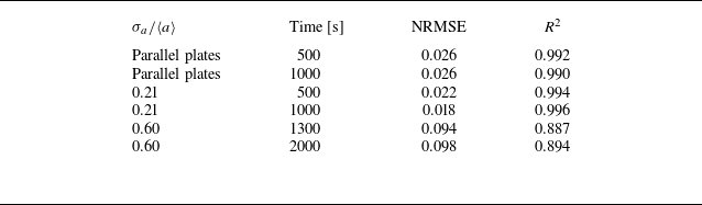


 Open access

