Introduction

The extent of glaciers in the mountainous region of all of Asia, including the former USSR (∼128 000 km2 ; Reference Hirabayashi, Doll and KanaeHirabayashi and others, 2010), is the third largest on Earth, after the Arctic-Greenland and Antarctic regions. Half or more of summer streamflow in major rivers in High Asia is from glacier melt (Reference Barnett, Adam and LettenmaierBarnett and others, 2005), which is particularly important for the Indus and Brahmaputra Rivers and less so for the other major rivers of Asia (Reference Immerzeel, Van Beeke and BierkensImmerzeel and others, 2010). Most crucial is the glacier influence on the rivers in the Aral Basin (Reference Kaser, Grosshauser and MarzeionKaser and others, 2010).

A related potential impact of glacier mass change is on the oceans. Contribution to recent sea-level rise by glaciers in this region, however, has been slight because their rate of thinning is relatively small compared with glaciers elsewhere (Reference Jacob, Wahr, Pfeffer and SwensonJacob and others, 2012). Moreover, some glaciers in the region, particularly in the Karakoram, have not lost mass over recent decades and some have even gained mass (Reference HewittHewitt, 2005; Reference BolchBolch and others, 2012; Reference Gardelle, Berthier and ArnaudGardelle and others, 2012). Mass balance of glaciers in most of High Asia, however, has been becoming more negative (Reference Zemp, Roer, Kaab, Hoelzle, Paul and HaeberliWGMS, 2008a).

Apart from effects of long-term changes in their mass, glaciers exert a significant influence on the seasonal variation of streamflow. They store water in years of high snowfall and release it in years of low snowfall, thus moderating interannual variation of streamflow. They also provide streamflow later in the summer, after seasonal snow has melted, which is the period of high demand for agriculture, hydropower and domestic consumption (Reference Barnett, Adam and LettenmaierBarnett and others, 2005). Delay of flow is caused by temporary englacial storage of spring meltwater and by peak meltwater production occurring in midsummer (Reference Fountain and TangbornFountain and Tang-born, 1985). There is insufficient reservoir capacity in the western part of high-mountain Asia to accommodate the shift in the seasonal cycle by storing early-season melt until it is needed (Reference Barnett, Adam and LettenmaierBarnett and others, 2005). In the eastern part, under the influence of the South Asia monsoon, by contrast, snowfall and subsequent snowmelt occur during the period of need.

The shortage of published measurements of surface mass balance in the region (Reference Cogley PeterboroughCogley, 2011; Reference BolchBolch and others, 2012) hampers calibration of mass-balance models for glaciers there. Of the few mass-balance programs that existed, many have been discontinued since the collapse of the USSR (Reference Zemp, Roer, Kaab, Hoelzle, Paul and HaeberliWGMS, 2008a). Most remaining monitoring programs are glacier inventories obtained by remote sensing. As well as giving glacier extent, they also provide multi-year change in glacier thickness (Reference Berthier, Arnaud, Kumar, Ahmad, Wagnon and ChevallierBerthier and others, 2007; Reference Bolch, Pieczonka and BennBolch and others, 2011), which is closely related to cumulative mass balance over the period between surveys.

Although there is a relative abundance of measurements of change of glacier area and length in the region, such changes are not related to meteorological conditions in a simple way. Change of glacier area is a complicated, nonlinear function of mass balance over a large number of preceding years (Reference Kargel, Cogley, Leonard, Haritashya and ByersKargel and others, 2011). Annual mass balance, by contrast, is a direct, immediate effect of the year’s meteorological conditions. Meteorological variables known to provide a good basis for models of mass balance, especially of summer surface balance (e.g. Reference Rasmussen and ConwayRasmussen and Conway, 2003), are available from 1 January 1948 in the NCEP/NCAR reanalysis database (US National Centers for Environmental Prediction and US National Center for Atmospheric Research; Reference KalnayKalnay and others, 1996; Reference KistlerKistler and others, 2001). It is useful, therefore, to consider spatial and temporal variation of those variables in the region since then.

Methods

Precipitation from the reanalysis database is averaged over 1948-2010 for both winter and summer, and each of these is contoured over 25-508 N, 60-1008 E. Insight into the spatial variation of its seasonality is provided by the mean 19482010 monthly wind vector at 600 hPa (∼4300ma.s.l.), which is an indication of advection of moisture from marine sources, at four selected locations. Temporal variation of annual precipitation at each location is analyzed by fitting a piecewise-constant function; stages of the function are chosen empirically, so that the probability that the values in two successive stages are from the same population is small according to Student’s t-test.

The same piecewise-constant analysis is applied to temperature at each location in the form of the number of annual positive degree-days, PDD, at altitudes representative of the nearby glaciers. Covariance of mean 19482010 monthly temperature and precipitation at each location is demonstrated by plotting them jointly rather than as two separate monthly series.

The PDD is widely used to estimate summer surface balance (Reference BraithwaiteBraithwaite, 1981; Reference OhmuraOhmura, 2001; Reference HockHock, 2003). A simple model

(1)

interpolates linearly in the upper-air temperature profile T(z) at the NCEP/NCARgridpoint nearest the glacier. Here T+(z’) is the PDD and z’ is the middle of the glacier’s altitude range. Coefficients of the linear regression, a and /3, are determined separately for each glacierto minimize the root-mean-square (rms) difference between B* and observed balance, B s, calculated over the glacier’s period of record. In the absence of published observation dates for each year, the summation of T+(z’) is conducted over the entire calendar year, relying on the fact that most temperatures outside the ablation season are negative and thus have little effect on the sum.

For glaciers for which annual records do not exist, published geodetic determinations of mean multi-year annual surface balance, B a, are compared qualitatively with PDD sums and with precipitation, both averaged over the same multi-year period.

Data Sources

The NCEP/NCAR reanalysis database is available globally from Columbia University, with daily records since 1 January 1948, at http://iridl.ldeo.columbia.edu/SOURCES/.NOAA/.NCEP-NCAR/.CDAS-1/.DAILY Temperature and wind are given at many levels in the atmosphere at integer multiples of 2.58 in both latitude and longitude spanning the entire globe. Precipitation is given at a similar array of points.

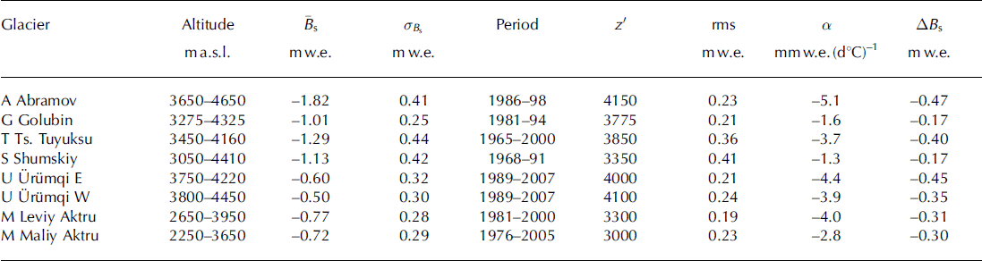
The World Glacier Monitoring Service (Reference Haeberli, Zemp, Kaab, Paul and HoelzleWGMS, 2008b) publishes annual measurements of seasonal surface mass balance, including summer balance for eight glaciers in the region (Table 1 ; Fig. 1).

Table 1.

Positive degree-day (PDD) model results. Recorded statistics of glacier-wide summer surface balance, Bs, its mean, , and standard deviation, a B s, with the rms model error of (Eqn (1)). Observed balance, Bs, from Reference Haeberli, Zemp, Kaab, Paul and HoelzleWGMS (2008b) and previous issues of Fluctuations of glaciers. The PDD factor is a, and sensitivity to +1 8C temperature change is ABs. Letters indicate glacier locations (Figs 1 and 2). Glaciers A and G are in Kyrgyzstan, Tand S in Kazakhstan, U in China and M in Russia

Fig. 1.

Mean 1948–2010 October–April precipitation (cm). A, G, M, S, T, U show locations of glaciers in the Tien Shan (Table 1); R, Y, X, K show glaciers in the eastern Himalaya (Table 3); I the Upper Indus basin in the western Himalaya, and P Pindari Glacier.

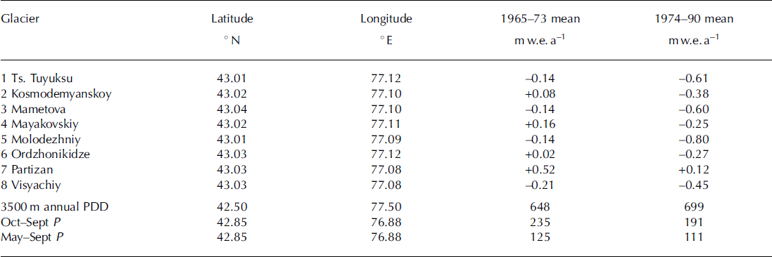
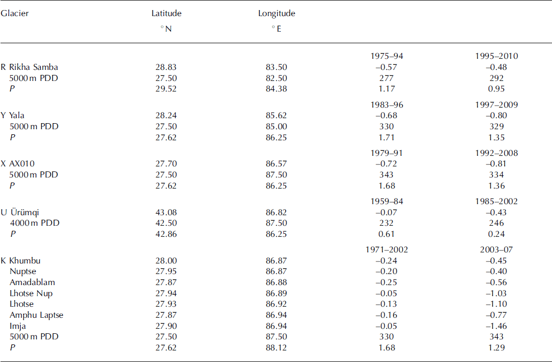
Reference CogleyCogley (2008) gives mean annual surface mass balance, Ba (Table 2), for eight glaciers near each other in the Tien Shan for two multi-year periods. Reference Fujita and NuimuraFujita and Nuimura (2011) present geodetic determinations from several sources for Rikha Samba, Yala and AX010 glaciers, as do Reference Han, Ding, Ye, Liu and JiaoHan and others (2006) for U= rumqi glacier No. 1 (Table 3). For seven other glaciers, near Qomolongma (Mount Everest) (Table 3), Reference Bolch, Pieczonka and BennBolch and others (2011) obtained multi-year (geodetic) mass balances from repeat satellite imagery.

Table 2.

1973 shift in glacier-wide mean surface annual mass balance, Ba. The probability that the Ba values (Reference CogleyCogley, 2008) in the two periods are from the same population is p<0.02 for glaciers 6 and 8, p<0.01 for the others. Location (Tien Shan) is indicated by T in Figures 1 and 2. The values in the bottom three rows are PDD and the nearby precipitation, P (m)

Table 3.

Geodetic glacier-wide surface balance, Ba (m w.e. a–1). Balance values, Ba, for R, Y, X from Reference Fujita and NuimuraFujita and Nuimura (2011), for U from Reference Han, Ding, Ye, Liu and JiaoHan and others (2006), for the others from Reference Bolch, Pieczonka and BennBolch and others (2011). P is May–September precipitation (m w.e.) All are in the eastern Himalaya except for U= rumqi, which is in the Tien Shan

Results

Analysis here is confined to describing the temporal/spatial variation of data from the NCEP/NCAR reanalysis, particularly precipitation and upper-air temperature. Although there are several weather stations in the region, it is not a trivial task to construct a spatially comprehensive description of meteorological conditions from them that is relevant to glacier mass balance. Nevertheless, excellent analyses of meteorological conditions in particular subregions have been published. Among these are Reference Aizen, Aizen, Melack and DozierAizen and others (1997) and Reference BolchBolch (2007) for the Tien Shan, Reference Frauenfeld, Zhang and SerrezeFrauenfeld and others (2005) for the Tibetan Plateau, Reference BolchBolch and others (2012) for the Himalaya, and Reference Shrestha, Wake, Dibb and MayewskiShrestha and others (2000) for Nepal.

Utility of the upper-air temperature and the PDD model (Eqn (1)) is demonstrated for eight glaciers in the region. When driven with these data, the model gives errors (Table 1) that are of the order of observational accuracy. Reference Kayastha, Ageta, Nakawo, Fujita, Sakai and MatsudaKayastha and others (2003) found much larger a values for three glaciers in Nepal.

Variation of precipitation

Spatial variation over central Asia (25-508 N, 60-1008 E) of the mean 1948-2010 winter (October-April) and summer (May-September) precipitation shows a winter maximum in the western part of the region and a summer maximum in the southeastern part (Figs 1 and 2).

Fig. 2.

Mean 1948–2010 May–September precipitation (cm). A, G, M, S, T, U show locations of glaciers in the Tien Shan (Table 1); R, Y, X, K show glaciers in the eastern Himalaya (Table 3); I the Upper Indus basin in the western Himalaya; and P Pindari Glacier.

Annual precipitation has declined over that period at both ends of the Himalaya, but not in the Tien Shan. The coarse grid on which the NCAR/NCEP precipitation is supplied does not resolve smaller-scale features.

Temporal variation of precipitation over 1948-2010 is shown in Figure 3 at three points along the length of the Himalaya and one in the Tien Shan. Consistent with variation at the easternmost point are ice-core measurements from Rongbuk Glacier on Qomolongma by Reference Ren, Jing, Pu and QinRen and others (2006). They showed that annual accumulation decreased rapidly from the 1950s to the 1960s, remained constant until the 1980s, then decreased again.

Fig. 3.

1948–2010 variation of annual precipitation, P (mm), at locations (a) T, (b) I, (c) P and (d) K, shown in Figures 1 and 2. Each series is fit with a piecewise-constant function, stages of which are determined empirically so the probability, p, that the values in two successive stages are from the same population is small according to Student’s t-test. For all pairs of successive stages, p < 0:01, except that p = 0:03 for the 1994–95 shift in (c).

Glacier accumulation depends on the availability of moisture, which is advected by upper-air winds. Wind at 600 hPa (∼4300m a.s.l.) in the Tien Shan is strongly zonal throughout the entire year (Fig. 4a). Seasonal variation of wind direction is qualitatively similar between the middle of the Himalaya (Fig. 4c) and the eastern end (Fig. 4d), with a large variation of direction in summer. In the west (Fig. 4b), the mean wind is weakly westerly during October-April; in summer it veers to the northwest and weakens. In the east it is also westerly during October-April but is much stronger than in the west; in summer, during the monsoon, it becomes roughly southerly but weaker. In the middle of the Himalaya, the westerly wind in winter is weaker than in the east, and during the summer becomes southwesterly.

Fig. 4.

Mean seasonal variation, 1948-2010, of 600 hPa (∼4300m a.s.l.) wind, , at locations (a) T, (b) I, (c) P and (d) K shown in Figures 1 and 2. Direction (heavy curve) and speed (light curve) are shown at monthly resolution.

Correlation of winter surface balance, B w , with winter precipitation at the nearest NCEP/NCAR gridpoint on an annual basis was moderate for Abramov Glacier (r = 0:64 over 13 years) and Golubin Glacier (r = 0:48 over 14 years), but was negligible at four other glaciers in the region. According to Reference Rupper and RoeRupper and Roe (2008), the ‘magnitude of total precipitation and interannual … variability in the Reanalysis output could be off by a factor of 2 or more’. Over multi-year periods, however, the correlation with geodetic balance over the same periods appears to be stronger (Tables 2 and 3).

Variation of temperature

In contrast to the east-west variation in precipitation trends, temperature at the mean altitude of the glaciers, expressed as the annual PDD, shows opposite trends at the two ends. It decreased between 1948-66 and 1967-2010 by ∼ 1 5% in the west and increased by the same amount in the east. The 1948-2010 variation of annual PDD is shown in Figure 5 for the same four locations in the region as in Figures 3 and 4. The striking feature is that the cooling after the mid-1960s in the west occurred at the same time as warming in the east. Reference Fowler and ArcherFowler and Archer (2006) found 1°C cooling in the west after 1961.

Fig. 5.

1948–2010 variation of annual PDD at indicated altitude at locations (a) T, (b) I, (c) P and (d) K shown in Figures 1 and 2. Piecewise-constant function determined as in Figure 3, except that p < 0:01 for all pairs of successive stages.

East-west variation in the Himalaya of the covariance between mean 1948-2010 mean monthly temperature near the middle of the altitude range of the glaciers and mean monthly precipitation (Fig. 6b-d) parallels east-west variation of the wind (Fig. 4), in that the monsoon regime dominates most of the Himalaya. Instead of the summer maximum of precipitation existing in that regime, the west has a winter maximum (Fig. 6b). In the Tien Shan (Fig. 6a) there is a spring maximum of precipitation.

Fig. 6.

Seasonal covariance of monthly precipitation, P (mmdH), and temperature, T(°C), at indicated altitude at locations (a) T, (b) I, (c) Pand (d) K shown in Figures 1 and 2, all averaged over 19482010. Numbers on the curves indicate the months.

Both the 4000 m annual PDD and the summer precipitation changed in 1984 at Urumqi glacier No. 1, contributing to making annual surface balance, B a , more negative (Table 3). Reference Han, Ding, Ye, Liu and JiaoHan and others (2006) found that Ba at Urumqi glacier No. 1 declined from - 0 . 0 7 m a - 1 over 1959-84 to —0:43 m a - 1 over 1985-2002 to —0:74 m a - 1 over 1997-2002. Differencing the last two values yields Ba over 1985-96 of —0:28 m a - 1 , indicating increasingly negative values over the three subperiods during 1959-2002.

Discussion

Spatial and temporal variations of precipitation have received much attention in the literature, which gives valuable insight into the large-scale synoptic conditions underlying the variations shown here (Figs 1-3). In concentrating on some smaller subregions, the literature also furnishes greater detail, for temperature as well as precipitation, than the coarse NCEP/NCAR data.

Storms in the western part of the region (Reference Thayyen and GerganThayyen and Gergan, 2010) are centered at ∼500hPa (∼5500ma.s.l.), southerly monsoons at ∼850hPa (∼1500ma.s.l.). In the Karakoram Himalaya (∼77° E), there are an average of 40 to 50 extratropical storms from the west each year, persisting 2-4 days (Reference BhutiyaniBhutiyani, 1999). Precipitation at Urumqi glacier No. 1 has a summer maximum (Reference Jing, Jiao, Yao, Wang and LiJing and others, 2006). Reference Shrestha, Wake, Dibb and MayewskiShrestha and others (2000) show large interannual and decadal variation in Nepal precipitation and found moderately positive correlation between it and the Southern Oscillation Index (SOI) but none with either the quasi-biennial oscillation (QBO) or the sunspot cycle.

Reference PutkonenPutkonen (2004) found that near Annapurna, in central Nepal, during 1999-2001 the maximum precipitation occurred at ∼3000m. Reference Bookhagen and BurbankBookhagen and Burbank (2010) found that along a south-north transect in the central Himalaya there is a double maximum, a smaller one south of the larger one, but there is a single maximum in the west and in the east. The start of the monsoon varies from year to year, but is always within about 10 days of 1 June (Reference Pai and RajeevanPai and Rajeevan, 2007).

That correlation is often poor between upper-air meteorological conditions and weather station observations does not detract from the utility of the upper-air data in modelling glacier mass balance. The link between upper-air conditions and glacier mass balance might be stronger than between either one of them and conditions at surface weather stations. In the case of U= rumqi glacier No. 1 over 1959– 90, for instance, Reference CaoCao (1998) found that the strong downward shift of mass balance in 1977 was not accompanied by abrupt changes in the record of either summer temperature or annual precipitation at nearby Daxigou weather station.

Improved correlation of upper-air conditions with mass balance might be a consequence of the glaciers being at high altitude, sensing free-air conditions in the atmosphere. In contrast, weather stations are usually at low altitude in confined valleys, where they are more susceptible to surface effects, such as low clouds and aerosols. Another advantage of using the free-air temperatures is it avoids the need to make assumptions about vertical lapse rates that is required when using data from weather stations.

Whereas reanalysis temperatures are valuable estimators of annual variation in summer balance, reanalysis precipitation values are poor estimators of annual variation in winter balance. Poor correlation of NCEP/NCAR reanalysis precipitation and glacier winter balance on an annual basis might be a reflection of the lower reliability of the reanalysis, as noted by Reference Rupper and RoeRupper and Roe (2008). Inaccuracy of annual precipitation values might cancel somewhat when summed over multi-year periods, as suggested by its correlation with multi-year mass balance (Tables 2 and 3).

Conclusions

Although the NCEP/NCAR reanalysis lacks fine spatial resolution, it does provide a uniform, homogeneous record of upper-air temperature that has been successfully used to model interannual variation of glacier-wide summer surface balance, B s, of many glaciers in several other regions. It correlates well at the few glaciers in High Asia where measurements of B s have been published (Table 1). Of particular note is that cooling in the Tien Shan and western Himalaya after the mid-1960s was accompanied by warming in the rest of the Himalaya (Fig. 5).

In contrast to the utility of the reanalysis temperature in estimating B s, precipitation in that database is not a good estimator of interannual variation of winter surface balance. Over multi-year periods, however, it does correlate well with geodetic measurements of mass balance. Spatial distribution of its 1948-2010 averages (Figs 1 and 2) is, therefore, likely to be more realistic, and similarly the seasonal distribution of those averages (Fig. 6).

According to published geodetic determinations, mean glacier-wide annual surface mass balance, Ba, at seven glaciers near Qomolongma (Table 3) declined from an average of — 0:18mw.e. in 1971-2002 to — 0:82mw.e. in 2003-07. Between those two periods, there was only a ∼ 5% increase in the number of 5000 m PDDs, but there was a ∼20% decrease in precipitation. This was also the case at three other glaciers in Nepal, but warming played a stronger role elsewhere. At eight nearby glaciers in the Tien Shan (Table 2) there was a pronounced decline in surface mass balance between 1965-73 and 1974-90 that was accompanied by ∼20% decrease in precipitation and ∼10% increase in 3500m PDD, near the middle of the altitude range of the glaciers.

The small and declining number of traditional mass-balance programs makes calibrating mass-balance models difficult. Because the effects of meteorological variables on mass-balance processes are known in principle, however, it is worth considering spatial and temporal variations of those variables. They are described here over 25–508 N, 60–1008 E for 1948–2010. In the likely absence of rejuvenated programs, future variations of the variables, along with known approximate relations between them and surface mass balance, can create a rough proxy for variation of mass balance.