2.1 Unsteady velocity fields

The unsteady loading on the downstream propeller blades at a given radial location is calculated using an equivalent two-dimensional problem where the wakes from an upstream cascade of blades interact with the blades of a downstream cascade. This situation is illustrated in figure 2. The formulation presented here will make use of a Cartesian coordinate system $\{x_{1},y_{1}\}$ , where $x_{1}$ is an axial coordinate defined such that the airflow has Mach number $M_{x}$ in the positive $x_{1}$ -direction and $y_{1}$ is a tangential coordinate which is parallel to the direction in which the blade rows translate. Note that, as the models for wake convection and rear rotor unsteady response follow the usual conventions, the $x_{i}$ -axes are directed downstream, unlike the cylindrical polar system shown in figure 1 in which the $x$ -axis is directed upstream. The upstream and downstream blades translate in the negative and positive $y$ -directions at Mach numbers $\unicode[STIX]{x1D6FA}_{1}r/c_{0}$ and $\unicode[STIX]{x1D6FA}_{2}r/c_{0}$ respectively. At time $\unicode[STIX]{x1D70F}=0$ the pitch-change axis of the front propeller reference blade is aligned with the pitch-change axis of the rear propeller reference blade at $y_{1}/D=0$ and the spacing between the mid-chord positions of the blades on each cascade in the $y_{1}$ -direction is equal to $2\unicode[STIX]{x03C0}r/B$ . The blades are modelled as infinitely thin flat plates which are aligned with the local flow direction but otherwise have identical characteristics (chord length, sweep, lean and drag coefficient) to the actual propeller blade at that particular radius. Also, the effect of the flow induced by the propellers is neglected such that the stagger angle, $\unicode[STIX]{x1D6FC}$ , of each blade is defined by $\tan \unicode[STIX]{x1D6FC}=zM_{T}/M_{x}$ , where $z=2r/D$ and $M_{T}=\unicode[STIX]{x1D6FA}D/2c_{0}$ . The Mach number of the flow relative to each blade is denoted $M_{r}$ . These assumptions are entirely consistent with Hanson’s helicoidal surface theory (Reference Hanson1983, Reference Hanson1985) for both single- and contra-rotating propellers which forms the basis for the acoustic radiation calculations in § 2.3.

In order to describe the development of the wakes from the upstream cascade it is convenient to introduce two coordinate systems which are locked to the upstream blade row and have origins located at the mid-chord of the upstream reference blade. The $\{x_{1},y_{1}\}$ coordinate system has coordinates which are parallel to the global $\{x,y\}$ coordinate system. The $\{X_{1},Y_{1}\}$ coordinate system has coordinates parallel to the chordwise and chord-normal directions and is related to the $\{x_{1},y_{1}\}$ coordinate system by

(2.1) $$\begin{eqnarray}\displaystyle & X_{1}=x_{1}\cos \unicode[STIX]{x1D6FC}_{1}+y_{1}\sin \unicode[STIX]{x1D6FC}_{1}, & \displaystyle\end{eqnarray}$$

(2.2) $$\begin{eqnarray}\displaystyle & Y_{1}=-x_{1}\sin \unicode[STIX]{x1D6FC}_{1}+y_{1}\cos \unicode[STIX]{x1D6FC}_{1}. & \displaystyle\end{eqnarray}$$

The velocity deficit from the upstream reference blade is taken to be completely general and is denoted as the vector $\overline{\boldsymbol{u}}^{\prime }(x_{1},y_{1})$ . Note that this deficit velocity is most naturally expressed in the $\{X_{1},Y_{1}\}$ coordinate system as, following our assumption that the blade has no thickness and does not turn the flow, the wake centreline remains aligned with the $X_{1}$ coordinate. The upstream propeller blades are assumed to be evenly spaced and identical and thus the mean velocity deficit produced by the upstream cascade, $\overline{\boldsymbol{v}}^{\prime }$ , is given by

(2.3) $$\begin{eqnarray}\overline{\boldsymbol{v}}^{\prime }=\mathop{\sum }_{n_{1}=-\infty }^{\infty }\overline{\boldsymbol{u}}^{\prime }\left(x_{1},y_{1}+\frac{2\unicode[STIX]{x03C0}r}{B_{1}}n_{1}\right).\end{eqnarray}$$

In order to calculate the response of the downstream blade row, the wakes are assumed to be frozen in the vicinity of the leading edge of the downstream blade row. Applying Poisson’s summation theorem to (2.3), the velocity deficit incident on the downstream blade row is given as a sum of Fourier harmonics by

(2.4) $$\begin{eqnarray}\overline{\boldsymbol{v}}^{\prime }=\mathop{\sum }_{n_{1}=-\infty }^{\infty }\boldsymbol{u}_{n_{1}}\exp \left\{\text{i}\frac{n_{1}B_{1}}{r}y_{1}-\text{i}\frac{n_{1}B_{1}}{r}x_{1}\tan \unicode[STIX]{x1D6FC}_{1}\right\},\end{eqnarray}$$

where

(2.5) $$\begin{eqnarray}\boldsymbol{u}_{n_{1}}=\frac{B_{1}}{2\unicode[STIX]{x03C0}r}\int _{-\infty }^{\infty }\overline{\boldsymbol{u}}^{\prime }(x_{1},y_{c}+x_{1}\tan \unicode[STIX]{x1D6FC}_{1})\exp \left\{-\text{i}\frac{n_{1}B_{1}}{r}y_{c}\right\}\text{d}y_{c},\end{eqnarray}$$

and we have used the translated coordinate $y_{c}=y_{1}-x_{1}\tan \unicode[STIX]{x1D6FC}_{1}$ to centre the Fourier integral on the wake centreline.

In order to calculate the unsteady loading on the downstream blade row, it is necessary to express $\overline{\boldsymbol{v}}^{\prime }$ in a coordinate system fixed to the rear propeller blades. For this purpose we introduce a blade locked axial/tangential coordinate system $\{x_{2},y_{2}\}$ which is parallel to the $\{x_{1},y_{1}\}$ coordinates and has an origin located at the leading edge of the reference blade on the downstream blade row. The $\{x_{2},y_{2}\}$ coordinate system is related to the $\{x_{1},y_{1}\}$ coordinate system by

(2.6) $$\begin{eqnarray}\displaystyle & \displaystyle x_{1}=x_{2}+g-s_{1}\cos \unicode[STIX]{x1D6FC}_{1}+\left(s_{2}-\frac{c_{2}}{2}\right)\cos \unicode[STIX]{x1D6FC}_{2}, & \displaystyle\end{eqnarray}$$

(2.7) $$\begin{eqnarray}\displaystyle & \displaystyle y_{1}=y_{2}+(\unicode[STIX]{x1D6FA}_{1}+\unicode[STIX]{x1D6FA}_{2})r\unicode[STIX]{x1D70F}-s_{1}\sin \unicode[STIX]{x1D6FC}_{1}-\left(s_{2}-\frac{c_{2}}{2}\right)\sin \unicode[STIX]{x1D6FC}_{2}. & \displaystyle\end{eqnarray}$$

One final coordinate transformation is required in order to express $\overline{\boldsymbol{v}}^{\prime }$ in terms of the chordwise/chord-normal coordinate system of the downstream reference blade, $\{X_{2},Y_{2}\}$ , which is defined by

(2.8) $$\begin{eqnarray}\displaystyle & x_{2}=X_{2}\cos \unicode[STIX]{x1D6FC}_{2}+Y_{2}\sin \unicode[STIX]{x1D6FC}_{2}, & \displaystyle\end{eqnarray}$$

(2.9) $$\begin{eqnarray}\displaystyle & y_{2}=-X_{2}\sin \unicode[STIX]{x1D6FC}_{2}+Y_{2}\cos \unicode[STIX]{x1D6FC}_{2}. & \displaystyle\end{eqnarray}$$

Using (2.6)–(2.9) in (2.4) enables the (arbitrary) velocity deficit from the $B_{1}$ front row blades to be expressed in the $\{X_{2},Y_{2}\}$ coordinate system as

(2.10) $$\begin{eqnarray}\overline{\boldsymbol{v}}^{\prime }=\mathop{\sum }_{n_{1}=-\infty }^{\infty }\boldsymbol{u}_{n_{1}}\exp \left\{\text{i}n_{1}B_{1}(\unicode[STIX]{x1D6FA}_{1}+\unicode[STIX]{x1D6FA}_{2})\unicode[STIX]{x1D70F}-\text{i}k_{X}X_{2}-\text{i}k_{Y}Y_{2}-\text{i}k_{X}\left(s_{2}-\frac{c_{2}}{2}\right)-\text{i}k_{Y_{1}}g\sin \unicode[STIX]{x1D6FC}_{1}\right\},\end{eqnarray}$$

where the wavenumbers $k_{X}$ , $k_{Y}$ and $k_{Y_{1}}$ are defined as

(2.11) $$\begin{eqnarray}\displaystyle & \displaystyle k_{X}=\frac{n_{1}B_{1}}{r\cos \unicode[STIX]{x1D6FC}_{1}}\sin (\unicode[STIX]{x1D6FC}_{1}+\unicode[STIX]{x1D6FC}_{2})=\frac{2n_{1}B_{1}}{DM_{r_{2}}}[M_{T_{1}}+M_{T_{2}}], & \displaystyle\end{eqnarray}$$

(2.12) $$\begin{eqnarray}\displaystyle & \displaystyle k_{Y}=-\frac{n_{1}B_{1}}{r\cos \unicode[STIX]{x1D6FC}_{1}}\cos (\unicode[STIX]{x1D6FC}_{1}+\unicode[STIX]{x1D6FC}_{2})=-\frac{2n_{1}B_{1}}{DM_{r_{2}}}\left[\frac{M_{x}}{z}-z\frac{M_{T_{1}}M_{T_{2}}}{M_{x}}\right], & \displaystyle\end{eqnarray}$$

and

(2.13) $$\begin{eqnarray}k_{Y_{1}}=\frac{n_{1}B_{1}}{r\cos \unicode[STIX]{x1D6FC}_{1}}=\frac{2n_{1}B_{1}M_{r_{1}}}{zDM_{x}}.\end{eqnarray}$$

The mean upwash velocity (which is the component of velocity normal to the rear row blades, or in the $Y_{2}$ direction) onto the downstream reference blade is given by $w=\boldsymbol{j}_{Y_{2}}\boldsymbol{\cdot }\overline{\boldsymbol{v}}^{\prime }$ , where $\boldsymbol{j}_{Y_{2}}$ is a unit vector aligned with the $Y_{2}$ coordinate. The upwash at the chord line of the reference blade of the downstream blade row (on which $Y_{2}=0$ ) is thus equal to a sum of convected harmonic gusts

(2.14) $$\begin{eqnarray}w=\mathop{\sum }_{n_{1}=-\infty }^{\infty }w_{n_{1}}\exp \{\text{i}k_{X}(U_{r_{2}}\unicode[STIX]{x1D70F}-X_{2})-\text{i}k_{Y}Y_{2}\},\end{eqnarray}$$

where $U_{r_{2}}$ is the velocity magnitude of the air relative to the downstream blade and

(2.15) $$\begin{eqnarray}w_{n_{1}}={\hat{w}}_{n_{1}}\exp \left\{-\text{i}k_{X}\left(s_{2}-\frac{c_{2}}{2}\right)-\text{i}k_{Y_{1}}g\sin \unicode[STIX]{x1D6FC}_{1}\right\},\end{eqnarray}$$

with ${\hat{w}}_{n_{1}}=\boldsymbol{j}_{Y_{2}}\boldsymbol{\cdot }\boldsymbol{u}_{n_{1}}$ .

The total unsteady lift force per unit area acting on the chord line of the reference blade can be expressed as the sum of the unsteady ‘response’ of the blade to all of the upwash harmonics i.e.

(2.16) $$\begin{eqnarray}\unicode[STIX]{x0394}p(\overline{X}_{2})=\mathop{\sum }_{n_{1}=-\infty }^{\infty }\unicode[STIX]{x0394}p_{n_{1}}(\overline{X}_{2})\exp \{\text{i}n_{1}B_{1}(\unicode[STIX]{x1D6FA}_{1}+\unicode[STIX]{x1D6FA}_{2})\unicode[STIX]{x1D70F}\},\end{eqnarray}$$

where $\unicode[STIX]{x0394}p_{n_{1}}(\overline{X}_{2})\exp \{\text{i}n_{1}B_{1}(\unicode[STIX]{x1D6FA}_{1}+\unicode[STIX]{x1D6FA}_{2})\unicode[STIX]{x1D70F}\}$ is the response of the reference blade to a gust of the form $w_{n_{1}}\exp \{\text{i}k_{X}(U_{r_{2}}\unicode[STIX]{x1D70F}-X_{2})-\text{i}k_{Y}Y_{2}\}$ and $\unicode[STIX]{x0394}p_{n_{1}}$ can be expressed in the form

(2.17) $$\begin{eqnarray}\unicode[STIX]{x0394}p_{n_{1}}(\overline{X}_{2})=2\unicode[STIX]{x03C0}\unicode[STIX]{x1D70C}_{0}U_{r_{2}}w_{n_{1}}\mathbb{S}(\unicode[STIX]{x1D70E}_{2},M_{r_{2}},\overline{X}_{2},\unicode[STIX]{x1D6EC}),\end{eqnarray}$$

where $\overline{X}_{2}=2X_{2}/c_{2}$ is a dimensionless chordwise coordinate, $\unicode[STIX]{x1D70E}_{2}=k_{X}c_{2}/2$ is the reduced frequency, $\unicode[STIX]{x1D6EC}$ is a local blade leading-edge sweep angle (defined in the following section) and $\mathbb{S}$ is a non-dimensional response function.

2.2 Unsteady aerodynamic response

In § 2.1, above, we considered the aerodynamics of a purely two-dimensional cascade of blades in terms of the wake flows from the upstream blades. However, for the unsteady response of the downstream blades it is important that we account for the local three-dimensional response that occurs when the rear blades are swept. Our model for the propellers follows the helicoidal blade approach of Hanson (Reference Hanson1983) so that there is no wake swirl and, consequently, our consideration of oblique incidence is restricted solely to blade sweep effects.

We consider an infinitely small blade element of spanwise length $\text{d}z_{2}$ at radial location $z_{2}$ where $z_{2}=2r/D$ is the normalised radius of the rear row. Since, in this paper, the aerodynamics is considered to be quasi-two-dimensional, we must ‘unwrap’ and ‘untwist’ the blades to produce an equivalent interaction problem of a gust with a semi-infinite flat plate in a Cartesian system. We use cylindrical polar coordinates $(z_{2},\unicode[STIX]{x1D719}_{2},x_{2})$ for the blades and $(Z_{2},Y_{2},X_{2})$ for the ‘unwrapped’ system, and both sets of coordinates are locked to the rear row with the $(Z_{2},Y_{2},X_{2})$ coordinate system having its origin at the local blade leading-edge location.

The Cartesian and cylindrical polar systems would normally be linked by the relationships $Z_{2}=h_{z}(z_{2}-z_{l})$ , $Y_{2}=~h_{\unicode[STIX]{x1D719}}\unicode[STIX]{x1D719}_{2}$ , $X_{2}=h_{x}x_{2}$ where $z_{l}$ is the local dimensionless radius and $h_{z}=1$ , $h_{\unicode[STIX]{x1D719}}=z_{2}$ , $h_{x}=1$ are the Lamé coefficients. However, for a purely Cartesian system, these coefficients must be constant thus we use $h_{\unicode[STIX]{x1D719}}=z_{l}$ where $z_{l}$ is taken to be constant at the value of the local non-dimensional radius. Thus, for an infinitely small element of the blade leading edge lying between $(z_{2},\unicode[STIX]{x1D719}_{LE}(z_{2}),x_{LE}(z_{2}))$ and $(z_{2}+\text{d}z_{2},\unicode[STIX]{x1D719}_{LE}(z_{2}+\text{d}z_{2}),x_{LE}(z_{2}+\text{d}z_{2}))$ , where $\unicode[STIX]{x1D719}_{LE}=\unicode[STIX]{x1D719}_{LE}(z_{2})$ , $x_{LE}=x_{LE}(z_{2})$ represent the azimuthal and axial locations of the blade leading edge (see figure 3), the elemental leading edge is given by

(2.18a-c ) $$\begin{eqnarray}\text{d}Z_{2}=\text{d}z_{2},\quad \text{d}Y_{LE}=z_{l}\,\text{d}\unicode[STIX]{x1D719}_{LE}=z_{l}\frac{\text{d}\unicode[STIX]{x1D719}_{LE}}{\text{d}z_{2}}\,\text{d}z_{2},\quad \text{d}X_{LE}=\text{d}x_{LE}=\frac{\text{d}x_{LE}}{\text{d}z_{2}}\,\text{d}z_{2}.\end{eqnarray}$$

In cylindrical blade-fixed coordinates, the leading edge of the rear blade, which varies as a function of $z_{2}$ , lies (relative to its unswept location) at

(2.19a-c ) $$\begin{eqnarray}z_{2},\quad \unicode[STIX]{x1D719}_{LE}(z_{2})=-\frac{\overline{s}_{L}\sin \unicode[STIX]{x1D6FC}_{2}}{z_{2}}=-M_{t}\frac{\overline{s}_{L}(z_{2})}{M_{r_{2}}(z_{2})},\quad x_{LE}(z_{2})=-\overline{s}_{L}\cos \unicode[STIX]{x1D6FC}_{2}=-M_{x}\frac{\overline{s}_{L}(z_{2})}{M_{r_{2}}(z_{2})},\quad\end{eqnarray}$$

where $\overline{s}_{L}=2(s_{2}-c_{2}/2)/D$ , so that, combining the axial and azimuthal terms, and using (2.18) and (2.19), we find that elemental changes $\text{d}S_{2}$ in the non-dimensional sweep in the new Cartesian system – at a fixed radius $Z_{2}$ – are given by $\text{d}S_{2}^{2}=\text{d}X_{LE}^{2}+\text{d}Y_{LE}^{2}$ or

(2.20) $$\begin{eqnarray}\frac{\text{d}S_{2}}{\text{d}Z_{2}}=\sqrt{\left(\frac{\text{d}X_{LE}}{\text{d}Z_{2}}\right)^{2}+\left(\frac{\text{d}Y_{LE}}{\text{d}Z_{2}}\right)^{2}}=\sqrt{M_{x}^{2}+z_{l}^{2}M_{t}^{2}}\frac{\text{d}}{\text{d}z_{2}}\left(\frac{\overline{s}_{L}}{M_{r_{2}}}\right)=M_{r_{l}}\frac{\text{d}}{\text{d}z_{2}}\left(\frac{\overline{s}_{L}}{M_{r_{2}}}\right).\end{eqnarray}$$

The value $\text{d}S_{2}$ combines the axial and azimuthal movement of the leading-edge location. The value $M_{r_{l}}$ in (2.20) represents the local relative Mach number in the unwrapped system which is taken to be constant. The net sweep angle of the blade in the unwrapped system is defined as $\unicode[STIX]{x1D6EC}$ with

(2.21) $$\begin{eqnarray}\tan \unicode[STIX]{x1D6EC}=\frac{\text{d}S_{2}}{\text{d}Z_{2}}=M_{r_{l}}\frac{\text{d}}{\text{d}z_{2}}\left(\frac{\overline{s}_{L}}{M_{r_{2}}}\right).\end{eqnarray}$$

For reference here we note that an element of leading-edge arc length $\unicode[STIX]{x1D564}$ is given by

(2.22) $$\begin{eqnarray}\text{d}\unicode[STIX]{x1D564}^{2}=\text{d}Z_{2}^{2}+\text{d}S_{2}^{2}=\left\{1+\left[M_{r_{l}}\frac{\text{d}}{\text{d}z_{2}}\left(\frac{\overline{s}_{L}}{M_{r_{2}}}\right)\right]^{2}\right\}\text{d}z_{2}^{2}\end{eqnarray}$$

or, equivalently, by $\text{d}\unicode[STIX]{x1D564}=\text{d}z_{2}/\text{cos}\unicode[STIX]{x1D6EC}$ so that the trace velocity of any disturbance along the leading edge of a rear blade is $\sec \unicode[STIX]{x1D6EC}$ times that of the radial disturbance velocity. The swept distance $S_{2}$ in the Cartesian system can be obtained by integrating (2.21), using $\text{d}Z_{2}=\text{d}z_{2}$ , from (2.18), and the fact that $M_{r_{l}}$ is constant, to get $S_{2}=(M_{r_{l}}/M_{r_{2}})\overline{s}_{L}=\overline{s}_{L}$ at $z_{2}=z_{l}$ .

Figure 3.

Segment of an annulus which lies between $z_{2}$ and $z_{2}+\text{d}z_{2}$ (a). Corresponding unwrapped segment (b).

Using the geometry of the original wrapped system, given in § 2, it is easy to show that a wake centreline, lying along Hanson’s helicoidal surface and passing through the pitch-change axis of the rear blade, travels a non-dimensional distance $\overline{s}_{L}(\cos \unicode[STIX]{x1D6FC}_{2}\tan \unicode[STIX]{x1D6FC}_{1}+\sin \unicode[STIX]{x1D6FC}_{2})=z_{2}(M_{t_{1}}+M_{t_{2}})\overline{s}_{L}/M_{r_{2}}$ in the negative $\unicode[STIX]{x1D719}_{2}$ direction to reach the blade leading edge at a non-dimensional speed $z_{2}(M_{t_{1}}+M_{t_{2}})$ relative to the rear blade row. The radial component of the trace Mach number is thus easily obtained as $[\text{d}/\text{d}z_{2}(\overline{s}_{L}/M_{r_{2}})]^{-1}$ . In the new unwrapped and untwisted system, the blades are represented by a cascade with non-dimensional leading-edge sweep $S_{2}$ and sweep angle $\unicode[STIX]{x1D6EC}$ . The front and rear blade rows translate in opposite $\unicode[STIX]{x1D719}_{2}$ directions at Mach numbers $z_{l}M_{t_{1}}$ and $z_{l}M_{t_{2}}$ , respectively, and the relative Mach number of the flow parallel to the rear blade is $M_{r_{l}}$ . A similar geometric analysis shows that the wake centreline travels a non-dimensional distance $z_{l}(M_{t_{1}}+M_{t_{2}})S_{2}/M_{r_{l}}$ at a non-dimensional speed $z_{l}(M_{t_{1}}+M_{t_{2}})$ so that the radial component of the trace Mach number along the leading edge of the cascade is obtained as $M_{r_{l}}/(\text{d}S_{2}/\text{d}Z_{2})=M_{r_{l}}/\tan \unicode[STIX]{x1D6EC}$ which, from (2.21), is identical to that along the leading edge of the downstream blade row in the original wrapped system.

Figure 4.

Definition of blade leading-edge sweep and local coordinate systems.

In order to consider the response of the swept blade in the new unwrapped system, we define new coordinates $(\unicode[STIX]{x1D709},\unicode[STIX]{x1D712},\unicode[STIX]{x1D701})$ aligned to the local swept blade with

(2.23a-c ) $$\begin{eqnarray}X_{2}=\unicode[STIX]{x1D709}\cos \unicode[STIX]{x1D6EC}+\unicode[STIX]{x1D701}\sin \unicode[STIX]{x1D6EC},\quad Y_{2}=\unicode[STIX]{x1D712},\quad Z_{2}=-\unicode[STIX]{x1D709}\sin \unicode[STIX]{x1D6EC}+\unicode[STIX]{x1D701}\cos \unicode[STIX]{x1D6EC},\end{eqnarray}$$

where $Z_{2}$ is a normalised radius with its origin centred on the local radial station at which the gust interaction is taking place and $X_{2}$ is the chordwise or streamwise direction. In this coordinate system, shown in figure 4, each incident harmonic gust defined by (2.14) can then be rewritten as

(2.24) $$\begin{eqnarray}w=w_{n_{1}}\exp \{\text{i}(k_{\unicode[STIX]{x1D709}}U_{\unicode[STIX]{x1D709}}+k_{\unicode[STIX]{x1D701}}U_{\unicode[STIX]{x1D701}})\unicode[STIX]{x1D70F}-\text{i}k_{\unicode[STIX]{x1D709}}\unicode[STIX]{x1D709}-\text{i}k_{\unicode[STIX]{x1D701}}\unicode[STIX]{x1D701}-\text{i}k_{\unicode[STIX]{x1D712}}\unicode[STIX]{x1D712}\},\end{eqnarray}$$

where

(2.25a-e ) $$\begin{eqnarray}k_{\unicode[STIX]{x1D709}}=k_{X}\cos \unicode[STIX]{x1D6EC},\quad k_{\unicode[STIX]{x1D701}}=k_{X}\sin \unicode[STIX]{x1D6EC},\quad k_{\unicode[STIX]{x1D712}}=k_{Y},\quad U_{\unicode[STIX]{x1D709}}=U_{r_{2}}\cos \unicode[STIX]{x1D6EC},\quad U_{\unicode[STIX]{x1D701}}=U_{r_{2}}\sin \unicode[STIX]{x1D6EC}.\end{eqnarray}$$

If we assume that, at a local radial station $z$ , the swept blade can be considered to be equivalent to a section of an infinite swept aerofoil (as shown in figure 4) with velocities $U_{\unicode[STIX]{x1D709}}$ and $U_{\unicode[STIX]{x1D701}}$ in the $\unicode[STIX]{x1D709}$ and $\unicode[STIX]{x1D701}$ directions and $(\unicode[STIX]{x1D709},\unicode[STIX]{x1D712},\unicode[STIX]{x1D701})$ wavenumbers $(k_{\unicode[STIX]{x1D709}},k_{\unicode[STIX]{x1D712}},k_{\unicode[STIX]{x1D701}})$ , then the high-frequency solution to the linearised gust interaction problem in subsonic compressible flow can be obtained from a Wiener–Hopf analysis, or taken directly from Adamczyk (Reference Adamczyk1974). (The Wiener–Hopf analysis assumes that the aerofoil is semi-infinite in the chordwise direction and represents the interaction of the gust with the leading edge. As we are only interested in predicting the leading-order behaviour of the acoustic field, we apply no correction for the effect of the aerofoil’s trailing edge. A discussion of the range of validity of this expression applied to swept thin aerofoils of finite chord length is contained in Adamczyk (Reference Adamczyk1974). For unswept blades Goldstein (Reference Goldstein1976) states that the total unsteady lift force per unit length calculated using this expression is accurate to within 10% when $M_{r_{2}}\unicode[STIX]{x1D70E}_{2}/(1-M_{r_{2}}^{2})>1$ . That expression can be taken to be satisfied here as $\unicode[STIX]{x1D70E}_{2}$ is directly proportional to $B_{1}$ and, in line with our high blade number assumption, $B_{1}\gg 1$ .) Our notation is somewhat different to Adamczyk’s, but a little manipulation produces

(2.26) $$\begin{eqnarray}\mathbb{S}=\frac{\text{e}^{-\text{i}\unicode[STIX]{x03C0}/4-\text{i}\unicode[STIX]{x1D70E}_{\unicode[STIX]{x1D701}}\overline{\unicode[STIX]{x1D701}}}}{\unicode[STIX]{x03C0}\sqrt{\unicode[STIX]{x03C0}\overline{\unicode[STIX]{x1D709}}}}\frac{\exp \left[{\displaystyle \frac{\text{i}\unicode[STIX]{x1D70E}_{\unicode[STIX]{x1D709}}M_{\unicode[STIX]{x1D709}}^{2}-\text{i}\sqrt{M_{\unicode[STIX]{x1D709}}^{2}\unicode[STIX]{x1D70E}_{\unicode[STIX]{x1D709}}^{2}-(1-M_{\unicode[STIX]{x1D709}}^{2})\unicode[STIX]{x1D70E}_{\unicode[STIX]{x1D701}}^{2}}}{(1-M_{\unicode[STIX]{x1D709}}^{2})}}\overline{\unicode[STIX]{x1D709}}\right]}{\sqrt{\unicode[STIX]{x1D70E}_{\unicode[STIX]{x1D709}}+\sqrt{M_{\unicode[STIX]{x1D709}}^{2}\unicode[STIX]{x1D70E}_{\unicode[STIX]{x1D709}}^{2}-(1-M_{\unicode[STIX]{x1D709}}^{2})\unicode[STIX]{x1D70E}_{\unicode[STIX]{x1D701}}^{2}}}},\end{eqnarray}$$

where we have defined the reduced frequencies $\unicode[STIX]{x1D70E}_{\unicode[STIX]{x1D709}}=k_{\unicode[STIX]{x1D709}}c_{\unicode[STIX]{x1D709}}/2$ , $\unicode[STIX]{x1D70E}_{\unicode[STIX]{x1D701}}=k_{\unicode[STIX]{x1D701}}c_{\unicode[STIX]{x1D709}}/2$ , $\overline{\unicode[STIX]{x1D709}}$ and $\overline{\unicode[STIX]{x1D701}}$ are coordinates normalised by $c_{\unicode[STIX]{x1D709}}/2$ , the normal chord distance is given by $c_{\unicode[STIX]{x1D709}}=c_{2}\cos \unicode[STIX]{x1D6EC}$ and our new chordwise coordinate $\overline{\unicode[STIX]{x1D709}}$ has its origin at the leading edge. The dimensional unsteady response is given by $\unicode[STIX]{x0394}p_{n_{1}}(\overline{\unicode[STIX]{x1D709}})=2\unicode[STIX]{x03C0}\unicode[STIX]{x1D70C}_{0}U_{r_{2}}w_{n_{1}}\mathbb{S}$ which is consistent with (2.17) but with the dimensional velocity 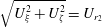$\sqrt{U_{\unicode[STIX]{x1D709}}^{2}+U_{\unicode[STIX]{x1D701}}^{2}}=U_{r_{2}}$ .

After some manipulation, we obtain the unsteady response of the blade to an oblique gust as

(2.27) $$\begin{eqnarray}\mathbb{S}(\unicode[STIX]{x1D70E}_{2},M_{r_{2}},\unicode[STIX]{x1D6EC},X_{2})=\frac{\text{e}^{-\text{i}\unicode[STIX]{x03C0}/4}\exp \left\{\text{i}\unicode[STIX]{x1D70E}_{2}{\displaystyle \frac{\left[(M_{r_{2}}^{2}-\tan ^{2}\unicode[STIX]{x1D6EC})-\sqrt{M_{r_{2}}^{2}-\tan ^{2}\unicode[STIX]{x1D6EC}}\right]}{[1-(M_{r_{2}}^{2}-\tan ^{2}\unicode[STIX]{x1D6EC})]}}\overline{X}_{2}\right\}}{\unicode[STIX]{x03C0}\sqrt{\unicode[STIX]{x03C0}\unicode[STIX]{x1D70E}_{2}\overline{X}_{2}}\sqrt{1+\sqrt{M_{r_{2}}^{2}-\tan ^{2}\unicode[STIX]{x1D6EC}}}},\end{eqnarray}$$

where $\unicode[STIX]{x1D70E}_{2}=k_{X}c_{2}/2$ and we have switched back to the $(X_{2},Y_{2},Z_{2})$ coordinate system and omitted the terms in $Z_{2}$ , since – for an oblique interaction calculation with a propeller blade at a fixed radius – we must have $Z_{2}=0$ . In (2.27) we see that the unsteady response switches from a pure phase variation along the chord to one which is exponentially decaying when $\tan \unicode[STIX]{x1D6EC}>M_{r_{2}}$ . It is interesting to note here, from the definition of the sweep angle in (2.21), that the change occurs at the radius at which $\tan \unicode[STIX]{x1D6EC}=\tan \unicode[STIX]{x1D6EC}^{\ast }=M_{r_{2}}$ , in agreement with the solutions of Adamczyk (Reference Adamczyk1974) and Envia & Kerschen (Reference Envia and Kerschen1990) who, along with Graham (Reference Graham1970), discussed the transition point between these super-critical and sub-critical interactions in some detail. (Our solution is simplified relative to Envia & Kerschen’s as we have no wake lean, because of the absence of swirl in our case, and no spanwise wake phase angle due to our assumption of quasi-two-dimensional wakes.) Roger et al. (Reference Roger, Schram and Moreau2014) and Quaglia et al. (Reference Quaglia, Léonard, Moreau and Roger2017) presented similar methods for calculating the response of a swept blade to a harmonic gust. It is useful to observe that, in our case, $\tan \unicode[STIX]{x1D6EC}^{\ast }=M_{r_{2}}$ when

(2.28) $$\begin{eqnarray}\frac{\text{d}}{\text{d}z}\left(\frac{\overline{s}_{L}}{M_{r_{2}}}\right)=1.\end{eqnarray}$$

By choosing the appropriate branch cut, the solution for $\unicode[STIX]{x1D6EC}>\unicode[STIX]{x1D6EC}^{\ast }$ is

(2.29) $$\begin{eqnarray}\displaystyle \mathbb{S}(\unicode[STIX]{x1D70E}_{2},M_{r_{2}},\unicode[STIX]{x1D6EC},X_{2}) & = & \displaystyle \text{e}^{-\text{i}(\unicode[STIX]{x03C0}/4)+(\text{i}/2)\tan ^{-1}\sqrt{\tan ^{2}\unicode[STIX]{x1D6EC}-M_{r_{2}}^{2}}}\nonumber\\ \displaystyle & & \displaystyle \times \,\frac{\exp \left\{\unicode[STIX]{x1D70E}_{2}{\displaystyle \frac{\left[-\text{i}(\tan ^{2}\unicode[STIX]{x1D6EC}-M_{r_{2}}^{2})-\sqrt{\tan ^{2}\unicode[STIX]{x1D6EC}-M_{r_{2}}^{2}}\right]}{[1+(\tan ^{2}\unicode[STIX]{x1D6EC}-M_{r_{2}}^{2})]}}\overline{X}_{2}\right\}}{\unicode[STIX]{x03C0}\sqrt{\unicode[STIX]{x03C0}\unicode[STIX]{x1D70E}_{2}\overline{X}_{2}}[1+(\tan ^{2}\unicode[STIX]{x1D6EC}-M_{r_{2}}^{2})]^{1/4}},\qquad\end{eqnarray}$$

where we have incorporated all the phase terms into the exponential argument.

2.3 Acoustic radiation

Following the derivation presented by Hanson (Reference Hanson1985), the far-field tonal sound pressure at ‘emission radius’ $R_{e}$ , ‘emission polar angle’ $\unicode[STIX]{x1D703}_{e}$ (defined such that $\unicode[STIX]{x1D703}_{e}=0$ is upstream of the rotor), azimuthal angle $\unicode[STIX]{x1D719}$ and time $t$ (where source time $\unicode[STIX]{x1D70F}=t-R_{e}/c_{0}$ for a source located at the origin of the coordinate system) produced by the periodic lift forces on the downstream propeller of a contra-rotating open rotor due to the unsteady velocity fields from the upstream propeller can be shown to be given by the following expression

(2.30) $$\begin{eqnarray}p=\frac{\text{i}\unicode[STIX]{x1D70C}_{0}c_{0}^{2}B_{2}D}{8\unicode[STIX]{x03C0}R_{e}(1-M_{x}\cos \unicode[STIX]{x1D703}_{e})}\mathop{\sum }_{n_{1}=-\infty }^{\infty }\mathop{\sum }_{n_{2}=-\infty }^{\infty }\exp \left\{\text{i}\unicode[STIX]{x1D714}\left(t-\frac{R_{e}}{c_{0}}\right)-\text{i}\unicode[STIX]{x1D708}\left(\unicode[STIX]{x1D719}-\frac{\unicode[STIX]{x03C0}}{2}\right)\right\}I_{n_{1},n_{2}},\end{eqnarray}$$

where $I_{n_{1},n_{2}}$ is an integral over non-dimensional radius $z$ from the hub, at $z=z_{h}$ , to the tip at $z=1$ and which is defined as

(2.31) $$\begin{eqnarray}\displaystyle & \displaystyle I_{n_{1},n_{2}}=\int _{z_{h}}^{1}M_{r_{2}}^{2}\text{e}^{-\text{i}\unicode[STIX]{x1D719}_{s}}J_{\unicode[STIX]{x1D708}}\left(\frac{\unicode[STIX]{x1D708}}{z^{\ast }}z\right)k_{y}\frac{C_{Ln_{1}}}{2}\unicode[STIX]{x1D6F9}_{L_{n_{1}}}(k_{x})\,\text{d}z, & \displaystyle\end{eqnarray}$$

(2.32) $$\begin{eqnarray}\displaystyle & \displaystyle \unicode[STIX]{x1D714}=n_{1}B_{1}\unicode[STIX]{x1D6FA}_{1}+n_{2}B_{2}\unicode[STIX]{x1D6FA}_{2}, & \displaystyle\end{eqnarray}$$

(2.33) $$\begin{eqnarray}\displaystyle & \displaystyle \unicode[STIX]{x1D708}=n_{2}B_{2}-n_{1}B_{1}, & \displaystyle\end{eqnarray}$$

(2.34) $$\begin{eqnarray}\displaystyle & \displaystyle k_{x}=\frac{2}{M_{r_{2}}}\left[\frac{(n_{1}B_{1}M_{T_{1}}+n_{2}B_{2}M_{T_{2}})M_{x}\cos \unicode[STIX]{x1D703}_{e}}{(1-M_{x}\cos \unicode[STIX]{x1D703}_{e})}+\unicode[STIX]{x1D708}M_{T_{2}}\right]\frac{c_{2}}{D}, & \displaystyle\end{eqnarray}$$

(2.35) $$\begin{eqnarray}\displaystyle & \displaystyle k_{y}=-\frac{2}{M_{r_{2}}}\left[\frac{(n_{1}B_{1}M_{T_{1}}+n_{2}B_{2}M_{T_{2}})M_{T_{2}}z\cos \unicode[STIX]{x1D703}_{e}}{(1-M_{x}\cos \unicode[STIX]{x1D703}_{e})}-\unicode[STIX]{x1D708}\frac{M_{x}}{z}\right]\frac{c_{2}}{D}, & \displaystyle\end{eqnarray}$$

(2.36) $$\begin{eqnarray}\displaystyle & \displaystyle \unicode[STIX]{x1D719}_{s}=\frac{2}{M_{r_{2}}}\left[\frac{(n_{1}B_{1}M_{T_{1}}+n_{2}B_{2}M_{T_{2}})M_{x}\cos \unicode[STIX]{x1D703}_{e}}{(1-M_{x}\cos \unicode[STIX]{x1D703}_{e})}+\unicode[STIX]{x1D708}M_{T_{2}}\right]\frac{s_{2}}{D}, & \displaystyle\end{eqnarray}$$

(2.37) $$\begin{eqnarray}\displaystyle & \displaystyle z^{\ast }=\frac{(1-M_{x}\cos \unicode[STIX]{x1D703}_{e})\unicode[STIX]{x1D708}}{(n_{1}B_{1}M_{T_{1}}+n_{2}B_{2}M_{T_{2}})\sin \unicode[STIX]{x1D703}_{e}}, & \displaystyle\end{eqnarray}$$

and the acoustically weighted unsteady lift term at radial station $z$ is given by

(2.38) $$\begin{eqnarray}C_{Ln_{1}}\unicode[STIX]{x1D6F9}_{Ln_{1}}(k_{x})=\int _{0}^{2}\frac{\unicode[STIX]{x0394}p_{n_{1}}(\overline{X}_{2})}{\unicode[STIX]{x1D70C}_{0}U_{r_{2}}^{2}}\exp \left\{-\text{i}\frac{k_{x}}{2}(\overline{X}_{2}-1)\right\}\text{d}\overline{X}_{2}.\end{eqnarray}$$

The value $z^{\ast }$ defined by (2.37) is an important parameter, introduced initially as the Mach radius for supersonic straight-bladed single-rotating propellers by Crighton & Parry (Reference Crighton and Parry1991); it represents the point at which the argument of the Bessel function in the integrand of (2.31) becomes equal to its order and, significantly, is close to the point at which the Bessel function achieves its maximum value. The behaviour of the Bessel function means that tones for which $n_{1}$ and $n_{2}$ are of different signs generally do not radiate efficiently. Also, tones for which $n_{1}=0$ or $n_{2}=0$ occur at the frequencies of the rotor-alone tones produced by each propeller and will not be considered here. Note that each tone consists of contributions from the $\{n_{1},n_{2}\}$ and $\{-n_{1},-n_{2}\}$ terms in the double summation of (2.30). The $\{-n_{1},-n_{2}\}$ term is the conjugate of the $\{n_{1},n_{2}\}$ term and thus we will only consider individual terms from the double summation where $n_{1}>0$ and $n_{2}>0$ . When $\unicode[STIX]{x1D6FA}_{1}/\unicode[STIX]{x1D6FA}_{2}$ is a rational number there will be multiple tones occurring at the same frequency, the sum of which would normally be referred to as a single tone. However, in this paper we will refer to the contribution from each $\{n_{1},n_{2}\}$ term in the double summation as a tone.

Having described the full equations for the unsteady response of the downstream blade row to the front propeller wakes, and the resultant sound radiation to the far field, we turn to asymptotic analysis of the formulae. We start by noticing that the Bessel function in (2.31) originates from an integration of the ‘noise sources’ over a nominal ‘source annulus’ (see Parry Reference Parry1988) and we can return to the original, and much more natural, form by replacing it with Bessel’s integral

(2.39) $$\begin{eqnarray}J_{\unicode[STIX]{x1D708}}\left(\frac{\unicode[STIX]{x1D708}}{z^{\ast }}z\right)=\frac{1}{2\unicode[STIX]{x03C0}\text{i}^{\unicode[STIX]{x1D708}}}\int _{-\unicode[STIX]{x03C0}}^{\unicode[STIX]{x03C0}}\exp \left\{\text{i}\unicode[STIX]{x1D708}\left(\frac{z}{z^{\ast }}\cos u+u\right)\right\}\text{d}u,\end{eqnarray}$$

which allows us to rewrite the noise radiation integral (2.31) in the form

(2.40) $$\begin{eqnarray}I_{n_{1},n_{2}}=\frac{1}{2\unicode[STIX]{x03C0}\text{i}^{\unicode[STIX]{x1D708}}}\int _{z_{h}}^{1}\int _{-\unicode[STIX]{x03C0}}^{\unicode[STIX]{x03C0}}G(z)\exp \{\text{i}\unicode[STIX]{x1D708}\unicode[STIX]{x1D6F7}(u,z)\}\,\text{d}u\,\text{d}z,\end{eqnarray}$$

where $G(z)$ is an amplitude function which incorporates the chordwise Fourier integral of the unsteady lift and is defined as

(2.41) $$\begin{eqnarray}G(z)=\unicode[STIX]{x03C0}M_{r_{2}}k_{y}m_{n_{1}}\int _{0}^{2}\mathbb{S}(\unicode[STIX]{x1D70E}_{2},M_{r_{2}},\overline{X}_{2},\unicode[STIX]{x1D6EC})\exp \left\{-\text{i}\frac{k_{x}}{2}\overline{X}_{2}\right\}\text{d}\overline{X}_{2},\end{eqnarray}$$

where $m_{n_{1}}=(\boldsymbol{j}_{Y_{2}}\boldsymbol{\cdot }\boldsymbol{u}_{n_{1}})/c_{0}$ . The phase function $\unicode[STIX]{x1D6F7}(u,z)$ in (2.40) is defined as

(2.42) $$\begin{eqnarray}\unicode[STIX]{x1D6F7}(u,z)=\frac{z}{z^{\ast }}\cos u+u-\unicode[STIX]{x1D6E4}(z),\end{eqnarray}$$

where $\unicode[STIX]{x1D6E4}(z)$ contains the effects of blade sweep and the effects of the convection of the unsteady velocity field. It is combined from the phase terms of the upwash velocity harmonic in (2.15), from the sweep factor in (2.20) that is defined by (2.36) and from the wavenumber term defined by (2.34) that arises from the integral in (2.38). As we have neglected lean in the current analysis, the mathematical analysis simplifies and we obtain

(2.43) $$\begin{eqnarray}\unicode[STIX]{x1D6E4}(z)=\frac{1}{z^{\ast }\sin \unicode[STIX]{x1D703}_{e}}\frac{\overline{s}_{L}}{M_{r_{2}}}+\unicode[STIX]{x1D7D9}\overline{g}\frac{M_{T_{1}}}{M_{x}},\end{eqnarray}$$

where $\overline{g}=2g/D$ and $\unicode[STIX]{x1D7D9}=n_{1}B_{1}/\unicode[STIX]{x1D708}$ .

Using the unsteady response function (2.27) in (2.41) we can obtain the acoustically weighted unsteady lift by integrating analytically to produce

(2.44) $$\begin{eqnarray}G(z)=M_{r_{2}}k_{y}m_{n_{1}}\frac{\sqrt{2}\text{e}^{-\text{i}\unicode[STIX]{x03C0}/4}}{\sqrt{\unicode[STIX]{x1D70E}_{2}\mathbb{ L}_{{<}}}\sqrt{1+\sqrt{M_{r_{2}}^{2}-\tan ^{2}\unicode[STIX]{x1D6EC}}}}\mathit{E}\left(2\sqrt{\frac{\mathbb{L}_{{<}}}{\unicode[STIX]{x03C0}}}\right),\end{eqnarray}$$

where we have defined

(2.45) $$\begin{eqnarray}\mathbb{L}_{{<}}=\unicode[STIX]{x1D70E}_{2}\frac{\left[(M_{r_{2}}^{2}-\tan ^{2}\unicode[STIX]{x1D6EC})-\sqrt{M_{r_{2}}^{2}-\tan ^{2}\unicode[STIX]{x1D6EC}}\right]}{[1-(M_{r_{2}}^{2}-\tan ^{2}\unicode[STIX]{x1D6EC})]}-\frac{1}{2}k_{x}\end{eqnarray}$$

and $\mathit{E}(x)=\text{C}(x)+\text{i}\mathit{S}(x)=\int _{0}^{x}\text{e}^{\text{i}(\unicode[STIX]{x03C0}/2)t^{2}}\text{d}t$ is the complex Fresnel integral (see Gautschi Reference Gautschi, Abramowitz and Stegun1970). If $\mathbb{L}_{{<}}<0$ we replace $\mathit{E}(x)$ with $\mathit{E}^{\ast }(x)=\text{C}(x)-\text{i}\mathit{S}(x)$ and $\mathbb{L}_{{<}}$ with $|\mathbb{L}_{{<}}|$ in (2.44). When $\unicode[STIX]{x1D6EC}>\unicode[STIX]{x1D6EC}^{\ast }$ and the integrand decays exponentially in the chordwise direction we use the form

(2.46) $$\begin{eqnarray}G(z)=M_{r_{2}}k_{y}m_{n_{1}}\frac{\text{e}^{-\text{i}(\unicode[STIX]{x03C0}/4)+(\text{i}/2)\tan ^{-1}\sqrt{\tan ^{2}\unicode[STIX]{x1D6EC}-M_{r_{2}}^{2}}}}{\sqrt{\mathbb{L}_{{>}}\unicode[STIX]{x1D70E}_{2}}(1+\tan ^{2}\unicode[STIX]{x1D6EC}-M_{r_{2}}^{2})^{1/4}}\text{erf}(\sqrt{2\mathbb{L}_{{>}}}),\end{eqnarray}$$

where $\text{erf}(x)=2/\sqrt{\unicode[STIX]{x03C0}}\int _{0}^{x}\text{e}^{-t^{2}}\,\text{d}t$ is the error function which can be evaluated, for complex arguments, using $\text{erf}(x)=1-\text{e}^{-x^{2}}w(\text{i}x)$ (Gautschi Reference Gautschi, Abramowitz and Stegun1970) and we have defined

(2.47) $$\begin{eqnarray}\mathbb{L}_{{>}}=\unicode[STIX]{x1D70E}_{2}\frac{\sqrt{\tan ^{2}\unicode[STIX]{x1D6EC}-M_{r_{2}}^{2}}}{[1+(\tan ^{2}\unicode[STIX]{x1D6EC}-M_{r_{2}}^{2})]}+\text{i}\left\{\frac{(\tan ^{2}\unicode[STIX]{x1D6EC}-M_{r_{2}}^{2})\unicode[STIX]{x1D70E}_{2}}{[1+(\tan ^{2}\unicode[STIX]{x1D6EC}-M_{r_{2}}^{2})]}+\frac{1}{2}k_{x}\right\}.\end{eqnarray}$$

3.1 Interior stationary points

We consider first the case of stationary points of the phase function which occur within the source annulus and, adopting the terminology of Chako, will refer to these points as interior stationary points. It is assumed that each of these interior stationary points lie within the source annulus away from the inner and outer edge of the annulus and also separated from other critical points so that the principle contribution to $I_{n_{1},n_{2}}$ from each point can be considered in isolation. (As the interior stationary points approach the boundary, the solutions diverge and uniform asymptotics are needed. There is a discussion of these transition regions in § 6. A similar effect occurs when two (or more) distinct interior stationary points become close to one another.)

An interior stationary point occurs at $\{u,z\}=\{\tilde{u} ,\tilde{z}\}$ when $\unicode[STIX]{x1D6F7}_{1,0}=\unicode[STIX]{x1D6F7}_{0,1}=0$ . For now it will also be assumed that $\unicode[STIX]{x1D6F7}_{2,0}\unicode[STIX]{x1D6F7}_{0,2}\neq \unicode[STIX]{x1D6F7}_{1,1}^{2}$ at any of these points; when that criterion is not satisfied, the solution is a caustic and it is given in appendix B. From the definition of the partial derivatives we can determine the location of the stationary points to be the solution to the following two equations,

(3.3a,b ) $$\begin{eqnarray}\sin \tilde{u} =\frac{z^{\ast }}{\tilde{z}},\quad \cos \tilde{u} =\unicode[STIX]{x1D6E4}^{\prime }(\tilde{z})z^{\ast },\end{eqnarray}$$

or, on eliminating $\tilde{u}$ , when

(3.4) $$\begin{eqnarray}\frac{\tilde{z}^{2}}{z^{\ast 2}}=[\tilde{z}\unicode[STIX]{x1D6E4}^{\prime }(\tilde{z})]^{2}+1.\end{eqnarray}$$

Equation (3.4) is one of the main results of the paper as, in the general case, it defines the radial locations on the rear blade from which the peak noise is radiated. In applying asymptotic analysis to the radiation integral we are exploiting the fact that the phase variations across the propeller source annulus, are such that the acoustic radiation is largely self-cancelling – apart from those small regions where the phase becomes stationary. The far-field sound is thus completely dominated by that generated at the locations that are given (in terms of non-dimensional radii) by the solutions to (3.4), and, furthermore, the azimuthal locations can also be determined from the solution to (3.3). The resultant acoustic radiation is then given by the algebraic solutions (3.7) and (3.8), below, where the source amplitudes are taken solely from the locations defined by (3.4). It might be expected that the result (3.4) is, on its own, insufficient to determine the radial locations that dominate the sound field as a key factor, when the rear blade is swept, is the trace velocity of the wake along the blade leading edge and, in particular, the radial station at which the gust transitions from super-critical to sub-critical. However, we show in § 4.1, below, that both criteria are completely consistent and that (3.4) alone is sufficient. It is also possible to consider cases in which the solution to (3.4) represents not just a single radial station $\tilde{z}$ but a continuous distribution $\tilde{z}(z)$ of stationary phase points across the propeller source annulus. Such cases – or critical designs – are considered below in § 4.2. It should be added that the radial locations $\tilde{z}$ , given by (3.4), are functions of the far-field radiation angle $\unicode[STIX]{x1D703}_{e}$ because $\tilde{z}$ is dependent on the Mach radius $z^{\ast }$ and, from (2.37), $z^{\ast }=z^{\ast }(\unicode[STIX]{x1D703}_{e})$ . Thus – as might be expected – the location of the stationary phase points on the propeller source annulus $[\tilde{z}(\unicode[STIX]{x1D703}_{e}),\tilde{u}(\unicode[STIX]{x1D703}_{e})]$ , that dominate the acoustic radiation, vary with far-field radiation direction. These points can thus enter or leave the domain as the far-field observer moves in a polar arc around the propeller which, as we might expect, can result in strong variations in the far-field directivity – as we will show in § 6 below.

We follow the method of Cooke (Reference Cooke1982) to evaluate the contribution to $I_{n_{1},n_{2}}$ from an interior stationary point for $|\unicode[STIX]{x1D708}|\rightarrow \infty$ . Expanding $G$ in a Taylor series about $z=\tilde{z}$ and $\unicode[STIX]{x1D6F7}$ in a double Taylor series about $z=\tilde{z}$ , $u=\tilde{u}$ we obtain the leading-order contribution from the stationary point as

(3.5) $$\begin{eqnarray}I_{n_{1},n_{2}}\sim \frac{\tilde{G}}{2\unicode[STIX]{x03C0}\text{i}^{\unicode[STIX]{x1D708}}}\exp \{\text{i}\unicode[STIX]{x1D708}\tilde{\unicode[STIX]{x1D6F7}}_{0,0}\}\int _{-\infty }^{\infty }\int _{-\infty }^{\infty }\exp \left\{\text{i}\frac{\unicode[STIX]{x1D708}}{2}\left[\left(\tilde{\unicode[STIX]{x1D6F7}}_{0,2}-\frac{\tilde{\unicode[STIX]{x1D6F7}}_{1,1}^{2}}{\tilde{\unicode[STIX]{x1D6F7}}_{2,0}}\right)Z^{2}+\tilde{\unicode[STIX]{x1D6F7}}_{2,0}U^{2}\right]\right\}\text{d}U\,\text{d}Z,\end{eqnarray}$$

where the tilde over a parameter indicates that it is evaluated at the stationary point $z=\tilde{z},u=\tilde{u}$ and we have used the simple transform

(3.6a,b ) $$\begin{eqnarray}Z=z-\tilde{z},\quad U=(u-\tilde{u})+\frac{\tilde{\unicode[STIX]{x1D6F7}}_{1,1}}{\tilde{\unicode[STIX]{x1D6F7}}_{2,0}}(z-\tilde{z}),\end{eqnarray}$$

for which the Jacobian is unity. The double integral is easily evaluated as

(3.7) $$\begin{eqnarray}\displaystyle I_{n_{1},n_{2}} & {\sim} & \displaystyle \frac{\tilde{G}}{|\unicode[STIX]{x1D708}|\sqrt{|\tilde{\unicode[STIX]{x1D6F7}}_{2,0}\tilde{\unicode[STIX]{x1D6F7}}_{0,2}-\tilde{\unicode[STIX]{x1D6F7}}_{1,1}^{2}|}}\exp \left\{\text{i}\unicode[STIX]{x1D708}\left(\tilde{\unicode[STIX]{x1D6F7}}_{0,0}-\frac{\unicode[STIX]{x03C0}}{2}\right)\right.\nonumber\\ \displaystyle & & \displaystyle +\left.\text{i}\frac{\unicode[STIX]{x03C0}}{4}\text{sgn}(\unicode[STIX]{x1D708})\text{sgn}(\tilde{\unicode[STIX]{x1D6F7}}_{2,0})[1+\text{sgn}(\tilde{\unicode[STIX]{x1D6F7}}_{2,0}\tilde{\unicode[STIX]{x1D6F7}}_{0,2}-\tilde{\unicode[STIX]{x1D6F7}}_{1,1}^{2})]\vphantom{\left(\tilde{\unicode[STIX]{x1D6F7}}_{0,0}-\frac{\unicode[STIX]{x03C0}}{2}\right)}\right\}.\end{eqnarray}$$

For the case when an interior stationary point lies at the edge of the annulus i.e. $\tilde{z}=z_{h}$ or $\tilde{z}=1$ then the range of integration over $Z$ in (3.5) should be either $0<Z<\infty$ (for $\tilde{z}=z_{h}$ ) or $-\infty <Z<0$ (for $\tilde{z}=1$ ). This yields a result for the leading-order term which is equal to half that given by (3.7).

We have thus obtained a simple algebraic result that retains the physics of the full numerical solution, yet it contains no integration and no special functions and merely requires the evaluation of the amplitude function $G(z)$ at the critical radius $z=\tilde{z}$ and the partial derivatives $\unicode[STIX]{x1D6F7}_{p,q}$ at $z=\tilde{z}$ , $u=\tilde{u}$ . In addition, we have found that the leading-order asymptotic solution is $O(|\unicode[STIX]{x1D708}|^{-1})$ .

Cases for which $\unicode[STIX]{x1D6E4}^{\prime }(z)=0$ are not given directly by (3.7) as, in that case, we have $\tilde{\unicode[STIX]{x1D6F7}}_{0,2}=0$ and since, from (3.1), $\cos \tilde{u}=0$ we also have $\tilde{\unicode[STIX]{x1D6F7}}_{2,0}=0$ . The solution for these cases is given by

(3.8) $$\begin{eqnarray}I_{n_{1},n_{2}}\sim \frac{\tilde{G}|z^{\ast }|}{|\unicode[STIX]{x1D708}|}\exp \left\{\text{i}\unicode[STIX]{x1D708}\left(\tilde{\unicode[STIX]{x1D6F7}}_{0,0}-\frac{\unicode[STIX]{x03C0}}{2}\right)\right\},\end{eqnarray}$$

where we have put $|\tilde{\unicode[STIX]{x1D6F7}}_{1,1}|=1/|z^{\ast }|$ and used the transformation $u-\tilde{u}=(Z+U)/2$ and $z-\tilde{z}=(Z-U)/2$ for which the Jacobian is $1/2$ . This result, like (3.7), is of $O(|\unicode[STIX]{x1D708}|^{-1})$ .

For completeness, we also note that the on-axis results ( $\unicode[STIX]{x1D703}_{e}=0$ or $\unicode[STIX]{x03C0}$ ) are not given by (3.7). In those cases the phase function (2.42) reduces to $\unicode[STIX]{x1D6F7}(u,z)=u-\unicode[STIX]{x1D6E4}(z)$ so that the double integral (2.40) can be split directly and the trivial evaluation of the $u$ -integral produces $I_{n_{1},n_{2}}=0$ . Of course, close to the axis in the range for which $\unicode[STIX]{x1D703}_{e}=O(|\unicode[STIX]{x1D708}|^{-1})$ , a separate approach would be needed as the term $z/z^{\ast }\cos u$ in the phase function (2.42) would also be $O(|\unicode[STIX]{x1D708}|^{-1})$ .

It is important to emphasise that the accuracy of the solution depends not just on the fundamentals of the asymptotic approach, but also on the validity of the models for the unsteady velocity fields and the blade response. To both understand the accuracy, and demonstrate the power, of the asymptotic approach we will compare the asymptotic solutions with numerical results in § 6.

We extend our analysis to consider the contribution to the radiated sound field from interior stationary points of higher order in appendix B.

3.2 Boundary critical points

If no stationary points exist within the domain of integration then the main contributions to $I_{n_{1},n_{2}}$ come from what we will refer to as boundary critical points. Boundary critical points are those points on the boundary of the domain of integration at which only the tangential derivative of $\unicode[STIX]{x1D6F7}$ vanishes. Therefore, the tangential derivative of $\unicode[STIX]{x1D6F7}$ vanishes on the boundary when $\unicode[STIX]{x1D6F7}_{1,0}=0$ and $z=z_{t}=1$ or $z=z_{h}$ . From (3.1), the boundary critical points arise at $\sin u=z^{\ast }/z_{t,h}$ producing two solutions at both the tip and the hub, $z=\hat{z}=z_{t,h},u=\hat{u} _{\pm }$ , where

(3.9) $$\begin{eqnarray}\hat{u} _{\pm }=\left\{\begin{array}{@{}l@{}}\sin ^{-1}(z^{\ast }/z_{t,h})\quad \\ \unicode[STIX]{x03C0}\text{sgn}(z^{\ast })-\sin ^{-1}(z^{\ast }/z_{t,h}),\quad \end{array}\right.\end{eqnarray}$$

in which $\hat{u}_{+}$ and $\hat{u}_{-}$ are defined by the upper and lower expressions to the right of the curly brace, respectively. When there are no stationary points on the propeller source annulus, the rapid phase variation ensures that the acoustic radiation is almost completely self-cancelling – apart from at those critical points on the boundary. The boundary radial locations are clearly the tip and hub and the azimuthal locations are given by the solution to (3.9). Whilst the radial locations are fixed, the azimuthal locations are functions of the far-field radiation angle $\unicode[STIX]{x1D703}_{e}$ as, in (3.9), $z^{\ast }=z^{\ast }(\unicode[STIX]{x1D703}_{e})$ . Since we must have $|\!\sin \hat{u} _{\pm }(\unicode[STIX]{x1D703}_{e})|\leqslant 1$ it is thus possible for hub or tip boundary points to appear or disappear as the observer location varies. Such events will impact on the far-field directivity – as will be shown in § 6. The resultant algebraic solutions for the boundary critical points are given by (3.12) below.

When $|z^{\ast }|>1$ there is no solution for $\hat{u} _{\pm }$ . In this case, the tones do not have critical points either on the boundary or within the interior of the annulus and, as a result, do not radiate efficiently to the far field. Their behaviour can be understood by considering the behaviour of the Bessel function in the integrand of the original formulation, equation (2.31), in which, when $|z^{\ast }|>1$ and $|\unicode[STIX]{x1D708}|\rightarrow \infty$ the Bessel function may be replaced by its large-order asymptotic form

(3.10) $$\begin{eqnarray}J_{\unicode[STIX]{x1D708}}\left(\unicode[STIX]{x1D708}\frac{z}{z^{\ast }}\right)\sim \frac{\exp \{|\unicode[STIX]{x1D708}|(\tanh (\unicode[STIX]{x1D6FC})-\unicode[STIX]{x1D6FC})\}}{\sqrt{2\unicode[STIX]{x03C0}|\unicode[STIX]{x1D708}|\tanh (\unicode[STIX]{x1D6FC})}},\end{eqnarray}$$

where $\text{sech}(\unicode[STIX]{x1D6FC})=z/z^{\ast }$ , $\unicode[STIX]{x1D6FC}>0$ . This expression decays exponentially with $|\unicode[STIX]{x1D708}|$ for all possible values of $z$ when $|z^{\ast }|>1$ and thus the resultant far-field sound pressure level for these tones will be low. (We note, in passing, that the approximation in (3.10) was used by Parry & Crighton (Reference Parry and Crighton1989b ) to explore the tones from a subsonic single-rotating propeller and their far-field behaviour.) The exponential decay reflects the fact that, for these tones and directions, the sound field is completely self-cancelling. Experimental evidence confirming such behaviour has been presented in Kingan et al. (Reference Kingan, Ekoule, Parry and Britchford2014) where it was observed that only interaction tones for which $|z^{\ast }|<1$ were observed in the far-field noise spectrum produced by a model-scale advanced open rotor.

Following the method presented in Cooke (Reference Cooke1982) we find that the two contributions $I_{n_{1},n_{2}}^{\pm }$ from the tip to $I_{n_{1},n_{2}}$ are, to leading order, given by

(3.11) $$\begin{eqnarray}I_{n_{1},n_{2}}^{\pm }\sim \frac{{\hat{G}}\exp \{\text{i}\unicode[STIX]{x1D708}\hat{\unicode[STIX]{x1D6F7}}_{0,0}\}}{2\unicode[STIX]{x03C0}\text{i}^{\unicode[STIX]{x1D708}}}\int _{-\infty }^{1}\exp \{\text{i}\unicode[STIX]{x1D708}\hat{\unicode[STIX]{x1D6F7}}_{0,1}(z-1)\}\,\text{d}z\int _{-\infty }^{\infty }\exp \left\{\text{i}\frac{\unicode[STIX]{x1D708}}{2}\hat{\unicode[STIX]{x1D6F7}}_{2,0}(u-\hat{u} _{\pm })^{2}\right\}\text{d}u,\end{eqnarray}$$

where the hat on a parameter indicates that it is evaluated at $z=\hat{z}$ , $u=\hat{u} _{\pm }$ . The integrals are easily calculated as

(3.12) $$\begin{eqnarray}I_{n_{1},n_{2}}^{\pm }\sim \frac{{\hat{G}}\exp \left\{\text{i}\unicode[STIX]{x1D708}\hat{\unicode[STIX]{x1D6F7}}_{0,0}+\text{i}{\displaystyle \frac{\unicode[STIX]{x03C0}}{4}}\text{sgn}(\unicode[STIX]{x1D708})\text{sgn}(\hat{\unicode[STIX]{x1D6F7}}_{2,0})\right\}}{\text{i}^{\unicode[STIX]{x1D708}+1}\sqrt{2\unicode[STIX]{x03C0}}\unicode[STIX]{x1D708}|\unicode[STIX]{x1D708}|^{1/2}|\hat{\unicode[STIX]{x1D6F7}}_{2,0}|^{1/2}\hat{\unicode[STIX]{x1D6F7}}_{0,1}}.\end{eqnarray}$$

Figure 5.

The propeller source annulus. An interior stationary point and two boundary critical points are shown as solid circles.

For the hub, the only difference is that the integral over $z$ in (3.11) runs from $z=z_{h}$ to $z=\infty$ so that the result is the negative of (3.12) and with the hat on a parameter indicating that it is to be evaluated at $z=\hat{z}=z_{h}$ . Note that if $|z^{\ast }|>z_{h}$ there will be no critical point on the boundary at the hub (and therefore contributions from the hub region can be neglected).

This result (3.12) becomes singular, and invalid, when either $\hat{\unicode[STIX]{x1D6F7}}_{0,1}=0$ , which represents the case in which the boundary critical point is actually an interior stationary phase point located at the tip or hub, or when $\hat{\unicode[STIX]{x1D6F7}}_{2,0}=0$ which, from (3.1), represents either an observer direction corresponding to an infinite Mach radius $|z^{\ast }|$ , which occurs on axis, or at an observer direction corresponding to a Mach radius equal to the tip or hub so that $|z^{\ast }|=z_{t,h}$ . As we have already explained, the Mach radius located at the tip represents the limit of a radiating solution; for either hub or tip case, however, it is easy to use (2.37) and (3.1) to determine the corresponding observer direction $\unicode[STIX]{x1D703}_{e}$ . As we will show below, it is important to exclude the solution at and close to these observer directions.

Once again, we have obtained simple algebraic formulae that, nonetheless, describe the behaviour of the contributions to the radiation integral from the hub and tip. In (3.12) we have shown that the contributions from the boundary critical points are $O(|\unicode[STIX]{x1D708}|^{-3/2})$ , compared to the $O(|\unicode[STIX]{x1D708}|^{-1})$ solution obtained for an interior stationary point. We would thus expect the radiated sound level from boundary critical point tones to be relatively lower.

Figure 5 shows the location of an interior stationary point and two boundary critical points on the source annulus for a particular tone. From (3.3) and (3.9) it is clear that all critical points are located a distance $z^{\ast }$ from the $u=0$ axis.

4.1 Blade sweep and interior stationary point locations

Recall, from (3.4), that for $|z^{\ast }|>0$ , interior stationary points (if they occur) are located at radii $\tilde{z}$ which satisfy $\tilde{z}^{2}/z^{\ast 2}=[\tilde{z}\unicode[STIX]{x1D6E4}^{\prime }(\tilde{z})]^{2}+1$ . Therefore, from (2.43) and (3.4), interior stationary points satisfy

(4.1) $$\begin{eqnarray}\frac{\tilde{z}^{2}}{z^{\ast 2}}=1\left/\left\{1-\left[\frac{1}{\sin \unicode[STIX]{x1D703}_{e}}\frac{\text{d}}{\text{d}z}\left(\frac{\overline{s}_{L}}{M_{r_{2}}}\right)\right]^{2}\right\}\right..\end{eqnarray}$$

In § 2.2 it was shown that the local leading-edge sweep could be described in terms of a local leading-edge sweep angle $\unicode[STIX]{x1D6EC}$ which combines both the axial and the tangential components of blade sweep and is related to $\overline{s}_{L}$ by $\tan \unicode[STIX]{x1D6EC}=M_{r_{2}}\text{d}/\text{d}z(\overline{s}_{L}/M_{r_{2}})$ so that (4.1) becomes

(4.2) $$\begin{eqnarray}\frac{\tilde{z}}{z^{\ast }}=1\left/\sqrt{1-\left[\frac{\tan \unicode[STIX]{x1D6EC}}{M_{r_{2}}\sin \unicode[STIX]{x1D703}_{e}}\right]^{2}}\right..\end{eqnarray}$$

Here, of course, both $\unicode[STIX]{x1D6EC}$ and $M_{r_{2}}$ are functions of $\tilde{z}$ so that (4.2) represents a nonlinear equation in $\tilde{z}$ . Equivalently, using the discussion in § 3.1, we could express the azimuthal location of the interior stationary point as

(4.3) $$\begin{eqnarray}\sin \tilde{u}=\sqrt{1-\left[\frac{\tan \unicode[STIX]{x1D6EC}}{M_{r_{2}}\sin \unicode[STIX]{x1D703}_{e}}\right]^{2}}\end{eqnarray}$$

so that, from (4.2) and (4.3), it is clear that there are no solutions for $\tilde{z}$ if $\tan \unicode[STIX]{x1D6EC}>M_{r_{2}}$ . In § 2.2 we showed that the chordwise variation in the response switches from an oscillatory phase variation to one which is exponentially decaying at precisely this point: $\unicode[STIX]{x1D6EC}=\unicode[STIX]{x1D6EC}^{\ast }=\tan ^{-1}(M_{r_{2}})$ . The result is well known (see Graham (Reference Graham1970) and the detailed discussions in Adamczyk (Reference Adamczyk1974) and Envia & Kerschen (Reference Envia and Kerschen1990)) and is generally described as the change from a super-critical to a sub-critical gust response. However, in appendix A we show that the amplitude of the acoustically weighted response integrated over the chord remains of the same order of magnitude whether the interaction is super- or sub-critical. Since the acoustically weighted response determines the magnitude of the radial amplitude function $G(z)$ defined in (2.41) and, thereby, the value of $\tilde{G}$ used in the final interior stationary point solution (3.8), we might have expected the switch between super- and sub-critical regions to have no bearing on the locations of the interior stationary points, particularly as it has little bearing on the magnitude of $G(z)$ . Furthermore, the unsteady aerodynamic response is produced at a fixed frequency, $n_{1}B_{1}(\unicode[STIX]{x1D6FA}_{1}+\unicode[STIX]{x1D6FA}_{2})$ , and is independent of the direction in which sound is radiated whilst the interior stationary point locations depend on the scattered frequency, $~n_{1}B_{1}\unicode[STIX]{x1D6FA}_{1}+n_{2}B_{2}\unicode[STIX]{x1D6FA}_{2}$ , and on the radiation direction $\unicode[STIX]{x1D703}_{e}$ . Nonetheless, the results (4.2) and (4.3) show that sweeping the downstream blade to produce locally sub-critical gusts affects both the blade response and the radial locations that dominate acoustic radiation.

Moreover, we can qualify the effect of a sub-critical gust on the radiation directivity from an interior stationary point. From (4.2), as $\tan \unicode[STIX]{x1D6EC}$ increases, with $\tan \unicode[STIX]{x1D6EC}<M_{r_{2}}$ , the region of sound radiation, where it is possible for an interior critical point to exist, reduces as $\unicode[STIX]{x1D6EC}$ approaches $\tan ^{-1}(M_{r_{2}})$ . Since the term in braces in (4.2) must be positive for a solution to exist we find that the region of radiation is governed by

(4.4) $$\begin{eqnarray}\sin ^{-1}\left(\frac{\tan \unicode[STIX]{x1D6EC}}{M_{r_{2}}}\right)\leqslant \unicode[STIX]{x1D703}_{e}\leqslant \unicode[STIX]{x03C0}-\sin ^{-1}\left(\frac{\tan \unicode[STIX]{x1D6EC}}{M_{r_{2}}}\right),\end{eqnarray}$$

so that the radiation becomes restricted to a narrow region close to the nominal propeller plane.

Despite the fact that the switch from a super- to a sub-critical interaction affects the unsteady gust response for a swept blade, it remains the case that the sound radiation is governed by the interior stationary point solutions (if they exist) to (3.4). We will thus analyse this expression in more detail.

4.2 Critical blade designs

We consider a case in which (3.4), which defines the radial locations that dominate the sound field, is valid not just at a single radial station but across all radii between the hub and the tip. It will be convenient to introduce the parameter $\unicode[STIX]{x1D6E9}(z)=\overline{s}_{L}/M_{r_{2}}\sin \unicode[STIX]{x1D703}_{e}$ so that

(4.5) $$\begin{eqnarray}\unicode[STIX]{x1D6E4}^{\prime }(z)=\frac{1}{z^{\ast }}\unicode[STIX]{x1D6E9}^{\prime }(z).\end{eqnarray}$$

Substituting (4.5) into (3.4) and rearranging yields

(4.6) $$\begin{eqnarray}\unicode[STIX]{x1D6E9}_{c}^{\prime }(z)=\sqrt{1-\left(\frac{z^{\ast }}{z}\right)^{2}},\quad z\geqslant |z^{\ast }|,\end{eqnarray}$$

which defines a ‘critical blade design’ for which there is a continuum of interior stationary points on the source annulus. Blade designs for which $\unicode[STIX]{x1D6E9}^{\prime }(z)$ is larger than that defined by (4.6) at all radii will have no interior stationary points located within the source annulus.

Integrating (4.6) gives

(4.7) $$\begin{eqnarray}\unicode[STIX]{x1D6E9}_{c}(z)=|z^{\ast }|\left\{\sqrt{\frac{z^{2}}{z^{\ast 2}}-1}-\tan ^{-1}\sqrt{\frac{z^{2}}{z^{\ast 2}}-1}\right\}+C,\quad z\geqslant |z^{\ast }|,\end{eqnarray}$$

where $C$ is an arbitrary constant.

The ‘critical sweep’ that produces a critical blade design is therefore given by

(4.8) $$\begin{eqnarray}\overline{s}_{L}(z)=M_{r_{2}}\sin \unicode[STIX]{x1D703}_{e}\unicode[STIX]{x1D6E9}_{c}(z),\quad z\geqslant |z^{\ast }|,\end{eqnarray}$$

which shows that the form of the critical design is, functionally, very similar to that obtained by Parry (Reference Parry1995) for the rotor-alone tone of a single-rotating propeller. For this design, the noise radiation is dominated not just by that from a specific radius but from a continuum of points spread along a line between the hub and the tip.

In order to consider the noise radiated by this critical design we now return to the definition of the phase term $\unicode[STIX]{x1D6F7}$ in the radiation integral. Since the two arguments $u$ and $z$ represent azimuthal and radial locations on the source annulus, we consider a change of coordinates to

(4.9a,b ) $$\begin{eqnarray}X=z\cos u,\quad Y=z\sin u,\end{eqnarray}$$

by which, after differentiating with respect to $X$ and $Y$ , we find that $\unicode[STIX]{x1D6F7}$ has stationary points at

(4.10a,b ) $$\begin{eqnarray}Y=z^{\ast },\quad 0<X<\sqrt{1-z^{\ast 2}},\end{eqnarray}$$

showing that the interior stationary point solutions lie as a continuum along one half of the plane defined by $Y=z^{\ast }$ .

The radiation integral (2.40) can now be evaluated asymptotically in a manner similar to that used for single-rotating propellers Parry (Reference Parry1995) and we simply quote the result as

(4.11) $$\begin{eqnarray}I_{n_{1},n_{2}}\sim \sqrt{\frac{|z^{\ast }|}{2\unicode[STIX]{x03C0}|\unicode[STIX]{x1D708}|}}\exp \left\{\text{i}\unicode[STIX]{x1D708}D-\text{i}\frac{\unicode[STIX]{x03C0}}{4}\right\}\int _{|z^{\ast }|}^{1}\frac{G(z)}{(z^{2}-z^{\ast 2})^{1/4}}\,\text{d}z.\end{eqnarray}$$

For the case where $|z^{\ast }|<z_{h}$ , we obtain an identical expression to (4.11) but with the lower limit of integration set to  $z_{h}$ .

As before, we have obtained an expression which retains the complete physics of the full solution but which is significantly reduced in complexity; however, in this case, the solution does contain a radial integral with the integrand in (4.11) representing a modulation of the amplitude function $G(z)$ such that the integrand becomes weakly singular at the sonic radius so that the contribution from this region is enhanced. The presence of an integral here is to be expected as it represents a summation of the contributions from a continuum of interior stationary points between the hub and the tip. It is of particular importance to note that the result (4.11) is $O(|\unicode[STIX]{x1D708}|^{-1/2})$ and is thus of higher order than that from boundary critical points which are $O(|\unicode[STIX]{x1D708}|^{-3/2})$ , interior stationary points which are $O(|\unicode[STIX]{x1D708}|^{-1})$ , and even caustic solutions (described in appendix B), which are $O(|\unicode[STIX]{x1D708}|^{-5/6})$ . All straight-bladed propellers have (at most) a single interior stationary point with radiation of $O(|\unicode[STIX]{x1D708}|^{-1})$ . The design defined by (4.7) and (4.8) thus produces increased radiation relative to a straight-bladed propeller showing that sweep is not necessarily beneficial.

In appendix C we show the results for a simple case in which the amplitude function $G(z)$ is taken to be approximately constant, with $G(z)=G_{0}$ . The result (4.11) can then be evaluated directly in terms of elliptic integrals.

5.1 Special case: $\unicode[STIX]{x1D708}=O(1)$

In the asymptotic analysis for the many-bladed propeller presented above we have assumed that $|\unicode[STIX]{x1D708}|\rightarrow \infty$ is our formally large parameter with $B_{1}=O(|\unicode[STIX]{x1D708}|)$ , $B_{2}=O(|\unicode[STIX]{x1D708}|)$ . However, there are instances in which certain combinations of $n_{1}$ and $n_{2}$ produce $|\unicode[STIX]{x1D708}|=O(1)$ , even though $B_{1}$ and $B_{2}$ are still large. In order to analyse such tones we define a formally large parameter $\unicode[STIX]{x1D702}=n_{1}B_{1}M_{T_{1}}+n_{2}B_{2}M_{T_{2}}$ with $\unicode[STIX]{x1D702}\rightarrow \infty$ and rewrite the radiation integral (2.31) as

(5.1) $$\begin{eqnarray}I_{n_{1},n_{2}}=\frac{1}{2\unicode[STIX]{x03C0}\text{i}^{\unicode[STIX]{x1D708}}}\int _{z_{h}}^{1}\int _{-\unicode[STIX]{x03C0}}^{\unicode[STIX]{x03C0}}G(z)\exp \{\text{i}\unicode[STIX]{x1D702}\unicode[STIX]{x1D6F7}^{\dagger }(u,z)\}\,\text{d}u\,\text{d}z,\end{eqnarray}$$

where $\unicode[STIX]{x1D6F7}^{\dagger }(u,z)$ is a phase function, defined as

(5.2) $$\begin{eqnarray}\unicode[STIX]{x1D6F7}^{\dagger }(u,z)=\frac{z}{z^{\dagger }}\cos u+\unicode[STIX]{x1D700}u-\unicode[STIX]{x1D6E4}^{\dagger }(z),\end{eqnarray}$$

with $\unicode[STIX]{x1D700}=\unicode[STIX]{x1D708}/\unicode[STIX]{x1D702}\ll 1$ ,

(5.3) $$\begin{eqnarray}\unicode[STIX]{x1D6E4}^{\dagger }(z)=\frac{1}{(1-M_{x}\cos \unicode[STIX]{x1D703}_{e})}\frac{\overline{s}_{L}}{M_{r_{2}}}+\unicode[STIX]{x1D6EC}^{\dagger }\overline{g}\frac{M_{T_{1}}}{M_{x}},\end{eqnarray}$$

$z^{\dagger }=(1-M_{x}\cos \unicode[STIX]{x1D703}_{e})/\sin \unicode[STIX]{x1D703}_{e}$ and $\unicode[STIX]{x1D6EC}^{\dagger }=n_{1}B_{1}/\unicode[STIX]{x1D702}=O(1)$ . As in § 3, the phase variation around the propeller source annulus varies rapidly with non-dimensional radius $z$ and azimuthal angle $u$ due to the large value of $\unicode[STIX]{x1D702}$ in (5.1). The radiation will thus be dominated by those points at which the phase function $\unicode[STIX]{x1D6F7}^{\dagger }$ becomes stationary. The required first-order derivatives of (5.2) are

(5.4a,b ) $$\begin{eqnarray}\unicode[STIX]{x1D6F7}_{1,0}^{\dagger }(u,z)=\unicode[STIX]{x1D700}-\frac{z}{z^{\dagger }}\sin u,\quad \unicode[STIX]{x1D6F7}_{0,1}^{\dagger }(u,z)=\frac{1}{z^{\dagger }}\cos u-\unicode[STIX]{x1D6E4}^{\dagger \prime }(z),\end{eqnarray}$$

so that interior stationary points occur when $z\sin u=\unicode[STIX]{x1D700}z^{\dagger }=z^{\ast }$ , $\cos u=z^{\dagger }\unicode[STIX]{x1D6E4}^{\dagger \prime }(z)=z^{\ast }\unicode[STIX]{x1D6E4}^{\prime }(z)$ i.e. the interior stationary points, that represent the regions that dominate sound radiation, occur at the same locations on the source annulus as the $|\unicode[STIX]{x1D708}|\rightarrow \infty$ solutions.

In order to better understand the solution in this case we consider, first, a straight-bladed propeller (that is with a straight leading edge i.e. $\overline{s}_{L}=0$ ) such that $\unicode[STIX]{x1D6E4}^{\dagger \prime }(z)\equiv 0$ . We find that interior stationary points occur when $u=\text{sgn}(\unicode[STIX]{x1D700})\unicode[STIX]{x03C0}/2=\text{sgn}(z^{\ast })\unicode[STIX]{x03C0}/2$ and $\tilde{z}=|\unicode[STIX]{x1D700}|z^{\dagger }=|z^{\ast }|$ , provided $z_{h}\leqslant \tilde{z}\leqslant 1$ . The result is identical to that of § 3.1 except that, for these $|\unicode[STIX]{x1D708}|=O(1)$ cases, the interior stationary point lies a distance $\unicode[STIX]{x1D700}z^{\dagger }=z^{\ast }$ from the $u=0$ plane (see figure 5) and this distance is small provided $|\unicode[STIX]{x1D700}|z^{\dagger }=|z^{\ast }|\ll 1$ . Since $\unicode[STIX]{x1D700}\ll 1$ it is thus clear that, in the general case with $z^{\dagger }=O(1)$ , any stationary points of $\unicode[STIX]{x1D6F7}^{\dagger }$ will almost certainly lie inside the hub and, therefore, outside of the source annulus. Interior stationary points, which are shown to produce sound radiation of $O(\unicode[STIX]{x1D702}^{-1})$ , can exist but will only occur at angles close to the flight axis where $\unicode[STIX]{x1D700}z^{\dagger }=O(1)$ . Precisely, interior stationary points can only occur in the forward arc at observer angles for which $\unicode[STIX]{x1D703}_{e}\leqslant (1-M_{x})|\unicode[STIX]{x1D700}|/z_{h}$ . For polar angles greater than this, the leading-order contribution to the sound field will come from boundary critical points on the hub and tip which are of lower order in $\unicode[STIX]{x1D702}$ . For high-frequency tones with low azimuthal mode order we have thus found via asymptotic analysis that the solution will be dominated by radiation close to the flight axis. However, provided $\unicode[STIX]{x1D700}\neq 0$ , there is a lower limit on $\unicode[STIX]{x1D703}_{e}$ , set by the blade tip, and the interior stationary points will move out of the propeller source annulus again as $\unicode[STIX]{x1D703}_{e}$ reduces still further: precisely, the radiation will be dominated by the region $(1-M_{x})|\unicode[STIX]{x1D700}|<\unicode[STIX]{x1D703}_{e}<(1-M_{x})|\unicode[STIX]{x1D700}|/z_{h}$ in the forward arc (a similar analysis can be done in the rear arc). An example of this effect can be seen in figure 6 in § 6.1 for which the interior stationary points only occur close to the propeller axis and where the solution is clearly dominated by the near-axis results but with the solution still reducing rapidly as the axis is approached.

For the general case with $\unicode[STIX]{x1D6E4}^{\dagger \prime }(z)\neq 0$ , the azimuthal locations of interior stationary points are not given by $u=\text{sgn}(\unicode[STIX]{x1D700})\unicode[STIX]{x03C0}/2$ but by (5.4) which is governed by the value of $\unicode[STIX]{x1D6E4}^{\dagger \prime }(z)$ thus allowing interior stationary points to occur for any observer location $\unicode[STIX]{x1D703}_{e}$ provided the sweep is sufficient. At the very least, sweep modifies the angular region over which stationary points occur (increasing both the upper and lower limits of the range of polar angles where interior stationary points occur). For $\unicode[STIX]{x1D703}_{e}\ll 1$ , we can demonstrate the change in the angular range by proceeding as above whence we find that interior stationary point solutions will occur at angles for which $\unicode[STIX]{x1D703}_{e}\approx (1-M_{x})\sqrt{[\unicode[STIX]{x1D6E4}^{\dagger \prime }(z)]^{2}+(|\unicode[STIX]{x1D700}|/z)^{2}}$ , where $z_{h}\leqslant z\leqslant 1$ . Consequently, we have discovered that, for these tones with low azimuthal mode order [ $|\unicode[STIX]{x1D708}|=O(1)$ ] and high frequency ( $\unicode[STIX]{x1D702}\rightarrow \infty$ ), the effect of sweep is likely to increase the interaction noise compared to a straight-bladed rear propeller, in regions away from the flight axis, as interior stationary points are introduced into the solution. These effects can be observed in the comparisons in §§ 6.1 and 6.2; see, particularly, figures 6 and 9 for the $n_{1}=2$ , $n_{3}=3$ interaction and the accompanying discussion.

Following the procedure described above it is straightforward to show that the leading-order asymptotic expressions for interior stationary and boundary critical points are identical to those obtained in §§ 3.1 and 3.2. Written in terms of the asymptotic approach described in this section, these solutions are $O(\unicode[STIX]{x1D702}^{-1})$ for interior stationary points and $O(\unicode[STIX]{x1D702}^{-3/2})$ for boundary critical points. Also, as might be expected, an identical expression for the critical blade sweep design to that obtained in § 4.2 is obtained which produces $O(\unicode[STIX]{x1D702}^{-1/2})$ solutions. As in § 4.1, this critical blade design has a continuum of stationary phase points – that dominate the acoustic radiation – distributed between hub and tip. For $\unicode[STIX]{x1D700}\ll 1$ , however, we can integrate the expression $[z^{\dagger }\unicode[STIX]{x1D6E4}^{\dagger \prime }(z)]^{2}=1-[\unicode[STIX]{x1D700}z^{\dagger }/z]^{2}$ and obtain a simplified expression for the critical blade design as

(5.5) $$\begin{eqnarray}\overline{s}_{L}\sim (z-z_{h})\left[1-\frac{1}{2}\frac{(\unicode[STIX]{x1D700}z^{\dagger })}{zz_{h}}^{2}\right]M_{r_{2}}\sin \unicode[STIX]{x1D703}_{e},\end{eqnarray}$$

where we have arranged the integration constant so that the leading edge sweep is zero at the hub. Of course, the same result could be obtained by using $z^{\ast }=\unicode[STIX]{x1D700}z^{\dagger }$ in (4.7), expanding for $\unicode[STIX]{x1D700}\ll 1$ , and using the result in (4.8).

5.2 Special case: $\unicode[STIX]{x1D708}=0$

In appendix D it is shown that when $\unicode[STIX]{x1D708}=0$ , the radiation integral defined by (2.40) can be evaluated using asymptotic methods for $\unicode[STIX]{x1D702}\rightarrow \infty$ as the phase in the radiation integral still varies rapidly so that the result is dominated by regions on the propeller source annulus at which the phase becomes stationary or at points on the boundary (tip or hub) at which the contributions are not self-cancelling. In these cases, $|z^{\ast }|=0$ , so that the Mach radius lies on the propeller axis and the circumferential phase speed of the $\{n_{1},n_{2}\}$ tone is supersonic at all radii between hub and tip, and interior stationary points occur when $u=0$ , $\unicode[STIX]{x03C0}$ and $\unicode[STIX]{x1D6E4}^{\dagger \prime }(z)=\pm 1/z^{\dagger }$ , respectively, where $\unicode[STIX]{x1D6E4}^{\dagger }$ and $z^{\dagger }$ are defined in § 5.1 and $z^{\dagger }$ is independent of $z$ . A critical design, with stationary phase points that dominate the radiation spread between hub and tip, satisfies $\unicode[STIX]{x1D6E4}^{\dagger }(z)=(z-z_{h})/z^{\dagger }+\unicode[STIX]{x1D6EC}^{\dagger }\overline{g}M_{T_{1}}/M_{x}$ so that, from (5.3), we obtain the critical blade leading-edge sweep as

(5.6) $$\begin{eqnarray}\overline{s}_{L}(z)=(z-z_{h})M_{r_{2}}\sin \unicode[STIX]{x1D703}_{e},\end{eqnarray}$$

in which the sweep varies purely linearly with radius. This result can also be obtained either by letting $\unicode[STIX]{x1D700}\rightarrow 0$ in § 5.1 or by letting $z^{\ast }\rightarrow 0$ in (4.7) and then inserting the result into (4.8).

Of perhaps more interest here is a discussion of the physics associated with the solution along the rotor axis. When $\unicode[STIX]{x1D708}=0$ and $\unicode[STIX]{x1D703}_{e}=0$ or $\unicode[STIX]{x03C0}$ , the acoustic radiation integral (5.1) reduces to

(5.7) $$\begin{eqnarray}I_{n_{1},n_{2}}=\int _{z_{h}}^{1}G(z)\exp \{-\text{i}\unicode[STIX]{x1D702}\unicode[STIX]{x1D6E4}^{\dagger }(z)\}\,\text{d}z.\end{eqnarray}$$

Since this integral is only over $z$ it can be evaluated, for large $\unicode[STIX]{x1D702}$ , by the one-dimensional stationary phase method as

(5.8) $$\begin{eqnarray}I_{n_{1},n_{2}}\sim G(\tilde{z})\sqrt{\frac{2\unicode[STIX]{x03C0}}{\unicode[STIX]{x1D702}|\unicode[STIX]{x1D6E4}^{\dagger \prime \prime }(\tilde{z})|}}\exp \left\{-\text{i}\unicode[STIX]{x1D702}\unicode[STIX]{x1D6E4}^{\dagger }(\tilde{z})-\text{i}\frac{\unicode[STIX]{x03C0}}{4}\text{sgn}[\unicode[STIX]{x1D6E4}^{\dagger \prime \prime }(\tilde{z})]\right\},\end{eqnarray}$$

where $z=\tilde{z}$ is the radial station at which the phase becomes stationary, or $\unicode[STIX]{x1D6E4}^{\dagger \prime }(\tilde{z})=0$ . The solution is $O(\unicode[STIX]{x1D702}^{-1/2})$ and is thus of the same order as that from a design with critical sweep for which the radiation arises from a radial continuum of points. The result can be interpreted as a circumferential ring, or continuum, of stationary points at $z=\tilde{z}$ which focus their radiation along the axis. If there are no stationary points the solution to (5.8) comes solely from the endpoints at $z=z_{h}$ and $z=1$ and we find that the leading-order contributions are

(5.9) $$\begin{eqnarray}I_{n_{1},n_{2}}\sim \left[\frac{\text{i}G(z)\exp [-\text{i}\unicode[STIX]{x1D702}\unicode[STIX]{x1D6E4}^{\dagger }(z)]}{\unicode[STIX]{x1D702}\unicode[STIX]{x1D6E4}^{\dagger \prime }(z)}\right]_{z=z_{h}}^{z=1},\end{eqnarray}$$

which also represents circumferential rings of sources at the hub and tip. The result (5.9) is $O(\unicode[STIX]{x1D702}^{-1})$ and, although it is an endpoint or boundary contribution, it is interesting to note that it is of the same order as the regular interior stationary point solution obtained in § 3.1.

Of even greater interest is the case of a straight-bladed propeller for which we have $\unicode[STIX]{x1D6E4}^{\dagger }(z)$ equal to a constant. For such a configuration, the radiation along the axis reduces to the simple integral

(5.10) $$\begin{eqnarray}I_{n_{1},n_{2}}=\exp \{-\text{i}\unicode[STIX]{x1D702}\unicode[STIX]{x1D6E4}^{\dagger }\}\int _{z_{h}}^{1}G(z)\,\text{d}z.\end{eqnarray}$$

This is an important result and shows that the radiation along the axis for a zero-order circumferential mode ( $\unicode[STIX]{x1D708}=0$ ) produced by a straight-bladed propeller is $O(1)$ . We would, therefore, expect the radiated sound levels on axis to be significantly higher than that from critical designs, caustics or interior stationary points at any point in the radiated sound field. Since all radial and circumferential point contributions are of equal magnitude, and as (5.10) is $O(1)$ – higher by $O(|\unicode[STIX]{x1D708}|^{-1/2})$ than the spanwise continuum result (4.11) and the continuum ring result (5.8) – the solution can be interpreted as a two-dimensional continuum of stationary points $(\tilde{u} ,\tilde{z})$ spread across the entire propeller source annulus.

Results are discussed in the following section for a range of azimuthal mode numbers and for both straight and swept propellers, including the specific case addressed here ( $\unicode[STIX]{x1D708}=0$ , $\unicode[STIX]{x1D6E4}^{\dagger \prime }(z)=0$ ), and detailed comparisons are made with full numerical calculations across all observer radiation angles, including observers located on the rotor axis, which bear out the asymptotic analyses both qualitatively and quantitatively.

Here, then, it is sufficient to point out again the power of the asymptotic approach in producing reduced-order formulae that contain no double integrals or special functions and can thus be evaluated extremely rapidly. Yet (as is shown in the next section) these formulae are accurate and, moreover, can explain the variations in the directivity of the far-field sound for zero, low and high azimuthal mode numbers as well as the underlying physics that drives the noise generation process.

6.1 Straight-bladed propellers

The first case which is considered is a blade design for which $\unicode[STIX]{x1D6E4}^{\prime }(z)=0$ . Such a design is achieved by setting the leading-edge sweep of the propeller blades equal to zero and will be referred to as ‘straight bladed’. For this case the sound radiation is dominated by interior stationary points at $\tilde{z}=|z^{\ast }|$ and $\tilde{u}=\text{sgn}(z^{\ast })\unicode[STIX]{x03C0}/2$ and caustic interior stationary points are not possible.

From § 3.1 the leading-order asymptotic contribution from interior stationary points on a straight-bladed propeller are given by (3.8). In order to best show the power of the asymptotics, we also include the leading-order contributions from the boundary critical points which are given by (3.12).

Figures 6–8 plot the far-field directivity, in terms of sound pressure level (SPL) versus $\unicode[STIX]{x1D703}_{e}$ , for a number of different tones. Here we feel it is important to show results for a number of different azimuthal mode orders that occur in practice, and that represent different asymptotic regimes. For the dominant interior stationary points we know, from the introduction to § 3, that the assumptions underpinning the asymptotic approach are violated when the interior critical points are located close to the outer ring ( $z=1$ ), or inner ring ( $z=z_{h}$ ), of the source annulus where the solution drops to half its value. For the results presented here, solutions are thus excluded within $2.5^{\circ }$ of the angle at which the interior stationary point is located on the inner or outer ring. The asymptotics governing the boundary critical point solutions also become invalid close to locations where the leading-order solution switches from a boundary critical point solution to an interior stationary point solution. In these transition regions, where the solution switches from one which is interior stationary point dominated to one which is boundary critical point dominated, the solution diverges and, clearly, close to these points the agreement between the asymptotic and numerical solutions will become poor. A singularity is to be expected as it represents the point at which an interior stationary point enters (or exits) the domain (the propeller source annulus). An interior stationary point requires both the first-order derivatives $\hat{\unicode[STIX]{x1D6F7}}_{0,1}$ and $\hat{\unicode[STIX]{x1D6F7}}_{1,0}$ to be zero. In particular, an interior stationary point at the tip requires $\hat{\unicode[STIX]{x1D6F7}}_{0,1}=0$ at $\tilde{z}=1$ ; as the boundary critical point solution contains a factor $\hat{\unicode[STIX]{x1D6F7}}_{0,1}$ in the denominator, the solution diverges there – see (3.12).

Figure 6.

Plot of SPL versus $\unicode[STIX]{x1D703}_{e}$ for the $n_{1}=1$ , $n_{2}=1$ tone with $\unicode[STIX]{x1D708}=-3$ . The solid line denotes numerical solutions whilst interior stationary point solutions are denoted by the dash-dot lines and boundary critical point solutions are denoted by the dotted line. The shaded regions correspond to locations where no critical point exists and the grey dashed lines denote interpolated levels within the exclusion zones.

It is important to point out that the asymptotic approach can be extended to construct uniformly valid asymptotic expansions in these different transition regions, as did Crighton & Parry (Reference Crighton and Parry1992) for single-rotating propellers. In our case the solution in the transition zones would then be expressed in terms of Fresnel integrals and Airy functions. Whilst the derivation of the precise form of the solution in these regions is straightforward, it is laborious and beyond the scope of the present paper. However, these transition regions are, clearly, known a priori (they occur when $z^{\ast }=1$ or $z^{\ast }=z_{h}$ ). Consequently, in order to provide a solution that can be used in practice, we have defined small neighbourhoods, that extend merely $5^{\circ }$ either side of the singularity, where the solution is not calculated. With the application of the exclusion zones, the agreement between the leading-order asymptotic solutions and the numerical calculations is reasonable (to within a few decibels). For the practical application of our solution, we have used linear interpolation between the leading-order asymptotic solutions, across the exclusion zones, to estimate the noise levels there. The interpolation levels are shown as grey dashed lines in the figures.

Figure 7.

Plot of SPL versus $\unicode[STIX]{x1D703}_{e}$ for the $n_{1}=3$ , $n_{2}=2$ tone with $\unicode[STIX]{x1D708}=-18$ . The solid line denotes numerical solutions whilst interior stationary point solutions are denoted by the dash-dot line. The shaded regions correspond to locations where no critical point exists.

In figure 6, the tone has $n_{1}=1$ , $n_{2}=1$ so that $\unicode[STIX]{x1D708}=-3$ . For this case, the asymptotic calculations produce reasonably accurate results when compared to full numerical evaluations. The sound field for this tone is dominated by radiation in directions close to – but not along – the flight axis. Specifically, the plot shows that the highest levels correspond to the interior stationary points which are spread broadly over a narrow angular range just away from the axis. In fact, the analysis of § 5.1, applied to the current geometry, would suggest that the interior stationary points should only occur at observer positions in the forward arc for which $9^{\circ }<\unicode[STIX]{x1D703}_{e}<23^{\circ }$ , in general agreement with the results of figure 6.

The results in figure 7 are for a tone with $n_{1}=3$ , $n_{2}=2$ so that $\unicode[STIX]{x1D708}=-18$ . The far-field sound is completely dominated in almost all radiation directions by the interior stationary points, apart from the region close to the axis where $|z^{\ast }|>1$ and the levels are very low. There is good agreement (to within a few dB) between the full numerical calculations and the asymptotics.

Figure 8.

Plot of SPL versus $\unicode[STIX]{x1D703}_{e}$ for the $n_{1}=3$ , $n_{2}=4$ tone with $\unicode[STIX]{x1D708}=0$ . The solid line denotes the numerical solutions whilst the dotted line denotes the asymptotic solutions. These are boundary critical points except on-axis where the asymptotic solutions are given by (5.10) and are plotted as solid circles.

Finally, we consider a tone for which the azimuthal mode number $\unicode[STIX]{x1D708}=0$ and the asymptotic solutions used in this special case are given in appendix D, except for the extreme (on-axis) angles which are discussed in § 5.2. The results are shown in figure 8. Away from the axis all the (asymptotic) solutions are boundary critical points and there is very good agreement – to within 1 dB for most of the angular range – between the numerics and the asymptotics. Near to the axis, however, there is a very rapid rise in the noise levels to a maximum value on axis, precisely as suggested by the asymptotic analysis of § 5.2 which argues that the sound on axis represents a higher-order solution which originates from a two-dimensional continuum of interior stationary points. Here the numerics and asymptotics agree to within a few decibels.

6.2 Swept propellers

The second case we consider is that of an engine with downstream blades that have leading-edge sweep defined as a simple linear function: $\overline{s}_{L}=\unicode[STIX]{x1D706}M_{r_{2}}(z-z_{h})$ , where we set $\unicode[STIX]{x1D706}=1/2$ .

For these swept leading edges we have

(6.1) $$\begin{eqnarray}\unicode[STIX]{x1D6E4}^{\prime }(z)=\frac{\unicode[STIX]{x1D706}}{z^{\ast }\sin \unicode[STIX]{x1D703}_{e}},\end{eqnarray}$$

so that $\unicode[STIX]{x1D6E4}^{\prime }(z)$ is independent of $z$ . Interior stationary points occur when

(6.2) $$\begin{eqnarray}\tilde{z}^{2}=\frac{z^{\ast 2}}{1-[\unicode[STIX]{x1D706}\,\text{cosec}\,\unicode[STIX]{x1D703}_{e}]^{2}}.\end{eqnarray}$$

With this design we now consider, as in § 6.1, the directivities, SPL versus $\unicode[STIX]{x1D703}_{e}$ , for low-, high- and zero-order azimuthal modes.

As in § 6.1, we omit solutions in the transition zones, $5^{\circ }$ either side of any singularity, at which boundary critical points appear or disappear (enter or leave the propeller source domain) and within $2.5^{\circ }$ of the angle at which the interior point is located at the hub or tip.

Figure 9.

Plot of SPL versus $\unicode[STIX]{x1D703}_{e}$ for the $n_{1}=1$ , $n_{2}=1$ tone with $\unicode[STIX]{x1D708}=-3$ . The solid line denotes numerical solutions whilst interior stationary point solutions are denoted by the dash-dot lines and boundary critical point solutions are denoted by the dotted line. The shaded regions correspond to locations where no critical point exists and the grey dashed lines denote interpolated levels within the exclusion zones.

The results in figure 9 show the $n_{1}=1$ , $n_{2}=1$ tone which has azimuthal mode order $\unicode[STIX]{x1D708}=-3$ . Here, we see, by comparison with figure 6 for the straight-bladed case, that the effect of leading-edge sweep is to change the observer locations over which interior stationary points occur, producing a corresponding increase in the sound levels over that range – precisely as predicted by the asymptotics and discussed in § 5.1. Specifically, the interior stationary point solutions for the swept case in figure 9 occur further away from the axis than those of the straight-bladed case and lie in the $30^{\circ }$ – $40^{\circ }$ range, approximately, over which the noise levels are around 10 dB higher than the straight-bladed case. There are similar results towards the rearward facing flight axis. The results also continue to show the generally good agreement between the asymptotic solutions and the full numerical calculations. However, note for this case that there is a large exclusion zone between $19^{\circ }$ and $34^{\circ }$ which is caused by two separate singularities: one associated with the hub (at $24^{\circ }$ ) and one with the tip (at $31.8^{\circ }$ ).

Figure 10.

Plot of SPL versus $\unicode[STIX]{x1D703}_{e}$ for the $n_{1}=3$ , $n_{2}=2$ tone with $\unicode[STIX]{x1D708}=-18$ . The solid black line denotes numerical solutions whilst interior stationary point solutions are denoted by the dash-dot line and boundary critical point solutions are denoted by the dotted lines. The shaded regions correspond to locations where no critical point exists and the grey dashed lines denote interpolated levels within the exclusion zones.

The solution in figure 10 is the $n_{1}=3$ , $n_{2}=2$ tone with $\unicode[STIX]{x1D708}=-18$ . For this case much of the radiation occurs away from the axis where it is governed mainly by interior stationary points but with two regions – located approximately around $30^{\circ }$ and $140^{\circ }$ – governed by boundary critical point solutions. There is, once again, good agreement (to within a few decibels) between the leading-order asymptotic solutions and the numerical calculations, except at angles close to the interior stationary-boundary critical point transition regions (and close to $|z^{\ast }|>1$ ) where the assumptions underpinning the asymptotic solution become questionable; in these regions, as before, we have omitted the formal asymptotic solution and interpolated. Comparing the result in figure 10 with that for the straight-bladed case in figure 7, we see that sweep is beneficial for this tone. The effect of sweep is to remove the interior stationary point solutions over two regions of around $20^{\circ }$ range, towards the forward and rearward flight axes, and replace them with lower-order boundary critical point solutions such that the radiated sound levels are reduced by around 10 dB in these regions.

Finally, we show the solution in figure 11 for the $n_{1}=3$ , $n_{2}=4$ tone with $\unicode[STIX]{x1D708}=0$ . For this zero-order mode, with the sweep defined by $\overline{s}_{L}=(1/2)M_{r_{2}}(z-z_{h})$ , it is clear from (5.6) that the design becomes critical at the point at which $\sin \unicode[STIX]{x1D703}_{e}=1/2$ so that critical solutions exist in the radiated field at $\unicode[STIX]{x1D703}_{e}=30^{\circ }$ and $150^{\circ }$ . The asymptotic evaluation of the sound radiation integral for these angles is given in appendix D and the results indicated in figure 11 by a hollow circle. Elsewhere, as the sweep is linear, there are no interior stationary points and the sound radiation is governed by boundary critical points – for which the solutions have, once again, been omitted close to the singular point. Along the axes, the asymptotic solution is given by (5.9) and, as discussed in § 5.2, represents a continuum ring of boundary critical points with an asymptotic solution of $O(\unicode[STIX]{x1D702}^{-1})$ ; solid circles are used to indicate the resultant on-axis levels. The asymptotic solutions agree with the numerical results typically to within a few decibels.

Figure 11.

Plot of SPL versus $\unicode[STIX]{x1D703}_{e}$ for the $n_{1}=3$ , $n_{2}=4$ tone with $\unicode[STIX]{x1D708}=0$ . The solid black line denotes numerical solutions whilst the dotted line denotes an asymptotic solution. These are boundary critical points given by (D 13) except for the critical solutions given by (D 12) and plotted as hollow circles and the on-axis result given by (D 16) and plotted as solid circles. The grey dashed lines denote interpolated levels within the exclusion zones.

In this section we have shown that the asymptotic approach is able to identify particular features of a contra-rotating propeller’s sound generation and radiation process and, moreover, that the leading-order asymptotic solutions are able to produce accurate and quantitative predictions of the directivities of tones from a representative modern propeller configuration provided the assumptions underpinning the asymptotic expansions are satisfied. We also showed that the leading-order boundary critical point expressions become singular in the transition region so that the asymptotic expressions become inaccurate there. The agreement in these zones could be improved by the application of uniform asymptotics but here, in order to produce a solution which can be used practically, we have defined exclusion zones around the discontinuities and interpolated across them. To demonstrate the applicability of the asymptotic approach, we have chosen tones from two different propeller blade designs, one with a straight leading edge and one with leading-edge sweep, and compared the analyses for high-, low- and zero-order modes. The results demonstrate the power of the asymptotic approach – not just in the speed of the calculations but also in the accuracy of the resultant solution. The agreement is all the more remarkable bearing in mind the simplicity of the asymptotic expressions, which are largely algebraic, and the fact that we have included here only the leading-order term.