





1. Introduction
In single-phase turbulent boundary layers (TBLs), knowledge of their structure has been widely used for drag reduction by postponing transition to turbulence, delaying flow separation, understanding that a surface yields lesser drag when polished, and more. While most single-phase drag-reduction strategies are based on the manipulation of self-sustaining near-wall events such as streaky motion (Smits et al. Reference Smits, McKeon and Marusic2011), multiphase flow strategies are often challenged by the need to first predict flow topology – whether stratified, wavy or dispersed – based on empirical regime maps and correlations. A key example is air-layer drag reduction for marine vessels, where air is injected beneath the hull into the incoming TBL, forming a lubricating layer that reduces skin friction. Based on large-scale laboratory studies, Mäkiharju et al. (Reference Mäkiharju, Perlin and Ceccio2012) predicted that air lubrication can substantially reduce fuel consumption and emissions, with net energy savings of the order of 10 %. Subsequently, savings in this range have been reported on full-scale ships (Silberschmidt et al. Reference Silberschmidt, Tasker, Pappas and Johannesson2016; Fitzpatrick et al. Reference Fitzpatrick, Jang, Kim, Kim, Lee, McStay and Raptakis2017). More recently, when paired with air layers, superhydrophobic surfaces have demonstrated the ability to reduce drag at lower air injection rates, enhancing the stability and robustness of nominally continuous air layers (Peifer et al. Reference Peifer, Callahan-Dudley and Mäkiharju2020). Despite the potential of such multiphase drag-reduction strategies, their physical understanding remains incomplete, which in turn limits their utilisation. In the following, we describe the fundamental problem of turbulence–interface interaction that governs the flow, review relevant literature and outline the focus of the present study.
1.1. Problem description
A schematic of the flow configuration is shown in figure 1. A canonical TBL with thickness
 $\delta$
and free-stream velocity
 $U_\infty$
develops beneath a backward-facing step (BFS) of height
 $h$
. The coordinate system is defined at the edge of the BFS, with
 $x$
aligned in the streamwise direction and
 $y$
in the vertical direction, oriented with gravity,
 $g$
. The BFS acts as an air injection site that ensures a well-controlled flow separation and continuously supplies air parallel to the incoming liquid flow at a volumetric flow rate,
 $q_{\textit{air}}$
, based on the draft or the water tunnel test section pressure.
Schematic of the studied flow problem.

Figure 1. Long description
A diagram of the interaction between a turbulent boundary layer and a free surface. The diagram shows a flat plate with a backward-facing step, where air is injected beneath the plate. The air forms a lubricating layer that interacts with the water above. The incoming turbulent boundary layer (TBL) is depicted on the left side of the step, with arrows indicating the flow direction and the boundary layer thickness (delta). The relaxing TBL is shown on the right side of the step, with the free surface exhibiting strong negative and positive deformations. The diagram includes labels for the flat plate, backward-facing step, free surface, air, water, and the directions of flow and deformation. The gravitational force (g) is indicated acting downward.
Once the incoming TBL separates at
 $x=0$
, a free surface is formed under the flat plate, which is analogous to a ship hull. Eddies of the TBL are expected to impinge on the free surface and imprint their signature by deforming the surface. If the deformation amplitude does not exceed the height of the BFS at any streamwise location, a nominally continuous air layer may persist, where the subsurface eddies are restrained by the surface boundary condition. Otherwise, the free surface may start to interact with the flat plate through energetic eruptions, leading to fragmentation of the air layer into patches, bubbles or a combination of both, which can diminish drag reduction. Figure 2 compares the topology of the air–water interface from Örün et al. (Reference Örün, Blanco, Furry and Mäkiharju2024) at two different free-stream velocities while keeping the air flow rate constant. Clearly, the resulting topology is strongly dependent on the incoming TBL. Here, an important parameter used to characterise the topology of the air–water interface is the nominal air-layer thickness,
 $t_{\textit{AL}}$
, which combines some of the effects of the incoming liquid flow and the air flow rate. It is defined as
 \begin{equation} t_{\textit{AL}} = \frac {q_{\textit{air}}}{U_\infty S}, \end{equation}
where
 $S$
is the model span or the width of the test section (Elbing et al. Reference Elbing, Winkel, Lay, Ceccio, Dowling and Perlin2008, Reference Elbing, Mäkiharju, Wiggins, Perlin, Dowling and Ceccio2013).
Topology of the air–water interface from Örün et al. (Reference Örün, Blanco, Furry and Mäkiharju2024), captured from an oblique angle below the interface at
 $q_{\textit{air}} \approx 60$
litres per minute. (a) Air layer at
 $U_\infty = 1.2$
m s−1,
 $t_{\textit{AL}} =$
5.7 mm. (b) Broken air patches and bubbles at
 $U_\infty = 3.6$
m s−1,
 $t_{\textit{AL}} =$
1.8 mm. Flow is from left to right. Scale bar is 100 mm.

In the present study, we restrict our attention to continuous air layers in which the interface does not interact with the flat plate as sketched in figure 1. Under these conditions, the incoming TBL is expected to relax beneath the air layer and the boundary-layer turbulence to decay since there is no longer a wall to feed turbulence. The spatially developing flow beneath the air layer is therefore referred to as a ‘relaxing TBL’. A thought experiment in an infinitely long test section might suggest that this relaxing TBL could eventually approach a canonical state in which Reynolds stresses are fully diminished. However, the scope of the present study is confined to the initial relaxation region near the BFS, where the air layer is most susceptible to breakup due to still-energetic TBL structures. Within this region, the most significant events are large-amplitude free-surface deformations, which are anticipated to intermittently protrude into either the air layer or the liquid layer in opposing directions. Hereafter, these extreme events are referred to as strong ‘positive’ or ‘negative’ deformations, corresponding to protrusion into the liquid layer or the air layer, respectively. This naming convention is based on the coordinate system defined in figure 1.
As the TBL relaxes, its characteristic turbulent length and velocity scales are altered. For simplicity, we define several key non-dimensional numbers using scales that can be determined a priori from the incoming TBL, which is characterised by the friction Reynolds number,
 \begin{equation} \textit{Re}_\tau = \frac {u_\tau \delta } { \nu } , \end{equation}
where
 $u_\tau$
is the friction velocity and
 $\nu$
is the kinematic viscosity of water. The free-surface response is governed by a balance between the disruptive forces of vertical accelerations and pressure fluctuations of the relaxing TBL, and the restoring forces of gravity and surface tension. Following the framework of Brocchini & Peregrine (Reference Brocchini and Peregrine2001), we choose
 $u_\tau$
as the turbulent velocity scale and
 $\delta$
as the turbulent length scale and parametrise the relative importance of these restoring forces by defining a turbulent Weber number,
 \begin{equation} \textit{We}_\tau = \frac {\rho u_\tau ^2 \delta }{\gamma }, \end{equation}
which compares turbulent inertia with surface tension, and a turbulent Froude number,
 \begin{equation} \textit{Fr}_\tau = \frac {u_\tau }{\sqrt {g\delta }}, \end{equation}
which compares turbulent inertia with gravitational force. Here,
 $\rho$
is the density of water and
 $\gamma$
is the surface tension of the air–water interface. It should be noted that other scales, such as the root-mean-square (r.m.s.) of velocity fluctuations or the integral length scale, are equivalently valid choices. However, their heterogeneous vertical distribution in TBLs makes them less obvious candidates for characteristic values.
1.2. Relevant literature
Earlier high-Reynolds-number experiments by Elbing et al. (Reference Elbing, Winkel, Lay, Ceccio, Dowling and Perlin2008) on multiphase flow drag reduction classified different air-layer regimes – continuous, transitional or bubbly – based on the nominal air-layer thickness and the free-stream velocity. Motivated by these experiments, a direct numerical simulation (DNS) by Kim & Moin (Reference Kim and Moin2010) aimed to confirm the experimental results and examine the stability of air layers formed downstream of a BFS at two air injection rates. They also reported velocity profiles of the relaxing TBL, which will be compared with our results. Later work by Elbing et al. (Reference Elbing, Mäkiharju, Wiggins, Perlin, Dowling and Ceccio2013) showed that at a given free-stream velocity, a critical air flow rate exists above which a nominally continuous air layer forms downstream of a BFS. Their model for this critical air flow rate, based on a force balance on bubbles, reasonably collapsed data across different experimental campaigns on both hydraulically smooth and rough surfaces when scaled with
 $\nu g / u_\tau ^3$
. More recently, Nikolaidou et al. (Reference Nikolaidou, Laskari, van Terwisga and Poelma2024) used a slot-type, vertical air injector without a BFS and investigated how varying TBL thickness and free-stream velocity affect the air-layer formation. They observed a finite-length air layer in the streamwise direction, with its formation related to the test facility’s water depth through the Froude number based on depth.
While these studies provide valuable insights into regime classification, they highlight that the underlying problem is fundamentally one of turbulence–interface interaction. An extensive review of the past studies on the linkage between free-surface dynamics and subsurface turbulence is provided in Muraro et al. (Reference Muraro, Dolcetti, Nichols, Tait and Horoshenkov2021). Of particular interest is the study by Savelsberg & Van De Water (Reference Savelsberg and Van De Water2009), which reported correlations of free-surface deformation and subsurface turbulence in still air. In the case of fully developed grid-generated turbulence, these correlations were found to be weak due to the presence of random capillary–gravity waves, whose dispersion relation differs from that of non-dispersive turbulent patterns observed on the free surface. Their analysis of the wavenumber–frequency spectra indicated that the free surface is dominated by these dispersive waves, with their wavelength most closely related to the integral length scale of the subsurface flow. Here, the integral length scale is of particular importance, as it provides a measure of how turbulence is stirred in the subsurface flow. We will also perform a similar wavenumber–frequency analysis to characterise the nature of the free surface.
Free-surface deformation in still air was also examined by André & Bardet (Reference André and Bardet2017), who focused on the unstable relaxation of a horizontal shear layer beneath a free surface. They identified counter-rotating vortex pairs originating from the interface and found that vortex loops are associated with the downward pulling of the free surface, i.e. leading to positive deformations. More recently, a DNS study by Aarnes et al. (Reference Aarnes, Babiker, Xuan, Shen and Ellingsen2025) employed statistical relations to infer vortical flow structures from free-surface observations in isotropic turbulence. They showed a clear vortex orientation pattern associated with dimples and scars on the turbulent free surface. A strong presence of vertically aligned vortex tubes was observed beneath dimples, while horizontally aligned vortex tubes were more prevalent beneath scars. Here, dimples refer to near-circular depressions on the free surface produced by surface-attached vortical structures, while scars are more elongated depressions generated between strong fluid upwelling and downwelling regions (Brocchini & Peregrine Reference Brocchini and Peregrine2001). Whether such a clear linkage between vortical structures and free-surface deformations appears in the present flow is an open question to be answered.
Most of the above-mentioned free-surface studies considered flow configurations involving either isotropic/homogeneous turbulence or open-channel flows, in which the TBL remains attached to the bottom boundary. Of particular relevance to the present study is the work of Laskari (Reference Laskari2025), who, in an air-layer drag-reduction facility, showed that the spanwise variation and temporal evolution of air coverage on a flat plate closely follow the organisation of streaky motion in the logarithmic layer of the TBL. Regions of low-speed streaks were shown to promote air coverage, whereas high-speed streaks were associated with reduced air coverage. These findings highlight that the air-layer behaviour is strongly influenced by near-wall structures unique to TBLs. More interestingly, they evoke an analogy with flow configurations in which the near-wall region of the TBL remains in the vicinity of a deformable boundary – namely compliant (or ‘wavy’)-wall TBLs.
Over the past decade, significant progress has been made regarding compliant-wall TBLs. Conditional averaging based on wall deformation signal has been frequently employed, where strong deformations are selected to isolate the corresponding TBL structures (Zhang et al. Reference Zhang, Wang, Blake and Katz2017; Esteghamatian et al. Reference Esteghamatian, Katz and Zaki2022; Lu et al. Reference Lu, Xiang, Zaki and Katz2024). In the present study, a similar conditional averaging approach is adopted. In particular, Lu et al. (Reference Lu, Xiang, Zaki and Katz2024) showed that positive wall deformations are linked to spanwise vortices, while negative deformations correspond to transitions between sweep and ejection events. They performed three-dimensional flow-field measurements to reconstruct the instantaneous pressure field, which showed that wall deformations are most strongly correlated to pressure fluctuations of the TBL. Interestingly, they also demonstrated the existence of a critical layer within the TBL, similar to that discovered by Miles (Reference Miles1957) in the context of wind–wave interaction. Within this layer, whose height is the vertical distance where the local mean flow velocity is equal to the wall deformation speed, turbulence is found to be advected by the deformations. Outside this layer, turbulence is advected by the mean flow. Whether such critical layers exist universally in TBLs with deformable boundaries remains an open question.
1.3. Focus of the current study
Building upon the results from previous air-layer drag-reduction studies (Elbing et al. Reference Elbing, Mäkiharju, Wiggins, Perlin, Dowling and Ceccio2013; Nikolaidou et al. Reference Nikolaidou, Laskari, van Terwisga and Poelma2024; Örün et al. Reference Örün, Blanco, Furry and Mäkiharju2024; Laskari Reference Laskari2025), this work examines the signature of boundary-layer turbulence on the free surface and the linkage between the two as the incoming TBL begins to relax over a continuous air layer. Although the air-layer breakup regime is not directly investigated, the study focuses on the events leading up to this – on how the free surface responds as we incrementally increase
 $\textit{Re}_\tau$
, and correspondingly
 $\textit{We}_\tau$
and
 $\textit{Fr}_\tau$
, by varying the free-stream velocity. The maximum free-stream velocity is chosen to be as close as possible to the air-layer breakup regime attainable in the current facility. We employ multiple particle image velocimetry (PIV) stations in the vicinity of the BFS – where the air layer is most susceptible to disruption – to capture the spatial evolution of the free surface and the subsurface flow field. Through this approach, the objective is to isolate subsurface flow events associated with the strong positive and negative deformations as a function of
 $\textit{Re}_\tau$
and streamwise direction. In addition, two different air flow rates are examined at each free-stream velocity to determine whether free-surface deformations are sensitive to this parameter.
The paper is organised as follows. Section 2 describes the experimental set-up, including the simultaneous time-resolved planar PIV and free-surface tracking, outlines the parameter space of the study and characterises the incoming TBL. In the next two sections, the free surface and the subsurface flow field are examined separately. Section 3 focuses on free-surface deformations, analysing the spatiotemporal characteristics and streamwise evolution. Section 4 then examines the relaxing TBL, including its spatial structure and streamwise evolution, through mean-flow statistics and two-point correlations. In
 $\S$
5, the results from the previous two sections are combined, and conditional averaging and cross-correlation analyses are employed to identify the linkage between the free surface and subsurface turbulence. Finally,
 $\S$
6 discusses the main conclusions of this study.
2. Experimental set-up
2.1. Test facility
The recirculating water tunnel, with a 1830 mm long test section and a
 $152 \times 152\,\mathrm{mm^2}$
cross-section, is sketched in figure 3(a). The top of the test section is a removable flat plate, onto which the BFS insert is mounted. The BFS is custom-machined with a 6:1 elliptical leading edge and a height of
 $h = 6.35$
mm. The length of the test section downstream of the BFS edge is 1220 mm. The tunnel is filled with filtered tap water (
 $\rho = 998\,\mathrm{kg\,m^{-3}}$
,
 $\gamma = 0.072\,\mathrm{N\,m^{-1}}$
,
 $\nu = 9.5\times 10^{-7}\,\mathrm{m^2\,s^{-1}}$
). Water temperature is maintained at
 $22 \pm 2\,^\circ \mathrm{C}$
using cooling lines in the air separation tank, which is used to remove injected air from the water flow. Inflow pressure is measured with a Rosemount model 3051CD pressure transmitter (accuracy of
 $\pm 0.12$
kPa). Water flow rate from two Goulds model 23SH2Q45H0 centrifugal pumps is monitored using both Coriolis and magnetic flow meters. Downstream of the flow meters, flow passes through a flow conditioner fitted with pressure drop plates and a honeycomb. After the contraction, which produces a nominally top-hat velocity profile with a centreline turbulence intensity below 0.6 %, the boundary layer is tripped on the leading edge of the BFS and allowed to develop over 300 mm on the BFS until a canonical TBL is established. A 0.5 mm thick zigzag tape with a
 $90^\circ$
top angle serves as the trip. A close-up view is provided in figure 3(b).
For air injection, compressed air first passes through a filter, and its mass flow rate is controlled by an Alicat model MCR250SLPM mass flow controller with
 $\pm$
0.8 % of reading and
 $\pm$
0.2 % of full-scale accuracy. Air temperature is measured to be
 $21 \pm 2\,^\circ \mathrm{C}$
throughout the duration of the experiments. Air flow from the mass flow controller is divided into three pipes, which are then routed to the holes on the removable flat plate that lead into the slot at the base of the BFS. The 4.76 mm tall slot is filled with a porous material for 52 mm, followed downstream by a 13 mm long flow straightener that ensures a nominally uniform air flow at the BFS edge.
2.2. Particle image velocimetry measurements with free-surface tracking
The parameter space is summarised in table 1. Four free-stream velocities are chosen, which are
 $U_\infty = 1.25$
, 2.10, 2.96 and 3.37 m s−1. At each free-stream velocity, air mass flow rates of
 $\dot {m}_{\textit{air}}=60$
and 120 slpm (standard litres per minute) are considered. These are converted to volumetric flow rates based on the test section pressure and listed in table 1. The nominal air-layer thickness is calculated from the definition in (1.1) and found to range from 2.0 to 10.8 mm, which results in continuous air coverage along the length of the test section for all test cases. The lowest
 $t_{\textit{AL}}$
corresponds to the case where the air layer is closest to breakup.
Parameter space of the current study. At each
 $U_\infty$
, air mass flow rates of
 $\dot {m}_{\textit{air}}=60$
and 120 slpm are examined.

Table 1. Long description
A table with four rows and five columns. The columns are labeled U_infinity (m s-1), m_dot_air (slpm), q_dot_air (lpm), and t_AL (mm). The rows present data for different free-stream velocities: 1.25, 2.10, 2.96, and 3.37 m s-1. For each velocity, air mass flow rates of 60 and 120 slpm are examined. The corresponding volumetric flow rates and nominal air-layer thicknesses are listed. Row 1: U_infinity, 1.25; m_dot_air, 60; q_dot_air, 62; t_AL, 5.4. Row 2: U_infinity, 1.25; m_dot_air, 120; q_dot_air, 123; t_AL, 10.8. Row 3: U_infinity, 2.10; m_dot_air, 60; q_dot_air, 61; t_AL, 3.2. Row 4: U_infinity, 2.10; m_dot_air, 120; q_dot_air, 123; t_AL, 6.4. Row 5: U_infinity, 2.96; m_dot_air, 60; q_dot_air, 61; t_AL, 2.3. Row 6: U_infinity, 2.96; m_dot_air, 120; q_dot_air, 122; t_AL, 4.5. Row 7: U_infinity, 3.37; m_dot_air, 60; q_dot_air, 61; t_AL, 2.0. Row 8: U_infinity, 3.37; m_dot_air, 120; q_dot_air, 122; t_AL, 4.0.
(a) Recirculating water tunnel with traversable PIV system along the centreline of the test section. (b) Close-up schematic of the BFS and three PIV stations with their streamwise centre locations. The inset shows the PIV snapshot with the detected free surface (green dashed line). The BFS edge is defined as the origin,
 $(x,y) = (0,0)$
. All units are in mm. Not to scale.

Figure 3. Long description
Panel A: A schematic diagram of a recirculating water tunnel with various components labeled. The system includes a flow conditioner, temperature sensor, absolute pressure transducer, Coriolis flow meters, magnetic flow meters, mass flow controller, pressurized and filtered air supply, air separation tank, laser sheet optics, pulsed laser, and a high-speed camera. The test section is highlighted, and the dimensions are provided. Panel B: A close-up schematic of the BFS and three PIV stations with their streamwise center locations. The inset shows a PIV snapshot with the detected free surface marked by a green dashed line. The BFS edge is defined as the origin, and all units are in millimeters. The diagram is not to scale.
For time-resolved planar PIV measurements, the water tunnel is seeded with Cospheric FMR red fluorescent polymer microspheres, with a diameter of 1–5 μm and a density of 1300
 $\mathrm{kg\,m^{-3}}$
. An Advanced Optowave DiamondCut 532 nm, 20 W pulsed laser is synchronised with a
 $1280 \times 800$
pixel Phantom V1210 high-speed camera via a pulse/delay generator. The camera lens (Nikon model AFS Micro Nikkor 105 mm f/2.8) is fitted with a 560 nm OD6+ red long-pass filter to block the laser light and pass the fluorescent emission. The laser repetition and camera frame rates are set to 5 kHz at
 $U_\infty = 1.25$
m s−1, 8 kHz at 2.10 m s−1 and 10 kHz at 2.96 and 3.37 m s−1, yielding a maximum particle displacement of 8 pixels.
As shown in figure 3(b), PIV measurements are taken along the centreline of the test section at
 $x = -6$
, 146 and 374 mm streamwise locations, where
 $x = 0$
corresponds to the edge of the BFS. These locations represent the centre of the PIV field of view (FOV), which measures approximately 45 mm
 $\times$
28 mm at each station. For each test case, two ensembles of 33 284 frames are recorded and processed in DaVis 11. A multipass correlation is used, with a final interrogation window size of
 $32 \times 32$
pixels and a 75 % overlap. The adaptive PIV option is also enabled to optimise the shape of the final interrogation window based on local flow gradients. The velocity field is resolved down to 1 mm, providing sufficient detail to capture the evolution of the TBL. The instantaneous streamwise,
 $U(x,y,t)$
, and vertical,
 $V(x,y,t)$
, velocity fields are decomposed following Reynolds decomposition and are expressed as
 \begin{equation} U(x,y,t) = \overline {U}(x,y) + u(x,y,t), \end{equation}
 \begin{equation} V(x,y,t) = \overline {V}(x,y) + v(x,y,t), \end{equation}
where overbar denotes time averaging;
 $\overline {U},\overline {V}$
are the mean velocity components; and
 $u,\,v$
are the fluctuating velocity components.
2.2.1. Characterisation of the incoming turbulent boundary layer
The incoming single-phase TBL is characterised at
 $x=-20$
mm using data from the PIV station centred at
 $x = -6$
mm. Key TBL parameters are summarised in table 2. Reynolds number based on momentum thickness,
 $\textit{Re}_\theta = U_\infty \theta /\nu$
, ranges from 1770 to 5360, where
 $\theta$
is the momentum thickness. The 99 % boundary-layer thickness,
 $\delta$
, ranges from 13.4 to 16.0 mm (nominally 15 mm
 $\approx 2.4h$
). The friction velocity is defined as
 $u_\tau = \sqrt {\tau _w/\rho }$
, where wall shear stress,
 $\tau _w$
, is estimated using the Clauser chart method (Clauser Reference Clauser1956). The resulting
 $\textit{Re}_\tau$
values span from 800 to 2200,
 $\textit{We}_\tau$
from 0.6 to 3.8 and
 $\textit{Fr}_\tau$
from 0.15 to 0.33. The shape factor,
 $H = \delta ^*/\theta$
, of the incoming TBL is approximately 1.3 for all cases, where
 $\delta ^*$
is the displacement thickness. The magnitude of the acceleration parameter,
 $K = (\nu /U_\infty ^2)(\partial U_\infty /\partial x)$
, is approximately
 $1 \times 10^{-7}$
for all
 $\textit{Re}_\tau$
cases, suggesting that the incoming TBL is nominally zero-pressure gradient (DeGraaff & Eaton Reference DeGraaff and Eaton2000).
Characteristics of incoming TBL measured at
 $x=-20$
mm.

Table 2. Long description
The table presents key parameters of an incoming single-phase turbulent boundary layer characterized at a specific measurement station. It includes seven columns: free stream velocity (U infinity) in meters per second, boundary layer thickness (delta) in millimeters, friction velocity (u tau) in millimeters per second, wall-normal turbulence intensity (delta v) in micrometers, Reynolds number based on momentum thickness (Re theta), Reynolds number based on friction velocity (Re tau), and Weber number based on friction velocity (We tau). The table has four rows with the following data: Row 1: U infinity, 1.25; delta, 13.4; u tau, 56; delta v, 17; Re theta, 1770; Re tau, 800; We tau, 0.6. Row 2: U infinity, 2.10; delta, 14.9; u tau, 87; delta v, 11; Re theta, 3230; Re tau, 1400; We tau, 1.5. Row 3: U infinity, 2.96; delta, 14.4; u tau, 118; delta v, 8; Re theta, 4370; Re tau, 1800; We tau, 2.8. Row 4: U infinity, 3.37; delta, 16.0; u tau, 131; delta v, 7; Re theta, 5360; Re tau, 2200; We tau, 3.8.
Mean velocity profiles are shown in figure 4. All quantities are in wall units (denoted by
 $+$
), where length scales are normalised by the viscous length scale,
 $\delta _\nu = \nu /u_\tau$
, and velocities by
 $u_\tau$
. The mean velocity profile,
 $\overline {U}^+(y^+)$
, at
 $\textit{Re}_\theta =3230$
closely follows the profile from DeGraaff & Eaton (Reference DeGraaff and Eaton2000) at
 $\textit{Re}_\theta =2900$
. A slight deviation is observed in the outer layer, indicative of a mild favourable pressure gradient. This is typical for most water tunnels due to the growth of displacement thickness along the perimeter walls while the test-section cross-sectional area remains constant. Although the PIV resolution is insufficient to resolve the linear region within the inner layer, this does not affect the current study, which focuses on the logarithmic and outer layers.
Mean velocity profiles in wall units measured at
 $x = -20\,\mathrm{mm}$
. Experimental profile from DeGraaff & Eaton (Reference DeGraaff and Eaton2000) is included for comparison. Dashed black line shows the linear region and solid black the logarithmic law.

2.2.2. Free-surface tracking
At the two furthest downstream PIV stations (
 $x=$
146 and 374 mm), the free surface is tracked with an interface detection code as shown in the inset of figure 3(b). The code is developed following a methodology similar to that of Abu Rowin et al. (Reference Abu Rowin, Kevin, Lee, W., Philip, Marusic and Monty2024). The detected free surface is also used as a mask during PIV processing. The largest uncertainty in the detected free surface is found to arise from the use of the Hampel identifier that detects outliers, as well as the subsequent curve fitting to the detected points. Therefore, the uncertainty is estimated as the standard deviation of the difference between the raw and filtered signal. This yields uncertainties of approximately
 $\pm$
0.1 mm at
 $U_\infty =1.25$
m s−1 and
 $\pm$
0.2 mm for the remaining cases, which remain within the acceptable range for the present study. Since the mean free-surface elevation can spatially vary, the instantaneous free-surface elevation,
 $D(x,t)$
, is similarly decomposed using Reynolds decomposition as
 \begin{equation} D(x,t) = \overline {D}(x) + d(x,t), \end{equation}
where
 $\overline {D}$
is the mean free-surface elevation and
 $d$
is the free-surface deformation. The magnitude of
 $\overline {D}$
is found to remain less than 1 mm across all PIV stations in all test cases.
3. Free-surface deformations
The first part of the results focuses on the free-surface deformations. High-speed images of air-layer topologies with their corresponding
 $\textit{We}_\tau$
and
 $\textit{Fr}_\tau$
values are presented in figure 5. In all cases, free-surface deformations in the immediate vicinity of the BFS edge (i.e.
 $0\lt x\lt 20$
mm
 $\approx 1.3\delta$
) are relatively small. Beyond this region, there is rapid growth in amplitude and characteristic wavelength. Since air layers are continuous in all cases, the amplitude growth is expected to diminish and eventually approach zero as the streamwise distance increases. Otherwise, continued growth would lead to air-layer breakup. At the lowest
 $\textit{We}_\tau = 0.6$
(
 $\textit{Fr}_\tau = 0.15$
), where the free surface is most strongly dominated by the restraining forces of gravity and surface tension, topology remains mostly flat with occasional streamwise-elongated indentations. As
 $\textit{We}_\tau$
and
 $\textit{Fr}_\tau$
increase further, the surface becomes significantly more disturbed with larger deformation amplitudes and spatially more homogeneous with smaller characteristic wavelengths. These amplitude and wavelength trends are better illustrated in the sample time traces given in figure 6. Since the most significant topology change occurs when
 $\textit{We}_\tau$
goes from below unity to above unity, the following results are presented with respect to
 $\textit{We}_\tau$
. However, this should not be interpreted as one parameter being more important than the other.
Air layer topology images at (a–d)
 $\textit{We}_\tau = 0.6, 1.5, 2.8,$
 $3.8$
and
 $\textit{Fr}_\tau = 0.15, 0.23, 0.31,$
 $0.33$
, respectively. Air flow rate is
 $\dot {m}_{\textit{air}} = 60$
slpm. High-speed camera is positioned at an oblique angle below the interface. Flow is from left to right, where the BFS edge is visible on the left-hand side. Scale bar shows
 $100$
mm.

Time traces of free-surface deformations,
 $ d(x,t)$
, at
 $x=146$
mm and
 $\dot {m}_{\textit{air}} = 60$
slpm:

 $\textit{We}_\tau =0.6$
,
 $\textit{Fr}_\tau =0.15$
;

 $\textit{We}_\tau =2.8$
,
 $\textit{Fr}_\tau =0.31$
.

3.1. Amplitude fluctuations
To characterise the amplitude fluctuations of free-surface deformations, the r.m.s. value,
 $d_{\textit{rms}}$
, is calculated from the time series and then spatially averaged within the FOV. Results at both
 $x = 146$
and
 $374$
mm are shown in figure 7. For
 $\textit{We}_\tau$
up to 1.5,
 $d_{\textit{rms}}$
remains nearly constant along the streamwise direction,
 $x$
. In contrast, at
 $\textit{We}_\tau = 2.8$
and 3.8,
 $d_{\textit{rms}}$
significantly increases from
 $x = 146$
to
 $374$
mm (by 40 % at
 $\textit{We}_\tau =3.8$
). This change in trends from
 $\textit{We}_\tau = 1.5$
to 2.8 is of particular importance, as the subsurface flow structures may also exhibit different behaviours within this regime – a critical point that is further discussed in
 $\S$
5. Figure 7 also shows
 $d_{\textit{rms}}$
trends at
 $\dot {m}_{\textit{air}} = 60$
and 120 slpm. Although
 $d_{\textit{rms}}$
increases slightly as
 $\dot {m}_{\textit{air}}$
is increased to 120 slpm, the difference is subtle. This suggests that the amplitude fluctuations are primarily governed by the incoming TBL and streamwise distance rather than by the air flow rate for the parameter range considered in this study.
Free-surface r.m.s. fluctuations,
 $d_{\textit{rms}}$
, as a function of
 $\textit{We}_\tau$
at the indicated streamwise distances and air flow rates.

The PDF of free-surface deformations,
 $d/d_{\textit{rms}}$
, at the indicated
 $\textit{We}_\tau$
cases. Here
 $x=146$
mm and
 $\dot {m}_{\textit{air}}=60$
slpm.

The presence of a broad range of amplitude fluctuations is apparent from the time traces in figure 6. The most noticeable are the extreme events of strong positive and negative deformations. To characterise the distribution of these events, the probability density function (PDF) of free-surface deformations normalised by
 $d_{\textit{rms}}$
at
 $x=146$
mm and
 $\dot {m}_{\textit{air}}=60$
slpm is provided in figure 8. The distribution deviates from a Gaussian in all
 $\textit{We}_\tau$
cases. As discussed by Falcon et al. (Reference Falcon, Fauve and Laroche2007), both intermittent subsurface motion, such as bursts of the TBL, and the intrinsic dynamics of the free surface can contribute to this non-Gaussian behaviour. The most noticeable deviation occurs in the region of extreme but less frequent events, starting from
 $d/d_{\textit{rms}}\approx$
2–3. Except for the
 $\textit{We}_\tau =0.6$
case, the asymmetry in the PDF tails indicates that strong positive deformations are more common features on the free surface than strong negative ones. The distributions are more quantitatively described by their skewness and kurtosis values, which are summarised in table 3 at each air flow rate and streamwise distance. At
 $x=146$
mm, the skewness is approximately
 $0.3{-}0.4$
for
 $\textit{We}_\tau \gt 1$
, indicating slight positive asymmetry, whereas the kurtosis is approximately 3.4, reflecting heavier tails and intermittency compared with a Gaussian distribution. At
 $x=374$
mm, the decrease in both skewness and kurtosis compared with
 $x=146$
mm indicates that the free surface relaxes towards a more Gaussian-like behaviour.
Skewness and kurtosis values from the PDF of free-surface deformations. The subscript denotes the air mass flow rate.

Table 3. Long description
The table presents skewness and kurtosis values of the probability density function (PDF) of free-surface deformations at various air flow rates (We_r) and streamwise distances (PIV station, x). The table has 5 rows and 8 columns. The columns are labeled with We_r values (0.6, 1.5, 2.8, 3.8) and PIV station x values in millimeters (146, 374). The rows are labeled with PDF skewness_60, PDF skewness_120, PDF kurtosis_60, and PDF kurtosis_120. Each cell contains a numerical value representing the skewness or kurtosis at the corresponding air flow rate and streamwise distance. The values vary across different conditions, indicating changes in the distribution of free-surface deformations.
3.2. Wavenumber–frequency spectrum
The space–time characteristics of free-surface deformations are analysed using two-dimensional wavenumber–frequency power spectra,
 $\phi _{dd}(k_x, \omega )$
, following the method described by Choi & Moin (Reference Choi and Moin1990) and Yang & Yang (Reference Yang and Yang2022). Here,
 $k_x$
is the streamwise wavenumber in rad m−1 and
 $\omega$
is the angular frequency in rad s−1. The time series of free-surface deformations,
 $ d(x, t)$
, is divided into 15 segments with 50 % overlap. Each segment consists of 4160 consecutive snapshots. The total time duration is 6.66, 4.16, 3.32 and 3.32 s (
 $\approx 27\delta /u_\tau$
for all) at
 $\textit{We}_\tau = 0.6$
, 1.5, 2.8 and 3.8, respectively. A fast Fourier transform with a Hanning window is computed for each segment in both space and time, and the resulting spectra are then averaged:
 \begin{equation} \phi _{dd}(k_x,\omega ) = \frac {\overline {\hat { d}(k_x,\omega )\hat { d}^*(k_x,\omega )}}{\Delta k_x \Delta \omega }, \end{equation}
 \begin{equation} \hat { d}(k_x,\omega ) = \int _{-\infty }^{\infty }\int _{-\infty }^{\infty } d(x,t)\exp (-{\rm i}(k_x x+\omega t))\,{\rm d}x\,{\rm d}t, \end{equation}
where
 $^*$
denotes complex conjugate,
 $\Delta k_x$
is the streamwise wavenumber resolution and
 $\Delta \omega$
is the angular frequency resolution. Here,
 $\Delta k_x = 0.15$
rad mm−1 for all cases, and
 $\Delta \omega = 7.6$
, 12, 15 and 15 rad s−1 at
 $\textit{We}_\tau = 0.6$
, 1.5, 2.8 and 3.8, respectively. Lastly, the power spectrum is rescaled such that
 $d_{\textit{rms}}$
remains unchanged after applying a window function. Therefore, the mean square of free-surface deformations satisfies
 \begin{equation} \overline {d^2} = \int _{-\infty }^{\infty }\int _{-\infty }^{\infty } \phi _{dd}(k_x,\omega )\,{\rm d}k_x\,{\rm d}\omega . \end{equation}
The wavenumber–frequency spectra at
 $x=146$
mm and
 $\dot {m}_{\textit{air}}=60$
slpm are shown in figure 9. The wavenumber is normalised by
 $1/\delta$
and the frequency by
 $U_\infty /\delta$
. Using the same scales, the spectrum contour is normalised based on (3.3) and presented on a log scale to highlight the most energetic events contributing to
 $d_{\textit{rms}}$
. In all cases, the peak of the spectra is confined to
 $k_x\delta \lesssim 5$
and
 $\omega \delta /U_\infty \lesssim 5$
, suggesting that the length scales of the most energetic free-surface events are of the same order as
 $\delta$
, which is the outer length scale of the incoming TBL, and their time scale of the order of
 $\delta /U_\infty$
, which is the outer time scale of the incoming TBL. Beyond this range, the contribution of small-scale deformations to
 $d_{\textit{rms}}$
is minimal.
Wavenumber–frequency spectra of free-surface deformations,
 $\phi _{dd}(k, \omega )$
, at (a–d) the indicated
 $\textit{We}_\tau$
cases. Dashed line shows the free-surface deformation speed,
 $U_{c}$
. Here
 $x=146$
mm and
 $\dot {m}_{\textit{air}}=60$
slpm.

Figure 9. Long description
Panel A: A heat map showing the wavenumber-frequency spectra for the case with Weτ equal to 0.6. The x-axis represents the wavenumber kxδ, and the y-axis represents the normalized frequency ωδ/U∞. The color scale indicates the logarithm of the normalized spectral density, with darker colors representing lower values and lighter colors representing higher values. A dashed line indicates the free-surface deformation speed U_c equal to 1.0 meters per second. Panel B: A heat map showing the wavenumber-frequency spectra for the case with Weτ equal to 1.5. The x-axis represents the wavenumber kxδ, and the y-axis represents the normalized frequency ωδ/U∞. The color scale indicates the logarithm of the normalized spectral density, with darker colors representing lower values and lighter colors representing higher values. A dashed line indicates the free-surface deformation speed U_c equal to 1.8 meters per second. Panel C: A heat map showing the wavenumber-frequency spectra for the case with Weτ equal to 2.8. The x-axis represents the wavenumber kxδ, and the y-axis represents the normalized frequency ωδ/U∞. The color scale indicates the logarithm of the normalized spectral density, with darker colors representing lower values and lighter colors representing higher values. A dashed line indicates the free-surface deformation speed U_c equal to 2.5 meters per second. Panel D: A heat map showing the wavenumber-frequency spectra for the case with Weτ equal to 3.8. The x-axis represents the wavenumber kxδ, and the y-axis represents the normalized frequency ωδ/U∞. The color scale indicates the logarithm of the normalized spectral density, with darker colors representing lower values and lighter colors representing higher values. A dashed line indicates the free-surface deformation speed U_c equal to 2.7 meters per second.
A single spectral band that follows a constant advection speed is observed in all cases, which indicates that free-surface deformations have a dispersion relation of the form
 \begin{equation} \omega = U_c k_x, \end{equation}
where
 $U_c$
is the advection speed of deformations. Although subsurface turbulence can excite capillary–gravity waves (Brocchini & Peregrine Reference Brocchini and Peregrine2001), the dominant deformations observed in the present flow are non-dispersive, as evidenced by the absence of the characteristic arcing ridge associated with the Doppler-shifted dispersion relation of capillary–gravity waves (Savelsberg & Van De Water Reference Savelsberg and Van De Water2009). Therefore, these deformations are interpreted as surface roughness features induced by turbulence rather than waves. Similar non-dispersive behaviour is also observed for the other test cases at
 $\dot {m}_{\textit{air}}=120$
slpm and
 $x = 374$
mm. Studies of open-channel flows over smooth (Yoshimura & Fujita Reference Yoshimura and Fujita2020) and rough (Dolcetti et al. Reference Dolcetti, Horoshenkov, Krynkin and Tait2016) boundaries, as well as grid-generated turbulence (Savelsberg & Van De Water Reference Savelsberg and Van De Water2009), have reported wavenumber–frequency spectra showing both dispersive relations due to waves and non-dispersive relations due to turbulence. Other than the flow configurations being different, the reported flow velocities or
 $\textit{Re}_\tau$
values in those studies were also lower than those in the current study. Studies at more comparable
 $\textit{Re}_\tau$
values include compliant-wall TBLs (Wang et al. Reference Wang, Koley and Katz2020), which reported non-dispersive, single-band turbulent spectra similar to those observed in the present study.
The deformation speed,
 $U_c$
, is shown by dashed lines in figure 9. It is determined by locating the frequency of the spectral peak at each wavenumber and fitting a best-fit line through the detected points. The uncertainty in
 $U_c$
is conservatively estimated to be
 $\pm 0.1$
m s−1 based on spectral smoothness when the number of segments used for averaging is changed. The results of
 $U_{c}$
normalised by
 $U_\infty$
are shown in figure 10 for all cases. The most significant difference is from
 $x=146$
to 374 mm, where
 $U_c$
increases from
 $\approx 0.8U_\infty$
to
 $\approx 0.9U_\infty$
. When
 $\dot {m}_{\textit{air}}=$
60 and 120 slpm are compared, the change is within the uncertainty limit. Therefore, it can be concluded that, at least for the parameter range of this study, the deformation speed is most related to the free-stream velocity and weakly linked to air flow rate. Although direct comparison with Elbing et al. (Reference Elbing, Mäkiharju, Wiggins, Perlin, Dowling and Ceccio2013) is not possible due to the order-of-magnitude difference in
 $\textit{Re}_\tau$
and consequently in air-layer topology, they found a maximum interfacial velocity of
 $U_{c}\approx 0.9U_\infty$
based on estimates from dual electrical impedance probes. This comparison with larger-scale experiments is interesting, especially as it suggests the ratio may asymptote towards
 $\approx 0.9U_\infty$
, but further study is needed to explore if universal scaling exists for the deformation speed of air layers.
Free-surface deformation speed normalised by free-stream velocity,
 $U_{c}/U_\infty$
, as a function of
 $\textit{We}_\tau$
at the indicated streamwise distances and air flow rates. At each
 $\textit{We}_\tau$
, the displayed error bar applies to all data points.

3.3. Characteristic wavelength
Since the free-surface deformations span a broad range of wavelengths, their characteristic streamwise wavelength,
 $\lambda _x$
, is best estimated from the spatial correlation function,
 $R_{dd}$
, defined as
 \begin{equation} R_{dd}(\Delta x) = \frac {\overline { d(x_0,t)\, { d}(x_0+\Delta x,t)}} {\sigma _d(x_0)\, \sigma _d(x_0+\Delta x)}, \end{equation}
where
 $\sigma _d$
is the r.m.s value of free-surface deformations,
 $x_0$
is the reference streamwise location and
 $\Delta x$
is the streamwise separation distance.
Correlation profiles at
 $x = 146$
mm and
 $\dot {m}_{\textit{air}} = 60$
slpm are shown in figure 11(a). Even though further extent of the correlation tails cannot be seen due to the limited FOV,
 $R_{dd}$
does not show a periodic behaviour, especially at higher-
 $\textit{We}_\tau$
cases where the tails fluctuate around zero. If
 $R_{dd}$
exhibited an exponentially decaying periodic profile similar to those reported in Muraro et al. (Reference Muraro, Dolcetti, Nichols, Tait and Horoshenkov2021), the characteristic wavelength could have been determined by fitting a function of the same form. Another approach taken by a compliant-wall TBL study (Greidanus et al. Reference Greidanus, Delfos, Picken and Westerweel2022) was to define
 $\lambda _x$
as
 $R_{dd}(\lambda _x/6)=0.5$
. Although not mentioned explicitly, this approach also has the underlying assumption that deformations show a quasi-periodic behaviour. Since figure 11(a) exhibits a correlation function more representative of turbulence (similar to its wavenumber–frequency spectra), we define
 $\lambda _x$
as the integral length scale, which provides an estimate of the streamwise length scale over which the free surface is stirred. A one-term exponential function,
 $R_{dd}(\Delta x) = a{\rm e}^{-b\Delta x}$
, is fitted to the correlation profile, and
 $\lambda _x$
is defined as
 $a/b$
(Fuchs et al. Reference Fuchs, Kharche, Patil, Friedrich, Wächter and Peinke2022).
(a) Correlation profiles,
 $R_{dd}$
, of free-surface deformations at the indicated
 $\textit{We}_\tau$
cases and
 $x=146$
mm,
 $\dot {m}_{\textit{air}}=60$
slpm. (b) Characteristic wavelength,
 $\lambda _x$
, of deformations as a function of
 $\textit{We}_\tau$
at the indicated streamwise distances and air flow rates.

The results of
 $\lambda _x$
are provided in figure 11(b). In all cases, a general trend is a decrease of
 $\lambda _x$
with increasing
 $\textit{We}_\tau$
. This behaviour is in contrast to the outer length scale,
 $\delta$
, which grows with
 $\textit{We}_\tau$
(or
 $\textit{Re}_\tau$
), suggesting that
 $\lambda _x$
scales more closely with the inner length scale of the incoming TBL,
 $\delta _{\nu }$
. The most pronounced change occurs from
 $\textit{We}_\tau = 0.6$
to 1.5, where
 $\lambda _x$
decays rapidly and shows an asymptotic behaviour in the range
 $1.5\lt \textit{We}_\tau \lt 3.8$
. This behaviour is significant, as further increases in
 $\textit{We}_\tau$
are expected to break the air layer through bubble pinch-off or partial wetting of the flat plate. These results therefore suggest that there exists a minimum attainable
 $\lambda _x$
, beyond which the air layer breaks. Providing a single value for this minimum
 $\lambda _x$
is not possible, as its definition is model-dependent, but most importantly, it evolves with streamwise distance. From
 $x=146$
to 374 mm, a clear increase in
 $\lambda _x$
is observed. On average, this downstream increase corresponds to approximately 50 %. Further discussion of how the wavelength increase relates to subsurface turbulence is provided in
 $\S$
4.2.
When the trends at different air flow rates are compared, the higher air flow rate always corresponds to larger characteristic wavelengths. The effects of air-induced shear become most pronounced at the lowest
 $\textit{We}_\tau = 0.6$
, where
 $\lambda _x$
increases by more than 50 % from
 $\dot {m}_{\textit{air}}=60$
to 120 slpm at
 $x = 374$
mm. A discussion on the quantification of the relative importance of air-induced shear is provided in Appendix.
4. Turbulent-boundary-layer relaxation
4.1. Mean-flow statistics
With the free-surface characteristics established, we now turn to the evolution of the subsurface liquid flow. The relaxation of the TBL is characterised by the mean velocity profiles in figure 12(a), where the results from the three PIV stations at
 $\textit{Re}_\tau$
up to 1800 are shown. The approximate start of the outer layer,
 $y=0.2\delta$
, is drawn as a reference. For the following discussion, it should be recalled that
 $\delta$
and
 $u_\tau$
are defined from the incoming TBL at
 $x=-20$
mm.
Mean velocity and Reynolds stress profiles at the indicated
 $\textit{Re}_\tau$
and streamwise distances. (a) Mean velocity. (b) Mean velocity in velocity defect coordinates. (c) Streamwise Reynolds stress. (d) Vertical Reynolds stress. (e) Reynolds shear stress. Dashed black line shows outer layer start at
 $y=0.2\delta$
. Air flow rate is
 $\dot {m}_{\textit{air}}=60$
slpm.

Figure 12. Long description
Panel A: A line graph shows mean velocity profiles at different streamwise distances. The x-axis represents normalized mean velocity, and the y-axis represents normalized height. The graph includes data series for three different streamwise distances, indicated by different colors and symbols. Panel B: A line graph displays mean velocity in velocity defect coordinates. The x-axis represents normalized mean velocity defect, and the y-axis represents normalized height. The graph includes data series for three different streamwise distances, indicated by different colors and symbols. Panel C: A line graph shows streamwise Reynolds stress profiles. The x-axis represents normalized height, and the y-axis represents normalized streamwise Reynolds stress. The graph includes data series for three different streamwise distances, indicated by different colors and symbols. Panel D: A line graph displays vertical Reynolds stress profiles. The x-axis represents normalized height, and the y-axis represents normalized vertical Reynolds stress. The graph includes data series for three different streamwise distances, indicated by different colors and symbols. Panel E: A line graph shows Reynolds shear stress profiles. The x-axis represents normalized height, and the y-axis represents normalized Reynolds shear stress. The graph includes data series for three different streamwise distances, indicated by different colors and symbols. A dashed black line indicates the start of the outer layer at a specific normalized height.
The most significant relaxation occurs near the beginning of the outer layer up to
 $y = 0.5\delta$
, where the near-wall/near-free-surface mean velocity increases from 0.64
 $U_\infty$
to 0.84
 $U_\infty$
by the furthest streamwise distance. Here, the reference to the outer layer is used loosely as it is formally defined for wall-bounded TBLs. The increase in near-free-surface velocity is also consistent with the increase in free-surface deformation speed shown in figure 10, indicating that the deformations are advected primarily by the local mean flow near the interface.
Interestingly, in the region where
 $y\gt 0.5\delta$
, a velocity deficit extending beyond
 $\delta$
is observed at the furthest PIV location at
 $x=374$
mm. While the free surface no longer contributes significantly to momentum loss (unlike the no-slip wall), the observed velocity deficit suggests enhanced vertical mixing of low- and high-momentum regions. While a notably larger experimental facility would be needed to observe the TBL relaxation to final state, to the authors’ knowledge, no study in the literature has reported TBL relaxation, except for the DNS by Kim & Moin (Reference Kim and Moin2010) at
 $\textit{Re}_\theta =1100$
, which used a similar, but not identical, set-up and did not report this behaviour in the mean velocity profile.
The evolutions of streamwise (
 $\overline {uu}$
), vertical (
 $\overline {vv}$
) and Reynolds shear (
 $\overline {uv}$
) stresses are shown in figure 12(c–e), respectively. The mean velocity in velocity defect coordinates is also provided in figure 12(b). The overall trends in Reynolds stresses show progressively decaying stresses due to the absence of a wall to sustain turbulence production and dissipation. Initially, the peak of
 $\overline {uu}$
at
 $x = -6$
mm reaches approximately
 $4u_\tau ^2$
, but decays to around
 $1u_\tau ^2$
at the furthest PIV station at
 $x = 374$
mm. Similar trends are also observed in
 $\overline {vv}$
and
 $\overline {uv}$
components. A key observation is the downward shift of the Reynolds stress peaks, moving towards the edge of the boundary layer. For instance, the peak of
 $\overline {uv}$
shifts from
 $y = 0.1\delta$
at
 $x = -6$
mm to
 $y = 0.7\delta$
at
 $x = 374$
mm. In a wall-bounded TBL of comparable
 $\textit{Re}_\tau$
, the peak turbulent kinetic energy production,
 $P = - \overline {uv}\,{\rm d}\overline {U}/{\rm d}y$
, typically occurs within the buffer layer at approximately
 $y^+ = 12$
(Smits et al. Reference Smits, McKeon and Marusic2011). Therefore, the shift in
 $\overline {uv}$
suggests that turbulence production, hence mixing, is moving away from the free surface. It should be noted that this shift cannot be attributed to minor variations in the mean free-surface elevation (
 $\overline {D}$
), as its deviation from
 $y = 0$
is at most
 $\pm 0.06\delta$
, while the observed downward shift is approximately an order of magnitude larger (
 $\approx 0.4\delta$
).
In the incoming TBL, coherent structures such as hairpin vortices are expected, with minimum wall-normal heights of the order of
 $100\delta _\nu$
(Theodorsen Reference Theodorsen1952), which is approximately
 $y \approx 0.1\delta$
. To understand how these structures evolve downstream, the behaviour of the
 $\overline {vv}$
component is particularly informative, as its peak typically occurs near the heads of attached eddies (Townsend Reference Townsend1976). The shift in
 $\overline {vv}$
peak suggests that the initially near-wall eddies may be growing in size over the air–water interface with increasing streamwise distance. Such a shift could also contribute to the observed increase in the outer-layer momentum deficit, as the high-momentum region farther from the free surface begins to mix over larger scales with the low-momentum region near the free surface due to growing eddies.
4.2. Two-point correlations
The spatial organisation of the outer-layer turbulence is further characterised using two-point correlations,
 $R_{uu}$
, defined as
 \begin{equation} R_{uu}(\Delta x, \Delta y) = \frac {\overline {u(x_0, y_0, t)u(x_0 + \Delta x, y_0 + \Delta y, t)}}{\sigma _u(x_0, y_0) \sigma _u(x_0 + \Delta x, y_0 + \Delta y)}, \end{equation}
where
 $\sigma _u$
is the r.m.s. value of
 $u$
;
 $x_0, y_0$
are the spatial reference points; and
 $\Delta x, \Delta y$
are the spatial shifts. Correlation
 $R_{vv}$
is defined in the same manner. Correlations are calculated for
 $\textit{Re}_\tau = 800$
and 1800. At
 $x=146$
and 374 mm, the FOV is vertically cropped such that correlations always remain within the liquid layer. The reference point is set to
 $y_0 \approx 0.6\delta$
to examine the organisation of outer-layer structures extending from the near to the far free-surface regions, which are expected to contribute to the velocity deficit observed in figure 12(a). It should be noted that the general trends described below remain unchanged if
 $y_0$
is set closer to the free surface.
Results of
 $R_{uu}$
at
 $x = -6$
, 146 and 374 mm are shown in figure 13, where the coloured contours show strong correlations in the range
 $0.5\leqslant R_{uu}\leqslant 1$
. The
 $y$
axis is presented in unshifted coordinates to maintain consistency throughout the paper. At
 $\textit{Re}_\tau = 1800$
in figure 13(b,d, f), there is an approximately 100 % increase in the size of the strong correlation zone from
 $x = -6$
to 374 mm. This suggests that as turbulence decays, coherent structures no longer bounded by the wall diffuse and expand in size in both streamwise and vertical directions. The inclination of the correlation zones remains relatively unchanged, implying that the TBL has not fully relaxed and residual shear is still present, which is also evident from the mean velocity profile in figure 12(a). Similar trends are observed at
 $\textit{Re}_\tau = 1400$
(not shown).
Two-point correlations,
 $R_{uu}$
, at
 $y_0/\delta \approx 0.6$
for (a,c,e)
 $\textit{Re}_\tau = 800$
and (b,d, f)
 $\textit{Re}_\tau = 1800$
. Streamwise locations as follows: (a,b) at
 $x = -6$
mm; (c,d) at 146 mm; (e, f) at 374 mm. Contour lines are 0.05 apart. Air flow rate is
 $\dot {m}_{\textit{air}}=60$
slpm.

At
 $\textit{Re}_\tau = 800$
in figure 13(a,c,e), the strong (coloured) correlation region similarly expands from
 $x = -6$
to 146 mm. At
 $x = 146$
mm, these correlation contours become slightly disordered near the edges. As turbulence continues to decay downstream from
 $x = 146$
to 374 mm, these disordered contours contract. Yet, the overall strong correlation zone at
 $x=374$
mm still remains larger in both streamwise and vertical directions than its wall-bounded extent at
 $x = -6$
mm. The differing behaviour of the two-point correlations at the lowest
 $\textit{Re}_\tau$
can be attributed to the initially weaker turbulence intensity, where further attenuation of turbulence leads to a contraction of the strongly correlated region. Therefore, it is postulated that the turbulence decays more slowly at higher
 $\textit{Re}_\tau$
, where it persists beneath the air layer and continues to sustain coherent structures over longer distances. It should be noted that if turbulence is allowed to diminish beyond the streamwise distances considered in this study, the extent of the correlation zone is expected to be reduced in all
 $\textit{Re}_\tau$
cases and presumably fully lost in the limit of an infinitely long test section.
When compared with compliant-wall TBLs (Wang et al. Reference Wang, Koley and Katz2020), the spatial organisation of
 $R_{uu}$
in this study remains coherent as it propagates beneath the air layer. In Wang et al. (Reference Wang, Koley and Katz2020), the organisation of
 $R_{uu}$
was found to be scrambled due to wall deformations at
 $\textit{Re}_\tau$
values as low as 1440, with even greater loss of coherence observed at
 $\textit{Re}_\tau = 4931$
. It is worth noting that their wall deformations were of the order of
 $1$
μm. Another comparison might be with the study by Gad-El-Hak et al. (Reference Gad-El-Hak, Blackwelder and Riley1984), which involved a more compliant wall with deformation amplitudes of the order of 1 mm, similar to those observed in the present study. Their free-stream velocity reached up to
 $U_\infty = 10\,\mathrm{m\,s^{-1}}$
, where a 100 % increase in average eddy size is reported due to the presence of wall deformations. Although it is unclear whether the structure of turbulence was scrambled in their case, the large-scale structures were significantly altered. Further study could examine whether increasing correlation lengths found in this study primarily result from turbulence diffusion with the removal of the wall or the ‘wavy’ motion of the free surface as in the compliant-wall study by Gad-El-Hak et al. (Reference Gad-El-Hak, Blackwelder and Riley1984).
The results of
 $R_{vv}$
are provided in figure 14, where the coloured contours similarly show strong correlations in the range
 $0.5\leqslant R_{vv}\leqslant 1$
. Compared with
 $R_{uu}$
, there is no drastic change in the size of the strong correlation zone with increasing streamwise distance. The major changes are observed in the contour lines of
 $R_{vv}\lt 0.5$
, where length scales in both streamwise and vertical directions similarly increase for both
 $\textit{Re}_\tau$
cases. Although the strength of mixing is reduced, the growth of the correlation lengths of
 $R_{uu}$
and
 $R_{vv}$
suggests that high- and low-momentum regions are mixed over larger length scales. This observation is consistent with the conclusions drawn from the Reynolds stresses in the previous section and provides a possible mechanism for the observed momentum gain in
 $y\lt 0.5\delta$
and deficit in
 $y\gt 0.5\delta$
in the mean velocity profiles.
Two-point correlations,
 $R_{vv}$
, at
 $y_0/\delta \approx 0.6$
for (a,c,e)
 $\textit{Re}_\tau = 800$
and (b,d, f)
 $\textit{Re}_\tau = 1800$
. Streamwise locations as follows: (a,b) at
 $x = -6$
mm; (c,d) at 146 mm; (e, f) at 374 mm. Contour lines are 0.05 apart. Air flow rate is
 $\dot {m}_{\textit{air}}=60$
slpm.

Figure 14. Long description
Panel A: A contour plot showing two-point correlations at a streamwise location of 100 millimeters. The x-axis is labeled as Delta x/Delta and the y-axis is labeled as y/Delta. The contour lines are 0.05 apart. Panel B: A contour plot showing two-point correlations at a streamwise location of 100 millimeters. The x-axis is labeled as Delta x/Delta and the y-axis is labeled as y/Delta. The contour lines are 0.05 apart. Panel C: A contour plot showing two-point correlations at a streamwise location of 146 millimeters. The x-axis is labeled as Delta x/Delta and the y-axis is labeled as y/Delta. The contour lines are 0.05 apart. Panel D: A contour plot showing two-point correlations at a streamwise location of 146 millimeters. The x-axis is labeled as Delta x/Delta and the y-axis is labeled as y/Delta. The contour lines are 0.05 apart. Panel E: A contour plot showing two-point correlations at a streamwise location of 374 millimeters. The x-axis is labeled as Delta x/Delta and the y-axis is labeled as y/Delta. The contour lines are 0.05 apart. Panel F: A contour plot showing two-point correlations at a streamwise location of 374 millimeters. The x-axis is labeled as Delta x/Delta and the y-axis is labeled as y/Delta. The contour lines are 0.05 apart.
Furthermore, the free-surface behaviour is tied to how turbulence is mixed in the subsurface flow. The increase in correlation lengths (and thus integral length scale) of the subsurface flow agrees with the trends shown in figure 11(b), where the characteristic wavelength of the free surface similarly increases from
 $x=146$
to 374 mm. When the correlation profile of free-surface deformations,
 $R_{dd}$
, in figure 11(b) is compared with
 $R_{uu}$
, it is evident that
 $R_{uu}$
decays much more slowly than
 $R_{dd}$
. This is expected as
 $R_{uu}$
corresponds to the longest structures in the flow. Even in the wall-bounded region in figure 13(a,b), the correlation zones expand from the wall to beyond
 $\delta$
in the vertical and are much longer in the streamwise direction. As discussed in Sillero et al. (Reference Sillero, Jiménez and Moser2014), an FOV of
 $O(10\delta )$
is necessary for these fluid structures to fully decorrelate. On the other hand, the structure of
 $R_{vv}$
is different from that of
 $R_{uu}$
, where the correlation regions are vertically elongated and much shorter in the streamwise direction. The relative significance of vertical versus streamwise velocity correlations on the characteristic wavelength could be investigated in a future study, as both are likely to have an influence.
5. Conditional averaging and cross-correlations
To examine the relationship between free-surface deformations and subsurface turbulence, conditional averages are computed by aligning events of interest, followed by conditional cross-correlations. Since the focus is on strong deformations, these events are identified when the deformation exceeds its r.m.s. value, i.e.
 ${ d}(x_0) \gt \sigma _d$
or
 ${ d}(x_0) \lt -\sigma _d$
. The first represents a strong positive deformation and the latter a strong negative deformation. For conciseness, these are referred to as positive and negative deformations hereafter. More than 10 000 snapshots of the free surface are found to satisfy each condition separately. The same conditions were also adopted in compliant-wall studies (Zhang et al. Reference Zhang, Wang, Blake and Katz2017; Esteghamatian et al. Reference Esteghamatian, Katz and Zaki2022; Lu et al. Reference Lu, Xiang, Zaki and Katz2024).
Figure 15 shows the conditionally averaged free-surface deformations,
 $\langle d \rangle$
, at the two PIV stations beneath the air layer, where angled brackets denote conditional averaging. The positive and negative deformations appear to be complementary features, mirroring one another. Since the FOV is limited, only a single event appears within the FOV in each case, and it is unclear whether positive deformations are laterally bounded by negative ones, and vice versa. Consequently, the characteristic wavelength of these large events cannot be reliably determined. However, the more gradual decay of the surface peak at
 $x = 374$
mm than at
 $x = 146$
mm in figure 15(a–d) suggests an increase in the characteristic wavelength of strong deformations, which is consistent with the increase observed in unconditional wavelength in figure 11(b).
Conditionally averaged free-surface deformation,
 $\langle d \rangle$
, (a,b) at
 $\textit{Re}_\tau = 800$
, (c,d) at
 $\textit{Re}_\tau = 1400$
and (e, f) at
 $\textit{Re}_\tau = 1800$
. (a,c,e) Strong positive deformation,
 $d \gt \sigma _d$
. (b,d, f) Strong negative deformation,
 $d \lt -\sigma _d$
.
 ,
 $x=146$
mm;
 ,
 $x=374$
mm. Air flow rate is
 $\dot {m}_{\textit{air}} = 120$
slpm.

Figure 15. Long description
Panel A: A line graph shows the correlation profiles of strong positive deformation at a Reynolds number of 800. The x-axis represents the normalized streamwise distance, and the y-axis represents the normalized correlation. Two lines, one blue and one red, indicate different measurements. Panel B: A line graph shows the correlation profiles of strong negative deformation at a Reynolds number of 800. The x-axis represents the normalized streamwise distance, and the y-axis represents the normalized correlation. Two lines, one blue and one red, indicate different measurements. Panel C: A line graph shows the correlation profiles of strong positive deformation at a Reynolds number of 1400. The x-axis represents the normalized streamwise distance, and the y-axis represents the normalized correlation. Two lines, one blue and one red, indicate different measurements. Panel D: A line graph shows the correlation profiles of strong negative deformation at a Reynolds number of 1400. The x-axis represents the normalized streamwise distance, and the y-axis represents the normalized correlation. Two lines, one blue and one red, indicate different measurements. Panel E: A line graph shows the correlation profiles of strong positive deformation at a Reynolds number of 1800. The x-axis represents the normalized streamwise distance, and the y-axis represents the normalized correlation. Two lines, one blue and one red, indicate different measurements. Panel F: A line graph shows the correlation profiles of strong negative deformation at a Reynolds number of 1800. The x-axis represents the normalized streamwise distance, and the y-axis represents the normalized correlation. Two lines, one blue and one red, indicate different measurements.
Across all cases, the amplitude of the conditional free surface increases with increasing streamwise distance. Amplitude growth becomes most pronounced when transitioning from
 $\textit{Re}_\tau = 1400$
to 1800 (equivalently,
 $\textit{We}_\tau = 1.5$
to 2.8), which is also consistent with the r.m.s. behaviour shown in figure 7. Therefore, understanding how the corresponding flow fields differ between these two cases is particularly important for revealing the subsurface events leading to air-layer breakup.
The conditional cross-correlation,
 $\langle R_{du} \rangle$
, between free-surface deformations and streamwise velocity fluctuations for a positive deformation is defined as
 \begin{equation} \langle R_{du} (\Delta x,y) \rangle = \frac {\left . \langle { d(x_0, t) u(x_0 + \Delta x, y, t)} \rangle \right |_{{ d}(x_0,t) \gt \sigma _d}}{\sigma _d(x_0) \sigma _u(x_0 + \Delta x, y)}, \end{equation}
where
 $\sigma _d$
and
 $\sigma _u$
are calculated from the unconditioned data as in Zhang et al. (Reference Zhang, Wang, Blake and Katz2017). Conditional cross-correlation for a negative deformation,
 ${ d}(x_0,t) \lt -\sigma _d$
, is defined similarly. The results at
 $\textit{Re}_\tau = 800$
, 1400 and 1800 are presented in figures 16–18, respectively. The conditionally averaged streamlines are overlaid on the cross-correlation contours, and corresponding free-surface profiles are also shown in the insets for reference.
Conditional cross-correlation,
 $\langle R_{du} \rangle$
, at
 $\textit{Re}_\tau = 800$
with conditional streamlines (a,b) at
 $x= 146$
mm and (c,d) at
 $x=$
374 mm. (a,c) Positive deformation. (b,d) Negative deformation. Air flow rate is
 $\dot {m}_{\textit{air}}=$
120 slpm. Insets show corresponding conditionally averaged free surface from figure 15(a,b).

Conditional cross-correlation,
 $\langle R_{du} \rangle$
, at
 $\textit{Re}_\tau = 1400$
with conditional streamlines (a,b) at
 $x= 146$
mm and (c,d) at
 $x=$
374 mm. (a,c) Positive deformation. (b,d) Negative deformation. Air flow rate is
 $\dot {m}_{\textit{air}}=$
120 slpm. Insets show corresponding conditionally averaged free surface from figure 15(c,d).

Figure 17. Long description
Panel A: A contour plot with streamlines and a color gradient representing conditional cross-correlation at a positive deformation of 100 millimeters. The horizontal axis is labeled as Delta x over delta, and the vertical axis is labeled as y over delta. The inset shows the corresponding conditionally averaged free surface. Panel B: A contour plot with streamlines and a color gradient representing conditional cross-correlation at a negative deformation of 100 millimeters. The horizontal axis is labeled as Delta x over delta, and the vertical axis is labeled as y over delta. The inset shows the corresponding conditionally averaged free surface. Panel C: A contour plot with streamlines and a color gradient representing conditional cross-correlation at a positive deformation of 374 millimeters. The horizontal axis is labeled as Delta x over delta, and the vertical axis is labeled as y over delta. The inset shows the corresponding conditionally averaged free surface. Panel D: A contour plot with streamlines and a color gradient representing conditional cross-correlation at a negative deformation of 374 millimeters. The horizontal axis is labeled as Delta x over delta, and the vertical axis is labeled as y over delta. The inset shows the corresponding conditionally averaged free surface.
Conditional cross-correlation,
 $\langle R_{du} \rangle$
, at
 $\textit{Re}_\tau = 1800$
with conditional streamlines (a,b) at
 $x= 146$
mm and (c,d) at
 $x=$
374 mm. (a,c) Positive deformation. (b,d) Negative deformation. Air flow rate is
 $\dot {m}_{\textit{air}}=$
120 slpm. Insets show corresponding conditionally averaged free surface from figure 15(e, f).

The evolution of
 $\langle R_{du} \rangle$
from
 $x = 146$
to 374 mm reveals a consistent trend across all cases, where high-magnitude negative correlations progressively extend farther in the vertical direction, penetrating deeper into the relaxing TBL. For example, when figure 16(b) at
 $x = 146$
mm is compared with figure 16(d) at
 $x = 374$
mm, the entire FOV becomes deformation-correlated, with the peak
 $\langle R_{du} \rangle$
magnitude reaching up to 0.6.
At
 $\textit{Re}_\tau = 800$
and 1400, near-free-surface streamlines remain mostly parallel along the streamwise direction, especially in the downstream location at
 $x=374$
mm in figures 16(c,d) and 17(c,d). As a result,
 $\langle R_{du} \rangle$
magnitudes are higher than
 $\langle R_{dv} \rangle$
magnitudes (not shown). Comparing the near-free-surface streamlines for a positive and a negative deformation reveals a reversal in their direction, where the flow slows down under a positive deformation and speeds up under a negative one. This reversal explains the predominantly negative
 $\langle R_{du} \rangle$
values in these two
 $\textit{Re}_\tau$
cases.
At
 $\textit{Re}_\tau = 1400$
(figure 17
a,b), the magnitude of
 $\langle R_{du} \rangle$
decays from 0.4 near the free surface to approximately zero away from it, owing to a spanwise vortex centred around
 $y=1.1\delta$
. The spanwise vortex extending beyond the outer layer indicates ongoing mixing that persists at higher Reynolds numbers. This observation is consistent with the
 $R_{uu}$
results in figure 13, where coherent structures are found to be sustained over longer streamwise distances at higher
 $\textit{Re}_\tau$
cases. The presence of such large-eddy structures at
 $y = 1.1\delta$
also agrees with the downward shift of Reynolds stress peaks in figure 12(c–e).
The direction of the identified spanwise vortical structures in figure 17(a,b) differs between the positive and the negative deformation. The positive deformation is associated with a counterclockwise-rotating vortex, whereas the negative deformation is associated with a clockwise vortex. Both structures are positioned at
 $\Delta x \approx 0.5\delta$
, upstream of the surface deformation peak located at
 $\Delta x = 0$
. In the compliant-wall study by Zhang et al. (Reference Zhang, Wang, Blake and Katz2017), positive and negative surface events were associated with ejection (Q2) and sweep (Q4) events of subsurface turbulence. As these ejection and sweep events are known to be primary contributors to Reynolds shear stress, it is evident from the Reynolds shear stress profiles in figure 12(e) that these events in the present flow significantly decayed in intensity and shifted vertically downwards.
We now turn to the
 $\textit{Re}_\tau = 1800$
case, for which the free surface exhibits significant amplitude growth from
 $x = 146$
to 374 mm. Figure 18(a,b) shows the lowest
 $\langle R_{du} \rangle$
magnitudes among all
 $\textit{Re}_\tau$
cases at
 $x = 146$
mm. This is due to the emergence of significant vertical streamlines beneath the deformation peak at
 $\Delta x = 0$
, which extend from the near-free-surface region to well beyond the FOV in the vertical direction. The continued presence of significant vertical motion, which is not observed in the lower-
 $\textit{Re}_\tau$
cases, explains the growth of deformation amplitude unique to this and higher-
 $\textit{Re}_\tau$
cases. By
 $x = 374$
mm (figure 18
c,d), streamlines become less vertically oriented and, consequently, the magnitudes of
 $\langle R_{du}\rangle$
increase. A spanwise counterclockwise vortex is also observed beneath the positive deformation, similar to the
 $\textit{Re}_\tau = 1400$
case, but nearly twice as large in size. Interestingly, in the study by Aarnes et al. (Reference Aarnes, Babiker, Xuan, Shen and Ellingsen2025), such horizontally aligned vortical structures were associated with turbulent scars (i.e. negative free-surface deformations). In the present case, it is difficult to determine whether the inception of these surface events is directly related to the detected vortical structure. However, its direction of rotation clearly influences the shape of the free surface. In addition to the identified vortices residing in the outer layer, there is evidence of flow features closer to the surface. These are most apparent in the upwash and downwash streamlines in figure 17(c,d) near
 $(\Delta x, y) = (-1\delta , 0.3\delta )$
. Similarly, figure 18(a–d) shows curved streamlines near
 $(\Delta x, y) = (-1\delta , 0.4\delta )$
. Spatial variations in the cross-correlation contours further support the presence of near-surface structures in regions beyond the FOV considered here, i.e. structures that reside near and/or within the deformation.
In most cases, the absence of vertical streamlines, and thus weaker
 $\langle R_{dv} \rangle$
magnitudes, near strong free-surface deformations is notable, particularly at the furthest downstream location. As shown in figure 18, the vertical velocity fluctuations are most strongly associated with the higher-
 $\textit{Re}_\tau$
cases where deformation amplitude continues to grow from
 $x=146$
to 374 mm. However, as the free surface suppresses vertical motion, the flow adjusts so that deformations become more strongly correlated with streamwise velocity fluctuations. This indicates that while the initial inception and growth of strong surface events are linked to vertical velocity fluctuations, further downstream suppression of these fluctuations results in reorganisation of the subsurface turbulence associated with strong deformations. Lastly, it should be emphasised that, even though vertical streamlines are suppressed from
 $x=146$
to 374 mm,
 $d_{\textit{rms}}$
does not decay in any
 $\textit{Re}_\tau$
case.
6. Discussion and conclusion
The interaction between a relaxing TBL and a free surface formed behind a BFS by steady air injection is investigated experimentally using simultaneous time-resolved PIV and free-surface tracking. The focus is on the regime in which the air layer remains continuous but approaches the onset of breakup. The PIV measurements are taken at three streamwise locations centred at
 $x = -6$
, 146 and 374 mm. The first station captures the incoming wall-bounded TBL, while the latter two are located beneath the air layer to examine the evolution of subsurface turbulence and its linkage to free-surface deformations.
The wavenumber–frequency spectra of free-surface deformations revealed that the most energetic free-surface events occur at length and time scales comparable to the outer scales of the incoming TBL. The non-dispersive nature of the spectra indicated that the dominant free-surface events are turbulence-induced and are not associated with gravity–capillary waves, unlike the spectra reported by Savelsberg & Van De Water (Reference Savelsberg and Van De Water2009), Dolcetti et al. (Reference Dolcetti, Horoshenkov, Krynkin and Tait2016) and Yoshimura & Fujita (Reference Yoshimura and Fujita2020). This interpretation is further supported by conditional streamline analyses, which reveal vertical, eruptive subsurface motions that coincide with strong surface deformations, supporting direct turbulence–interface coupling. The advection speed of deformations was found to be related primarily to the local mean liquid velocity near the free surface and streamwise distance, with no significant dependence on the air flow rate.
The air flow rate had the most pronounced effect on the characteristic wavelength of the free surface, particularly at lower Weber numbers, where higher air flow rates produced longer wavelengths. As the Weber number increased above unity, the wavelength decreased rapidly before approaching an asymptotic value, suggesting a minimum attainable wavelength before the air layer begins to break up. Conversely, the characteristic wavelength was found to increase with increasing streamwise distance. Spatial two-point correlations were employed to analyse how the organisation of subsurface turbulence influences the surface wavelength. The correlation lengths were found to increase by up to 100 % downstream, aligning with the observed growth in surface wavelength. Whether the wavelength is governed by mixing associated with streamwise and/or vertical velocity fluctuations remains a topic for future investigation.
The expanding two-point correlation lengths were also used to interpret the observed velocity deficit in the mean velocity profiles extending beyond the incoming boundary-layer thickness, which was not reported in the DNS results by Kim & Moin (Reference Kim and Moin2010). This behaviour was surprising, as a velocity gain would typically be expected due to the free-surface boundary condition. Although the Reynolds stresses were found to decay rapidly along the air layer, the growth of coherent structures together with the downward shift of Reynolds stress peaks suggested enhanced mixing of high- and low-momentum regions, providing a plausible mechanism for the coexistence of velocity gain and deficit regions.
When examining the evolution of free-surface amplitude fluctuations,
 $d_{\textit{rms}}$
is found to be primarily controlled by the incoming TBL and only weakly linked to the air flow rate for continuous air layers studied here. At lower Weber numbers,
 $d_{\textit{rms}}$
remained relatively unchanged with increasing streamwise distance, whereas at higher Weber numbers, there was a clear deformation growth. To isolate flow structures responsible for this growth – which can lead to air-layer breakup if sufficiently strong – conditional averaging of the flow field is employed based on strong free-surface deformations. Because the vertical component of subsurface velocity fluctuations vanishes near the interface, correlation magnitudes of
 $\langle R_{du} \rangle$
were stronger than those of
 $\langle R_{dv} \rangle$
in most cases. This contrasts with the results of compliant-wall studies (Zhang et al. Reference Zhang, Wang, Blake and Katz2017; Lu et al. Reference Lu, Xiang, Zaki and Katz2024), where shear due to maintained no-slip condition at the interface led to strong
 $\langle R_{dv} \rangle$
correlations. Additionally, near-free-surface streamlines are found to reverse their direction, where flow speeds up under a negative deformation and slows down under a positive one, further contributing to mixing within the relaxing TBL.
Significant vertical motion was observed only for the Reynolds numbers corresponding to streamwise
 $d_{\textit{rms}}$
growth. With increasing streamwise distance, this vertical motion was suppressed by the free-surface boundary condition, similar to what is observed at lower Reynolds numbers. This behaviour suggested that strong deformations initially arise from energetic vertical motion, but as the free surface suppresses this motion downstream, the flow adapts and promotes stronger correlations with streamwise velocity fluctuations. Based on these observations, air-layer breakup is primarily associated with unsuppressed, energetic vertical eruptions in the subsurface flow.
Strong free-surface events are linked to the vortical structures in the subsurface flow. Strong positive deformations are associated with a counterclockwise-rotating spanwise vortex, while negative ones are associated with a clockwise vortex. By
 $x=374$
mm, the core of these spanwise vortices resides below the incoming TBL thickness. This observation was also consistent with the downward shift of Reynolds stress peaks with increasing streamwise distance, indicating that the dominant mixing progressively moves away from the free surface. An interesting question that remains to be addressed in planned studies is whether the downward shift in Reynolds stress peaks is primarily caused by turbulence diffusion or by the pumping effect from the free surface, where
 $d_{\textit{rms}}^+$
reaches up to 100 wall units. Notably, a similar downward shift of turbulent motion was also observed by Wang & Gharib (Reference Wang and Gharib2020, Reference Wang and Gharib2021), who investigated oscillating air films of heights up to 60 wall units protruding into a TBL.
Overall, the study is motivated by its strong ties to air lubrication technology for marine vessels as well as by fundamental questions surrounding turbulence–interface interaction in multiphase flows. The results reveal compelling evidence for the underlying mechanism of a relaxing TBL and its interaction with a free surface. Yet, questions remain about how the dynamics differs when the air layer starts to locally break up, which leads to significantly more complex flow behaviour. This includes air patches that still form a nominally continuous layer, as well as bubbles carried away from the interface or forming a bubbly canopy layer similar to those studied by Murai (Reference Murai2014). After such topology transitions, the formation of contact lines on the flat plate makes material properties such as hydrophobicity and roughness important. If combined with existing methods such as suction and blowing (Fukagata et al. Reference Fukagata, Iwamoto and Hasegawa2024), or by pairing air layers with superhydrophobic surfaces (Peifer et al. Reference Peifer, Callahan-Dudley and Mäkiharju2020), new opportunities may arise for sustaining continuous air layers for improved drag reduction at higher Reynolds numbers.
Estimated air-induced shear.

Table 4. Long description
The table presents estimated air-induced shear values. It has four columns and five rows, including headers. The columns are labeled with different Weber numbers (We_r): 0.6, 1.5, 2.8, and 3.8. The rows are labeled with air mass flow rates (m_air) in standard liters per minute (slpm): 60 and 120. The table also includes a row labeled with the ratio of air time constant to wall time constant (tau_air/tau_w) multiplied by 1000. The values in the table are as follows: Row 1: We_r, 0.6, 1.5, 2.8, 3.8. Row 2: m_air (slpm), 60, 120, 60, 120, 60, 120, 60, 120. Row 3: tau_air/tau_w x 10^3, 6, 12, 2, 5, 1, 3, 1, 2.
Acknowledgements
The authors thank T. Furry for his support with experimentation and D. Grieb for designing and building the water tunnel.
Funding
This research received no specific grant from any funding agency, commercial or not-for-profit sectors.
Declaration of interests
The authors report no conflict of interest.
Appendix. Quantification of air-induced shear
Since the detailed velocity gradients near the highly deformed interface cannot be measured with sufficiently low uncertainty, the interfacial shear can only be estimated based on some simplifying assumptions. As a conservative estimate, we evaluate the shear at
 $x=0$
where the air layer first encounters the liquid TBL. This can be approximated by assuming wall-bounded air flow.
The air flow velocity is estimated to be
 $U_{\textit{air}}\approx 1$
m s−1 at
 $\dot {m}_{\textit{air}}=60$
slpm and
 $U_{\textit{air}} \approx 2$
m s−1 at
 $\dot {m}_{\textit{air}}=120$
slpm based on the test section width and BFS height,
 $h$
. Taking the characteristic velocity as
 $1\,\mathrm{m\,s^{-1}}$
and the characteristic length as
 $h/2$
yields a Reynolds number of
 $\textit{Re} \approx 200$
. Therefore, assuming laminar plane Poiseuille flow, the wall shear (i.e. maximum air-induced shear) is given by
 $\tau _{\textit{air}} = Gh/2$
, where
 $G$
is the pressure gradient that can be determined from the known
 $q_{\textit{air}}$
per unit width (Batchelor Reference Batchelor2000). In table 4, the wall shear stress of the liquid TBL,
 $\tau _w$
, is compared with
 $\tau _{\textit{air}}$
. For the parameter range considered in the present study, the air-induced shear is orders of magnitude smaller, yet its effect is observable in the characteristic wavelength of the free surface (figure 11
a), especially at the lowest-
 $\textit{We}_\tau$
case.

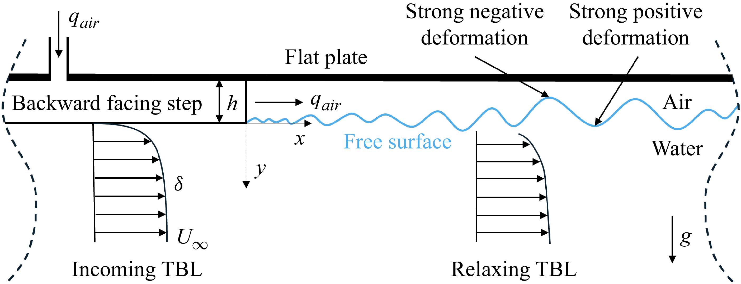

 qair≈60
 U∞=1.2
 tAL=
 U∞=3.6
 tAL=
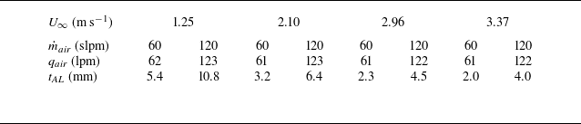
 U∞
 m˙air=60

 (x,y)=(0,0)
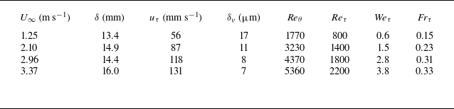
 x=−20
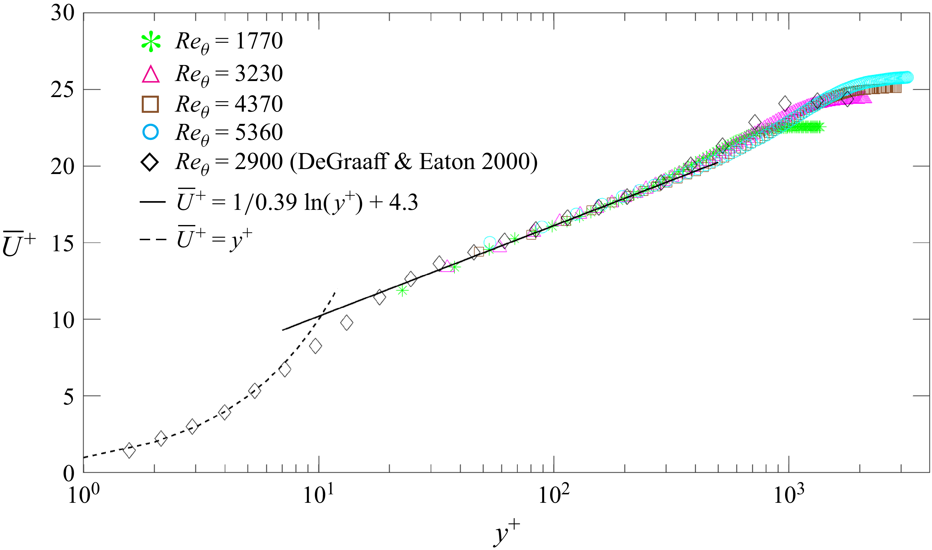
 x=−20mm

 Weτ=0.6,1.5,2.8,
 3.8
 Frτ=0.15,0.23,0.31,
 0.33
 m˙air=60
 100

 d(x,t)
 x=146
 m˙air=60
 Weτ=0.6
 Frτ=0.15
 Weτ=2.8
 Frτ=0.31
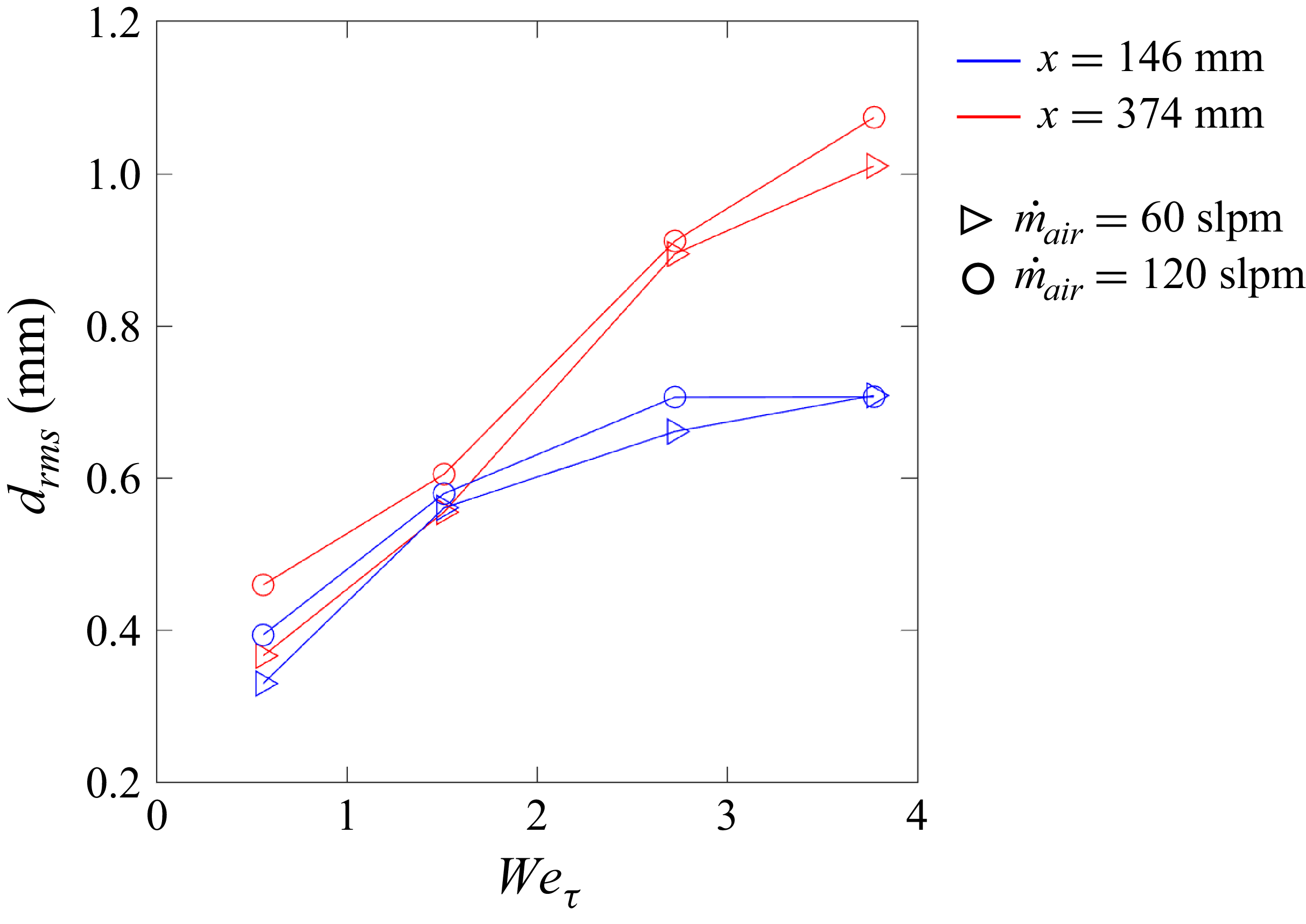
 drms
 Weτ
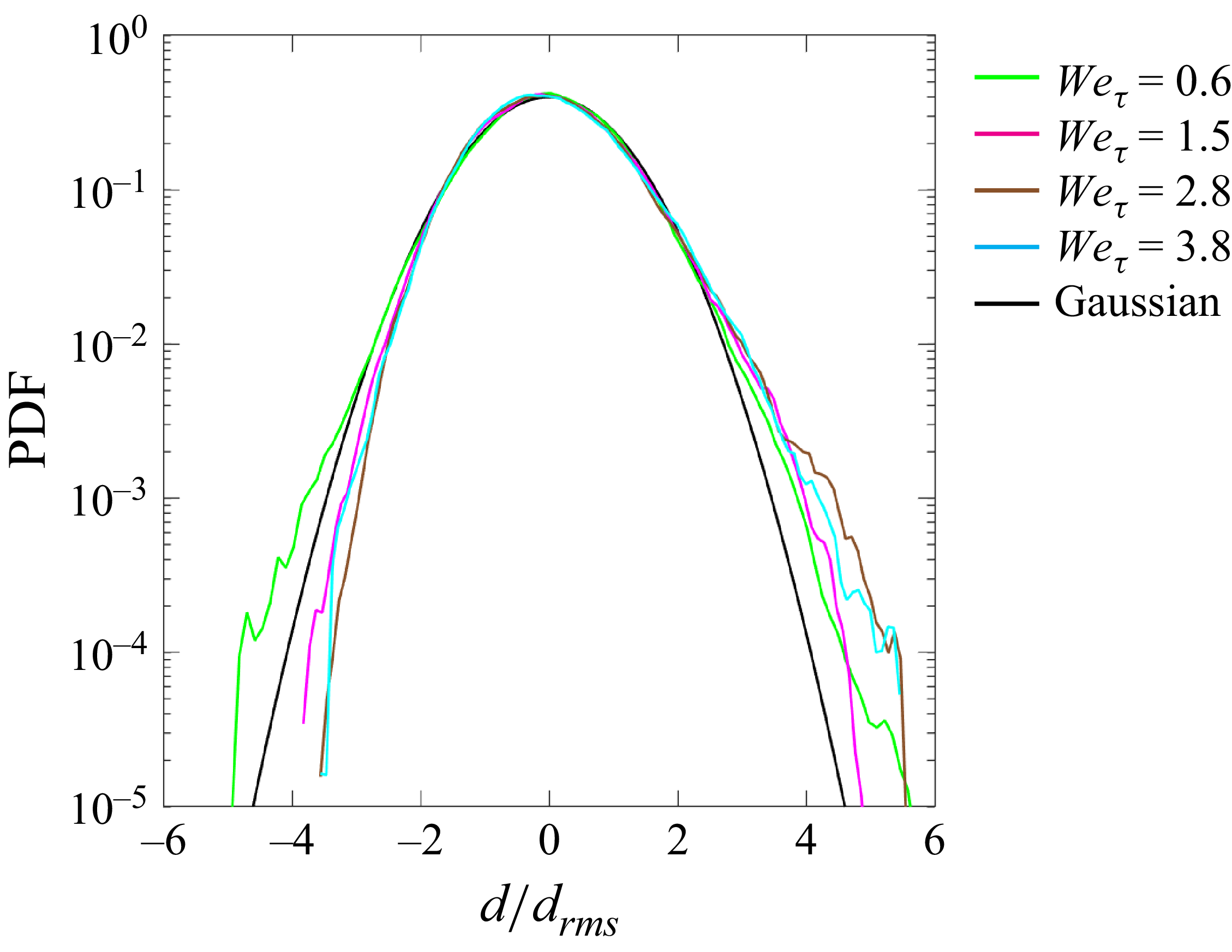
 d/drms
 Weτ
 x=146
 m˙air=60
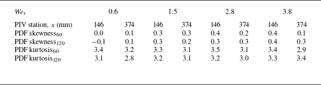

 ϕdd(k,ω)
 Weτ
 Uc
 x=146
 m˙air=60
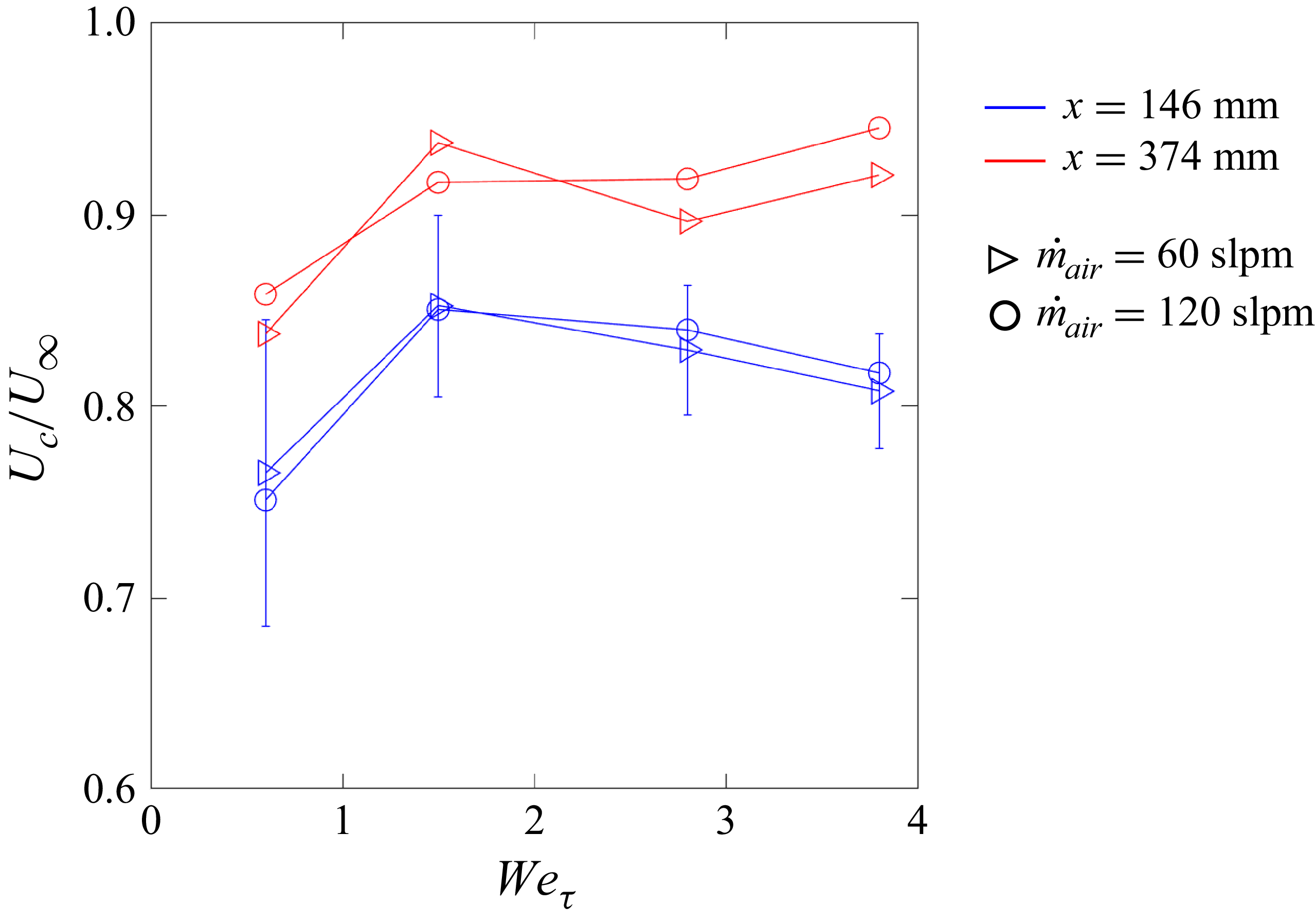
 Uc/U∞
 Weτ
 Weτ
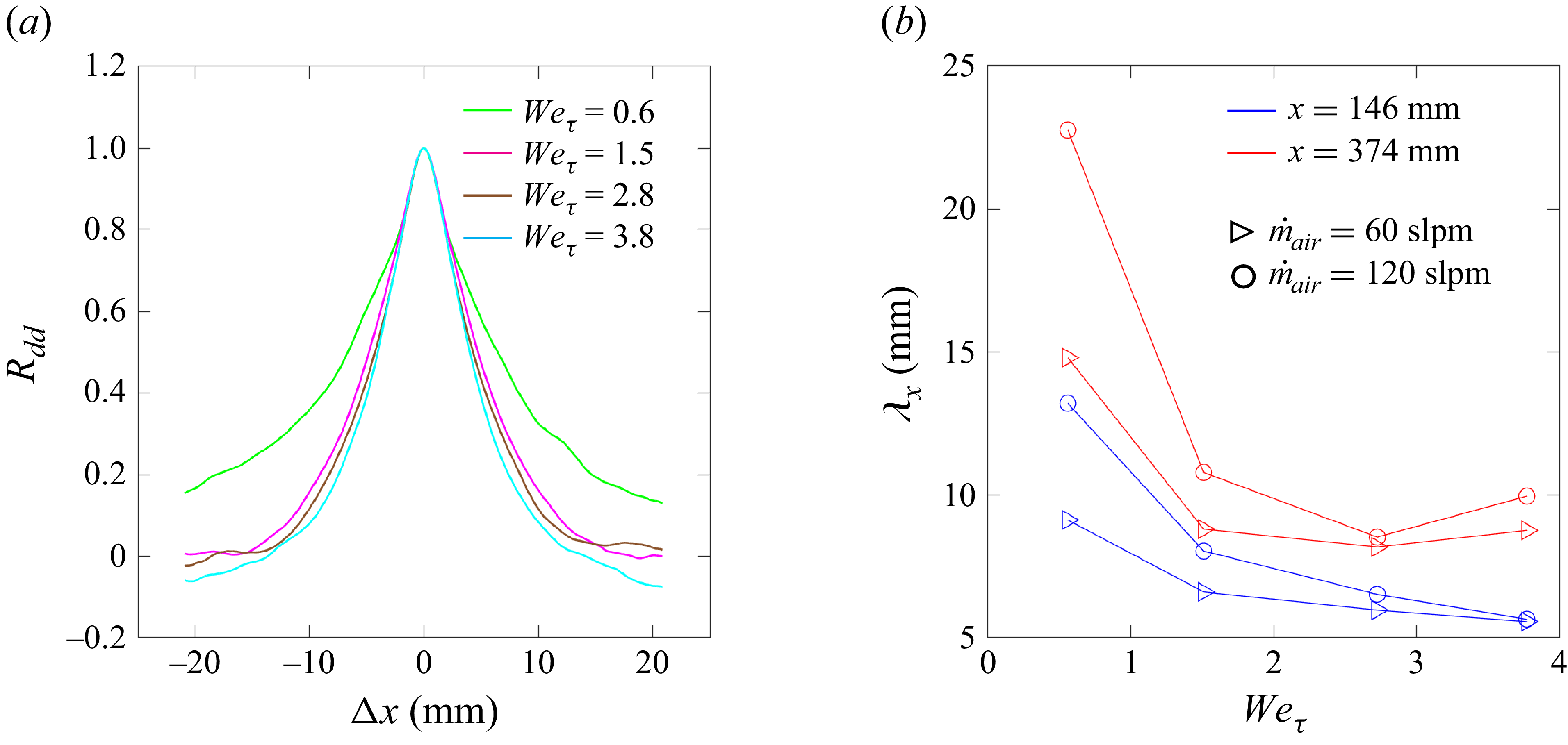
 Rdd
 Weτ
 x=146
 m˙air=60
 λx
 Weτ

 Reτ
 y=0.2δ
 m˙air=60

 Ruu
 y0/δ≈0.6
 Reτ=800
 Reτ=1800
 x=−6
 m˙air=60

 Rvv
 y0/δ≈0.6
 Reτ=800
 Reτ=1800
 x=−6
 m˙air=60
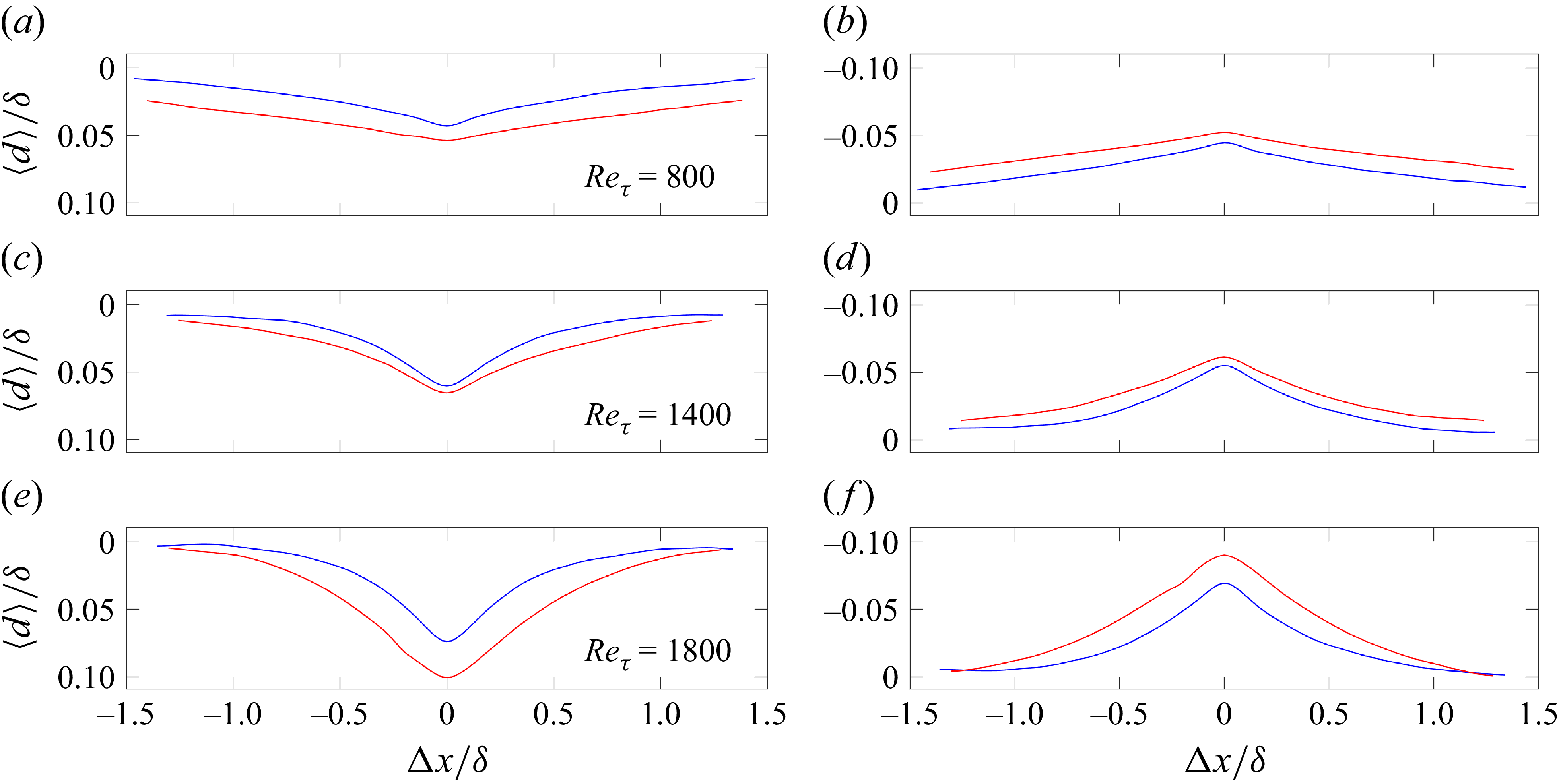
 ⟨d⟩
 Reτ=800
 Reτ=1400
 Reτ=1800
 d>σd
 d<−σd
 x=146
 x=374
 m˙air=120

 ⟨Rdu⟩
 Reτ=800
 x=146
 x=
 m˙air=

 ⟨Rdu⟩
 Reτ=1400
 x=146
 x=
 m˙air=

 ⟨Rdu⟩
 Reτ=1800
 x=146
 x=
 m˙air=


 Open access

