Collective pensions without a sponsor guarantee are becoming increasingly common in the occupational pension sphere. Under these plans, the plan sponsor's commitment is limited to contributions at a specific level or within a predefined range. Plan members, including those still working and those who already retired, pool their assets and liabilities and bear risk collectively. In many cases, the plan has a targeted benefit level or aspiration, but actual benefits may vary from this target due to economic or demographic experience. The target may be defined in nominal or real terms and may be strongly or weakly funded.Footnote 1
Examples of such plans include target benefit plans and shared risk plans in Canada (e.g., Munnell and Sass, Reference Munnell and Sass2013; Wang et al., Reference Wang, Lu and Sanders2018), collective defined contribution (CDC) plans in the UK, and most collective plans in the Netherlands (e.g., Kortleve, Reference Kortleve2013; Bovenberg et al., Reference Bovenberg, Mehlkopf, Nijman, Mitchell and Shea2016). The Dutch plans are classified as either CDC or defined benefit (DB) without a hard guarantee. In all cases, indexation of benefits (if offered at all) is conditional on the financial position of the plan, and accrued benefits must be cut if the funded position is weak and additional assets cannot be secured. In this study, we use the term CDC to describe these types of plans.
In a world of dwindling sponsor guarantees, these plans are seen as a desirable alternative to individual defined contribution (DC) plans, and rightly so: the risk-reducing benefits of collective pensions with risk-sharing elements are well documented in the literature, including Bovenberg et al. (Reference Bovenberg, Koijen, Nijman and Teulings2007), Gollier (Reference Gollier2008), Beetsma and Bovenberg (Reference Beetsma and Bovenberg2009), Blommestein et al. (Reference Blommestein, Kortleve and Yermo2009), Cui et al. (Reference Cui, De Jong and Ponds2011), Beetsma et al. (Reference Beetsma, Romp and Vos2012), and Boes and Siegmann (Reference Boes and Siegmann2018). On the asset side, collective pools tend to create economies of scale that have been shown to improve members' outcomes (e.g., Bikker and De Dreu, Reference Bikker and De Dreu2009; Dyck and Pomorski, Reference Dyck and Pomorski2011; Bikker, Reference Bikker2017). On the liability side, temporary subsidies among generations can create stability without sacrificing expected benefit levels; this enhances utility when members are risk averse (e.g., Gordon and Varian, Reference Gordon and Varian1988; Shiller, Reference Shiller1999; Weil, Reference Weil2008; Westerhout, Reference Westerhout2011).
As noted by Bovenberg et al. (Reference Bovenberg, Koijen, Nijman and Teulings2007), one disadvantage of risk-sharing designs is that intertemporal smoothing may lead to persistent intergenerational value transfers when shocks are spread out over more than the individual's remaining lifetime. Therefore, it is essential to consider the fairness and intergenerational wealth redistribution effect of collective pension schemes. From an ex ante perspective, a pension plan can be fair if the market value of contributions paid throughout one's life is equal to the market value of benefits received during the years in retirement. Cui et al. (Reference Cui, De Jong and Ponds2011) argued that well-structured intergenerational risk-sharing could be a positive-sum game from a welfare perspective, although it is a zero-sum game in market value terms. They concluded that collective pension schemes could be welfare improving over the optimal individual life-cycle benchmark, and the expected welfare gain of the current entry cohort does not come at the expense of older and future cohorts, from an ex ante perspective.
Evaluation of fairness must take into account all risk transactions within the plan. This includes those that are explicit—that is, arising from stabilization mechanisms that are easily visible to stakeholders—such as countercyclical buffers and contingency reserves. It also includes those that are implicit and, therefore, more difficult to notice or assess, such as the change in the valuation rate, for instance. In practice, the focus tends to be on the fairness of explicit stabilization mechanisms. One of our goals is to increase awareness of the implicit risk transactions and to re-evaluate explicit mechanisms in light of these.
Our conceptual model for a generic CDC plan draws on the work of the Canadian Institute of Actuaries' Task Force on Target Benefit Plans (CIA, 2015b), which identified the following five key elements: the contribution rate, the target benefit, the affordability test, the triggers, and the actions.
The contribution rate is the first design element to be set by the CDC plan sponsors. It can be expressed as a dollar amount or a percentage of the member's salary. In most cases, the contributions paid by the plan sponsors are determined at plan inception and fixed thereafter. In some plans, the contribution rate is adjustable to help balance the plan's funding position; however, such adjustments are restricted to a limited range. The contribution rate and funds available at plan inception constitute the total funding resources of the plan.
The target benefit is the benefit that the plan is aspiring to provide; unlike in DB plans, this benefit is not guaranteed. The target is usually defined in a way that is similar to DB plan benefits, for example, a fixed percentage of career or final average earnings multiplied by the member's years of service. Although the actual benefits received by the plan members vary with plan experience, the target benefit acts as a guidepost, allowing members to estimate their retirement income. The target benefit must be consistent with the chosen contribution rate so that there can be a reasonable expectation ex ante of the target being achieved.
The affordability test is performed at each valuation to determine whether the target benefits are affordable. The result of the test is usually expressed as a funded ratio, equal to a measure of plan assets divided by the pension liabilities. Whether the target benefits appear to be affordable will depend on the choice of assumptions and methods used to value the plan's assets and liabilities.
The triggers are used to determine whether the plan's trustees should take some action given the results of the affordability test. In the case of a pure CDC plan, there is only a single trigger, such that whenever the funded ratio deviates from 100%, action is taken immediately to remedy it. In this case, there is very limited risk-sharing among different generations, and the actual benefits may be nearly as volatile as in individual DC plans. To stabilize the retirement income, a lower and upper trigger can be set, forming a corridor within which no action is taken: in this case, the actual benefit will only be adjusted once the funded ratio hits either the lower or the upper trigger. Under such designs, when the plan performs better than expected, part of the surplus may be paid out as benefit improvements, but the rest of the surplus is saved to build a buffer to protect benefits during adverse conditions. This double-trigger design is an example of an explicit benefit stabilization mechanism.
Finally, the actions are the changes that should be made when the triggers are hit. There are several options, which include adjusting the benefits (with respect to past or future service, or both), adjusting the contributions (in plans where the contribution rate is adjustable within a limited range), or changing the investment strategy (e.g., updating the asset allocation).
The first two elements (i.e., the contribution rate and the target benefit) determine the plan cost and the funds available, while the last three (the affordability test, triggers and actions) control the risk-sharing structure. Different design choices and assumption sets have an impact on the risk transactions among members and can significantly change the distribution of the pension benefits payable to different cohorts. We start by comparing the distribution of benefits under a pure CDC plan against the corresponding distribution under an individual DC plan benchmark to isolate any implicit risk transactions. We then explore the impact of additional design elements.
The foundation of our investigation is to use derivative pricing techniques to value contingent claims within the pension fund. Kocken (Reference Kocken2006) studied embedded options in DB plans with conditional indexation and in pure CDC plans. The pension plan modelled by Kocken (Reference Kocken2006) was straightforward: the membership was reduced to two groups of participants (actives and retirees), and the retirement benefits were assumed to be paid out through two lump-sum payments.
Hoevenaars and Ponds (Reference Hoevenaars and Ponds2008) extended the work of Kocken (Reference Kocken2006) by considering each individual cohort instead of the two broad membership groups. Their approach, based on Ponds’ (Reference Ponds2003) valued-based asset and liability management (ALM), is a combination of stochastic projections, generational accounting and derivative pricing techniques. The plan's operation is projected using Monte Carlo simulation, and the real-world cash flows are recorded separately for each generation. The market-consistent value of the pension contract for each generation is then evaluated using risk-neutral valuation.
We apply the value-based ALM method as implemented by Hoevenaars and Ponds (Reference Hoevenaars and Ponds2008) to a pure CDC plan without any explicit stabilization mechanisms and find the net market-consistent value of this pension arrangement for each generation. This value can be interpreted as the impact (positive or negative, for each cohort) of moving from an individual DC plan in which there is no risk-sharing to a pure CDC plan and is therefore a measure of the value of the implicit risk transactions. We explore this value further by decomposing it into the amounts corresponding to the upside and downside risks. We also differentiate between the value derived from benefits received while the plan is ongoing versus the value attached to any residual assets to which a cohort might be entitled at the end of our projection horizon when the plan is assumed to terminate. Finally, we repeat our calculations for CDC plans with alternative implicit and explicit design elements, including one that uses a different discount rate for valuing plan liabilities, and two others with explicit benefit-stabilization mechanisms.
The contributions of this study are threefold. First, the shortcomings of current North American actuarial practice are highlighted in the context of a pure CDC plan with a single benefit adjustment factor. Specifically, we report that non-negligible value transfers are present among different cohorts, and these transfers stem from (1) the use of a single valuation rate based on the actuary's estimate of the expected return on assets (EROA) and (2) the risk-sharing that arises from the use of a single benefit adjustment factor. These transfers are implicit as the pure CDC plan does not have any explicit benefit-smoothing mechanisms. Second, we assess the impact of changing the valuation rate to a single bond-based rate—a common alternative—and report that it does not make the deal entirely fair for all generations from an ex ante perspective. Third, we investigate explicit stabilization mechanisms involving two triggers and a no-action range—so-called corridors. This feature reduces the volatility of retirement benefits without triggering significant additional value transfers if the corridor is symmetric, whereas plans with designs that are biased towards savings tend to shift value from older to younger generations.
The remainder of the paper is organized as follows. Section 1 presents the economic framework used in this study. The structure of the generic CDC plan is described in Section 2. Section 3 discusses the use of derivative pricing techniques to price embedded options. Intergenerational transfers are assessed in Section 4. Then, Section 5 is devoted to the introduction of explicit stabilization mechanisms in the generic CDC plan. Section 6 investigates the CDC plans—with and without explicit stabilization mechanism—from a utility theory perspective. Some robustness tests are presented in Section 7. Finally, Section 8 concludes.
1. Economic and financial framework
An economic scenario generator (ESG) is required to make stochastic projections. It can be defined under both real-world (physical or P) and risk-neutral (pricing or Q) measures. The real-world version of the ESG focuses on expressing a particular future view of the economy, and it enables us to investigate how the pension plans would perform under specific future economic conditions. By contrast, the risk-neutral version of the ESG is used to consistently evaluate contingent cash flows, whose values depend on the stochastic economic variables. Since we are interested in both the possible future outcomes and the value of intergenerational transfers under different plan designs, we need to construct an ESG that is capable of simultaneously handling both real-world and risk-neutral measures.
In this study, we use a model that combines the first-order vector autoregressive model, that is, VAR(1), and the generalized autoregressive conditional heteroskedasticity model, or GARCH(1,1). The mean reversion feature and the autocorrelation among the economic variables are captured by the VAR(1) model—similar to that used by Hoevenaars and Ponds (Reference Hoevenaars and Ponds2008). In addition, the constant volatility in the VAR(1) model is replaced by a more realistic time-varying volatility, which is modelled by GARCH(1,1) processes. We also allow for a general correlation structure between the different noise terms in the spirit of Escobar et al. (Reference Escobar, Rastegari and Stentoft2019). For more details, see Appendix A.
A corresponding risk-neutral version of our VAR-GARCH model can be derived by assuming that the time-varying risk premiums are affine functions of the economic state variables. This risk-neutral model is consistent with the stochastic discount factor (SDF) approach used in Hoevenaars and Ponds (Reference Hoevenaars and Ponds2008). Further details on the risk-neutralized version of the model are available in Appendix A.
This study considers four key economic variables. Let $r_n^s$ and $r_n^l$
 be the monthly nominal yield of a short-term bond and of a long-term bond at the beginning of month n, respectively. Additionally, let i n be the monthly inflation rate applicable during month n, and r n be the monthly S&P/TSX composite index (log) return cum-dividend in excess of the short rate (i.e., $r_n^s$
 ).
Canadian economic data from May 1991 to December 2018 are used. Further details on the datasets can be found in Appendix B.Footnote 2 To find the model parameters, we conduct a two-stage estimation procedure for the ESG. In the first step, the VAR-GARCH model real-world parameters are estimated using maximum likelihood estimation. In the second step, the risk premium parameters $ {\bi\lambda}_0 $ and $ {\bi\lambda}_1 $
 are calibrated, conditional on the real-world VAR-GARCH parameters, by minimizing the sum of the squared differences between the historical zero-coupon yields and the model zero-coupon bond yields calculated from the Q measure using Monte Carlo simulation. This two-stage estimation procedure is consistent with the approach used by Hoevenaars and Ponds (Reference Hoevenaars and Ponds2008). Additional details regarding the estimation are available in Appendix C.
2. Stylized plan and key features
We construct several variants of the generic CDC design and simulate their operation under the various economic scenarios generated by the processes described in Section 1.
Before the inception of the CDC plan, members are assumed to have had individual DC accounts in which they accumulated assets while employed and from which they drew assets once retired. The individual DC account balances of all members (active and retired) are transferred into the CDC plan and commingled at inception. The pension fund is liquidated after 100 years, and all the remaining assets are distributed to the participants as a lump-sum payment at t = 100 based on predefined entitlement criteria.
Plan membership is stationary, with 100 new members entering the plan each year at age 30, retiring at age 65, and dying at age 86.Footnote 3 There are no decrements before age 86, so there are 56 cohorts of precisely 100 members each at all times.Footnote 4 Moreover, participation is mandatory.
Salaries increase at the beginning of each year. The growth rate applicable in year t consists of the annual inflation rate in year t, $\tilde{i}_t$ , and a fixed annual increase for promotion and merit, m = 0.5%.Footnote 5 The starting salary of the new entrants at time zero is $50,000. The salaries of subsequent cohorts of new entrants are the same in inflation-adjusted terms. All active members contribute at the same fixed rate c of 4.7% of salary, payable at the beginning of each year. The total contributions made to the plan at time t are denoted by C t.
The target benefit TB x,t at time t of an active member aged x is based on a final-pay formula

where the target annual accrual rate b t applies to all service (i.e., past and future). The projected final salary PFS x,t is the salary that a member aged x at time t is projected to earn in his final year of employment (i.e., just before retirement). The salary is projected under the assumption of a constant future inflation rate of 2%. Retirement benefits B x,t are paid to a retiree aged x at the beginning of year t based on the current target accrual rate and each retired member's actual final-year earnings S 64,t−(x−64), without indexation after retirement. The value of retirement benefits B x,t can be expressed as

When the target accrual rate is adjusted, the benefits of all members, including retired members, change. The total benefits paid from the plan at time t are $B_t = \mathop \sum \nolimits_{x = 65}^{85} 100B_{x, t}$ .
The initial target accrual rate b 0 is set to 1%. A test is performed at the beginning of each year, before contributions are received and benefit payments are made, to decide whether the target accrual rate determined in the previous valuation is still affordable. Given the availability of funds and the future contribution commitment, two crucial elements will affect the result of this affordability test: the valuation assumptions and the valuation method used to evaluate the plan assets and liabilities.
For the plan assets, we assume that half of the fund is invested in equities modelled in Section 1 and the rest is invested in a rolling portfolio of 15-year zero-coupon bonds, rebalanced annually. Annual effective returns for each asset and for the combined portfolio are obtained directly from the simulation results of the VAR-GARCH model.Footnote 6 The annual portfolio return in year t—a by-product of the ESG—is denoted by $r_t^P$ . The value of the plan assets F t can be expressed recursively as

The assumptions needed to value the plan liabilities relate to mortality, future salary increases, and the valuation rate. For purposes of the affordability test, all members are assumed to die at age 86, and salaries are assumed to increase at a fixed annual rate based on a forward-looking inflation assumption of 2% per year and the 0.5% per year increase for merit and promotion. The valuation rate applicable at time t varies with the economic scenarios generated by the processes in Section 1. It may reflect the actuary's (imperfect) estimate of the expected return on the plan assets as of the valuation date, or it can be based on the yield on long-term bonds as of that date.
The actuary's estimate of the EROA is constructed by following the ‘building block approach’ in the guidance material published by the CIA (2015a). We take the yield on 15-year zero-coupon bonds at time t as the actuary's best estimate of the long-term returns expected on the bond portion of the pension fund from time t onwards. To estimate the long-term return on the equity portion of the fund, we add a fixed risk premium to the 15-year zero-coupon bond yield.Footnote 7 We use an equity risk premium of 4.5%, which is consistent with the current risk premium in the economy (Graham and Harvey, Reference Graham and Harvey2018). Therefore, the valuation rate based on EROA is $\tilde{r}_t^l + 1/2$ (0.045), where $\tilde{r}_t^l$
 is the long-term bond yield, expressed as an effective annual rate and derived from the ESG outputs.Footnote 8
Plan liabilities are determined using the Entry Age Normal cost method as described in Aitken (Reference Aitken1996). We chose this method because it is consistent with a level contribution rate applied throughout a member's working life, and therefore avoids the intergenerational cost subsidies that arise when benefit allocation-type cost methods (e.g., unit credit) are combined with a uniform contribution rate. Under the Entry Age Normal method, the actuarial liability with respect to each member is equal to the present value of the member's projected benefits less the present value of their future normal costs. The normal cost is calculated as the level per cent of salary that is required to finance the targeted benefit over the member's entire working life, from entry to retirement. The actuarial liability of the plan at time t, L t, is the sum of the individual liabilities. Note that, for purposes of the affordability test performed at time t > 0, the members' projected future benefits are first determined using the target accrual rate b t−1 established at the previous valuation. Therefore, L t is based on b t−1. The key output of the affordability test is the funded ratio FR t = F t/L t.
The initial target accrual rate b 0 is consistent with the contribution rate c in the sense that the normal cost established under the Entry Age Normal method with respect to this target is 4.8% when using a valuation rate equal to the actuary's best estimate (i.e., EROA) at plan inception. The benefit accrual rate may be adjusted at subsequent valuation dates according to pre-specified rules in the pension contract based on the result of the affordability test. In a pure CDC plan, there is only a single trigger point set to a funded ratio of 100%. Under this plan design, whenever the funded ratio determined by the affordability test is not equal to 100%, actions are taken immediately. Specifically, at each time t > 0, the new accrual rate b t is determined by multiplying the accrual rate b t−1 established in the previous valuation by a factor $ \alpha _t $ . For the pure CDC plan, we implement the following adjustment factor:

where PVTB t is the present value of the targeted benefits with respect to both past and future service for active and retired members, and PVFNC t is the present value of future normal costs for active members, both based on the most recent target accrual rate, b t−1. This factor returns the funded ratio after adjustment to exactly 100% by construction.
As noted above, using a single trigger leads to highly volatile retirement benefits. Plan stakeholders may wish to add an explicit benefit stabilization mechanism with a double trigger and a no-action range between the trigger points. We study in Section 5 two plan designs with such explicit stabilization mechanisms. In the first one, the no-action range is set symmetrically around a funded ratio of 100%. In the second, the no-action range is biased towards savings, with the lower bound set at a funded ratio of 100%. In both cases, when either the lower or upper trigger is hit, the target accrual rate is adjusted to bring the funded ratio back to the edge of the no-action range.
The starting asset value at the inception of the CDC plan F 0 is the sum of members' individual DC account balances. We assume that each member's individual account balance is precisely equal to that member's Entry Age Normal liability calculated using a valuation rate equal to the EROA. This means that, when the affordability test is performed at plan inception, the funded ratio will be exactly 100% as long as the valuation rate used in the affordability test is also equal to the EROA. If, on the other hand, the affordability test uses a valuation interest rate based on the long-term bond yield applicable at time zero, the funded ratio will differ from 100%, and the initial target accrual rate b 0 will need to be modified.
3. Quantifying risk transactions using derivative techniques
In this section, our goal is to quantify the risk transactions within the stylized CDC plans described in Section 2. We follow the value-based ALM methodology implemented by Hoevenaars and Ponds (Reference Hoevenaars and Ponds2008) and first determine the cash flows with respect to each cohort. These cash flows fall into four categories: the individual DC plan account values transferred at the inception of the CDC plan, the contributions made while the CDC plan is ongoing, the benefits received from the CDC plan while it is ongoing, and the residual assets distributed to members when the plan is terminated.Footnote 9
These cash flows can be constructed under both real-world and risk-neutral scenarios. The real-world cash flows reflect the contribution and benefit payments that the plan member would expect under possible economic conditions in the future. The cash flows calculated under the risk-neutral scenarios are not meaningful in themselves; however, they enable us to calculate the market-consistent value of the pension deal for each generation at time zero and to investigate the gains and losses of each generation arising from their participation in the CDC plan.
From these cash flows, we compute the generational value of the pension deal as the risk-neutral expected present value, at plan inception, of all cash flows of a specific cohort.Footnote 10 Specifically,
• The retirees at the inception of the plan start receiving their retirement benefits immediately after inception. Their pension value is equal to the value of the benefits they have yet to receive minus the funds they bring into the plan at inception.
• For active members at plan inception, the value of the deal is equal to the value of the retirement benefits they will receive net of the value of the funds they bring into the CDC plan and all their future contributions.
• The generations that are not yet in the plan at inception but that are already dead when the plan is terminated will receive their benefits in exchange for their contributions. The value of their pension deal does not include any residual payout.
• For the members who are still in the plan 100 years after its inception, the value of the pension deal includes the value of the actual retirement benefits and the residual payout they will receive, less the value of the contributions they will make.
More details on the technical derivations of the generational values are given in Appendix D.
While changes in the generational value from design to design reveal shifts in the overall risk profile of each cohort, it is useful to explore these shifts at a more granular level, distinguishing between changes in upside versus downside risks, and between risks associated with the ongoing benefits versus risks associated with the residual payments. We, therefore, also decompose the cash flows under each CDC design into the corresponding cash flows under an individual DC plan benchmark and any additional (positive or negative) cash flows.
If the starting account balances and subsequent contributions are the same under the individual DC benchmark as they are under the CDC plan and both plans enjoy the same portfolio returns, then the additional cash flows must relate to differences in the benefit payments and the residual values. These differences occur because the CDC plan adjusts the benefits of each member with reference to the experience of the whole plan, whereas adjustments to the payouts from the benchmark plan only reflect the experience of a single individual. Effectively, by joining the CDC plan, the participants write put options to the plan, which waive part of the benefits they would have obtained in the individual DC plan. In exchange, participants are offered call options written on the fund surplus. The same applies to the residual asset under the CDC plan: it can be thought of as the residual asset under the individual DC plan plus a put option written by members and a call option received by members. This yields four kinds of options: a benefit put option, a benefit call option, a residual put option, and a residual call option. More details on each of these options are given in Appendix D.
The total generational value is computed as the sum of these four options. As explained in Cui et al. (Reference Cui, De Jong and Ponds2011), the call and put option values can be used to assess the potential for ex post risk: the larger the option values, the more potential for ex post risk—and this is the case even if the total value of the options is nil.
4. Evaluation of CDC schemes
We now turn to evaluating intergenerational transfers under specific CDC designs. We first assess the pure CDC plan. Specifically, we appraise the performance of the plan and compute the market value of the pension deals. Then, we investigate alternative affordability tests, that is, different valuation rates and their impact on redistribution.
4.1 The pure CDC plan
We first consider a pure CDC plan—our base case—where the valuation rate used in the affordability test is closely tied to the actuary's best estimate, based on the EROA.
The initial target annual accrual rate b 0 is 1%. No immediate benefit adjustment is needed at time 0 because the funded ratio produced by the affordability test is precisely 100% by construction (i.e., the target accrual rate is consistent with the combination of the starting asset value F 0, the contribution rate c, and the valuation basis).
Since half of the plan assets are invested in the stock market, which earns the equity risk premium in the long run, the EROA valuation rate should be close to the actual investment return, on average. The median spread between the simulated asset return and the simulated valuation rate hovers around 0% each year, indicating that the fund is as likely to experience investment gains as losses.
We make a few observations about the performance of the plan using some of the metrics considered by Sanders (Reference Sanders2016) before turning to the value-based ALM framework. The distribution of the funded ratio of this plan is quite steady over time; Figure 1 reports the funnel of doubt of the funded ratio distribution over the next 100 years. The median is 100% at time zero and remains there until the last payment is made. The funnel of doubt is rather narrow around this median value, with 2.5th and 97.5th percentiles of 0.87 and 1.23, respectively.
Funnel of doubt of the funded ratio for the pure CDC plan.
Notes: The funded ratio of the pure CDC plan before the adjustment is calculated at each valuation date for the base plan. The 2.5th, 25th, 50th, 75th, and 97.5th percentiles of the simulated distribution of the funded ratio are shown.

Pensioners do not want their retirement benefits to fluctuate every year. However, since the pure CDC plan has a single trigger, the benefits are not very stable: Figure 2 depicts the distribution of benefit adjustments by size at each valuation date. Specifically, it reports that the probability of increasing or decreasing the benefit drastically (i.e., by more than 5% in absolute value) in any given year is quite high—approximately 50%. Throughout the projection period, the likelihood of negative adjustments is somewhat similar to that of positive adjustments.
Distribution of benefit adjustments by valuation year for the pure CDC plan.
Notes: The distribution of the size of the benefit adjustments is calculated at each valuation date for the pure CDC plan. Each bar in the figure summarizes the distribution for a given year.

This pattern can also be observed when computing the annual replacement ratio, which attempts to capture the cumulative impact of the adjustments over the lifetime of a member. In fact, the distribution of the replacement ratio is very steady over the 100-year period: the median of the replacement ratio settles near 55%.
In practical settings, the distribution of funded ratios, benefit adjustment factors, or replacement ratios under the physical measure may be used by stakeholders to assess intergenerational equity. We felt it was important to point out that even though the pure CDC design considered here (including the specific valuation framework and the benefit adjustment mechanism) appears to be fair in these respects, it might not be so in risk-adjusted terms. We use the value-based ALM framework to shed light on the intergeneration value transfers in terms of the market-consistent value. Figure 3 shows the generational pension value for different cohorts under the pure CDC plan calculated as explained in Section 3. The values on the x-axis represent the ages at plan inception of the various cohorts who enter the plan. Since the value of the pension deal is defined as the market value of all payouts minus all contributions, a pension value of zero represents a fair deal without any value transfers at plan inception.Footnote 11
Pension deal value for the pure CDC plan.
Notes: The value of the pension deal is calculated using Equation (9) for all the generations who enter the plan before its termination. The x-axis in the figure shows all the cohorts of members, with negative numbers representing the cohorts who are not yet born at plan inception.

In Figure 3, the value of the pension deal for generations who are older than 44 at inception is positive, meaning that these cohorts are expected to be net winners if they enter this pure CDC plan. By contrast, the other generations (i.e., those less than age 44 at inception, including those not yet born) can expect to be net losers, on an ex ante basis. Without access to any external funding sources—as it is the case here—the pension deal is a zero-sum game in market value terms, so one cohort's gain comes at the expense of other cohorts. Specifically, the cohort that is worst off (those around age 25 at plan inception) loses nearly $8,300 in value (17% of their salary at inception), whereas the cohort that is best off gains approximately $15,400. In sum, although this plan does not have explicit risk-sharing, Figure 3 draws attention to the implicit risk-sharing structure of the pure CDC plan.
This result—non-zero pension deal values—is evidently in opposition to Cui et al.'s (Reference Cui, De Jong and Ponds2011) main result. In the latter, the authors set up a plan in such a way that it is always fair from an ex ante standpoint. Specifically, they select the sharing rules such that the contribution and benefit levels' risk-neutral expectations are equal to their targets. We note that, when converted to the physical measure, their approach gives rise to benefits that drift upwards over time, even though these benefits are a martingale under the risk-neutral measure by construction (see Figure 2 of Cui et al., Reference Cui, De Jong and Ponds2011).Footnote 12
By contrast, in our study, the real-life inspired sharing rules are set up with the intention of keeping the expected value of the benefit accrual rate more or less constant in the real world. This reflects the desire of stakeholders to maintain a level expected replacement ratio over time. However, due to the presence of a positive equity risk premium in the real world and its absence in the risk-neutral world, the constant expected benefit accrual rates in the real world translate into a decreasing pattern of expected benefit accrual rates in the risk-neutral world. This favours older members at plan inception who are expected to receive higher benefits in risk-adjusted terms than the cohorts that follow. The pattern shifts after about 15 years and the expected benefit accrual rate under the risk-neutral measure eventually stabilizes.
Figure 4 reports the value of the options embedded in the pure CDC plan for all cohorts. The benefit option plot (top panel) indicates that most cohorts that are currently in the plan—between 30 and 86 years old at inception—have significant upside potential as measured by the value of the benefit call options (VTBC): up to $21,000 in market value terms. This upside comes at the expense of the future generations, who have significant downside potential, as measured by the value of their benefit put options (VTBP).
Embedded options for the pure CDC plan.
Notes: The value of the embedded options is calculated for all generations who enter the plan before its termination. The figure on the top shows the generational values of VTBP and VTBC calculated using Equations (12) and (13), respectively. The figure in the middle shows the generational values of VRP and VRC calculated using Equations (10) and (11), respectively. The figure at the bottom shows the total value of the call options and the put options for each generation.

The price of the options in the top panel of Figure 4 also informs us of the size of the ex post transfers, as explained in Ponds (Reference Ponds2003). There is potential for large (positive) ex post transfers to older generations, whereas the transfers would possibly only be modest (and negative) for current active members and future cohorts.
The middle panel of Figure 4 reports the value of the residual call and put options (VRC and VRP, respectively), which are small for most cohorts: up to $3,000 in market value terms. The long simulation horizon might explain this, to some extent.
Finally, the bottom panel of Figure 4 shows the aggregate value of the surplus and deficit options from the first two plots. Since the value of the individual DC plan is equal to zero for each generation, the value of the pension deal for each cohort is equal to the total value of the call options of that cohort less the total value of the put options for the same cohort.
4.2 On the reasons behind non-zero value transfers
Although there are no explicit intergenerational risk-sharing mechanisms built into this plan design, value transfers between different cohorts still exist. There are two reasons for this: (1) the pricing of benefits on an actuarial rather than risk-adjusted basis at each valuation date and (2) the implicit sharing of the liability-side gains and losses among all members.
The impact of the naive pricing of benefits for purposes of the annual affordability test is both significant and persistent. As described in Section 2, the contribution rate is calibrated by the actuary at inception using a target benefit rate of 1%. However, instead of equating the risk-adjusted expected values of the contributions and benefits as in Cui et al. (Reference Cui, De Jong and Ponds2011), the present value of the contributions received during a member's working life is set to be equal to the present value of the targeted benefits under a single deterministic scenario using the actuary's estimate of expected future returns. Similarly, the starting asset value is set to be equal to the actuarial liability determined using the same methodology. This approach reflects current actuarial practice but misprices the targeted benefits in risk-adjusted terms. Specifically, it undervalues both the risk-adjusted liability and the risk-adjusted future cost of benefits at plan inception by replacing the distribution of possible future returns with a single value and by treating the expected equity risk premium as certain to materialize. As a result, members in the early years receive more than their ‘fair share’ of benefits. The mispricing continues at each new valuation date, although its size and direction change over time due to the dynamics of our ESG.
The second design feature contributing to the value transfers is the single adjustment factor that is applied to all members' benefits in respect of both past and future service. Under the pure CDC plan, this adjustment factor is equal to the funded ratio; benefits are increased (decreased) whenever there is a gain (loss) relative to the actuary's assumptions made in the previous valuation. Gains and losses can arise from both the asset and liability side. Since each member's asset share is invested the same way, it is reasonable that asset side gains should affect members' benefits in equal proportion. However, not all members contribute to the gain or loss in the same proportion on the liability side.
Our model admits liability-side gains or losses from three sources: a discrepancy between assumed and actual inflation, a change in the actuary's valuation rate (tied to the long bond yield), or a discrepancy between the contribution rate established at inception and the normal cost of benefits.Footnote 13 These gains and losses and their impact on benefits are clearly visible ex post, yet it is not immediately obvious that they should lead to redistribution ex ante: the advantages and disadvantages of implicit risk-sharing may cancel out across possible future economic states or over the life cycle. There are several obstacles to this in our model. First, although the actuary expects gains and losses to cancel out in the cross-section in the physical world, they will not do so under the risk-neutral measure. Second, in our ESG, the market price of risk varies with time; hence, the market price of the benefit-risk faced by a member when young does not necessarily cancel out the market price of the benefit-risk faced by the same member when older.
4.3 The impact of alternative affordability tests
Every fairness assessment performed using the value-based ALM method is extremely sensitive to (1) the population dynamics, (2) the starting point for economic projections (i.e., equilibrium versus non-equilibrium), and (3) the accuracy of the actuary's estimate of the expected equity risk premium—or the valuation rate broadly speaking. We will now focus on the last item.
The relationship between intergenerational equity and key design choices in CDC plans is of great concern to actuaries and other stakeholders. For instance, the pure CDC plan analyzed in Section 4.1 uses the EROA valuation rate (i.e., anticipating the equity risk premium) in the affordability test. However, one area of particular interest and active debate is the choice of valuation rate and its impact on intergenerational equity. Using a valuation rate based on bond yields is a possible alternative to EROA. Recently, Sanders (Reference Sanders2016) investigated the changes in the dynamics of the retirement benefits in simple CDC plans after applying EROA as the valuation rate. Ma (Reference Ma2018) also explored the issue of selecting discount rates for assessing the funded status of the same types of CDC plans and concluded that a valuation rate based on EROA is more equitable and serves the best interests of all members. To test the conclusion of Ma (Reference Ma2018) under our framework, we change the valuation rate to bond-based rates while leaving all other design features unchanged.
Effectively, this change results in an average decrease of approximately 2.3% in the valuation rate, increasing the median spread between the simulated asset return and the simulated valuation rate. Since the initial asset value is unchanged, but the valuation rate is lower, the starting funded ratio will be lower than 100% (see Figure 5). This results in a significant negative benefit adjustment at the first valuation date, which quickly returns the median of the funded ratio to 100%. A significant proportion of the deficit that becomes visible at the first valuation—to which all generations contributed at inception—needs to be paid off indirectly by the members who are already retired via benefit reductions. Furthermore, because the new valuation rate tends to slightly underestimate the investment return in the first few years, retirees pay for a more substantial portion of the deficit. After the first few years, positive and negative benefit adjustments are steadier yet biased towards positive adjustments, as shown in Figure 6.
Funnel of doubt of the funded ratio for the bond-based plan (EROA-implied funding).
Notes: See the description of Figure 1.

Distribution of benefit adjustments by valuation year for the bond-based plan.
Notes: See the description of Figure 2 for further details.

Figure 7 reports the value of the pension deal under this modified plan (i.e., solid black line for the EROA plan in Section 4.1 and dashed grey line for the modified plan). In contrast to the positive pension value under the pure CDC plan in Section 4.1, the members who are already retired at plan inception have a negative market-based pension value when using a bond-based valuation rate. This is because their retirement benefits need to be reduced at first as the plan is in deficit from the initial contributions of both the active and retired members. Those who are still active at plan inception (i.e., who retired after the initial deficit was reduced to zero) are better off because the deficit resulting from the inadequacy of their initial contributions is paid off by the retirees, and the probability of positive benefit adjustments is higher.
Pension deal value for the EROA plan and the bond-based CDC plans.
Notes: See the description of Figure 3 for further details. The solid line represents the generational values under the EROA plan. The dashed grey line corresponds to the bond-based plan that uses the EROA-implied structure, and the dashed black line represents the generational values under the collective DC plan with a bond-based valuation rate while using a fully funded plan at inception and a consistent contribution rate.

Overall, the values are shifted from the older generations to those below age 65 at inception. Most of the benefit loss for older generations comes from the higher likelihood of negative benefit rate adjustments in the early years.
In our first findings, the difference between the retirement benefit dynamics in the EROA case and the bond-based case is inconsistent with Ma (Reference Ma2018). Under our specific model and plan provisions, using the EROA as the valuation rate could not be characterized as ‘more equitable.’ Using the bond-based rate simply shifts benefits from current retirees to active members, but does not bring the ex ante pension deal values closer to zero. In other words, only switching the valuation basis does not make the plan more equitable.
This conclusion is, however, conditional on the fact that the plan starts with a funded ratio below 100%, as implied by the EROA-based contribution rate and initial asset value F 0. If we instead consider a plan entirely based on the bond-based valuation rate, then we have a different picture. However, this would significantly change the initial structure of the plan; it doubles the contribution rate from 4.7% to 8.7% and increases the initial value of the fund by 25%. Figure 7 reports the difference between these two cases (see the dashed black line). With this change, the pension deal values are much more similar to those obtained with the EROA rate, although they are larger in absolute value, generally speaking. This new conclusion seems to be consistent with Ma (Reference Ma2018), meaning that a bond-based valuation rate could create additional intergenerational risk transfers.
5. Introducing explicit stabilization mechanisms
The retirement benefits in the pure CDC plans investigated in the previous sections are adjusted at every valuation date and can fluctuate significantly. Plan designs with two triggers are commonly adopted in practice to add stability to pure CDC plans. There may be a sense among stakeholders that the benefit stability achieved by introducing the no-action range comes at no additional cost. In reality, this stability is made possible by requiring potentially more substantial intergenerational subsidies, which may have hidden costs. In this section, we investigate these subsidies, focusing on ex ante fairness.
5.1 Triggers centred on a funded ratio of 100%
We first add a no-action range for funded ratios between (100 − (y/2))% and (100 + (y/2))% to the plan design in Section 4.1 (i.e., the pure CDC plan with the EROA as the valuation rate), where y/100 is the width of the corridor. Since this range is centred on a funded ratio of 100%, this plan is called a symmetric corridor plan. Under this plan design, benefits are unchanged until the funded ratio moves outside the no-action range, at which point adjustments are made to bring the funded ratio closer to the edge of the range. For example, if the width is 40% and if the funded ratio is 140% at the valuation date, then an adjustment factor is applied to the target accrual rate to bring the funded ratio to 120%.
For these plans, as for the corresponding plan in Section 4.1, the median of the funded ratio starts at a value of 100%: the median funded ratio in the symmetric corridor plan remains at the midpoint of the no-action range.
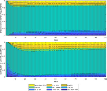
The effectiveness of the no-action range in reducing the frequency and magnitude of benefit changes is demonstrated in the top panel of Figure 8: the benefits remain unchanged from one year to the next with a probability of more than 70% if the width of the corridor is 40%.Footnote 14 The probability of a significant benefit adjustment (i.e., an increase or decrease greater than 5%) occurring in any given year is reduced from 50% to 15% with a corridor width of 40%.
Distribution of benefit adjustments for 40% symmetric and saving corridor plans.
Notes: See the description of Figure 2 for further details. The top panel reports the distributions of benefit adjustments for the symmetric corridor case with a width of 40%. The bottom panel shows the distributions for the saving case with a width of 40%.

The top panel of Figure 9 reports the value of the pension deal under the symmetric corridor plan design for three different corridor widths: 10%, 20%, and 40%. This figure indicates that the no-action range centred on a funded ratio of 100% adds significant stability to the plan without creating value transfers that are too large.Footnote 15 The pension deal value is virtually the same for a corridor width of 10% across all cohorts when compared to the pure CDC plan. It becomes slightly larger (in absolute value) when the width is 20% or 40%. Specifically, if the width is set to 40%, the best cohort gains approximately $25,700 (instead of $15,400 for the pure CDC case) whereas the worst cohort loses approximately $12,500 (instead of $8,300 with the CDC).
Pension deal value for the corridor plans and the pure CDC plan.
Notes: See the description of Figure 3. The top panel reports the value for the symmetric corridor case with widths of 10%, 20%, and 40%. The bottom panel shows the value for the saving case for the same width. The solid black line represents the generational values under the pure CDC plan.

In summary, adding a symmetric corridor to a pure CDC plan is a desirable feature because it makes the distribution of the benefit adjustments more stable over time without substantially altering the value of the pension deal.
5.2 Triggers centred on a funded ratio above 100%
Canadian regulations for CDC plans allow the use of no-action ranges, although not ones centred on 100%. Generally, the regulations require the lower end of the no-action range to start at 100%. In this section, we implement a plan with lower and upper trigger points set at funded ratios of 100% and (100 + y)%, respectively, where y is either 10, 20, or 40. Since the no-action range is deliberately biased towards saving, we call this a saving corridor plan.
Regarding the dynamics of the funded ratio, the first few years form a transitional period during which time the distribution of the funded ratio widens and drifts upwards. The median funded ratio moves from a value of 100% at plan inception to the centre of the no-action range (i.e., (100 + (y/2))%): instead of staying on average at the fully funded level as the symmetric corridor plan does, the saving corridor plan is expected to accumulate additional buffers. As a result, the benefits are less likely to be adjusted upwards and more likely to be adjusted downwards than under the symmetric corridor plan, at least in the early years. This is confirmed by the bottom panel of Figure 8 for which we see the transitional period lasting 15 years in the case when the corridor width is 40%. After the first few years, the probability of the benefits remaining unchanged at a given valuation date is approximately 70% using a corridor width of 40%, which is similar to the symmetric corridor plan. This is because the no-action ranges have the same ‘size’ or ‘span’ in terms of the funded ratio. However, the probability of positive benefit adjustments in later years is slightly higher, and the probability of negative benefit adjustments is slightly lower under the saving corridor plan than under the symmetric corridor plan because positive returns on the surplus tend to spin-off additional gains.
The bottom panel of Figure 9 illustrates the value of the pension deal under the saving corridor plan designs. There is a definite shift in value from older to younger cohorts. In terms of market-consistent values, the young active cohorts at plan inception are expected to have the largest gain equal to nearly $4,000 more than the pure CDC plan if the corridor width is 40%. The generations retiring immediately after plan inception—or close to retirement—have the most extensive losses (approximately $11,300 more than the CDC plan for the widest corridor considered), equivalent to nearly 23% of their final-year earnings. This is because a part of the surplus that would otherwise fund benefit increases is retained in the plan for accumulating a larger buffer. From these results, we can conclude that the benefit stability created by the saving corridor plan comes at someone's expense: in this case, at the expense of older generations.
To conclude this section, the saving corridor increases the value of the pension deal for the current active members and future cohorts at the expense of the older generations by reducing the benefit rate at an early stage. The initial benefit reduction helps to create an additional cushion; this feature is indeed similar to Allen and Gale's (Reference Allen and Gale1997) two-stage approach, that is, intergenerational risk-sharing, followed by intertemporal smoothing (Allen and Gale, Reference Allen and Gale1997: 538).
6. Certainty equivalent values
However, a question remains: even if there are non-zero ex ante risk transfers between the different generations, is it in the best interest of most members to be part of this CDC plan? In other words, even if a member is on the losing hand of the deal (i.e., negative pension deal value), he/she might be better off given his/her preferences. To answer this question, we use utility theory.
We recognize that there is some tension between the risk-neutral valuation used above and utility theory. Nonetheless, they are used for different purposes in this study: the former informs us of the fairness of a pension deal whereas the latter sheds light on the members' preferences.
We represent individual preference ordering with a utility function. Specifically, we use the constant relative risk aversion utility function defined over a single nondurable consumption good. Let p x,t denote the time-t consumption level for a member aged x. The individual's preferences are then defined by

for an individual aged x at inception, where ϕ measures the degree of risk aversion and δ is the subjective discount rate. Throughout the paper, and unless indicated otherwise, we set the subjective discount rate δ equal to 0.04 and the risk aversion parameter ϕ to 5.Footnote 16 To simplify our calculation, we discard the generations that would receive a residual payment at time 100 (i.e., born more than 15 years after plan inception).
Our comparisons are performed on the basis of the certainty equivalent consumption (CEC). This welfare measure gauges the performance of different pension plans and can be computed easily in our setting by solving this equality:

where the left-hand side of the equation is the individual's expected preference.
Figure 10 reports the CECs for all the cohorts, except for those born more than 15 years after plan inception, under both the pure CDC plan (black solid line) and the DC scheme (dotted line). Overall, for all the cohorts considered, the pure CDC yields higher utility making this plan better than the DC one from an individual preference perspective. The difference seems to be quite small for older generations because they only receive a few payments before they die. Nonetheless, this difference grows over time and can be quite significant for current active members and future cohorts. The implicit risk-sharing in the pure CDC plan (e.g., inflation and duration mismatches) makes the benefits less volatile than those of the DC scheme over time, thus increasing the utility gained from joining the CDC plan.
Certainty equivalent consumptions at inception for the corridor plans.
Notes: The CEC is calculated for each generation between −15 and 86 using Equation (1) for the pure CDC plan (solid black line), the DC plan (dotted black line), and the corridor plan with a width of 10% (dashed black line), 20% (solid grey line), and 40% (dashed grey line). The top panel reports the CEC for the symmetric corridor case with widths of 10%, 20%, and 40%. The bottom panel shows the CEC for the saving case for the same width.

Regarding the explicit stabilization mechanisms, the top panel of Figure 10 shows the CEC estimates for all the symmetric corridor plans considered in this study (i.e., widths of 10%, 20%, and 40%). Adding a symmetric corridor seems to increase the CEC for older generations and reduce it for younger generations, generally speaking. Moreover, the impact of the corridor is more noteworthy for wider corridors than narrower corridors. For instance, a 10% symmetric corridor does not seem to substantially change the CEC estimates when compared to the pure CDC—even if it significantly changes the distribution of the benefit adjustments. However, for a 40% symmetric corridor, the CEC is lower than that of the DC plan for younger members. In this case, it seems that the intergenerational risk-sharing is too large and that members would be better off in a DC scheme.
The bottom panel of Figure 10 reports the CEC estimates for the three saving corridor plans considered in this study. The saving corridor increases the CEC estimates for current young active members and future generations as they are less likely to have benefit reductions. Their CECs also grow as a function of the width of the corridor: the wider, the better. This is done, however, at the expense of the older cohorts who have CEC estimates below that of the pure CDC plan and the DC scheme.
To summarize, the explicit stabilizing mechanism yields CECs that are above those obtained for the DC scheme for reasonable widths. Nonetheless, the width of the corridor might impact some of these conclusions: a wider corridor would make the benefit more stable over time, generally speaking, but this comes at the cost of increasing the (absolute value of) the pension deal and reducing the utility one might obtain from this plan—especially for younger cohorts.
6.1 Optimal corridor policy
In our previous analysis, the corridor width was exogenous to the problem; we selected 10%, 20%, and 40% as examples. One may also be interested in finding a corridor width endogenously, that is, optimal for the underlying problem. Specifically, we could try to derive an optimal stabilization mechanism.
In this section, we optimally select the corridor width based on the total expected life-time utility of a group of individuals ${\cal X}$ ; in this application, ${\cal X}$
 is either the 30-year-old entering the plan (i.e., ${\cal X} = \{ {30} \}$
 ), the active members (i.e., ${\cal X} = \{ {30, \;\ldots , \;64} \}$
 ), the retired members (i.e., ${\cal X} = \{ {65, \;\ldots , \;86} \}$
 ), or the entire membership (i.e., ${\cal X} = \{ {30, \;\ldots , \;86} \}$
 ). The optimization problem of the pension fund then becomes

where the consumption is a function of the corridor width. This problem is therefore static and can be solved using Monte Carlo simulations.
Table 1 reports the optimal width parameter y/100 for the different corridor settings (i.e., symmetric and saving) and for the different groups of individuals mentioned above. For the entry cohort, symmetric corridor plans are suboptimal (as shown in Figure 10), and the optimal saving corridor has a width of 40.6%. Overall, the new entrants benefit from the buffer as the benefit level will have time to increase over the next 35 years. Also, the additional buffer minimizes the likelihood of benefit reduction.
Optimal corridor width.

Notes: This table reports the optimal corridor width y/100 for the different corridor settings (i.e., symmetric and saving) and for the different groups of individuals ${\cal X}$ . The symmetric corridor is a plan that has funded ratios between (100 − y/2)% and (100 + y/2)%. The saving corridor is a plan with lower and upper trigger points set at funded ratios of 100% and (100 + y)%.
We witness a similar story for the current active members: the symmetric corridor plan is suboptimal (i.e., y = 0), meaning that the pure CDC leads to a higher utility for active members. The optimal saving corridor has a width of 3%, meaning that active members would benefit from a saving corridor. The current younger members are massively benefiting from this buffer, as shown in Figure 10.
For retired members, the optimal width is 82.8% for the symmetric corridor and 0% for the saving corridor. This result is in accordance with our intuition: a saving corridor for retirees means benefit reductions in the early years to finance the buffer which, in turn, reduce the expected utility. On the other hand, a symmetric corridor reduces the variance of the benefits and increases the utility for retired members.
Finally, when considering the whole plan membership, plans with symmetric corridors are optimal as they increase the expected utility of older active members and retirees who dominate the utility metric. Plans with saving corridors are suboptimal for these cohorts—and remain so when considering the entire membership.
Indeed, this is only one example of optimal corridor widths as the members' expected utility is only one facet of this very complex problem. For instance, members or sponsors could also be interested in the stability of benefits, the evolution of funded ratio or the size of the ex ante transfers. These dimensions were not accounted for here, and we leave this complex yet very interesting question for future research.
7. Robustness tests
In this final section, we perform some robustness checks to verify that our results hold under different assumptions. First, we consider a shorter horizon of 55 years (instead of 100 years), and then we investigate what would happen if we began the economic scenarios at a different point in time; that is, at the end of our sample in 2018.
7.1 Considering a shorter horizon
The pure CDC plan in Section 4.1 is investigated again, although this time with the last payment date set 55 years from now. We select 55 years because this corresponds to a full life cycle in our framework; that is, the generation who joins the plan at inception at age 30 will die just when the plan is terminated.
Figure 11 reports the value of the pension deal for all generations over the next 55 years. Similar to Figure 3, the value of the pension deal for generations who are older than 44 at inception remains positive. Cohorts younger than 45 years old at inception are net losers overall. The size of these losses is similar to those calculated with a 100-year horizon.
Pension deal value for the CDC plan using a horizon of 55 years.
Notes: See the description of Figure 3 for further details.

Figure 12 shows the value of the options embedded in the pure CDC plan for all cohorts when using a horizon of 55 years. Again, the benefit option values are very similar to those obtained with a 100-year horizon. However, the residual option values are slightly larger: the residual put options can be quite significant, especially for the generation aged 10 at plan inception (i.e., approximately $8,400). In this case, the simulation horizon is probably not long enough, and the benefit options of future cohorts are not large enough to finance the gains of older generations. These gains are, therefore, financed by the residual options resulting in high VRP values.
Embedded options for the pure CDC plan using a horizon of 55 years.
Notes: See the description of Figure 4 for further details.

In sum, most of the results reported in Section 4.1 are in accord with those obtained with a shorter horizon, the only exception being the residual options. In the case considered in this section, the sizeable pension deal value of older generations still needs to be paid for by cohorts that are still alive at plan termination.
7.2 Starting at a different point in time
In our previous tests, we used the economic variables' long-run averages as the starting values in the Monte Carlo engine. In this second robustness check, we evaluate the pure CDC plan again but now consider a different starting point; specifically, we select the end of our sample in this section.
Figure 13 illustrates the pension deal values for economic scenarios that start at their long-run averages (solid line) and for sampled paths that begin at the value observed at the end of the estimation window (dashed line). When compared to the case in Section 4.1, using the end-of-sample values makes the younger generations' values three to four times larger, on average. Similarly, the pension value for older generations is also larger by a factor of three to four, on average: the size of the ex ante intergenerational transfers can be quite large in absolute value. One explanation for these additional transfers, from younger members to older cohorts, is that the probability of obtaining a positive benefit adjustment early on could be substantial when considering the end-of-sample values (i.e., more than 65%), which is consistent with the fact that interest rates were low in 2018 and are expected to increase in the long term.
Value of the CDC plan for all cohorts using the end-of-sample values.
Notes: See the description of Figure 3 for further details. We use the values obtained at the end of the sample as the starting point in the Monte Carlo engine.

The CEC estimates based on the end-of-sample values are reported in Figure 14. Generally, older generations have CECs that are larger than those for the DC scheme, in line with the results of Figure 13. On the other hand, younger cohorts tend to have smaller CEC values than their DC scheme counterparts. For the last generation considered, both CEC values seem to be the same, meaning that from this point forward individuals should prefer the pure CDC plan. At this point, it is safe to assume that the actual distribution of the economic factors should have returned to their long-run distributions and that the conclusions hereafter should be comparable to those in Section 4.1.
Certainty equivalent consumption at inception for the pure CDC plan using the end-of-sample values.
Notes: See the description of Figure 10 for further details.

To conclude, it seems that there is an optimal time to start a pure CDC plan, and when interest rates are low with respect to their long-run averages is not the right moment as this would substantially increase the size of the intergenerational risk transfers.
8. Conclusion
In this research, we study intergenerational equity under different CDC designs using the value-based ALM framework. We investigate the wealth redistribution effect of changing key plan design elements, such as changing valuation assumptions and adding explicit benefit stabilization mechanisms. The operation of several CDC plans is studied using Monte Carlo simulation over a 100-year time horizon. The cash flows of different generations are recorded separately using the generational accounting technique. The contingent retirement benefits paid under each plan are formulated as combinations of several embedded options written between the pension fund and the plan members. The value of the pension deal for each generation is evaluated using the risk-neutral asset pricing technique and compared across different plan designs.
To generate the economic scenarios on which the future evolution of pension funds depends, a real-world VAR-GARCH model is constructed. In addition, a corresponding risk-neutral model is derived and calibrated to help with the pricing of the embedded options within the pension contract.
The first design studied in this research is a pure CDC plan with a valuation rate based on the actuary's estimate of the EROA. In the second plan, the EROA valuation rate is replaced with a bond-based rate. Finally, we study two plans with benefit-stabilizing designs, including the so-called symmetric corridor plan and the saving corridor plan.
The main contributions of this paper are threefold. First and foremost, we highlight the shortcomings of current North American actuarial practice in the context of a pure CDC plan with a single benefit adjustment factor. We demonstrate that the combination of (1) using a single valuation rate based on the actuary's estimate of the EROA, and (2) the risk-sharing arising from the use of a single benefit adjustment factor, creates non-negligible value transfers among different cohorts. These transfers are implicit in the design and arise without the inclusion of any explicit benefit-smoothing mechanisms. Second, we show that changing the valuation rate to a single bond-based rate still does not make the deal entirely fair for all generations from an ex ante perspective. Third, adding a symmetric corridor is shown to reduce the volatility of retirement benefits without triggering significant additional value transfers, whereas plans with designs that are biased towards savings tend to shift value from older to younger generations.
Another important finding of our study is that there is significant potential for redistribution in CDC plans even though current designs and disclosures do not support transparency around this. Specifically, in our results, the generations aged between 30 and 55 at plan inception are expected to lose value under all EROA-based plan designs investigated. This conclusion is somewhat troublesome from a policy perspective. The challenge is, therefore, to find a design that protects the pension value of these ‘middle cohorts,’ instead of transferring part of it to either younger or older members. This may involve ring-fencing part of the initial assets brought into the plan for the exclusive benefit of specific cohorts—so benefits are not paid out too fast—or releasing unused surplus upon the death of each member instead of retaining it in the plan—so benefits are not paid out too slowly. Ring-fencing is an exciting feature to include in pension designs and is left for future research.
Acknowledgements
For their insightful comments, the authors would like to thank Roy Kouwenberg (the editor), two anonymous referees, Gary Parker, Margarita Velín Fárez (discussant), and the seminar participants at the 2017 Actuarial Research Conference, the 2018 Statistical Society of Canada Annual Meeting, the 53rd Annual Conference of the Canadian Economics Association, the 17th International Workshop on Pensions, Insurance and Savings, the 23rd International Congress on Insurance: Mathematics and Economics, Simon Fraser University, and the Université de Montréal. Yi was a Master's student at Simon Fraser University for part of the project. This manuscript is based on Yi's thesis which won the 2019 Netspar Thesis Award. Yi and Sanders gratefully acknowledge financial support from Simon Fraser University; Bégin is supported by the Natural Sciences and Engineering Research Council of Canada, the Society of Actuaries and Simon Fraser University.
Appendix A
Let us fix a probability space $( {\Omega , \;{\cal F}, \;{\rm {\open P}}} )$ and a filtration ${\rm {\open F}} = \{ {{\cal F}_n\,\colon n\in \{ {0, \;1, \;\ldots , \;N} \} } \}$
 satisfying the usual conditions. The vector ${\bf z}_n = [ {r_n^s , \;r_n^l , \;i_n^{} , \;r_n^{} } ] ^{\rm \top }$
 is modelled by a four-dimensional VAR-GARCH model, that is,

where $ \circ $ is the Hadamard (element-wise) product of two matrices, ${\boldsymbol \varepsilon }_{n + 1}\sim {\bf {\cal N}}( {{\bf 0}, \;{\bf I}_4} )$
 is a four-dimensional vector of standardized innovations, ${\bf I}_4$
 is the 4 × 4 identity matrix, and ${\bf 1}_4$
 is a 4 × 1 vector of ones. Parameter ${\boldsymbol \mu} $
 is a four-dimensional vector that controls the constant mean reversion levels for the state variables, ${\boldsymbol \beta} $
 is a 4 × 4 matrix for the autocorrelation coefficients that control the speed of mean reversion of the economic variables, ${\boldsymbol \gamma} $
 is a four-dimensional diagonal matrix related to the equity risk premium in the spirit of Engle and Granger (Reference Engle and Granger1987) and Heston and Nandi (Reference Heston and Nandi2000), and $\tilde{{\boldsymbol \gamma }}$
 is a four-dimensional diagonal matrix related to the convexity correction for stock index returns. Parameter ${\boldsymbol \alpha} $
 is a lower-triangular matrix that controls the correlation between the different factors in our model; it has the following structure:

This idea is similar to the affine multivariate GARCH model recently proposed by Escobar et al. (Reference Escobar, Rastegari and Stentoft2019). Let ${\bf y}_{n + 1} = {\bf \Sigma }_{n + 1}^{1/2} {\boldsymbol \varepsilon }_{n + 1}$ represent the contemporaneous noise terms. Equation (2) can then be rewritten as

where ${\boldsymbol \nu } = ( {{\bf I}_4-{\boldsymbol \beta }} ) \;{\boldsymbol \mu }$ is a four-dimensional vector.
The matrix ${{\bf \Sigma }_{n + 1}} $ is a time-varying variance-covariance matrix. For the sake of tractability, the correlation between the contemporaneous noise terms is assumed to be zero, meaning that the dependence between the variables is modelled through the ${\boldsymbol \alpha} $
 coefficients—similar to the Cholesky decomposition for continuous-time models. The simplified ${{\bf \Sigma }_{n + 1}} $
 is then a diagonal matrix, that is,

Each conditional variance $\sigma _{i, t + 1}^2$ is modelled by an independent univariate GARCH(1,1) process such that

where a i is the ARCH parameter that controls how this period's shock will impact the next period's volatility, b i is the GARCH parameter that controls how persistent the next period's volatility is with respect to the current volatility, and ω i is a constant term.
The GARCH update equation (i.e., Equation (4)) can also be written in a matrix form as

where ${\boldsymbol \omega} $ , ${\bf A}$
 , and ${\bf B}$
 are three 4 × 4 diagonal matrices with ${\omega}_i $
 , a i, and b i as the $i^{{\rm th}}$
 diagonal elements, respectively, and ${\rm diag}( {{\bf y}_n} )$
 is a diagonal matrix with vector ${\bf y}_n$
 on the diagonal.
The parameters γ and $\tilde{{\boldsymbol \gamma }}$ in Equation (2) are two four-dimensional diagonal matrices, where

Specifically, for the excess stock return, parameter ${\gamma_4}$ is the so-called equity risk premium parameter similar to the GARCH-in-mean process proposed by Engle and Granger (Reference Engle and Granger1987).Footnote 17
The VAR-GARCH model is transformed into a corresponding risk-neutral model for pricing purposes. Specifically, in our study, we define our change of measure via a pricing kernel which is a function of the risk factors in the model:

where ${\bf y}_{n + 1} = {\bf \Sigma }_{n + 1}^{1/2} {\boldsymbol \varepsilon }_{n + 1}$ is the time-n four-dimensional noise term under the real-world model, and $ {\bf \Lambda }_{{\boldsymbol n}{\bf + 1}} $
 is a four-dimensional vector representing the time-varying market prices of risk.
As discussed in above, y i,n+1 follows a normal distribution with mean of 0 and variance of $\sigma _{i, n + 1}^2$ under the physical measure. We can thus derive the moment generating function of y i,n+1 under the measure $ \rm{\open Q} $
 as

It is easy to show that the innovations are in fact normally distributed with a mean of $-\Lambda _{i, n + 1}\sigma _{i, n + 1}^2$ and a variance of $\sigma _{i, n + 1}^2$
 , where Λi,n+1 is the $i^{{\rm th}}$
 element of Λn+1. Therefore, the elements of the $ \rm{\open Q} $
 -measure noise terms ${\bf y}_{n + 1}^\ast$
 could be defined as a function of the $ \rm{\open P} $
 -noise terms, that is,

The elements of ${\bf y}_{n + 1}^\ast$ are independently distributed, each with parameters ${\bf {\cal N}}( {0, \;\sigma_{i, n + 1}^2 } )$
 . Therefore, vector ${\bf y}_{n + 1}^\ast$
 can also be written in the following form:

We then assume that the risk premium is affine in the state variables, that is,

where $ {\boldsymbol \lambda }_0 $ is a four-dimensional vector that contains constant parameters while $ {\boldsymbol \lambda }_1 $
 is a 4 × 4 matrix that accounts for the time-varying part in the risk premium. The parameter $ {\boldsymbol \gamma }^\ast $
 is given by

and $\gamma _4^\ast$ addresses the equity risk premium of the excess stock return captured by the GARCH-in-mean model.
From Equations (6) and (7), we can establish the relationship between the noise terms under the real-world measure and those under the risk-neutral measure as

Substituting these noise terms in Equations (3) and (5), we can get the corresponding risk-neutral dynamics of our VAR-GARCH model:

where

and

To achieve consistency between the real-world model and the risk-neutral model, the discounted value of the equity index should behave as a martingale, i.e., $ {\boldsymbol \gamma }^\ast = {\boldsymbol \gamma } $ .Footnote 18 Moreover, the following conditions should be satisfied:

where $ \lambda _{0, 4} $ is the $4^{{\rm th}}$
 element of vector $ {\boldsymbol \lambda }_{0} $
 and $ {\boldsymbol \lambda }_{1, 4} $
 is the $4^{{\rm th}}$
 row of matrix $ {\boldsymbol \lambda }_{1} $
 . With these three conditions, we can derive the risk-neutral dynamics of the excess stock return process as

The discounted value of the stock price $S_{n + 1}$ is, therefore, behaving as a martingale under the Q measure:

because $y_{4, n + 1}^\ast \, {\sim}\, {\cal N}( {0, \;\sigma_{4, n + 1}^2 } )$ .
Appendix B
The yields of zero-coupon bonds with maturities ranging from 3 months to 30 years are available on the Bank of Canada's website. We use the yield on 3-month Canadian Treasury bills and the 15-year bond yield observed on the first trading day of month n as proxies for the short-term bond yield, $r_n^s$ , and long-term bond yield, $r_n^l$
 , respectively. The yields on bonds with 1-year, 3-year, 5-year, 7-year, 10-year, 12-year, 14-year, and 15-year maturities are used in the estimation of the risk premium parameters $ {\boldsymbol \lambda }_{0} $
 and $ {\boldsymbol \lambda }_{1} $
 .
The values of the consumer price index (i.e., CPIn) at the end of month n (with base year 2002) are taken from Statistics Canada's website. The month-n inflation rate i n is calculated as

The closing price of the S&P/TSX Composite index (i.e., $S_{n}$ ) at the end of month n and its annualized dividend yield (i.e., D n) are obtained from Statistics Canada's website. This index includes the stock prices of the largest companies traded on the Toronto Stock Exchange. The continuously compounded total stock return, $ {S_n} $
 , can be calculated as

and the excess stock return r n in excess of the risk-free rate, proxied by the 3-month Canadian Treasury bills yield, is defined as

Appendix C
First of all, the mean reversion level ${\boldsymbol \mu} $ of the VAR-GARCH process is set to the historical mean of the economic variables, except for the excess stock return. As explained in Appendix A, the market risk premium for equities is driven by the time-varying uncertainty level. Therefore, we assume that the mean-reversion level of the excess stock return is proportional to its long-term variance. The other parameters in Equations (2) and (4) are estimated using maximum likelihood estimation.
The sequence $\{ {{\bf z}_n\,\colon\, n = 1, \;2, \;.., \;N} \}$ contains the N observed values of the five economic variables. Let $ {\bf \Theta } $
 be the vector that contains all the model parameters. Since $ {\boldsymbol \varepsilon }_n $
 is a white noise vector such that ${\boldsymbol \varepsilon }_n\sim {\cal N}( {{\bf 0}, \;{\bf I}_4} )$
 , the conditional distribution of $\{ {{\bf z}_n-{\boldsymbol \mu } \,\colon\, t = 2, \;\ldots , \;N} \}$
 given ${\cal F}_{n-1}$
 is

where

Let us assume that ${\boldsymbol \alpha }\;{\bf y}_1 = {\bf z}_1-{\boldsymbol \mu }$ . The following residuals are thus given by

Under the normality assumption, the conditional log-likelihood for the time-t observations is given by

The vector $ {\bf \Theta } $ is estimated by maximizing the total conditional log-likelihood function, that is,

Because the predictions done in this study are over a very long time horizon—more than 50 years—it requires that the ESG be stationary. As explained in Lütkepohl (Reference Lütkepohl2005), the stationarity condition for the VAR process requires that all eigenvalues of the autocorrelation matrix ${\boldsymbol \beta} $ have a modulus of less than 1. To make sure that the conditional variances are non-negative and stationary, the GARCH parameters a i, b i, and ${\omega}_i $
 also need to satisfy the following conditions, as defined in Bollerslev (Reference Bollerslev1986):

We assume that the risk premium is zero for the inflation and dividend yield and, as discussed in Appendix A, that the risk premium parameters of the excess stock returns are the same as the real-world parameters to achieve consistency between the real-world model and the risk-neutral model. By making these assumptions, some of the parameters in $ {\boldsymbol \lambda }_0 $ and $ {\boldsymbol \lambda }_1 $
 are fixed and the number of parameters that need to be estimated is reduced to 10. Let ${\bf u}$
 be the vector that contains all the free risk premium parameters and let $ {\boldsymbol \lambda }_0 $
 and $ {\boldsymbol \lambda }_1 $
 be two matrices that are defined as

The risk-neutral parameters are calibrated by minimizing the sum of the squared differences between the historical yields of the zero-coupon bonds and the model bond yields. Under the $ \rm{\open Q} $ measure, the bond yields with different maturities can be calculated by using Monte Carlo simulation. For specific values of $ {\boldsymbol \lambda }_0 $
 and $ {\boldsymbol \lambda }_1 $
 , we generate 10,000 risk-neutral scenarios for each month.Footnote 19 Thus, the price of a zero-coupon bond paying $1 and maturing in T months at any given historical time point n h can be approximated by

where $r_{n_h + m}^{s, ( i ) }$ denotes the $i^{{\rm th}}$
 simulated short rate in the $m^{{\rm th}}$
 month after the starting time n h. Then, the model continuously compounded monthly yield for the T-month zero-coupon bond at time n h is given by

The vector ${\bf u}$ is then calibrated such that the sum of the squared difference between the model bond yields $\hat{r}_{n_h}^{( T ) }$
 and the actual bond yields $r_{n_h}^{( T ) }$
 is minimized, that is,

where T ∈ {12, 36, 60, 84, 120, 144, 168, 180}.
Panel A of Table 2 reports the estimated parameters $\hat{\Theta }$ (with standard errors in brackets) for the VAR-GARCH model. From the VAR estimate, we can observe that both the short-term and the long-term bond yields are well-explained by their own lagged value and the inflation rate. The model explains a large proportion of the variations in the short-term and long-term bond yields with R 2 values as high as 97.33% and 98.99%, respectively (see the rightmost column of Panel A). Inflation rates appear to be weakly related to lagged values, with an R 2 of 2.93%.
Physical parameter estimates for the VAR-GARCH model.

Panel B of Table 2 shows the estimates of the GARCH parameters and the estimated unconditional variance levels for the five economic variables. In the GARCH model, a relatively high a i and low b i indicates a more volatile variance than those with relatively low a i and relatively high b i. Figure 15 reports the historic time series along with funnels of doubt for future values of the four economic variables at a monthly frequency.
Funnels of doubt for the four economic variables in the economic scenario generator.
Notes: These figures show the monthly historic time series, as well as funnels of doubt for future values. After 2018, the solid line represents the median of the distribution and the dotted line the 95% confidence interval (2.5th and 97.5th percentiles of the distributions).

The estimates for the risk premium parameters are given in Table 3. With these estimates, the value of the objective function in Equation (8) is 0.0108. Table 4 reports the mispricing statistics of the fitted bond yield term structure. The fit is worse on the short end of the yield curve: on average, the model overprices the 1-year bond yield by 0.036%, which is the highest mispricing shown in the table.
Risk-neutral parameter estimates for the VAR-GARCH model.

Statistics of the historical mispricing term structure.

In the VAR-GARCH model used in this study, the conditional covariance and correlation are given by

as explained in Escobar et al. (Reference Escobar, Rastegari and Stentoft2019).
Figure 16 shows the conditional correlation time series for each pair of the four economic variables used in our ESG. By taking the sample average, we obtain the following mean correlation structure:

This is, in fact, very similar to the unconditional correlation structure obtained by using a simple VAR model:

So, overall, it seems that the model captures the correlation averages over the four variables in a satisfactory way.
Conditional correlation for each pair of the four economic variables in the economic scenario generator.
Notes: These figures show the monthly conditional correlation time series as estimated by the VAR-GARCH model.

Appendix D
This appendix supplements the information of Section 3. Let
• F x,0 be the individual DC account balance of a member aged x at time 0,
• C x,t be the contribution made at time t by a member aged x,
• B x,t be the benefit payment received at time t by a member aged x, and
• RV x,100 be the residual asset value received at t = 100 by a member aged x.
We let V x be the value of the pension deal evaluated at t = 0 for a member aged x at plan inception, and $Q_t^f$ be the one-period risk-free discount factor applicable in period (t − 1, t] such that

and $Q_0^f = 1$ . The subscript x in V x ranges from −70 to 85, with negative values of x representing cohorts that are not yet born at plan inception. The generational value of the pension deal under a CDC plan is the risk-neutral expected present value at t = 0 of all cash flows of a specific cohort:

The formulas above correspond to the groups of members described in the third paragraph of Section 3, in reverse order. Practically speaking, the expected values are calculated by averaging over all risk-neutral scenarios.
We calculate these generational values under different CDC designs. Differences in the generational values of specific cohorts from design to design indicate a shift in that cohort's risk profile. In an individual DC plan without risk-sharing, all generational values are zero by definition since each cohort exactly pays for its own benefits without any cost or risk subsidies from other cohorts. As a result, the values of V x under a pure CDC plan can be interpreted as the market-consistent value of the implicit risk transactions in that plan.
To calculate the various put and call options, we let ${B}^{\prime}_{x, t}$ be the annual retirement benefit drawn from the individual DC account by a member aged x at time t, and let $R{V}^{\prime}_{x, 100}$
 be the remaining individual DC account value at t = 100 of a member aged x.
The benefit put option is a basket of options that the participants write to the pension plan. These options expire at consecutive benefit payment dates starting at t = 1. The payoff of a benefit put option expiring at time t written by a member aged x at plan inception is defined as

The option is in-the-money when ${B}^{\prime}_{x, t} > B_{x, t}$ .
The benefit call option is a basket of options that the plan writes to the participants, expiring at each consecutive benefit payment date. The payoff of a benefit call option expiring at time t written to a member aged x at plan inception is defined as

The option is in-the-money when $B_{x, t} > {B}^{\prime}_{x, t}$ . This option is the opposite of the benefit put option. Together, these two (baskets of) options capture the deviations of the retirement benefits under the CDC plan relative to the individual DC benchmark.
The residual put option is a basket of options that the participants write to the pension plan, expiring at t = 100. The payoff of the residual put option written by a member aged x at plan inception is defined as

At the termination of the pension plan, there are still generations who have not received their full benefits and generations who are not yet retired. These generations can make claims on the fund's residual wealth. The value of the assets that are left in the group fund depends on how much is spent on the benefits of the members who have already retired. For generations who are still active at the plan termination date, the residual asset they receive is not necessarily equal to the accumulated value of the contributions they have already made, which is the residual payment they would receive under the benchmark individual DC plan. When the residual put option is in-the-money, it implies that some of the benefits received by the already retired generations come at the expense of the other generations.
The residual call option is a basket of options that the pension plan writes to the participants, expiring at t = 100. The payoff of the residual call option written by the pension plan to a member aged x at plan inception is defined as

This option is the opposite of the residual put option. When it is in-the-money, it implies that additional funds are left over for future generations above and beyond what they would be entitled to under the individual DC benchmark.
Since the benefits and residual values of both the CDC plan and the individual DC plan are scenario dependent, these are Margrabe options whose value at time zero can be calculated under the risk-neutral measure:


The value of the total benefit put option VTBP x for a member aged x at plan inception is the aggregate value of all the benefit put options written by that member. It is equal to zero for cohorts who are still active at plan termination (i.e., born more than 35 years after plan inception) and it is equal to

for other generations.
Similarly, the value of the total benefit call option VTBC x for a member aged x at plan inception is

For generations born more than 35 years after plan inception, the value of the options written on the benefit payouts is zero; thus, the gain or loss in value triggered by joining the CDC plan is reflected in the value of the residual options only. The total generational value of a member aged x at plan inception is the sum of the value of these options:

which is consistent with Equation (9).