





1. Introduction
Particle-laden wall-bounded turbulence is ubiquitous in various natural and industrial scenarios. The transport of particles is of great significance for both understanding the mechanism of natural phenomena and design of industrial facilities. For instance, transport and dispersion of air pollutants of particulate matters in the atmospheric boundary layer are important environmental problems (Lu et al. Reference Lu, Wang, Zhang and Wang2013). In addition, the accumulation and transport of microplastics in water bodies and atmosphere have imposed multiple threats to the sustainability of environments and ecosystems (Xiao et al. Reference Xiao, Cui, Brahney, Mahowald and Li2023). Besides, the dynamics of large ore particles during transport in pipelines is significant for the design of hydraulic transport systems in deep-sea mining (Liu et al. Reference Liu, Li, Tian, Zhang, Xu and Zhang2023). Therefore, the understanding of particle transport is essential for addressing environmental concerns and optimising industrial operations. Jianda Huang and Yucheng Jie contributed equally to this work.
Studies on the transport of particles within turbulence have demonstrated its significant relation to flow coherent structures (Fessler, Kulick & Eaton Reference Fessler, Kulick and Eaton1994; Marchioli & Soldati Reference Marchioli and Soldati2002; Soldati & Marchioli Reference Soldati and Marchioli2009; Bernardini, Pirozzoli & Orlandi Reference Bernardini, Pirozzoli and Orlandi2013; Bernardini Reference Bernardini2014; Berk & Coletti Reference Berk and Coletti2020; Wang & Richter Reference Wang and Richter2020; Jie et al. Reference Jie, Andersson and Zhao2021, Reference Jie, Cui, Xu and Zhao2022; Motoori, Wong & Goto Reference Scherer, Uhlmann, Kidanemariam and Krayer2022; Scherer et al. Reference Motoori, Wong and Goto2022). A wide range of coherent structures has been identified in turbulent flows, and their characteristics have been explored extensively (Marusic, Mathis & Hutchins Reference Marusic, Mathis and Hutchins2010; Haller Reference Haller2015; Jiménez Reference Jiménez2018). These structures are typically multi-scaled and play a crucial role in the momentum transport process. Several techniques are available for detecting coherent structures, with the quadrant analysis (Wallace, Eckelmann & Brodkey Reference Wallace, Eckelmann and Brodkey1972; Willmarth & Lu Reference Willmarth and Lu1972; Lu & Willmarth Reference Lu and Willmarth1973) classifying points of the flow field based on the quadrant of the parameter plane of streamwise and wall-normal velocity fluctuations. Lozano-Durán et al. (Reference Lozano-Durán, Flores and Jiménez2012) generalised the quadrant analysis of the intense Reynolds shear stresses into three-dimensional structures, i.e.
 $Qs$
structures. They found that
 $Qs$
structures in turbulent channel flows contribute to 60 % of the total Reynolds shear stress while occupying only less than 10 % of the domain.
The Reynolds number of particle-laden turbulent flows in industrial processes and nature is usually high. Due to limitations in computational capability, previous studies on particle-laden wall-bounded turbulence have largely been restricted to relatively low Reynolds numbers. However, these studies have provided valuable insights into the transport and distribution of particles in wall-bounded turbulence. Due to turbophoresis, particles tend to accumulate in the near-wall regions with low velocity fluctuations (Caporaloni et al. Reference Caporaloni, Tampieri, Trombetti and Vittori1975; Reeks Reference Reeks1983). Inertial particles have been observed to form particle streaks in the streamwise direction near the wall (Eaton & Fessler Reference Eaton and Fessler1994). It is revealed that the transport of particles is dominated by sweeps and ejections in the near-wall regions, with sweeps induced by quasi-streamwise vortices transporting particles towards the wall, while ejections re-entrain particles into the buffer layer (Marchioli & Soldati Reference Marchioli and Soldati2002; Picano, Sardina & Casciola Reference Picano, Sardina and Casciola2009; Soldati & Marchioli Reference Soldati and Marchioli2009). Sardina et al. (Reference Sardina, Picano, Schlatter, Brandt and Casciola2011, Reference Sardina, Schlatter, Brandt, Picano and Casciola2012) found that particles tend accumulate into streaks elongated in the streamwise direction, with streamwise length longer than that of velocity streaks. These findings have significantly enhanced our understanding of particle-laden wall turbulence.
Recently, the influence of large-scale flow structures on particle behaviour has garnered growing interest. Large-scale flow structures are more outstanding in turbulent Couette flows than in turbulent channel flows at a similar Reynolds number. Bernardini et al. (Reference Bernardini, Pirozzoli and Orlandi2013) revealed that particles are transported by large-scale vortices in the turbulent Couette flow, and form large-scale streaky clusters with larger streamwise length and spanwise spacing due to the presence of large-scale flow structures. Advancements in computational capabilities have made it possible to simulate particle-laden turbulence at high Reynolds numbers. Bernardini (Reference Bernardini2014) found that buffer-layer structures contribute to the wall accumulation of particles with relaxation time comparable to the inner time scale even in turbulence with high Reynolds number, while the transport of particles with high inertia is mainly governed by the outer-layer flow structures. Berk & Coletti (Reference Berk and Coletti2020) also found that large-scale motions might affect particle statistics in high Reynolds number turbulence. Jie, Andersson & Zhao (Reference Jie, Andersson and Zhao2021) demonstrated that the boundary of the quiescent core in turbulent channel flow acts as a barrier on the transport of inertial particles. It has been revealed that particles show different responses to turbulent structures of different scales depending on the Stokes number (Wang & Richter Reference Wang and Richter2020; Jie et al. Reference Jie, Cui, Xu and Zhao2022; Gao, Samtaney & Richter Reference Gao, Samtaney and Richter2023). Meanwhile, Scherer et al. (Reference Scherer, Uhlmann, Kidanemariam and Krayer2022) found that the formation of sediment ridges often appears under large-scale low-speed streaks. Motoori et al. (Reference Motoori, Wong and Goto2022) explained the origin of the multi-scale voids and clusters of particles in terms of the local Stokes number defined by the turnover time of multi-scale vortices. Wei, Wang & Zheng (Reference Wei, Wang and Zheng2024) found that particles tend to accumulate below the turbulent/non-turbulent interface due to the centrifugal effect of large-scale vortices in the outer region.
In summary, the behaviour of particles is highly related to the flow structures in turbulence. However, how large-scale coherent flow structures affect the wall-normal transport of particles in wall turbulence is not well understood. As a specific example, dust particles in a sandstorm originate from the ground surface and can be carried to altitudes of several kilometres. This process may be attributed to turbulent coherent structures in the sandstorm. In particular, the transport of particles is found to be related to
 $Q2$
and
 $Q4$
events in wall-bounded turbulence (Marchioli & Soldati Reference Marchioli and Soldati2002; Berk & Coletti Reference Berk and Coletti2020; Jie et al. Reference Jie, Cui, Xu and Zhao2022). Thus it is natural to speculate that the transportation of sand particles to altitudes of several kilometres may be due to the influence of
 $Qs$
structures. However, the speculation needs to be examined since the detailed process remains unknown, and there is a need to estimate the transport flux and efficiency inside the
 $Qs$
structures.
Motivated by the questions raised above, we examine the transport of particles inside and outside the
 $Qs$
structures in the present study. To the best of the authors’ knowledge, this is the first attempt to investigate the effects of
 $Qs$
structures on the particle transport. For this purpose, we conduct direct numerical simulations of particles in a turbulent channel flow with
 $Re_\tau= 1000$
. Our findings suggest that particle transport inside
 $Qs$
structures is more efficient compared to that outside them, and the continuous influence of
 $Qs$
structures drives a long-distance particle transport in the wall-normal direction. In the rest of the paper, § 2 shows the simulation details and method for identifying
 $Qs$
structures, § 3 provides the results and analyses, and conclusions are drawn in § 4.
2. Method
2.1. Eulerian fluid phase
An incompressible Newtonian fluid in turbulent channel flow is considered. The governing equations are
 \begin{equation} \begin{aligned} & \frac {\partial u_i}{\partial x_i} =0, \quad \frac {\partial u_i}{\partial t} + u_j \frac {\partial u_i}{\partial x_j} = -\frac {1}{\rho } \frac {\partial p}{\partial x_i} + \nu \frac {\partial ^2 u_i}{\partial x_j\, \partial x_j}, \end{aligned} \end{equation}
where
 $x_i\ (i=1,2,3)$
(or
 $x, y, z$
) denote the streamwise, wall-normal and spanwise directions, respectively. Correspondingly,
 $u_i\ (i=1,2,3)$
(or
 $u, v, w$
) represent the respective flow velocity components. Also,
 $p$
is the pressure, and
 $\rho$
and
 $\nu$
are the density and kinematic viscosity of the fluid, respectively. Based on the frictional velocity
 $u_\tau = \sqrt {\tau _w / \rho }$
, where
 $\tau _w$
is the mean wall shear stress, the viscous time scale and the viscous length scale are defined as
 $\tau _\nu = \nu / u_\tau ^2$
and
 $\delta _\nu = \nu / u_\tau$
, respectively. Hereafter, physical variables normalised by the viscous scales are marked with a superscript +. The boundary conditions are periodic in the streamwise and spanwise directions, while a no-slip/no-penetration condition is adopted at both walls (
 $y=0, 2h$
, where
 $h$
denotes the half-height of the channel). To solve (2.1), a pseudo-spectral method is employed in the streamwise and spanwise directions, while a second-order finite difference scheme is adopted in the wall-normal direction. A second-order Adams–Bashforth scheme is used in time evolution (Zhao & Andersson Reference Zhao and Andersson2012; Jie et al. Reference Jie, Cui, Xu and Zhao2022).
2.2. Lagrangian particle phase
The particles suspended in the fluid are assumed to be spherical, with density
 $\rho _p$
much larger than the fluid density, diameter
 $D_p = 2a$
smaller than the Kolmogorov length scale
 $\eta$
, and response time
 $\tau _p = 2a^2 \rho _p / 9 \rho \nu$
. We consider dilute conditions where the volume fraction of particles is sufficiently low that particle interactions and feedback from the particles on the fluid are neglected. Gravity is neglected for the sake of highlighting the effects of particle inertia and turbulent structures. The particle Froude numbers
 $Fr_p= U_b/ (g\tau _p )$
considered in the present study are all larger than 100, where
 $U_b$
is the bulk velocity of the channel flow, supporting that the gravity effect is negligible compared with the effect of the bulk motion of fluid flow (Milici et al. Reference Milici, Marchis, Sardina and Napoli2014). One should note that the gravity effect in the wall-normal direction might be non-negligible compared to the turbophoresis effect, even when the settling number is smaller than 1 (Bragg, Richter & Wang Reference Bragg, Richter and Wang2021). All the particles considered in the present study have normalised diameter
 $D^+_p=0.6 \lt 1$
, which leads the magnitude of the Saffman lift force to be much smaller than the Stokes drag force (Costa, Brandt & Picano Reference Costa, Brandt and Picano2020). Therefore, we neglect the lift force in the present study, while one should note that the effect of the wall-normal lift force may arise for the particles embedded in the sublayer, where these particles normally stay for a long time. The density of the particle is sufficiently larger than that of fluid, so only the Stokes drag with a semi-empirical correction is considered (Schiller & Naumann Reference Schiller and Naumann1933), while the average particle Reynolds numbers
 $Re_p=2a\,\|\boldsymbol{u}-\boldsymbol{v}\|/\nu$
are smaller than 1 in the present study (not shown). Therefore, the governing equations of the particles are
 \begin{equation} \begin{aligned} \frac {\mathrm{d} x_{p,i}}{\mathrm{d} t} = u_{p,i}, \quad \frac {\mathrm{d} u_{p,i}}{\mathrm{d} t} = \frac {1}{\tau _p} (u_{f@p,i}-u_{p,i})\left(1+0.15\, Re_p^{0.687}\right), \end{aligned} \end{equation}
where
 $x_{p,i}$
is the location of the particle, and
 $u_{p,i}$
is the velocity of the particle, while
 $u_{f@p,i}$
is the local fluid velocity at the particle location obtained by a second-order Lagrangian interpolation (Zhao & Andersson Reference Zhao and Andersson2012; Jie et al. Reference Jie, Cui, Xu and Zhao2022). The Stokes number of a particle is defined as
 $St_\nu = \tau _p / \tau _\nu$
. Periodic boundary conditions are imposed in both the streamwise and spanwise directions for particles. The collision between the particles and the walls is fully elastic. An explicit second-order Adams–Bashforth scheme is employed to solve (2.2) (Zhao & Andersson Reference Zhao and Andersson2012; Jie et al. Reference Jie, Cui, Xu and Zhao2022). The simulation parameters are provided in table 1. Particles are released randomly in the domain after the turbulent channel flow is fully developed (
 $t^+ = 0$
).
Simulation parameters of the particle-laden turbulent channel flow, where
 $\Delta y_w^+$
and
 $\Delta y_c^+$
represent the grid spacings at the wall and the centreline, respectively, and
 $N_p$
is the particle number of each type.

2.3. Voronoï tessellation
The Voronoï tessellation is employed to quantify the preferential accumulation of particles both inside and outside the
 $Qs$
structures (Monchaux, Bourgoin & Cartellier Reference Monchaux, Bourgoin and Cartellier2010; Nilsen, Andersson & Zhao Reference Nilsen, Andersson and Zhao2013; Baker et al. Reference Baker, Frankel, Mani and Coletti2017; Yuan et al. Reference Yuan, Zhao, Andersson and Deng2018). The location of a particle is treated as the centre of the corresponding Voronoï cell. The cell contains all the volumes that are closer to its centre rather than to the centres of other cells. The Voronoï tessellation is unique for a given particle field. The volume
 $V$
of the Voronoï cell can reflect the local concentration of particles. Specifically, the inverse of the Voronoï volume
 $V$
represents the local concentration, i.e.
 $c_{loc} = 1/V$
. In addition, the history of local accumulation experienced by a particle can be tracked by monitoring the Voronoï volume along its trajectory.
2.4.
Identification of
 $Qs$
structures

To quantify the effects of
 $Qs$
structures on the transport of particles, the method proposed by Lozano-Durán et al. (Reference Lozano-Durán, Flores and Jiménez2012) is adopted to identify the
 $Qs$
structures. The
 $Qs$
structures are defined as connected regions satisfying the threshold
 \begin{equation} {} | \tau (\boldsymbol{x})| \gt H\, u'_{rms}(y)\, v'_{rms}(y), \end{equation}
where
 $\tau (\boldsymbol{x}) = - u'(\boldsymbol{x})\, v'(\boldsymbol{x})$
is the instantaneous contribution to Reynolds shear stress at the location
 $\boldsymbol{x}$
, and the parameter
 $H=1.75$
is determined through a percolation analysis. The bold
 $\boldsymbol{x}$
represents a spatial point with three components,
 $\boldsymbol{x}=(x,y,z)$
. Also,
 $u'_{rms}(y)$
and
 $v'_{rms}(y)$
are the root mean square of the streamwise and wall-normal velocity fluctuations, respectively, which are functions of the wall-normal coordinate
 $y$
alone because they are averaged over homogeneous streamwise and spanwise directions. In brief, the percolation analysis calculates the ratio of the volume of the largest identified
 $Qs$
to the total volume satisfying (2.3) and total number of identified
 $Qs$
structures normalised by its maximum over
 $H$
, with the threshold
 $H=1.75$
chosen to maximise the number of identified
 $Qs$
structures. Initially, regions that satisfy (2.3) are identified. These regions are then classified into different clusters based on the connectivity of points. The resulting clusters represent structures of instantaneous pointwise Reynolds shear stress, referred to as
 $Qs$
structures. The
 $Qs$
structures are grouped into different sets according to the quadrant of the mean velocity fluctuations
 $(u'_m, v'_m)$
in the domain
 $\Omega$
of the cluster, which are defined as
 \begin{equation} u'_m = \frac {\int _\Omega u'\, \textrm {d} V}{\int _\Omega \textrm {d} V},\quad v'_m = \frac {\int _\Omega v'\, \textrm {d} V}{\int _\Omega \textrm {d} V}. \end{equation}
Note that the sign of
 $v'$
in the upper half-channel
 $h \lt y \lt 2h$
is inverted to identify the
 $Qs$
structures correctly. More specifically,
 $Qs$
refers to quadrant (
 $Q$
) events, which include
 $Q1$
events with
 $u_m' \gt 0$
and
 $v_m' \gt 0$
,
 $Q2$
events with
 $u_m' \lt 0$
and
 $v_m' \gt 0$
,
 $Q3$
events with
 $u_m' \lt 0$
and
 $v_m' \lt 0$
, and
 $Q4$
events with
 $u_m' \gt 0$
and
 $v_m' \lt 0$
. The
 $Q1$
and
 $Q3$
structures are collectively defined as the
 $Q^+$
structures, while the
 $Q2$
and
 $Q4$
structures are classified as
 $Q^-$
structures. Additionally,
 $\phi (X)$
denotes the fraction of a physical variable
 $X$
in the area domain of
 $Qs$
structures at different wall-normal locations:
 \begin{equation} \phi (X)_{Qi} = \frac {\Sigma _{Qi(\Phi )} X}{\Sigma _{\Phi } X}, \end{equation}
where
 $\Phi$
represents the two-dimensional area domain of all
 $Qs$
structures intersecting a specific wall-normal plane at
 $y^+$
, and
 $Qi(\Phi )$
stands for the area domain of
 $Qi$
structures in the area domain
 $\Phi$
, where
 $i$
can take the values 1, 2, 3 or 4.
3. Results
3.1.
Statistics of
$Qs$
structures

Figure 1 shows the instantaneous distribution of
 $Q2$
and
 $Q4$
structures in the channel flow. The
 $Q2$
structures occupy a larger proportion of the domain compared to the
 $Q4$
structures. Table 2 presents the number fraction
 $N_i$
and volume fraction
 $V_i$
of various
 $Qs$
structures. The statistics metrics for both
 $N_i$
and
 $V_i$
from the present L1k case are in a good agreement with the results of Lozano-Durán et al. (Reference Lozano-Durán, Flores and Jiménez2012). It is evident that the majority of
 $Qs$
structures are
 $Q2$
structures, followed by
 $Q4$
structures. All
 $Qs$
structures collectively occupy only approximately
 $10\,\%$
of the entire domain, as indicated in table 2, consistent with Lozano-Durán et al. (Reference Lozano-Durán, Flores and Jiménez2012).
Instantaneous
 $Qs$
structures in the lower half of the turbulent channel flow at
 $Re_{\tau }=1000$
. The red clusters are
 $Q2$
structures, while the blue clusters are
 $Q4$
structures.

The number fraction
 $N_i$
and the volume fraction
 $V_i$
of different
 $Qs$
structures. The data of L950 from Lozano-Durán et al. (Reference Lozano-Durán, Flores and Jiménez2012) in turbulent channel flow at
 $Re_\tau = 950$
are included for comparison.

Figure 2(a) displays the fraction of the total Reynolds shear stress carried by the
 $Q^-$
structures. The present results closely match the statistics reported by Lozano-Durán et al. (Reference Lozano-Durán, Flores and Jiménez2012). These fractions vary with changes in the wall-normal distance. The
 $Q4$
structures exhibit a lower fraction of the total Reynolds stress compared to
 $Q2$
structures. The
 $Q^-$
structures can be further classified into attached and detached types, depending on whether they are in contact with the wall. Consistent with Lozano-Durán et al. (Reference Lozano-Durán, Flores and Jiménez2012), the attached
 $Q^-$
structures account for approximately
 $60\,\%$
of the total Reynolds shear stresses. Specifically, the sum of the fractions for the attached
 $Q2$
and
 $Q4$
structures is approximately
 $60\,\%$
in the near-wall region, and even exceeds
 $60\,\%$
away from the wall. Figure 2(b) shows the volume fractions of different
 $Qs$
structures at various wall-normal locations. The volume fraction of all
 $Qs$
structures at different wall-normal locations, denoted as
 $\phi (V)_{Qs}$
, ranges from approximately
 $0.08$
to
 $0.10$
, consistent with the results in table 2. This also suggests that
 $Q1$
and
 $Q3$
structures, i.e. the
 $Q^+$
structures, occupy a relatively small volume fraction, while
 $Q^-$
structures dominate. Among the
 $Q^-$
structures, the volume fraction of the
 $Q2$
structures is larger than that of the
 $Q4$
structures. Lozano-Durán et al. (Reference Lozano-Durán, Flores and Jiménez2012) demonstrated that attached
 $Q^-$
structures are responsible for approximately
 $60\,\%$
of the total Reynolds shear stress, despite covering less than
 $8\,\%$
of the total volume at every wall-normal height. This underscores the important role of
 $Q^-$
structures in momentum transport in wall-bounded turbulence. In addition, the wall-normal transport and the multi-scale clusters of particles near the walls are both related to the sweeps and ejections in wall-bounded turbulence (Marchioli & Soldati Reference Marchioli and Soldati2002; Berk & Coletti Reference Berk and Coletti2020; Jie et al. Reference Jie, Cui, Xu and Zhao2022). In the subsequent subsections, we proceed to investigate the distribution of particles both inside and outside the
 $Qs$
structures, as well as the effects of these
 $Qs$
structures on the wall-normal transport of particles.
(a) Fraction of the total Reynolds stresses from: attached
 $Q2$
(solid lines), attached
 $Q4$
(dashed lines), and detached
 $Q^-$
(dotted lines). Black lines stand for the present case L1k, and red and blue lines represent case L950 (
 $Re_\tau \approx 950$
) and case L2000 (
 $Re_\tau \approx 2000$
) in Lozano-Durán et al. (Reference Lozano-Durán, Flores and Jiménez2012) (referred to as LFJ2012), respectively. (b) Volume fraction of all
 $Qs$
structures versus the wall-normal location
 $y^+$
.

3.2.
Distribution of particles inside and outside
$Qs$
structures

Mean Voronoï volumes of particles with (a)
 $St_\nu =0$
, (b)
 $St_\nu =30$
and (c)
 $St_\nu = 200$
inside and outside
 $Qs$
structures versus the wall-normal height
 $y^+$
.

The Voronoï tessellation is used to quantify the distribution of particles both inside and outside
 $Qs$
structures. Figure 3 shows the Voronoï volume of particles inside and outside the
 $Qs$
structures versus the wall-normal position
 $y^+$
. Note that the inverse of the Voronoï volume serves as an indicator of the local concentration of particles. The small difference between the black triangles and black circles indicates that the particle concentration outside the
 $Qs$
structures is approximately equal to the overall particle concentration in the domain. This is expected because the region outside the
 $Qs$
structures occupies approximately 90 % of the entire domain. The concentration of particles with
 $St_\nu =0$
inside the
 $Qs$
structures is similar to that outside the
 $Qs$
structures due to the tracer behaviour of particles with no inertia. However, the concentrations of particles inside and outside the
 $Qs$
structures become increasingly different as particle inertia increases. For instance, for particles with
 $St_\nu =30$
, the mean Voronoï volume of particles inside
 $Q2$
structures is greater than that in
 $Q4$
structures when
 $y^+ \gt 100$
, indicating that particle concentration in
 $Q2$
structures is lower than that in
 $Q4$
structures. In the central region of the channel, the particle concentration outside the
 $Qs$
structures is higher than that inside either the
 $Q2$
or
 $Q4$
structures. The identification of the
 $Qs$
structures reveals that they correspond to regions with relatively intense fluctuations. Therefore, the phenomenon that particles tend to accumulate outside
 $Qs$
structures suggests that particles tend to accumulate in low turbulence intensity regions. This phenomenon may reflect another aspect of the turbophoresis mechanism, where particles tend to migrate towards and accumulate near the wall. The near-wall region is typically characterised by low turbulence intensity, and within such environments, particles possess relatively low kinetic energy, making it more difficult for them to escape. As a result, particles exhibit prolonged residence times in these regions. This observation aligns with the findings of Liu et al. (Reference Liu, Shen, Zamansky and Coletti2020), who reported that particle clusters tend to persist in areas of low enstrophy and strain rate throughout their lifetimes. Such low-turbulence zones provide favourable conditions for the stability and survival of particle clusters, due to the lack of strong turbulent fluctuations to break them apart or eject them.
Number fractions of particles with (a)
 $St_\nu =0$
, (b)
 $St_\nu =30$
and (c)
 $St_\nu =200$
inside
 $Qs$
structures versus the wall-normal height
 $y^+$
.

Furthermore, figure 4 shows the particle number fractions
 $\phi (N_p )$
inside the
 $Qs$
structures versus the wall-normal location. The tracer particles perfectly follow the local fluid elements, resulting in their random distribution throughout the entire domain. Therefore, the number fractions of tracer particles inside the
 $Qs$
structures are equivalent to the volume fraction of the corresponding
 $Qs$
structures, as displayed in figure 2. As particle inertia increases, the number fractions of particles inside the
 $Qs$
structures remain comparable to the volume fractions of the
 $Qs$
structures in the near-wall regions. However, in the central region of the channel, the number fraction of particles inside
 $Qs$
structures is smaller than the volume fraction of
 $Qs$
structures. This indicates that particles with higher inertia do not tend to accumulate inside
 $Qs$
structures but instead avoid regions of intense fluctuations such as the
 $Qs$
structures. This is in line once again with the turbophoresis mechanism.
3.3.
Wall-normal transport of particles inside
$Qs$
structures

To study the wall-normal transport of particles, the wall-normal flux and transport efficiency of particles inside and outside
 $Qs$
structures are examined. The particle number flux (
 $\mathcal{F}_{N}$
) and momentum flux (
 $\mathcal{F}_{M}$
) in the wall-normal direction through a small wall-parallel plane with area
 $\textrm {d} S$
during a short period
 $\textrm {d}t$
are considered. We begin by considering these expressions from an Eulerian perspective. For a given particle type, the density distribution is denoted by
 $\rho (x, y, z)$
, and the concentration distribution is defined as
 $c(x,y,z)=\rho (x,y,z)/m_p$
, where
 $m_p$
is the mass of a single particle. The wall-normal velocity distribution of particles is given by
 $v_y(x,y,z)$
. Over a short time interval
 $\textrm {d}t$
, the total mass of particles of a specific type crossing a wall-parallel plane with area
 $\textrm {d} S$
(at a fixed
 $y=\textrm {const}$
) is
 \begin{equation} \textrm {d}M = \rho (x,y,z)\,v_y(x,y,z)\,\textrm {d}t\,\textrm {d}S=m_p\, c(x,y,z)\, v_y(x,y,z)\, \textrm {d}t\, \textrm {d}S. \end{equation}
Thus the number of particles crossing the reference plane is
 \begin{equation} \textrm {d}N_p=\frac {\textrm {d}M}{m_p} = c(x,y,z)\,v_y(x,y,z)\,\textrm {d}t\,\textrm {d}S. \end{equation}
Averaging over the
 $x$
and
 $z$
directions, the wall-normal particle number flux becomes
 \begin{equation} \mathcal{F}_N(y)=\left \langle \frac {\textrm {d} N_p}{\textrm {d} t\, \textrm {d} S}\right \rangle _{x,z}=\langle c(x,y,z)\,v_y(x,y,z) \rangle _{x,z}, \end{equation}
where
 $\left \langle\cdot \right \rangle _{x,z}$
denotes averaging in the
 $x$
and
 $z$
directions. Since our simulation uses a Lagrangian point particle method, the local concentration
 $c(x,y,z)$
must be evaluated in a Lagrangian manner. As described in § 2.3, the local concentration at the particle position
 $(x_p,y_p,z_p)$
is given by the inverse of the Voronoï volume, namely,
 $c(x_p,y_p,z_p)=c_{loc}= 1/V(x_p, y_p, z_p)$
. Hence the averaged wall-normal particle number flux can be written as
 \begin{equation} \begin{aligned} \mathcal{F}_N(y)&= \langle c(x,y,z)\,v_y(x,y,z) \rangle _{x,z} \\ &= \frac {1}{N_{{tot}}}\sum _{y-\varDelta /2\lt y_p\lt y+\varDelta /2} v_{y,p}(x_p, y_p, z_p)\,c(x_p, y_p, z_p) \\ &= \frac {1}{N_{{tot}}}\sum _{y-\varDelta /2\lt y_p\lt y+\varDelta /2} \frac {v_{y,p}(x_p, y_p, z_p)}{V(x_p, y_p, z_p)} \\ &= \frac {1}{N_{{tot}}}\sum _{y-\varDelta /2\lt y_p\lt y+\varDelta /2} \mathcal{F}_N^p, \end{aligned} \end{equation}
where
 $N_{{tot}}$
is the total number of particles within the wall-normal slab
 $y_p \in [y-\varDelta /2, y+\varDelta /2 ]$
,
 $\varDelta$
is the slab thickness,
 $v_{y,p}$
is the instantaneous wall-normal velocity of particle at its current location, and the instantaneous particle flux associated with a single particle is defined as
 \begin{equation} \mathcal{F}_N^p= \frac {v_{y,p}(x_p, y_p, z_p)}{V(x_p, y_p, z_p)}. \end{equation}
Similarly, the total wall-normal momentum carried by particles across a wall-parallel plane with area
 $\textrm {d}S$
is
 \begin{equation} \rho (x,y,z)\, v_y(x,y,z)\,\textrm {d}t\, \textrm {d}S \times v_y(x,y,z)=m_p\, c(x,y,z)\, v_y^2(x,y,z)\, \textrm {d}t\, \textrm {d}S. \end{equation}
Therefore, the averaged wall-normal momentum flux of particles is
 \begin{equation} \begin{aligned} \mathcal{F}_M(y)&=\left \langle \frac {m_p c(x,y,z)\, v_y^2(x,y,z)\, \textrm {d}t\, \textrm {d}S}{\textrm {d} t\, \textrm {d} S}\right \rangle _{x,z}\\ &= \langle m_p c(x,y,z)\,v_y^2(x,y,z) \rangle _{x,z} \\ &= \frac {m_P}{N_{{tot}}}\sum _{y-\varDelta /2\lt y_p\lt y+\varDelta /2} v_{y,p}^2(x_p, y_p, z_p) c(x_p, y_p, z_p) \\ &= \frac {m_p}{N_{{tot}}}\sum _{y-\varDelta /2\lt y_p\lt y+\varDelta /2} \frac {v_{y,p}^2(x_p, y_p, z_p)}{V(x_p, y_p, z_p)} \\ &= \frac {m_p}{N_{{tot}}}\sum _{y-\varDelta /2\lt y_p\lt y+\varDelta /2} \mathcal{F}_M^p, \end{aligned} \end{equation}
with the instantaneous wall-normal momentum flux
 $\mathcal{F}_M^p$
carried by each particle defined as
 \begin{equation} \mathcal{F}_M^p= \frac {v_{y,p}^2(x_p, y_p, z_p)}{V(x_p, y_p, z_p)}. \end{equation}
For brevity, the particle mass
 $m_p$
, constant for a specific particle type, is omitted in the subsequent discussions of wall-normal momentum flux:
 \begin{equation} \mathcal{F}_M(y)= \frac {1}{N_{{tot}}}\sum _{y-\varDelta /2\lt y_p\lt y+\varDelta /2} \frac {v^2_{y,p}(x_p, y_p, z_p)}{V(x_p, y_p, z_p)}. \end{equation}
As the analysis focuses solely on the fractions of wall-normal momentum flux across different
 $St_\nu$
, this choice does not affect the comparison of statistics for particles of the same type. Likewise, the streamwise momentum flux can be expressed in a similar manner:
 \begin{equation} \mathcal{F}^x_M(y)= \frac {1}{N_{{tot}}}\sum _{y-\varDelta /2\lt y_p\lt y+\varDelta /2} \frac {v_{x,p}^2(x_p, y_p, z_p)}{V(x_p, y_p, z_p)}, \end{equation}
where
 $v_{x,p}$
is the instantaneous streamwise velocity of particle at its current location.
Note that the total flux through
 $Qs$
structures depends on the number of particles inside them. In contrast, the fluxes
 $\mathcal{F}_N$
and
 $\mathcal{F}_M$
capture the contribution per particle. This per-particle perspective isolates the intrinsic efficiency of
 $Qs$
structures in enhancing transport, regardless of the overall number of particles contained inside these structures. Our analysis thus focuses on the local, per-particle transport effects, highlighting that even though fewer particles reside inside the
 $Qs$
regions, each particle in these structures experiences a markedly enhanced transport effect compared to those outside.
3.3.1. Wall-normal flux
The average particle number flux
 $\mathcal{F}_N$
at different wall-normal locations
 $y^+$
for particles with (a)
 $St_\nu =0$
, (b)
 $St_\nu =30$
and (c)
 $St_\nu =200$
.

The particle number flux versus the wall-normal position for particles with
 $St_\nu =0, 30, 200$
is shown in figure 5. A positive value represents the flux of particles towards the channel centre, while a negative value denotes flux towards the walls. The particle number flux inside the
 $Qs$
structures significantly surpasses that outside them, particularly prominent for
 $St_\nu =0$
and
 $200$
particles (figure 5
a,c). The ratio between the flux inside and outside
 $Qs$
structures can even approach approximately
 $10$
at some
 $y^+$
locations. This indicates that the particle number flux inside the
 $Qs$
structures is high, raising the possibility of more efficient particle transport inside the
 $Qs$
structures than that outside them. Interestingly, Bo (Reference Bo2021) investigated dust transport during a cold-front-induced dust storm, and found that large-scale ejection and sweep events play a dominant role in the vertical transport of dust particles. While the structures identified by Bo (Reference Bo2021) are not defined in the same way as the
 $Qs$
structures used in the present study, they encompass similar energetic regions of the flow. As such, these field observations offer strong qualitative support for our conclusion that
 $Qs$
structures serve as highly efficient pathways for particle transport in wall-bounded turbulence.
The negative values for black circles in figure 5 indicate that, on average, particles outside the
 $Qs$
structures are consistently migrating towards the wall. For
 $St_\nu =0$
and
 $200$
particles, the number flux inside the
 $Qs$
structures remains always positive, indicating a consistent migration of particles towards the channel centre. This behaviour is likely influenced by the presence of
 $Q2$
structures, which constitute the largest volume fraction among the
 $Qs$
structures. However, the sign of the number flux of
 $St_\nu =30$
particles varies with wall-normal position. The wall-normal distributions of
 $St_\nu =30$
and
 $200$
particles have not yet reached a completely statistically steady state. In turbulent channel flows, it takes a long time for the wall-normal distribution of particles to reach a statistically steady state (Sardina et al. Reference Sardina, Schlatter, Brandt, Picano and Casciola2012; Bernardini Reference Bernardini2014). The present simulation spans approximately 4000 temporal wall units. However, the primary objective of this study is to examine the instantaneous processes of particle transport and their modulation by
 $Qs$
structures. Our focus is on how individual particles interact with
 $Qs$
structures, and how these interactions influence their transport. Such interactions occur over relatively short time scales compared to the lifetime of
 $Qs$
structures (Lozano-Durán & Jiménez Reference Lozano-Durán and Jiménez2014; Jie et al. Reference Jie, Cui, Xu and Zhao2022), therefore meaningful insights can be obtained without relying on statistically converged particle concentration fields. As a result, although a net flux of particles towards the wall is observed, as indicated by the negative global mean values in figures 5(b) and 5(c), the qualitative conclusions of this study remain valid. This approach is consistent with our previous work (Jie et al. Reference Jie, Cui, Xu and Zhao2022), which investigated the formation of near-wall particle streaks and the interaction between inertial particles with a certain Stokes number and the primary
 $Qs$
structures, to which these particles respond most quickly and efficiently and thus form near-wall streaky patterns in a short time.
The instantaneous distribution of the momentum flux of particles with
 $St_\nu =30$
with the presence of the
 $Qs$
structures. The
 $Q2$
structures are highlighted in red, while
 $Q4$
structures are in blue. Black spheres represent the particles with their sizes indicating the values of the instantaneous wall-normal momentum flux
 $\mathcal{F}_M^p$
of particles. Note that the black spheres are drawn only when the instantaneous particle momentum flux exceeds the mean value of particle momentum flux in the domain.

The mean wall-normal particle momentum flux
 $\mathcal{F}_M$
inside and outside
 $Qs$
structures versus the wall-normal position
 $y^+$
: (a)
 $St_\nu =0$
, (b)
 $St_\nu =30$
, and (c)
 $St_\nu =200$
.

Furthermore, the particle momentum flux is examined in the presence of the
 $Qs$
structures. In figure 6, an instantaneous field shows both the momentum flux of particles in the wall-normal direction and the geometry of the
 $Q2$
and
 $Q4$
structures. Note that the sizes of spheres in figure 6 represent the values of the instantaneous wall-normal momentum flux
 $\mathcal{F}_M^p$
of particles. Several large-size spheres are clearly discernible inside and around the
 $Q2$
and
 $Q4$
structures, indicating a large wall-normal particle momentum flux of
 $St_\nu =30$
particles inside and around the
 $Q^-$
structures. Conversely, spheres are rarely observed in the region beyond the
 $Q^-$
structures. The spheres outside the
 $Q^-$
structures are smaller compared to those inside the
 $Q^-$
structures, suggesting a reduced wall-normal particle momentum flux in the absence of the
 $Q^-$
structures.
The mean squared wall-normal particle velocity profile inside and outside
 $Qs$
structures versus the wall-normal position
 $y^+$
: (a)
 $St_\nu =0$
, (b)
 $St_\nu =30$
, and (c)
 $St_\nu =200$
.

Fractions of wall-normal particle momentum flux inside different
 $Qs$
structures for particles with (a)
 $St_\nu =0$
, (b)
 $St_\nu =30$
and (c)
 $St_\nu = 200$
at different positions. The dashed lines with diamonds represent the volume fractions of the
 $Qs$
structures.

The mean streamwise particle momentum flux
 $\mathcal{F}_M^x$
inside and outside
 $Qs$
structures versus the wall-normal position
 $y^+$
: (a)
 $St_\nu =0$
, (b)
 $St_\nu =30$
, and (c)
 $St_\nu =200$
.

To quantitatively analyse the impact of
 $Qs$
structures on the wall-normal momentum flux, figure 7 shows the mean momentum flux
 $\mathcal{F}_M$
of particles versus the wall-normal location
 $y^+$
. It is evident that the particle momentum flux inside the
 $Qs$
structures is approximately
 $2$
–
 $3$
times greater than the momentum flux outside them. Figure 7(a) shows the momentum flux of tracer particles, with the particle momentum flux inside the
 $Qs$
structures peaking in the buffer layer around
 $y^+ \approx 100$
. However, the peak location varies, ranging from
 $y^+\approx 300$
for
 $St_\nu =30$
particles to
 $y^+\approx 1000$
for
 $St_\nu =200$
particles, suggesting the possible presence of a multi-scale effect. From Eq. (3.7), the particle momentum flux is determined by the squared wall-normal velocity of particles and the inverse of the Voronoï volume. As shown in figure 8, the distribution of the squared wall-normal velocity of particles closely resembles that of the particle momentum flux. In contrast, the distribution of the Voronoï volume does not change significantly across the wall-normal direction (figure 3). This indicates that the particle momentum flux profile is predominantly governed by the wall-normal velocity distribution of the particles. By examining figure 8, we observe that tracer particles, which faithfully follow the fluid, reproduce the wall-normal velocity profile of the fluid itself. As particle inertia increases, their ability to respond to fluid motion diminishes. This inertial filtering effect causes the peak of the wall-normal velocity distribution to shift outwards, eventually approaching the channel centre. This trend strongly suggests that particles with different Stokes numbers interact preferentially with
 $Qs$
structures of different characteristic scales. This can be supported by the observation that there is a strong correlation between the particle fluxes and fluid momentum fluxes where particles with small inertia are transferred by coherent sweep and ejection events in the buffer layer (Marchioli & Soldati Reference Marchioli and Soldati2002), while particles with larger Stokes numbers are transferred by large-scale
 $Qs$
structures in the log layer (Jie et al. Reference Jie, Cui, Xu and Zhao2022). Therefore, a plausible explanation is that with increasing inertia, particles tend to interact more effectively with larger-scale
 $Qs$
structures, which are typically found farther from the wall. This interaction underlies the observed outward shift in the peak of the particle momentum flux profile.
3.3.2. Efficiency of wall-normal transport
The efficiency of the wall-normal transport of particles inside and outside the
 $Qs$
structures is assessed by comparing the fractions of flux inside and outside the
 $Qs$
structures. Figure 9 shows the fractions of wall-normal momentum fluxes of particles with
 $St_\nu =0$
–
 $200$
at different locations. For tracers in figure 9(a), the momentum flux inside the
 $Qs$
structures accounts for approximately
 $30\,\%$
of the total momentum flux. However, the
 $Qs$
structures themselves occupy less than
 $10\,\%$
of the domain volume. Hence less than
 $10\,\%$
of the domain is responsible for transporting
 $30\,\%$
of the total wall-normal momentum flux, implying an extremely efficient transport by the
 $Qs$
structures. This efficiency extends to inertial particles as well. For
 $St_\nu =30$
particles, the fraction inside the
 $Qs$
structures approximates
 $20$
–
 $25\,\%$
in the outer layer, while for
 $St_\nu =200$
particles, it can reach
 $15$
–
 $20\,\%$
in the outer layer. Among the three types of particles, tracer particles exhibit the most efficient transport of wall-normal momentum flux by the
 $Qs$
structures. With higher particle inertia, this efficiency gradually decreases. However, even for
 $St_\nu =200$
, the fraction of flux inside the
 $Qs$
structures remains approximately twice as large as the volume fraction of the
 $Qs$
structures. Moreover, the
 $Q2$
structures play a more important role in the transport of momentum flux compared to the
 $Q4$
structures. This is attributed to the higher volume fraction of
 $Q2$
structures, as shown in figure 2(b).
3.4.
Streamwise transport of particles inside
$Qs$
structures

This subsection further analyses the mean streamwise momentum flux of particles
 $\mathcal{F}_M^x$
with respect to the vertical distance from the wall
 $y^+$
. Figure 10 displays the variation of
 $\mathcal{F}_M^x$
. In the near-wall region, the mean streamwise momentum fluxes inside and outside the
 $Qs$
structures are nearly the same. However, farther from the wall, the flux outside the
 $Qs$
structures becomes larger than that inside. This difference can be attributed to the spatial distribution of
 $Q2$
and
 $Q4$
structures. As shown in figure 2(b), the volume fraction of
 $Q2$
structures is only slightly greater than that of
 $Q4$
structures near the wall, but this difference increases significantly at higher positions. According to their definitions,
 $Q2$
structures are associated with upward-moving fluid that travels slower than the mean streamwise velocity, while
 $Q4$
structures are associated with downward-moving fluid that travels faster than the mean. Therefore, near the wall, the contribution of
 $Q4$
structures can nearly balance the momentum flux deficit caused by
 $Q2$
structures due to their similar volume fractions. As the distance from the wall increases, this compensation becomes insufficient because of the growing disparity between the volume fractions of
 $Q2$
and
 $Q4$
structures. It is important to note that although the mean streamwise momentum flux is larger outside the
 $Qs$
structures, the wall-normal momentum flux is significantly higher within them. This indicates that
 $Qs$
structures play a particularly efficient role in transporting particles in the wall-normal direction, which is the central focus of this study.
3.5.
Long-distance transport in the wall-normal direction driven by
$Qs$
structures

The results presented in the preceding subsections have demonstrated that both particle number and momentum flux in the wall-normal directions are higher inside the
 $Qs$
structures compared to outside them, meaning that the wall-normal transport of particles is more efficient inside the
 $Qs$
structures. While the above analysis focused on the effects of
 $Qs$
structures on particle transport in an instant, a fundamental question remains: how are inertial particles transported in the wall-normal direction under the continuous influence of the
 $Qs$
structures?
Lagrangian history of the wall-normal position of particles: (a) inside
 $Qs$
structures; (b) outside
 $Qs$
structures. Each coloured dashed line represents the instantaneous wall-normal trajectory of an individual particle, while the black solid line denotes the ensemble-averaged trajectory.

The Lagrangian history of the wall-normal position of particles is first examined. Previous studies have shown that the lifetime
 $T^+$
of typical
 $Qs$
structures can be approximated by their characteristic height
 $y^+_{LS}$
, i.e.
 $T^+ \approx y^+_{LS}$
(Lozano-Durán & Jiménez Reference Lozano-Durán and Jiménez2014). This duration is sufficiently long for particles to interact meaningfully with the
 $Qs$
structures. Although the available data consist of discrete, non-time-resolved snapshots with time interval
 $\Delta t^+ \approx 40.4$
, this resolution is adequate for analysing the Lagrangian trajectories of the wall-normal positions of particles. Particles that remain either inside or outside
 $Qs$
structures throughout the observation time windows are extracted and analysed, respectively. Figure 11 presents these trajectories, where each coloured dashed line corresponds to the instantaneous wall-normal motion of an individual particle, and the black solid line represents the ensemble-averaged trajectory. It is clear that particles inside the
 $Qs$
structures undergo larger, directionally wall-normal displacements. In contrast, particles outside the
 $Qs$
structures exhibit only small vertical displacements or oscillate up and down, resulting in non-directional, wandering motion. This difference is further confirmed by the ensemble-averaged trajectories: particles inside
 $Qs$
structures move upwards over time, while those outside essentially remain near the same wall-normal level.
The average occurrence of a particle inside
 $Qs$
structures, denoted by
 $\langle \Sigma Q_{io} \rangle$
, is plotted against the maximum wall-normal displacement of particles
 $\Delta y_{p,max}$
, in
 $N_s$
samples. Here,
 $l_{max}$
is the largest
 $\Delta y_{p,max}$
among all particles in
 $N_s$
samples. The particle Stokes number is
 $St_\nu =30$
.

To gain deeper insight into the effects of
 $Qs$
structures on particle transport, the correlations between particle displacement and their interaction frequency with
 $Qs$
structures are examined. In the channel flow,
 $N_s$
discrete samples of time snapshots are analysed, capturing both the
 $Qs$
structures and the particle distribution field. On the one hand, within all sample fields, we track every individual particle, recording its maximum wall-normal height
 $y_{p,max}$
and its minimum height
 $y_{p,min}$
. The difference
 $\Delta y_{p,max} = y_{p,max} - y_{p,min}$
represents the largest wall-normal displacement for that particle.
 $l_{max}$
is the largest displacement
 $\Delta y_{p,max}$
observed among all sampled particles. On the other hand, a binary variable
 $Q_{io}$
is defined for each particle, where
 $Q_{io} = 1$
indicates that the particle is located inside a
 $Qs$
structure, and
 $Q_{io}=0$
indicates the particle is located outside a
 $Qs$
structure. The quantity
 $\langle \Sigma Q_{io} \rangle$
then represents the total number of times a given tracked particle is observed inside the
 $Qs$
structures across all the
 $N_s$
samples, reflecting its interaction frequency with
 $Qs$
structures.
Figure 12 shows the correlation between the normalised wall-normal displacement of particles
 $\Delta y_{p,max} / l_{max}$
and the normalised average occurrence
 $\langle \Sigma Q_{io} \rangle /N_s$
, with particle Stokes number
 $St_\nu = 30$
as a representative case. Here,
 $\langle \Sigma Q_{io} \rangle$
is averaged conditonal on
 $\Delta y_{p,max}$
. Notably, the curves exhibit a monotonic increase when
 $\Delta y_{p,max}/l_{max} \gt 0.1$
, revealing a distinct positive correlation. This again suggests that particles transported over larger wall-normal displacements tend to reside more frequently inside the
 $Qs$
structures. Note that the wall-normal transport of a given particle may be influenced by one or multiple
 $Qs$
structures. In the present analysis, we focus solely on whether the particle resides within
 $Qs$
structures and is affected by
 $Qs$
structures, regardless of whether the particle remains inside a single
 $Qs$
structure or transitions between multiple ones. As the number of samples
 $N_s$
increases, there is a converging trend in the correlation between the normalised wall-normal displacement of particles and the normalised average occurrence, demonstrating the robustness of the conclusion. In summary, particles can undergo substantial wall-normal displacements under the continuous influence of the
 $Qs$
structures in wall-bounded turbulence. This can be explained by considering the nature of the
 $Qs$
structures, which are, by definition, energetically active regions within the flow. When a particle resides inside a
 $Qs$
structure, it is able to continuously extract energy from the surrounding fluid, enabling sustained transport. As shown in figure 8, such particles tend to maintain relatively high velocities over extended periods. Moreover,
 $Qs$
structures are characterised by persistent upward or downward motions throughout their long lifetimes (Lozano-Durán & Jiménez Reference Lozano-Durán and Jiménez2014), which further facilitates directional particle transport, as illustrated in figure 11. In contrast, particles outside
 $Qs$
structures experience weaker energy input from the flow, and exhibit more oscillatory, non-directional motion, resulting in significantly shorter transport distances.
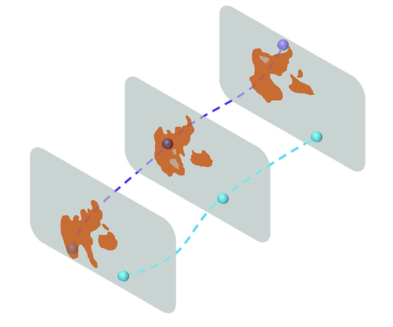
A schematic diagram illustrating the effect of
 $Qs$
structures on the wall-normal transport of particles in turbulent channel flow. (a) Side view of instantaneous
 $Qs$
structures extracted from the flow field. (b) Illustration of a wall-parallel plane. The red patches represent
 $Qs$
structures, and the spheres indicate particles located either inside or outside
 $Qs$
structures. The number of spheres reflects the approximate proportion of particles inside and outside
 $Qs$
structures. Blue arrows indicate wall-normal particle momentum fluxes, with the light blue arrow representing fluxes outside
 $Qs$
structures, and the dark blue arrow representing fluxes inside. The wider dark blue arrow indicates that
 $Qs$
structures, though occupying a small fraction of the total volume (
 $\phi (V)_{Qs} \lt 10\,\%$
), contribute a disproportionately large share of the total particle momentum flux [
 $\phi (\mathcal{F}_M)_{Qs} \approx 20{-}30\,\%$
]. (c) Illustration of particle trajectories relative to
 $Qs$
structures. Red patches denote
 $Qs$
structures, while blue spheres represent particles transported inside
 $Qs$
structures, and red spheres represent particles transported outside. Dashed lines trace the particle trajectories across three instants (
 $t0$
,
 $t1$
and
 $t2$
), with spheres shown at each time step. To better illustrate the wall-normal displacement, the initial position at time
 $t0$
is also marked at time
 $t2$
, and the vertical distance between the two is annotated as
 $\Delta y_p$
, indicating the wall-normal displacement of the particle. This schematic demonstrates that particles inside
 $Qs$
structures tend to travel longer vertical distances, emphasising their key role in enhancing wall-normal transport.

4. Conclusions
The effect of
 $Qs$
structures on the wall-normal transport of particles in turbulent channel flow at
 $Re_\tau = 1000$
has been analysed by data from direct numerical simulations. The particle flux and transport efficiency are quantified in the presence of the
 $Qs$
structures.
A schematic diagram (figure 13) is drawn to illustrate the effects of
 $Qs$
structures on the particle transport. Despite occupying a small volume fraction of the domain,
 $Qs$
structures play a crucial role in the wall-normal transport of both fluid momentum and particles. Both particle number and momentum flux inside the
 $Qs$
structures are larger than those outside them. Additionally, the fraction of wall-normal momentum flux inside
 $Qs$
structures exceeds the volume fraction of
 $Qs$
structures, indicating an enhanced transport efficiency inside the
 $Qs$
structures. The effectiveness of
 $Qs$
structures in transporting inertial particles becomes more pronounced as particle inertia decreases. Furthermore, the continuous effect of
 $Qs$
structures on particles is explored. As shown in figure 13(c), particles are transported to larger wall-normal locations under the continuous influence of the
 $Qs$
structures compared to the particles outside. This implies that the transport of particles, such as sand particles during a storm, could potentially be estimated by identifying
 $Qs$
structures in turbulent flows, as revealed by our findings.
Funding
This work is supported by the Natural Science Foundation of China (grant nos 12388101, 92252104 and 92252204).
Declaration of interests
The authors report no conflict of interest.



