Process

The PERL script ‘AlleleCoder.pl’ is available in Supplemental material S1 (available online at http://journals.cambridge.org). System requirements are a computer with PERL, BioPerl, R, R Commander (including Tcl/Tk) (Stajich et al., Reference Stajich, Block, Boulez, Brenner, Chervitz, Dagdigian, Fuellen, Gilbert, Korf, Lapp, Lehväslaiho, Matsalla, Mungall, Osborne, Pocock, Schattner, Senger, Stein, Stupka, Wilkinson and Birney2002; Fox, Reference Fox2005; R Development Core Team, 2011) installed; a two-button mouse is helpful for interacting with the 3D plot. We used versions 5.10.1 (PERL), 1.6.1 (BioPerl), 2.10.1 (R) and 1.5-4 (R commander).

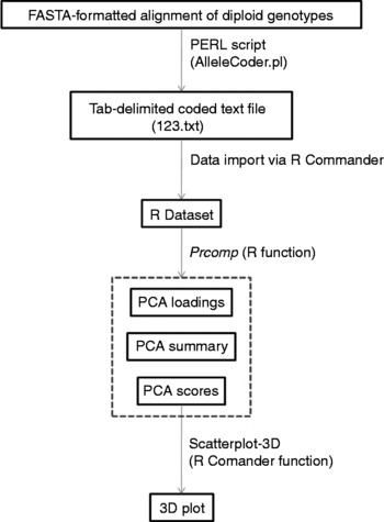
An overview of the process is shown in Fig. 1. Supplemental material S2 (available online at http://journals.cambridge.org) explains software installation and use. For the input file, diploid genotypic data are represented as single unphased aligned nucleotide sequences in FASTA format (Pearson and Lipman, Reference Pearson and Lipman1988). In unphased data, for heterozygotes the diploid genotype is known but constituent haplotypes are unknown. Alleles consist of five possible characters A, C, G, T or – (deletion). Homozygous states of the alleles are indicated in exactly that way. Heterozygous positions are specified by the appropriate IUPAC code (e.g., M R, W, …). Heterozygous deletions are indicated as lowercase a, c, g, t. Characters other than heterozygous indels must be uppercase. A missing data point is coded as N. The PERL script is used to convert aligned nucleotides into a text file containing columns with coded genotype relationships (see Supplemental material S2 for command line format, available online at http://journals.cambridge.org). Genotypes are coded as follows: the homozygous state of the major (more frequent allele in the sample) allele is ‘1’, the homozygous state of any minor (less frequent allele in the sample) allele is ‘3’, the heterozygous state with one major allele is ‘2’, any heterozygous state with no major allele is ‘3’. This results in a heterozygote value (2) numerically intermediate between the two homozgotes (1, 3). Columns identical after they are coded are only represented once in the coded text file. This conserves space and reflects the fact that PCA only considers unique columns.

Fig. 1

Flow diagram of process used to implement and display PCA of genetic diversity. Output files generated by R are enclosed in the hatched box (PCA loadings, PCA summary, PCA scores). ‘PCA scores’ is the file used to display a scatter plot of relationships.

This 123.txt file (Fig. 1) is imported into R using R Commander (see Supplemental material S2 for menu functions, available online at http://journals.cambridge.org). A combination of the commands prncomp and prcomp are then used to perform the PCA. A summary can be generated, which shows what proportion of the variation is explained by each axis. A table with loadings can be generated to show the contribution of each column to each principal component. The PCA scores are generated for each sample, which can then be plotted. Samples can be visualized along PCA axes in two or three dimensions. Scatterplot-3D, a part of the R Commander package, is convenient for 3D visualization.

We have used this method to illustrate genetic diversity and divergence of tomato germplasm accessions held at the USDA-ARS Plant Genetic Resources Unit, Geneva, NY. Cultivated tomato (Solanum lycopersicum L.) dispersed out of Latin America beginning in the 16th century. Worldwide patterns of genetic diversity in tomato are of interest for purposes of conservation, characterization, and utilization. A sample of 50 Plant Genetic Resources Unit (PGRU) accessions (unique populations) was assembled to survey the primary centres of diversity: Chile, Ecuador and Peru (14 accessions), countries contiguous with the primary centres (six accessions), and secondary centres of diversity (30 accessions). The original year of seed collection ranged from 1905 to 2002. Based on SNP alleles of 67 markers (Supplemental material S3, available online at http://journals.cambridge.org) the first three principal components explained 20, 10 and 6.6% of the variation, respectively. Genotypes from primary and secondary centres of diversity were spread along axis PC1, while samples from countries contiguous with the primary centres were distributed along axis PC3 (Supplemental Figure S1, available online at http://journals.cambridge.org). Ten percent of accessions were outliers that fell outside the three ellipsoids encompassing 90% of the variation for each group. These highly diverged genotypes originated from Peru, Ecuador, USA, Europe and Asia. None of the three a priori defined groups should be viewed as a poor source of tomato genetic diversity in PGRU's collection. Results for major outliers (AVRDC #6, Peto 460 and PI 258478) were similar to PCA via a covariance matrix using an independent set of 49 DNA sequences (Labate et al., Reference Labate, Sheffer, Balch and Robertson2011).

Conclusion

AlleleCoder in conjunction with PCA is a useful tool for characterizing diversity among closely related genetic resources, including individuals, populations and species. One advantage of this method is that if a particular axis (i.e. for any of the principal components) separates the data in a biologically meaningful way, those polymorphisms that contribute to that principal component can be identified from the table of PC loadings and used as diagnostic markers. Another advantage of this method is that it accepts unphased polymorphisms, which is helpful when analyzing small sample sizes or data sets comprising species rather than populations.