1. Introduction
The problem of retirement affects all countries, and the issue of which system is ideal has been one of great controversy. Poorly managed pension systems can constitute a significant percentage of a country's economy, and the consequences for having low pensions for the general population are dire. For OECD countries, the pension expenditure averages 7.5% of their GDP (OECD, 2019), and several countries have double-digit figures. Current debates on inequality may lead to increases in these numbers in the near future, as pensions are regarded as a form of social spending. For instance, in the euro area, social spending – on healthcare, education, and social protection – has been increasing since 2001, and social protection currently averages around 20% of the countries' GDPs. Of this figure, expenditures on pensions alone average 12.4% of GDP (i.e., accounting for 62% of expenditures on social protection), which is 50% more than the spending on healthcare, and about 170% more than on education (Rodríguez-Vives and Kezbere, Reference Rodríguez-Vives and Kezbere2019).
Starting in 1981 with Chile, many countries have been shifting their systems toward defined contribution (DC) plans. Reasons include an inverted population pyramid, the complexity of rules associated with defined benefit (DB) plans, and the burden of having to make retirement promises that are difficult to fulfill. Most countries have a hybrid system in which special categories of workers – the military, police, firefighters, and teachers, among other public servants – are under a different scheme than the overall population.
The focus of our work is on DC plans, in which workers invest a fraction of their salary every month, typically on a set of funds offered by the state or by financial entities. During the active phase, also called the accumulation period, it is expected that workers obtain sufficient capital to achieve a reasonable replacement rate, typically around two-thirds of their salary at the time of retirement. Despite the complexity of pension fund schemes, a few key parameters play a fundamental role in the design of the system. The contribution rate, for example, has a major impact on a worker's final pension. Another central aspect of any DC system is how the money is invested in order to reach a certain goal. Life-cycle strategies (Viceira, Reference Viceira and Lusardi2009), which start with investments that have higher risk and return (e.g., equities) and migrate to bonds as retirement approaches, are widely adopted and have an appealing rationale. Most default strategies and target funds available in the market are based on the life-cycle logic.
In the literature, the problem of deciding an appropriate investment strategy for an individual over time is referred to as the glide-path problem. Estrada (Reference Estrada2014) analyzes strategies – called contrarian – opposed to the typical life-cycle strategies, and shows that contrarian strategies can achieve higher expected return, albeit with greater volatility. Mladina (Reference Mladina2016) discusses a time-dynamic asset allocation model with cash-flow goals. Yoon (Reference Yoon2010) proposes a risk-controlled dynamic asset allocation scheme for target funds that explicitly incorporates changes to the term structure of risk. Laster et al. (Reference Laster, Vrdoljak and Suri2016) analyze risks for the glide-path problem after the accumulation phase, sometimes referred to as the ‘glide-through’ problem, as opposed to the classical ‘glide-to’ problem. The authors consider four different risks and discuss mitigation strategies.
We propose an investment model that can be adapted to any DC plan, provided that there are enough data to estimate asset returns and correlations. In this work, we use data from the Chilean pension system, which are publicly available, and already deflated, so the returns reported are real (as opposed to nominal). Moreover, the Chilean DC system is one of the oldest in the world, and it is relatively ‘pure’ in the sense that it is not mixed with a DB component. Mandatory contribution rates will soon be raised to 15% of earnings for all workers, and so we use this value as a fixed number in our models. The value of 15% of income is often cited as an adequate contribution rate (see, e.g., Wasik, Reference Wasik2015; Rupert, Reference Rupert2016).
Throughout the paper, we use the terminology of open-loop and closed-loop policies. An open-loop policy is a decision rule for investing that depends solely on the time until retirement; i.e., it is unaffected by other information that can evolve randomly over time, such as the current wealth. A closed-loop policy can take into account such states of the system; i.e., the actions can depend on the outputs generated by the system or process under consideration including current wealth.
Our main contribution is to study and compare investment strategies in DC plans. To this end, we consider as a benchmark the open-loop policy currently in place in Chile. The Chilean system has five funds A, B, C, D, and E, defined by their exposure to equities, meaning that fund A is riskier but offers higher expected returns, and fund E is less volatile (fixed income products), but has lower expected returns. Mexico, Hungary, and Peru have default strategies in place that are very similar to that in Chile. In Estonia, Lithuania, and Latvia, workers who do not actively decide where to invest their savings are assigned to an analog of fund E. Chilean workers are free to choose in which funds they invest, and can also modify their investments freely. A default policy exists to assign an investment strategy for workers who do not choose in which fund(s) to invest. The default policy in Chile, which we describe in detail below, follows the life-cycle logic and depends only on the time to retirement. Somewhat surprisingly, during a 6-month period that includes the 2008 financial crisis, more than 70% of Chilean workers did not choose an alternative to the default strategy (Berstein et al., Reference Berstein, Fuentes and Torrealba2011). Perhaps consistent with this statistic, 76% of workers do not know how many funds exist, and 57% are unaware of the balance in their personal account.
We seek to answer two fundamental questions. First, ‘How good is the Chilean default policy?’ The default policy currently in place is similar to that of many target funds that are popular elsewhere, and so the question is relevant for virtually all countries and agencies with DC plans. The second question is, ‘Can we find a closed-loop policy that is superior to the default policy?’ Unlike the default policy, in which the strategy is clearly specified, it is not obvious how to formulate a problem that will generate good closed-loop policies.
We follow Basu et al., Reference Basu, Byrne and Drew2011 and use wealth as the state variable, which provides feedback in our time-dynamic asset allocation model. In contrast to Basu et al. (Reference Basu, Byrne and Drew2011), our model considers a broader universe of investment possibilities. Smith (Reference Smith2011) focuses on specific measures of risk in a DC-plan, using expected replacement ratio and pension-at-risk at retirement as metrics at the end of the accumulation period. Our work takes a similar perspective: we ignore the volatility of the journey and believe that what matters is the distribution of wealth at the date of retirement. We consider one base formulation and analyze several different objectives, focusing on utility functions rooted in second-order stochastic dominance (SSD) but also considering traditional utility functions. The former allows us to incorporate the default policy as a benchmark in the model, while the latter allows us to capture risk aversion using the classic framework of von Neumann and Morgenstern (Reference von Neumann and Morgenstern1953). In both approaches, we report out-of-sample performance through metrics such as expected shortfall and probability of reaching a retirement goal.
We cast our models using stochastic dynamic programming (DP), and we discuss how the results shed light on the life-cycle investment logic. Our approach differs from other work that uses stochastic DP (e.g., Viceira, Reference Viceira2001; Michaelides and Gomes, Reference Michaelides and Gomes2005; Horneff et al., Reference Horneff, Maurer and Mitchel2020) in that we focus on risk and on the performance relative to the benchmark, rather than the economic behavior of the worker. Blomvall and Shapiro (Reference Blomvall and Shapiro2006) consider a dynamic portfolio optimization problem with a utility function objective for terminal wealth, but with no additional cash inflows throughout the planning horizon. They show that if there are no transaction costs and the process is stage-wise independent, the optimal policy is myopic (i.e., one can solve a time-static model rather than a time-dynamic multi-stage model) under power and logarithmic utility functions. This result does not apply to a typical pension problem in which workers can simultaneously manage their wealth and make regular cash-inflow contributions from their income.
We disregard the modeling of consumption because our focus is to understand the effectiveness of asset allocation under a fixed contribution rate of 15%. One of our findings is that the default strategy performs surprisingly well, despite being an open-loop policy. However, we show that having in place a system that monitors each worker individually, and changes investment strategies according to the individual's level of wealth, can reduce shortfall relative to a specified retirement target. Finally, our results also show that in the Chilean system, only a small fraction of the investment universe is actually relevant for the design of good investment policies.
2. Closed-loop policies
We introduce a closed-loop policy on a finite (and fixed) planning horizon in which investment decisions depend on the time left until retirement, and on the amount of wealth at each point in time. We obtain a policy that establishes, at each time period (year), an investment allocation as a function of the state variable, which in our case is wealth.
2.1 Problem primitives and notation
We consider an asset allocation problem in which investment decisions are taken at discrete moments in time over a fixed planning horizon, i.e., the accumulation phase. In particular, we consider a planning horizon of T years, and decisions are taken at the beginning of each year. A worker can choose freely among a given set of assets (or funds), and we assume that her additional contributions are made at the end of each year. The amount of the contribution is a fraction, c t, of her annual income, I t, which we assume to be deterministic. Our framework can easily accommodate a stochastic model for salaries, but again for simplicity, we consider deterministic growth and focus instead on the effect of asset allocation. Moreover, in line with most DC systems, the fraction c t is constant throughout the accumulation phase. We assume workers to be risk averse when it comes to their pension, and so the goal for each worker is to accumulate as much wealth as possible, while accounting for the risk of the investment strategy, which will be made precise later. A pure maximization of expected return is undesirable as the resulting return distribution would have high volatility, and therefore significant downside risk.
The model's state variable, X t ∈ ℝ+, tracks the wealth at the beginning of time period t. For a given set, ${\cal F}$ , comprised of $n = \vert {\cal F} \vert$
 funds, the action space is defined as all convex combinations of investments in the funds. We simplify the action space by considering allocations that involve at most two funds and in discrete allocation amounts. In particular, for a set Λ = {0, 0.05, …, 0.95, 1.0} of discrete allocations, the set of actions that we consider is defined by ${\cal A} = \lcub {a\in {\rm {\opf R}}_ + ^n\ \colon\ a_i = \lambda \comma \;a_j = 1-\lambda \comma \;a_k = 0\quad \forall i\comma \;j\comma \;k\in {\cal F}\comma \;\forall \lambda \in \Lambda \comma \;i\ne j\ne k} \rcub$
 . For example, in a system with three funds, i.e., n = 3 and ${\cal F} = \lcub {f_1\comma \;f_2\comma \;f_3} \rcub$
 , the action $\lsqb {0.3\comma \;0.0\comma \;0.7} \rsqb \in {\cal A}$
 implies that 30% of the current wealth is invested in fund f 1 and 70% is invested in fund f 3. Let ξ t be an n-dimensional random vector that models the returns for each asset at time period t. Returns are realized after making the allocation decision in period t, but the joint probability distribution of the returns is assumed to be known for all time periods $t\in {\cal T}$
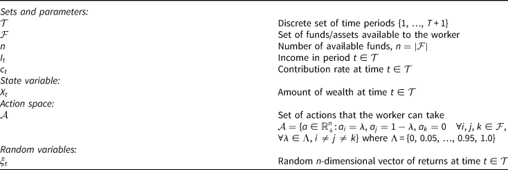
 at the beginning of the planning horizon. Wealth from time period t to t + 1 grows according to these realized returns plus the contribution during period t, which is assumed to be received at the end of that period. Table 1 summarizes the model's notation, including the parameters described in the problem statement.
Notation of the stochastic dynamic program

2.2 Stochastic dynamic programming model
As is standard in DP, we formulate the model via a recursion that represents the value function V t(X t) for a given level of wealth X t:

where

Equation (1) defines V t(X t) as the maximum across all possible actions in ${\cal A}$ of an objective function that considers the value of future stages. There is no immediate reward as the wealth only has a meaningful value at the end of the planning horizon. Hence, the objective at stage t is to maximize the expected value of future rewards by taking an action $a_t\in {\cal A}$
 . Action a t and random returns ξ t define the return of the portfolio for stage t, and ${\rm {\opf E}}_{\xi _t}\lsqb{\cdot} \rsqb$
 denotes the expectation operator with respect to ξ t, although we typically suppress this dependence. Equation (2) defines the transition of the state variable, which takes into account the returns from invested wealth and the additional contribution, c tI t. At stage T + 1, no further actions are taken, and the final wealth is evaluated via the performance measure ρ(X T+1; ⋅), which maps the random variable X T+1 to a real number. The “dot” notation in ρ's argument allows us to distinguish different choices for ρ as will become clear below. Hence, equation (1) for t = T is defined as:

with X T+1 defined as in (2). The choice of ρ(X T+1; ⋅) is crucial in our goal of providing a policy that accumulates as much wealth as possible while accounting for risk. In particular, ρ(X T+1; ⋅) serves as the mechanism to optimize as it provides a notion of ordering between different wealth distributions at time T + 1 that would be obtained under different sequences of actions.
Solving this DP formulation yields an investment policy along the planning horizon that varies according to the accumulation of wealth. It is worth emphasizing that this is a computationally tractable DP model because of the univariate state and modest size of the action space. The univariate state variable allows us to have a fine discretization of the state space, which yields a high-fidelity policy as a function of wealth. The action space grows with the number of funds and allowable discrete allocations, but even with a moderate number of funds, the investment possibilities at every time period will be large given the number of elements in Λ.
In principle, one could increase the number of funds, but in practice, it could be overwhelming for some workers to choose among too many options. In 401(k) plans in the United States, despite the vast universe of investment options, target date funds (TDFs) dominate the market (Avallone, Reference Avallone2018). TDFs can be easily constructed in our framework by choosing one fund to represent the stocks, another to represent bonds and change the allocation as time evolves to reflect a smaller exposure to assets. Moreover, as we discuss in Section 3, having more funds may not be necessary, at least when we consider those available in the current Chilean system. Furthermore, the expectations in the model are also tractable as we can have a discrete representation of the joint probability distribution of the returns, and we assume inter-period independence of the return vector.
We provide a brief description of how the stochastic dynamic program in (1) is solved via backward recursion. As we indicate above, the action space ${\cal A}$ comprises a discrete set of portfolios available to the worker. We estimate expectations in (1) via sample means from N independent and identically distributed (i.i.d.) realizations of the returns generated as described in Section 3.2. Finally, the state variable X t is discretized on a grid ${\cal S}$
 = {0, Δ, 2Δ, …, x max} with resolution Δ, which allows us to obtain a high-fidelity representation of the value function V t(X t). Algorithm 1 shows pseudo-code of the backward induction procedure. In step 6, the floor operator $\lfloor \; \cdot \; \rfloor$
 indicates that the value is rounded down to the closest value in ${\cal S}$
 so the function V t+1( ⋅ ) is computed at these prespecified values. Appendix A provides further implementation details.
Algorithm 1: Backward induction
Require : ρ, performance function; ξ 1, …, ξ N, annual i.i.d. realizations of the returns; ${\cal S}$ , state space discretization; ${\cal A}$
 , action space discretization.
Ensure : U, lookup table for the policy.
1: Set $V_t\lpar x \rpar \leftarrow 0\quad \forall x\in {\cal S}\comma \;t\in {\cal T}$

2: Set $U_t\lpar x \rpar \leftarrow null\quad \forall x\in {\cal S}\comma \;t\in {\cal T}$
3: Set $V_{T + 1}\lpar x \rpar \leftarrow \rho \lpar {x\semicolon \;\cdot } \rpar \quad \forall x\in {\cal S}$
4: for t = T, T − 1, …, 1 do
5: for x ∈ ${\cal S}$
do
6: $a^\ast{\in} \mathop {arg\;max}\limits_{a_t\in {\cal A}} {1 \over N}\sum _{\omega = 1}^N V_{t + 1}\lpar \lfloor{{\lpar {\xi^\omega } \rpar }^{\rm \top }a_tx + c_tI_t} \rfloor\rpar$
7: $U_t\lpar x \rpar \leftarrow {a^\ast\ {\triangleright}}$
Save optimal action8: $V_t\lpar x \rpar \leftarrow {1 \over N}\sum _{\omega = 1}^N V_{t + 1}\lpar \lfloor{{\lpar {\xi^\omega } \rpar }^{\rm \top }a_tx + c_tI_t} \rfloor\rpar$
9: return U


In what follows, we discuss a broad class of models by defining the performance measure ρ(X T+1; ⋅) using SSD and traditional utility functions. The goal in most of the models we discuss is to obtain a policy that is, in some sense, superior to a benchmark. The benchmarks that we employ involve: (i) a mix of the stochastic wealth distribution derived from a default policy, which is typically available in a pension system, and (ii) a deterministic target goal, e.g., 66% replacement rate. We emphasize that throughout the development of alternatives for ρ(X T+1; ⋅), the core form of the model remains unchanged as specified by recursion (1)–(2) for $t\in {\cal T}$ and terminal condition (3).
2.3 Ranking alternatives
Methods for ranking alternatives whose outcomes are stochastic have a long history in economics and finance. Given two alternatives with random outcomes, a decision maker is interested in ranking these alternatives in order to select the one that she prefers. For example, the study of lotteries in economics arises both in theory and in practical experiments, and has contributed to a better understanding of decision making under uncertainty. Lotteries are also a fundamental tool for behavioral economics, and were an important element in the development of prospect theory (Kahneman and Tversky, Reference Kahneman, Tversky, MacLean and Ziemba2013). When instead of comparing a few alternatives we want to optimize over a large, and potentially infinite, set of alternatives, the problem is more involved because every feasible alternative typically has a different distribution of outcomes. Here, we start with the aspiration of designing a closed-loop policy that any risk-averse decision maker would prefer over a benchmark policy. The benchmark we consider is derived from a default policy (typically imposed by the government) that is the de facto choice for people who do not choose their investment strategy.
To cope with this aspiration, we investigate two approaches that tackle the preference conundrum from different viewpoints and embed them in the stochastic dynamic program described above. First, we review the theory of stochastic dominance and describe several models that impose preference over the default policy directly. We then use more traditional utility functions to model risk aversion independently of which default policy is in place.
2.3.1 Second-order stochastic dominance
Given a benchmark, stochastic dominance provides a way to impose a preference among alternatives with stochastic outcomes. The concept of stochastic dominance compares two random variables via a performance metric. First-order stochastic dominance (FSD) compares real-valued random variables using the cumulative distribution function (CDF). A random variable X dominates a random variable Y in the first order if

with F X(η) = ℙ(X ≤ η). Following a similar idea, SSD uses the following performance metric for a random variable X:

A random variable X dominates a random variable Y in the second order if

which is denoted by $X{\rm \succeq }_{SSD}Y$ .
We focus on SSD because of its close connection with risk aversion. While FSD guarantees that the expected value of any non-decreasing utility function evaluated at X and Y favors X over Y, SSD ensures the same but for any non-decreasing concave utility function (i.e., risk-averse utility functions). Since there is a natural justification for being risk averse in the context of pensions, we used SSD instead of the more demanding FSD concept. For a discrete random variable Y with finite support ${\cal Y} = \lcub {y_1\comma \;y_2\comma \;\ldots \comma \;y_{n_Y}} \rcub$ , inequality (6) can be re-written in terms of expected shortfall with a finite number of constraints as described by Dentecheva and Ruszczyński (Reference Dentecheva and Ruszczyński2006), [Proposition 1]. Hence, we can replace inequality (6) with:

where ( ⋅ )+ = max{ ⋅ , 0}. We use the SSD inequality (7) to motivate the development of certain forms for ρ(X T+1; ⋅).
We assume the default policy has a probability distribution governing terminal wealth that we can characterize via simulation. We further assume that we can similarly characterize the probability distribution governing the terminal wealth associated with using the policy derived from the dynamic program. The goal is to come up with a closed-loop policy with a terminal wealth distribution that dominates that of the default policy. To this end, let X T+1 be the random variable that represents the terminal wealth using a DP-based policy, and let Y T+1 be the random variable representing the terminal wealth under the default policy. Our preference could then be imposed via the following constraint:

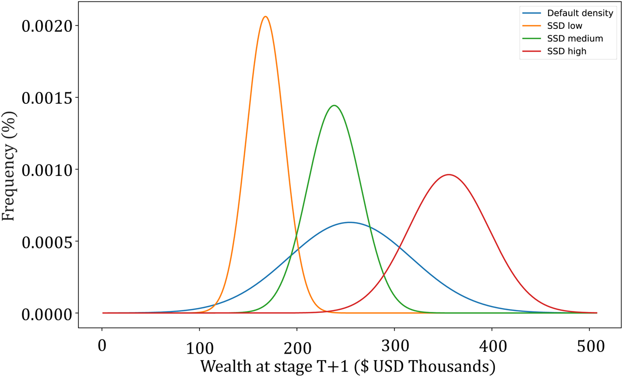
Through the lens of optimization, inequality (8) is a requirement rather than an aspiration, and this has two important implications. First, we would like to maximize the ‘distance’ by which X T+1 dominates Y T+1 because inequality (8) may be viewed as a ‘minimum’ requirement. Second, in the sense of inequality (7), our preference for domination may differ based on different points $y\in {\cal Y}$ . Before defining performance measures, ρ(X T+1; ⋅), motivated by (8), we note that X T+1 as defined in this section is only available via simulation upon solving the dynamic program. In the DP model at stage T, the wealth X T at the beginning of the time period is given, and therefore the terminal wealth is conditioned to this value. Hence, in the same way that expectations in (1) for 1 ≤ t ≤ T − 1 are computed in a conditional manner in the DP, we will work with the conditional random variable X T+1|X T rather than the unconditional X T+1. Figure 1 shows the type of random variables being compared, with the distribution of wealth using the default policy depicted in blue. Conditioned on having a low, medium, or high level of wealth at the beginning of stage T, we can depict the distribution of the final wealth under a particular action a T. In this sense, the goal is to seek a family of SSD requirements between the distribution of wealth obtained with the default policy (which is unconditional and denoted by Y T+1) and the distribution of wealth in the DP, X T+1|X T, i.e., the wealth conditioned on X T.
Representation of terminal wealth under the SSD policy conditioned on having low, medium, and high accumulated wealth at the beginning of stage T + 1.

We employ a performance measure, ρ(X T+1;Y T+1, β), parameterized by Y T+1 and a real-valued parameter, β. Let

be the slack variable in inequality (7) for support point $y\in {\cal Y}$ , so that satisfying constraint (7) corresponds to s(X T+1, Y T+1, y) ≥ 0 for all $y\in {\cal Y}$
 . The first specific model we consider is based on the following:

where ${\cal Y}_\beta = \lcub {y\in {\cal Y} \,\colon \, y \le \beta } \rcub$ is the support of Y T+1 truncated at β. Plugging equation (10) as the value function at T into equation (3) fully specifies the DP model, and seeks a notion of domination of X T+1 over that obtained under the default policy, Y T+1, by seeking to maximize an equally weighted sum of the slack variables, at least for $y\in {\cal Y}_\beta$
 . We focus on $y\in {\cal Y}_\beta$
 because of risk aversion. For example, if we select β to be the deterministic goal, say G, then we focus on dominating the default policy when it performs poorly relative to the goal rather than focusing on more aggressive outcomes that exceed the goal. Note that the terms in (10) that involve Y T+1 simply form an additive constant, and the expected shortfalls that are computed for X T+1 are with respect to the subset of support points given by ${\cal Y}_\beta$
 . In this sense, we may view equation (10) as a piecewise linear concave utility function in which the kink points are motivated by the default policy.
A natural alternative to (10) is to consider the smallest slack across the n Y inequalities, as opposed to the sum. This modification of the performance measure, which also accounts for ${\cal Y}_\beta$ , is as follows:

If the DP-based policy does not dominate the default policy at every $y\in {\cal Y}_\beta$ , i.e., negative values of s(X T+1, Y T+1, y) arise, then the DP model based on equation (11) minimizes the expected value of the worst-case violation. In our numerical results in Section 3, we consider performance measures defined by both (10) and (11), and experiment with different values of the parameter β.
2.3.2 Traditional utility functions
Another approach to risk aversion uses ‘traditional’ utility functions, which are pervasive in economics due to their ability to rank alternatives with respect to a decision maker's preferences. In the context of pension funds, utility functions help to model risk preferences of a worker. To incorporate a utility function, u( ⋅ ), for terminal wealth, we define:

The problem of maximizing terminal wealth with a utility function has been extensively studied in the literature, especially in continuous time (Merton, Reference Merton1969; Merton, Reference Merton1975). In discrete time, we have the seminal work of Samuelson (Reference Samuelson1975), which considers a lifetime portfolio selection problem. However, the framework differs from our work in two aspects: there is consumption at every time period, and there are no portfolio constraints. More recent work (Bick et al., Reference Bick, Kraft and Munk2013) considers a consumption-investment problem that incorporates portfolio constraints. To deal with those constraints, the authors develop a new methodology called SAMS, which is based on ideas from artificial markets developed in Cvitanic and Karatzas (Reference Cvitanic and Karatzas1992). The algorithm has no convergence proof, and the parameter calibration step is highly problem-dependent. So, in what follows, we use stochastic DP for the traditional utility functions as well.
Like the SSD-based approach, our expectation with respect to X T+1 is conditioned on X T. While this performance measure does not explicitly reference the benchmark Y T+1, we can incorporate the target wealth G in defining our utility functions:


Equation (13) defines a power function that is a risk-averse utility for values for γ > 0 (γ ≠ 1). This utility belongs to the class of constant relative risk aversion functions, and risk aversion increases with γ. Here, the parameter G provides a normalizing constant to help interpret results, but an optimal policy for one G holds for all G > 0 for utility (13). Equation (14) defines a sigmoidal utility function that, for appropriate values of the κ-parameters (e.g., κ i > 0, i = 1, 2, 3), characterizes a risk-seeking investor for small values of wealth who becomes increasingly risk-averse as the wealth approaches and then exceeds the target level G. Under utility (14), the optimal policy is sensitive to the specified goal G.
Both utility functions (13) and (14) are only used in the last time period as a mechanism to evaluate terminal wealth. While this parallels our SSD-motivated utility functions, it stands in contrast to other models in which utility functions are used at every time period to trade units of utility among different time periods, e.g., by increasing consumption before retirement. While both utility functions may be suitable for the DC pension fund problem, fitting the parameters to a particular person's preferences is a difficult task (e.g., Schechter, Reference Schechter2007; Rabin, Reference Rabin2013). Nonetheless, it is worth studying how different utility functions shape the investment policy and its performance.
3. Numerical results
In this section, we compare the policies obtained with each of the DP formulations described above, i.e., under SSD-motivated utilities and under traditional utility functions. Our experiments are based on the Chilean system, which we describe next.
3.1 Case study
The Chilean pension system is managed by private asset managers, called AFP by their Spanish acronym, who are regulated by the government and whose sole activity by law is to manage the workers' savings. The system is set up in such a way that there are five different funds (labeled A, B, C, D, E) in which a worker can choose to invest her money. These funds are supposed to have long-term average returns in decreasing order, meaning that fund A has the highest return and fund E is the most conservative fund. The experimental setup is as follows:
• the accumulation phase is assumed to be T = 40 years;
• there are five funds available, ${\cal F} = \lcub {A\comma \;B\comma \;C\comma \;D\comma \;E} \rcub$
;• the initial yearly salary is I 1 =10,000 and it grows 2% per year during the accumulation phase so that the final salary is IT = 21,634;
• the fraction of income that is contributed is fixed to c t = 0.15 for all time periods; and
• the target value, G, is the net present value of 18 years (life expectancy upon retirement) of 66% of the final income (I T), which is often regarded as an appropriate annual replacement rate. With the input parameters for income and risk-free discount factor δ, $G = 0.66\sum _{t = 1}^{18} I_T\delta ^t = \$ 220\comma 683$
.


As mentioned above, there is evidence that around 70% of the working population in Chile do not actively manage their retirement funds, and the government allocates the savings of such workers to a fund depending solely on the worker's age and gender. We refer to this strategy as the default policy. The policy for men (women) starts with a full allocation in fund B until the person is 35 years old. After the age of 35, the strategy transfers 20% of the allocation per year to fund C so that at the age of 40, the full allocation is in fund C. The investment remains in fund C until the person is 55 (50) years old, and in the next year, it starts to transition to fund D in 20% steps. By the age of 60 (55), the allocation is fully in fund D until the end of the accumulation phase. This strategy is an open-loop policy in the sense that it does not depend on the state, i.e., the wealth accumulated at any point in time.
3.2 Return data and random variate generation
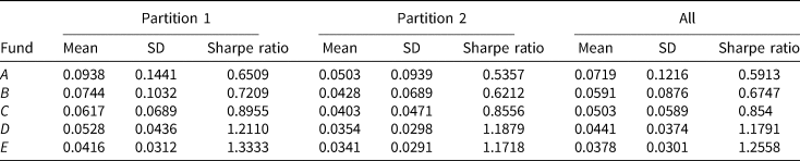
Data for the Chilean system, which can be downloaded from https://www.spensiones.cl/apps/valoresCuotaFondo/vcfAFP.php, encompasses 191 months of returns from the year 2002 – when the five funds were created – until 2018. Table 2 summarizes the mean, standard deviation, and Sharpe ratio (computed with a risk-free rate of zero) of the annualized returns for each fund.
Mean, standard deviation and Sharpe ratio of annualized return data

In our DP formulations, expectations are with respect to the joint distribution of the five-dimensional vector for fund returns. To fit a probabilistic model to data and to be able to generate observations from this distribution, we used the NORTA procedure (Cario and Nelson, Reference Cario and Nelson1996; Cario and Nelson, Reference Cario and Nelson1997). NORTA stands for normal-to-anything, and is a copula-based approach to fit a multivariate random vector with arbitrary marginal distributions. The procedure's inputs are: (i) the marginal distribution for each fund's return, and (ii) the covariance matrix of the five-dimensional random vector. Using $\left({{5}\over{2}}\right)$ bivariate normal copulas, NORTA matches exactly the specified marginals, and seeks pairwise correlation coefficients for the bivariate copulas to match the covariance matrix given as input. This matching procedure uses a separate binary search for each correlation coefficient. Upon fitting these parameters, we obtain a mechanism to generate as many i.i.d. random vectors as desired from the fit distribution. NORTA's principal advantage is that it allows for general marginal distributions and captures first-order dependence between the random returns. We use the empirical distribution of the data as the marginal distributions, and the empirical covariance matrix to provide requisite inputs (i) and (ii). We use the entire data set (i.e., 191 monthly returns) to fit NORTA, as our goal is to construct a policy for the entire accumulation phase ‘today’, but using ‘past’ information. Note that despite using normal copulas to obtain the desired correlation, there is no normality assumption on the distributions of the returns. For our DP models, the NORTA simulation procedure allows us to estimate all expectations using sample means, and we can increase the sample size until the resulting policies exhibit little change. In our case study, temporal correlation of the returns was negligible and therefore disregarded; however, in the presence of temporal correlation, a sequel version of NORTA, VARTA (Biller and Nelson, Reference Biller and Nelson2003), can be used instead.
Since the time resolution in the DP formulation is years and we fit monthly returns, we obtain a stream of 12 five-dimensional vectors from NORTA to form a single yearly return. To compute the expectations in our DP formulations, we use Monte Carlo sampling with 1,000 i.i.d. return vectors, and we use this same set of realizations for all time periods, i.e., the joint probability distribution is assumed to be stationary and we assume temporal independence. The default policy is also simulated to obtain a distribution of its terminal wealth that is later used in the SSD-based formulation. Since no optimization is involved, we approximate Y T+1's distribution using 10,000 i.i.d. replications under the default policy. For the SSD-based policies, we define ${\cal Y}_\beta$ with 100 support points by truncating ${\cal Y}$
 at β first, and then selecting 100 points corresponding to percentiles of the truncated distribution.
Aside from the expectations used to compute the DP policies, we draw additional realizations of the returns to perform an out-of-sample simulation of the policies. To do so, we generate 10,000 independent realizations of the returns to simulate the wealth process under each policy, again assuming that the worker starts with no savings and an initial income of I 0 = 10,000. We use common random numbers so that all policies use the same set of 10,000 i.i.d. returns in the out-of-sample testing.
3.3 Out-of-sample performance
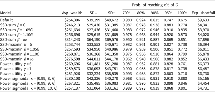
We conduct an out-of-sample test in which the performance of a policy is simulated to assess the distribution of terminal wealth if a worker were to adopt that policy. Table 3 summarizes the results of 14 policies derived from the solution of a DP model, i.e., the DP models associated with utilities (10), (11), (13), and (14), and a selection of parameters, i.e., β for SSD-based models, γ for the power utility, and (κ 1, κ 2, κ 3) for the sigmoidal utility. Our selection of the parameters for each model is as follows: β ∈ {G, 1.05G, 1.10G, ∞}, γ ∈ {6, 7, 8}, κ 1 = 0.99, κ 2 ∈ {8, 9, 10}, and κ 3 = 6. Other values of the parameters are admissible, and our particular selection solely attempts to illustrate our methodology for a prototypical user for which those parameters capture her risk aversion. For the power utility function, we tested values of γ ∈ (1, 10], which are considered acceptable (see, e.g., Mehra and Prescott, Reference Mehra and Prescott1988; Ang, Reference Ang2014), and we report results for cases in which the mean return was roughly comparable with that of the default policy. Different utility functions would be admissible under this framework, provided that the necessary parameters are available. In Table 3, column 1 specifies the model and the corresponding parameters; column 2 shows the mean of the final wealth; columns 3–4 show the standard deviation decomposed into the negative and positive semideviations; columns 5–9 show the probability of reaching a particular fraction of the target wealth; and finally, column 10 shows the expected shortfall, relative to the target, i.e., ${\mathbb E}$ [(G − X T+1)+]. We include the results of the default policy in the first row. Our implementation of NORTA can be downloaded at https://github.com/dukduque/NortaPy, or directly installed in Python via pip install norta.
Out-of-sample performance results for different DP-based policies and the default policy

A worker who needs to choose among these policies has a broad spectrum of choices in terms of risk and return considerations. The default policy provides the benchmark performance metrics. The foremost advantage of any of these policies with respect to the default policy is a reduction in downside risk. Expected shortfall is significantly less for all the policies, ranging from 18% to 59% reduction in this metric. For each of the four sets of models, there is at least one selection of the parameters in Table 3 for which not only is there an improvement in downside risk, but a larger average wealth is also attained. Taking a closer look at the behavior of each policy at lower percentiles of terminal wealth, it is worth noting how the probability of reaching a terminal wealth as low as 70% of the target tends to be close to 0.98 (the default policy's value), while for 80%, 90%, 95%, and 100% of G, the DP-based polices tend to outperform the default, sometimes by substantial margin. If we consider the negative semideviation for each policy (SD−), relative to its average wealth, the DP-based policies perform consistently better than the default in the following sense: for ‘SSD-sum’ with β = ∞, for example, the average wealth value minus the SD− value is $250,053, compared with $215,107 for the default policy.
Regardless of which policy is selected by a worker, there are two main insights from these results. First, the default policy performs relatively well for being an open-loop policy, i.e., a policy that does not have the option of adapting as a function of the cumulative wealth. This policy exceeds the target wealth on average, and the probability of accumulating <70% of G is <0.02. Nevertheless, there is room for significant improvement by using closed-loop policies that offer a similar – and more often than not, larger – average wealth and substantially less downside risk. Specifically, our closed-loop policies offer better chances of achieving 70%, 80%, 90%, and 100% of the target wealth; for example, the policy obtained with the SSD-sum model (β = 1.10G) increases the probability of reaching 100% of the target from 0.675 to 0.870 and reduces the expected shortfall by almost 60%.
So far, our analysis of the performance of the DP policies has been aggregated. We now study one policy from each of the four DP families and reference them by the name of the model only, i.e., we drop the parameter values that specify the model. In particular, we analyze the policies associated with: SSD-sum (β = 1.10G), SSD-maxmin (β = 1.05G), power utility (γ = 7), and sigmoidal utility (κ = (0.99, 9, 6)).
3.4 DP-based policies
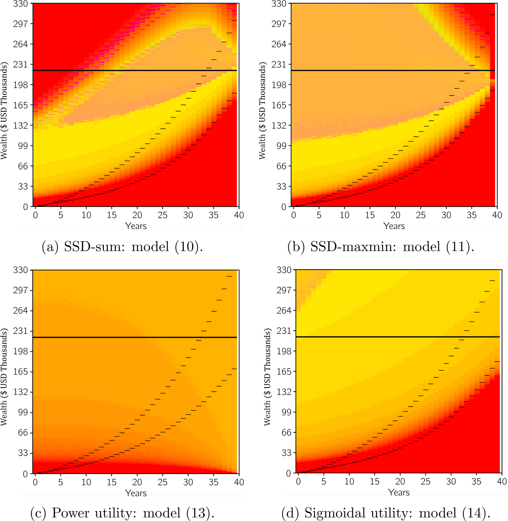
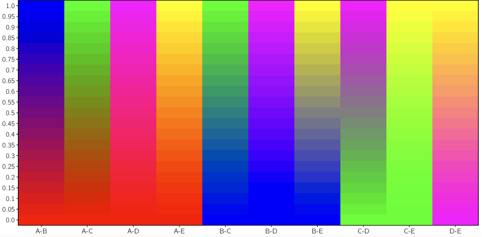
We depict DP-based policies in a two-dimension plane in which the x axis denotes time, the y axis denotes wealth, and a color map encodes the action to take in each time-period and wealth-level pair. Our action space, ${\cal A}$ , contains 195 (19 × 10 + 5) actions that correspond to all possible pair-wise combinations of funds in discrete steps of 0.05. Appendix A discusses empirical sensitivity, or lack thereof, to selecting a finer grid. To build a color map to represent actions, a full investment in A, B, C, D, or E is encoded in red, blue, green, magenta, and yellow, respectively; see Figure 2. Combinations of these colors, e.g., red and yellow, represent a portfolio with two funds. In what follows, all the policies, except for the default, use primarily funds A and E (red and yellow), and we make precise the exact action that corresponds to different colors when describing the policies. Appendix B describes the color encoding for portfolios combining two funds.
Action color map for all five funds.

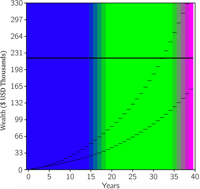
Figure 3 depicts the default policy described in Section 3.1. The main colors encoding actions in this policy are blue, green, and magenta, which represent full allocations in funds B, C, and D, respectively. Also, since it is an open-loop policy, the action implied by the policy is independent of wealth. Transitions from B to C and from C to D happen in steps of 20%. The solid black line marks the target value G and the dashes denote the 5th and 95th percentiles for each year of the wealth distribution simulated in the out-of-sample test.
Default policy representation and 5th and 95th percentiles of the out-of-sample policy simulation for all time periods.

Figure 4 depicts the policy obtained with each variation of the four DP models. The format of the figures is the same as that of Figure 3. The foremost distinction between these policies and the default policy is the fact that the action to be taken varies according to time and level of wealth. Moreover, the funds that are used by these policies are mainly funds A and E, which is in contrast with the default policy, which uses funds B, C, and D. We also note that all four polices follow a life-cycle strategy for most of the accumulation phase. An interesting feature of the SSD-based policies is that they become aggressive again if the cumulative wealth is high relative to the distribution of wealth associated to the default policy. This is a feature that the models using traditional utility functions do not possess due to the risk-averse structure of these functions at high levels of wealth. At early stages of the accumulation phase, all policies start with a full allocation in fund A. The transition to allocations that combine funds A and E varies for each policy, but in general this occurs more quickly when the portfolio experiences good performance. The allocation in late stages grows to 30–70% for funds A–E for the power utility model and 15–85% for the sigmoidal utility model. In the SSD-based models, the obtained policy uses mostly funds A and E, and few times use combinations of D and E in late stages of the accumulation phase.
Policies obtained with DP formulations for SSD and both traditional utility models.

In light of Blomvall and Shapiro (Reference Blomvall and Shapiro2006), and also Merton (Reference Merton1969), we now reconsider the power utility function from Figure 4(c), except that we replace the 15% annual contribution of income with a 0% contribution. Solving the resulting model with our DP procedure yields a solution of 25% allocation to asset A and 75% to asset E, and that allocation is independent of time and wealth. This is consistent with the results of Blomvall and Shapiro (Reference Blomvall and Shapiro2006), as discussed in Section 1, and corresponds to a special case in which the DP can be replaced by solving a myopic one-period asset allocation model because we have temporal independence of returns, no transaction costs, and no annual contribution. Under a non-zero (e.g., 15%) annual contribution, the myopic approach would only serve as a heuristic, and the DP approach is required to obtain an optimal policy.
3.5 Policy assessment
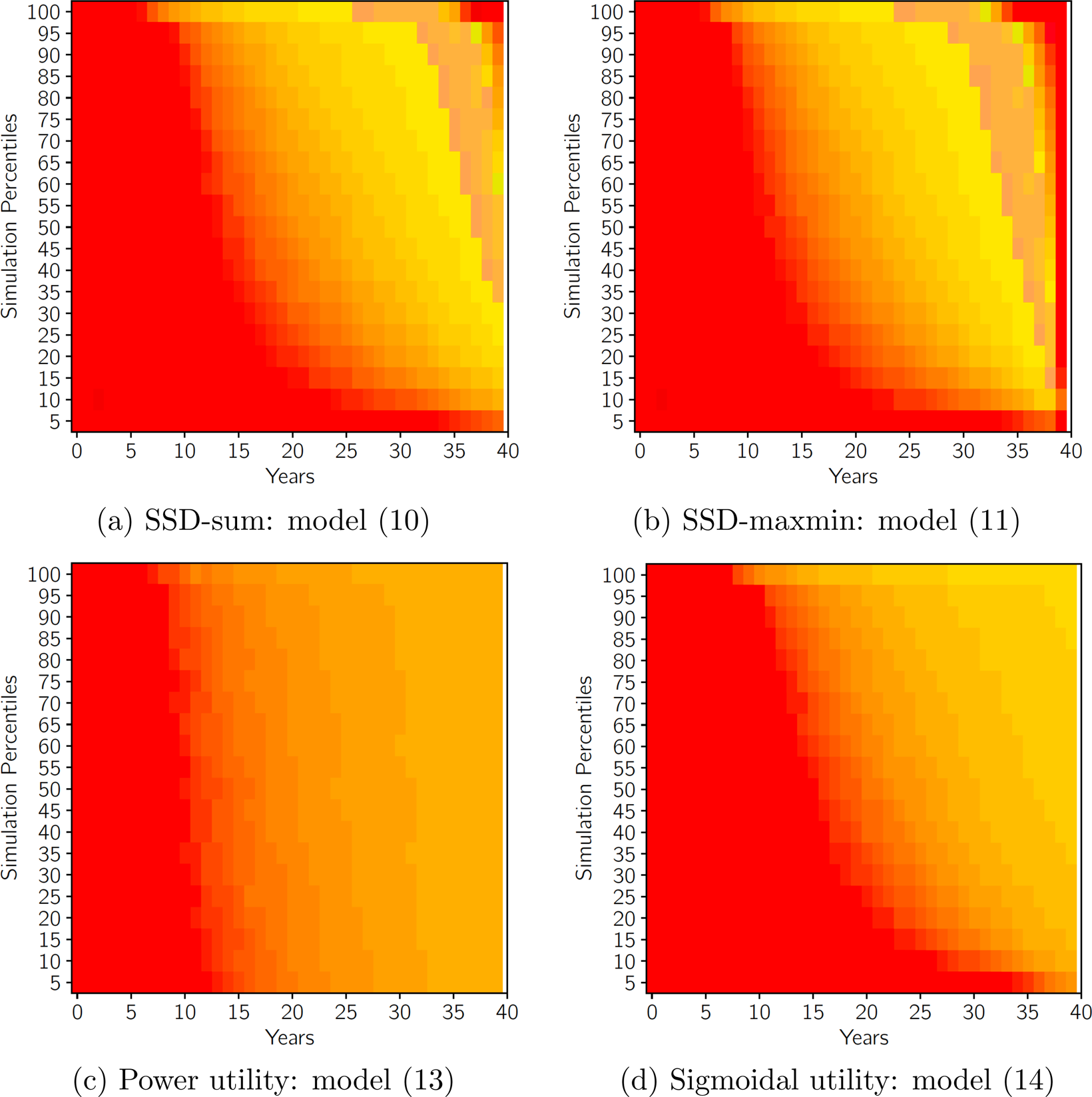
Figure 5 plots the same four policies shown in Figure 4, but assumes that wealth throughout the years is a particular percentile of its out-of-sample simulation. For example, at the 5th and 95th percentiles in Figure 5, we observe the policy that a worker should use if her wealth were to evolve according to the dashed lines in Figure 4. Similarly, at the 50th percentile, we observe the policy that a worker should follow if wealth is at its median value throughout the years. Although this constant behavior in the returns is unrealistic, these plots allow us to characterize the policies in terms of the performance observed during the accumulation phase. In all cases, the transition from fund A to fund E starts earlier when the wealth is growing faster (i.e., high percentiles) and the transition is delayed when the funds are under performing (i.e., low percentiles). Except for the last 5–10 years in the accumulation phase, the policies have somewhat similar qualitative behavior.
Policies described in terms of wealth percentiles obtained with DP formulations for both the SSD models and the traditional utility models.

For the 50th percentile, the policy for the SSD-sum model starts with fund A and remains there for 12 years. After this, the policy transitions, in steps of 5–10% to combinations of funds A and E. In year 20, the policy allocates 45% of the wealth in fund A and 55% of the wealth in E. At this point, it is worth comparing the action suggested by the DP with that of the default policy. The 45–55% combination of funds A and E has an expected annual return of 4.98% with a standard deviation of 6.02%. In the same year, the default policy suggests fund C, which has an average annual return of 4.74% with a standard deviation of 6.13%. Such examples are pervasive as funds B, C, and D can – given the data on returns – effectively be replicated (or improved) by combinations of funds A and E. Following the 50th percentile example, by year 30, the portfolio positions are 20% in fund A and 80% in fund E, and the accumulation phase ends with a 25–75% position in funds D and E. This terminal-year portfolio is another example in which the DP policy obtains a portfolio that dominates the one suggested by the open-loop policy (i.e., a full position in fund D) in terms of mean and standard deviation. Similar behavior is seen for the policy obtained with the SSD-maxmin model and the sigmoidal utility model, albeit with some differences in the last few years of the accumulation phase. The policy obtained with the power utility model is considerably different. The differences between the percentiles are less pronounced. Looking at the 50th percentile again, the transition to fund E starts in year 8. In year 20, the position of the portfolio in A and E is 45–55%, by year 30 is 35–65%, and by year 32 is 30–70% until the end of the horizon.
3.6 Comparison with the default policy
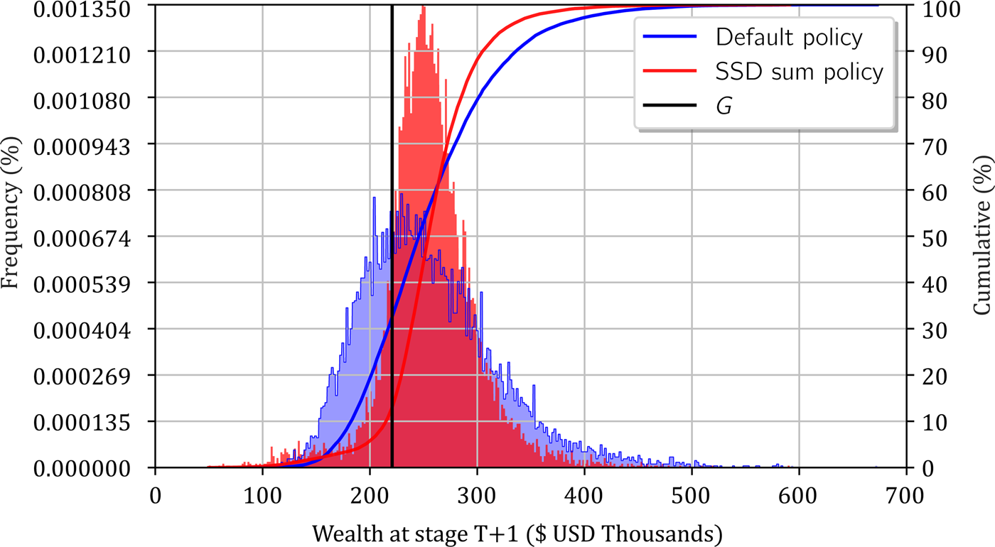
This section presents a head-to-head comparison between the policy from the SSD-sum model (again with β = 1.10G) and the default policy. Figure 6 shows the terminal wealth distribution for the default policy, and the SSD-sum model in blue and red, respectively. The left y-axis indicates the relative frequency of the distribution and the right y-axis indicates the CDF. The vertical black line marks the target wealth G. As expected from the model, and as also shown in Table 3, the distribution of the SSD-sum policy is shifted to the right, dominating the default policy until well above the goal G.
Comparison of the terminal wealth densities and distributions (curves) in dollars under the default- and SSD-sum policies.

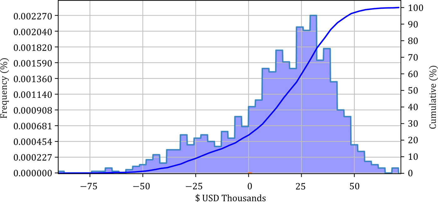
To better understand the lower tails of the distributions, we further analyze the subset of sample paths – out of the 10,000 simulations in the out-of-sample tests – in which both policies achieve a terminal wealth below the target value G. For these 1,275 samples, we analyze the difference in terminal wealth of both policies. In other words, we look at the performance of the policies when both underperform, due to poor returns, in order to obtain insight regarding the downside risk of the policies.
Figure 7 depicts the distribution of the difference in wealth obtained by these two policies, conditioned on underperforming. Positive values mean that the SSD-sum policy performed better. As one would expect from a risk-averse policy, when returns are low, and losses relative to the goal occur, the risk-averse policy performs better on average. For these sample paths, the default policy is on average $14,700 below the SSD-sum policy, which delivered superior returns in 78% of the cases. The remaining 22% are cases of low-performing sample paths (e.g., multiple losses throughout the accumulation phase) that account for <3% of the 10,000 total sample paths.
Density and distribution of terminal wealth (in dollars) under the SSD-sum policy minus that of the default policy, restricted to sample paths in which both fall short of the goal G.

3.7 Robustness of the policies
So far in our analysis, we have used the same distribution of the returns to compute DP-based policies as well as to simulate them, i.e., the samples used to compute expectations and to generate sample paths in the simulations come from the same random stream (distribution) given by the NORTA procedure. In order to assess the robustness of the policies that we present above, we now turn to a cross-validation analysis in which the distribution of the returns used to compute the policy (i.e., to solve the dynamic program) differs from the distribution used in the simulation. To this end, we partition the data in two sets to distinguish between training and testing data. The training data are used to compute (train) the policy, and the testing data are used to simulate the policy's performance. Let S 1 and S 2 partition the data such that $S_1\cup S_2$ is all data and $S_1\cap S_2$
 is empty. Of 191 available months, S 1 comprises the first 95 months of the data while S 2 comprises the remaining months. For each set in the partition, we carry out the NORTA procedure to obtain two streams of random vectors to model the returns of the funds. Table 4 shows the mean, standard deviation, and Sharpe ratio of the annualized returns for each fund and time-slice, including the full data as a reference from Table 2.
Mean, standard deviation and Sharpe ratio of annualized returns for both time slices and for the full set of data

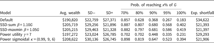
Table 5 shows the out-of-sample performance, repeating the metrics from Table 3, for the default policy and a subset of the DP-based policies. Here, the DP-based policies are trained using data from the first partition (i.e., S 1). However, the simulation is conducted using data from the second partition (i.e., S 2). Despite having strikingly different results compared to Table 3, e.g., the probability of reaching 100% of G, the tendency of obtaining DP-based policies, which better control downside risk, remains. In particular, the model based on SSD-sum manages to get both a better average wealth, and a smaller expected shortfall compared to the default policy. Similarly, the policy based on the power utility function gets better average wealth and expected shortfall, despite having a smaller probability of reaching 70% of the target wealth than that of the default policy. Differences between these results and those of Table 3 are expected because the distribution of the returns used in the simulations is substantially different in each case; again, see Table 4.
Out-of-sample performance: training the policy on S 1 and testing performance on S 2

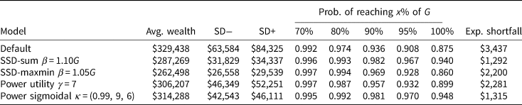
Finally, we switch the roles of S 1 and S 2. Table 6 shows performance metrics from simulating using the first set of the partition (i.e., S 1), when the DP-based policies are trained using data from the second set of the partition. As before, our goal is to assess out-of-sample performance when the distribution of the returns (test) differs from the distribution used to compute the policy (train). In this experiment, once again the downside risk of DP-based policies is better than that of the default policy, although in contrast to the results of Tables 3 and 5, the average wealth is lower, e.g., 12% lower for SSD-sum. It is worth reiterating that here we chose a particular parametrization of the policy (e.g., β = 1.10G for SSD-sum or γ = 7) ahead of time, and then performed the simulation. In practice, we could replicate this cross-validation exercise for various values of the parameters to assess the trade-off between average wealth and expected shortfall.
Out-of-sample performance: training the policy on S 2 and testing performance on S 1

4. Conclusions
In this work, we propose closed-loop policies for asset allocation in DC pension systems, which depend on the worker's cumulative wealth at each year in the accumulation phase. To build these policies, we formulate a stochastic DP model that uses different objective functions to take risk aversion, the performance of the default policy, and a target terminal wealth into account. The objective functions are motivated by SSD relative to the performance of a default policy, as well as more traditional utility functions.
We tested the performance of the closed-loop policies using data from the Chilean system. The system comprises five funds, and monthly data from the past 16 years were used to calibrate the stochastic returns of the model. We first used SSD to propose a policy that is superior to the default policy used by the government for workers who do not choose their investment strategy. The default policy in Chile is an open-loop policy in which investment decisions are only based on the age and gender of the worker, and that policy only uses three out of the five available funds. Additionally, we parameterized some of our utility functions to reward beating a pre-defined target corresponding to a replacement rate of 66% of a worker's terminal salary. All the models discussed obtained a significant reduction in downside risk, and almost all resulted in expected returns that were superior to those of the default policy. Additionally, the probabilities of reaching a fixed percentage of the final target was almost always significantly superior when closed-loop polices are employed. Lastly, we observed multiple cases in which the allocations used in the closed-loop policies dominated returns from the allocations in the default policy. In particular, by combining the riskier and less risky funds in the system, our models were able to obtain allocations with better expected return and lower volatility than the ones used by default policy.
In summary, our work advocates replacing default policies by closed-loop alternatives that take into account the wealth of the worker at a given time. Further research is necessary to determine whether defined contributed systems offering many types of funds have advantages. In our results for the Chilean system, two out of five funds were not used at all in our policies and a third fund was seldom used. Another interesting question to address in future work is whether the interest rate at retirement, which affects the annuity received by retirees, has an impact on the designed policy and if so, how can it be included in our model. In the current scenario of negative interest rates, this topic will increase in relevance, and probably different mechanism designs will have to be proposed to improve post-retirement plans. Finally, we plan to investigate whether deciding the timing of retirement can have a significant impact on terminal wealth.
Acknowledgements
The authors would like to thank Patrick and Amy McCarter for their support through the 2018-2109 Patrick and Amy McCarter Fellow in Residence. This research was supported, in part, by Northwestern University’s Center for Optimization & Statistical Learning and by FONDECYT grant 1170178.
Appendix A. Implementation details
In our computations, we set x max = $3 × 10⁶ and Δ = $50. Our choice of x max is sufficiently large relative to the terminal wealth that can be attained for the given income profile, contribution rate, and average returns. In practice, this value can be estimated via a simple calculation of the wealth process under the riskiest fund, and a given contribution profile. On the other hand, our choice of Δ is small enough so that we do not observe differences in the out-of-sample performance with smaller values of this parameter.
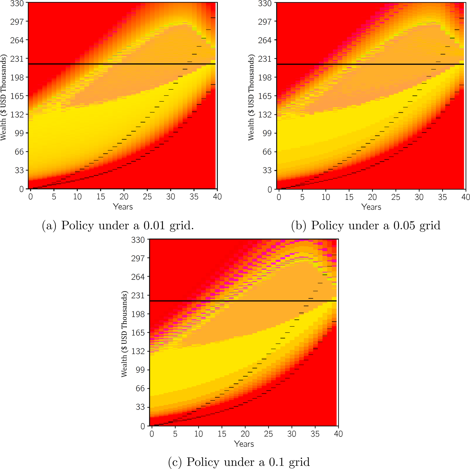
We discretize the action space on a grid of 0.05 as described in Section 2.1. A finer grid would provide a higher-fidelity policy at the expense of greater computational effort. We opted for the 0.05 level of resolution because changes in the final policy and its performance appear negligible for finer grids. Figure A.8 shows the policies obtained using the same DP-based model but under different grid sizes, namely, a grid of 0.01 in Figure A.8(a), a grid of 0.05 in Figure A.8(b), and a grid of 0.1 in Figure A.8(c). We also compute the performance metrics that we studied throughout the paper, and compare them in Table A.7. The differences that we observe are rather negligible, and the computational effort on a personal laptop is 3.45 min for the 0.1 grid, 8 min for the 0.05 grid, and 53 min for the finer 0.01 grid.
Policies under three resolutions of the grid for the action space for the SSD-sum model (β = 1.1G).

Out-of-sample performance results for different grid sizes for the action space for the SSD-sum model (β = 1.1G)

Appendix B. Action map color encoding
Figure B.9 shows the color encoding for actions that represent portfolios with two funds, and it serves as the legend for the figures showing different DP-based policies throughout the paper. For a particular pair of funds (e.g., A–B) and a given allocation value (e.g., 0.3), the corresponding color encodes the action of investing this fraction in the second fund (0.3 in B) and the rest in the first fund of the pair (0.7 in A). Allocation values of 0.0 or 1.0 denote a full investment in either the first or the second fund for each pair of funds, e.g., an allocation value of 0.0 in the A–B pair encodes with red a full allocation in fund A.
Action color map for all possible investments on combinations of the five funds.