1 Introduction
Near-inertial waves (NIWs) are generated in the ocean mixed layer by wind-stress forcing with the 1000 km horizontal scale characteristic of ocean storms (Pollard Reference Pollard1980; D’Asaro et al. Reference D’Asaro, Eriksen, Levine, Paulson, Niiler and Meurs1995). But as a result of interaction with the mesoscale and submesoscale eddy field, NIWs quickly develop smaller horizontal length scales (Klein & Treguier Reference Klein and Treguier1995; Lee & Niiler Reference Lee and Niiler1998; Klein & Llewellyn Smith Reference Klein and Llewellyn Smith2001; Klein, Llewellyn Smith & Lapeyre Reference Klein, Llewellyn Smith and Lapeyre2004; Zhai, Greatbatch & Zhao Reference Zhai, Greatbatch and Zhao2005; Danioux, Klein & Rivière Reference Danioux, Klein and Rivière2008). This reduction in length scale is crucial in explaining the relatively rapid vertical propagation of NIWs into the thermocline: if NIWs retain the 1000 km scale characteristic of windy generation, then there is no vertical propagation on sensible time scales (Gill Reference Gill1984). Thus the interaction of NIWs with macroturbulence is crucial to the characterization of upper-ocean physical variability.
Young & Ben Jelloul (Reference Young and Ben Jelloul1997) used a multiple time scale approach to derive a phase-averaged equation, hereafter the YBJ equation, describing the slow evolution of NIWs in a quasi-geostrophic eddy field. The YBJ equation captures three key processes that shape the near-inertial spectral peak: (i) wave dispersion; (ii) advection of NIWs by geostrophic velocity; (iii) refraction and focussing of NIWs by geostrophic vorticity.
The important dimensionless parameter in the asymptotic development of the YBJ equation is the Burger number
 $$\begin{eqnarray}\mathit{Bu}\stackrel{\mathit{def}}{=}\left(\frac{Nk}{fm}\right)^{2},\end{eqnarray}$$
where
 $k$
and
 $m$
are horizontal and vertical wavenumbers of the NIW and
 $N$
and
 $f$
are the buoyancy and Coriolis frequencies. A characteristic feature of the YBJ expansion – justified by
 $\mathit{Bu}\ll 1$
– is that the pressure gradient does not appear at leading order. Thus the leading-order horizontal velocity of NIWs can be represented compactly as
 $$\begin{eqnarray}u+\text{i}v=\text{e}^{-\text{i}ft}\mathsf{L}\,A,\end{eqnarray}$$
where
 $\mathsf{L}$
is the frequently occurring differential operator
 $$\begin{eqnarray}\mathsf{L}\stackrel{\mathit{def}}{=}\unicode[STIX]{x2202}_{z}\frac{f^{2}}{N^{2}}\unicode[STIX]{x2202}_{z},\end{eqnarray}$$
and
 $A(x,y,z,t)$
is a complex field;
 $\mathsf{L}\,A$
is the ‘backrotated velocity’. Other leading-order NIW quantities, such as the vertical velocity and the pressure, can be expressed in terms of
 $A$
as in (2.10) through (2.12) below.
The propagation of NIWs through a geostrophic flow has recently been examined by (Thomas, Smith & Bühler Reference Thomas, Smith and Bühler2017, TSB hereafter). With numerical solutions of the Boussinesq equations, TSB show that the modulation of NIWs by a geostrophically balanced flow depends crucially on the relative size of two small parameters:
 $\mathit{Bu}$
in (1.1) and the Rossby number
 $\mathit{Ro}$
of the geostrophic flow. The YBJ equation is a reductive approximation based on the distinguished limit in which
 $\mathit{Bu}\rightarrow 0$
with the ratio
 $\mathit{Ro}/\mathit{Bu}$
fixed. In other words, while
 $\mathit{Bu}$
and
 $\mathit{Ro}$
can be varied independently in the parent Boussinesq equations, only the ratio
 $\mathit{Ro}/\mathit{Bu}$
appears the YBJ equation: the size of the parameter space has been reduced. This is a useful prediction of the YBJ equation: for sufficiently small
 $\mathit{Bu}$
, only the ratio
 $\mathit{Ro}/\mathit{Bu}$
is decisive in determining the modulation of NIWs by geostrophic flow.
In realistic situations, however, there is a spectrum of geostrophic eddies and also a spectrum of NIWs, and there is neither a unique
 $\mathit{Ro}$
nor a unique
 $\mathit{Bu}$
characterizing the flow. In other words, for some component NIWs of the near-inertial spectral peak
 $\mathit{Ro}/\mathit{Bu}$
is large, while for other components
 $\mathit{Ro}/\mathit{Bu}$
is small: NIWs will be modulated to varying degrees by macroturbulence resulting in complex spatial patterns. To capture these diverse regimes, TSB recommend separating the solution into vertical modes and employing different phase-averaged equations based on the ratio
 $\mathit{Ro}/\mathit{Bu}$
associated with the gravest horizontal scale. A limitation of this approach is that even NIWs sharing a single vertical mode number might – depending on the horizontal scale
 $k^{-1}$
– have very different values of the ratio
 $\mathit{Ro}/\mathit{Bu}$
.
Motivated by these results of TSB, and also by numerical difficulties encountered in the solving the YBJ equation (see below), here we propose an improved version of the YBJ equation. This YBJ+ equation is
 $$\begin{eqnarray}\unicode[STIX]{x2202}_{t}\mathsf{L}^{\!+}A+J(\unicode[STIX]{x1D6F9},\mathsf{L}^{\!+}A)+\frac{\text{i}}{2}\triangle \unicode[STIX]{x1D6F9}\mathsf{L}^{\!+}A+\frac{\text{i}f}{2}\triangle A=0,\end{eqnarray}$$
where
 $\triangle \stackrel{\mathit{def}}{=}\unicode[STIX]{x2202}_{x}^{2}+\unicode[STIX]{x2202}_{y}^{2}$
is the horizontal Laplacian and
 $$\begin{eqnarray}\mathsf{L}^{\!+}\stackrel{\mathit{def}}{=}\mathsf{L}+{\textstyle \frac{1}{4}}\triangle .\end{eqnarray}$$
In (1.4),
 $\unicode[STIX]{x1D6F9}$
is the streamfunction of the quasi-geostrophic eddy field and
 $\triangle \unicode[STIX]{x1D6F9}$
is the relative vorticity. We show that YBJ+ has an improved representation of NIW dispersion and is a simpler alternative to the scheme proposed by TSB.
The plain and simple YBJ equation is recovered with the replacement
 $\mathsf{L}^{\!+}\mapsto \mathsf{L}$
in (1.4). In terms of the scaling used to derive (1.4) from the Boussinesq equations, the extra term
 ${\textstyle \frac{1}{4}}\triangle$
in the operator
 $\mathsf{L}^{\!+}$
is order
 $\mathit{Bu}$
smaller than
 $\mathsf{L}$
. Thus YBJ+ is retaining a small term,
 ${\textstyle \frac{1}{4}}\triangle A$
, that is asymptotically negligible relative to the dominant term
 $\mathsf{L}\,A$
. Because of this extra term, YBJ+ depends separately on
 $\mathit{Bu}$
and
 $\mathit{Ro}$
, not just the ratio
 $\mathit{Ro}/\mathit{Bu}$
.
In limiting cases YBJ+ is more accurate than YBJ; moreover YBJ+ has more forgiving numerical properties. Both advantages can be appreciated by considering freely propagating near-inertial waves, i.e.
 $\unicode[STIX]{x1D6F9}=0$
. The YBJ+ dispersion relation is then obtained by substituting
 $$\begin{eqnarray}A=\text{e}^{\text{i}(kx+mz-\unicode[STIX]{x1D70E}^{+}t)}\end{eqnarray}$$
into (1.4). With uniform
 $N$
, one finds that
 $$\begin{eqnarray}\unicode[STIX]{x1D70E}^{+}=\frac{4\mathit{Bu}}{4+\mathit{Bu}}\frac{f}{2},\end{eqnarray}$$
where
 $\mathit{Bu}$
is defined in (1.1). The corresponding YBJ dispersion relation is
 $$\begin{eqnarray}\unicode[STIX]{x1D70E}=\mathit{Bu}\frac{f}{2}.\end{eqnarray}$$
The formal requirement for accuracy of both YBJ and YBJ+ is that
 $\mathit{Bu}\ll 1$
. YBJ is accurate only to first order in
 $\mathit{Bu}$
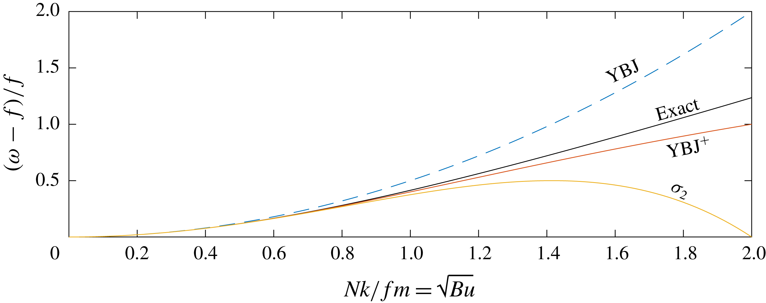
; we show below, and in figure 1, that the YBJ+ dispersion relation is accurate to order
 $\mathit{Bu}^{2}$
. This enhanced accuracy addresses the issues raised by TSB and is certainly welcome. But in our view enhanced accuracy is not the only advantage of YBJ+.
Numerical expediency is also an important advantage of YBJ+ over YBJ: in the YBJ dispersion relation (1.8),
 $\unicode[STIX]{x1D70E}\propto k^{2}$
as
 $k\rightarrow \infty$
. To resolve these waves explicitly one needs to decrease the time step proportionally with the number of horizontal grid points. This is impractical even with modest horizontal resolution. On the other hand, because
 $$\begin{eqnarray}\lim _{\mathit{Bu}\rightarrow \infty }\unicode[STIX]{x1D70E}^{+}=2f,\end{eqnarray}$$
the YBJ+ model has no such high-wavenumber restriction on the size of the time step. The YBJ+ time step must be short enough to ensure stable integration of oscillations with frequency
 $2f$
; this requirement is independent of horizontal resolution. Explicit schemes can thus be used to integrate YBJ+.


One can, of course, avoid numerical instability by using an unconditionally stable, implicit time-stepping scheme. But implicit schemes distort the high-wavenumber structure of the dispersion relation. In particular, one can show that integration of the YBJ equation with the Crank–Nicolson scheme results in a numerical dispersion relation that is qualitatively similar to
 $\unicode[STIX]{x1D70E}^{+}$
in (1.7): as
 $k\rightarrow \infty$
the ‘Crank–Nicolson
 $\unicode[STIX]{x1D70E}$
’ asymptotes to a constant frequency as in (1.9). We prefer to guarantee numerical stability by a physically motivated modification of the model equation, rather than by relying on implicit time stepping. And there are compelling reasons to believe that for waves with
 $\mathit{Bu}$
of order unity, YBJ+ is significantly more accurate than YBJ.
The enhanced accuracy of YBJ+ over YBJ can be appreciated by comparing the dispersion relations in (1.7) and (1.8) with the exact dispersion relation for hydrostatic internal waves
 $$\begin{eqnarray}\unicode[STIX]{x1D714}=f\sqrt{1+\mathit{ Bu}}.\end{eqnarray}$$
With
 $\mathit{Bu}\ll 1$
, the dispersion relations in (1.7) and (1.10) produce the Taylor expansion
 $$\begin{eqnarray}\unicode[STIX]{x1D714}-f=\left[\mathit{Bu}-\frac{1}{4}\mathit{Bu}^{2}+\text{ord}(\mathit{Bu}^{3})\right]\frac{f}{2}.\end{eqnarray}$$
Thus
 $\unicode[STIX]{x1D70E}^{+}$
agrees more closely with the exact dispersion relation (1.10) than does the YBJ
 $\unicode[STIX]{x1D70E}$
in (1.8): see figure 1. In fact, (1.7) is a simple Padé sum of the two-term Taylor series in (1.11) and boasts the robust numerical properties of these approximations. For example, with
 $\mathit{Bu}=3$
, the exact frequency from (1.10) is
 $\unicode[STIX]{x1D714}=2f$
, while
 $f+\unicode[STIX]{x1D70E}^{+}=13f/7$
. In other words, with the small parameter equal to 3, the error in the YBJ+ dispersion relation (1.7) is 7 %.
TSB proposed another improved description of NIW propagation. Their ‘intermediate dispersion regime’ model is
 $$\begin{eqnarray}\unicode[STIX]{x2202}_{t}\mathsf{L}\,A+J(\unicode[STIX]{x1D6F9},\mathsf{L}\,A)+\frac{\text{i}}{2}\triangle \unicode[STIX]{x1D6F9}\mathsf{L}\,A+\frac{\text{i}}{2}\,f\triangle A-\frac{\text{i}}{8}\triangle ^{2}\mathsf{L}^{-1}A=0,\end{eqnarray}$$
where
 $\mathsf{L}^{-1}$
is the inverse of the operator
 $\mathsf{L}$
in (1.3). This model has the dispersion relation
 $$\begin{eqnarray}\unicode[STIX]{x1D70E}_{2}=\left[\mathit{Bu}-\frac{1}{4}\mathit{Bu}^{2}\right]\frac{f}{2},\end{eqnarray}$$
which, like YBJ+, is in second-order agreement with the expansion of the exact dispersion relation (1.10). But
 $\unicode[STIX]{x1D70E}_{2}\propto k^{4}$
as
 $k\rightarrow \infty$
, and the stability condition on time stepping (1.12) is therefore even more restrictive than that of YBJ. Moreover, although
 $\unicode[STIX]{x1D70E}^{+}$
and
 $\unicode[STIX]{x1D70E}_{2}$
have the same formal level of accuracy,
 $\unicode[STIX]{x1D70E}^{+}$
is more accurate if
 $\mathit{Bu}$
is of order unity: see figure 1. TSB show that in integrations over long times, YBJ develops significant phase errors with respect to the exact shallow-water equations; the model in (1.12) is significantly more accurate than YBJ in this respect. On the basis of figure 1, we anticipate that YBJ+ will at least match, and probably exceed, the long-time phase accuracy of (1.12).
To show how the Padé-summed dispersion relation (1.7) arises, in § 2 we derive the YBJ+ equation in the simple case
 $\unicode[STIX]{x1D6F9}=0$
. In § 3 we discuss the conservation laws (action and coupled energy) of YBJ+. In § 4 we compare solutions of YBJ and YBJ+ with solutions of the Boussinesq equation; this comparison confirms that YBJ+ is more accurate than YBJ. Conclusions are presented in § 5.
2 Derivation of YBJ+
In this section we derive (1.4) in the special case
 $\unicode[STIX]{x1D6F9}=0$
. This minimizes algebraic details and shows clearly how the term
 ${\textstyle \frac{1}{4}}\triangle A_{t}$
arises. We then use physical and heuristic arguments to obtain the higher-order terms with
 $\unicode[STIX]{x1D6F9}\neq 0$
.
2.1 Formulation
The expansion is based on a distinguished limit in which the Burger number, denoted in this section by
 $\unicode[STIX]{x1D716}^{2}$
, is small. Following Young & Ben Jelloul (Reference Young and Ben Jelloul1997) one uses the complex representation
 $$\begin{eqnarray}{\mathcal{U}}\stackrel{\mathit{def}}{=}u+\text{i}v,\quad \text{and}\quad s\stackrel{\mathit{def}}{=}x+\text{i}y.\end{eqnarray}$$
It follows that
 $$\begin{eqnarray}\unicode[STIX]{x2202}_{s}={\textstyle \frac{1}{2}}(\unicode[STIX]{x2202}_{x}-\text{i}\unicode[STIX]{x2202}_{y}),\quad \unicode[STIX]{x2202}_{s^{\ast }}={\textstyle \frac{1}{2}}(\unicode[STIX]{x2202}_{x}+\text{i}\unicode[STIX]{x2202}_{y}),\end{eqnarray}$$
and the horizontal Laplacian is
 $$\begin{eqnarray}\triangle =\unicode[STIX]{x2202}_{x}^{2}+\unicode[STIX]{x2202}_{y}^{2}=4\unicode[STIX]{x2202}_{s}\unicode[STIX]{x2202}_{s^{\ast }}.\end{eqnarray}$$
Other useful results are
 $u_{x}+v_{y}={\mathcal{U}}_{s}+{\mathcal{U}}_{s^{\ast }}^{\ast }$
and
 $v_{x}-u_{y}=\text{i}{\mathcal{U}}_{s^{\ast }}^{\ast }-\text{i}{\mathcal{U}}_{s}$
.
We employ with a multiple time scale expansion
 $$\begin{eqnarray}\unicode[STIX]{x2202}_{t}=\unicode[STIX]{x2202}_{t_{0}}+\unicode[STIX]{x1D716}^{2}\unicode[STIX]{x2202}_{t_{2}}+\unicode[STIX]{x1D716}^{4}\unicode[STIX]{x2202}_{t_{4}}+\cdots\end{eqnarray}$$
Then, with the complex notation outlined in (2.1) through (2.3), the scaled horizontal momentum equation is
 $$\begin{eqnarray}(\unicode[STIX]{x2202}_{t_{0}}+\text{i}f){\mathcal{U}}=-\unicode[STIX]{x1D716}^{2}\unicode[STIX]{x2202}_{t_{2}}{\mathcal{U}}-\unicode[STIX]{x1D716}^{4}\unicode[STIX]{x2202}_{t_{4}}{\mathcal{U}}-\unicode[STIX]{x1D716}^{2}2p_{s^{\ast }}+\text{ord}(\unicode[STIX]{x1D716}^{6}).\end{eqnarray}$$
The other equations of motion are
 $$\begin{eqnarray}\displaystyle & {\mathcal{U}}_{s}+{\mathcal{U}}_{s^{\ast }}^{\ast }+w_{z}=0, & \displaystyle\end{eqnarray}$$
 $$\begin{eqnarray}\displaystyle & \unicode[STIX]{x2202}_{t_{0}}b+wN^{2}=-\unicode[STIX]{x1D716}^{2}\unicode[STIX]{x2202}_{t_{2}}b+\text{ord}(\unicode[STIX]{x1D716}^{4}), & \displaystyle\end{eqnarray}$$
 $$\begin{eqnarray}\displaystyle & p_{z}-b=0. & \displaystyle\end{eqnarray}$$
All fields are expanded in powers of
 $\unicode[STIX]{x1D716}^{2}$
:
 ${\mathcal{U}}={\mathcal{U}}_{0}+\unicode[STIX]{x1D716}^{2}{\mathcal{U}}_{2}+\unicode[STIX]{x1D716}^{4}{\mathcal{U}}_{4}+\cdots$
and so on.
2.2 The expansion
At leading order,
 $\unicode[STIX]{x1D716}^{0}$
, the pressure is negligible in (2.5) and the general solution is
 $$\begin{eqnarray}{\mathcal{U}}_{0}=\mathsf{L}\,A\text{e}^{-\text{i}ft_{0}},\end{eqnarray}$$
where
 $\mathsf{L}$
is the operator in (1.3). Using
 $\mathsf{L}\,A$
in (2.9) facilitates expression of the other leading-order fields in terms of
 $A$
 $$\begin{eqnarray}\displaystyle & \displaystyle w_{0}=-\frac{f^{2}}{N^{2}}A_{zs}\text{e}^{-\text{i}ft_{0}}+\text{cc}, & \displaystyle\end{eqnarray}$$
 $$\begin{eqnarray}\displaystyle & b_{0}=\text{i}fA_{zs}\text{e}^{-\text{i}ft_{0}}+\text{cc}, & \displaystyle\end{eqnarray}$$
 $$\begin{eqnarray}\displaystyle & p_{0}=\text{i}fA_{s}\text{e}^{-\text{i}ft_{0}}+\text{cc}, & \displaystyle\end{eqnarray}$$
where
 $\text{cc}$
denotes complex conjugate.
At order
 $\unicode[STIX]{x1D716}^{2}$
, the horizontal momentum equation is
 $$\begin{eqnarray}(\unicode[STIX]{x2202}_{t_{0}}+\text{i}f){\mathcal{U}}_{2}=-\unicode[STIX]{x2202}_{t_{2}}\mathsf{L}\,A\text{e}^{-\text{i}ft_{0}}-2\text{i}fA_{ss^{\ast }}\text{e}^{-\text{i}ft_{0}}+2\text{i}fA_{s^{\ast }s^{\ast }}^{\ast }\text{e}^{+\text{i}ft_{0}}.\end{eqnarray}$$
Removing the resonant terms gives the leading-order evolution equation
 $$\begin{eqnarray}\unicode[STIX]{x2202}_{t_{2}}\mathsf{L}\,A+2\text{i}fA_{ss^{\ast }}=0.\end{eqnarray}$$
Solving the remnants of (2.13) one obtains
 $$\begin{eqnarray}{\mathcal{U}}_{2}=A_{s^{\ast }s^{\ast }}^{\ast }\text{e}^{+\text{i}ft_{0}}.\end{eqnarray}$$
The ‘reconstituted’ velocity,
 ${\mathcal{U}}_{0}+\unicode[STIX]{x1D716}^{2}{\mathcal{U}}_{2}$
, has the slightly elliptic hodograph characteristic of NIWs.
The second-order vertical velocity follows from (2.6)
 $$\begin{eqnarray}w_{2z}=-A_{sss^{\ast }}\text{e}^{-\text{i}ft_{0}}+\text{cc}.\end{eqnarray}$$
Now we use the leading-order evolution equation in (2.14) to rewrite (2.16) as
 $$\begin{eqnarray}2\text{i}fw_{2z}=\unicode[STIX]{x2202}_{t_{2}}\mathsf{L}\,A_{s}\text{e}^{-\text{i}ft_{0}}+\text{cc}.\end{eqnarray}$$
This reduces the number of
 $x$
and
 $y$
derivatives from three in (2.16) to one in (2.17). Thus YBJ+ avoids the high-order differential operator,
 $\triangle ^{2}$
, in (1.12). Another advantage of (2.17) is that one can now integrate with respect to
 $z$
to obtain the second-order vertical velocity
 $$\begin{eqnarray}2\text{i}fw_{2}=\frac{f^{2}}{N^{2}}\unicode[STIX]{x2202}_{t_{2}}A_{zs}\text{e}^{-\text{i}ft_{0}}+\text{cc}.\end{eqnarray}$$
One rejoices that the boundary condition
 $A_{z}=0$
ensures that both
 $w_{0}$
and
 $w_{2}$
vanish. This integration in
 $z$
avoids the inverse operator
 $\mathsf{L}^{-1}$
that complicates (1.12). For all these reasons, the transition from (2.16) to (2.17) is a crucial technical step in the derivation of YBJ+.
With
 $w_{2}$
in hand, the other second-order fields follow
 $$\begin{eqnarray}b_{2}={\textstyle \frac{1}{2}}\unicode[STIX]{x2202}_{t_{2}}A_{zs}\text{e}^{-\text{i}ft_{0}}+\text{cc},\quad \text{and}\quad p_{2}={\textstyle \frac{1}{2}}\unicode[STIX]{x2202}_{t_{2}}A_{s}\text{e}^{-\text{i}ft_{0}}+\text{cc}.\end{eqnarray}$$
At fourth order, the horizontal momentum equation is
 $$\begin{eqnarray}\displaystyle (\unicode[STIX]{x2202}_{t_{0}}+\text{i}f){\mathcal{U}}_{4} & = & \displaystyle -\unicode[STIX]{x2202}_{t_{4}}{\mathcal{U}}_{0}-\unicode[STIX]{x2202}_{t_{2}}{\mathcal{U}}_{2}-2p_{2s^{\ast }},\end{eqnarray}$$
 $$\begin{eqnarray}\displaystyle & = & \displaystyle -\unicode[STIX]{x2202}_{t_{4}}\mathsf{L}\,A\text{e}^{-\text{i}ft_{0}}-\unicode[STIX]{x2202}_{t_{2}}A_{s^{\ast }s^{\ast }}^{\ast }\text{e}^{+\text{i}ft_{0}}-\unicode[STIX]{x2202}_{t_{2}}A_{ss^{\ast }}\text{e}^{-\text{i}ft_{0}}-\unicode[STIX]{x2202}_{t_{2}}A_{s^{\ast }s^{\ast }}^{\ast }\text{e}^{+\text{i}ft_{0}}.\end{eqnarray}$$
To remove the resonant terms from (2.21), we require
 $$\begin{eqnarray}\unicode[STIX]{x2202}_{t_{4}}\mathsf{L}\,A+\unicode[STIX]{x2202}_{t_{2}}A_{ss^{\ast }}=0.\end{eqnarray}$$
2.3 Reconstitution and remodelling
Following the philosophy of Roberts (Reference Roberts1985), we now ‘reconstitute’ the perturbation series by forming the linear combination (2.14)
 $+$
 $\unicode[STIX]{x1D716}^{2}$
(2.22):
 $$\begin{eqnarray}(\unicode[STIX]{x2202}_{t_{2}}+\unicode[STIX]{x1D716}^{2}\unicode[STIX]{x2202}_{t_{4}})\mathsf{L}\,A+\unicode[STIX]{x1D716}^{2}\unicode[STIX]{x2202}_{t_{2}}A_{ss^{\ast }}+2\text{i}fA_{ss^{\ast }}=\text{ord}(\unicode[STIX]{x1D716}^{4}).\end{eqnarray}$$
On the right-hand side above we indicate that there are higher-order terms that have not been calculated explicitly. One such term is
 $\unicode[STIX]{x1D716}^{4}\unicode[STIX]{x2202}_{t_{4}}A_{ss^{\ast }}$
, which can be rescued from the garbage on the right and moved to the left-hand side of (2.23) so that
 $$\begin{eqnarray}(\unicode[STIX]{x2202}_{t_{2}}+\unicode[STIX]{x1D716}^{2}\unicode[STIX]{x2202}_{t_{4}})(\mathsf{L}\,A+\unicode[STIX]{x1D716}^{2}A_{ss^{\ast }})+2\text{i}fA_{ss^{\ast }}=\text{ord}(\unicode[STIX]{x1D716}^{4}).\end{eqnarray}$$
Recalling
 $\unicode[STIX]{x2202}_{s}\unicode[STIX]{x2202}_{s^{\ast }}=\frac{1}{4}\triangle$
, setting
 $\unicode[STIX]{x1D716}=1$
, throwing out the
 $\unicode[STIX]{x1D716}^{4}$
garbage and consolidating the time derivatives with
 $$\begin{eqnarray}\unicode[STIX]{x2202}_{t_{2}}+\unicode[STIX]{x1D716}^{2}\unicode[STIX]{x2202}_{t_{4}}\mapsto \unicode[STIX]{x2202}_{t},\end{eqnarray}$$
we thus obtain the
 $\unicode[STIX]{x1D6F9}=0$
version of (1.4).
2.4 Non-zero
 $\unicode[STIX]{x1D6F9}$

Now we consider the higher-order terms associated with non-zero
 $\unicode[STIX]{x1D6F9}$
. TSB show that there are many such terms and most have no clear physical interpretation. Moreover, some of the higher-order terms that do have a clear physical interpretation either do very little, or even degrade the performance of the model e.g. see the discussion of the ‘very weak dispersion regime’ in TSB.
In formulating (1.4) we have taken a minimalist approach by including just two higher-order
 $\unicode[STIX]{x1D6F9}\neq 0$
terms with clear physical effects
 $$\begin{eqnarray}J\left(\unicode[STIX]{x1D6F9},\frac{1}{4}\triangle A\right),\quad \text{and}\quad \frac{\text{i}}{2}\triangle \unicode[STIX]{x1D6F9}\frac{1}{4}\triangle A.\end{eqnarray}$$
To preserve Galilean invariance, and to obtain the correct Doppler shifted dispersion relation in the special case
 $\unicode[STIX]{x1D6F9}=-Uy$
, with constant
 $U$
, one must have the first term in (2.26). The second term in (2.26) also ensures that the YBJ+ has the well-known
 $\unicode[STIX]{x1D701}/2$
-frequency shift (Mooers Reference Mooers1975; Kunze Reference Kunze1985).
We also demand that the YBJ+ equation should have an action conservation law. The second term in (2.26) ensures action conservation and other desirable conservation laws: see § 3.
2.5 The reconstituted velocity and phase-averaged kinetic energy
In the discussion of conservation laws in § 3 we will need the backrotated velocity correct to order
 $\unicode[STIX]{x1D716}^{4}$
. The field
 ${\mathcal{U}}_{4}$
is obtained by solving (2.21) after the right-hand side has been simplified by removal of resonant terms. Combining the resulting expression for
 ${\mathcal{U}}_{4}$
with earlier expressions for
 ${\mathcal{U}}_{0}$
and
 ${\mathcal{U}}_{2}$
, one obtains
 $$\begin{eqnarray}{\mathcal{U}}=\mathsf{L}\,A\text{e}^{-\text{i}ft_{0}}+\unicode[STIX]{x1D716}^{2}A_{s^{\ast }s^{\ast }}^{\ast }\text{e}^{+\text{i}ft_{0}}+\unicode[STIX]{x1D716}^{4}\frac{\text{i}}{f}\unicode[STIX]{x2202}_{t_{2}}A_{s^{\ast }s^{\ast }}^{\ast }\text{e}^{+\text{i}ft_{0}}+\text{ord}(\unicode[STIX]{x1D716}^{6}).\end{eqnarray}$$
The NIW kinetic energy is therefore
 $$\begin{eqnarray}{\textstyle \frac{1}{2}}|{\mathcal{U}}|^{2}={\textstyle \frac{1}{2}}|\mathsf{L}\,A|^{2}+\unicode[STIX]{x1D716}^{4}{\textstyle \frac{1}{2}}|A_{ss}|^{2}+\cdots\end{eqnarray}$$
where
 $\cdots$
indicates terms of order
 $\unicode[STIX]{x1D716}^{6}$
, but also terms of order
 $\unicode[STIX]{x1D716}^{2}$
and
 $\unicode[STIX]{x1D716}^{4}$
containing the second harmonics
 $\text{e}^{\pm 2\text{i}ft}$
. The second harmonics are destroyed by a phase average and
 $$\begin{eqnarray}|A_{ss}|^{2}=A_{ss}A_{s^{\ast }s^{\ast }}^{\ast }=A_{ss^{\ast }}A_{s^{\ast }s}^{\ast }+\unicode[STIX]{x1D735}\boldsymbol{\cdot }\boldsymbol{F}={\textstyle \frac{1}{16}}|\triangle A|^{2}+\unicode[STIX]{x1D735}\boldsymbol{\cdot }\boldsymbol{F},\end{eqnarray}$$
where
 $\boldsymbol{F}$
is a horizontal flux whose detailed form is unimportant. Thus phase averaging (2.28) yields
 $$\begin{eqnarray}\text{phase average}~\left\{{\textstyle \frac{1}{2}}|{\mathcal{U}}|^{2}\right\}={\textstyle \frac{1}{2}}|\mathsf{L}\,A|^{2}+\unicode[STIX]{x1D716}^{4}{\textstyle \frac{1}{2}}{\textstyle \frac{1}{16}}|\triangle A|^{2}+\unicode[STIX]{x1D716}^{4}{\textstyle \frac{1}{2}}\unicode[STIX]{x1D735}\boldsymbol{\cdot }\boldsymbol{F}+\text{ord}(\unicode[STIX]{x1D716}^{6}).\end{eqnarray}$$
3 Conservation laws: action and coupled energy
3.1 Conservation laws of YBJ+
In this section we discuss the conservation laws of YBJ+. To obtain conservation of action, we form
 $\mathsf{L}^{\!+}A^{\ast }$
(1.4)
 $+$
 $\mathsf{L}^{\!+}A$
(1.4)* and find
 $$\begin{eqnarray}\frac{\text{d}}{\text{d}t}\frac{1}{2}\left\langle |\mathsf{L}^{\!+}A|^{2}\right\rangle =0,\end{eqnarray}$$
where
 $\langle \,\rangle$
denotes a spatial average. The action itself can be written as
 $$\begin{eqnarray}\frac{1}{2}\left\langle |\mathsf{L}^{\!+}A|^{2}\right\rangle =\frac{1}{2}\left\langle |\mathsf{L}\,A|^{2}+\frac{1}{2}\frac{f^{2}}{N^{2}}|\unicode[STIX]{x1D735}A_{z}|^{2}+\frac{1}{16}|\triangle A|^{2}\right\rangle .\end{eqnarray}$$
The first and last terms on the right of (3.2) correspond to the phase-averaged kinetic energy in (2.30) and the middle term on the right of (3.2) is the potential energy,
 $b^{2}/2N^{2}$
. We conclude that in YBJ+, the action is an approximation to the total phase-averaged NIW energy, correct to order
 $\mathit{Bu}^{2}$
.
Danioux, Vanneste & Bühler (Reference Danioux, Vanneste and Bühler2015) noted that if
 $\unicode[STIX]{x1D6F9}_{t}=0$
(steady eddies) then the YBJ equation has a second conservation law that can be used to make interesting deductions concerning the concentration of NIW energy into anticyclones. The YBJ+ analogue is obtained by forming
 $\langle \!\text{i}\mathsf{L}^{\!+}A_{t}^{\ast }$
(1.4)
 $-$
 $\text{i}\mathsf{L}^{\!+}A_{t}$
(1.4)*
 $\rangle$
, leading to
 $$\begin{eqnarray}\unicode[STIX]{x2202}_{t}\left\langle \frac{1}{4}\frac{f^{2}}{N^{2}}|\unicode[STIX]{x1D735}A_{z}|^{2}+\frac{1}{16}|\triangle A|^{2}\right\rangle =-\left\langle \frac{\text{i}\unicode[STIX]{x1D6F9}}{2f}\unicode[STIX]{x2202}_{t}J(\mathsf{L}^{\!+}A^{\ast },\mathsf{L}^{\!+}A)+\frac{\triangle \unicode[STIX]{x1D6F9}}{4f}\unicode[STIX]{x2202}_{t}|\mathsf{L}^{\!+}A|^{2}\right\rangle .\end{eqnarray}$$
If
 $\unicode[STIX]{x1D6F9}$
does not depend on
 $t$
then the right of (3.3) is a time derivative and the linear conservation law of Danioux et al. (Reference Danioux, Vanneste and Bühler2015) follows.
3.2 Xie and Vanneste’s coupled energy
Xie & Vanneste (Reference Xie and Vanneste2015, XV hereafter) derived a generalized-Lagrangian-mean model which couples the YBJ equation to the quasi-geostrophic equation; see also Salmon (Reference Salmon2016) and Wagner & Young (Reference Wagner and Young2016). As an experimental modification of XV, we propose here that eddy evolution is governed by the quasi-geostrophic potential vorticity (PV) equation
 $$\begin{eqnarray}q_{t}+J(\unicode[STIX]{x1D6F9},q)=0,\end{eqnarray}$$
where the PV of the ‘XV+ system’ is
 $$\begin{eqnarray}q=\triangle \unicode[STIX]{x1D6F9}+\mathsf{L}\unicode[STIX]{x1D6F9}+\frac{\text{i}}{2f}J(\mathsf{L}^{\!+}A^{\ast },\mathsf{L}^{\!+}A)+\frac{1}{4f}\triangle |\mathsf{L}^{\!+}A|^{2}.\end{eqnarray}$$
The XV PV is recovered by
 $\mathsf{L}^{\!+}\mapsto \mathsf{L}$
in (3.5).
Justification for extension of the
 $\mathsf{L}\mapsto \mathsf{L}^{\!+}$
rule to XV via an asymptotic expansion is beyond the scope of this paper. Nonetheless, this seemingly ad hoc modification of XV is impressive because the resulting system consisting of (1.4), (3.4) and (3.5) has the expected nonlinear conservation law for ‘coupled energy’: forming
 one finds
 $$\begin{eqnarray}\unicode[STIX]{x2202}_{t}\left\langle \frac{1}{2}|\unicode[STIX]{x1D735}\unicode[STIX]{x1D6F9}|^{2}+\frac{1}{2}\frac{f^{2}}{N^{2}}\unicode[STIX]{x1D6F9}_{z}^{2}\right\rangle =\left\langle \frac{\text{i}\unicode[STIX]{x1D6F9}}{2f}\unicode[STIX]{x2202}_{t}J(\mathsf{L}^{\!+}A^{\ast },\mathsf{L}^{\!+}A)+\frac{\triangle \unicode[STIX]{x1D6F9}}{4f}\unicode[STIX]{x2202}_{t}|\mathsf{L}^{\!+}A|^{2}\right\rangle .\end{eqnarray}$$
Summing (3.3) and (3.6), we obtain the ‘coupled energy’
 $$\begin{eqnarray}\unicode[STIX]{x2202}_{t}\left\langle \frac{1}{2}|\unicode[STIX]{x1D735}\unicode[STIX]{x1D6F9}|^{2}+\frac{1}{2}\frac{f^{2}}{N^{2}}\unicode[STIX]{x1D6F9}_{z}^{2}+\frac{1}{4}\frac{f^{2}}{N^{2}}|\unicode[STIX]{x1D735}A_{z}|^{2}+\frac{1}{16}|\triangle A|^{2}\right\rangle =0.\end{eqnarray}$$
The first two terms in
 $\langle \,\rangle$
above constitute the standard quasi-geostrophic energy, the third term is the NIW potential energy and the final term,
 $|\triangle A|^{2}/16$
, is the result of the
 $\mathsf{L}\mapsto \mathsf{L}^{\!+}$
modification of XV.
4 Numerical tests
4.1 Formulation
To test the new proposed model, we compare numerical solutions of YBJ and YBJ+ to solutions of the non-hydrostatic Boussinesq (BQ) equations, the latter of which we take as ‘truth’. The three models are initialized with a single vertical mode inertial wave,
 $$\begin{eqnarray}u=u_{0}\cos mz,\quad \text{and}\quad v=w=b=p=0.\end{eqnarray}$$
Following TSB, this wave is superposed on a barotropic geostrophic flow with streamfunction
 $$\begin{eqnarray}\unicode[STIX]{x1D6F9}=\ell U_{0}\sin (x/\ell )\sin (y/\ell );\end{eqnarray}$$
we use the convention
 $\boldsymbol{U}=(-\unicode[STIX]{x1D6F9}_{y},\unicode[STIX]{x1D6F9}_{x})$
. The pressure is defined so that this flow is a steady solution of the Boussinesq equations (but note that the fully nonlinear equation set is nevertheless integrated). We verified that the barotropic component departs from its steady solution by much less than one part in
 $10^{8}$
over the time of interest. Moreover, this very weak evolution of the geostrophic component was found to be comparable over the entire range of parameters considered, thus eliminating it as a source of error. The wave component solution of the Boussinesq model is obtained by subtracting the steady solution, equation (4.2), from the total solution. Because we use a very small wave-to-flow amplitude factor,
 $u_{0}/U_{0}=10^{-4}$
, this is a good approximation.
For simplicity,
 $N$
and
 $f$
are assumed to be constant, the domain is horizontally periodic
 $2\unicode[STIX]{x03C0}\ell \times 2\unicode[STIX]{x03C0}\ell$
, and is bounded vertically by rigid lids located at
 $z=0$
and
 $-\unicode[STIX]{x03C0}h$
. The dimensional wavenumbers are therefore quantized with
 $k=k^{\prime }/\ell$
and
 $m=m^{\prime }/h$
where
 $k^{\prime }$
and
 $m^{\prime }$
are integers. The wave in (4.1) has
 $k^{\prime }=0$
and variable
 $m^{\prime }$
. Notice that the total horizontal wavenumber of the geostrophic flow in (4.2) is
 $\sqrt{2}/\ell$
. Because the geostrophic flow is barotropic, the vertical wavenumber
 $m$
of the NIWs is set by the initial condition in (4.1) and does not change throughout the integration.
Important dimensionless numbers emerging from this formulation are the domain-scale Burger number of TSB
 $$\begin{eqnarray}\mathit{Bu}^{1,1}\stackrel{\mathit{def}}{=}\left(\frac{Nh}{f\ell }\right)^{2},\end{eqnarray}$$
and the Rossby number
 $$\begin{eqnarray}\mathit{Ro}\stackrel{\mathit{def}}{=}\frac{U_{0}}{f\ell }.\end{eqnarray}$$
(The superscript
 $1,1$
in (4.3) indicates that
 $k^{\prime }=1$
and
 $m^{\prime }=1$
.) There is a third non-dimensional number,
 $u_{0}/U_{0}$
, which we set to
 $10^{-4}$
; this is so small that wave–wave interactions and wave feedback on the geostrophic flow can be ignored over the duration of the integration (typically 50 inertial periods).
The main interaction is distortion of the wave field in (4.1) by the barotropic geostrophic flow in (4.2). The initial Burger number of the wave field in (4.1) is zero because the flow has infinite horizontal scale,
 $k^{\prime }=0$
. The geostrophic flow quickly impresses its horizontal scale
 $\ell$
, onto the waves. Subsequent evolution results in the wave field developing a spectrum of horizontal wavenumbers, and depending on
 $m$
, the high
 $k$
components of this spectrum might have large values of the effective wave Burger number,
 $\mathit{Bu}$
in (1.1). We comment further on this important point in § 4.5.
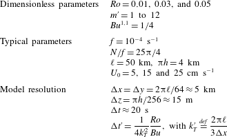
Table 1 outlines the parameter set explored. In a nutshell, simulations span non-dimensional vertical wavenumbers
 $m^{\prime }=1$
to 12, and three Rossby numbers. To fix ideas, the bottom entries of the table give one possible set of realistic dimensional parameters corresponding to the above dimensionless parameters. Of course, any combination of parameters yielding a given dimensionless numbers set leads to the same YBJ and YBJ+ solution. This is made clear in the non-dimensional form of the YBJ+ equation. Using
 $\ell$
to scale
 $x$
and
 $y$
,
 $h$
to scale
 $z$
and
 $(\mathit{Bu}^{1,1}f)^{-1}$
to scale
 $t$
, the non-dimensional YBJ+ equation is
 $$\begin{eqnarray}\unicode[STIX]{x2202}_{t}\mathsf{L}^{\!+}A+\frac{\mathit{Ro}}{\mathit{Bu}^{1,1}}\left[J(\unicode[STIX]{x1D6F9},\mathsf{L}^{\!+}A)+\frac{\text{i}}{2}\triangle \unicode[STIX]{x1D6F9}\mathsf{L}^{\!+}A\right]+\frac{\text{i}}{2}\triangle A=0,\end{eqnarray}$$
where
 $\unicode[STIX]{x1D6F9}=\sin x\sin y$
and, since
 $N$
is constant,
 $$\begin{eqnarray}\mathsf{L}^{\!+}A=A_{zz}+{\textstyle \frac{1}{4}}\mathit{Bu}^{1,1}\triangle A.\end{eqnarray}$$
Once again, the plain YBJ version is obtained by removing the term
 ${\textstyle \frac{1}{4}}\mathit{Bu}^{1,1}\triangle A$
from the definition of
 $\mathsf{L}^{\!+}A$
. The above equation set highlights an important distinction between the two approximate models: YBJ only depends on the ratio
 $\mathit{Bu}^{1,1}/\mathit{Ro}$
, whereas YBJ+ depends on
 $\mathit{Bu}^{1,1}$
and
 $\mathit{Ro}$
independently. This signals a superior parameter sensitivity for YBJ+. We comment on this in § 4.6.
Key parameters of the numerical simulations.

The testing procedure goes as follows: the YBJ and YBJ+ versions of (4.5) and (4.6) are integrated over 50 inertial periods using the parameter set in table 1. The accuracy of the two models is then assessed by comparing their solutions to that of the non-hydrostatic Boussinesq model used by Asselin, Bartello & Straub (Reference Asselin, Bartello and Straub2018). To put emphasis on the models rather than numerics, all three equation sets are integrated using the same numerical methods and parameters (cf. table 1). That is, the YBJ, YBJ+ and BQ models are pseudo-spectral, allowing horizontal derivatives to be computed with spectral accuracy. The
 $2/3$
rule is used to remove aliased modes. Vertical derivatives are approximated with second-order centred finite differences. Time integration is accomplished with the leap-frog scheme with a diffusion parameter
 $\unicode[STIX]{x1D6FE}=10^{-2}$
(Asselin Reference Asselin1972). To facilitate comparison between the models, no spatial diffusion is applied (except in a supporting simulation in § 4.5). Both temporal and vertical resolution were increased to convergence to eliminate them as sources of error. Horizontal resolution is much lower than vertical resolution to allow explicit treatment of the dispersive term for both YBJ and YBJ+. Indeed, with a horizontal resolution of
 $64\times 64$
, explicit treatment of the dispersive term in plain YBJ requires a time step of only 20 s. We verified that results below are unchanged as horizontal resolution is increased.
4.2 Overview comparison of YBJ and YBJ+
In both YBJ and YBJ+ the wave kinetic energy, estimated using the leading-order term in the expansion (2.28), is
 $$\begin{eqnarray}\text{WKE}\stackrel{\mathit{def}}{=}{\textstyle \frac{1}{2}}|\mathsf{L}\,A|^{2}.\end{eqnarray}$$
To assess the error relative to the Boussinesq solution we introduce
 $$\begin{eqnarray}E(t)\stackrel{\mathit{def}}{=}\sqrt{\frac{\langle (\text{WKE}-\text{WKE}_{BQ})^{2}\rangle }{\langle \text{WKE}_{BQ}^{2}\rangle }}.\end{eqnarray}$$
Above, the brackets
 $\langle \,\rangle$
indicate spatial averaging over the horizontal coordinates and subscript BQ indicates the solution of the Boussinesq solutions. The error is independent of the vertical level because WKE and
 $\text{WKE}_{BQ}$
share the same vertical structure.
(We emphasize that to define WKE for YBJ+ we use
 $\mathsf{L}$
, not
 $\mathsf{L}^{\!+}$
, in (4.7). We have verified by examination of the numerical solutions that the difference between
 $\mathsf{L}\,A$
and
 $\mathsf{L}^{\!+}A$
is small and thus there are only small differences between the two definitions of WKE. Moreover, the discussion following (3.2) provides a physical rationale in support of (4.7):
 $|\mathsf{L}^{\!+}A|^{2}$
contains a term corresponding to NIW potential energy.)
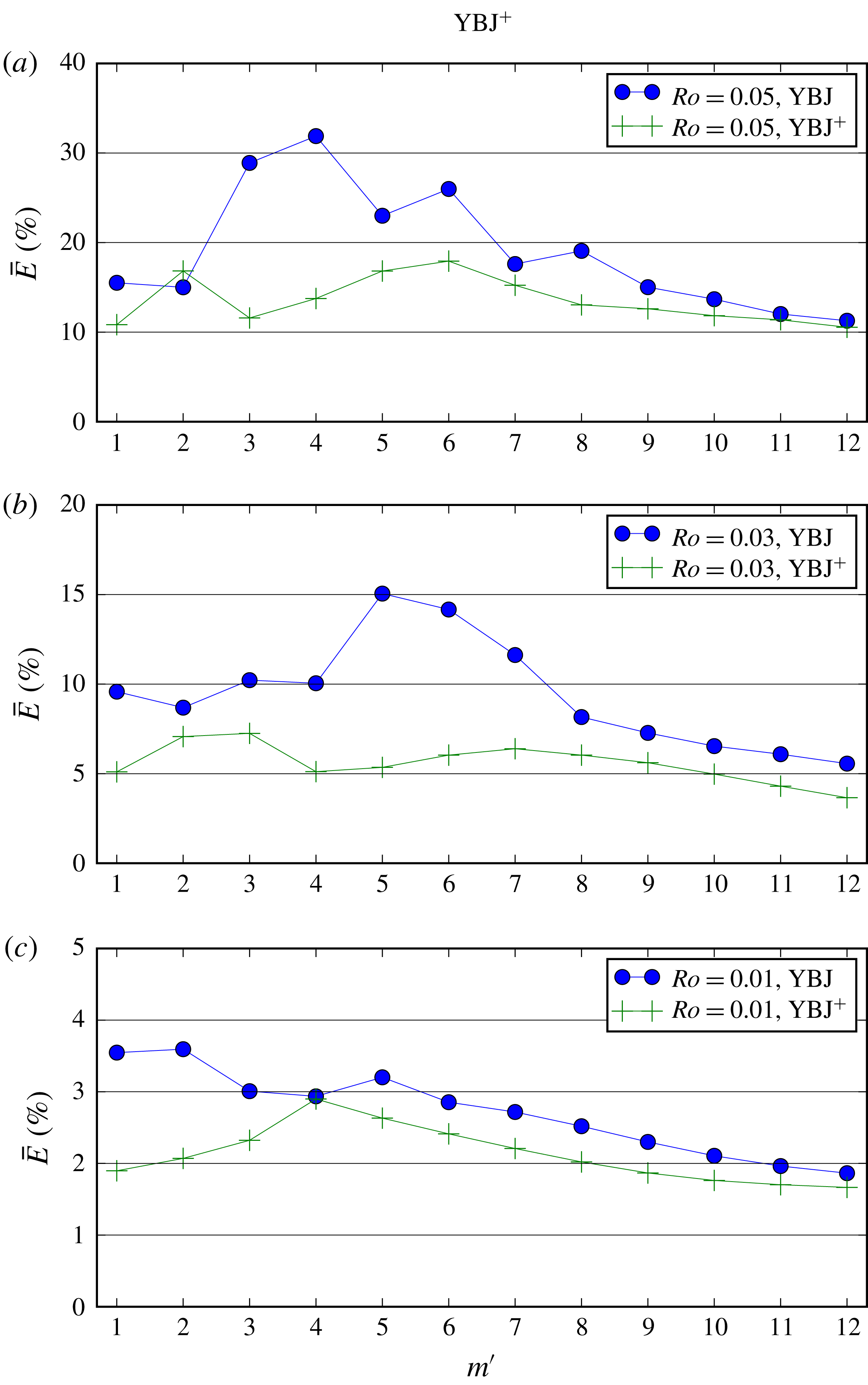
Figure 2 shows
 $\bar{E}$
, the
 $E(t)$
time averaged over the first 50 inertial periods of integration. The error is plotted against
 $m^{\prime }$
for the three Rossby numbers (one for each panel). In virtually all cases YBJ+ is more accurate that YBJ, as one would expect from the superior accuracy of YBJ+. Furthermore, for fixed
 $m^{\prime }$
the error decreases monotonically with
 $\mathit{Ro}$
for both models. In the lowest
 $\mathit{Ro}$
case (bottom panel), both models are accurate with just a few per cent error. This is consistent with the improved accuracy of their formal expansion as
 $\mathit{Ro}\rightarrow 0$
.
Error in WKE, defined in (4.8), and averaged over the first 50 inertial periods. Each marker represents a different simulation, with blue dots and green pluses for the error in the YBJ and YBJ+ models, respectively. Each panel has a fixed Rossby number.

The error dependence on
 $m^{\prime }$
is more puzzling. With increasing
 $m^{\prime }$
in the initial condition (4.1), the wave Burger number
 $\mathit{Bu}$
in (1.1) decreases as
 $m^{\prime -2}$
. The formal expansion indicates that both YBJ and YBJ+ become more accurate as
 $\mathit{Bu}$
is reduced. One might thus expect that the error in figure 2 should decrease monotonically and rapidly with increasing
 $m^{\prime }$
. In fact the dependence of error on
 $m^{\prime }$
in figure 2 is non-monotonic. Moreover, while the error does eventually decrease monotonically for large
 $m^{\prime }$
, this decrease is quite slow. To understand, or at least rationalize, the non-intuitive dependence of error on
 $m^{\prime }$
, we examine two illustrative cases: one with low (
 $m^{\prime }=1$
) and one with high (
 $m^{\prime }=8$
) vertical wavenumber.
4.3 A detailed look at the case
$m^{\prime }=1$
,
$\mathit{Ro}=0.05$
and
$\mathit{Bu}^{1,1}=1/4$


We first examine the case that one would naively assume to be most challenging: the solution with
 $\mathit{Ro}=0.05$
,
 $\mathit{Bu}^{1,1}=1/4$
and
 $m^{\prime }=1$
. In this strongly dispersive case, it is useful to introduce the parameter
 $$\begin{eqnarray}\unicode[STIX]{x1D702}\stackrel{\mathit{def}}{=}m^{\prime 2}\frac{\mathit{Ro}}{\mathit{Bu}^{1,1}}.\end{eqnarray}$$
In the limit
 $\unicode[STIX]{x1D702}\rightarrow 0$
, the YBJ+ equation (4.5) can be solved perturbatively with the initial condition in (4.1) (Young & Ben Jelloul Reference Young and Ben Jelloul1997; Thomas et al.
Reference Thomas, Smith and Bühler2017). For YBJ+ this solution is
 $$\begin{eqnarray}A=\text{e}^{\text{i}\unicode[STIX]{x1D714}t}[1+\unicode[STIX]{x1D702}(1-\text{e}^{-\text{i}\unicode[STIX]{x1D6FA}t})\sin x\sin y+\text{ord}(\unicode[STIX]{x1D702}^{2})]\cos (m^{\prime }z),\end{eqnarray}$$
where
 $$\begin{eqnarray}\unicode[STIX]{x1D6FA}\stackrel{\mathit{def}}{=}\frac{2}{2m^{\prime 2}+\mathit{Bu}^{1,1}},\quad \text{and}\quad \unicode[STIX]{x1D714}\stackrel{\mathit{def}}{=}\frac{2m^{\prime 2}+\mathit{Bu}^{1,1}}{8}\left(\frac{\mathit{Ro}}{\mathit{Bu}^{1,1}}\right)^{2}.\end{eqnarray}$$
(In their ‘strong dispersion regime’, TSB considered an asymptotic limit of the rotating shallow-water equations in which the Burger number is fixed and of order unity, while the Rossby number limits to zero. The more exact TSB version of (4.10) has the same structure: the leading-order term is a spatially uniform near-inertial oscillation and the higher-order terms contain the spatial dependence of the solution.)
The wave kinetic energy of the
 $\unicode[STIX]{x1D702}\ll 1$
solution in (4.10) is
 $$\begin{eqnarray}\text{WKE}(t)=\text{WKE}(0)[1+2\unicode[STIX]{x1D702}(1-\cos \unicode[STIX]{x1D6FA}t)\sin x\sin y+O(\unicode[STIX]{x1D702}^{2})].\end{eqnarray}$$
The YBJ version of (4.12) is obtained by neglecting
 $\mathit{Bu}^{1,1}$
relative to
 $2m^{\prime 2}$
in the definition of
 $\unicode[STIX]{x1D6FA}$
above. In the present case
 $\unicode[STIX]{x1D702}=0.2$
and (4.12) predicts
 $\text{WKE}(t)$
has modulations with amplitude reaching 80 % of the initial level
 $\text{WKE}(0)$
. This modulation has the same horizontal structure as the streamfunction (or vorticity, since in this case
 $\triangle \unicode[STIX]{x1D6F9}=-2\unicode[STIX]{x1D6F9}$
). Indeed, the effect of the refractive term
 $\triangle \unicode[STIX]{x1D6F9}\mathsf{L}^{\!+}A$
in (4.5) is to imprint the length scale of
 $\triangle \unicode[STIX]{x1D6F9}$
onto the wave field. Now the squared horizontal wavenumber of
 $\unicode[STIX]{x1D6F9}$
is 2 and therefore, although the domain-scale Burger number is
 $\mathit{Bu}^{1,1}={\textstyle \frac{1}{4}}$
, the effective Burger number of the NIW immediately after this initial imprinting is
 $$\begin{eqnarray}\mathit{Bu}_{init}={\textstyle \frac{1}{2}}.\end{eqnarray}$$
The formal expansion used to derive both YBJ and YBJ+ assumes that
 $\mathit{Bu}\ll 1$
and thus this test with an initial Burger number
 $1/2$
should be challenging.
Case:
 $m^{\prime }=1$
,
 $\mathit{Ro}=0.05$
and
 $\mathit{Bu}^{1,1}=1/4$
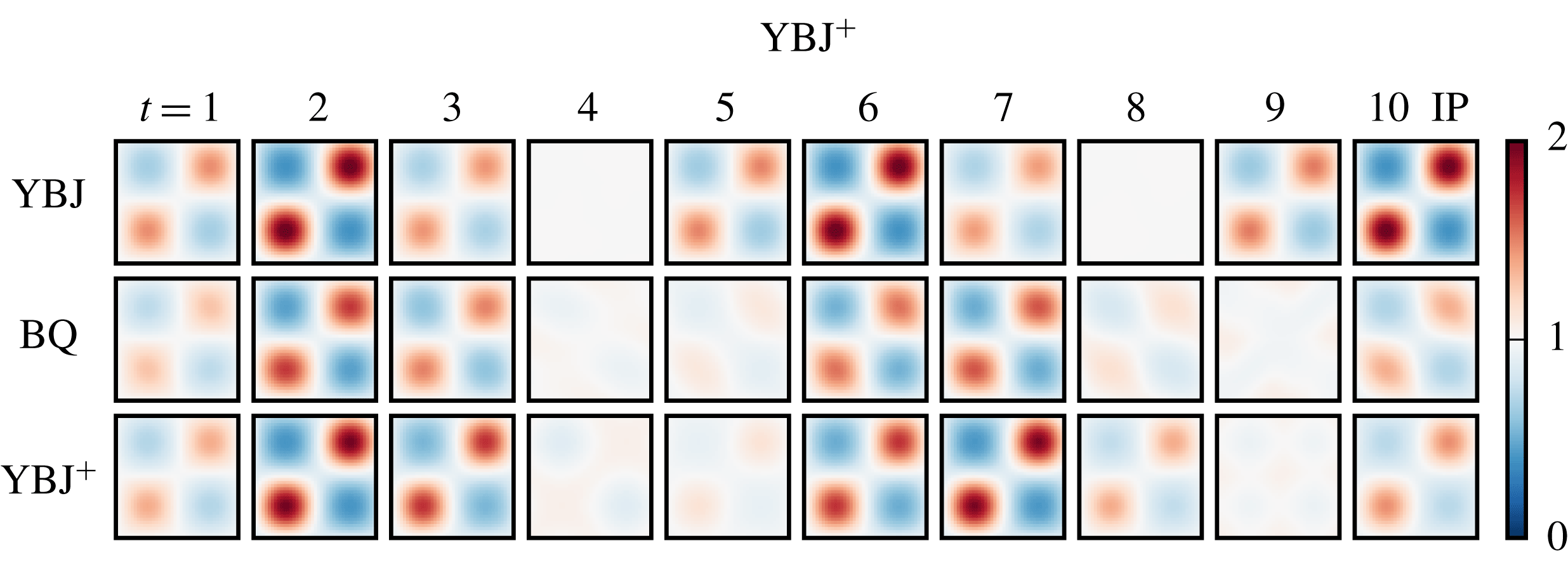
. Distribution of normalized wave kinetic energy as predicted by the YBJ, YBJ+ and Boussinesq (BQ) models at intervals of one inertial period (IP).

Figure 3 displays the horizontal distribution of wave kinetic energy in the first ten inertial periods of integration. Each row is associated with one of the three models, with the middle row BQ regarded as truth. These numerical solutions are broadly consistent with the asymptotic solution, (4.12). First, wave energy concentrates in regions of negative vorticity, i.e. following the predicted spatial structure
 $\sin x\sin y$
in (4.12). YBJ predicts that the period of the oscillation,
 $2\unicode[STIX]{x03C0}/\unicode[STIX]{x1D6FA}$
, is 4 inertial periods (IP); YBJ+predicts 4.5 IP. Figure 3 shows that the YBJ+ prediction is closer to the period of the Boussinesq solution. Finally, (4.12) predicts a modulation reaching
 $4\unicode[STIX]{x1D702}=80\,\%$
of
 $\text{WKE}(0)$
, which is comparable to that of the BQ solution. We verified that both YBJ and YBJ+ become more accurate as
 $\mathit{Ro}\rightarrow 0$
(and thus
 $\unicode[STIX]{x1D702}\rightarrow 0$
).
Case:
 $m^{\prime }=1$
,
 $\mathit{Ro}=0.05$
and
 $\mathit{Bu}^{1,1}=1/4$
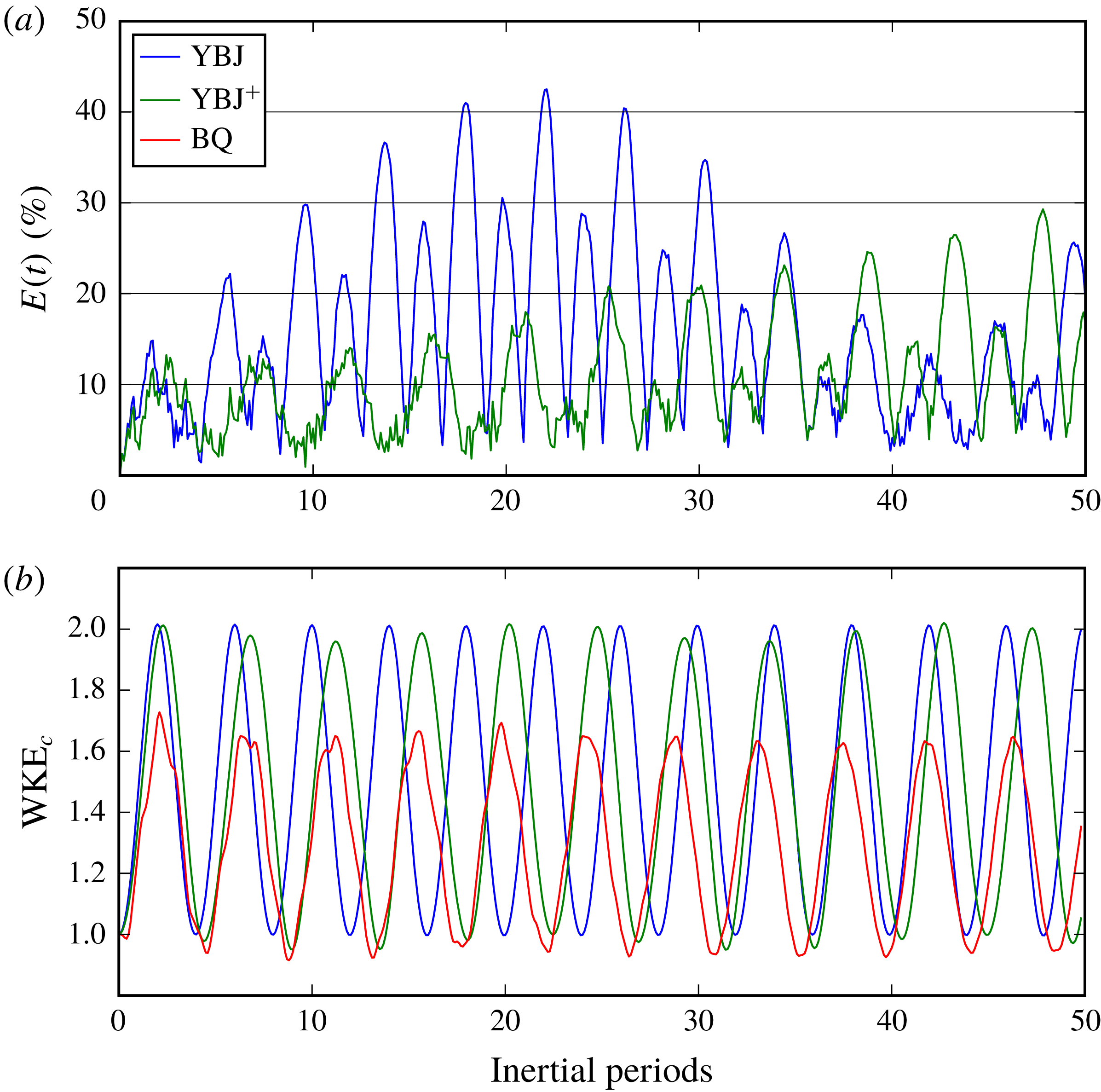
. (a) Time series of the error, (4.8), for both YBJ (blue) and YBJ+ (green) models. (b) Time series of the wave kinetic energy density at the core of the bottom left quarter for YBJ (blue), YBJ+ (green) and Boussinesq (BQ, red) solutions.

Although the overall horizontal structure of the BQ solution is well captured by the YBJ and YBJ+ models, the amplitude of the YBJ/YBJ+ oscillation is roughly 50 % larger than that of the BQ solution. This can be appreciated in the bottom panel of figure 4, which displays the time series of WKE at one of its maxima, the centre of the bottom left quarter,
 $x^{\prime }=y^{\prime }=\unicode[STIX]{x03C0}/2$
. YBJ and YBJ+ equally overestimate the amplitude of the BQ oscillation and miss some of its detailed structure. The plain YBJ solution also quickly shifts out of phase with the BQ solution. By comparison, YBJ+ predicts the phase of the oscillation significantly better than YBJ, as expected from its more accurate dispersion relation. This is reflected by an overall smaller error for YBJ+ during most of the integration (cf. figure 4
a), until the YBJ solution coincidentally comes back into phase after 40 inertial periods.
To recap, in this challenging high-
 $\mathit{Ro}~m^{\prime }=1$
case, WKE undergoes a weak modulation whose horizontal structure is well captured by both YBJ and YBJ+ models. The main source of error comes from an amplitude mismatch. YBJ+ captures the phase of oscillation much better than does YBJ, and this accounts for its higher accuracy.
4.4 A detailed look at case
$m^{\prime }=8$
,
$\mathit{Ro}=0.05$
and
$\mathit{Bu}^{1,1}=1/4$


Let us now turn our attention to a case with a larger vertical wavenumber,
 $m^{\prime }=8$
, keeping the Rossby number to its most challenging value,
 $\mathit{Ro}=0.05$
. Relative to the
 $m^{\prime }=1$
solution of figure 4,
 $m^{\prime }=8$
reduces the Burger number by a factor of 64: the analogue of (4.13) is an initially imprinted Burger number
 $$\begin{eqnarray}\mathit{Bu}_{init}={\textstyle \frac{1}{128}}.\end{eqnarray}$$
One expects that with this small Burger number, YBJ and YBJ+ should be more faithful to the BQ solution. Alas, the error summarized in figure 2 is not much less at
 $m^{\prime }=8$
than at
 $m^{\prime }=1$
.
Case:
 $m^{\prime }=8$
,
 $\mathit{Ro}=0.05$
and
 $\mathit{Bu}^{1,1}=1/4$
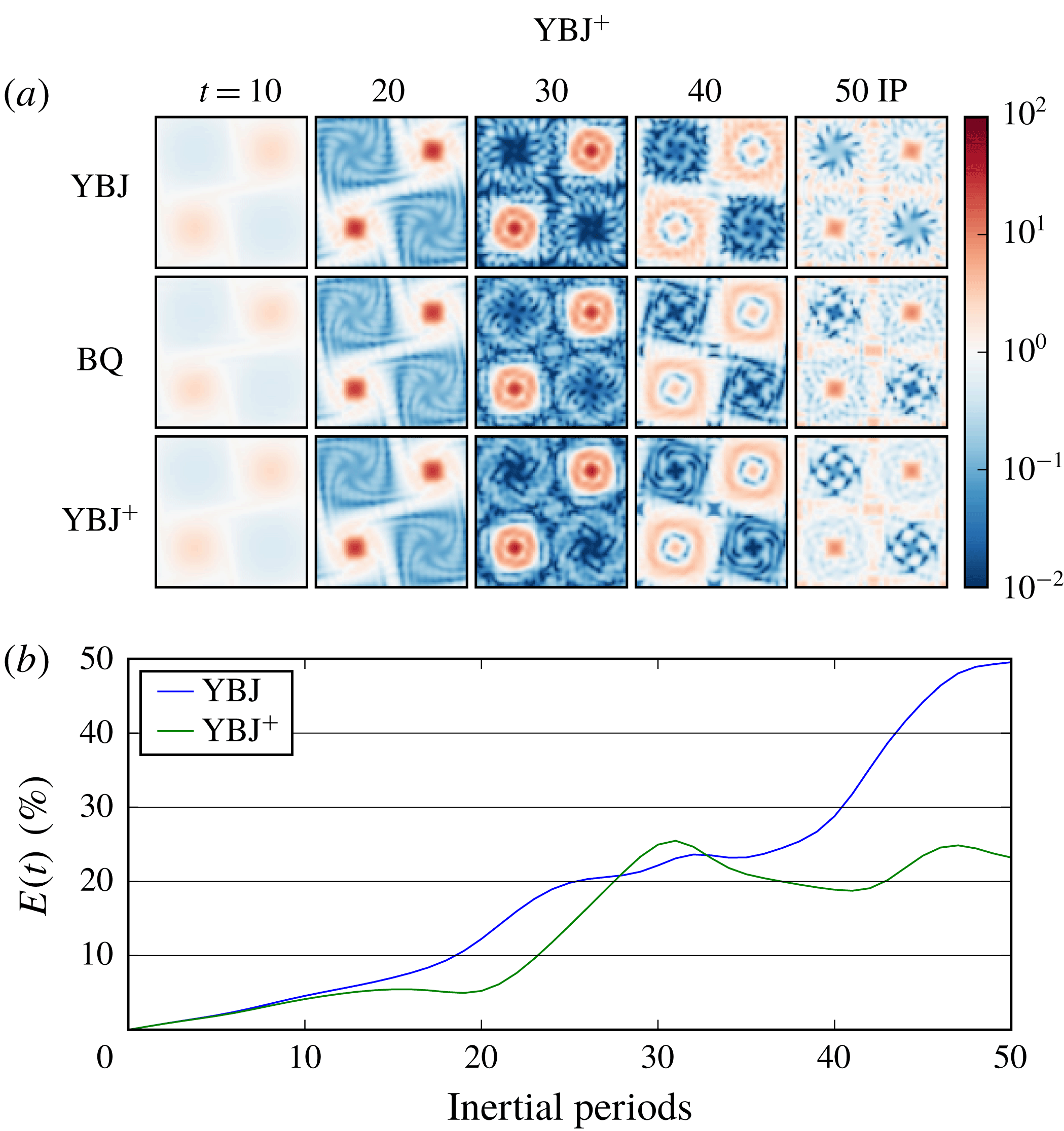
. (a) Normalized WKE distribution for the first 50 inertial periods of integration. A logarithmic scale is used to reveal both the fine-scale structure of the solution and the strong focussing of energy in the centre of negative vorticity cores. (b) Corresponding time series of error, equation (4.8).

To understand why, we refer to figure 5, which displays the horizontal WKE distribution (a) along with the associated error time series (b) for
 $m^{\prime }=8$
. As in the
 $m^{\prime }=1$
case, WKE initially concentrates in regions of negative vorticity. But there are two striking differences: (i) the anomaly is almost two orders of magnitude stronger: up to 3000 % as opposed to about 60 % in the
 $m^{\prime }=1$
case (note that a logarithmic scale is used for
 $m^{\prime }=8$
); (ii) the
 $m^{\prime }=8$
solution has a much finer horizontal structure. Because
 $\mathit{Bu}\propto k^{2}$
, a fine-scale structure implies that the effective
 $\mathit{Bu}$
is, in fact, much larger than the initially imprinted Burger number in (4.14). This crucial result deserves further discussion.
4.5 Evolution of effective Burger number
As shown above, a larger
 $m^{\prime }$
does not imply that
 $\mathit{Bu}$
remains small throughout the integration. As
 $m^{\prime }$
is increased,
 $\mathit{Bu}_{init}$
tends to zero and the dispersive term,
 $\text{i}\triangle A/2$
in (4.5), is initially very small relative to advection and refraction. Weakening dispersion results in the NIWs developing finer scale features, with higher horizontal wavenumber
 $k$
, and a larger effective
 $\mathit{Bu}\propto k^{2}$
. This rationalizes the slow decrease of error as
 $m^{\prime }$
is increased, but it also begs the question: does weakening dispersion fatally compromise the YBJ and YBJ+ models, which are based on the assumption of small
 $\mathit{Bu}$
? At least in our test computations, the answer is ‘no’ because dispersive wave propagation is effective in opposing advection and refraction.
Rocha, Wagner & Young (Reference Rocha, Wagner and Young2018) show that lateral straining increases the horizontal group velocity of NIWs so that the waves accelerate and escape from straining regions. This ‘wave escape’ ensures that NIWs do not suffer a forward cascade of action to the small horizontal scales on which dissipation is effective. In a flow that rapidly stirs passive scalar into diffusive oblivion, NIWs concentrate in vortex centres and wave action is robustly conserved, even as passive-scalar variance disappears in a few eddy turnover times.
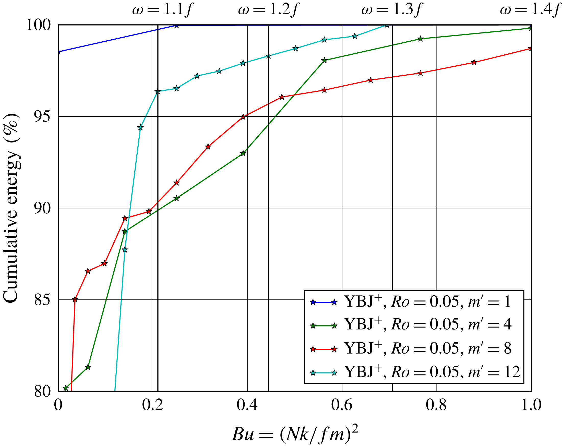
Cumulative wave energy as a function of the Burger number. The different colours represent YBJ+ solutions for different
 $m^{\prime }$
, all evaluated after 50 inertial periods. Horizontal wavenumbers are binned by integer steps, and therefore the spacing between points in
 $\mathit{Bu}$
thus depends on
 $m^{\prime }$
.

As evidence that wave escape is operating in our solutions, figure 6 shows the cumulative distribution of wave energy,
 ${\textstyle \frac{1}{2}}|\mathsf{L}^{\!+}A|^{2}$
, as a function of the Burger number. That is, the ordinate at a given
 $\mathit{Bu}$
corresponds to the sum of wave energy at all Burger numbers equal to or smaller than
 $\mathit{Bu}$
. Remarkably, the case
 $m^{\prime }=1$
actually contains less energy at
 $\mathit{Bu}\sim 1$
than all other cases, including
 $m^{\prime }=8$
. Indeed, in the former case more of the energy remains in the
 $k^{\prime }=0$
mode, or equivalently, oscillations of the solution have a much weaker amplitude. In that sense, the effective
 $\mathit{Bu}$
for
 $m^{\prime }=8$
is more challenging than for
 $m^{\prime }=1$
, even though
 $\mathit{Bu}_{init}$
at
 $m^{\prime }=8$
is 64 smaller than at
 $m^{\prime }=1$
.
The numerical size of
 $\mathit{Bu}$
is important in this discussion. Suppose that the initial
 $\mathit{Bu}_{init}$
is very small, say
 $1/128$
. If advection increases the effective
 $\mathit{Bu}$
to
 $1/5$
, then that is a large increase relative to
 $\mathit{Bu}_{init}=1/128$
. But waves with
 $Bu=1/5$
have
 $\unicode[STIX]{x1D714}=1.09\,f$
and are therefore still near inertial. Thus it is striking that in figure 6 the range
 $0\leqslant \mathit{Bu}\leqslant 0.2$
contains at least 90 % of wave energy for all
 $m^{\prime }$
shown. This also means that 90 % of waves oscillate with a frequency between
 $f$
and
 $1.09\,f$
. The amount of energy above
 $\mathit{Bu}=1$
(equivalently above
 $1.4\,f$
) is minute, reaching a maximum of approximately 2 % in the case
 $m^{\prime }=8$
. Thus although small horizontal scales are created by advection and refraction, and although there is a very large increase in
 $\mathit{Bu}$
relative to
 $\mathit{Bu}_{init}$
, the amount of energy reaching Burger numbers large enough to challenge YBJ+, such as
 $\mathit{Bu}=1$
in figure 1, is small.
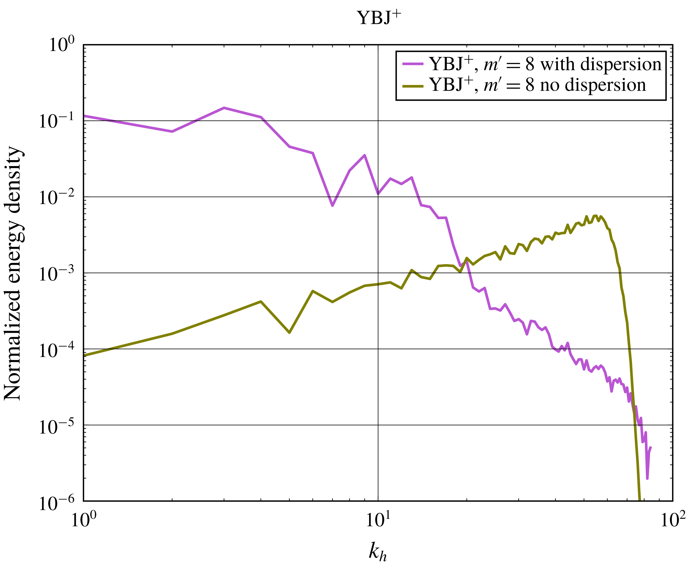
We emphasize that although dispersion becomes weak at high
 $m^{\prime }$
, it is by no means negligible. Figure 7 illustrates this point by showing equilibrium wave energy spectra for YBJ+ at
 $m^{\prime }=8$
and
 $\mathit{Ro}=0.05$
, with and without the dispersive term
 $\text{i}\triangle A/2$
in (4.5). For these simulations only, the resolution was increased to
 $256^{3}$
and a small amount of hyperdiffusion was included to smooth small horizontal scales. The cases with and without dispersion are strikingly different. In the absence of dispersion (green), wave energy tends to equipartition between all the available modes, approaching a
 $k^{1}$
spectrum till an abrupt hyperdiffusive cutoff. In other words, without the small dispersive term, large scales are rapidly purged of their energy, which cascades to smaller scales. But with small dispersive case (purple) energy remains at larger scales with small
 $\mathit{Bu}$
. After a few hundred inertial periods, more than 90 % of the initial energy remains, whereas about only 10 % remains in the case without dispersion. (We have verified that these results are robust to changes in resolution and the strength of the hyperdiffusion coefficient.)
Wave energy spectra as a function horizontal wavenumber. YBJ+ solutions with
 $Ro=0.05$
and
 $m^{\prime }=8$
are shown with (purple) and without (olive) dispersion. Spectra are captured at equilibria after 300 inertial periods, and are averaged over the 50 surrounding inertial periods. The spectra are normalized so that the initial condition sums to unity. These simulations have the same parameters as in the rest of this paper, except that the resolution is
 $256^{3}$
and hyperdiffusion was added to remove small horizontal scales.

4.6 Dimensional reduction of the parameter space
The non-dimensional equation set (4.5) and (4.6) also deserves further discussion. For a fixed initial condition, the solution of a given equation system, YBJ, YBJ+ or BQ, is uniquely defined by its set of dimensionless numbers. For instance, the solution of the inviscid non-hydrostatic Boussinesq equations is determined by three control parameters:
 $\mathit{Ro}$
,
 $\mathit{Bu}$
and
 $Ar$
, where
 $Ar$
is the aspect ratio. That is, for a fixed initial condition, there is only one solution associated with each point of the cube of dimensions
 $\mathit{Ro}\times \mathit{Bu}\times Ar$
. Both the YBJ and YBJ+ model assume hydrostatic balance, which imply
 $Ar\rightarrow 0$
: the space of possible solutions shrinks to a
 $\mathit{Ro}$
–
 $\mathit{Bu}$
plane. Furthermore, (4.5) and (4.6) highlight that YBJ in fact only depends on Burger-to-Rossby ratio, and thus admits only one solution per straight line in the
 $\mathit{Bu}$
–
 $\mathit{Ro}$
plane. This was appreciated by Thomas et al. (Reference Thomas, Smith and Bühler2017), who defined their various dispersion regimes based on the slope of the line crossing the
 $\mathit{Bu}$
–
 $\mathit{Ro}$
plane (cf. their figure 3).
Normalized wave kinetic energy density at the surface,
 $m^{\prime }=6$
, for the three models (three rows). Each column displays a solution with a different set of
 $\mathit{Ro}$
and
 $\mathit{Bu}^{1,1}$
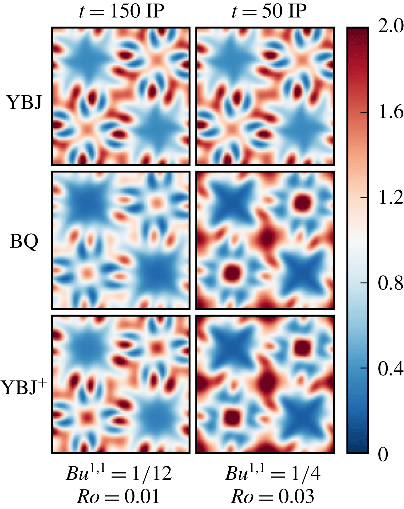
, but with their ratio held fixed. As such, when time is appropriately stretched the YBJ model has the same output (upper panels). On the other hand, the output of the Boussinesq and YBJ+ models are influenced by the independent changes in
 $\mathit{Ro}$
and
 $\mathit{Bu}^{1,1}$
.

YBJ+ has more degrees of freedom than YBJ: YBJ+ is sensitive to
 $\mathit{Bu}$
and
 $\mathit{Ro}$
independently. This is illustrated in figure 8. As usual, the three rows are associated with the three models. But instead of showing a time series from left to right, figure 8 shows snapshots from two simulations with different Rossby and Burger numbers but fixed
 $\mathit{Bu}^{1,1}/\mathit{Ro}$
. Here, the right panel has its Burger and Rossby numbers multiplied by 3, and is thus shown at a dimensional time divided by 3. As expected, the YBJ solution is the same in both cases. However, both BQ and YBJ+ change rather importantly between the two cases, leaving YBJ behind. Unsurprisingly, YBJ+ does better as
 $\mathit{Bu}$
and
 $\mathit{Ro}$
are increased while keeping their ratio fixed.
5 Conclusion
In this contribution we have introduced YBJ+, an improved model for the evolution of near-inertial waves in a geostrophic flow. The YBJ+ equation is obtained by replacing the operator
 $\mathsf{L}$
with
 $\mathsf{L}^{\!+}=\mathsf{L}+{\textstyle \frac{1}{4}}\triangle$
throughout the YBJ equation. Compared with its predecessor, YBJ+ brings the twin advantages of superior accuracy and numerical expediency whilst maintaining ease of implementation.
The YBJ+ dispersion relation is second-order accurate in
 $\mathit{Bu}$
and is therefore much more accurate than that of YBJ. This improvement results in a significant reduction of phase error (e.g. figure 4). Furthermore, while YBJ depends solely on the ratio
 $\mathit{Ro}/\mathit{Bu}$
, YBJ+ depends on
 $\mathit{Ro}$
and
 $\mathit{Bu}$
independently. This superior parameter sensitivity allows YBJ+ to track the Boussinesq solution over a wider region of parameter space (see figure 8). YBJ+ is more accurate than YBJ in virtually all cases we considered (see figure 2). Compared with the second-order accurate model proposed by TSB, YBJ+ is a Padé approximant to the exact dispersion relation, yielding superior accuracy for near-unity
 $\mathit{Bu}$
(see figure 1).
Aside from this gain in accuracy, YBJ+ requires less computational effort. The time step required for a stable explicit integration of YBJ decreases proportionally with horizontal resolution. In practical applications the YBJ equation can thus only be solved with an implicit time-stepping scheme, which necessarily distorts high-frequency waves. On the other hand, in YBJ+ the frequency of waves asymptotes to
 $2f$
at high horizontal wavenumbers. One can thus conveniently integrate the dispersive term with an explicit scheme and a reasonable computational effort. We also remark that YBJ+ is readily implemented from an existing YBJ model: the algorithm for the
 $\mathsf{L}^{\!+}A\rightarrow A$
inversion is the same as for the
 $q\rightarrow \unicode[STIX]{x1D713}$
inversion required in a quasi-geostrophic model.
The main appealing features of YBJ are preserved in the improved version. First and foremost, YBJ+ only requires a time scale separation between the geostrophic flow and the waves; no spatial scale separation is required. The processes of advection, refraction and dispersion are each conveniently associated with a different term in the equation. YBJ+ also enjoys conservation laws analogue to YBJ (see § 3).
The numerical test of YBJ+ in § 4 forced us to confront some facts of NIW life. In particular, we found that the YBJ and YBJ+ errors do not decrease monotonically with
 $\mathit{Bu}_{init}$
(or
 $m^{-1}$
; see figure 2). This is surprising: one expects YBJ and YBJ+ to become more accurate as
 $\mathit{Bu}_{init}$
tends to zero. With closer examination we found that as a result of advection and refraction, solutions with higher
 $m$
develop finer-scale horizontal structure so the effective
 $\mathit{Bu}\propto k^{2}$
becomes larger than the initial Burger number
 $\mathit{Bu}_{init}$
. In other words, even if
 $\mathit{Bu}_{init}$
is very small, advection and refraction attack the approximation by increasing
 $\mathit{Bu}$
. The approximation is rescued by small, but non-negligible, dispersion that successfully opposes advection and refraction and confines most of the NIW energy to relatively large scales and low
 $\mathit{Bu}$
(see figure 6). We conclude by recommending the use of YBJ+ over YBJ as a phase-averaged model of near-inertial wave dynamics.
Acknowledgements
This work was supported by the National Science Foundation Award OCE-1657041. We thank S. Smith, J. Vanneste, J.-H. Xie and anonymous referees for comments and advice that greatly improved this work.