1 Introduction
The emission of sound waves in a liquid is known to be an efficient way to set a fluid in motion. In a first mechanism, explained by Eckart (Reference Eckart1948), streaming mainly occurs in the bulk due to viscous attenuation. In a second mechanism, observed even in low-dissipation fluids, streaming takes its origin near boundaries where velocity gradients are the strongest and can drive fluid circulations up to the bulk (Westervelt Reference Westervelt1953; Holtsmark et al. Reference Holtsmark, Johnsen, Sikkeland and Skavlem1954). In microfluidic geometries, acoustic streaming is often considered as one way to generate vorticity and subsequent mixing in flows dominated by viscous forces. To obtain significant flow velocities, strong acoustic sources can be used, as is the case with bulk acoustic wave resonators or systems involving surface acoustic waves (Friend & Yeo Reference Friend and Yeo2011; Lei, Hill & Glynne-Jones Reference Lei, Hill and Glynne-Jones2014). Alternatively, the use of bubbles can give rise to intense streaming in the surrounding liquid, since, when excited at its resonant frequency, the gas/liquid interface of the bubble can strongly vibrate (Leighton Reference Leighton1994). In the extreme case of collapsing bubbles, the violent flows generated by the bubble vibration can even damage the neighbouring surfaces.
Elder (Reference Elder1958), Marmottant & Hilgenfeldt (Reference Marmottant and Hilgenfeldt2003) and Tho, Manasseh & Ooi (Reference Tho, Manasseh and Ooi2007) performed various experiments with nearly spherical bubbles attached to a wall with a finite contact angle. They observed strong microstreaming when the bubble was excited near resonance, with vorticity affecting particle trajectories at distances exceeding 10 bubble radii. Longuet-Higgins (Reference Longuet-Higgins1997) explained that intense long-range vorticity results from the combination of two modes of vibration oscillating out of phase. These two modes are in their case the main volume mode and the to-and-fro translation of the bubble centre of mass with respect to the solid surface. In such mixed-mode streaming, the near-boundary streaming velocity is of the order of
 $U_{s}^{n,m}={\it\epsilon}_{n}{\it\epsilon}_{m}R_{0}{\it\omega}_{d}\sin ({\rm\Delta}{\it\phi}^{n,m})$
, where
 ${\it\epsilon}_{n,m}$
is the relative amplitude of each mode and
 ${\rm\Delta}{\it\phi}^{n,m}$
is the phase shift between the two modes, and where
 $R_{0}$
and
 ${\it\omega}_{d}$
stand for the bubble radius and driving frequency. Interestingly, this theory, developed for freely oscillating spherical bubbles (see Davidson & Riley Reference Davidson and Riley1971; Wu & Du Reference Wu and Du1990; Doinikov & Bouakaz Reference Doinikov and Bouakaz2010, for more details), found application in other experiments by Ahmed et al. (Reference Ahmed, Mao, Juluri and Huang2009a
,Reference Ahmed, Mao, Shi, Juluri and Huang
b
, Reference Ahmed, Chan, Lin, Muddana, Nama, Benkovic and Huang2013), Wang, Jalikop & Hilgenfeldt (Reference Wang, Jalikop and Hilgenfeldt2012) and Wang, Rallabandi & Hilgenfeldt (Reference Wang, Rallabandi and Hilgenfeldt2013). In these cases, the bubble sticks out from a slit that extends between the walls of a microfluidic channel, leading to a semicylindrical liquid/air interface. Large amplitudes of vibration are obtained when the excitation frequency corresponds to a perimeter that is a multiple of the Faraday wavelength. These non-parametric Faraday modes can combine with the resonant volume mode, leading to ‘fountain’ vortices at low driving frequencies. The near-boundary counter-rotating ‘anti-fountain’ vortices induced by the presence of the channel wall finally take over the ‘fountain’ vortices on increasing the driving frequency (Wang et al.
Reference Wang, Rallabandi and Hilgenfeldt2013; Rallabandi, Wang & Hilgenfeldt Reference Rallabandi, Wang and Hilgenfeldt2014). Again, a mixed-mode streaming explanation, adapted to take into account the peculiarities of the boundary conditions, seemed to capture most experimental observations.
In the present work, we study the microstreaming that develops around bubbles squeezed between the two walls of a microfluidic channel and positioned close enough to interact and give rise to a novel type of mixed-mode streaming. In § 2, we describe the experimental conditions under which we generate and observe acoustic streaming from bubbles. We present in § 3 the experimental streaming patterns observed in various conditions. In order to understand the origin of the different patterns, we provide in § 4 a theoretical study of the vibration modes that appear for a pair of bubbles, considering their interaction through the microchannel walls. In § 5, we then develop a model of mixed-mode acoustic streaming for two near-resonant acoustic bubbles. Various regimes are then evidenced and reproduced via numerical simulations. In § 6, we detail the mean flow velocity field in the specific case of two bubbles put into contact and compare the experiments to the model. We finally conclude in § 7 on some consequences on the control of microscale flows.
2 Materials and methods
2.1 Experimental set-up
A silicone (polydimethylsiloxane, PDMS) microfluidic chip was built using soft-lithography techniques to produce and study in situ gas bubbles. First, we inject nitrogen and water in a flow-focusing orifice, producing monodisperse microbubbles. A commercial dishwashing detergent (Dreft, Procter and Gamble) is added to the water in order to get a thin wetting film between the channel wall and the bubbles. In the following, we assume that the resulting liquid has the same density and viscosity as water and thus will be considered as a Newtonian fluid. With this technique, bubbles with radii
 $R_{0}$
ranging between
 $20$
and
 $70~{\rm\mu}\text{m}$
are obtained, their size depending on the liquid flow rate and the gas pressure. After production, bubbles are released in a wide (
 $w=2.17~\text{mm}$
) and thin (
 $h_{0}=25~{\rm\mu}\text{m}$
) channel and flow over small micropits (
 $40~{\rm\mu}\text{m}$
in height and
 $d=40~{\rm\mu}\text{m}$
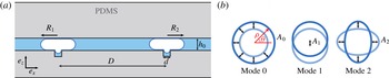
in diameter) patterned on one side of the channel walls, according to the technique developed by Abbyad et al. (Reference Abbyad, Dangla, Alexandrou and Baroud2011). As long as the drag force applied by the surrounding fluid is low enough, the bubbles may get trapped on the micropits. Each bubble enters partially into a hole, leading to the situation sketched on figure 1(a), and, since
 $d/h_{0}\leqslant 2$
, its deformation leads to a decrease of its surface energy (Dangla, Lee & Baroud Reference Dangla, Lee and Baroud2011). With this procedure, one, two or several bubbles can be stopped or removed at will, with relative distances set by the micropit arrangement.
Bubble oscillations are then obtained by vibrating a piezo-transducer glued on a glass bar encased into the PDMS polymer. Because the thickness of the glass bar is only 1 mm, surface waves (called Lamb waves) are excited on the glass surface. The length of the glass bar is adjusted in order to get principally a standing Lamb wave. The acoustic wave then propagates through
 $150~{\rm\mu}\text{m}$
of PDMS before exciting the bubble. The driving frequency
 ${\it\omega}_{d}$
is chosen in the range of 50–200 kHz and must be close enough to the resonant modes of the glass bar and to the bubble resonance in order to get perceptible oscillations of the bubbles. At these driving frequencies, the Lamb wavelength exceeds 4 mm. The distance between bubbles is then chosen much smaller than half the Lamb wavelength. The two bubbles are approximately placed close to a pressure antinode of the glass bar in order to excite both bubbles with a comparable amplitude and phase. Because the liquid stuck inside the micropit by the bubble is extremely confined, no vibration of the gas/liquid interface occurs inside the micropit: the bubble only vibrates in the channel plane.
(a) Scheme of the experimental set-up (sectional view): two flattened gas bubbles (white) are confined in a PDMS microchannel (grey) of height
 $h_{0}=25~{\rm\mu}\text{m}$
filled with water (blue) and are anchored on micropits of diameter
 $d=40~{\rm\mu}\text{m}$
. (b) Schematic representation of the first deformation modes (top view of the bubble contour): breathing mode
 $n=0$
, translation mode
 $n=1$
and quadrupolar mode
 $n=2$
.

Bubble motions are recorded using a fast camera (Miro 310, Vision Research) connected to an inverted microscope (Olympus, model IX70). Since the real-time dynamics exceeds the capability of the camera, the acquisition is triggered in a stroboscopic way, adjusting the camera frequency to slow down the evolution to 5 Hz. With this experimental arrangement, we are advantageously able to observe bubbles at preset positions while, as later verified, they are free to oscillate in the channel plane, allowing observations over periods of time that may exceed several minutes.
Last, the streaming around the bubbles is made visible by adding
 $3~{\rm\mu}\text{m}$
yellow-green fluorescent microbeads (Fluoresbrite, Polysciences Inc.) into the liquid. The estimated Stokes number
 $St={\it\rho}_{b}d_{b}^{2}U_{c}/{\it\mu}d_{c}$
(with
 ${\it\rho}_{b}$
and
 $d_{b}$
the bead density and diameter,
 ${\it\mu}$
the liquid dynamic viscosity and
 $U_{c}$
and
 $d_{c}$
the characteristic velocity and distance) stays below
 $0.1$
, meaning that these beads are good tracers in the bulk. Nevertheless, when the beads come into contact with the bubble wall, where the fluid velocity is maximal and the streamlines narrow, beads can deviate from their initial trajectory and follow a neighbouring streamline, as shown by Wang, Jalikop & Hilgenfeldt (Reference Wang, Jalikop and Hilgenfeldt2011).
2.2 Video analysis
2.2.1 Particle tracking velocimetry (PTV)
The particle trajectories around the bubbles were analysed using the trackmate plugin of the Fiji freeware (NIH, USA; see Rasband Reference Rasband2008) and were numerically processed. The density of tracers was optimized in order to reduce particle–particle interactions and improve the traceability of the particles. The successive positions of the beads, projected in the channel plane, were measured over tens of seconds to obtain significant statistics. Radial and tangential Lagrangian velocities were then derived from the position measurements of the tracers. We defined a typical mesh size of dimension
 $12~{\rm\mu}\text{m}\times 12~{\rm\mu}\text{m}$
, larger than the camera resolution. For each pixel of this new mesh, we calculated the averaged velocities. In order to minimize the tracking errors of the plugin, data were filtered by replacing the averaged velocities of the considered pixel by the average on the closest neighbouring pixels whenever the first one was more than three times higher than the latter. Velocity values in empty pixels were interpolated from the neighbouring pixel values using an inverse distance weighting interpolation with a power parameter of 2. Apart from these two occasional cases, pixel values were unchanged.
2.2.2 Vibration mode decomposition
In order to understand the link between the streaming observed around the bubbles and their deformation modes, an analysis of the bubble shape was conducted in parallel with the velocity measurements. For this purpose, we use for each bubble the coordinates introduced on figure 1(b). Since the bubbles are confined between two walls, they vibrate essentially in the channel plane. The contour
 ${\it\rho}({\it\theta},t)$
of each bubble in the channel plane can be decomposed in a Fourier series as
 $$\begin{eqnarray}\displaystyle {\it\rho}({\it\theta},t)=R_{0}+\mathop{\sum }_{n\geqslant 0}A_{n}\cos ({\it\omega}t+{\it\phi}_{n})\cos (n{\it\theta}+{\it\psi}_{n}), & & \displaystyle\end{eqnarray}$$
where
 $R_{0}$
is the average radius of the bubble,
 $A_{n}$
the amplitude of the mode
 $n$
,
 ${\it\omega}$
its oscillating frequency,
 ${\it\phi}_{n}$
its temporal phase shift with respect to the phase of the excitation and
 ${\it\psi}_{n}$
its spatial phase shift setting the angular orientation of the mode. We write
 $a_{n}(t)=A_{n}\cos ({\it\omega}t+{\it\phi}_{n})=\text{Re}(\overline{A}_{n}\text{e}^{\text{i}{\it\omega}t})$
, the time evolution of the mode amplitude. In practice, the bubble oscillation can be decomposed into a sum of a volume mode (also called breathing mode) of amplitude
 $A_{0}$
and higher-order modes (called surface modes). In the following, we will mainly discuss two surface modes: the mode
 $n=1$
describes the to-and-fro translation of the bubble; the mode
 $n=2$
is a quadrupolar mode where the bubble is elongated alternately in two perpendicular directions. These modes are schematically represented on figure 1(b).
3 Experimental results
3.1 Generation of extended streaming with a bubble pair
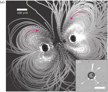
An example of the steady streaming observed around a single bubble is given on figure 2(a). In this example, the driving pressure exceeds the pressure threshold of the two-dimensional (2D) parametric instability (see Mekki-Berrada, Thibault & Marmottant Reference Mekki-Berrada, Thibault and Marmottant2016). In addition to its breathing mode, the bubble exhibits a parametric surface mode
 $n=4$
that can be identified by the
 $2n$
surface-mode antinodes on the bubble contour. The successive positions of the fluorescent particles have been superimposed to highlight the different possible trajectories in the surrounding liquid. One can distinguish two types of trajectories. The first one is an apparent back-and-forth motion that seems to occur perpendicularly to the channel plane and which is restricted to a short region around the bubble (typically one bubble diameter, here around
 $80~{\rm\mu}\text{m}$
). This trajectory appears even below the parametric instability threshold and is thus correlated to the volume pulsation. The second type of streaming appears in the vicinity of the bubble and is associated with the presence of the surface mode. It is characterized by in-plane vortices that scale like the surface-mode wavelength. In both cases, the vortices generated by the pulsation of the isolated bubble are limited in scope.
Comparison of the microstreaming generated by (a) a bubble pair and (b) a single bubble of respective radius
 $R_{0}=30~{\rm\mu}\text{m}$
and
 $R_{0}\simeq 25~{\rm\mu}\text{m}$
, acoustically exited at respectively
 $f_{d}=104~\text{kHz}$
and
 $f_{d}=148~\text{kHz}$
. The driving acoustic pressure is estimated to be around
 $p^{ac}=40~\text{kPa}$
. The flow is materialized by the superposition of images from a movie recording, showing the successive positions of
 $3~{\rm\mu}\text{m}$
fluorescent microbeads (white). The arrows materialize the in-plane flow directions. The scale bar is the same in both panels.

We found that placing a second bubble close to the first one greatly enhances the microstreaming. The two bubbles can be simultaneously excited and put in oscillation in either parametric or non-parametric mode. We show on figure 2(b) stack images of the flow generated by two bubbles at a distance apart of
 $280~{\rm\mu}\text{m}$
and excited below the parametric instability threshold. Compared to the single-bubble case, we obtained an extended streaming in the plane of the channel, the extension of which goes up to
 $450~{\rm\mu}\text{m}$
, forming a quadrupolar-like (‘butterfly’) steady flow oriented along the inter-bubble axis. The streaming velocities in the vicinity of each bubble are typically
 $3~\text{mm}~\text{s}^{-1}$
. The streaming trajectories in the vicinity of each bubble are complex because they combine the butterfly streaming pattern with the short-range streaming previously observed on the single bubble.
3.2 Modulation of the streaming intensity and streaming pattern
In the following, we focus on such bubble pairs and the characterization of the streaming they produce. This involves controlling the experimental conditions and the physical parameters that affect the bubble vibrations. In practice, by anchoring the bubbles on micropits, we are able to control their distance. We also checked that they are still free to oscillate thanks to the presence of surfactant in the liquid that leads to fully wetting conditions, and thus to a good lubrication with the walls. In this part, we concentrate on the microstreaming generated at low driving pressure, i.e. below the parametric instability threshold.
Streaming pattern around a bubble pair of radii
 $R_{0}=25~{\rm\mu}\text{m}$
excited at a frequency
 $f_{d}=80~\text{kHz}$
, for bubble distances of (a)
 $D=50~{\rm\mu}\text{m}$
(bubbles are in contact), (b)
 $D=150~{\rm\mu}\text{m}$
, (c)
 $D=200~{\rm\mu}\text{m}$
and (d)
 $D=250~{\rm\mu}\text{m}$
.

3.2.1 Influence of bubble separation
The influence of the distance on the microstreaming pattern has been qualitatively investigated, and figure 3 illustrates the main results. When the two bubbles are set into contact (figure 3 a), long-range streaming develops around the excited bubbles. By increasing step-by-step the distance between the two pinned bubbles while keeping the same bubble size, the streaming becomes less and less intense (figure 3 b–d). When the distance between the bubbles is much larger than their radii, the out-of-plane vortices observed on single bubbles reappear and the streaming becomes mainly three-dimensional (3D).
From these experiments, we see that two bubbles may give rise to long-range streaming, even when their distance exceeds that of their individual acoustic streaming. In addition, the vortices they produce seem to be linked to their respective distance
 $D$
. This clearly indicates the existence of an interaction distance between the two bubbles.
Rabaud et al. (Reference Rabaud, Thibault, Mathieu and Marmottant2011) indeed observed that the excitation of confined bubbles generates a surface (Rayleigh) wave that propagates on the PDMS walls, resulting in a radiation force that can be attractive or repulsive depending on the distance
 $D$
between the bubbles. The acoustic interaction potential associated to this force is minimal when
 $D$
is approximately a multiple of the Rayleigh wavelength. For a typical surface wave velocity of approximately
 $c_{R}=30~\text{m}~\text{s}^{-1}$
, this leads to equilibrium distances that are a multiple of
 ${\it\lambda}=c_{R}/f_{d}$
, ranging from
 ${\it\lambda}=150$
to
 $600~{\rm\mu}\text{m}$
using the previous values of
 $f_{d}={\it\omega}_{d}/2{\rm\pi}$
(between 50 and 200 kHz). Therefore, the ratio
 $D/{\it\lambda}$
seems to be one of the fundamental parameters of the bubble pair system, in addition to the ratio
 $R_{0}/{\it\lambda}\propto R_{0}f_{d}$
that quantifies the proximity to the bubble resonance.
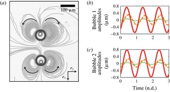
(a) Fountain streaming around a bubble pair of radii
 $R_{0}=35~{\rm\mu}\text{m}$
, separated by a distance
 $D=200~{\rm\mu}\text{m}$
and excited at a frequency
 $f_{d}=50~\text{kHz}$
. Black arrows represent the direction of the bead trajectories. (b,c) Amplitude
 $a_{n}(t)$
of the breathing mode (red solid line), the translational mode
 $n=1$
(orange dashed line) and the mode
 $n=2$
(green dotted line), for the two bubbles. The most excited mode is the mode
 $n=1$
and is out of phase with the breathing mode, with
 ${\rm\Delta}{\it\phi}^{(1,0)}={\it\phi}_{1}-{\it\phi}_{0}\simeq -{\rm\pi}/5$
for both bubbles. The orientations of mode 1 are respectively
 ${\it\psi}_{1}^{\#1}={\rm\pi}$
for the upper bubble
 $\#1$
and
 ${\it\psi}_{1}^{\#2}=0$
for the lower bubble
 $\#2$
, where the origin is chosen along the
 $x$
-axis. Therefore, the translational mode is responsible for the fountain vortices observed at this frequency.

In the same paper (Rabaud et al.
Reference Rabaud, Thibault, Mathieu and Marmottant2011), it was experimentally shown that the force magnitude decreases rapidly enough, so that the interaction becomes weak when the distance between the bubbles becomes more than
 $1.5{\it\lambda}$
. This can explain the weakening of the streaming intensity at large inter-bubble distances.
3.2.2 Influence of the driving frequency: analysis of the bubble vibration modes
For two bubbles at a fixed distance, we then varied the driving frequency. Because the positions of the pressure nodes and antinodes on the glass bar vary with the frequency, this procedure also causes a change of the amplitude and phase of the bubble excitation. In some cases, the two bubbles of the pair can even be excited differently. In the following, we will only discuss the symmetrical patterns that we observed. This symmetry is a hint that both bubbles are excited in the same way. For each identified pattern, we studied the time evolution of the mode amplitudes. Following Longuet-Higgins (Reference Longuet-Higgins1998), the streaming direction depends essentially on the phase shift difference between the predominant modes. In this way, the phase of the excitation does not play a role.
The simplest pattern observed around a bubble pair is the fountain pattern (see figure 4
a). This pattern appears experimentally at low driving frequencies and for small values of the bubble radii and of the distance between bubbles. It consists of four vortices, two on both sides of each bubble. The microbeads are propelled away from the bubble along the axis of the bubble pair
 $\boldsymbol{e}_{x}$
and are then attracted by the pair sides along the axis
 $\boldsymbol{e}_{y}$
. The vibration modes of both bubbles have been analysed. Their amplitudes are plotted on figure 4(b,c), using the same coordinates for both bubbles (
 ${\it\theta}=0$
on the
 $x$
-axis). A breathing mode (red solid line) and a translation mode (orange dashed line) are detected for both bubbles. The quadrupolar mode
 $n=2$
is damped, as well as the upper modes. The temporal phase shift between breathing and translation is found to be negative.
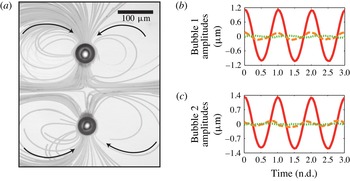
In the case of higher driving frequencies, and as is the case for large bubble radii, an anti-fountain pattern comes out (see figure 5 a). This pattern is the same as the fountain pattern, except that the loops are more elongated perpendicularly to the bubble pair axis and the trajectory orientation is reversed: microbeads are ejected from the bubble pair sides and come back to the bubble along the pair axis. The main modes that appear are still the breathing and the translation modes (see figure 5 b,c). The temporal phase shift between those modes is now positive for each bubble.
(a) Anti-fountain streaming around a bubble pair of radii
 $R_{0}=25~{\rm\mu}\text{m}$
, separated by a distance
 $D=200~{\rm\mu}\text{m}$
and excited at a frequency
 $f_{d}=120~\text{kHz}$
. Black arrows represent the direction of the bead trajectories. (b,c) Amplitude
 $a_{n}(t)$
of the breathing mode (red solid line), the translational mode
 $n=1$
(orange dashed line) and the mode
 $n=2$
(green dotted line), for the two bubbles. The most excited mode is the mode
 $n=1$
and is out of phase with the breathing mode, with
 ${\rm\Delta}{\it\phi}^{(1,0)}={\it\phi}_{1}-{\it\phi}_{0}>0$
for both bubbles and more specifically
 ${\rm\Delta}{\it\phi}_{\#1}^{(1,0)}=+0.1{\rm\pi}$
and
 ${\rm\Delta}{\it\phi}_{\#2}^{(1,0)}=+0.4{\rm\pi}$
. The orientations of mode 1 are respectively
 ${\it\psi}_{1}^{\#1}={\rm\pi}$
for the upper bubble
 $\#1$
and
 ${\it\psi}_{1}^{\#2}=0$
for the lower bubble
 $\#2$
, where the origin is chosen along the
 $x$
-axis. Therefore, the translational mode is responsible of the anti-fountain vortices observed at this frequency.

If the distance between bubbles is identical in both cases with
 $D=200~{\rm\mu}\text{m}$
, in the first case (
 $f_{d}=50~\text{kHz}$
) we expect
 $D$
to be smaller than half a Rayleigh wavelength
 ${\it\lambda}/2\simeq 400~{\rm\mu}\text{m}$
, whereas for the high-frequency case (
 $f_{d}=120~\text{kHz}$
), we expect
 $D$
to be larger than
 ${\it\lambda}/2\simeq 170~{\rm\mu}\text{m}$
. As a result, the average secondary Bjerknes radiation force (Rabaud et al.
Reference Rabaud, Thibault, Mathieu and Marmottant2011) will cause the bubbles to attract each other in the first case and repel each other in the second case, as can be seen on figures 4 and 5 looking at the position of the bubble with respect to the micropits (smaller circles inside the bubbles).
More importantly, this steady attraction or repulsion coincides with the appearance of a mode 1 on each bubble, which oscillates at the same frequency as the driving frequency but with a phase lag with respect to the breathing mode that differs between the two situations. This is most certainly the result of the oscillatory part of the secondary Bjerknes force (see Bjerknes Reference Bjerknes1906; Barbat, Ashgriz & Liu Reference Barbat, Ashgriz and Liu1999; Harkin, Kaper & Nadim Reference Harkin, Kaper and Nadim2001; Rabaud et al.
Reference Rabaud, Thibault, Mathieu and Marmottant2011) exerted from the pulsating neighbouring bubble, and vice versa, which leads to a direct forcing term. As we measured
 ${\it\psi}_{1}^{\#1}={\rm\pi}$
and
 ${\it\psi}_{1}^{\#2}=0$
, the two bubble translations are symmetric: bubbles attract and repel each other by oscillating.
Now, considering the temporal phase
 ${\it\phi}_{n}$
defined in (2.1) for the modes
 $n=0$
and
 $n=1$
, we observe in the case of fountain vortices that each bubble exhibits a negative temporal phase shift between the breathing and translation modes:
 ${\rm\Delta}{\it\phi}^{(1,0)}={\it\phi}_{1}-{\it\phi}_{0}\simeq -{\rm\pi}/5$
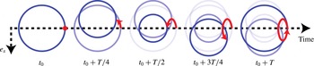
. A non-zero temporal phase shift means that a point located on the liquid/gas interface of the bubble will describe an ellipse. It is illustrated in figure 6 with a sketch showing the bubble movement over an oscillating period when
 ${\rm\Delta}{\it\phi}^{(1,0)}=-{\rm\pi}/2$
. For this value of
 ${\rm\Delta}{\it\phi}^{(1,0)}$
, the elliptical movement of the bubble side has a maximum amplitude. Since the orientation of the elliptical trajectory (red arrow) is determined by the sign of
 ${\rm\Delta}{\it\phi}^{(1,0)}$
, it gives a clue as to why the orientation of the trajectories of figure 5 is reversed for anti-fountain vortices.
This eventually leads to the following interpretation: bubbles are coupled both to the primary field and to the secondary field of the neighbouring bubbles, leading to modes that pulsate synchronously but possibly out of phase. This gives rise to some mixed modes, which, as first introduced by Longuet-Higgins (Reference Longuet-Higgins1997), can enhance the microstreaming. In particular, the mixed mode between breathing (
 $n=0$
) and translation (
 $n=1$
) is typical of a bubble pair and leads to some axial flow symmetry with respect to the bubble axis. Note that parametric modes, if present, would not directly couple with the main breathing mode, since their frequency is
 $f_{d}/2$
and not
 $f_{d}$
.
Schematic representation of the time evolution of a bubble interface during an oscillation period, with a breathing mode and a translation mode in phase quadrature:
 ${\it\phi}_{1}={\it\phi}_{0}-{\rm\pi}/2$
, supposing
 ${\it\Psi}_{1}=0$
.

4 Neighbouring bubbles create a translational mode of the bubble
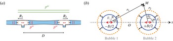
In the following, we propose a theoretical frame to explain the origin of the translation mode in a bubble pair. Considering the Rayleigh wave emission from each bubble of the pair, the total external pressure field experienced by one bubble of the pair is the sum of a primary pressure field
 $p^{ac}$
arising from the piezo-excitation and the pressure field scattered by the neighbouring bubble
 $p^{sc}$
(see figure 7
a). This scattered field can be written:
 $p^{sc}=\text{Re}(\overline{p}^{sc}\text{e}^{\text{i}{\it\omega}_{d}t})$
, where
 $\overline{p}^{sc}=\sum \overline{p}_{n}^{sc}\cos (n{\it\theta}+{\it\psi}_{n}^{sc})$
.
As long as the distance between bubbles is much smaller than the Lamb wavelength in the glass bar,
 $D\ll {\it\lambda}_{glass}$
, we can assume that the primary field is homogeneous, meaning that each bubble of the pair is excited with the same amplitude and the same phase. We also suppose that both bubbles have the same radius
 $R_{0}$
and that the orientation of the modes is fixed by the direction of the bubble pair. We can therefore describe bubble contours following (2.1) and considering the orientation of the mode 1 to be
 ${\it\psi}_{1}^{\#1}={\rm\pi}$
and
 ${\it\psi}_{1}^{\#2}=0$
, where the superscript corresponds to the bubble identification number.
(a) Schematic representation (sectional view) of the deformation of the PDMS walls induced by the bubble pair pulsation, leading to the emission of Rayleigh surface waves. Each bubble generates a scattered field
 $p^{sc}$
that will act as a source for its neighbours. (b) Coordinates and notation for an oscillating bubble pair (top view). We consider two flattened bubbles with the same radius
 $R_{0}$
, located in
 $x_{1}=-D/2$
and
 $x_{2}=+D/2$
. We denote by
 $(r_{1},{\it\theta}_{1})$
and
 $(r_{2},{\it\theta}_{2})$
the polar coordinates in the reference frame of the two bubbles.

We could show in Mekki-Berrada et al. (Reference Mekki-Berrada, Thibault and Marmottant2016) that the response of each mode can be written as a harmonic oscillator response driven by the external field. We obtained a linearized 2D Rayleigh–Plesset equation that incorporates the elasticity of the channel walls (via the Rayleigh wavenumber
 $k$
), linking the bubble vibration modes to the external pressure. For one bubble of the pair we have
 $$\begin{eqnarray}\displaystyle & \displaystyle [-\overline{M}_{0}(R_{0}){\it\omega}_{d}^{2}+K_{0}]\overline{A}_{0}=-\overline{p}^{ac}-\overline{p}_{0}^{sc}, & \displaystyle\end{eqnarray}$$
 $$\begin{eqnarray}\displaystyle & \displaystyle [-\overline{M}_{n}(R_{0}){\it\omega}_{d}^{2}+K_{n}]\overline{A}_{n}=0-\overline{p}_{n}^{sc},\quad \text{for }n\geqslant 1, & \displaystyle\end{eqnarray}$$
 $\overline{M}_{n}(R_{0})$
is the effective mass and
 $K_{n}$
the effective stiffness of the mode
 $n$
. The expressions for these two functions are
 $$\begin{eqnarray}\displaystyle \overline{M}_{n}(r)=-\frac{{\it\rho}_{f}}{k}\frac{\text{H}_{n}^{(2)}(kr)}{\text{H}_{n}^{\prime (2)}(kR_{0})}\quad \text{for }n\geqslant 0,~\forall r\in \mathbb{R}^{+}, & & \displaystyle\end{eqnarray}$$
 $$\begin{eqnarray}\displaystyle K_{0}=\frac{2{\it\gamma}p_{0}}{R_{0}}\quad \text{and}\quad K_{n}=(n-1)(n+1)\frac{{\it\sigma}}{R_{0}^{2}}\quad \text{for }n\geqslant 1, & & \displaystyle\end{eqnarray}$$
where
 $\text{H}_{n}^{(2)}$
denotes the Hankel function of the second kind and of order
 $n$
,
 $\text{H}_{n}^{\prime (2)}$
its derivative (note the following property:
 $\text{H}_{0}^{\prime (2)}=-\text{H}_{1}^{(2)}$
),
 $k$
the Rayleigh wavenumber
 $k={\it\omega}_{d}/c_{R}$
, with
 $c_{R}$
the velocity of the Rayleigh wave at the channel wall interface,
 ${\it\rho}_{f}$
the liquid density,
 ${\it\gamma}$
the adiabatic index,
 $p_{0}$
the static liquid pressure and
 ${\it\sigma}$
the surface tension.
Note that the effective mass
 $\overline{M}_{n}(R_{0})$
is a complex number. Its real part contributes to the natural frequency of the mode
 $n$
,
 $$\begin{eqnarray}\displaystyle {\it\omega}_{n}=\sqrt{\frac{K_{n}}{\text{Re}(\overline{M}_{n}(R_{0}))}}, & & \displaystyle\end{eqnarray}$$
while its imaginary part results in a 2D radiative damping. The expression for the associated damping constant is
 $$\begin{eqnarray}\displaystyle {\it\delta}_{n}^{rad}=-\frac{\text{Im}(\overline{M}_{n}(R_{0}))}{\text{Re}(\overline{M}_{n}(R_{0}))}. & & \displaystyle\end{eqnarray}$$
This 2D radiation damping is related to the emission of Rayleigh waves that are caused by the bubble pulsation. For simplicity, we suppose that this 2D radiation damping dominates the other sources of damping (thermal, viscous, friction at the walls, 3D radiation) in the case of the volume pulsation
 $n=0$
and the translational vibration
 $n=1$
.
To obtain the bubble pair dynamics, we still need to evaluate the scattered pressure field
 $p^{sc}$
. This pressure field is due to the Rayleigh wave scattered by the neighbouring bubble. In the following, we will consider the dynamics of bubble
 $\#1$
.
The axisymmetric pulsation of its neighbour, bubble
 $\#2$
, generates a cylindrical outgoing wave centred on bubble
 $\#2$
. In the reference frame of this bubble (see figure 7
b for the definition of coordinates), the expression for the scattered pressure field in the liquid is
 $$\begin{eqnarray}\displaystyle \overline{p}^{sc}(r_{2},{\it\theta}_{2})=\frac{{\it\rho}_{f}{\it\omega}_{d}^{2}}{k}\frac{\text{H}_{0}^{(2)}(kr_{2})}{\text{H}_{0}^{\prime (2)}(kR_{0})}\overline{A}_{0}^{\,\#2}. & & \displaystyle\end{eqnarray}$$
To express the scattered pressure field in the reference frame
 $(r_{1},{\it\theta}_{1})$
of bubble
 $\#1$
, we write
 $\boldsymbol{r}_{1}=D\boldsymbol{e}_{x}+\boldsymbol{r}_{2}$
, where
 $D$
is the distance between the bubble centres. The scattered field is then calculated on the wall of bubble
 $\#1$
, at
 $r_{1}=R_{0}$
. The expression that we obtain is developed in terms of
 ${\it\epsilon}_{R}=R_{0}/D\ll 1$
. Considering only terms of order less than 1 in
 ${\it\epsilon}_{R}$
we get
 $$\begin{eqnarray}\displaystyle \overline{p}^{sc}(r_{1}=R_{0},{\it\theta}_{1})=\frac{{\it\rho}_{f}{\it\omega}_{d}^{2}}{k}\left[\frac{\text{H}_{0}^{(2)}(kD)}{\text{H}_{0}^{\prime (2)}(kR_{0})}-kD{\it\epsilon}_{R}\frac{\text{H}_{0}^{\prime }(kD)}{\text{H}_{0}^{\prime (2)}(kR_{0})}\cos {\it\theta}_{1}\right]\overline{A}_{0}^{\,\#2}. & & \displaystyle\end{eqnarray}$$
This equation provides the expression for the axisymmetric and monopolar scattered fields,
 $p_{0}^{sc}$
and
 $p_{1}^{sc}$
. The multipolar terms of higher order,
 $p_{n\geqslant 2}^{sc}$
, are negligible compared to those two terms, as they are of order
 $n$
in
 ${\it\epsilon}_{R}$
. Finally, the axisymmetric pulsation of bubble
 $\#2$
behaves like an external excitation source for both the axisymmetric and translational pulsations of bubble
 $\#1$
.
Using the same procedure, we calculate the scattered pressure field generated by bubble
 $\#1$
. We finally get a system of two equations governing the axisymmetric mode dynamics, which can be written in a matrix system as
 $$\begin{eqnarray}\displaystyle \left(\begin{array}{@{}cc@{}}-\overline{M}_{0}(R_{0}){\it\omega}_{d}^{2}+K_{0} & -\overline{M}_{0}(D){\it\omega}_{d}^{2}\\ -\overline{M}_{0}(D){\it\omega}_{d}^{2} & -\overline{M}_{0}(R_{0}){\it\omega}_{d}^{2}+K_{0}\end{array}\right)\left(\begin{array}{@{}c@{}}\overline{A}_{0}^{\,\#1}\\ \overline{A}_{0}^{\,\#2}\end{array}\right)=-\overline{p}^{ac}\boldsymbol{I}_{2}, & & \displaystyle\end{eqnarray}$$
where
 $\boldsymbol{I}_{2}$
is the identity vector. As the two bubbles have the same radius and are identically excited, the breathing mode amplitudes of the two bubbles are equal,
 $\overline{A}_{0}^{\,\#1}=\overline{A}_{0}^{\,\#2}=\overline{A}_{0}$
, and (4.9) leads to
 $$\begin{eqnarray}\displaystyle \overline{A}_{0}=\frac{-\overline{p}^{ac}}{-[\overline{M}_{0}(R_{0})+\overline{M}_{0}(D)]{\it\omega}_{d}^{2}+K_{0}}. & & \displaystyle\end{eqnarray}$$
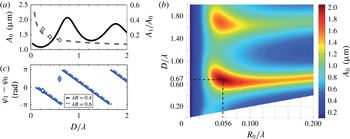
The breathing mode absolute amplitude
 $A_{0}$
has been plotted on figure 8(a) (solid line) for a bubble radius
 $R_{0}=30~{\rm\mu}\text{m}$
and a primary acoustic pressure
 $p^{ac}=14$
kPa. Depending on the distance
 $D$
between the two bubbles, the Rayleigh waves generated by each bubble will interact constructively or destructively, leading respectively to a maximum or a minimum of
 $A_{0}$
.
Origin of the translation mode. (a) Amplitude
 $A_{0}$
of the breathing mode (solid line) and relative amplitude of the translation mode
 $A_{1}/A_{0}$
(dashed line) for a bubble pair of radii
 $R_{0}=30~{\rm\mu}\text{m}$
separated by a distance
 $D$
. The Rayleigh wavelength
 ${\it\lambda}=c_{R}/f_{d}$
is due to the wall deformation when the bubbles are pulsating. It is calculated using
 $c_{R}=40~\text{m}~\text{s}^{-1}$
and at a frequency
 $f_{d}=50~\text{kHz}$
. Secondary resonances appear due to the interaction of the two bubbles via the deformation of the PDMS walls. Experimental data are represented by empty diamonds. (b) Amplitude
 $A_{0}$
of the breathing mode. A maximal value is found for
 $R_{0}/{\it\lambda}=0.056$
and
 $D/{\it\lambda}=0.67$
. (c) Temporal phase shift (in radian) between mode 0 and mode 1 of the same bubble, calculated for two different bubble radii and frequencies:
 $R_{0}=37~{\rm\mu}\text{m}$
and
 $f_{d}=50~\text{kHz}$
, giving
 $kR_{0}=0.4$
(blue, solid line); and
 $R_{0}=25~{\rm\mu}\text{m}$
and
 $f_{d}=120~\text{kHz}$
, giving
 $kR_{0}=0.6$
(cyan, dashed line), when they are separated by a distance
 $D$
. Experimental data are represented by diamonds. The translation mode of both bubbles is in phase, showing that bubbles successively attract and repel each other.

By changing the two bubbles’ radii, we draw a map of the breathing mode absolute amplitude
 $A_{0}$
with the two varying parameters
 $R_{0}/{\it\lambda}$
and
 $D/{\it\lambda}$
, where
 ${\it\lambda}$
is the wavelength of the Rayleigh wave in the PDMS wall and is calculated using
 $c_{R}=40~\text{m}~\text{s}^{-1}$
(see figure 8
b). In the case of an isolated bubble,
 $D$
tends to infinity and (4.10) leads to a pulsation resonance in
 $R_{0}/{\it\lambda}=0.049$
. For a bubble pair, a first maximum is obtained for an inter-bubble distance
 $D^{res}=0.67{\it\lambda}$
and a bubble radius
 $R_{0}=0.056{\it\lambda}$
. Secondary maxima appear when
 $D=N{\it\lambda}+D^{res}$
, with
 $N$
an integer.
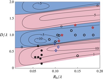
Conditions for the existence of fountain and anti-fountain long-range streaming patterns as a function of the reduced radii
 $R_{0}/{\it\lambda}$
and bubble-to-bubble distance
 $D/{\it\lambda}$
. Filled (empty) symbols correspond to experiments with fountain (anti-fountain) vortices. Star symbols correspond to bubbles excited above the threshold of the parametric instability. Blue diamonds correspond to quadrupolar patterns observed on each bubble of a pair. The lines correspond to isovalues (
 $\text{mm}~\text{s}^{-1}$
) of the maximal streaming velocity for a combination of modes 0 and 1 at different bubble radii and inter-bubble distances (non-dimensionalized with the Rayleigh wavelength
 ${\it\lambda}$
). Light red (dark blue) regions correspond to the predicted fountain (anti-fountain) regions for the driving pressure
 $P_{ac}=14~\text{kPa}$
and a fitted sound velocity
 $c_{R}$
of
 $30~\text{m}~\text{s}^{-1}$
. (See § 5 for a discussion.)

We can now write the equations governing the translation mode of the two bubbles:
 $$\begin{eqnarray}\displaystyle & \displaystyle -\overline{M}_{1}(R_{0}){\it\omega}_{d}^{2}\overline{A}_{1}^{\,\#1}=kR_{0}\overline{M}_{0}^{\prime }(D){\it\omega}_{d}^{2}\overline{A}_{0}^{\,\#2}, & \displaystyle\end{eqnarray}$$
 $$\begin{eqnarray}\displaystyle & \displaystyle -\overline{M}_{1}(R_{0}){\it\omega}_{d}^{2}\overline{A}_{1}^{\,\#2}=kR_{0}\overline{M}_{0}^{\prime }(D){\it\omega}_{d}^{2}\overline{A}_{0}^{\,\#1}. & \displaystyle\end{eqnarray}$$
 ${\it\psi}_{1}^{sc}={\rm\pi}$
for bubble
 $\#1$
. Finally, we obtain
 $\overline{A}_{1}^{\,\#1}=\overline{A}_{1}^{\,\#2}=\overline{A}_{1}$
, with
 $$\begin{eqnarray}\displaystyle \overline{A}_{1}=-kR_{0}\frac{\overline{M}_{0}^{\prime }(D)}{\overline{M}_{1}(R_{0})}\overline{A}_{0}. & & \displaystyle\end{eqnarray}$$
The relative amplitude
 $A_{1}/A_{0}$
of the translation mode compared to the breathing mode has been plotted on figure 8(a) (dashed line) for a bubble radius
 $R_{0}=30~{\rm\mu}\text{m}$
and a primary acoustic pressure
 $p^{ac}=14~\text{kPa}$
. We find that
 $A_{1}/A_{0}$
decreases with the distance between bubbles, since it is proportional to
 $\text{H}_{1}^{(2)}(kD)$
, which tends to zero by oscillating when bubbles move away from each other:
 $$\begin{eqnarray}\displaystyle \lim _{kD\rightarrow \infty }\text{H}_{1}^{(2)}(kD)=\sqrt{\frac{2}{{\rm\pi}kD}}\,\text{e}^{-\text{i}(kD-3{\rm\pi}/4)}. & & \displaystyle\end{eqnarray}$$
In fact, the further the bubbles are from each other, the less they feel the Rayleigh wave generated by the others. We also reported on figure 8 the measurements of
 $A_{1}/A_{0}$
for the experiments shown on figures 4 and 5. They show a good agreement with the model. Equation (4.13) also gives access to the phase shift
 ${\rm\Delta}{\it\phi}^{(1,0)}={\it\phi}_{1}-{\it\phi}_{0}$
between the breathing and translation modes. Figure 8(c) reports the evolution of this phase shift with the distance
 $D$
between bubbles for two different values of
 $kR_{0}$
that correspond to the two experimental conditions of figures 4 and 5. We notice that the two bubbles have the same phase shift, meaning that their translational motion is symmetrical to the median plane of the pair. Moreover, we find that
 ${\rm\Delta}{\it\phi}^{(1,0)}$
changes regularly in sign when the distance
 $D$
is increasing. The critical distances for which the phase shift changes its sign are only slightly affected by an increase of the bubble radius (see the solid and dashed lines). The phase shift measurements are reported on the figure for the two cases described in figures 4 and 5. They agree nicely with the model in the case of a fountain streaming pattern but we notice a shift in the case of anti-fountain streaming patterns.
Using the reduced parameters
 $R_{0}/{\it\lambda}$
and
 $D/{\it\lambda}$
, we gathered on figure 9 the experimental conditions (see the symbols) for the different types of streaming that we obtained by varying the bubble radii, the inter-bubble distance and the driving frequency. In particular, fountain vortices have been observed for values of
 $R_{0}/{\it\lambda}<0.1$
and anti-fountain vortices for larger values of
 $R_{0}/{\it\lambda}$
, whereas the distance between bubbles must be kept small (
 $D/{\it\lambda}<1$
) to favour interactions between neighbouring bubbles. In the limit of bubbles that have been brought into contact (
 $D=2R_{0}$
), the same observations hold. In addition, we distinguished experimental data with bubbles excited below (circles and diamonds on figure 9) and above (red stars) the threshold of the parametric instability. In both cases, we can observe long-range fountain or anti-fountain vortices, which are not related to the presence of surface modes. Therefore, if surface modes contribute to streaming, their influence is restricted to short distances, as suggested by figure 2(a).
Last, a Fourier series analysis shows that, in some conditions, the amplitude
 $A_{2}$
of the quadrupolar mode is no longer negligible compared to the breathing and translation modes (see § A.1). With this new mode, a new streaming pattern is observed, consisting of two large vortices and two small vortices around each bubble (blue diamonds on figure 9). The two small vortices are located in between the two bubbles.
5 Mixed-mode streaming theory including bubble interaction
Knowing the amplitude of the bubble vibrations and their phase shift, we now develop a theory following the approach of Longuet-Higgins (Reference Longuet-Higgins1998) for the 3D streaming around a spherical bubble and of Rallabandi et al. (Reference Rallabandi, Wang and Hilgenfeldt2014) for the 2D streaming around a semi-cylindrical bubble attached to a wall.
In the following, we consider the streaming generated by the vibration of one single flattened bubble. The streaming flow is assumed to be incompressible. The 2D velocity field is described by a streamfunction
 ${\it\Psi}$
related to the velocity components in polar coordinates,
 $u_{r}=(1/r)\partial _{{\it\theta}}{\it\Psi}$
and
 $u_{{\it\theta}}=-\partial _{r}{\it\Psi}$
, where
 $r$
and
 ${\it\theta}$
are the polar coordinates in the frame associated with the centre of the bubble. Later on, we will distinguish the two bubbles by replacing
 $r$
by
 $r_{j}$
and
 ${\it\theta}$
by
 ${\it\theta}_{j}$
for the bubble
 $\#j$
(with
 $j=1,2$
).
For small oscillations of the mode
 $k$
, of relative amplitude
 ${\it\epsilon}_{k}\sim A_{k}/R_{0}\ll 1$
, we develop the Navier–Stokes solution in ascending orders of
 ${\it\epsilon}_{k}$
. Up to the second order we have
 $$\begin{eqnarray}\displaystyle {\it\Psi}=\mathop{\sum }_{k}{\it\epsilon}_{k}{\it\Psi}_{1}^{(k)}+\mathop{\sum }_{m,n}{\it\epsilon}_{m}{\it\epsilon}_{n}{\it\Psi}_{2}^{(m,n)}+o({\it\epsilon}_{k}^{2}), & & \displaystyle\end{eqnarray}$$
where
 ${\it\Psi}_{1}^{(k)}$
is the linear oscillating solution and
 ${\it\Psi}_{2}^{(m,n)}$
the nonlinear part with a non-zero continuous part
 $\langle {\it\Psi}_{2}^{(m,n)}\rangle$
that thus contributes to the steady streaming.
The first-order
 ${\it\Psi}_{1}^{(k)}$
satisfies the vorticity equation,
 $$\begin{eqnarray}\displaystyle \frac{\partial {\rm\Delta}{\it\Psi}_{1}^{(k)}}{\partial t}={\it\nu}{\rm\Delta}^{2}{\it\Psi}_{1}^{(k)}, & & \displaystyle\end{eqnarray}$$
where
 ${\rm\Delta}$
is the Laplace operator.
The boundary conditions at the bubble interface are the continuity of the normal velocity and a vanishing tangential component of the stress:
 $$\begin{eqnarray}\displaystyle \left.\begin{array}{@{}c@{}}\displaystyle \frac{1}{r}\partial _{{\it\theta}}{\it\Psi}_{1}^{(k)}=R_{0}{\it\omega}_{d}\cos (k{\it\theta})\text{e}^{\text{i}{\it\omega}_{d}t},\\ \displaystyle \partial _{r}^{2}{\it\Psi}_{1}^{(k)}-\frac{1}{r}\partial _{r}{\it\Psi}_{1}^{(k)}-\frac{1}{r^{2}}\partial _{{\it\theta}}^{2}{\it\Psi}_{1}^{(k)}=0,\end{array}\right\}\quad \text{on }r=R_{0}. & & \displaystyle\end{eqnarray}$$
Note that the assumption of free slip may not be appropriate. In fact, it was observed in some cases that the surfactant could form a flexible skin at the bubble interface (Elder Reference Elder1958). In that case, no-slip boundary conditions should be considered, corresponding to the continuity of both normal and tangential velocities:
 $$\begin{eqnarray}\displaystyle \left.\begin{array}{@{}c@{}}\displaystyle \frac{1}{r}\partial _{{\it\theta}}{\it\Psi}_{1}^{(k)}=R_{0}{\it\omega}_{d}\cos (k{\it\theta})\text{e}^{\text{i}{\it\omega}_{d}t},\\ \displaystyle -\partial _{r}{\it\Psi}_{1}^{(k)}=0,\end{array}\right\}\quad \text{on }r=R_{0}. & & \displaystyle\end{eqnarray}$$
Depending on the concentration of surfactant, we might be closer to one case or the other. In both cases, we look for a solution
 ${\it\Psi}_{1}^{(k)}\propto R_{0}^{2}{\it\omega}_{d}\sin (k{\it\theta})\text{e}^{\text{i}{\it\omega}_{d}t}$
. The vorticity equation can also be written as
 $$\begin{eqnarray}\displaystyle ({\rm\nabla}^{2}-{\it\alpha}^{2}){\rm\nabla}^{2}{\it\Psi}_{1}^{(k)}=0, & & \displaystyle\end{eqnarray}$$
where
 ${\it\alpha}=(1+\text{i})/{\it\delta}$
and
 ${\it\delta}=\sqrt{2{\it\nu}/{\it\omega}_{d}}$
is the thickness of the oscillatory ‘Stokes layer’. The modified Bessel equation
 $({\rm\nabla}^{2}-{\it\alpha}^{2}){\it\Psi}_{1}^{(k)}=0$
has the following solutions: the exponentially increasing solution
 $I_{k}({\it\alpha}r)$
and the exponentially decreasing solution
 $\text{K}_{k}({\it\alpha}r)$
. As
 ${\it\Psi}_{1}^{(k)}$
should tend to zero at long distance, only the modified Bessel solution of the second kind
 $\text{K}_{k}({\it\alpha}r)$
remains. Laplace’s equation
 ${\rm\nabla}^{2}{\it\Psi}_{1}^{(k)}=0$
can be solved using the separation of variables method, leading to solutions in
 $1/r^{k}$
. Finally, we have
 $$\begin{eqnarray}\displaystyle {\it\Psi}_{1}^{(k)}=R_{0}^{2}{\it\omega}_{d}\left(\frac{c_{k}}{r^{k}}+d_{k}\text{K}_{k}({\it\alpha}r)\right)\sin (k{\it\theta})\text{e}^{\text{i}{\it\omega}_{d}t}. & & \displaystyle\end{eqnarray}$$
Using the two boundary conditions, we finally get the values of the constants:
 $$\begin{eqnarray}\displaystyle c_{k}=R_{0}^{k}\left(\frac{1}{k}-d_{k}\text{K}_{k}({\it\alpha}R_{0})\right) & & \displaystyle\end{eqnarray}$$
and
 $$\begin{eqnarray}\displaystyle \left.\begin{array}{@{}ll@{}}\displaystyle d_{k}=\frac{2(k+1)}{({\it\alpha}R_{0})^{2}K_{k-2}({\it\alpha}R_{0})-2k{\it\alpha}R_{0}K_{k-1}({\it\alpha}R_{0})} & \text{for slip boundary conditions},\\ \displaystyle d_{k}=\frac{1}{{\it\alpha}R_{0}K_{k-1}({\it\alpha}R_{0})} & \text{for no-slip boundary conditions}.\end{array}\right\} & & \displaystyle \nonumber\\ \displaystyle & & \displaystyle\end{eqnarray}$$
In the following, we will consider only the case of a free slip at the bubble interface. The continuous (time-average) part of the second-order terms also satisfies the vorticity equation, which reduces in this case to
 $$\begin{eqnarray}\displaystyle {\rm\Delta}^{2}\langle {\it\Psi}_{2}^{(m,n)}\rangle =-\frac{1}{{\it\nu}}\left\langle \frac{1}{r}\frac{\partial ({\it\Psi}_{1}^{(m)},{\rm\Delta}{\it\Psi}_{1}^{(n)})}{\partial (r,{\it\theta})}\right\rangle , & & \displaystyle\end{eqnarray}$$
where
 $(\partial (f,g)/\partial (r,{\it\theta}))$
is the Jacobian determinant and
 $\langle ~\rangle$
denotes the time average. The right-hand term of (5.9) derives from the Reynolds stress, which is defined as the mean value of the acoustic momentum flux and is known to force the acoustic streaming (Lighthill Reference Lighthill1978). We now introduce
 ${\it\eta}=(r-R_{0})/{\it\delta}$
as in Longuet-Higgins (Reference Longuet-Higgins1998). As
 ${\it\delta}\ll R_{0}$
, we can use the asymptotic form of
 $\text{K}_{k}$
and its derivatives. The detailed calculation is proposed in Rallabandi et al. (Reference Rallabandi, Wang and Hilgenfeldt2014) and shows that (5.9) gives rise to particular solutions that are proportional to
 $({\it\delta}/R_{0})^{2}\text{e}^{-(1+\text{i}){\it\eta}}$
. Thus, the only solutions of order zero in
 ${\it\delta}/R_{0}$
are the homogeneous solutions of the biharmonic equation. They are called Michell solutions, and if we only keep terms that decrease with the distance, we get
 $$\begin{eqnarray}\displaystyle \langle {\it\Psi}_{2}\rangle =\mathop{\sum }_{k=1}^{\infty }\frac{e_{k}}{r^{k}}\sin (k{\it\theta})+\mathop{\sum }_{k=3}^{\infty }\frac{f_{k}}{r^{k-2}}\sin (k{\it\theta}), & & \displaystyle\end{eqnarray}$$
with
 $e_{k}$
and
 $f_{k}$
constants to determine.
One should add the Stokes drift component
 ${\it\Psi}_{d}$
to get the Lagrangian streamfunction describing the motion of particles:
 $$\begin{eqnarray}\displaystyle {\it\Psi}_{L}=\mathop{\sum }_{m,n}{\it\epsilon}_{m}{\it\epsilon}_{n}(\langle {\it\Psi}_{2}^{(m,n)}\rangle +{\it\Psi}_{d}^{(m,n)}). & & \displaystyle\end{eqnarray}$$
The Stokes drift satisfies the following equation (Raney, Corelli & Westervelt Reference Raney, Corelli and Westervelt1954):
 $$\begin{eqnarray}\displaystyle {\it\Psi}_{d}^{(m,n)}=\left\langle \frac{1}{r}\partial _{{\it\theta}}{\it\Psi}_{1}^{(m)}\int (-\partial _{r}{\it\Psi}_{1}^{(n)})\,\text{d}t\right\rangle +\left\langle \frac{1}{r}\partial _{{\it\theta}}{\it\Psi}_{1}^{(n)}\int (-\partial _{r}{\it\Psi}_{1}^{(m)})\,\text{d}t\right\rangle . & & \displaystyle\end{eqnarray}$$
Using (5.8), and considering only terms of order zero in
 ${\it\delta}$
, we finally get
 $$\begin{eqnarray}\displaystyle {\it\Psi}_{d}^{(m,n)}=\frac{1}{2}R_{0}^{2}{\it\omega}_{d}\left(\frac{R_{0}}{r}\right)^{m+n+2}\sin ({\it\phi}_{m}-{\it\phi}_{n})\sin ((m-n){\it\theta}). & & \displaystyle\end{eqnarray}$$
The Lagrangian streamfunction must satisfy the following boundary condition at the bubble interface:
 $$\begin{eqnarray}\displaystyle \frac{1}{r}\partial _{{\it\theta}}{\it\Psi}_{L}=0\quad \text{on }r=R_{0}. & & \displaystyle\end{eqnarray}$$
This last equation allows us to set the coefficients
 $e_{k}$
and
 $f_{k}$
of the Michell solutions for the streaming
 $\langle {\it\Psi}_{2}\rangle$
in (5.10), and to obtain the Lagrangian streamfunction.
We evaluate this streamfunction (keeping only terms of order zero in
 ${\it\delta}/R_{0}$
) for two sets of mixed modes, as follows.
-
(i) When the bubble exhibits a mode
 $m=0$
and a mode
$n=1$
, we get (5.15)The decay of the streamfunction at long distances is thus weak, scaling in
$$\begin{eqnarray}\displaystyle {\it\Psi}_{L}=\frac{1}{2}A_{1}A_{0}{\it\omega}_{d}\left[\left(\frac{R_{0}}{r}\right)^{3}-\frac{R_{0}}{r}\right]\sin ({\it\phi}_{1}-{\it\phi}_{0})\sin ({\it\theta}). & & \displaystyle\end{eqnarray}$$
$r^{-1}$
, meaning that velocities decrease as
$r^{-2}$
.
-
(ii) When the bubble exhibits a mode
$m=0$
, a mode
$n=1$
and a mode
$n^{\prime }=2$
, we get (5.16)
$$\begin{eqnarray}\displaystyle {\it\Psi}_{L} & = & \displaystyle \frac{1}{2}A_{1}A_{0}{\it\omega}_{d}\left[\left(\frac{R_{0}}{r}\right)^{3}-\frac{R_{0}}{r}\right]\sin ({\it\phi}_{1}-{\it\phi}_{0})\sin ({\it\theta})+O\left(\frac{1}{r^{5}}\right)\nonumber\\ \displaystyle & & \displaystyle +\,\frac{1}{2}A_{2}A_{0}{\it\omega}_{d}\left[\left(\frac{R_{0}}{r}\right)^{4}-\left(\frac{R_{0}}{r}\right)^{2}\right]\sin ({\it\phi}_{2}-{\it\phi}_{0})\sin (2{\it\theta}).\end{eqnarray}$$


According to these equations, one can now obtain the amplitude of the streaming velocities. Deriving (5.15) gives for the maximum velocity at the bubble interface:
 $$\begin{eqnarray}\displaystyle V_{max}=\frac{A_{0}A_{1}}{R_{0}}{\it\omega}_{d}\sin ({\it\phi}_{1}-{\it\phi}_{0}). & & \displaystyle\end{eqnarray}$$
Now, depending on the sign of
 ${\it\phi}_{1}-{\it\phi}_{0}$
, the prefactor of the streamfunction
 ${\it\Psi}_{L}$
will be either negative for the bubble located in
 $x=+D/2$
, leading to fountain vortices, or positive, leading to anti-fountain vortices. The full phase diagram is represented on figure 9, where we show the isovalues of the maximal streaming velocity as a function of the reduced radii
 $R_{0}/{\it\lambda}$
and bubble-to-bubble distance
 $D/{\it\lambda}$
. The plot corresponds to a driving pressure
 $p^{ac}=14~\text{kPa}$
, and a sound velocity
 $c_{R}$
of
 $30~\text{m}~\text{s}^{-1}$
, leading to streaming velocities up to
 $10~\text{mm}~\text{s}^{-1}$
. The theory and the experiments are in good agreement for the explored experimental range of bubbles and distances.
6 Detailed study of a fountain pattern: comparison between theory and experiment
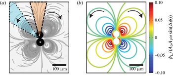
Since the previous model gives an explicit solution for the whole flow field, we are now in a position for a direct comparison with the experiments. We thus consider the situation of figure 10(a) of two bubbles in close contact, with the external flow field materialized by using stack images of the positions of microbeads seeding the flow.
(a) Streaming pattern around a bubble pair in contact. We consider two angular sectors respectively centred around
 ${\it\Theta}=0$
(dashed delimited orange sector) and
 ${\it\Theta}={\rm\pi}/4$
(dotted delimited cyan sector). The origin of the sector is the middle in between the bubble centres. (b) Simulation of the streamlines around a bubble pair in contact (
 $D=2R_{0}$
) exhibiting a breathing and a translation mode. We assume here the additivity of the streamfunctions of the bubbles. Black arrows show the predicted direction of the flow in the case of a negative
 ${\rm\Delta}{\it\phi}$
.

To compare these experimental data with the theory, we have plotted on figure 10(b) the simulated flow pattern. For this, we considered that, for each single bubble, the mixed mode between modes 0 and 1 is dominant and is described by (5.15). Then, we assumed that the total stream field is the superposition of the two fields obtained for each bubble, i.e.
 $~{\it\psi}_{L}={\it\psi}_{L}^{\#1}+{\it\psi}_{L}^{\#2}$
, and that the two bubbles are separated by a distance
 $D=2R_{0}$
and vibrate identically. From a simple visual comparison, we see that the theory captures the major trends of the long-range microstreaming, with the presence of a global quadrupole oriented along the bubble axis. This experiment validates the assumption of the additivity of streamfunctions away from the bubble pair, even when the two bubbles are stuck to each other, and goes in the direction of a mixed-mode streaming with modes 0 and 1. However, if the similarity between experimental and theoretical patterns is indicative of the flow symmetries, we still need to measure the velocity magnitude all around the bubble pair to test the validity of the mixed-mode model.
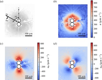
Velocity field obtained by performing PTV on the experiment of figure 10(a). (a) Velocity field and reference frame for the radial and tangential velocities
 $u_{R}$
and
 $u_{{\it\Theta}}$
, (b) modulus of the local velocity, (c) value of the radial component of the velocity, and (d) value of the tangential component of the velocity. Radial and tangential components are extracted, taking a frame with origin at the centre of mass of the two bubbles. Raw data obtained from PTV are filtered using a gradient filter and interpolated using an inverse direct weighting interpolation.

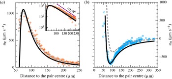
Experimental data for (a)
 $u_{R}$
and (b)
 $u_{{\it\Theta}}$
respectively plotted for the orange (dashed delimited) and cyan (dotted delimited) zones of figure 10(a). Inset: logarithmic representation of (a). Reference for the distances are taken at the contact point of the bubbles (see figure 10). Non-filtered data are used in order to increase the dynamics of the plot. Two models are also presented: velocity prediction for two bubbles exhibiting a mode 0 and a mode 1 (solid line) derived from (A 1)–(A 2), and velocity prediction for a single bubble exhibiting a mode 0 and a mode 2 (dashed line) derived from (A 7) and (A 8). Supposing that the two bubbles behave identically, the fitting curve gives access to the value
 $A_{0}A_{1}\sin ({\rm\Delta}{\it\phi})=-0.74~{\rm\mu}\text{m}^{2}$
for each bubble and a theoretical radius of
 $30~{\rm\mu}\text{m}$
. For the empirical one-bubble model, curve fitting leads to an equivalent radius of
 $55~{\rm\mu}\text{m}$
and
 $A_{0}A_{2}\sin ({\rm\Delta}{\it\phi})=-1.24~{\rm\mu}\text{m}^{2}$
.

The full velocity field is initially obtained from PTV (figure 11
a) and reconstructed in the channel plane, according to the interpolation scheme discussed in § 2.2. Then, taking a frame with origin at the centre of mass of the two bubbles and oriented along their centre, we introduce new polar coordinates
 $(R;{\it\Theta})$
. In this frame, the radial and tangential components
 $u_{R}$
and
 $u_{{\it\Theta}}$
are extracted (figure 11
c,d), whereas the total velocity magnitude is reported on figure 11(b).
To go into a quantitative description, we now derive from (5.15) the components of the velocity field for each bubble
 $\#j$
(with
 $j$
being 1 or 2), in the frame of the bubble centre:
 $$\begin{eqnarray}\displaystyle & \displaystyle u_{r}^{\#j}=\frac{1}{2}\frac{A_{1}A_{0}}{r_{j}}{\it\omega}_{d}\left[-\frac{R_{0}}{r_{j}}+\left(\frac{R_{0}}{r_{j}}\right)^{3}\right]\sin ({\it\phi}_{1}-{\it\phi}_{0})\cos ({\it\theta}_{j}), & \displaystyle\end{eqnarray}$$
 $$\begin{eqnarray}\displaystyle & \displaystyle u_{{\it\theta}}^{\#j}=\frac{1}{2}\frac{A_{1}A_{0}}{R_{0}}{\it\omega}_{d}\left[-\left(\frac{R_{0}}{r_{j}}\right)^{2}+3\left(\frac{R_{0}}{r_{j}}\right)^{4}\right]\sin ({\it\phi}_{1}-{\it\phi}_{0})\sin ({\it\theta}_{j}). & \displaystyle\end{eqnarray}$$
 $u_{R}$
and
 $u_{{\it\Theta}}$
, with the origin taken at the mid-point between the two bubbles, are given in § A.2.
Since both
 $u_{R}$
and
 $u_{{\it\Theta}}$
are functions of
 $R$
and
 ${\it\Theta}$
, and since the model clearly captured the
 ${\it\Theta}$
dependence, we now consider only two angular sectors respectively centred around
 ${\it\Theta}=0$
and
 ${\it\Theta}={\rm\pi}/4$
(see figure 10
a) to discuss the radial dependence. Owing to the flow symmetries, we have for these particular angles
 $u_{{\it\Theta}}(R,0)=0$
and
 $u_{R}(R,{\rm\pi}/4)=0$
, leading to a direct determination of the radial dependence of
 $u_{R}$
and
 $u_{{\it\Theta}}$
. The results, averaged over the angular sector, are represented on figure 12(a,b) and are compared to the best fit based on a mixed mode between 0 and 1 according to (A 1)–(A 2), assuming that both bubbles have the same vibration amplitudes. The agreement is excellent with the theory developed in § 5, except maybe for the highest values of
 $R$
. Experimentally, the radial velocity is found to decrease in
 $R^{-3}$
in the far-field region around the bubble pair, which corresponds to the prediction given by the mixed-mode model (see (A 5) in appendix A). In comparison, the mixed-mode streaming induced by a pair of spherical bubbles (see Longuet-Higgins Reference Longuet-Higgins1998) would lead to a radial velocity decreasing in
 $R^{-2}$
. Again, the maximum of the velocity
 $V_{max}\approx 950~{\rm\mu}\text{m}~\text{s}^{-1}$
gives an idea of the streaming velocity that can be generated from two interacting bubbles.
For exhaustiveness, we also compared these measurements with an empirical model in which we consider the streaming flow of a single bubble of radius
 $2R_{0}$
located at the centre of the two bubbles and showing a mixed mode between a mode 0 and 2, as described in § A.3 by (A 7) and (A 8). The result, superimposed on the experimental data, also provides a very good fit especially far away from the bubbles. This was indeed expected since such a mode is quadrupolar in nature and since two bubbles in close contact have strongly coupled pulsations and can be seen as a single pulsating object.
7 Conclusions
We have shown that two freely pulsating bubbles in a confined geometry can generate intense streaming, which results from a unique combination of large vibration amplitudes of individual bubbles and additional higher-order modes resulting from bubble interaction through surface waves in the microfluidic channel. We have developed a theory of mixed-mode streaming for two interacting confined bubbles. The streaming velocities are found to be proportional to the amplitude of the modes that are excited, and also to the sine of the relative phase of the two modes that are involved. In the case of the semi-cylindrical bubbles studied by Wang et al. (Reference Wang, Rallabandi and Hilgenfeldt2013), bubbles are anchored to the channel side wall, which allows the appearance of non-parametric shape modes that can interact with each other. For freely oscillating cylindrical bubbles, shape modes are parametric and thus oscillate at
 ${\it\omega}_{n}={\it\omega}_{d}/2$
. As two successive parametric shape modes cannot appear at the same time, they do not produce long-range streaming. However, as the contour of the cylindrical bubble is not anchored, shape modes can rotate, leading to more complex trajectories close to the bubble wall. The use of these rotating modes could lead to more efficient mixing around the bubbles. As a perspective one can imagine a generalization of the previous mechanism to study the collective properties of a large number of interacting bubbles, and its application to mixing for instance. This approach is currently under progress.
Acknowledgements
The research leading to these results has received funding from Region Rhône-Alpes and the European Research Council under the European Community’s Seventh Framework Programme (FP7/2007-2013) ERC Grant Agreement Bubbleboost no. 614655.
Appendix A
A.1 Higher-order modes flow patterns
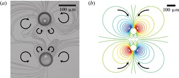
Eventually, we can tackle more complex flow patterns, as illustrated by figure 13, which shows two bubbles of large radii
 $R_{0}=38~{\rm\mu}\text{m}$
separated by
 $200~{\rm\mu}\text{m}$
and excited with a primary field at high frequency
 $f_{d}=120~\text{kHz}$
. Whereas anti-fountain vortices are clearly visible on both sides of the bubble pairs, two pairs of smaller vortices are also observed between the bubbles. This is a clear evidence of the presence of both mixed modes combining modes 0 and 1 and modes 0 and 2, with a reduced amplitude of the mixed mode (0, 2) since the amplitudes of the modes decay with the mode number
 $n$
. In the current case, the vibration mode analysis allows us to determine for both bubbles the amplitude of the most dominant modes,
 $A_{0}=2~{\rm\mu}\text{m}$
,
 $A_{1}=0.3~{\rm\mu}\text{m}$
and
 $A_{2}=0.1~{\rm\mu}\text{m}$
, and their temporal phase shifts,
 ${\rm\Delta}{\it\phi}^{(0,1)}=+0.3$
rad and
 ${\rm\Delta}{\it\phi}^{(0,2)}=+1.9$
rad. Using (5.16) and assuming that the global streamfunction is given by
 ${\it\Psi}_{L}={\it\Psi}_{L}^{\#1}+{\it\Psi}_{L}^{\#2}$
, we can draw the streamlines around the bubble pair by using the experimental parameters (see figure 13
b). We obtain a very satisfactory agreement between experimental and simulated patterns. The conditions for the appearance of this pattern still need to be investigated. These patterns appear for large bubbles separated by a distance of approximately half the Rayleigh wavelength (see the blue diamonds on figure 9). As we can see in figure 13(a), the two bubbles repel each other strongly. Therefore, the micropits might play a role in the generation of this quadrupolar streaming pattern.
Interaction between the monopole and quadrupole modes for a bubble pair of radius
 $R_{0}=38~{\rm\mu}\text{m}$
separated by a distance
 $D=200~{\rm\mu}\text{m}$
and excited at a frequency
 $f_{d}=120~\text{kHz}$
. (a) Experimental pattern observed around the bubble pair. Black arrows represent the direction of the bead trajectories. Small vortices appear between the two bubbles. (b) Simulation of the streamlines around a bubble pair exhibiting a breathing, a translation and a quadrupolar mode for the same conditions, with the mode amplitudes
 $A_{0}=2~{\rm\mu}\text{m}$
,
 $A_{1}=0.3~{\rm\mu}\text{m}$
and
 $A_{2}=0.1~{\rm\mu}\text{m}$
and temporal phase shifts
 ${\rm\Delta}{\it\phi}^{(0,1)}=+0.3~\text{rad}$
and
 ${\rm\Delta}{\it\phi}^{(0,2)}=+1.9~\text{rad}$
.

A.2 Velocity field due to two bubbles exhibiting a mode 0 and a mode 1
Assuming that the streamfunctions for a bunch of bubbles are additive, we can calculate the velocity field produced by two bubbles by saying
 ${\it\Psi}_{L}={\it\Psi}_{L}^{\#1}+{\it\Psi}_{L}^{\#2}$
. The expressions for the radial and tangential velocities in the frame of the bubble pair centre are
 $$\begin{eqnarray}\displaystyle u_{R} & = & \displaystyle \displaystyle -{\it\alpha}_{1}\frac{R_{0}}{r_{1}^{4}}\left\{\frac{RD}{r_{1}^{2}}(2R_{0}^{2}-r_{1}^{2})\sin ^{2}{\it\Theta}+(R_{0}^{2}-r_{1}^{2})\cos {\it\Theta}\right\}\nonumber\\ \displaystyle & & \displaystyle +\,\displaystyle {\it\alpha}_{2}\frac{R_{0}}{r_{2}^{4}}\left\{-\frac{RD}{r_{2}^{2}}(2R_{0}^{2}-r_{2}^{2})\sin ^{2}{\it\Theta}+(R_{0}^{2}-r_{2}^{2})\cos {\it\Theta}\right\}\end{eqnarray}$$
 $$\begin{eqnarray}\displaystyle u_{{\it\Theta}} & = & \displaystyle \displaystyle -{\it\alpha}_{1}\frac{R_{0}}{r_{1}^{4}}\left\{\frac{R}{r_{1}^{2}}(2R+D\cos {\it\Theta})(2R_{0}^{2}-r_{1}^{2})-(R_{0}^{2}-r_{1}^{2})\right\}\sin {\it\Theta}\nonumber\\ \displaystyle & & \displaystyle +\,\displaystyle {\it\alpha}_{2}\frac{R_{0}}{r_{2}^{4}}\left\{\frac{R}{r_{2}^{2}}(2R-D\cos {\it\Theta})(2R_{0}^{2}-r_{2}^{2})-(R_{0}^{2}-r_{2}^{2})\right\}\sin {\it\Theta},\end{eqnarray}$$
 $r_{j}$
is the distance to the centre of bubble
 $\#j$
(
 $j=1,2$
),
 $$\begin{eqnarray}\displaystyle r_{j}=\sqrt{R^{2}+\frac{D^{2}}{4}+{\it\delta}_{j}RD\cos {\it\Theta}}\quad \text{with }\left.\begin{array}{@{}c@{}}{\it\delta}_{1}=+1,\\ {\it\delta}_{2}=-1,\end{array}\right\} & & \displaystyle\end{eqnarray}$$
and
 ${\it\alpha}_{j}$
is the streaming prefactor of bubble
 $\#j$
(
 $j=1,2$
),
 $$\begin{eqnarray}\displaystyle {\it\alpha}_{j}={\textstyle \frac{1}{2}}A_{0}^{\#j}A_{1}^{\#j}{\it\omega}_{d}\sin {\rm\Delta}{\it\phi}^{\#j}. & & \displaystyle\end{eqnarray}$$
In the particular case of two bubbles having the same amplitude and phase of vibration
 ${\it\alpha}={\it\alpha}_{1}={\it\alpha}_{2}$
, we can develop (A 1)–(A 2) in Taylor series far away from the bubble pair (
 $R\gg D$
). We get at first order
 $$\begin{eqnarray}\displaystyle & \displaystyle u_{R}={\it\alpha}\left(-\frac{2DR_{0}}{R^{3}}+\frac{DR_{0}(4R_{0}^{2}+D^{2})}{R^{5}}+o\left(\frac{1}{R^{5}}\right)\right)\cos 2{\it\Theta}, & \displaystyle\end{eqnarray}$$
 $$\begin{eqnarray}\displaystyle & \displaystyle u_{{\it\Theta}}={\it\alpha}\left(-\frac{2DR_{0}}{R^{3}}+\frac{DR_{0}(8R_{0}^{2}-D^{2})}{R^{5}}+o\left(\frac{1}{R^{5}}\right)\right)\sin 2{\it\Theta}. & \displaystyle\end{eqnarray}$$
A.3 Velocity field due to a single bubble exhibiting a mode 0 and a mode 2
In the case of a mixed mode combining modes 0 and 2, the expression for the velocity components in the frame of the bubble centre are
 $$\begin{eqnarray}\displaystyle & \displaystyle u_{R}=\frac{A_{0}A_{2}}{R}{\it\omega}_{d}\left[-\left(\frac{R_{0}}{R}\right)^{2}+\left(\frac{R_{0}}{R}\right)^{4}\right]\sin {\rm\Delta}{\it\phi}^{(0,2)}\cos 2{\it\Theta}, & \displaystyle\end{eqnarray}$$
 $$\begin{eqnarray}\displaystyle & \displaystyle u_{{\it\Theta}}=-\frac{A_{0}A_{2}}{R}{\it\omega}_{d}\left[\left(\frac{R_{0}}{R}\right)^{2}-2\left(\frac{R_{0}}{R}\right)^{4}\right]\sin {\rm\Delta}{\it\phi}^{(0,2)}\sin 2{\it\Theta}. & \displaystyle\end{eqnarray}$$