2.1 Overview

It has been recognized, since the pioneering work of Townsend (Reference Townsend and Görtler1958, Reference Townsend1976), that two classes of organized structures play a role in the dynamics of wall turbulence: small-scale, near-wall structures, whose size scales with the inner length scale, ${\it\nu}/u_{{\it\tau}}$ ; and large-scale, outer-layer structures, whose size scales with the outer length scale, ${\it\delta}$ . Earlier studies considered the outer-layer structures to be passive, with no substantial influence on the near-wall dynamics (Robinson Reference Robinson1991). This view has been challenged by more recent studies, which have shown an active role for both classes of structures (Balakumar & Adrian Reference Balakumar and Adrian2007), as well as a strong coupling between the two (Smits, McKeon & Marusic Reference Smits, Mckeon and Marusic2011). The outer-layer structures have been shown to strongly influence both the fluctuating velocity and pressure fields in the near-wall region (Hoyas & Jimenez Reference Hoyas and Jimenez2006; Hutchins & Marusic Reference Hutchins and Marusic2007; Jimenez & Hoyas Reference Jimenez and Hoyas2008; Mathis, Hutchins & Marusic Reference Mathis, Hutchins and Marusic2009), and the Reynolds and wall shear stresses (Hutchins & Marusic Reference Hutchins and Marusic2007; Marusic & Heuer Reference Marusic and Heuer2007). These interactions have been shown to become more pronounced as the Reynolds number increases (Smits et al. Reference Smits, Mckeon and Marusic2011). More recently, it has been proposed that the influence of large-scale structures on the near-wall structures is in the form of an amplitude modulation (Talluru et al. Reference Talluru, Baidya, Hutchins and Marusic2014). These results all point to a strong coupling between the near-wall and outer-layer structures.

From an LES standpoint, the turbulence dynamics in the outer layer can be computed using LES with a coarse-resolution, Reynolds-number-independent grid. This grid, however, becomes inadequate in the inner layer. The approach adopted in the present study to overcome this limitation is to perform two nested large-eddy simulations: one in the full domain at coarse-resolution, and the other in a minimal flow unit at fine resolution. The LES solution in the well-resolved minimal flow unit is then used to dynamically ‘correct’ the coarse-resolution, full-domain LES solution in the inner layer. A minimal flow unit is known to accurately predict the normalized turbulence statistics in the inner layer (Jimenez & Moin Reference Jimenez and Moin1991; Flores & Jimenez Reference Flores and Jimenez2010). However, it cannot accurately predict the wall shear stresses in the absence of proper outer-layer structures (Flores & Jimenez Reference Flores and Jimenez2010; Hwang Reference Hwang2013). To remedy this problem, the outer-layer solution in the minimal flow unit also needs to be ‘corrected’ based on the solution in the full-domain LES. Thus, a two-way coupling between the two domains is required, in which the LES solution in the minimal flow unit is used to dynamically ‘correct’ the full-domain LES in the inner layer, while the LES solution in the full domain is used to dynamically ‘correct’ the minimal-flow-unit LES in the outer layer.

In the nested-LES approach, this ‘correction’ and coupling between the two domains is achieved by renormalizing the instantaneous LES velocity fields in both domains dynamically during the course of the simulation to match the wall-normal profiles of single-time ensemble-averaged kinetic energies of components of the ‘mean’ and fluctuating velocities in both domains to those of the minimal flow unit in the inner layer, and to those of the full domain in the outer layer. It will be shown in § 4 that this simple renormalization is sufficient to correct the wall shear stresses and energy spectra in both domains, thus leading to accurate turbulence statistics. Given the definition of a minimal flow unit, application of the nested-LES approach requires flows which are ‘locally’ or ‘globally’ homogeneous in at least one wall-parallel direction.

2.2 Implementation

The nested-LES approach is based on the solution of LES equations at coarse resolution in the full domain, coupled with well-resolved LES in a minimal flow unit. For incompressible flow, the LES equations are given by (Sagaut & Meneveau Reference Sagaut and Meneveau2006)

(2.1a,b ) $$\begin{eqnarray}\frac{\partial \overline{u}_{i}}{\partial t}+\frac{\partial }{\partial x_{j}}(\overline{u_{i}u_{j}})=-\frac{1}{{\it\rho}}\frac{\partial \overline{p}}{\partial x_{i}}+{\it\nu}\frac{\partial ^{2}\overline{u}_{i}}{\partial x_{j}^{2}};\quad \frac{\partial \overline{u}_{i}}{\partial x_{i}}=0,\end{eqnarray}$$

where the overbar denotes a filter which removes the small scales, $\overline{u}_{i}$ is the velocity field resolved in LES, $\overline{p}$ is the resolved pressure field, ${\it\rho}$ is the density and ${\it\nu}$ is the kinematic viscosity. The term $\overline{u_{i}u_{j}}$ includes the effect of the subgrid scales on the resolved scales, and needs to be modelled.

To proceed with the nested-LES approach, let $\overline{u}_{{\it\alpha},\mathscr{D}}(\boldsymbol{x},t)$ denote the LES velocity fields in the full domain and minimal flow unit of nested-LES at the conclusion of time step $t$ , with $\mathscr{D}=\mathscr{F}$ denoting the full domain, and $\mathscr{D}=\mathscr{M}$ denoting the minimal flow unit. The key to the nested-LES approach is a renormalization procedure in between time steps $t$ and $t+\text{d}t$ , in which the velocity fields, $\overline{u}_{{\it\alpha},\mathscr{D}}(\boldsymbol{x},t)$ , in both domains are ‘renormalized’ to $\overline{u}_{{\it\alpha},\mathscr{D}}^{R}(\boldsymbol{x},t)$ . The LES solution at $t+\text{d}t$ in each domain is then advanced using $\overline{u}_{{\it\alpha},\mathscr{D}}^{R}(\boldsymbol{x},t)$ instead of $\overline{u}_{{\it\alpha},\mathscr{D}}(\boldsymbol{x},t)$ . To construct the renormalized velocity fields, $\overline{u}_{{\it\alpha},\mathscr{D}}^{R}(\boldsymbol{x},t)$ , the velocity field, $\overline{u}_{{\it\alpha},\mathscr{D}}(\boldsymbol{x},t)$ , in each domain is decomposed as

(2.2) $$\begin{eqnarray}\overline{u}_{{\it\alpha},\mathscr{D}}(\boldsymbol{x},t)=\langle \langle \overline{u}_{{\it\alpha},\mathscr{D}}(\boldsymbol{x},t)\rangle \rangle +\overline{u}_{{\it\alpha},\mathscr{D}}^{\prime \prime }(\boldsymbol{x},t),\end{eqnarray}$$

where $\langle \langle ~\rangle \rangle$ denotes a single-time ensemble-average over the locally or globally homogeneous wall-parallel flow directions, and $\langle \langle \overline{u}_{{\it\alpha},\mathscr{D}}(\boldsymbol{x},t)\rangle \rangle$ and $\overline{u}_{{\it\alpha},\mathscr{D}}^{\prime \prime }(\boldsymbol{x},t)$ are the single-time ‘mean’ and fluctuating parts of the original velocity field, respectively. The renormalized velocity field, $\overline{u}_{{\it\alpha},\mathscr{D}}^{R}(\boldsymbol{x},t)$ , in each domain is then defined as

(2.3) $$\begin{eqnarray}\overline{u}_{{\it\alpha},\mathscr{D}}^{R}(\boldsymbol{x},t)=\langle \langle \overline{u}_{{\it\alpha},\mathscr{D}}(\boldsymbol{x},t)\rangle \rangle R(\langle \langle \overline{u}_{{\it\alpha},\mathscr{D}}\rangle \rangle \langle \langle \overline{u}_{{\it\alpha},\mathscr{D}}\rangle \rangle )+\overline{u}_{{\it\alpha},\mathscr{D}}^{\prime \prime }(\boldsymbol{x},t)R(\langle \langle \overline{u}_{{\it\alpha},\mathscr{D}}^{\prime \prime }\overline{u}_{{\it\alpha},\mathscr{D}}^{\prime \prime }\rangle \rangle ),\end{eqnarray}$$

where $R({\it\phi}_{{\it\alpha},\mathscr{D}})$ are renormalization functions, given by

(2.4a ) $$\begin{eqnarray}\displaystyle \displaystyle R({\it\phi}_{{\it\alpha},\mathscr{D}}) & = & \displaystyle ({\it\phi}_{{\it\alpha},\mathscr{M}}/{\it\phi}_{{\it\alpha},\mathscr{D}})^{1/2},\quad \text{at}~z\leqslant z^{\ast },\end{eqnarray}$$

(2.4b ) $$\begin{eqnarray}\displaystyle \displaystyle R({\it\phi}_{{\it\alpha},\mathscr{D}}) & = & \displaystyle ({\it\phi}_{{\it\alpha},\mathscr{F}}/{\it\phi}_{{\it\alpha},\mathscr{D}})^{1/2},\quad \text{at}~z>z^{\ast },\end{eqnarray}$$

${\it\phi}_{{\it\alpha},\mathscr{D}}$

$\langle \langle \overline{u}_{{\it\alpha},\mathscr{D}}\rangle \rangle \langle \langle \overline{u}_{{\it\alpha},\mathscr{D}}\rangle \rangle$

$\langle \langle \overline{u}_{{\it\alpha},\mathscr{D}}^{\prime \prime }\overline{u}_{{\it\alpha},\mathscr{D}}^{\prime \prime }\rangle \rangle$

${\it\alpha}$

$R({\it\phi}_{{\it\alpha},\mathscr{F}})\neq 1$

$z\leqslant z^{\ast }$

$R({\it\phi}_{{\it\alpha},\mathscr{M}})\neq 1$

$z>z^{\ast }$

The renormalization procedures described by (2.2)–(2.4) rescale the velocity fields in the full domain and the minimal flow unit to match the wall-normal profiles of the single-time ensemble-averaged kinetic energies of the components of the ‘mean’ velocity, $\langle \langle \overline{u}_{{\it\alpha}}\rangle \rangle \langle \langle \overline{u}_{{\it\alpha}}\rangle \rangle$ , and the fluctuating velocity, $\langle \langle \overline{u}_{{\it\alpha}}^{\prime \prime }\overline{u}_{{\it\alpha}}^{\prime \prime }\rangle \rangle$ , in both domains to those of the minimal flow unit in the inner layer, $z\leqslant z^{\ast }$ , and to those of the full domain in the outer layer, $z>z^{\ast }$ .

The fundamental principle behind the renormalization procedures of (2.2)–(2.4) is the concept of energy cascade. At $z>z^{\ast }$ , the minimal flow unit is not large enough to accommodate the large-scale, outer-layer turbulence structures. If it did, however, the amount of turbulence kinetic energy (TKE) in each component of the fluctuating velocity which would cascade down to the scales that are contained within the minimal flow unit would be the energy that exists in the corresponding fluctuating velocity component in the large domain. This implies that for $z>z^{\ast }$ , the magnitude of $\langle \langle \overline{u}_{{\it\alpha}}^{\prime \prime }\overline{u}_{{\it\alpha}}^{\prime \prime }\rangle \rangle$ in the minimal flow unit should be dictated by that in the full domain for each velocity component, ${\it\alpha}$ . In these arguments, the viscous dissipation of TKE in the energy containing and equilibrium range eddies in both domains have been neglected, and it is assumed that the largest scales of the minimal flow unit fall somewhere within the universal equilibrium range. Similarly, for $z<z^{\ast }$ , where the full domain does not have sufficient resolution to resolve the near-wall eddies, the proper amount of energy $\langle \langle \overline{u}_{{\it\alpha}}^{\prime \prime }\overline{u}_{{\it\alpha}}^{\prime \prime }\rangle \rangle$ which should reside in each component of TKE in the full domain is that which exists in the corresponding ${\it\alpha}$ component of the fluctuating velocity in the minimal flow unit. For the above arguments to be valid, both domains need to have the same mean velocity profiles and wall shear stresses. This is ensured by equating the kinetic energies of the components of the mean velocity, $\langle \langle \overline{u}_{{\it\alpha}}\rangle \rangle \langle \langle \overline{u}_{{\it\alpha}}\rangle \rangle$ , in both domains to that of the full domain for $z>z^{\ast }$ , and to that of the minimal flow unit for $z\leqslant z^{\ast }$ .

While the renormalization procedures of (2.2)–(2.4) are designed to correct only the areas under the spectra curves in each domain, in practice we find that this simple renormalization procedure also corrects the shapes of the spectra in both domains, thus ensuring that not only the flow statistics up to second order, but also all higher-order turbulence statistics, are correctly predicted by the nested-LES approach. These results are discussed in detail in § 4.

The location $z^{\ast }$ in (2.4) represents the wall-normal position at which the basis for renormalization of the velocity fields is switched from the LES solution in the minimal flow unit at $z\leqslant z^{\ast }$ to the LES solution in the full domain at $z>z^{\ast }$ . The value of $z^{\ast }$ is chosen to place $z^{\ast }$ in the overlap region between the inner layer, $z/{\it\delta}<0.1$ (Pope Reference Pope2000, table 7.1), and outer layer, $z^{+}>50$ (Pope Reference Pope2000, table 7.1). Accordingly, a value of $z^{\ast }/{\it\delta}=0.05$ has been used in all the simulations reported in this study. However, the results were found to be fairly insensitive to the exact choice of $z^{\ast }$ for $0.04\leqslant z^{\ast }/{\it\delta}\leqslant 0.06$ . A detailed discussion of the effect of $z^{\ast }$ on the predictions of nested-LES is given in § 4.5.

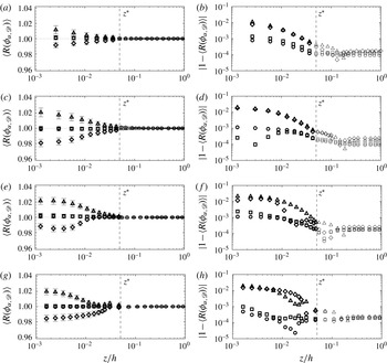
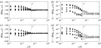
In practice, the renormalization functions, $R({\it\phi}_{{\it\alpha},\mathscr{D}})$ , remain fairly close to unity throughout $0.0\leqslant z/{\it\delta}\leqslant 1$ , and confined to $1\pm 0.001$ for $0.05\leqslant z/{\it\delta}<1$ (see §§ 4.6 and 5.3). With a choice of $z^{\ast }/{\it\delta}=0.05$ and these values of $R({\it\phi}_{{\it\alpha},\mathscr{D}})$ , no significant jump discontinuity occurs at $z=z^{\ast }$ when the solution in each domain is switched from its original velocity field, $\overline{u}_{{\it\alpha},\mathscr{D}}(\boldsymbol{x},t)$ , to the renormalized velocity field, $\overline{u}_{{\it\alpha},\mathscr{D}}^{R}(\boldsymbol{x},t)$ . One could also introduce a blending zone, in which the renormalized and original velocity fields in each domain are gradually blended together. However, we found no particular advantage to introducing such a blending zone, and adopted the simpler approach of switching between the renormalized and original velocity fields at  $z^{\ast }$ .

After application of the renormalization procedure (2.2)–(2.4), the velocity fields, $\overline{u}_{{\it\alpha},\mathscr{D}}^{R}(\boldsymbol{x},t)$ , are no longer divergence free. However, one should note that $\overline{u}_{{\it\alpha},\mathscr{D}}^{R}(\boldsymbol{x},t)$ represent only intermediate velocity fields in between time steps. By the end of each time step, the velocity field in each domain is once again projected onto the divergence-free space as part of the solution for that time step. These divergence-free velocity fields no longer have identical turbulence statistics in the two domains, with the difference between the two sets of statistics being equal to the values of $R({\it\phi}_{{\it\alpha},\mathscr{D}})$ which need to be applied at the next time step. All the mean velocities and LES turbulence intensities reported in the present study were obtained from the divergence-free velocity fields at the conclusion of each time step in the full domain.

3.1 Numerical methods

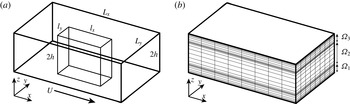
The LES equations (2.1) were solved in the full domain and the minimal flow unit using a patching collocation spectral domain-decomposition method, employing Fourier series in the streamwise ( $x$ ) and spanwise ( $y$ ) directions, and mapped Chebyshev polynomials in the wall-normal ( $z$ ) direction (Orszag Reference Orszag1980; Canuto et al. Reference Canuto, Hussaini, Quarteroni and Zang1988). A schematic of the channel and the coordinate system is shown in figure 1(a). Note that no specific positioning of the minimal flow unit relative to the full domain is required in the nested-LES approach, as the two domains are coupled only through their single-time-averaged turbulence statistics. The computational box spans the full height of the channel, from one wall to the other, in both the full domain and the minimal flow unit, and is partitioned into three non-overlapping sub-domains ${\it\Omega}_{s}$ ( $s=1,2,3$ ) in the wall-normal direction, as shown in figure 1(b). This partitioning allows the grid-point distribution in each zone to be customized to minimize the required number of grid points in the wall-normal direction. 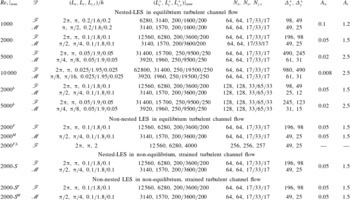The same internal interface locations and wall-normal distribution of grid points were employed in the full domain and the minimal flow unit at each Reynolds number, with the internal interface locations between the ${\it\Omega}_{2}/{\it\Omega}_{1}$ or ${\it\Omega}_{2}/{\it\Omega}_{3}$ sub-domains placed at $z^{+}\approx 200{-}250$ at all Reynolds numbers, as shown in table 1, where the $+$ superscript denotes normalization using inner variables. The continuity of the velocity field, $\overline{u}_{i}$ , and its normal derivative, $\partial \overline{u}_{i}/\partial z$ , were enforced at the internal interfaces between these sub-domains, resulting in solutions which are $C^{1}$ continuous (Canuto et al. Reference Canuto, Hussaini, Quarteroni and Zang1988).

Figure 1.

(a) The computational domains and coordinate system employed in nested-LES of equilibrium and non-equilibrium turbulent channel flows: ——, full domain; ——, minimal flow unit; (b) the patching collocation sub-domains and wall-normal grid distribution employed in both the full domain and minimal flow unit of nested-LES.

Table 1.

Computational domain sizes, grid resolutions, grid spacings and mapping parameters employed in nested-LES and non-nested LES of equilibrium and non-equilibrium turbulent channel flow in the present study.

Algebraic mappings (Kosloff & Talezer Reference Kosloff and Talezer1993) were used to project the ${\it\xi}_{s}\in [-1,1]$ domain of Chebyshev polynomials to the physical domain in the wall-normal direction, in order to maintain the desired distribution of grid points in each sub-domain. The specific algebraic mappings employed in the present study are given by

(3.1) $$\begin{eqnarray}\displaystyle \frac{z}{h} & = & \displaystyle \left(\frac{L_{z,s}}{h}-1\right)-\frac{A_{w}(1-{\it\xi}_{s})}{1+2A_{w}h/L_{z,s}+{\it\xi}_{s}}\qquad \text{for}~s=1,\end{eqnarray}$$

(3.2) $$\begin{eqnarray}\displaystyle \frac{z}{h} & = & \displaystyle \frac{A_{c}{\it\xi}_{s}}{(1+(2A_{c}h/L_{z,s})^{2}-{\it\xi}_{s}^{2})^{1/2}}\qquad \quad \!\,\qquad \text{for}~s=2,\end{eqnarray}$$

(3.3) $$\begin{eqnarray}\displaystyle \frac{z}{h} & = & \displaystyle -\left(\frac{L_{z,s}}{h}-1\right)+\frac{A_{w}(1-{\it\xi}_{s})}{1+2A_{w}h/L_{z,s}+{\it\xi}_{s}}\quad \text{for}~s=3,\end{eqnarray}$$

where $h$ denotes the channel half-height, $L_{z,s}$ denotes the wall-normal height of sub-domain ${\it\Omega}_{s}$ and $A_{w}$ and $A_{c}$ are appropriate scale factors. The specific values of $L_{z,s}$ , $A_{w}$ , and $A_{c}$ for each case are summarized in table 1.

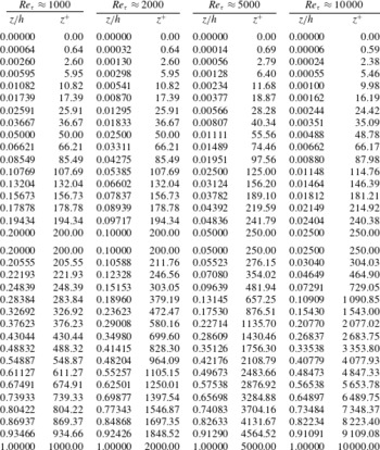
Using the mappings (3.1)–(3.3), nearly the same distribution of grid points in inner scaling ( $+$  units) was maintained in the ${\it\Omega}_{1}$ and ${\it\Omega}_{3}$ sub-domains, with a fixed number of grid points, at all Reynolds numbers, as shown in table 2. Maintaining such a distribution of grid points in the ${\it\Omega}_{1}$ and ${\it\Omega}_{3}$ sub-domains was found to be critical for accurate prediction of the friction coefficient at all Reynolds numbers. Similarly, in the wake region, $z/h>0.3$ , the mappings result in a nearly uniform distribution of grid points in outer ( $z/h$ ) scaling at all Reynolds numbers, as shown in table 2. This makes the required number of grid points in the wake region also independent of Reynolds number for a full domain of a fixed size in outer scaling. In the logarithmic region ( $z^{+}>3Re_{{\it\tau}}^{1/2}$ and $z/h<0.3$ ) (Marusic et al. Reference Marusic, Monty, Hultmark and Smits2013; Meneveau & Marusic Reference Meneveau and Marusic2013), where the size of the eddies grows in proportion to the distance from the wall, the required number of grid points has a weak dependence on $Re_{{\it\tau}}$ , and grows as $\log (Re_{{\it\tau}})$ , as shown in § 6. Because of the weak, logarithmic, nature of this dependence on $Re_{{\it\tau}}$ , computations can be performed with a fixed number of grid points in the wall-normal direction over nearly a decade of $Re_{{\it\tau}}$ values in this region as well, which is the approach adopted in the present study. With such a distribution of grid points, the near-wall region is well resolved in both the minimal flow unit and the full domain, and both domains can be solved subject to the no-slip boundary conditions at the walls, without the need for any wall models.

Table 2.

Wall-normal grid distribution employed in nested-LES and non-nested LES of equilibrium and non-equilibrium turbulent channel flow at $Re_{{\it\tau}}\approx 1000$ , 2000, 5000 and 10 000 at ‘standard’ resolution.

The LES governing equations were integrated in time using a second-order fractional-step method, with explicit treatment of the nonlinear terms using an Adams–Bashforth scheme, and semi-implicit treatment of the pressure–viscous terms using a Crank–Nicolson scheme (Yakhot et al. Reference Yakhot, Orszag, Yakhot and Israeli1989). All the simulations were de-aliased using the so-called $2/3$ rule (Canuto et al. Reference Canuto, Hussaini, Quarteroni and Zang1988), and were initialized from an LES database of a fully developed turbulent channel flow at $Re_{{\it\tau}}\approx 570$ . A constant flow rate (per unit width) was maintained in both the full domain and minimal flow unit throughout the course of all simulations.

3.2 Simulation parameters

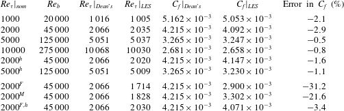
The simulations of equilibrium turbulent channel flow were performed at bulk Reynolds numbers, $Re_{b}\equiv U_{b}h/{\it\nu}$ , of 20 000, 45 000, 125 000 and 275 000, corresponding to friction Reynolds numbers, $Re_{{\it\tau}}\equiv u_{{\it\tau}}h/{\it\nu}$ , of 1016, 2066, 5051 and 10 068, respectively, based on the $u_{{\it\tau}}$ from Dean’s correlation (Dean Reference Dean1978). Throughout this study, these cases will be referred to as ‘nominal’ $Re_{{\it\tau}}\approx 1000$ , 2000, 5000 and 10 000, respectively, as shown in table 1.

Figure 2.

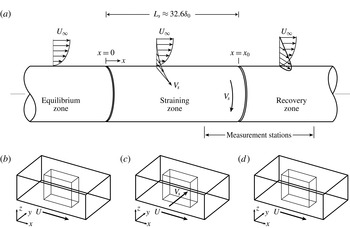
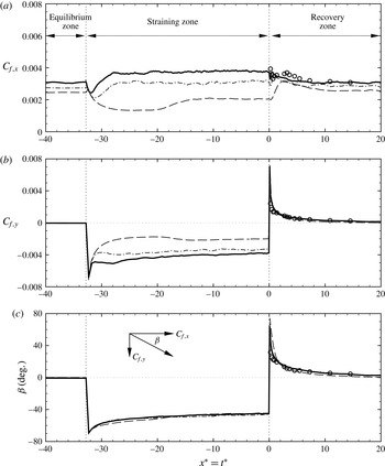
(a) Schematic of the experimental set-up of shear driven, three-dimensional turbulent boundary layer by Driver & Hebbar (Reference Driver and Hebbar1991); (b–d) schematic of the channel flows used in nested-LES of non-equilibrium, strained channel flow in each of the equilibrium, straining and recovery zones in the present study.

The simulations of non-equilibrium, strained turbulent channel flow were designed to emulate the experimental conditions of Driver & Hebbar (Reference Driver and Hebbar1991), in which an initially two-dimensional turbulent boundary layer (TBL) at $Re_{{\it\theta}}\approx 6900$ ( $Re_{{\it\tau}}\approx 2000$ ) was driven to three-dimensionality by impulsive transverse motion of the wall at speed $V_{s}=U_{\infty }$ over a length $L_{s}\approx 32.6{\it\delta}_{0}$ , followed by cessation of the transverse motion of the wall, and recovery to initial two-dimensional state, as shown in figure 2(a). Here, $U_{\infty }$ denotes the free-stream velocity in the original TBL, ${\it\delta}_{0}$ denotes the boundary layer thickness at the end of the shearing zone and $L_{s}$ denotes the length of the shearing zone. In the large-eddy simulations, a fully developed, equilibrium turbulent channel flow at $Re_{{\it\tau}}\approx 2000$ is subjected to impulsive transverse motion of one of the walls at speed $V_{s}=U_{c}$ for a time period $T_{s}$ , followed by cessation of the transverse motion of the wall, and recovery to equilibrium turbulent channel flow, where $U_{c}$ denotes the mean centreline velocity in the initial equilibrium turbulent channel. The correspondence between ‘time’ in the simulations and ‘position’ in the experiments was computed based on Taylor’s hypothesis,

(3.4) $$\begin{eqnarray}\frac{tU_{c}}{h}=\frac{x}{{\it\delta}(x)},\end{eqnarray}$$

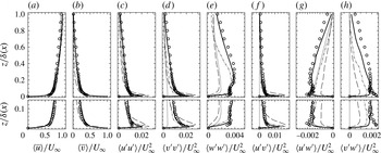
where $t$ is the time from the start of the transverse motion of the lower wall in the simulations, $x$ denotes the streamwise distance from the leading edge of the moving wall section in the experiments (see figure 2 a) and ${\it\delta}(x)$ is the local boundary thickness in the experiments. The evolution of turbulence statistics from equilibrium channel flow to strained, non-equilibrium flow, and recovery back to equilibrium turbulent channel flow was tracked in LES and compared to experimental measurements (Driver & Hebbar Reference Driver and Hebbar1991). In comparing the turbulence statistics from TBL experiments to LES predictions in turbulent channel flow, the normalized wall-normal location, $z/{\it\delta}(x)$ , mean velocities, $\langle \overline{u}_{i}\rangle /U_{\infty }$ and turbulent stresses, $\langle u_{i}^{\prime }u_{j}^{\prime }\rangle /U_{\infty }^{2}$ , from the TBL were equated with $z/h$ , $\langle \overline{u}_{i}\rangle /U_{c}$ , and $\langle u_{i}^{\prime }u_{j}^{\prime }\rangle /U_{c}^{2}$ in channel flow, respectively.

All the simulations of equilibrium and non-equilibrium channel flow were performed in full domains of size $L_{x}\times L_{y}\times L_{z}=2{\rm\pi}h\times {\rm\pi}h\times 2h$ , and minimal flow units of size $l_{x}^{+}\approx 3200{-}3900$ , $l_{y}^{+}\approx 1600{-}1950$ , and $l_{z}=2h$ , in the streamwise, spanwise and wall-normal directions, respectively, as shown in table 1. The size of the minimal flow unit in the homogeneous flow directions was chosen to accommodate ${\sim}3{-}4$ near-wall structures in the streamwise, and ${\sim}15{-}20$ near-wall structures in the spanwise directions, to provide a reasonably adequate ensemble for the single-time averages employed in the decomposition and renormalization procedures of (2.2)–(2.4). Grid resolutions of $64\times 64\times 17/33/17$ were employed in both the full domain and the minimal flow unit as the standard resolution in all the simulations, independent of the Reynolds number. With these domains sizes and grid resolutions, grid spacings of ${\it\Delta}_{x}^{+}\approx 50{-}60$ in the streamwise and ${\it\Delta}_{y}^{+}\approx 25{-}30$ in the spanwise direction are maintained in the minimal flow unit at all Reynolds numbers, while in the full domain, grid spacings of ${\it\Delta}_{x}/h=2{\rm\pi}/64\approx 0.1$ in the streamwise and ${\it\Delta}_{y}/h={\rm\pi}/64\approx 0.05$ in the spanwise direction are maintained at all Reynolds numbers. In the wall-normal direction, the same grid distribution is used in the full domain and minimal flow unit at each Reynolds number. The specific grid distributions employed at each Reynolds number are shown in table 2. With the aid of the patching collocation method and the mappings discussed in § 3.1, a nearly fixed distribution of grid points in inner scaling ( $+$  units) is maintained in the near-wall region ( $0\leqslant z^{+}\leqslant 200{-}250$ ) at all Reynolds numbers to resolve the near-wall region down to the viscous sublayer and the wall, as shown in table 2. In the wake region, $z/h>0.3$ , the patching collocation method and the mappings discussed in § 3.1 result in nearly uniform grid spacings of ${\it\Delta}_{z}/h\approx 0.05{-}0.1$ at all Reynolds numbers, while in the logarithmic region, between $z^{+}\geqslant 3Re_{{\it\tau}}^{1/2}$ and $z/h\leqslant 0.3$ , the grid size almost linearly increases from its value in the near-wall sub-domain to its values in the wake region.

In addition to these ‘standard resolution’ cases, nested-LES of equilibrium turbulent channel flow at $Re_{{\it\tau}}\approx 2000$ and 5000 were performed with double the resolution in each direction, to verify the grid independence of the results. These cases, which were performed with grid resolutions of $128\times 128\times 33/65/33$ , are denoted by cases $2000^{h}$ and $5000^{h}$ in table 1.

Furthermore, to assess the effectiveness of the nested-LES approach, a set of non-nested large-eddy simulations were performed in equilibrium and non-equilibrium turbulent channel flows at $Re_{{\it\tau}}\approx 2000$ in domains of the same size as the full domain and minimal flow unit of the nested-LES, with the same grid resolutions as those employed in nested-LES. These cases are denoted by $2000^{F}$ , $2000^{M}$ , 2000- $S^{F}$ , 2000- $S^{M}$ in table 1, representing non-nested equilibrium channel flow in the full domain, non-nested equilibrium channel flow in the minimal flow unit, non-nested sheared channel flow in the full domain and non-nested sheared channel flow in the minimal flow unit, respectively.

The turbulence statistics reported in equilibrium turbulent channel flow were obtained by ensemble averaging the flow quantities in space, over the homogeneous flow directions, and in time, over approximately ten eddy turnover times, $h/u_{{\it\tau}}$ . The turbulence statistics reported in the non-equilibrium, strained turbulent channel flow were obtained by ensemble averaging the flow quantities in space, over the homogeneous flow directions and over ten independent realizations of the strained turbulent channel flow, each initialized from a different nested-LES realization of a fully developed, equilibrium turbulent channel flow at $Re_{{\it\tau}}\approx 2000$ .

3.3 SGS model and reconstruction of RANS turbulence statistics

The conventional approach to modelling the term $\overline{u_{i}u_{j}}$ in (2.1) is to represent it as $\overline{u_{i}u_{j}}=\overline{u}_{i}\overline{u}_{j}+{\it\tau}_{ij}$ , and model the subgrid-scale stress tensor, ${\it\tau}_{ij}\equiv \overline{u_{i}u_{j}}-\overline{u}_{i}\overline{u}_{j}$ (Sagaut & Meneveau Reference Sagaut and Meneveau2006). This choice, however, is not unique, and some investigators have favoured representing $\overline{u_{i}u_{j}}$ as $\overline{u_{i}u_{j}}=\overline{\overline{u}_{i}\overline{u}_{j}}+\overline{A}_{ij}$ and modelling $\overline{A}_{ij}$ (Winckelmans, Jeanmart & Carati Reference Winckelmans, Jeanmart and Carati2002) or even modelling $\overline{u_{i}u_{j}}$ directly (Haliloglu & Akhavan Reference Haliloglu, Akhavan, Geurts, Metais and Freidrich2004). The implementation of the nested-LES approach is independent of all such modelling issues. Nested-LES can be applied with any formulation of $\overline{u_{i}u_{j}}$ , and any SGS model of choice.

In this study, the conventional definition of SGS stress, along with the dynamic Smagorinsky model (DSM) of Germano et al. (Reference Germano, Piomelli, Moin and Cabot1991) and Lilly (Reference Lilly1992) with sharp, spectral, cutoff filters has been used, because of its known performance characteristics and simplicity. Following the original formulation of Germano et al. (Reference Germano, Piomelli, Moin and Cabot1991) and Lilly (Reference Lilly1992), the implicit spectral cutoff LES filters were placed at the de-aliased grid filter location. Test filtering was applied only in the streamwise and spanwise directions, and the test filters were placed at half the implicit LES filter locations.

In LES, only the filtered velocity, $\overline{u}_{i}$ , is computed. Consequently, the turbulent stresses, $\langle \overline{u}_{i}^{\prime }\overline{u}_{j}^{\prime }\rangle$ , computed in LES, are not the true RANS stresses, $\langle u_{i}^{\prime }u_{j}^{\prime }\rangle$ . Here, $\overline{u}_{i}^{\prime }=\overline{u}_{i}-\langle \overline{u}_{i}\rangle$ denotes the fluctuating velocity field in LES, $u_{i}^{\prime }=u_{i}-\langle u_{i}\rangle$ denotes the RANS fluctuating velocity field, $\overline{u}_{i}$ is the velocity field resolved in LES, $u_{i}$ is the full velocity field and $\langle ~\rangle$ denotes an ensemble average in the spatially homogeneous flow directions and in time. To allow meaningful comparisons between the LES results and the RANS turbulence statistics reported in DNS or experiments, the RANS turbulent stresses were recovered from the turbulent stresses computed in LES using the formulation (Voelkl, Pullin & Chan Reference Voelkl, Pullin and Chan2000; Winckelmans et al. Reference Winckelmans, Jeanmart and Carati2002),

(3.5) $$\begin{eqnarray}\langle u_{i}^{\prime }u_{j}^{\prime }\rangle \simeq \langle \overline{u}_{i}^{\prime }\overline{u}_{j}^{\prime }\rangle +\langle {\it\tau}_{ij}^{\ast }\rangle +{\textstyle \frac{2}{3}}{\it\delta}_{ij}K_{sgs},\end{eqnarray}$$

where ${\it\tau}_{ij}^{\ast }={\it\tau}_{ij}-{\it\delta}_{ij}{\it\tau}_{kk}/3$ denotes the deviatoric part of the SGS stress tensor, and $K_{sgs}\equiv \langle {\it\tau}_{kk}\rangle /2$ is the SGS kinetic energy.

Application of (3.5) requires knowledge of $K_{sgs}$ . In LES of incompressible flow, ${\it\tau}_{kk}$ can be lumped together with the pressure term and solved for implicitly during the course of the simulation. Consequently, most existing SGS models, such as DSM, model only the deviatoric part of the SGS stress tensor and provide no information on ${\it\tau}_{kk}$ . With such models, the SGS kinetic energy is not directly available from LES, and needs to be recovered at a post-processing stage. In this study, the SGS kinetic energy was recovered from the continuation of the one-dimensional (1-D) energy spectra obtained in LES at each wall-normal location, using an analytical formulation of the 1-D energy spectra in wall flows (Tang & Akhavan Reference Tang, Akhavan and Eckhardt2009; Tang Reference Tang2015) derived based on Pao’s formulation of the three-dimensional (3-D) spectrum for isotropic turbulence (Pao Reference Pao1965). These analytical 1-D spectra were used to ‘continue’ the 1-D energy spectra from LES down to the Kolmogorov scale. The SGS kinetic energy was then recovered by integrating the areas under these ‘continued’ spectra. A similar approach for recovery of the SGS kinetic energy has previously been employed in homogeneous, isotropic turbulence based on analytical or empirical formulations of the 3-D spectra in isotropic turbulence (Knaepen, Debliquy & Carati Reference Knaepen, Debliquy and Carati2002; Meyers & Baelmans Reference Meyers and Baelmans2004). All the SGS kinetic energies used for the reconstruction of the RANS turbulent intensities, and the Reynolds shear stresses reported in the present study, were obtained from the spectra and velocity fields in the full domain for $z>z^{\ast }$ , and from the spectra and velocity fields in the minimal flow unit for $z\leqslant z^{\ast }$ , to take advantage of the additional resolution available in the minimal flow unit for $z\leqslant z^{\ast }$ .

4.1 Mean statistics

Table 3 shows the skin friction coefficients, $C_{f}\equiv \langle 2{\it\tau}_{w}\rangle /{\it\rho}U_{b}^{2}$ , predicted by nested-LES in equilibrium turbulent channel flow, at standard and high resolutions, compared to Dean’s correlation (Dean Reference Dean1978). The predicted skin friction coefficients were within $-2.1\,\%$ , $-2.9\,\%$ , $-0.5\,\%$ and $-0.8\,\%$ of values from Dean’s correlation at $Re_{{\it\tau}}\approx 1000$ , 2000, 5000 and 10 000, respectively, with standard resolution, and within $-2\,\%$ of the values from Dean’s correlation in the high-resolution simulations of $2000^{h}$ and $5000^{h}$ .

Table 3.

The skin friction coefficient, $C_{f}$ , predicted in nested-LES and non-nested LES of equilibrium turbulent channel flow compared to Dean’s correlation (Dean Reference Dean1978).

The profiles of the mean velocity, turbulence intensities and Reynolds shear stresses predicted by nested-LES in these flows are shown in figure 3. The mean velocity profiles predicted at $Re_{{\it\tau}}\approx 1000$ , 2000 and 5000 show good agreement with available DNS data at $Re_{{\it\tau}}\approx 950$ (del Alamo et al. Reference del Alamo, Jimenez, Zandonade and Moser2004), $Re_{{\it\tau}}\approx 2000$ (Hoyas & Jimenez Reference Hoyas and Jimenez2006), $Re_{{\it\tau}}\approx 5200$ (Lee & Moser Reference Lee and Moser2015) and experimental data at $Re_{{\it\tau}}\approx 4800$ (Comte-Bellot Reference Comte-Bellot1963), respectively. At $Re_{{\it\tau}}\approx 10\,000$ , no DNS data is currently available. Consequently, the nested-LES results were assessed based on a combination of DNS data at $Re_{{\it\tau}}\approx 5200$ (Lee & Moser Reference Lee and Moser2015) and experimental data at $Re_{{\it\tau}}\approx 8600$ (Comte-Bellot Reference Comte-Bellot1963). The original experimental data at $Re_{{\it\tau}}\approx 8600$ published by Comte-Bellot (Reference Comte-Bellot1963) displays a mean velocity profile which is shifted relative to the universal law of the wall. In the present study, this experimental data is displayed after adjusting the value of the wall friction velocity, $u_{{\it\tau}}$ , in the experiments to bring the experimental data into agreement with the universal law of the wall. All the experimental data of Comte-Bellot (Reference Comte-Bellot1963) at $Re_{{\it\tau}}\approx 8600$ shown in the present study have been normalized using this adjusted  $u_{{\it\tau}}$ .

Figure 3.

Profiles of the mean velocity, turbulence intensities and Reynolds shear stress predicted by nested-LES in equilibrium turbulent channel flow at (a–c)  $Re_{{\it\tau}}\approx 1000$ , (d–f)  $Re_{{\it\tau}}\approx 2000$ , (g–i)  $Re_{{\it\tau}}\approx 5000$ , (j–l)  $Re_{{\it\tau}}\approx 10\,000$ , compared to DNS and experimental data. ——, nested-LES performed at standard resolution;  

(orange), nested-LES cases of $2000^{h}$ and $5000^{h}$ , performed at high resolution; thick lines, mean velocity, RANS turbulence intensities, $\langle u_{{\it\alpha}}^{\prime }u_{{\it\alpha}}^{\prime }\rangle ^{1/2}$ , and Reynolds shear stress, $\langle u^{\prime }w^{\prime }\rangle$ , reconstructed from nested-LES results using (3.5); thin lines, turbulence intensities, $\langle \overline{u}_{{\it\alpha}}^{\prime }\overline{u}_{{\it\alpha}}^{\prime }\rangle ^{1/2}$ , and Reynolds shear stress, $\langle \overline{u}^{\prime }\overline{w}^{\prime }\rangle$ , predicted by nested-LES without reconstruction; ▫, DNS at $Re_{{\it\tau}}\approx 950$ (del Alamo et al. Reference del Alamo, Jimenez, Zandonade and Moser2004); ○, DNS at $Re_{{\it\tau}}\approx 2000$ (Hoyas & Jimenez Reference Hoyas and Jimenez2006); ♢, DNS at $Re_{{\it\tau}}\approx 5200$ (Lee & Moser Reference Lee and Moser2015); ▵, experiments at $Re_{{\it\tau}}\approx 4800$ (Comte-Bellot Reference Comte-Bellot1963); ▿, experiments at $Re_{{\it\tau}}\approx 8600$ (Comte-Bellot Reference Comte-Bellot1963);  ${-}\,\cdot \cdot \,\,{-}$ , LES at $Re_{{\it\tau}}\approx 4000$ (Kravchenko, Moin & Moser Reference Kravchenko, Moin and Moser1996);  $\cdots \cdots$ , the asymptotes $\langle \overline{u}\rangle ^{+}=z^{+}$ , and $\langle \overline{u}\rangle ^{+}=2.5\ln (z^{+})+5$ .

The mean velocity profiles predicted by nested-LES exhibit the correct behaviour throughout the cross-section of the channel at all Reynolds numbers, including the correct slope in the logarithmic layer, and agreement with DNS and experimental data in the wake region. Furthermore, no change in slope or other anomalies are observed in the mean velocity profiles at $z=z^{\ast }$ . The high-resolution cases of $2000^{h}$ and $5000^{h}$ predict mean velocity profiles which are virtually indistinguishable from those obtained at standard resolution, consistent with the close agreement between the $C_{f}$ values of the standard- and high-resolution cases.

Good agreement is also observed in figure 3 between the turbulence intensities and Reynolds shear stresses predicted by nested-LES and available DNS and experimental data. To allow direct comparison of the nested-LES predictions with available DNS and experimental data, the true RANS turbulence intensities, $\langle u_{{\it\alpha}}^{\prime }u_{{\it\alpha}}^{\prime }\rangle ^{1/2}$ , were reconstructed from the LES results using (3.5) and shown in figure 3. For reference, the LES turbulence intensities, $\langle \overline{u}_{{\it\alpha}}^{\prime }\overline{u}_{{\it\alpha}}^{\prime }\rangle ^{1/2}$ , without reconstruction are also shown. Unlike most existing wall modelling approaches, which only provide the turbulence statistics in the outer layer, the nested-LES approach can provide accurate predictions of the turbulent statistics in both the inner and outer layers. Both the locations and magnitudes of the near-wall peaks of the turbulence intensities are accurately predicted at all Reynolds numbers, with the magnitude of the near-wall peak of the streamwise turbulence intensity showing a gradual increase with increasing Reynolds number, consistent with recent observations in experiments (Marusic et al. Reference Marusic, Mckeon, Monkewitz, Nagib, Smits and Sreenivasan2010b ) and DNS (Hoyas & Jimenez Reference Hoyas and Jimenez2006; Schlatter et al. Reference Schlatter, Li, Brethouwer, Johansson and Henningson2010). The overprediction of the near-wall peak of the streamwise turbulence intensity by 3–7 % at standard resolution, and by less than 1 % at high resolution, and underprediction of the streamwise turbulence intensities in the logarithmic layer by up to 10–15 % at both resolutions, observed in figure 3 compared to DNS, are both features of DSM which have also been observed in a number of prior studies. An example of such studies, performed with DSM using well-resolved conventional LES at $Re_{{\it\tau}}\approx 4000$ (Kravchenko et al. Reference Kravchenko, Moin and Moser1996; Cabot & Moin Reference Cabot and Moin1999), is also shown in figure 3(g–i). Similar differences of up to 5 %, 10 % and 5 % at standard resolution, and up to 3 %, 6 % and 2 % at high resolution, are also observed in figure 3 in the prediction of the spanwise and wall-normal turbulent intensities and the Reynolds shear stress, respectively, compared to DNS.

The high-resolution cases of $2000^{h}$ and $5000^{h}$ predict reconstructed RANS turbulence intensities and a Reynolds shear stress within 5 % of the results from the standard resolution for $z^{+}\leqslant 200$ , and within 2 % of the results from the standard resolution in the rest of the channel, indicating the invariance of the results to the resolution of the grid.

Recovery of the SGS stresses leads to differences of up to 5 %, 12 % and 16 %, at standard resolution, and up to 3 %, 8 % and 12 % at high resolution, between the RANS and LES turbulence intensities in the streamwise, spanwise and wall-normal directions, respectively.

4.2 Energy spectra

Figure 4 shows the 1-D energy spectra of the components of the fluctuating velocity predicted by nested-LES in turbulent channel flow at $1000\leqslant Re_{{\it\tau}}\leqslant 10\,000$ in the outer layer ( $z/h\approx 0.5$ ) and near-wall region ( $z^{+}\approx 20$ ), compared to DNS data of Hoyas & Jimenez (Reference Hoyas and Jimenez2006) at $Re_{{\it\tau}}\approx 2000$ . The nested-LES spectra are normalized using the kinematic viscosity, ${\it\nu}$ , and plane-averaged rates of TKE dissipation, defined as $\langle {\it\epsilon}\rangle \equiv \langle 2{\it\nu}\overline{s}_{ij}^{\prime }\overline{s}_{ij}^{\prime }+\overline{s}_{ij}^{\prime }{\it\tau}_{ij}\rangle$ , where $\overline{s}_{ij}^{\prime }=(\partial \overline{u}_{i}^{\prime }/\partial x_{j}+\partial \overline{u}_{j}^{\prime }/\partial x_{i})/2$ is the resolved fluctuating strain rate tensor, ${\it\tau}_{ij}$ is the modelled SGS stress tensor and $\langle ~\rangle$ denotes ensemble averaging in space, over the homogeneous flow directions, and in time.

Figure 4.

One-dimensional energy spectra of the streamwise, spanwise, and wall-normal velocity fluctuations, predicted by nested-LES in equilibrium turbulent channel flow at $1000\leqslant Re_{{\it\tau}}\leqslant 10\,000$ in (a–f) outer region ( $z/h\approx 0.5$ ), (g–l) near-wall region ( $z^{+}\approx 20$ ): (a–c,g–i), energy spectra in the streamwise direction; (d–f,j–l), energy spectra in the spanwise direction.  

,  $Re_{{\it\tau}}\approx 1000$ ;  

,  $Re_{{\it\tau}}\approx 2000$ ;  

,  $Re_{{\it\tau}}\approx 5000$ ; ——, $Re_{{\it\tau}}\approx 10\,000$ ;  

 (orange),  $Re_{{\it\tau}}\approx 2000^{h}$ high resolution;  

 (orange), $Re_{{\it\tau}}\approx 5000^{h}$ high resolution; thick lines, spectra in the full domain of nested-LES; thin lines, spectra in the minimal flow unit of nested-LES; ○, DNS at $Re_{{\it\tau}}\approx 2000$ (Hoyas & Jimenez Reference Hoyas and Jimenez2006).

In the outer layer ( $z/h\approx 0.5$ ), the full-domain spectra span the range of scales from the largest eddies in the computational domain down to inertial-range eddies, while the minimal-flow-unit spectra span the range of scales from inertial-range eddies down to dissipation-range eddies. The full-domain spectra display a region conforming to ${\sim}k^{-5/3}$ asymptote in the inertial range, and a Reynolds number dependent peel-off from the $k^{-5/3}$ asymptote in the energy-containing scales, as anticipated. The largest scales of the minimal flow unit, which fall in the inertial range, also have a ${\sim}k^{-5/3}$ asymptote, but are shifted relative to the inertial range of the full domain because these scales need to absorb the energy in the energy-containing scales of the full domain which are absent in the minimal flow unit. At the small scales, the minimal-flow-unit spectra display a drop-off in the dissipation range which is sharper than that in DNS due to the presence of SGS dissipation in nested-LES. With decreasing Reynolds number or increasing resolution, as in high resolution cases of $2000^{h}$ and $5000^{h}$ , the dissipation-range spectra begin to approach those in DNS. In the energy-containing and inertial-range scales, the predicted spectra for cases 5000 and $5000^{h}$ show good agreement with each other, while those for cases 2000 and $2000^{h}$ show good agreement with each other and with DNS data (Hoyas & Jimenez Reference Hoyas and Jimenez2006).

In the near-wall region ( $z^{+}\approx 20$ ), the spectra in the minimal flow unit at different Reynolds numbers and different resolutions all collapse and agree with DNS, reflecting the presence of sufficient resolution in the minimal flow unit of nested-LES in the near-wall region. The full-domain spectra in the near-wall region capture the large-scale features observed in the DNS spectra, and show an upshift of the spectra in the largest scales with increasing Reynolds number.

4.3 High-order moments

Recent experiments in high Reynolds number turbulent boundary layers and pipe flows (Hultmark et al. Reference Hultmark, Vallikivi, Bailey and Smits2013; Marusic et al. Reference Marusic, Monty, Hultmark and Smits2013; Meneveau & Marusic Reference Meneveau and Marusic2013) have confirmed that the variance of the streamwise velocity fluctuations exhibits logarithmic behaviour within an inertial sublayer, consistent with, and supportive of, earlier predictions by models based on the ‘attached-eddy’ hypothesis (Townsend Reference Townsend1976; Perry, Henbest & Chong Reference Perry, Henbest and Chong1986). It has further been shown (Meneveau & Marusic Reference Meneveau and Marusic2013) that this logarithmic behaviour can be generalized to all even-order moments of the streamwise velocity fluctuations as,

(4.1) $$\begin{eqnarray}\langle (u^{\prime +})^{2p}\rangle ^{1/p}=-A_{p}\ln (z/{\it\delta})+B_{p}=-A_{p}\ln (z^{+})+D_{p}(Re_{{\it\tau}}),\end{eqnarray}$$

where the coefficients $A_{p}$ are the generalized ‘Townsend–Perry’ constants for moments of order $2p$ , and appear quite insensitive to the Reynolds number, while $B_{p}$ and $D_{p}$ are non-universal constants.

It has been suggested that the ability of LES to reproduce this logarithmic behaviour in the higher-order moments of the streamwise velocity fluctuations, with generalized ‘Townsend–Perry’ constants, $A_{p}$ , in agreement with experiments, should be used as an additional criterion for evaluation of the capability of LES to capture the fundamental scaling laws and inherent nonlinear dynamics of turbulence (Stevens, Wilczek & Meneveau Reference Stevens, Wilczek and Meneveau2014). Furthermore, it has been reported that for wall-modelled conventional LES to faithfully reproduce these generalized ‘Townsend–Perry’ constants, a fine resolution is required in the simulations (Stevens et al. Reference Stevens, Wilczek and Meneveau2014).

In this section, we explore the ability of the nested-LES approach to predict this logarithmic behaviour in the even-order moments of the streamwise velocity fluctuations. Figure 5(a,b) show the second ( $2p=2$ ) and sixth ( $2p=6$ ) order moments of the streamwise velocity fluctuations, $\langle (u^{\prime +})^{2p}\rangle ^{1/p}$ , predicted by nested-LES at $1000\leqslant Re_{{\it\tau}}\leqslant 10\,000$ , respectively, while figure 5(c) shows the even-order moments for $2\leqslant 2p\leqslant 12$ at $Re_{{\it\tau}}=10\,000$ . A logarithmic behaviour can be observed in all the even-order moments displayed in figure 5(a–c) over the range $z^{+}>3Re^{1/2}$ and $z/h<0.30$ , for which the logarithmic behaviour has been observed in experiments (Marusic et al. Reference Marusic, Monty, Hultmark and Smits2013; Meneveau & Marusic Reference Meneveau and Marusic2013). The data shown in figure 5(c) indicates that the logarithmic behaviour may extend beyond $z/h\sim 0.3$ with increasing order of the moments. Nevertheless, the coefficients $A_{p}$ and $D_{p}$ in (4.1) were obtained by a least squares fit to the moments between $z^{+}>3Re^{1/2}$ and $z/h<0.30$ .

Figure 5.

Moments of order (a) $2p=2$ , (b) $2p=6$ , (c)  $2p=2$ , 4, 6, 8, 10, 12 (raised to the power of $1/p$ ) of the streamwise velocity fluctuations, (d) coefficients, $A_{p}$ , in the logarithmic law for moments, as a function of the moment order, $2p$ , predicted by nested-LES at $1000\leqslant Re_{{\it\tau}}\leqslant 10\,000$ .  

,  $Re_{{\it\tau}}\approx 1000$ ;  

,  $Re_{{\it\tau}}\approx 2000$ ;  

,  $Re_{{\it\tau}}\approx 5000$ ; ——,  $Re_{{\it\tau}}\approx 10\,000$ ;  

 (orange),  $Re_{{\it\tau}}\approx 2000^{h}$ high-resolution;  

 (orange), $Re_{{\it\tau}}\approx 5000^{h}$ high-resolution;  

 (blue), experiments in TBL at $Re_{{\it\tau}}\approx 19030$ (Meneveau & Marusic Reference Meneveau and Marusic2013);  $\cdots \times \cdots$ , Gaussian values for $A_{p}=A_{1}[(2p-1)!!]^{1/p}$ with $A_{1}=1.25$ ; $\cdots \cdots$ , logarithmic fit to the region $3Re_{{\it\tau}}^{1/2}\leqslant z^{+}\leqslant 0.3Re_{{\it\tau}}$ ; the dashed vertical lines in (a–c) denote the bounds of the region $3Re_{{\it\tau}}^{1/2}\leqslant z^{+}\leqslant 0.3Re_{{\it\tau}}$ .

Figure 5(d) shows the values of the coefficients $A_{p}$ , for $2\leqslant 2p\leqslant 12$ , obtained from nested-LES results at $1000\leqslant Re_{{\it\tau}}\leqslant 10\,000$ . For reference, the $A_{p}$ coefficients from experimental measurements in TBL at $Re_{{\it\tau}}\approx 19\,030$ (Meneveau & Marusic Reference Meneveau and Marusic2013) are also shown. The $A_{p}$ coefficients obtained from nested-LES at $Re_{{\it\tau}}\approx 10\,000$ show good agreement with the $A_{p}$ coefficients from TBL experiments at $Re_{{\it\tau}}\approx 19\,030$ , indicating the insensitivity of the $A_{p}$ coefficients to the Reynolds number at high enough Reynolds numbers. At low Reynolds numbers ( $Re_{{\it\tau}}\leqslant 2000$ ), the trends in $A_{p}$ coefficients from nested-LES are similar to those observed at low Reynolds numbers in experiments (Meneveau & Marusic Reference Meneveau and Marusic2013). At all Reynolds numbers, the $A_{p}$ coefficients from both nested-LES and experiments show sub-Gaussian behaviour. The limiting asymptotic behaviour of the $A_{p}$ coefficient at high Reynolds numbers indicates that this sub-Gaussian scaling of the moments does not become more Gaussian with increasing Reynolds number.

Figure 6.

Skewness (a–f), and flatness (g–l) of the streamwise (a,d,g,j), spanwise (b,e,h,k) and wall-normal (c,f,i,l) velocity fluctuations as a function of $z^{+}$ (a–c,g–i), and $z/h$ (d–f,j–l). Line types as in figure 4.

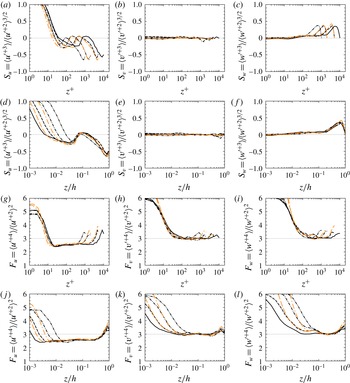
Further evidence of the sub-Gaussian behaviour of the streamwise velocity fluctuations is observed in the plots of skewness and flatness, as shown in figure 6. Both the skewness and flatness of the streamwise velocity fluctuations display sub-Gaussian behaviour in the logarithmic region. A sign change is observed in the skewness of the streamwise velocity fluctuations in the inner layer ( $z/h<0.1$ ). A similar sign change in the sign of $S_{u}$ has been reported experimentally, but only in the buffer layer and of much weaker negative magnitude (Marusic, Mathis & Hutchins Reference Marusic, Mathis and Hutchins2010a ). The profiles of the flatness of the streamwise velocity fluctuations show similar trends to experiments in TBL (Meneveau & Marusic Reference Meneveau and Marusic2013). The spanwise velocity fluctuations display near-Gaussian behaviour throughout the logarithmic layer, with skewness and flatness values near the Gaussian values of 0 and 3, respectively. The wall-normal velocity fluctuations display slightly super-Gaussian behaviour with a slightly positive skewness and flatness values slightly higher than the Gaussian values.

4.4 Two-point statistics

The previous sections have established the ability of nested-LES to faithfully predict the one-point statistics and spectra in turbulent channel flow. In this section, we investigate the ability of nested-LES to predict structural features of the flow. To this end, we examine the two-point correlations obtained from nested-LES in turbulent channel flow.

The two-point correlation coefficient, $C_{{\it\varphi}{\it\varphi}}$ , is defined as

(4.2) $$\begin{eqnarray}C_{{\it\varphi}{\it\varphi}}(\boldsymbol{r},\boldsymbol{r}^{\prime })=\frac{\langle {\it\varphi}(\boldsymbol{r}){\it\varphi}(\boldsymbol{r}^{\prime })\rangle }{{\it\sigma}_{{\it\varphi}}(\boldsymbol{r}){\it\sigma}_{{\it\varphi}}(\boldsymbol{r}^{\prime })},\end{eqnarray}$$

where ${\it\varphi}$ denotes the streamwise, spanwise or wall-normal velocity fluctuations, $\boldsymbol{r}=(x,y,z)$ and $\boldsymbol{r}^{\prime }=(x^{\prime },y^{\prime },z^{\prime })$ are the coordinates of the reference point and the moving point, respectively, $\langle ~\rangle$ denotes ensemble averaging in time and in homogeneous directions, and ${\it\sigma}_{{\it\varphi}}(\boldsymbol{r})$ and ${\it\sigma}_{{\it\varphi}}(\boldsymbol{r}^{\prime })$ are the standard deviations of ${\it\varphi}$ evaluated at $\boldsymbol{r}$ and $\boldsymbol{r}^{\prime }$ , respectively.

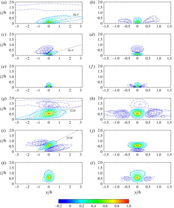
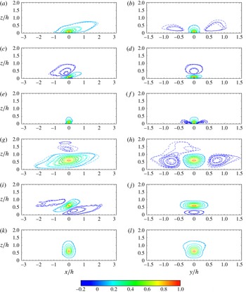
Figure 7 shows the streamwise ( $x$ – $z$ plane) and spanwise ( $y$ – $z$ plane) sections of the contour maps of $C_{uu}$ , $C_{vv}$ , $C_{ww}$ at $z/h=0.1$ and $z/h=0.6$ , based on data from nested-LES at $1000\leqslant Re_{{\it\tau}}\leqslant 10\,000$ . The contour maps of the correlation coefficients at different Reynolds numbers show a reasonable collapse, with the exception of the weakly correlated structures of $C_{uu}$ . This lack of a simple Reynolds number scaling for the $C_{uu}$ structures has been reported in several prior studies (del Alamo et al. Reference del Alamo, Jimenez, Zandonade and Moser2004; Jimenez & Hoyas Reference Jimenez and Hoyas2008; Sillero, Jimenez & Moser Reference Sillero, Jimenez and Moser2014). The weakly correlated contours of $C_{uu}$ (contours of $C_{uu}\leqslant 0.1$ ) suggest a size of structures of the order of $O(4h)$ , which is much smaller than the $O(18h)$ reported by Sillero et al. (Reference Sillero, Jimenez and Moser2014) in DNS of turbulent channel flow at $Re_{{\it\tau}}\approx 950$ , due to the smaller domain size employed in the present studies. Other features of the structures are consistent with those reported by Sillero et al. (Reference Sillero, Jimenez and Moser2014). On the streamwise section, the streamwise and spanwise velocity fluctuations both exhibit structures which are inclined to the wall. The structures of $C_{vv}$ are inclined at a steeper angle than those of $C_{uu}$ , and exhibit structures with negative correlation above and underneath the ones with positive correlation, indicating the presence of inclined mean vortical motions, consistent with those observed in many earlier studies (Robinson Reference Robinson1991). On the spanwise section, the structures of $C_{uu}$ exhibit a pattern of alternating high- and low-velocity regions, while the structures of $C_{vv}$ display negative contours below and above the positive core, and those of $C_{ww}$ show negative contours on the sides of the positive core, both indicating evidence of quasi-streamwise vortical structures.

Figure 7.

Streamwise ( $xz$ ) (a,c,e,g,i,k), and spanwise ( $yz$ ) (b,d,f,h,j,l) sections of the correlation maps predicted by nested-LES in equilibrium turbulent channel flow at $1000\leqslant Re_{{\it\tau}}\leqslant 10\,000$ at (a–f)  $z/h=0.1$ , and (g–l)  $z/h=0.6$ : (a,b,g,h)  $C_{uu}$ ; (c,d,i,j)  $C_{vv}$ ; (e,f,k,l)  $C_{ww}$ . ${-}\,\cdot \cdot \,\,{-}$ ,  $Re_{{\it\tau}}\approx 1000$ ; – $\,\cdot \,$ –,  $Re_{{\it\tau}}\approx 2000$ ; – – –, $Re_{{\it\tau}}\approx 5000$ ; ——, $Re_{{\it\tau}}\approx 10\,000$ . Positive contours are shown at (0.1 : 0.1 : 0.9); negative contours are shown at ( $-0.05$  :  $-0.05$  :  $-0.20$ ), where available, except in (f,l), where negative contours are shown at ( $-0.01$  :  $-0.02$  :  $-0.09$ ), where available.

From the contours in the streamwise section, we have computed the inclination angles, ${\it\theta}_{{\it\varphi}{\it\varphi}}$ , of the structures by fitting a line through the two points which are furthest away upstream and downstream from the reference location at each contour level between 0.2 and 0.7 (Wu & Christensen Reference Wu and Christensen2010). The values of ${\it\theta}_{{\it\varphi}{\it\varphi}}$ obtained at all contour levels and for all Reynolds numbers are then averaged at each wall-normal location. Samples of the resulting values for ${\it\theta}_{uu}$ and ${\it\theta}_{vv}$ are shown in figure 7(a,c,g,i).

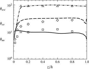
Figure 8 shows the variation of the inclination angles, ${\it\theta}_{uu}$ , ${\it\theta}_{vv}$ and ${\it\theta}_{ww}$ , as a function of the distance from the wall, from the nested-LES results at $1000\leqslant Re_{{\it\tau}}\leqslant 10\,000$ , compared to the inclination angles reported from DNS of turbulent channel flow at $Re_{{\it\tau}}\approx 950$ (del Alamo et al. Reference del Alamo, Jimenez, Zandonade and Moser2004; Sillero et al. Reference Sillero, Jimenez and Moser2014). In the channel core, the inclination angles predicted by nested-LES asymptote to values of 10°, 25° and 90° for ${\it\theta}_{uu}$ , ${\it\theta}_{vv}$ , and ${\it\theta}_{ww}$ , respectively, which agree reasonably well with the inclination angles reported by Sillero et al. (Reference Sillero, Jimenez and Moser2014) in DNS of turbulent channel flow at $Re_{{\it\tau}}\approx 950$ . The discrepancies observed in figure 8 can be attributed to the different methodologies used for obtaining the inclination angles in the present study compared to Sillero et al. (Reference Sillero, Jimenez and Moser2014).

Figure 8.

Inclination angles predicted by nested-LES in equilibrium turbulent channel flow at $1000\leqslant Re_{{\it\tau}}\leqslant 10\,000$ , compared to DNS results at $Re_{{\it\tau}}\approx 950$ (del Alamo et al. Reference del Alamo, Jimenez, Zandonade and Moser2004; Sillero et al. Reference Sillero, Jimenez and Moser2014). ▫, ♢, ▵, inclination angles ${\it\theta}_{uu}$ , ${\it\theta}_{vv}$ , ${\it\theta}_{ww}$ , respectively, predicted by nested-LES; ——, – – –, – $\,\cdot \,$ –, inclination angles, ${\it\theta}_{uu}$ , ${\it\theta}_{vv}$ , ${\it\theta}_{ww}$ , respectively, predicted by DNS.

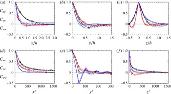
Figure 9 shows the 1-D two-point correlation functions predicted by nested-LES for all components of the velocity fluctuations in the outer layer ( $z/h\approx 0.5$ ) and the near-wall region ( $z^{+}\approx 10$ ). The 1-D two-point correlations at $z^{+}\approx 10$ were computed from the minimal flow unit of nested-LES, and show evidence of the presence of a streaky structure with a streak spacing of ${\sim}100$ wall units in the near-wall region in (figure 9 e). This indicates that the near-wall dynamics is adequately captured by nested-LES. As with all LES, the diameter of the near-wall streamwise vortices is overpredicted by nested-LES in (figure 9 e), because the grid spacing of ${\it\Delta}_{y}^{+}\approx 25$ –30, employed in the minimal flow unit of nested-LES, is of the same order as the diameter of these structures.

Figure 9.

Two-point correlations predicted by nested-LES in equilibrium turbulent channel flow at $1000\leqslant Re_{{\it\tau}}\leqslant 10\,000$ in (a–c) the outer region ( $z/h\approx 0.5$ ), obtained from the full domain; (d–f) the near-wall region ( $z^{+}\approx 10$ ), obtained from the minimal flow unit. Black lines with ▫, $C_{uu}$ ; red lines with ♢, $C_{vv}$ ; blue lines with ▵, $C_{ww}$ ; line types as in figure 4.

From the two-point correlation functions, one may obtain a measure of the average size of the structures by computing the integral length scales, ${\it\Lambda}_{{\it\alpha},{\it\varphi}}$ , given by

(4.3) $$\begin{eqnarray}{\it\Lambda}_{{\it\alpha},{\it\varphi}}=\int C_{{\it\varphi}{\it\varphi}}(\boldsymbol{r},\boldsymbol{r}^{\prime })\,\text{d}r_{{\it\alpha}},\end{eqnarray}$$

where $r_{{\it\alpha}}$ denotes $x$ , $y$ or $z$ . The integrals in (4.3) were computed only to $C_{{\it\varphi}{\it\varphi}}=0.05$ , to avoid the noisy correlation tails and long negative regions in $C_{{\it\varphi}{\it\varphi}}$ , which could cancel out the positively correlated regions (Sillero et al. Reference Sillero, Jimenez and Moser2014).

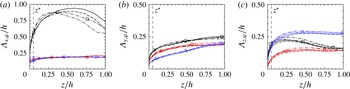
Figure 10 shows the integral length scales as a function of the wall-normal distance, from nested-LES at $1000\leqslant Re_{{\it\tau}}\leqslant 10\,000$ . The sizes of the structures, as inferred from ${\it\Lambda}_{{\it\alpha},{\it\varphi}}(z)$ , better motivate the construction of the grid and the choice of $z^{\ast }/h=0.05$ in the present study. From figure 10, it can be seen that for $z\geqslant z^{\ast }$ , the structures have a size ${\it\Lambda}_{x,{\it\varphi}}>0.15$ , ${\it\Lambda}_{y,{\it\varphi}}>0.07$ and ${\it\Lambda}_{z,{\it\varphi}}>0.07$ . Therefore, for $z>z^{\ast }$ , the grid spacings of ${\it\Delta}_{x}/h=0.1$ , ${\it\Delta}_{y}/h=0.05$ and ${\it\Delta}_{z}/h\approx 0.05$ , employed in the full domain of nested-LES in the present study, can adequately resolve these structures. However, for $z<z^{\ast }$ , ${\it\Lambda}_{x,v}/h$ and ${\it\Lambda}_{x,w}/h$ become comparable to ${\it\Delta}_{x}/h$ , while ${\it\Lambda}_{y,w}/h$ becomes smaller than ${\it\Delta}_{y}/h$ in the full domain. Thus the full domain can no longer properly resolve these structures, and the basis for renormalization of the velocity field in (2.2)–(2.4) needs to be switched from the full domain to the minimal flow unit.

Figure 10.

The integral scales, ${\it\Lambda}_{{\it\alpha},{\it\varphi}}$ , predicted by nested-LES in equilibrium turbulent channel flow at $1000\leqslant Re_{{\it\tau}}\leqslant 10\,000$ . Black lines with ▫, ${\it\Lambda}_{{\it\alpha},u}$ ; red lines with ♢, ${\it\Lambda}_{{\it\alpha},v}$ ; blue lines with ▵, ${\it\Lambda}_{{\it\alpha},w}$ ; line types as in figure 4.

The ${\it\Lambda}_{z,{\it\varphi}}$ of figure 10 also motivate the construction of the grid and the required number of grid points in the wall-normal direction. In the wake region ( $z/h>0.1$ ), the ${\it\Lambda}_{z,{\it\varphi}}$ nearly plateau and all ${\it\Lambda}_{z,{\it\varphi}}/h$ have values greater than 0.1. Consequently a fixed number of grid points with a nearly uniform grid of size ${\it\Delta}_{z}/h\approx 0.05{-}0.1$ can properly resolve the turbulence structures in this region at all Reynolds numbers. In contrast, for $z/h<0.1$ , the size of ${\it\Lambda}_{z,{\it\varphi}}$ grows approximately linearly with the distance from the wall, and $O(\log Re_{{\it\tau}})$ grid points are needed to resolve these structures, as shown in § 6.

4.5 Effect of $z^{\ast }$

We next examine the effect of placement of $z^{\ast }$ , the wall-normal location at which the basis for renormalization of the velocity field is switched from the velocity field in the minimal flow unit (for $z\leqslant z^{\ast }$ ) to the velocity field in the full domain (for $z>z^{\ast }$ ), on the predicted flow statistics and structure. To this end, nested-LES were performed at $Re_{{\it\tau}}\approx 2000$ with $z^{\ast }/h=0.025$ , 0.04, 0.07, 0.10, 0.15 and 0.20.

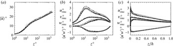
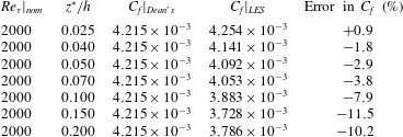
The results are summarized in table 4 and figure 11. The most accurate predictions of $C_{f}$ and the mean statistics are obtained with $z^{\ast }/h=0.04$ or 0.05. When $z^{\ast }/h$ is moved closer to the wall, the computations become under-resolved between $z^{\ast }/h<z/h<0.05$ because of the coarse grid spacings in the $x$ and $y$ directions in the full domain. When $z^{\ast }/h$ is moved above $z/h=0.05$ , the computations suffer from the inadequate size of the minimal flow unit in the region $0.05<z/h<z^{\ast }/h$ . It appears that the best results are obtained when the solution is switch from the minimal flow unit to the full domain as soon as the grid resolution in the full domain becomes adequate.

Figure 11.

Effect of $z^{\ast }/h$ on the profiles of the mean velocity, turbulence intensities, and Reynolds shear stress predicted by nested-LES in equilibrium turbulent channel flow at $Re_{{\it\tau}}\approx 2000$ . ${-}\,\cdot \cdot \,\,{-}$ ,  $z^{\ast }/h=0.025$ ; – – –, $z^{\ast }/h=0.04$ ; ——, $z^{\ast }/h=0.05$ ; – $\,\cdot \,$ –,  $z^{\ast }/h=0.07$ ; — $\,\cdot \cdot \,$ —,  $z^{\ast }/h=0.10$ ; — $\,\cdot \,$ —,  $z^{\ast }/h=0.15$ ; — —, $z^{\ast }/h=0.20$ ; ○, DNS at $Re_{{\it\tau}}\approx 2000$ (Hoyas & Jimenez Reference Hoyas and Jimenez2006).

Table 4.

The skin friction coefficient, $C_{f}$ , predicted in nested-LES of equilibrium turbulent channel flow at $Re_{{\it\tau}}\approx 2000$ with different locations of $z^{\ast }/h$ .

While choosing a non-optimal value of $z^{\ast }$ slightly degrades the performance of nested-LES, it is not catastrophic. The effect is even less prominent in the prediction of the flow structures, as shown in figure 12, where the streamwise and spanwise sections of two-point correlation coefficient, $C_{{\it\varphi}{\it\varphi}}$ , for all components of the velocity fluctuations at $z/h=0.1$ and $z/h=0.6$ , are plotted for nested-LES at $Re_{{\it\tau}}\approx 2000$ with $z^{\ast }/h=0.025$ , 0.04, 0.04 and 0.07. The contours of $C_{{\it\varphi}{\it\varphi}}$ predicted with different $z^{\ast }$ are seen to nearly collapse, with the exception of the large, weakly correlated structures for  $C_{uu}$ .

Figure 12.

Streamwise ( $xz$ ) (a,c,e,g,i,k), and spanwise ( $yz$ ) (b,d,f,h,j,l) sections of the correlation maps predicted by nested-LES in equilibrium turbulent channel flow at $Re_{{\it\tau}}\approx 2000$ with $z^{\ast }$ placed at $z^{\ast }/h=0.025$ , 0.04, 0.05, and 0.07: (a–f) $z/h=0.1$ , (g–l) $z/h=0.6$ ; (a,b,g,h) $C_{uu}$ ; (c,d,i,j) $C_{vv}$ ; (e,f,k,l) $C_{ww}$ . Line types as in figure 11; contour levels as in figure 7.

Figure 13.

(a,c,e,g) Time-averaged renormalization functions, $\langle R({\it\phi}_{{\it\alpha},\mathscr{D}})\rangle$ , and (b,d,f,h) deviations of $\langle R({\it\phi}_{{\it\alpha},\mathscr{D}})\rangle$ from unity, from nested-LES of equilibrium turbulent channel flow at (a,b) $Re_{{\it\tau}}\approx 1000$ , (c,d) $Re_{{\it\tau}}\approx 2000$ , (e,f) $Re_{{\it\tau}}\approx 5000$ , (g,h) $Re_{{\it\tau}}\approx 10\,000$ : ○, $R(\langle \langle \overline{u}_{\mathscr{D}}\rangle \rangle \langle \langle \overline{u}_{\mathscr{D}}\rangle \rangle )$ ; ▫, $R(\langle \langle \overline{u}_{\mathscr{D}}^{\prime \prime }\overline{u}_{\mathscr{D}}^{\prime \prime }\rangle \rangle )$ ; ♢, $R(\langle \langle \overline{v}_{\mathscr{D}}^{\prime \prime }\overline{v}_{\mathscr{D}}^{\prime \prime }\rangle \rangle )$ ; ▵, $R(\langle \langle \overline{w}_{\mathscr{D}}^{\prime \prime }\overline{w}_{\mathscr{D}}^{\prime \prime }\rangle \rangle )$ ; the error bars in (a,c,e,g) show $\pm$ one standard deviation in time.

4.6 Renormalization functions

The ability of nested-LES to accurately predict the turbulence statistics, structures and spectra results from only minor renormalizations of the velocity fields in the full domain and minimal flow unit at each time step during the course of the simulation. Figure 13 shows the profiles of the time-averaged renormalization functions, $\langle R({\it\phi}_{{\it\alpha},\mathscr{D}})\rangle$ , along with the absolute magnitudes of $|1-\langle R({\it\phi}_{{\it\alpha},\mathscr{D}})\rangle |$ , from nested-LES of turbulent channel flow at $1000\leqslant Re_{{\it\tau}}\leqslant 10\,000$ . In all cases, the time-averaged renormalization functions, $\langle R({\it\phi}_{{\it\alpha},\mathscr{D}})\rangle$ , remain close to unity and stay confined to $1\pm 0.025$ for $0\leqslant z/h<0.02$ ; $1\pm 0.005$ for $0.02\leqslant z/h<0.05$ ; and $1\pm 0.001$ for $0.05\leqslant z/h\leqslant 1$ . The main effect of $R({\it\phi}_{{\it\alpha},\mathscr{D}})$ in the inner layer ( $z\leqslant z^{\ast }$ ) is to enhance the wall-normal turbulence intensities in the full domain by 0.1–2.5 %, while attenuating the spanwise turbulence intensities by 0.1–2.5 % on average at each time step. In addition, the streamwise turbulence intensities and the mean streamwise velocity are attenuated in the inner layer of the full domain by 0.05–0.5 % on average at each time step. In the outer layer ( $z>z^{\ast }$ ), the main effect of $R({\it\phi}_{{\it\alpha},\mathscr{D}})$ is to attenuate the wall-normal turbulence intensities in the minimal flow unit by less than 0.1 %, while enhancing the streamwise and spanwise turbulence intensities by less than 0.1 % and the streamwise mean velocity by less than 0.05 % on average at each time step. These small corrections, when applied at every time step, are sufficient to correct the velocity fields, spectra and turbulence statistics in both the full domain and minimal flow unit of the nested-LES approach.

Figure 14 shows the time histories of the instantaneous renormalization functions, $R(\langle \langle \overline{u}_{{\it\alpha},\mathscr{D}}\rangle \rangle \langle \langle \overline{u}_{{\it\alpha},\mathscr{D}}\rangle \rangle )$ and $R(\langle \langle \overline{u}_{{\it\alpha},\mathscr{D}}^{\prime \prime }\overline{u}_{{\it\alpha},\mathscr{D}}^{\prime \prime }\rangle \rangle )$ , for the ‘mean’ and fluctuating components of the velocity, respectively, from nested-LES of turbulent channel flow at $Re_{{\it\tau}}\approx 10\,000$ . Similar features are observed at other Reynolds numbers. At all Reynolds numbers, $R({\it\phi}_{{\it\alpha},\mathscr{D}})$ remain close to unity for $z/h\geqslant 0.05$ , while fluctuating within $1\pm 0.01$ for $R(\langle \langle \overline{u}_{\mathscr{D}}\rangle \rangle \langle \langle \overline{u}_{\mathscr{D}}\rangle \rangle )$ and $R(\langle \langle \overline{u}_{\mathscr{D}}^{\prime \prime }\overline{u}_{\mathscr{D}}^{\prime \prime }\rangle \rangle )$ , and within $1\pm 0.03$ for $R(\langle \langle \overline{v}_{\mathscr{D}}^{\prime \prime }\overline{v}_{\mathscr{D}}^{\prime \prime }\rangle \rangle )$ and $R(\langle \langle \overline{w}_{\mathscr{D}}^{\prime \prime }\overline{w}_{\mathscr{D}}^{\prime \prime }\rangle \rangle )$ for $z/h<0.05$ , with the maximum variations occurring close to the wall. When the nested-LES is started from the initial velocity field, the renormalization functions quickly converge to the range above, and no clipping or damping is needed to maintain the stability of the simulations. During the course of the simulations, the values of $R({\it\phi}_{{\it\alpha},\mathscr{D}})$ at a given $z$ -location occasionally cross unity, meaning that a given component of velocity at a given location can alternate between being instantaneously amplified or attenuated. The variations in the renormalization functions with time reflect the deviations of the single-time statistics, used in the decomposition and renormalization procedures of nested-LES, from converged statistics. The moderate level of time variations in the renormalization functions indicates the presence of some level of statistical convergence in the single-time ensembles used in the decomposition and renormalization procedures of nested-LES, while not overwhelming the instantaneous dynamics of turbulence.

Figure 14.

Time history of the instantaneous renormalization functions, $R({\it\phi}_{{\it\alpha},\mathscr{D}})$ , at wall-normal locations $10^{-3}\leqslant z/h\leqslant 1.0$ , from nested-LES of equilibrium turbulent channel flow at $Re_{{\it\tau}}\approx 10\,000$ . (a) $R(\langle \langle \overline{u}_{\mathscr{D}}\rangle \rangle \langle \langle \overline{u}_{\mathscr{D}}\rangle \rangle )$ , (b) $R(\langle \langle \overline{u}_{\mathscr{D}}^{\prime \prime }\overline{u}_{\mathscr{D}}^{\prime \prime }\rangle \rangle )$ , (c) $R(\langle \langle \overline{v}_{\mathscr{D}}^{\prime \prime }\overline{v}_{\mathscr{D}}^{\prime }\rangle \rangle )$ , (d) $R(\langle \langle \overline{w}_{\mathscr{D}}^{\prime \prime }\overline{w}_{\mathscr{D}}^{\prime \prime }\rangle \rangle )$ .

4.7 Comparison to non-nested LES

To better understand the mechanisms behind the performance of the nested-LES approach, the simulations at $Re_{{\it\tau}}\approx 2000$ were repeated as non-nested LES in channels with the same domain sizes and grid resolutions as those employed in the full domain and minimal flow unit of nested-LES. These cases are denoted by $2000^{F}$ and $2000^{M}$ in tables 1 and 3.

The skin friction coefficients predicted in these non-nested LES cases had errors of 31.2 % and 21.6 %, for cases $2000^{F}$ and $2000^{M}$ , respectively, compared to Dean’s correlation, as shown in table 3. These errors should be contrasted with the error of 2.9 % in the prediction of $C_{f}$ by nested-LES approach at the same Reynolds number, with the same domain sizes and grid spacings. The source of the large errors in $C_{f}$ for case $2000^{F}$ is lack of adequate resolution in the near-wall region, while for case $2000^{M}$ , the large errors in $C_{f}$ arise from the lack of adequate domain size in the outer layer. These errors point to the need for two-way coupling in nested-LES. Clearly, the errors in $C_{f}$ of non-nested cases can be reduced by performing well-resolved non-nested, conventional LES in the full-size domain, as shown by the case $2000^{F,h}$ in table 3. But such computations require $O(256^{3})$ grid points compared to $O(64^{3})$ of nested-LES.

The one-point turbulence statistics predicted by these non-nested LES cases also show poor agreement with DNS and resolved conventional LES, as shown in figure 15. For case $2000^{F}$ , the mean velocity profile is overpredicted throughout the cross-section of the channel and there is significant pileup of the turbulence kinetic energy near the peaks of the streamwise and spanwise turbulence intensities, which is accompanied by underprediction of the wall-normal turbulence intensity. This pileup of streamwise turbulence kinetic energy can be attributed to the lack of adequate grid resolution in case $2000^{F}$ in the inner layer, needed to resolve the pressure–strain correlations, which are responsible for redistribution of the turbulence kinetic energy from the streamwise to cross-stream directions. For case $2000^{M}$ , the mean velocity profile exhibits an upward shift of the logarithmic layer and an excessive wake region. At the same time, the peak of the streamwise turbulence intensity is overpredicted in the inner layer, and the turbulence intensities are excessively isotropic in the outer layer. The latter feature is caused by the minimal size of the computational domain, which prevents the large scales from developing into their natural anisotropic states. All these problems are resolved when the nested-LES approach is used. Figure 15 shows the turbulence statistics obtained from both the full domain and minimal flow unit of nested-LES. The differences between the two sets of turbulence statistics are hardly noticeable, reflecting the near unity values of $R({\it\phi}_{{\it\alpha},\mathscr{D}})$ in (2.4).

Figure 15.

Profiles of the mean velocity, turbulence intensities and Reynolds shear stress predicted by nested-LES and non-nested LES in equilibrium turbulent channel flow at $Re_{{\it\tau}}\approx 2000$ ;  

, full domain of nested-LES (case 2000);   

, minimal flow unit of nested-LES (case 2000); — —, non-nested LES in full domain (case $2000^{F}$ ); — $\,\cdot \,$ —, non-nested LES in minimal flow unit (case $2000^{M}$ );  

 (orange), resolved conventional LES in full domain (case $2000^{F,h}$ ); ○, DNS at $Re_{{\it\tau}}\approx 2000$ (Hoyas & Jimenez Reference Hoyas and Jimenez2006).

Figure 16.

One-dimensional energy spectra of the streamwise ( $E_{uu}$ ), spanwise ( $E_{vv}$ ) and wall-normal ( $E_{ww}$ ) velocity fluctuations, predicted by nested-LES and non-nested LES in equilibrium turbulent channel flow at $Re_{{\it\tau}}\approx 2000$ in (a,b) outer region ( $z/h\approx 0.5$ ), (c,d) near-wall region ( $z^{+}\approx 20$ ): (a,c), energy spectra in the streamwise direction; (b,d), energy spectra in the spanwise direction.  

 (black, thick lines),  

 (dark red, thick lines),  

 (dark blue, thick lines):  $E_{uu}$ , $E_{vv}$ , $E_{ww}$ , respectively, from full domain of nested-LES (case 2000);   

 (black, thin lines),   

 (dark red, thin lines),   

 (dark blue, thin lines):  $E_{uu}$ , $E_{vv}$ , $E_{ww}$ , respectively, from minimal flow unit of nested-LES (case 2000);  

 (grey, thick lines),  

 (light red, thick lines),  

 (light blue, thick lines):  $E_{uu}$ , $E_{vv}$ , $E_{ww}$ , respectively, from non-nested LES in full domain (case $2000^{F}$ ); — — (grey, thin lines), — $\,\cdot \,$ — (light red, thin lines), — $\,\cdot \cdot \,$ — (light blue, thin lines): $E_{uu}$ , $E_{vv}$ , $E_{ww}$ , respectively, from non-nested LES in minimal flow unit (case $2000^{M}$ ); ▫ (black), ♢ (red), ▵ (blue), $E_{uu}$ , $E_{vv}$ , $E_{ww}$ , respectively, from DNS at $Re_{{\it\tau}}\approx 2000$ (Hoyas & Jimenez Reference Hoyas and Jimenez2006).

The key to the performance of the nested-LES approach can be understood by comparing the kinetic energy spectra obtained from nested-LES at $Re_{{\it\tau}}\approx 2000$ to the non-nested LES cases of $2000^{F}$ and $2000^{M}$ . Figure 16 shows the normalized 1-D energy spectra of the components of the fluctuating velocity in these simulations in the outer layer ( $z/h\approx 0.5$ ) and the near-wall region ( $z^{+}\approx 20$ ), compared to the DNS data of Hoyas & Jimenez (Reference Hoyas and Jimenez2006). In the outer layer (figure 16 a,b), both the full domain of nested-LES and the non-nested LES case of $2000^{F}$ predict spectra in good agreement with DNS, with nested-LES showing slightly better agreement with DNS than case $2000^{F}$ . The good agreement between the spectra from case $2000^{F}$ and DNS in the outer layer justifies using the full-domain solution as the basis of renormalization of the velocity field in the outer layer in the nested-LES approach. The non-nested LES case of $2000^{M}$ , however, predicts spectra in the outer layer which are in poor agreement with DNS. The minimal size of the domain, in this case, is not sufficient to accommodate the large-scale structures in the outer layer, and results in spectra for case $2000^{M}$ which prematurely approach the large-scale behaviour and become ‘flat’ in the inertial range. The two-way coupling between the minimal flow unit and the full domain in nested-LES alleviates these problems, and brings the spectra in the large scales of the minimal flow unit of nested-LES closer to inertial range behaviour and DNS results. In the formulation of nested-LES, only the ‘magnitudes’ of the kinetic energies of the components of turbulent velocity fluctuations are rescaled at each wall-normal location, without any explicit modifications to the spectral distributions of the kinetic energies in the wall-parallel directions. Nonetheless, in practice, the renormalization procedure also corrects the ‘shape’ of the spectra during the course of the simulation, thus restoring both the large-scale anisotropy in the outer layer of the minimal flow unit based on results from the full domain of nested-LES, and correcting the energy cascade in the outer layer of the minimal flow unit.

Similarly, in the near-wall region (figure 16 c,d), both the minimal flow unit of nested-LES and the non-nested LES case of $2000^{M}$ predict spectra in agreement with DNS. This justifies using the LES solution from the minimal flow unit as the basis of renormalization of the velocity field in the inner layer in the nested-LES approach. The non-nested LES case of $2000^{F}$ , however, predicts spectra which are in poor agreement with DNS in the near-wall region. The spectra of the streamwise and spanwise velocity fluctuations are overpredicted, while those of the wall-normal velocity fluctuations are underpredicted, for case $2000^{F}$ , consistent with the trends observed in the turbulence intensities in figure 15(b). The renormalization procedure in nested-LES alleviates these problems, and brings both the magnitudes and distributions of the full-domain spectra of nested-LES in closer agreement to DNS results in the inner layer. The renormalization procedure in this case, in essence, compensates for the under-resolved pressure–strain correlations in the coarse-resolution full domain, thus correcting the full-domain solution of nested-LES in the inner layer.

5.1 Evolution of the skin friction coefficient

Figure 17(a,b) show the evolution of the streamwise and spanwise skin friction coefficients, $C_{f,x}$ and $C_{f,y}$ , predicted in nested-LES, compared to experimental measurements of Driver & Hebbar (Reference Driver and Hebbar1991). In the straining zone, the $C_{f,x}$ predicted by nested-LES experiences an initial drop of ${\approx}20\,\%$ from its value in the base equilibrium flow, followed by recovery to a value ${\approx}20\,\%$ higher than that in the base equilibrium flow, while $C_{f,y}$ rapidly settles to a magnitude comparable to $C_{f,x}$ . While no experimental measurements of $C_{f,x}$ and $C_{f,y}$ are available in the straining zone, the features observed in nested-LES are similar to those reported in previous DNS studies of strained turbulent channel flow (Coleman, Kim & Le Reference Coleman, Kim and Le1996), and LES of 3-D shear-driven TBL flow (Kannepalli & Piomelli Reference Kannepalli and Piomelli2000) at lower Reynolds numbers.

Figure 17.

Evolution of (a) streamwise skin friction coefficient, $C_{f,x}$ , (b) spanwise skin friction coefficient, $C_{f,y}$ , (c) surface-flow angle, ${\it\beta}$ , predicted by nested-LES and non-nested LES in non-equilibrium, strained turbulent channel flow, compared to experiments (Driver & Hebbar Reference Driver and Hebbar1991). ——, nested-LES, case 2000- $S$ ; – – –, non-nested LES, case 2000- $S^{F}$ ; – $\,\cdot \,$ –, non-nested LES, case 2000- $S^{M}$ ; ○, experiments of Driver & Hebbar (Reference Driver and Hebbar1991).

In the recovery zone, the $C_{f,x}$ predicted by nested-LES experiences a rapid drop of ${\approx}10\,\%$ for $0\leqslant x^{\ast }\lesssim 0.5$ , followed by more gradual decay towards its base equilibrium channel value, while $C_{f,y}$ exhibits an exponential decay towards zero. Good overall agreement is observed between the $C_{f,x}$ and $C_{f,y}$ predicted by nested-LES and experimental data. However, the initial rapid drop of $C_{f,x}$ in the recovery region predicted by nested-LES occurs faster than experiments. This difference can be attributed to the more abrupt cessation of the transverse motion of the wall in the simulations compared to experiments.

Figure 18.

Profiles of the mean velocities and turbulent stresses at $x^{\ast }\approx -0.11$ , near the end of the straining zone, predicted by nested-LES and non-nested LES in shear driven, strained turbulent channel flow, compared to experimental measurements in shear driven, three-dimensional TBL (Driver & Hebbar Reference Driver and Hebbar1991). ——, nested-LES, case 2000- $S$ ; – – –, non-nested LES, case 2000- $S^{F}$ ; – $\,\cdot \,$ –, non-nested LES, case 2000- $S^{M}$ ; $\cdots \cdots$ , nested-LES in equilibrium turbulent channel flow at $Re_{{\it\tau}}\approx 2000$ ; ○, experimental data of Driver & Hebbar (Reference Driver and Hebbar1991). An enlarged view of the near-wall region is shown below each figure.

In contrast, the non-nested LES case of 2000- $S^{F}$ exhibits significant lag in response to both the impulsive start and cessation of straining, and significantly underpredicts the magnitudes of $C_{f,x}$ and $C_{f,y}$ . The non-nested LES case of 2000- $S^{M}$ predicts the evolution of $C_{f,x}$ and $C_{f,y}$ with features similar to those in nested-LES, but underpredicts the $C_{f,x}$ and $C_{f,y}$ by 10–15 %.

Figure 17(c) shows the evolution of the surface flow angle on the moving wall, defined as ${\it\beta}\equiv \tan ^{-1}(C_{f,y}/C_{f,x})$ . Nearly identical surface flow angles are predicted by nested-LES and non-nested LES cases of 2000- $S^{F}$ and 2000- $S^{M}$ , all showing good agreement with experimental data in the recovery zone. The largest discrepancies from experiments are seen for case 2000- $S^{F}$ .

5.2 Evolution of one-point turbulence statistics

Figure 18 shows the profiles of the mean velocities and turbulent stresses predicted by the simulations, compared to experiments (Driver & Hebbar Reference Driver and Hebbar1991), at $x^{\ast }\approx -0.11$ , near the end of the straining zone. The mean spanwise velocity, $\langle \overline{v}\rangle$ , develops a profile which approximately satisfies $\langle \overline{v}\rangle /V_{s}=1-\langle \overline{u}\rangle /U_{\infty }$ , as shown in figure 19. The presence of this mean spanwise velocity leads to significant enhancement of all components of turbulent stresses in the strained flow compared to the base equilibrium flow, while the reorientation of the flow gives rise to non-zero Reynolds stresses $\langle u^{\prime }v^{\prime }\rangle$ and $\langle v^{\prime }w^{\prime }\rangle$ , as seen in figure 18(c–h). All these predictions of nested-LES in the straining zone are in agreement with experimental data. The biggest discrepancy between experiments and nested-LES results is observed in the profile of $\langle v^{\prime }w^{\prime }\rangle$ at $x^{\ast }\approx -0.11$ (figure 18 h), where experimental data show features which are characteristic of the recovery zone, $x^{\ast }\geqslant 0$ . In contrast, the non-nested LES case of 2000- $S^{F}$ gives inaccurate predictions for all turbulent stresses as well as the mean spanwise velocity in both the inner and outer layers, while the non-nested LES case of 2000- $S^{M}$ gives acceptable results in the inner layer but predicts inaccurate turbulent stresses in the outer layer.

Figure 19.

Hodograph of the mean streamwise and spanwise velocities at $x^{\ast }\approx -0.11$ , near the end of the straining zone, predicted by nested-LES and non-nested LES, compared to experiments (Driver & Hebbar Reference Driver and Hebbar1991). ——, nested-LES, case 2000- $S$ ; – – –, non-nested LES, case 2000- $S^{F}$ ; – $\,\cdot \,$ –, non-nested LES, case 2000- $S^{M}$ ; ○, experiments of Driver & Hebbar (Reference Driver and Hebbar1991);  $\cdot \cdots$ , analytical expression $\langle \overline{u}\rangle /U_{\infty }+\langle \overline{v}\rangle /V_{s}=1$ .

Figure 20(a–h) show the evolution of the profiles of mean velocities and turbulent stresses predicted by nested-LES at $x^{\ast }\approx 0.23$ , in the initial recovery zone. In this zone, the effect of the abrupt cessation of the transverse motion of the wall remains confined to the near-wall region, and is most dramatically felt in the spanwise component of the velocity. Both $\langle \overline{v}\rangle$ and $\langle v^{\prime }v^{\prime }\rangle$ rapidly decay during this phase, while $\langle v^{\prime }w^{\prime }\rangle$ and $\langle u^{\prime }v^{\prime }\rangle$ develop negative peaks in the immediate vicinity of the wall. Interestingly, the near-wall peak of $\langle u^{\prime }u^{\prime }\rangle$ drops to 70 % of its value in the base equilibrium flow before recovery, which has also been observed in earlier numerical studies (Coleman et al. Reference Coleman, Kim and Le1996; Kannepalli & Piomelli Reference Kannepalli and Piomelli2000). The nested-LES approach successfully captures all these features in agreement with experimental data. In contrast, the non-nested LES case of 2000- $S^{F}$ exhibits significant lag in response to cessation of the transverse strain and fails to correctly predict any of the turbulent stresses or the mean spanwise velocity, while the non-nested LES case of 2000- $S^{M}$ predicts the turbulent stresses inaccurately in the outer layer.

Figure 20.

Profiles of the mean velocities and turbulent stresses predicted by nested-LES and non-nested LES in shear driven, strained turbulent channel flow, compared to experimental measurements in shear driven, three-dimensional TBL (Driver & Hebbar Reference Driver and Hebbar1991) in (a–h) the initial recovery zone, $x^{\ast }\approx 0.23$ , (i–p) the mid-recovery zone, $x^{\ast }\approx 0.91$ , (q–x) final recovery zone, $x^{\ast }\approx 10.9$ . Symbols and line types as in figure 18.

Figure 20(i–p) show the evolution of the profiles of the mean velocities and turbulent stresses predicted by nested-LES at $x^{\ast }\approx 0.9$ , in the mid-recovery zone. In this zone, the effect of cessation of straining begins to penetrate into the outer layer, and the profiles of all components of the Reynolds stresses continue to decay or recover towards their equilibrium states. The nested-LES approach successfully captures the flow features in this mid-recovery zone in agreement with experimental data. The biggest discrepancy is observed in the profiles of $\langle w^{\prime }w^{\prime }\rangle$ and $\langle v^{\prime }w^{\prime }\rangle$ , for which nested-LES predicts a faster decay compared to experiments. These discrepancies may be attributed to the larger spanwise and wall-normal turbulence intensities in the outer layer of TBL compared to channel flow (Jimenez et al. Reference Jimenez, Hoyas, Simens and Mizuno2010).

Figure 20(q–x) show the evolution of the profiles of the mean velocities and turbulent stresses predicted by nested-LES at $x^{\ast }\approx 10.9$ , in the final recovery zone. In this zone, all turbulence statistics are approaching their equilibrium states and the predictions of nested-LES show good agreement with experimental data, except for the discrepancy in the recovery of $\langle w^{\prime }w^{\prime }\rangle$ , $\langle v^{\prime }w^{\prime }\rangle$ , and $\langle u^{\prime }w^{\prime }\rangle$ in the outer layer, which can be attributed to the same reason noted before in the mid-recovery zone.

5.3 Renormalization functions

Figure 21 shows the profiles of the time-averaged renormalization functions, $\langle R({\it\phi}_{{\it\alpha},\mathscr{D}})\rangle$ , and the deviations of $\langle R({\it\phi}_{{\it\alpha},\mathscr{D}})\rangle$ from unity, $|1-\langle R({\it\phi}_{{\it\alpha},\mathscr{D}})\rangle |$ , observed in nested-LES of strained turbulent channel flow. Throughout the straining and recovery zones, the time-averaged renormalization functions, $\langle R({\it\phi}_{{\it\alpha},\mathscr{D}})\rangle$ , remain confined to $1\pm 0.03$ for $0\leqslant z/h<0.05$ , and $1\pm 0.001$ for $0.05\leqslant z/h\leqslant 1$ . In the recovery zone (figure 21 c,d), the trends in $\langle R({\it\phi}_{{\it\alpha},\mathscr{D}})\rangle$ remain close to those observed in equilibrium turbulent channel, except that $R(\langle \langle \overline{v}_{\mathscr{D}}^{\prime \prime }\overline{v}_{\mathscr{D}}^{\prime \prime }\rangle \rangle )$ is closer to unity in the near-wall region and has less fluctuation. In the straining zone (figure 21 a,b), the renormalization functions act to enhance the turbulence kinetic energy of $\langle \langle \overline{v}_{\mathscr{D}}\rangle \rangle$ and $\overline{v}_{\mathscr{D}}^{\prime \prime }$ by up to 0.5 % and 2 %, respectively, as required by the flow, instead of attenuating them, demonstrating the robustness of the nested-LES approach and its ability to adjust to different flow conditions.

Figure 21.

(a,c) Time-averaged renormalization functions, $\langle R({\it\phi}_{{\it\alpha},\mathscr{D}})\rangle$ , and (b,d) deviations of $\langle R({\it\phi}_{{\it\alpha},\mathscr{D}})\rangle$ from unity, from nested-LES of non-equilibrium, strained turbulent channel flow in (a,b) the straining zone, and (c,d) the recovery zone: ▿, $R(\langle \langle \overline{v}_{\mathscr{D}}\rangle \rangle \langle \langle \overline{v}_{\mathscr{D}}\rangle \rangle )$ ; other symbols as in figure 13.