


INTRODUCTION
Parasites are ubiquitous in nature, and have diverse life histories, transmission modes and ranges of host specificity (Poulin, Reference Poulin2011). Determining which host species a parasite can infect (referred to herein as the permissive host set or host range) could enable targeted host surveillance (Pilosof et al. Reference Pilosof, Morand, Krasnov and Nunn2015; Walton et al. Reference Walton, Marion, Davidson, White, Smith, Gavier-Widen, Yon, Hannant and Hutchings2016), estimation of zoonotic risk potential (Han et al. Reference Han, Schmidt, Bowden and Drake2015) and insight into parasite specialization/generalism (Poulin, Reference Poulin2005). However, host–parasite interactions are complex, and may be influenced by environment (Locke et al. Reference Locke, McLaughlin and Marcogliese2013), geography (Davies and Pedersen, Reference Davies and Pedersen2008), coevolutionary history (Krasnov et al. Reference Krasnov, Fortuna, Mouillot, Khokhlova, Shenbrot and Poulin2012) or trait matching between host and parasite (Rohr et al. Reference Rohr, Naisbit, Mazza and Bersier2016). The relative importance of these constraints is generally not known, impeding prediction of currently undersampled or unknown host–parasite associations. Previous efforts to characterize parasite communities have largely focused on parasite richness (Ezenwa et al. Reference Ezenwa, Price, Altizer, Vitone and Cook2006), topological network measures (Krasnov et al. Reference Krasnov, Fortuna, Mouillot, Khokhlova, Shenbrot and Poulin2012; Canard et al. Reference Canard, Mouquet, Mouillot, Stanko, Miklisova and Gravel2014) and parasite community dissimilarity (Locke et al. Reference Locke, McLaughlin and Marcogliese2013). However, few studies have focused on predicting which host species a parasite will infect (i.e. the permissive host set). As a result, the ability to predict the identity of permissive hosts (i.e. those that may be infected; host range) for a given parasite is limited and poses an obstructive knowledge gap. The development of predictive models could forecast parasite spillover to humans (Daszak et al. Reference Daszak, Cunningham and Hyatt2000) or wildlife (Colautti et al. Reference Colautti, Ricciardi, Grigorovich and MacIsaac2004), and could provide an understanding of what factors underlie host–parasite associations.
One major barrier to the development of predictive models of the permissive host set is the low quality of data [but see Strona and Lafferty (Reference Strona and Lafferty2012a )], limited tools to access these data [but see Dallas (Reference Dallas2016)] and a lack of cross-validated, accurate and predictive models. For instance, the PaNic model (Strona and Lafferty, Reference Strona and Lafferty2012b ) attempts to predict suitable fish host species given userweighted constraints (e.g. host trait weights or geographic constraints). While valuable, this tool has a limited feature space (e.g. only five host traits used for prediction), and cannot validate predictions, so there is no way to determine predictive accuracy. In essence, previous researchers asked which host species might be suitable for a parasite (Strona and Lafferty, Reference Strona and Lafferty2012a ), whereas we explored the factors that determine host suitability for a given parasite mechanistically, creating cross-validated models capable of predicting both known and potential permissive host set. Specifically, the known permissive host set would correspond to predictive accuracy of trained models on data not used to train the model, and the potential permissive host set would correspond to model-predicted suitable hosts without an observed occurrence record.
We used a large database on helminth infections of fish hosts (Strona et al. Reference Strona, Palomares, Bailly, Galli and Lafferty2013) to develop predictive models of the permissive host set for a number of parasite species (n = 562), using data on host traits, host taxonomy, geographic variables and parasite community variables. We found that the permissive host community is most constrained by the existing parasite community (i.e. parasite community variables), and much less so by geographic variables, host traits or host taxonomy. This suggests that the parasite community of a host species contains more information for predicting host–parasite associations and the permissive host set of a given parasite than the traditional host-centred approach, which places emphasis on host traits and taxonomy.
METHODS
Fish and parasite data
A global database of fish–parasite associations [FishPest (Strona et al. Reference Strona, Palomares, Bailly, Galli and Lafferty2013)] was used, consisting of over 38 000 helminth parasite records from three phyla (Acanthocephala, Nematoda, Platyhelminthes), including examples from each major class of parasitic platyhelminthes (Cestoda, Monogenea, Trematoda). Our analyses focused on parasite species with at least 10 host occurrence records (n = 562). Though rare, duplicate host records did exist in the database, such that some parasites specialized on a small number of hosts (e.g. Bicotylophora trachinoti was only found on five Trachinotus species). Models were trained only on unique host–parasite combinations, which resulted in a range of specialist and generalist parasites with a variety of transmission modes, life histories and distributions.
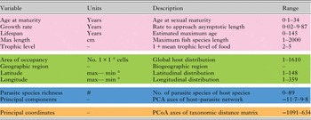
Fish trait and geographic data were obtained from FishPest (Strona and Lafferty, Reference Strona and Lafferty2012a ; Strona et al. Reference Strona, Palomares, Bailly, Galli and Lafferty2013) and FishBase (Froese and Pauly, Reference Froese and Pauly2000), a database of fish life history traits. Host trait variables included host age at sexual maturity, growth rate, lifespan, maximum body length and trophic level. Covariates relating to the geographic distribution of hosts included area of occupancy, biogeographic region (explained further in Supplemental Materials) and latitudinal/longitudinal range. Details of host trait and geographic variable determination are provided in Strona et al. (Reference Strona, Palomares, Bailly, Galli and Lafferty2013) and units are provided in Table 1. Missing covariate values were imputed through the iterative training of a machine learning algorithm (random forests), which imputes missing data based on averaged non-missing values weighted by proximity of observations in the random forest. This procedure was performed using the randomForest R package (Liaw and Wiener, Reference Liaw and Wiener2002). Parasite community variables were calculated using the first five principal components of the host–parasite interaction network, a binary matrix where host species are rows, parasite species are columns, and known interactions between host and parasite are denoted as 1. This approach captures parasite community structure by attempting to compress the information contained in the entire interaction matrix into a smaller set of explanatory vectors. Other approaches calculate summary statistics of the interaction matrix, such as parasite species richness of each host. We incorporate both approaches, using both principal components and parasite richness per host species as covariates. Principal components were calculated using the princomp function, with the focal parasite removed so as not to introduce bias, meaning that each model used slightly different principal component vectors. The amount of variance explained by the first five principal component (PCA) vectors was not strongly influenced by this (σ = 0·0006). Reducing binary covariates to a small number of features is difficult, and five PCA vectors explained only a portion of the variation in parasite community composition (average variance explained = 27%). Additional PCA vectors explained little more variation in parasite community composition (see Supplemental Materials), so only the first five PCA vectors were used.
Host traits may not provide a complete representation of functional differences among hosts that could determine parasite occurrence. Meanwhile, host taxonomy may capture unmeasured host trait variation. To incorporate host taxonomy into our analyses, we calculated the pairwise taxonomic dissimilarity between all host species using the vegan package in R, and then performed a Principal Coordinates Analysis on the taxonomic dissimilarity matrix to obtain a reduced set of features containing information on taxonomic dissimilarity of fish hosts. This procedure attempts to compress information contained in the host taxonomic dissimilarity matrix into a set of host-level covariates. Measures of taxonomic distinctiveness calculate the mean taxonomic distance for a host species to all other species, while our approach better captures the variation within the taxonomic dissimilarity matrix. We used the first five vectors from this analysis, which explained 40·5% of total variation in the host taxonomic dissimilarity matrix, to represent host taxonomic relationships.
The absence of a recorded host–parasite interaction does not rule out the existence of an association. One approach to account for this, originally developed for species distribution modelling, is to sample ‘background’ interactions, which we define as a random set of possible hosts for a focal parasite. In species distribution modelling, this would include both observed (i.e. occurrences) and unobserved interactions (Elith et al. Reference Elith, Phillips, Hastie, Dudík, Chee and Yates2011) aimed at characterizing the distribution of predictor variables across space. However, since parasite occurrence data were so limited, and duplicating hosts in the training data could introduce bias to our models, we sampled background data from the subset of host species where the focal parasite was not observed. Background data consisted of a random sample of 20 times the number of recorded parasite occurrences, which maintained a constant proportion of parasite presence values to background points. The use of background data is essential for model development, since the background sample represent the plausible ranges of host covariates (see Table 1), creating a parameter space of host covariates. The number of background hosts considered did not influence model predictions (see Supplementary Materials). Together, our data consisted of parasite occurrence records, which included both known parasite occurrences and background data, and a set of host-level covariates (Table 1) with which to predict parasite occurrence. These data were split into training (70%) and test (30%) sets in order to reduce model overfitting, and to evaluate predictive model accuracy on independent data (i.e. the test set).
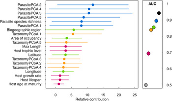
Relative contribution values (mean ± s.d.) from the full model (left panel; black point in right panel) demonstrate the importance of parasite community variables (blue) relative to host traits (pink), taxonomy (orange) and geographic covariates (green). Numbers following host taxonomic (TaxonomyPCoA) and parasite community (ParasitePCA) covariates refer to principal component axis number. Other variable definitions and units are available in Table 1. Accuracy of submodels (mean ± 2 × s.d.) trained on covariate groups (right panel) all performed better than a null expectation (grey point).

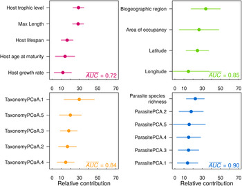
Relative importance (mean ± s.d.) and average model accuracy for each submodel trained on either host traits (top left), geographic covariates (top right), host taxonomic covariates (bottom left) or parasite community covariates (bottom right). Numbers following host taxonomic (TaxonomyPCoA) and parasite community (ParasitePCA) covariates refer to principal component axis number.


Predictive model formulation
Boosted regression trees (BRT), a powerful analysis that bypasses known issues with alternative regression analyses (Elith et al. Reference Elith, Leathwick and Hastie2008), were trained using R package gbm (Ridgeway, Reference Ridgeway2015) (learning rate = 0·001; interaction depth = 4). The optimal number of trees was determined using ‘out-of-bag’ estimation (max trees = 50 000). Boosting is a process where weak learning trees are built iteratively, and each tree is dependent on the residuals of the previous tree. This creates an ensemble of trees, which are then combined to create the final model. In our application, we trained models using geographic covariates, host traits, host taxonomy or parasite community covariates as a means to predict parasite occurrence on hosts in the independent test data.
Relative contribution (R c) values for each covariate were determined by permuting each predictor (i.e. randomizing to remove any potential influence on resulting model) and determining the resulting change in model performance. Some species could be found in many biogeographic regions, so binary dummy variables were used for this covariate, and the relative contribution value reported here is the sum of the relative contribution value for all binary dummy variables (see Supplementary Materials for further discussion). Accuracy was assessed using AUC (the area under the receiver operating characteristic curve), a measure scaled between 0 (perfectly inaccurate prediction) to 1 (perfect prediction), with a value of 0·5 corresponding to random prediction (Flach, Reference Flach, Sammut and Webb2010). Here, AUC measures the frequency with which a randomly sampled host species is parasitized would be more highly ranked by the BRT model than a randomly-selected host from the background data. A null model, representing the random prediction case discussed above, was used for comparison to trained models. Here, occurrences were randomly predicted, constrained by the total number of parasite occurrences in the test set (i.e. the number of parasite occurrences was kept constant).
RESULTS
All models performed better than null predictions (mean ± se; null model = 0·50 ± 0·0003). Trained models predicted the permissive host sets of parasite species with varying levels of accuracy (Fig. 1), depending on whether models were trained with data corresponding to host traits
 $(\overline {AUC} = 0 \!\cdot\! 69 \pm0 \!\cdot\! 007)$
, host taxonomic distinctiveness
 $(\overline {AUC} = 0 \!\cdot\! 84 \pm 0 \!\cdot\! 006)$
, geography
 $(\overline {AUC} = 0 \!\cdot\! 85 \pm 0 \!\cdot\! 005)$
, parasite community composition
 $(\overline {AUC} = 0 \!\cdot\! 90 \pm 0 \!\cdot\! 005)$
or all covariates
 $(\overline {AUC} = 0 \!\cdot\! 94 \pm 0 \!\cdot\! 003)$
.
The relative importance of covariates in submodels (models trained on only one covariate class) approximately retained their rank order position (Fig. 2) when compared with the full model (Fig. 1). Principal component (ParasitePCA) and principal coordinate (TaxonomyPCoA) axes change rank in submodels relative to the full model, likely because of the small difference in relative variable importance, and the broad overlap in error bars. This means that parasites responded differentially to PCA axes, suggesting that unique information is contained in each axis. Model performance did not differ by parasite taxonomic group (Supplementary Figure A2) or host specificity (Supplementary Figure A3).
DISCUSSION
Parasite community covariates were the most important variables to the full model, and had the highest submodel accuracy, despite the limited amount of variance explained by the decomposition of parasite community composition (i.e. the five PCA vectors). This suggests that parasite species cooccurrence data contain valuable information, either on unmeasured host trait variation, or on forces underlying parasite community composition among hosts (e.g. parasite competition, facilitation or community assembly). It is unlikely that the parasite community vectors could relate to unmeasured host trait variation, as the selected host traits have previously been related to parasite richness (Lindenfors et al. Reference Lindenfors, Nunn, Jones, Cunningham, Sechrest and Gittleman2007) and occurrence probability (Strona and Lafferty, Reference Strona and Lafferty2012b ). Further, unmeasured trait variation accounted for by parasite community covariates would have be entirely separate from other covariates (i.e. collinearity between unmeasured variation and measured host traits), which seems unlikely given known scaling relationships in host traits (Killen et al. Reference Killen, Atkinson and Glazier2010; Rall et al. Reference Rall, Brose, Hartvig, Kalinkat, Schwarzmüller, Vucic-Pestic and Petchey2012). On the other hand, if parasite community covariates were able to capture interactions among parasites, structural constraints to infection or the identity of coinfecting parasites, it is plausible to conclude that helminth parasites of fish form non-random, interacting communities. Whether this is the case or not, parasite community composition was key in predicting host community composition for a large number of parasites.
Previous studies have found host traits to be associated with parasite diversity (Locke et al. Reference Locke, Marcogliese and Valtonen2014) and parasite community similarity (Davies and Pedersen, Reference Davies and Pedersen2008). Further, host taxonomy and geography have been found to be associated with parasite occurrence probability (Strona et al. Reference Strona, Palomares, Bailly, Galli and Lafferty2013). Our findings do not disagree with these previous studies. Models trained using data on geographic covariates, host taxonomy and host traits still performed much better than our null model, suggesting that these groups of variables contain important information. Our findings do suggest, however, that parasite community structure may be more important than both host attributes and geography. We posit two hypotheses to explain why parasite community variables are important in predicting which hosts a given parasite infects. First, similar parasites may infect similar host species, resulting in the parasite community variables capturing parasite trait information. Second, parasites interact over long timescales, resulting in quantifiable non-random co-occurrence patterns capable of accurate host community prediction. The testing of these hypotheses is an undertaking that will require data on parasite traits and evolutionary histories, in conjunction with large databases of host–parasite interactions, such as the London Natural History Museum's helminth database (Gibson et al. Reference Gibson, Bray and Harris2005) and the Global Mammal Parasite Database (Nunn and Altizer, Reference Nunn and Altizer2005).
There is mixed evidence for the predictability of parasite community structure in fish parasites, despite the existence of an extensive body of literature on the subject (Holmes, Reference Holmes1990; Kennedy, Reference Kennedy, Esch, Bush and Aho1990, Reference Kennedy2009; Poulin and Rohde, Reference Poulin and Rohde1997; Sasal et al. Reference Sasal, Trouvé, Müller-Graf and Morand1999; Poulin and Valtonen, Reference Poulin and Valtonen2002; Rohde, Reference Rohde2002). As it is possible to predict the permissive host set using parasite community composition data, it may be possible to predict parasite community composition from the permissive host set. Further, given that parasite community composition was important, it is plausible that information on parasite traits, such as transmission mode, feeding behaviour or host tissue infected may increase the accuracy with which the permissive host set is determined. Interestingly, we found no difference in model accuracy as a function of parasite taxonomic group or number of hosts infected (see Supplementary Materials). This is intriguing, as it suggests that prediction of the host community (i.e. the permissive host set) may be possible even for specialized parasites or those with complex life histories. The application of our analytical approach to a broader range of host and parasite taxa, considering different spatial scales and incorporating information on more host and parasite traits may help discern when the permissive host set is predictable, and identify potential likely hosts for a given parasite species. Lastly, the compilation and curation of parasite trait databases, in the style of current host trait databases (Froese and Pauly, Reference Froese and Pauly2000), is necessary for the accurate forecasting of parasite occurrences on novel hosts.
SUPPLEMENTARY MATERIAL
The supplementary material for this article can be found at https://doi.org/10.1017/S0031182016001608. Data and R code to reproduce the analyses is provided at https://doi.org/10.6084/m9.figshare.3795330.
ACKNOWLEDGEMENTS
We thank Kevin Lafferty for providing comments on an earlier manuscript draft. The Macroecology of Infectious Disease Research Coordination Network (funded by NSF DEB 131223) provided useful discussions and support for this work.
FINANCIAL SUPPORT
T. A. D., A. W. P., and J. M. D. were supported by the Odum School of Ecology. T. A. D. is currently supported by the University of California at Davis.