1 Introduction
Frequently atmospheric or oceanic gravity currents propagate into stratified ambients, rather than into constant density environments. Density stratification due to gradients in temperature, moisture, salinity or sediment concentration, for example, may potentially result in significantly more complex dynamics of the flow, due to the formation of internal waves, with implications for the transport of nutrients or pollution (Rottman & Simpson Reference Rottman and Simpson1989; Maxworthy et al.
Reference Maxworthy, Leilich, Simpson and Meiburg2002; Nash & Moum Reference Nash and Moum2005; Kilcher & Nash Reference Kilcher and Nash2010). Within the current investigation, we will focus on the specific situation of a two-layer stratified ambient, with a density jump
 $\unicode[STIX]{x0394}\unicode[STIX]{x1D70C}$
between the lower and upper layers. For such flows we will formulate a group of models based on vorticity conservation arguments. Two-dimensional direct numerical simulation results will then be compared to predictions by these models, as well as to previous models developed by other authors.
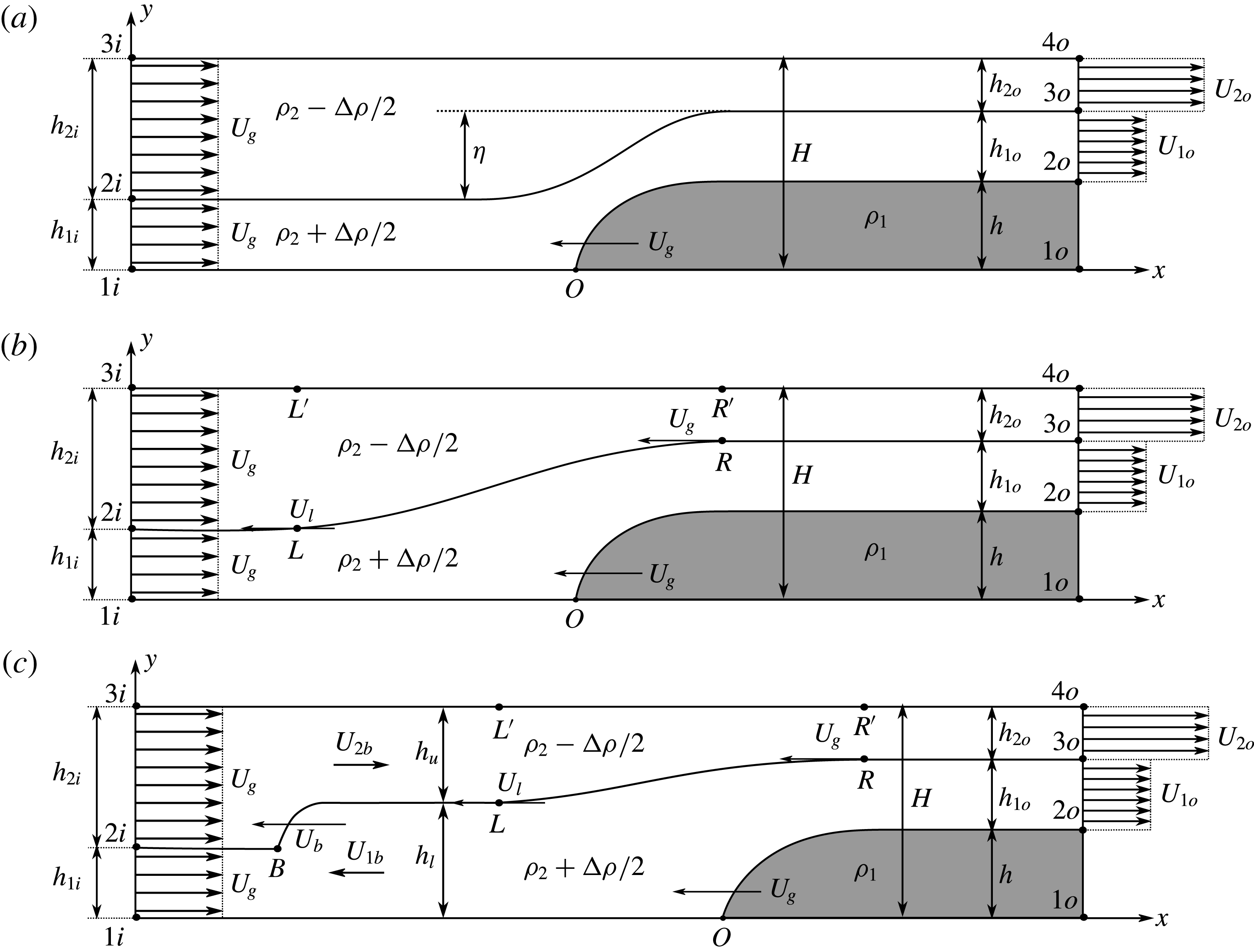
Schematic of a gravity current (shaded) propagating into a two-layer stratified ambient: (a) an upstream-propagating expansion wave does not form, (b) an upstream wave is generated that travels faster than the gravity current (
 $U_{l}>U_{g}$
) and (c) a hydraulic jump forms that propagates faster than both the upstream travelling wave and the gravity current (
 $U_{b}>U_{l}>U_{g}$
). The gravity current density
 $\unicode[STIX]{x1D70C}_{1}$
, the average ambient density
 $\unicode[STIX]{x1D70C}_{2}$
, the density jump
 $\unicode[STIX]{x0394}\unicode[STIX]{x1D70C}$
, the current height
 $h$
and the height
 $h_{1i}$
of the ambient interface at the inflow boundary are prescribed. Hereafter, configurations (a), (b) and (c) will be referred to as C1, C2 and C3, respectively.

Figure 1 presents a schematic of gravity currents propagating into two-layer stratified ambients. In the laboratory reference frame, the gravity current travels with a constant velocity
 $U_{g}$
from right to left, into quiescent fluid. For the sake of formulating simplified theoretical models, we shift into the reference frame of the gravity current. In this reference frame the gravity current is at rest, and the ambient fluid approaches from the left inflow boundary with
 $U_{g}$
. The gravity current density is denoted by
 $\unicode[STIX]{x1D70C}_{1}$
, while the two ambient layers have an average density of
 $\unicode[STIX]{x1D70C}_{2}$
, so that the densities of the upper and lower layers are
 $\unicode[STIX]{x1D70C}_{2}-\unicode[STIX]{x0394}\unicode[STIX]{x1D70C}/2$
and
 $\unicode[STIX]{x1D70C}_{2}+\unicode[STIX]{x0394}\unicode[STIX]{x1D70C}/2$
, respectively. We consider only bottom currents, so that
 $\unicode[STIX]{x1D70C}_{1}>\unicode[STIX]{x1D70C}_{2}+\unicode[STIX]{x0394}\unicode[STIX]{x1D70C}/2>\unicode[STIX]{x1D70C}_{2}-\unicode[STIX]{x0394}\unicode[STIX]{x1D70C}/2$
. Other flow parameters include the depths
 $h_{1i}$
and
 $h_{2i}$
of the ambient layers at the inlet, the gravity current height
 $h$
and the channel height
 $H$
.
The development of simplified theoretical models for configuration C1 in figure 1(a) dates back to the classical work by Holyer & Huppert (Reference Holyer and Huppert1980), who considered inviscid non-Boussinesq flows. They solve for both the height and the velocity of the gravity current, as functions of prescribed inflow layer depths and densities. The authors enforce mass conservation in each ambient layer, as well as the conservation of horizontal momentum for the entire channel. To obtain the pressure jump across the front, they assume hydrostatic pressure distributions in the uniform parallel flow regions far up- and downstream. They subsequently close their system of equations by employing Bernoulli’s equation along the stagnation point streamline
 $1i-O$
in figure 1(a), as well as along streamlines
 $O-2o$
and
 $2i-3o$
. Consequently, their model does not allow for energy dissipation in the ambient layers. As they observe multiple solutions for the gravity current height, the authors argue that nature prefers the solution that maximizes the volumetric inflow rate, which always corresponds to the largest gravity current height. The authors then extend their analysis to dissipative flows, by allowing for head losses in their respective Bernoulli equations. They proceed to calculate the rate of energy dissipation
 ${\dot{E}}_{d}$
for the entire flow, and accept the solution that maximizes
 ${\dot{E}}_{d}$
for a constant volumetric inflow rate. This model was subsequently modified by Crook (Reference Crook, Lilly and Gal-Chen1983), who considers non-dissipative flows in the Boussinesq limit with an upstream-propagating bore. The author assumes an infinitely deep channel, so that the velocity in the upper ambient layer is the same everywhere.
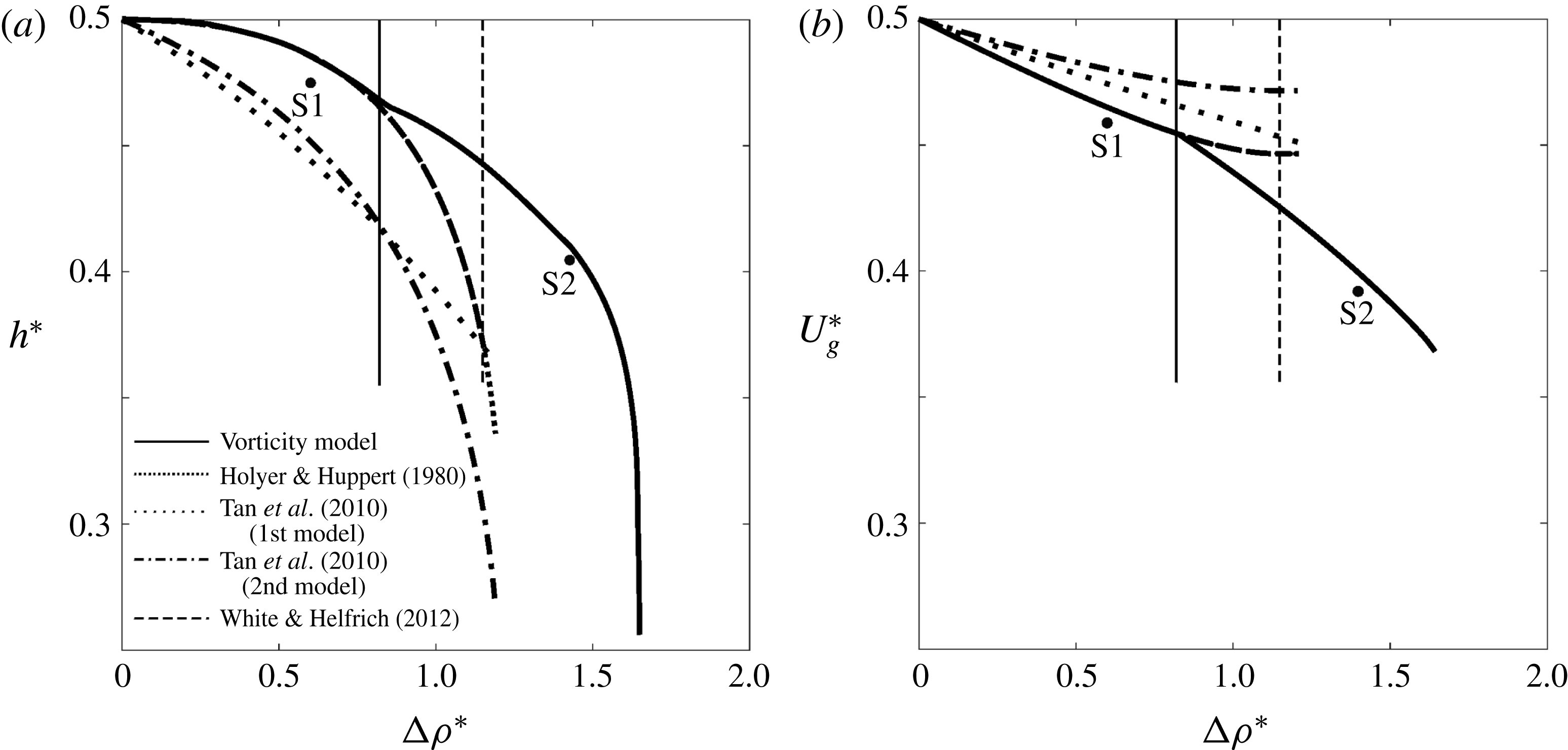
Similar to Holyer & Huppert (Reference Holyer and Huppert1980), the modelling approach by Tan et al. (Reference Tan, Nobes, Fleck and Flynn2010) employs the continuity equation for each ambient layer, along with the conservation of horizontal momentum for the entire control volume, and Bernoulli’s equation upstream of the stagnation point. The authors allow for dissipative effects by enforcing energy-conserving flow in only one of the ambient layers. Consequently, they suggest two different models: in the first model, they invoke Bernoulli’s equation within the dense ambient fluid and along the gravity current interface (
 $O-2o$
in figure 1
a), whereas in the second one, they employ Bernoulli’s principle within the light ambient fluid and along the interface between the two ambient fluids (
 $2i-3o$
in figure 1
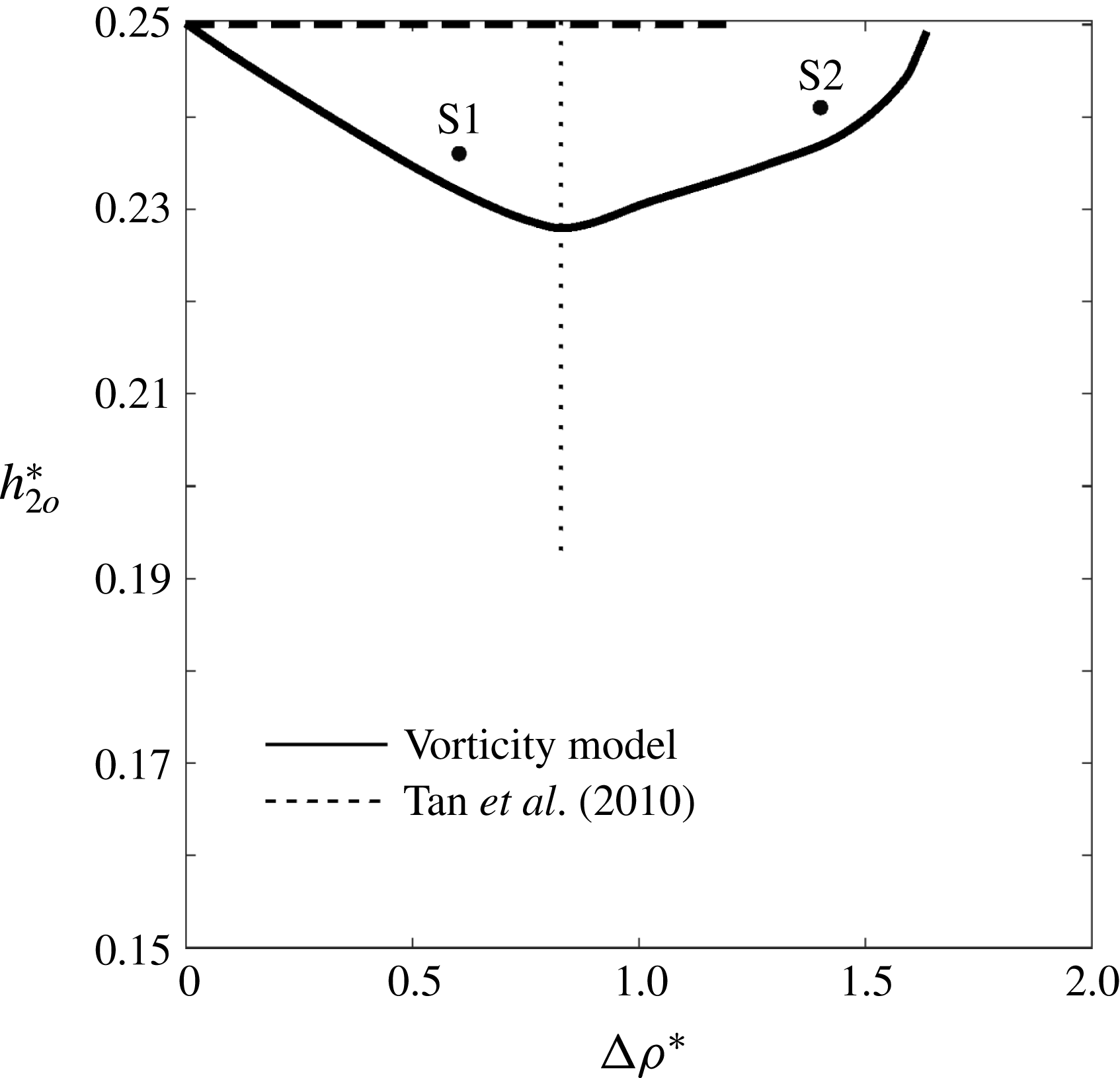
a). In order to close both models, Tan et al. (Reference Tan, Nobes, Fleck and Flynn2010) assume that the change
 $\unicode[STIX]{x1D702}$
in the ambient interface height from far upstream to far downstream is related to the channel height
 $H$
and the ambient interface height
 $h_{1i}$
at the inflow boundary as
 $$\begin{eqnarray}\unicode[STIX]{x1D702}={\textstyle \frac{1}{2}}(H-h_{1i}),\end{eqnarray}$$
which leads to
 $h_{2o}=h_{2i}/2$
. They base this empirical assumption on the examination of two limiting cases: (i)
 $h_{1i}\rightarrow 0$
, for which the energy-conserving solution of Benjamin (Reference Benjamin1968) predicts
 $h/H\rightarrow 0.5$
, so that
 $\unicode[STIX]{x1D702}/H\rightarrow 0.5$
; and (ii)
 $h_{1i}\rightarrow H$
, for which the upper layer vanishes, i.e.
 $\unicode[STIX]{x1D702}\rightarrow 0$
. Assuming that
 $\unicode[STIX]{x1D702}$
varies linearly between these two limits, they arrive at (1.1). The authors compare their model predictions to experimental and numerical results, and observe good agreement for various flow properties and moderate values of
 $\unicode[STIX]{x0394}\unicode[STIX]{x1D70C}$
. For large values of
 $\unicode[STIX]{x0394}\unicode[STIX]{x1D70C}$
the agreement deteriorates, as will be discussed further in § 6.
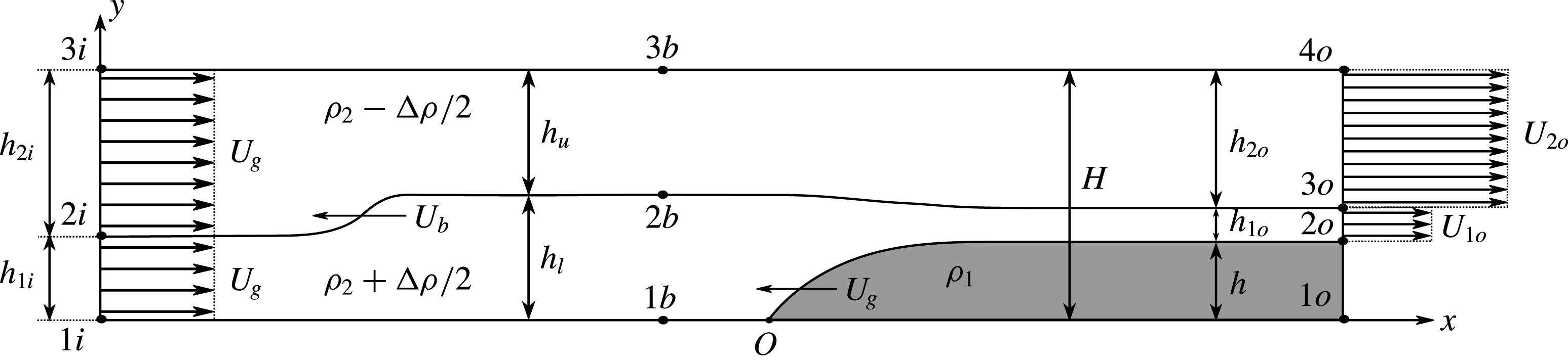
White & Helfrich (Reference White and Helfrich2012) further develop the analytical model of Holyer & Huppert (Reference Holyer and Huppert1980) for steady-state gravity currents, by allowing for equal head losses in both ambient layers. They also propose a model that incorporates a left-propagating internal bore when the flow over the gravity current is critical. Towards this end, they consider the flow configuration shown in figure 2. We note that, in contrast to C2 or C3 in figure 1, White & Helfrich (Reference White and Helfrich2012) do not incorporate an expansion wave in their analytical model, although they investigate it in their numerical simulations. To obtain the properties of the upstream bore they employ the model of Klemp, Rotunno & Skamarock (Reference Klemp, Rotunno and Skamarock1997), which conserves energy in the lower (expanding) layer. White & Helfrich (Reference White and Helfrich2012) find that the largest, fastest propagating bore forms when
 $h_{l}=H/2$
, which is consistent with the observations of Klemp et al. (Reference Klemp, Rotunno and Skamarock1997) and Khodkar, Nasr-Azadani & Meiburg (Reference Khodkar, Nasr-Azadani and Meiburg2017). An energy analysis of this bore in isolation shows the flow to be energy conserving under these conditions. Furthermore, in order to close their system of equations, they set the head loss along the gravity current interface to zero, arguing that the dissipation in the gravity current region is insignificant compared to that in the bore region.
Schematic of the model by White & Helfrich (Reference White and Helfrich2012), adapted from their paper. An upstream bore is assumed to exist, with
 $h_{l}=H/2$
.

The situation of two-layer stratified flows over topography is closely related to gravity currents propagating into a two-layer stratified ambients, although subtle differences exist, as discussed by Flynn, Ungarish & Tan (Reference Flynn, Ungarish and Tan2012). First and foremost, for flow over a solid topography, the height and shape of the obstacle can be prescribed independently of the flow velocity. On the other hand, the height and propagation velocity of a gravity current depend on each other. This is a consequence of the deformability of the gravity current, which renders its shape a function of the ambient flow conditions. These distinctions need to be kept in mind when referencing the terminology of Rottman & Simpson (Reference Rottman and Simpson1989). Pioneering experiments for two-layer flows over topography are described in Baines (Reference Baines1984), including the existence of sub- and supercritical flow regimes, as well as upstream-propagating expansion waves and internal bores. Baines (Reference Baines1984) furthermore discusses an analytical model based on the shallow-water equations that captures the dynamics of a subcritical–supercritical flow with an upstream wave, and he assesses the energy dissipation of the flow. Related investigations were carried out by Baines & Davies (Reference Baines and Davies1980), who categorize all possible flow regimes by defining two dimensionless parameters in the form of
 $D_{o}=h/h_{1i}$
and the Froude number
 $F_{o}=U/\sqrt{h_{1i}g\unicode[STIX]{x0394}\unicode[STIX]{x1D70C}/\unicode[STIX]{x1D70C}_{2}}$
, where
 $U$
and
 $h_{1i}$
indicate the obstacle velocity and the upstream ambient interface height, respectively, and
 $g$
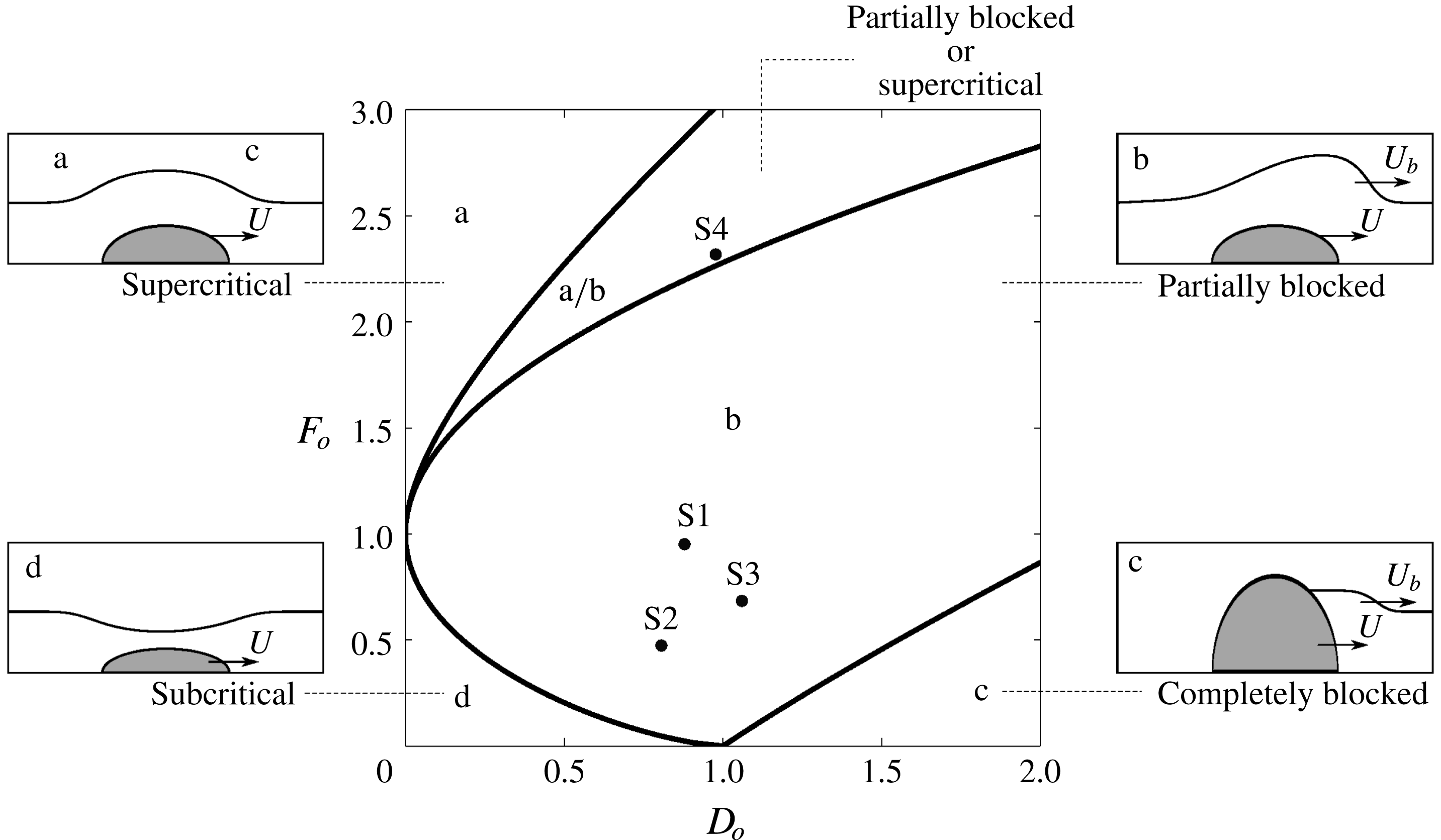
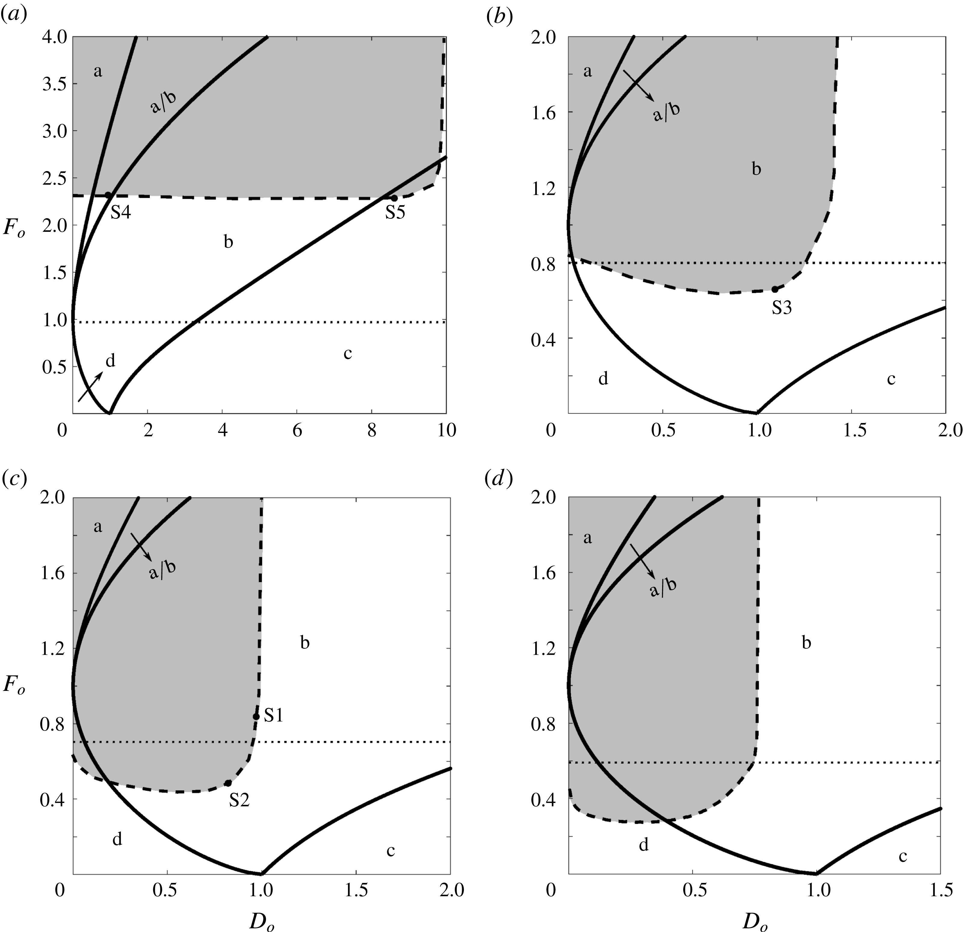
is the gravitational acceleration. Note that the obstacle velocity is related to the gravity current velocity in our study. Both Baines & Davies (Reference Baines and Davies1980) and Rottman & Simpson (Reference Rottman and Simpson1989) identify four different flow regimes, viz. supercritical, subcritical, partially blocked and completely blocked flows, shown as a, b, c and d in figure 3, respectively. Supercritical flows, in which an upstream-propagating wave does not appear, correspond to configuration C1 in figure 1(a). They can arise only for
 $F_{o}>1$
. Partially and completely blocked flows give rise to waves that propagate upstream with velocity
 $U_{b}$
, as shown in figure 3. The dynamics of partially blocked flows is analogous to that of C2- and C3-type flows, shown in figures 1(b) and 1(c), respectively. Figure 3 illustrates the regions corresponding to each of these regimes for two-layer stratified flows over solid obstacles, along with a schematic of their behaviour. Rottman & Simpson (Reference Rottman and Simpson1989) also compare their experimental results to the analytical model of Crook (Reference Crook, Lilly and Gal-Chen1983), as well as to the numerical investigations of Crook (Reference Crook1984) and Crook & Miller (Reference Crook and Miller1985), and they observe good qualitative and quantitative agreement.
Flow regimes for two-layer stratified flows over a streamlined obstacle, with the upper layer being infinitely deep, adapted from Rottman & Simpson (Reference Rottman and Simpson1989). S1 to S4 denote direct numerical simulations to be discussed in the next section.

White & Helfrich (Reference White and Helfrich2012) employ a slightly different classification scheme for gravity currents entering two-layer stratified ambients, by defining the two dimensionless parameters
 $F_{o}=U_{g}/c_{o}$
, and
 $D_{o}=h/h_{1i}$
. Here
 $c_{o}=\sqrt{g\unicode[STIX]{x0394}\unicode[STIX]{x1D70C}/\unicode[STIX]{x1D70C}_{2}h_{1i}(1-h_{1i}/H)}$
represents the linear long wave speed, so that the resulting Froude number is different from that defined by Rottman & Simpson (Reference Rottman and Simpson1989). This difference becomes insignificant for small values of
 $h_{1i}/H$
, which is the regime of interest to Rottman & Simpson (Reference Rottman and Simpson1989). White & Helfrich (Reference White and Helfrich2012) identify five different flow regimes, including subcritical gravity currents with a depression wave propagating along the ambient interface, gravity currents leading to the formation of an internal bore travelling along the ambient interface that is followed by an expansion wave (their flow regime III), as well as supercritical gravity currents without upstream-propagating disturbances. Their flow regime III corresponds to the partially blocked flows of Rottman & Simpson (Reference Rottman and Simpson1989), and to configuration C3 sketched in figure 1(c). Similarly, their sub- and supercritical flow regimes correspond to those of Rottman & Simpson (Reference Rottman and Simpson1989). White & Helfrich (Reference White and Helfrich2012) compare their model predictions to simulation results based on the Euler equations in the Boussinesq limit. They observe good agreement for sub- and supercritical gravity currents, while for flows with an upstream internal bore and/or expansion wave the discrepancy becomes more substantial.
In the following, we extend the vorticity-based modelling approach originally introduced by Borden & Meiburg (Reference Borden and Meiburg2013a ,Reference Borden and Meiburg b ) for gravity currents and internal bores, to the flow configurations shown in figure 1. This approach incorporates the momentum conservation principle in its vorticity form along the individual interfaces, thereby reducing the need for empirical closure assumptions based on energy considerations. The resulting models enable us to predict the propagation velocities of the gravity current and any upstream-propagating disturbances, as well as the ambient layer velocities and depths at the outflow boundary. Section 2 discusses direct numerical simulations (DNS) for the different flow regimes. In § 3, we present the development of vorticity-based models for these regimes, and we discuss their energetics. Section 4 provides predictions based on the vorticity models, which are subsequently compared to the DNS simulation results in § 5, and to earlier models by other authors in § 6. Section 7 summarizes the findings of the current work and gives some concluding remarks.
2 DNS simulations
To demonstrate the distinct features that characterize the different flow regimes, and to obtain quantitative information that can subsequently be compared to model predictions, we now proceed to discuss representative two-dimensional DNS simulation results. The DNS data were obtained with our code TURBINS, which has been described and validated in detail by Nasr-Azadani & Meiburg (Reference Nasr-Azadani and Meiburg2011) and Nasr-Azadani, Hall & Meiburg (Reference Nasr-Azadani, Hall and Meiburg2013). TURBINS is a finite-difference solver based on a fractional step projection method, along with total variation diminishing third-order Runge–Kutta (TVD-RK3) time integration. It solves the unsteady, incompressible Navier–Stokes equations in the Boussinesq limit
 $$\begin{eqnarray}\displaystyle & \displaystyle \unicode[STIX]{x1D735}\boldsymbol{\cdot }\boldsymbol{u}^{\ast }=0, & \displaystyle\end{eqnarray}$$
 $$\begin{eqnarray}\displaystyle & \displaystyle \frac{\unicode[STIX]{x2202}\unicode[STIX]{x1D70C}^{\ast }}{\unicode[STIX]{x2202}t^{\ast }}+\boldsymbol{u}^{\ast }\boldsymbol{\cdot }\unicode[STIX]{x1D735}\unicode[STIX]{x1D70C}^{\ast }=\frac{1}{Pe}\unicode[STIX]{x1D6FB}^{2}\unicode[STIX]{x1D70C}^{\ast }, & \displaystyle\end{eqnarray}$$
 $$\begin{eqnarray}\displaystyle & \displaystyle \frac{\unicode[STIX]{x2202}\boldsymbol{u}^{\ast }}{\unicode[STIX]{x2202}t^{\ast }}+\boldsymbol{u}^{\ast }\boldsymbol{\cdot }\unicode[STIX]{x1D735}\boldsymbol{u}^{\ast }=-\unicode[STIX]{x1D735}p^{\ast }+\frac{1}{Re}\unicode[STIX]{x1D6FB}^{2}\boldsymbol{u}^{\ast }+\unicode[STIX]{x1D70C}^{\ast }\boldsymbol{e}^{g}. & \displaystyle\end{eqnarray}$$
The above system has been rendered dimensionless by introducing the characteristic scales
 $$\begin{eqnarray}\boldsymbol{x}^{\ast }=\frac{\boldsymbol{x}}{H},\quad \boldsymbol{u}^{\ast }=\frac{\boldsymbol{u}}{\sqrt{g^{\prime }H}},\end{eqnarray}$$
 $$\begin{eqnarray}t^{\ast }=\frac{t}{\sqrt{H/g^{\prime }}},\quad \unicode[STIX]{x1D70C}^{\ast }=\frac{\unicode[STIX]{x1D70C}-\unicode[STIX]{x1D70C}_{2}}{\unicode[STIX]{x1D70C}_{1}-\unicode[STIX]{x1D70C}_{2}},\end{eqnarray}$$
 $$\begin{eqnarray}\unicode[STIX]{x0394}\unicode[STIX]{x1D70C}^{\ast }=\frac{\unicode[STIX]{x0394}\unicode[STIX]{x1D70C}}{\unicode[STIX]{x1D70C}_{1}-\unicode[STIX]{x1D70C}_{2}},\quad p^{\ast }=\frac{p}{\unicode[STIX]{x1D70C}_{2}g^{\prime }H},\end{eqnarray}$$
with the
 $^{\ast }$
-symbol indicating dimensionless quantities and
 $\boldsymbol{e}^{g}$
representing the unit vector in the direction of gravity. As dimensionless parameters we obtain
 $Re=\sqrt{g^{\prime }H}H/\unicode[STIX]{x1D708}$
and
 $Pe=\sqrt{g^{\prime }H}H/D$
, where
 $g^{\prime }=g(\unicode[STIX]{x1D70C}_{1}-\unicode[STIX]{x1D70C}_{2})/\unicode[STIX]{x1D70C}_{2}$
;
 $\unicode[STIX]{x1D708}$
and
 $D$
denote the kinematic viscosity and the diffusivity of the density field, respectively. The simulations are conducted in a reference frame that is moving with velocity
 $U_{g}^{\ast }$
, which is close to the gravity current front velocity. We impose no-flux conditions for the density field along with free-slip conditions for the velocity field at the upper and lower walls. At the inflow boundary we specify Dirichlet conditions that prescribe the ambient layer heights, velocities and densities. The outflow boundary is handled by a convective condition of the form
 $$\begin{eqnarray}\frac{\unicode[STIX]{x2202}q^{\ast }}{\unicode[STIX]{x2202}t^{\ast }}+\bar{U}^{\ast }\frac{\unicode[STIX]{x2202}q^{\ast }}{\unicode[STIX]{x2202}x^{\ast }}=0,\end{eqnarray}$$
where
 $q^{\ast }$
can be any flow quantity, and
 $\bar{U}^{\ast }$
is taken as the maximum velocity in the domain. Initial conditions for the gravity current height and the ambient layer thicknesses above the gravity current, as well as the velocity
 $U_{g}^{\ast }$
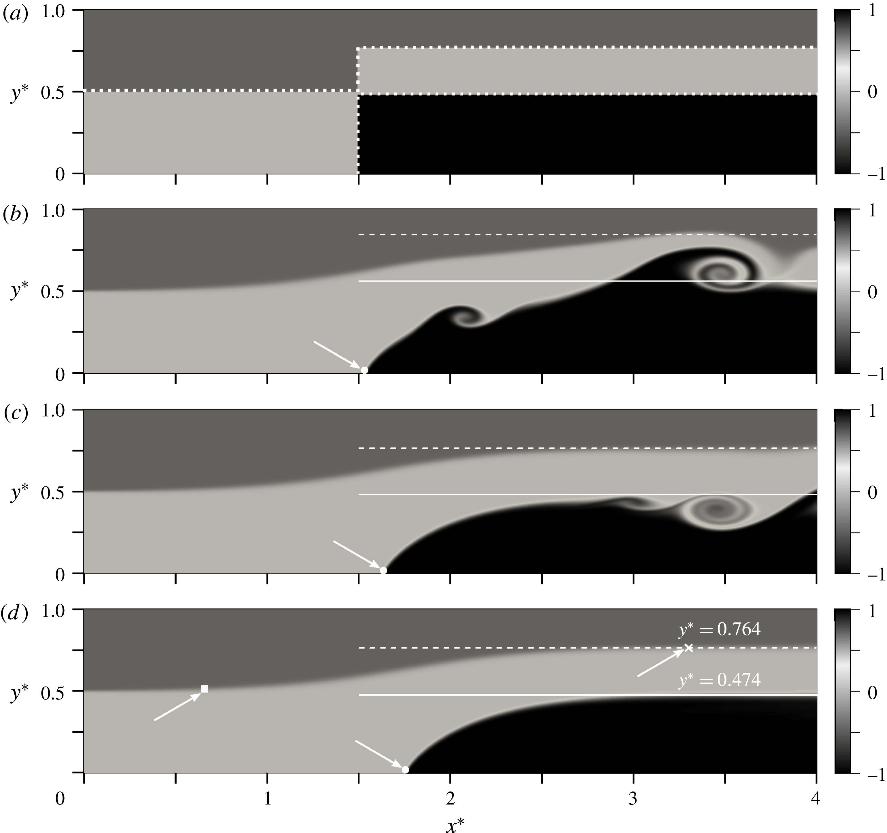
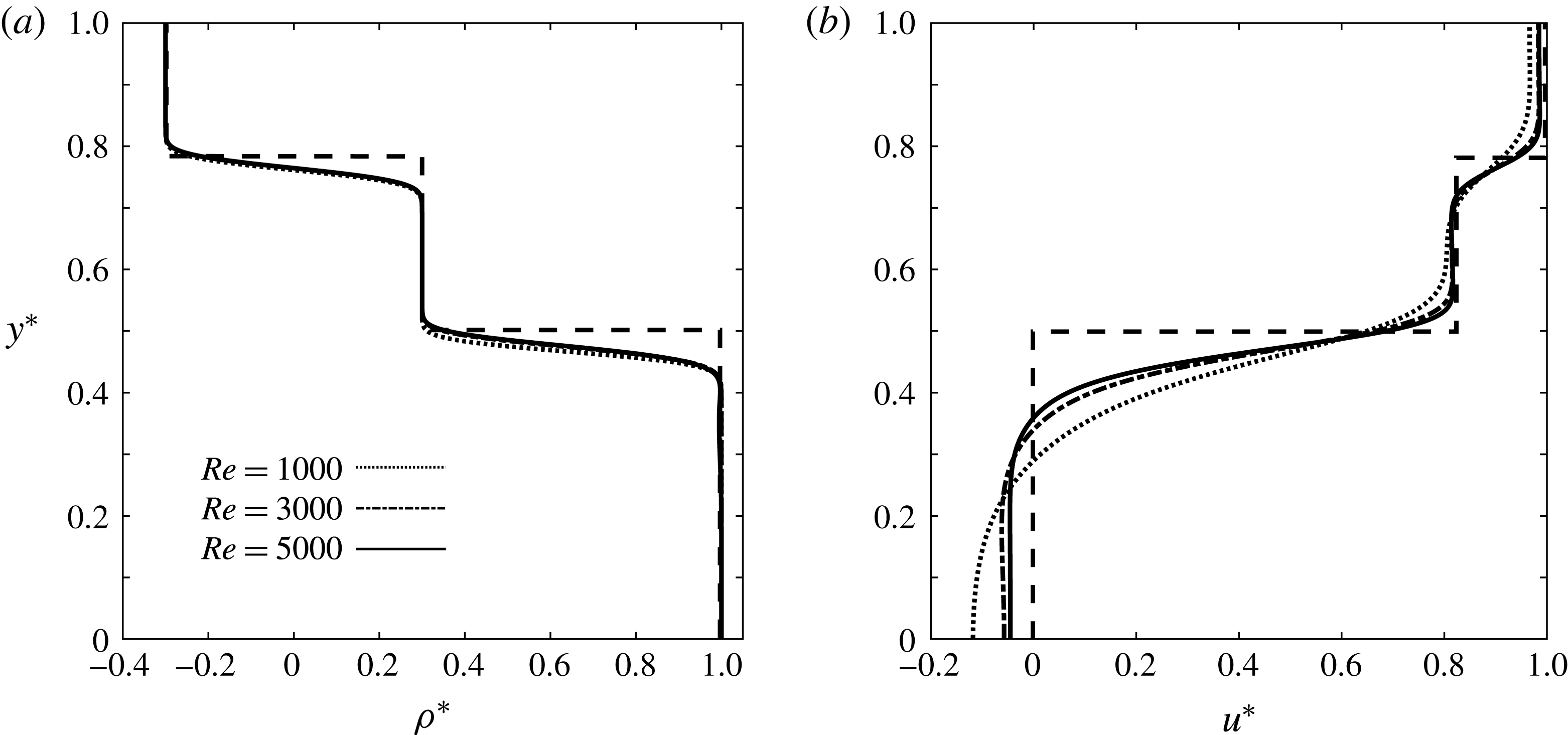
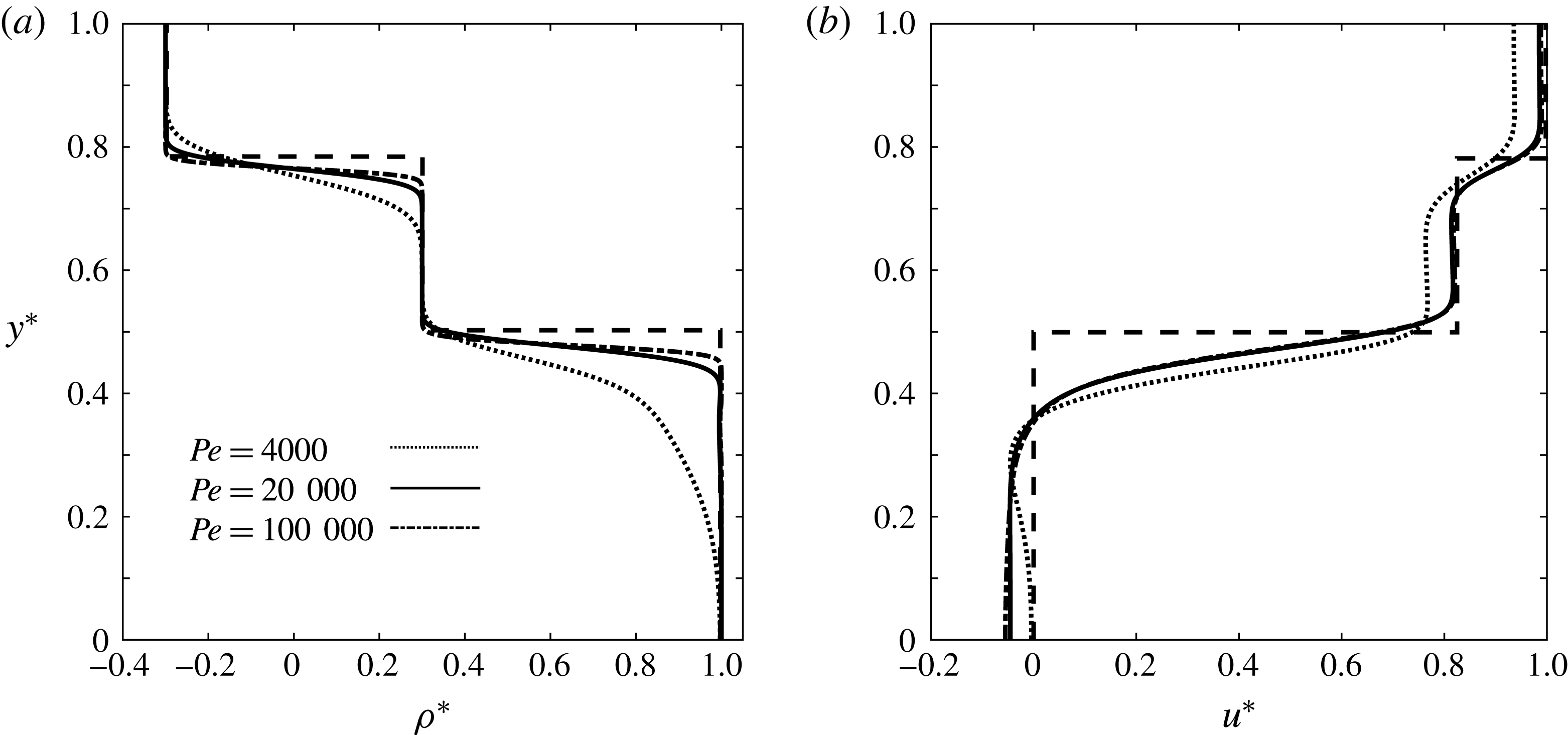
of the moving reference frame, are specified based on the simplified models to be derived in § 3, as exemplified by figure 4(a). We explored a range of initial conditions for the interfacial shapes, but found the emerging quasisteady flow features to be quite robust. The domain size
 $L_{x}\times L_{y}$
is selected according to whether or not an upstream-propagating expansion wave is expected to form. The uniform grid spacing of
 $\unicode[STIX]{x0394}x^{\ast }=0.004$
and
 $\unicode[STIX]{x0394}y^{\ast }=0.003$
is identical for all simulations, and the time step
 $\unicode[STIX]{x0394}t^{\ast }$
is taken according to the Courant–Friedrichs–Lewy (CFL) stability criterion. Table 1 summarizes the parameters of five simulations that will be discussed in some detail.
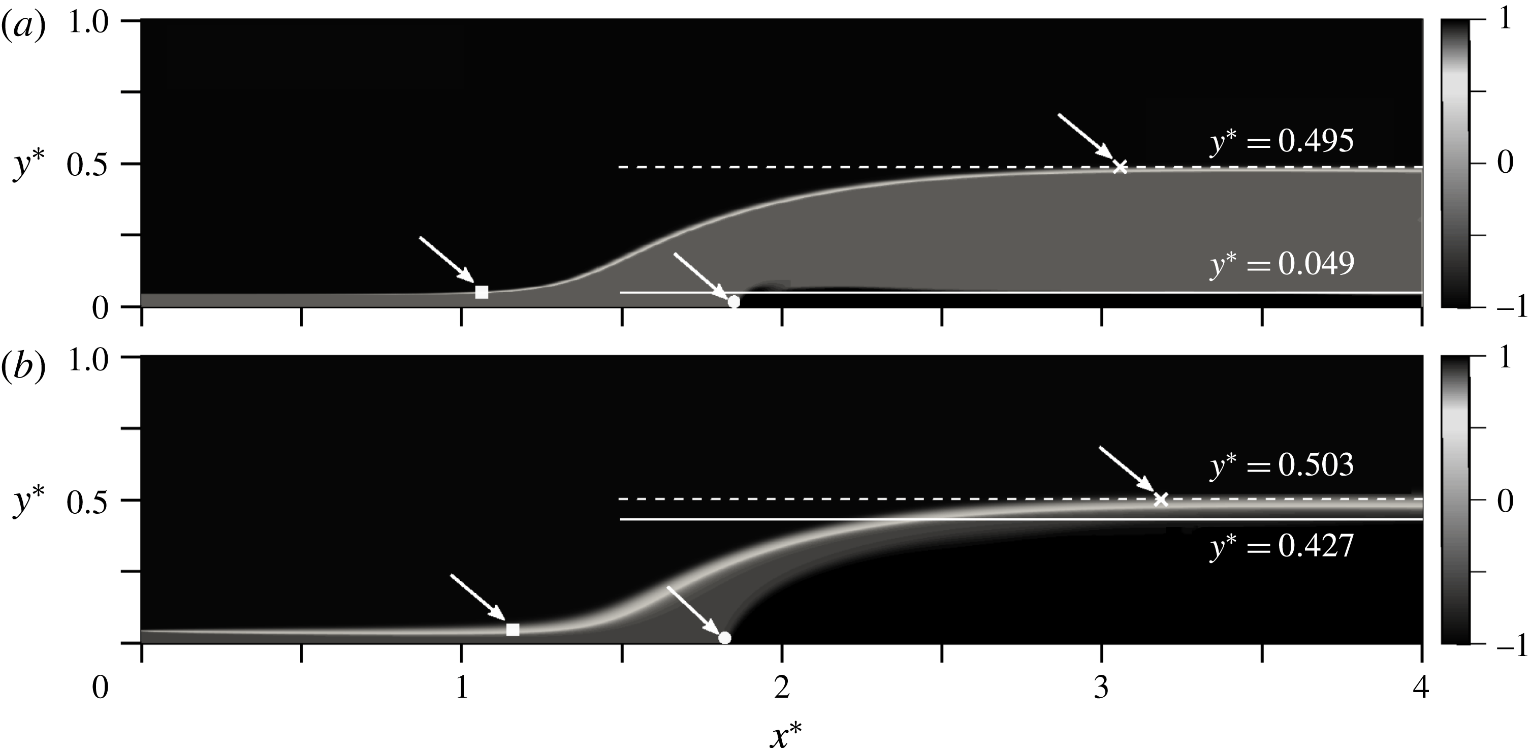
Temporal evolution of the density field for simulation S1, at
 $t^{\ast }=0$
(a), 3 (b), 10 (c) and 20 (d). The simulation parameters are
 $h_{1i}^{\ast }=0.5$
,
 $\unicode[STIX]{x0394}\unicode[STIX]{x1D70C}^{\ast }=0.6$
,
 $Re=5000$
and
 $Pe=20\,000$
. The initial conditions are prescribed according to the simplified model for configuration C1 derived in § 3. The simulation shows the evolution of a steady flow field without upstream-propagating disturbances. The transient Kelvin–Helmholtz vortices forming at the interface are swept outside the computational domain, reflecting their convectively unstable nature. The white horizontal solid and dashed lines represent the quasisteady gravity current height and the interface location between the ambient layers at the outflow, respectively. The white circle, square and cross indicate
 $x_{f}^{\ast }$
,
 $x_{l}^{\ast }$
and
 $x_{r}^{\ast }$
; cf. the discussion in the text.

Parameters of the DNS simulations to be discussed in this section.

2.1 Partially blocked flows
Figure 4 illustrates the temporal evolution of the density field for simulation S1. Transient, convectively unstable Kelvin–Helmholtz waves along the gravity current interface are soon washed out of the control volume, and a quasisteady state evolves. We remark that for some simulations involving larger values of
 $Re$
(not shown) the KH instabilities remained within the computational domain, so that a strictly quasisteady state did not emerge.
In order to compute the gravity current thickness, we mark the gravity current fluid initially by a passive dye of concentration
 $c_{d}^{\ast }=1$
. This dye has the same diffusivity as the density field. The local dimensionless height
 $d^{\ast }$
of the gravity current is then obtained as
 $$\begin{eqnarray}d^{\ast }(x^{\ast },t^{\ast })=\int _{0}^{1}c_{d}^{\ast }(x^{\ast },y^{\ast },t^{\ast })\,\text{d}y^{\ast }.\end{eqnarray}$$
The gravity current front location
 $x_{f}^{\ast }$
is defined as the leftmost point at which
 $d^{\ast }$
exceeds 0.01. The local thicknesses
 $d_{1}^{\ast }$
and
 $d_{2}^{\ast }$
of the ambient layers can be obtained analogously from corresponding passive dye fields. We furthermore identify the right and left edges of the ambient interfacial wave,
 $x_{r}^{\ast }$
and
 $x_{l}^{\ast }$
, in the following fashion: to obtain
 $x_{r}^{\ast }$
as a function of time, we sweep the ambient interface from the current tip towards the outflow boundary and evaluate
 $x_{r}^{\ast }$
as the first point at which
 $|\unicode[STIX]{x2202}(d^{\ast }+d_{1}^{\ast })/\unicode[STIX]{x2202}x^{\ast }|<0.01$
.
 $x_{l}^{\ast }$
is taken as the location of the leftmost point of the ambient interface where
 $d_{1}^{\ast }-h_{1i}^{\ast }>0.01$
. For those cases in which the flow gives rise to an internal bore propagating ahead of the expansion fan, this procedure yields the front location
 $x_{b}^{\ast }$
of the bore. In the presence of a bore, the location
 $x_{l}^{\ast }$
of the left edge of the expansion wave is then defined as the first point to the right of the bore at which
 $\unicode[STIX]{x2202}d_{1}^{\ast }/\unicode[STIX]{x2202}x^{\ast }|_{x^{\ast }}-\unicode[STIX]{x2202}d_{1}^{\ast }/\unicode[STIX]{x2202}x^{\ast }|_{x^{\ast }-\unicode[STIX]{x0394}x^{\ast }}<0$
. This definition is based on the rapid fall of the ambient interface slope as it transitions from the bore to the expansion fan region. In some cases this decrease occurs only very close to the gravity current tip, so that the disturbance takes the form of an expansion fan without a leading bore.
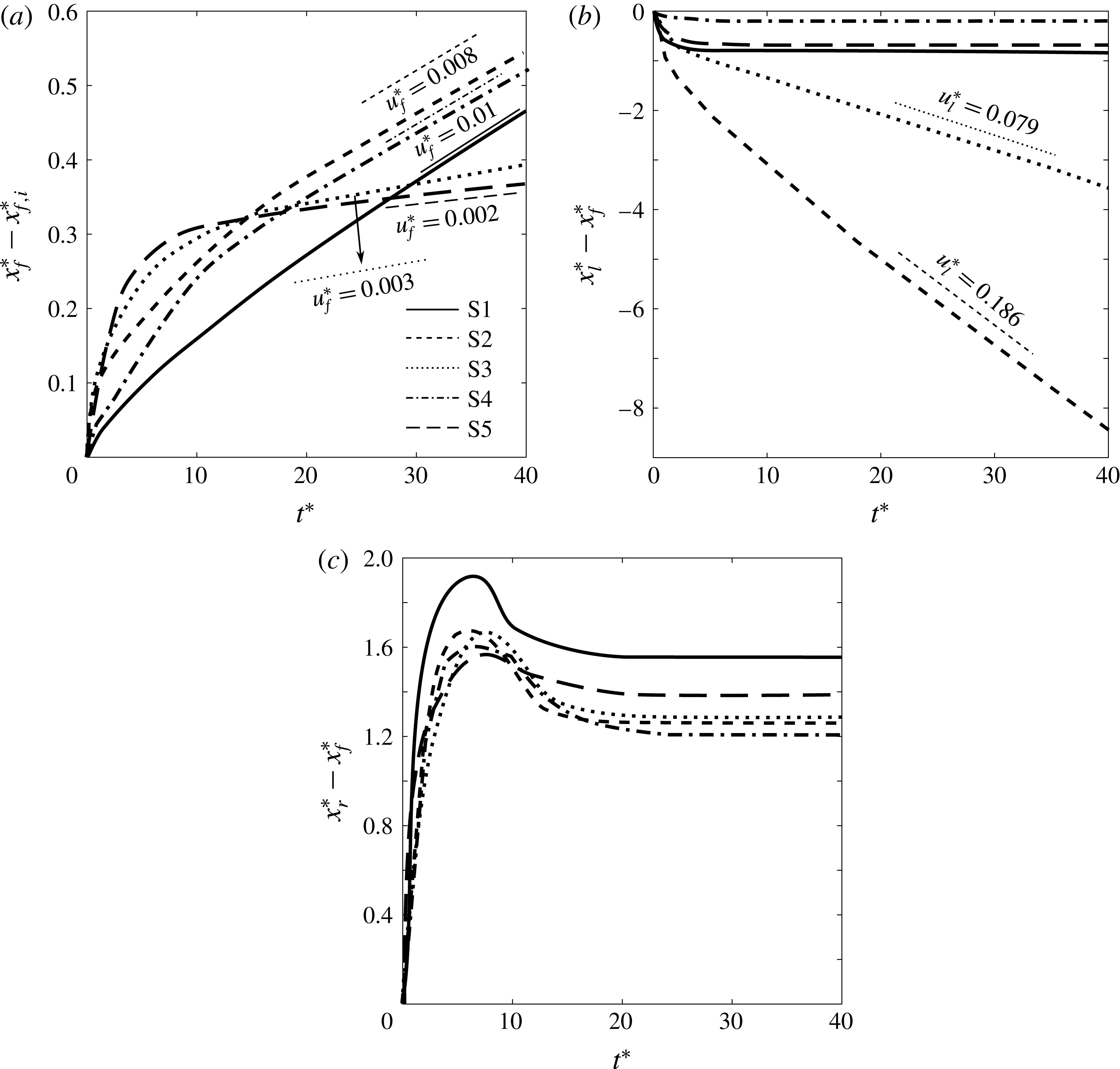
Within the moving reference frame of the simulation, figure 5(a) depicts the displacement with time of the gravity current tip
 $x_{f}^{\ast }$
, relative to its initial location
 $x_{f,i}^{\ast }$
, for all simulations of table 1. In all cases the front velocity
 $\text{d}x_{f}^{\ast }/\text{d}t^{\ast }$
initially varies with time, but eventually settles down to a constant value
 $u_{f}^{\ast }$
. The front velocity in the laboratory frame is then obtained as
 $$\begin{eqnarray}U_{g,lab}^{\ast }=U_{g}^{\ast }-u_{f}^{\ast }.\end{eqnarray}$$
DNS results for the temporal evolution of (a) the displacement of the gravity current tip
 $x_{f}^{\ast }$
with respect to its initial location
 $x_{f,i}^{\ast }$
, (b) the displacement of the expansion wave’s left edge
 $x_{l}^{\ast }$
relative to the gravity current front location
 $x_{f}^{\ast }$
and (c) the distance of the right edge
 $x_{r}^{\ast }$
of the expansion fan from the current tip, evaluated for the simulations of table 1. The straight line segments indicate the quasisteady velocities of the corresponding features in the moving reference frame, which have been obtained by linear fits of the DNS results between
 $t^{\ast }=20$
and
 $t^{\ast }=40$
, when the flow properties have become nearly independent of time. Note that the quasisteady velocities vanish for simulations S1, S4 and S5 in panel (b), and for all simulations in panel (c).

Figure 5(b) displays the displacement of the left edge of the expansion wave
 $x_{l}^{\ast }$
with respect to the gravity current front location
 $x_{f}^{\ast }$
as a function of time, for all simulations. After a brief transitional phase,
 $x_{l}^{\ast }-x_{f}^{\ast }$
remains nearly constant with time for S1, S4 and S5, indicating that the left edge of the wave moves at the same speed as the current tip. On the other hand, for cases S2 and S3 the left edge of the wave travels faster than the current tip, so that a quasisteady flow configuration is not achieved, as will be discussed in the context of figures 6 and 7. Here the relative velocity of the left edge of the wave with respect to the front approaches a constant value
 $u_{l}^{\ast }$
for long times. In the laboratory frame, the left edge of the wave thus travels with velocity
 $$\begin{eqnarray}U_{l,lab}^{\ast }=U_{g,lab}^{\ast }+u_{l}^{\ast }.\end{eqnarray}$$
If the flow gives rise to a bore, as will be discussed in the following, the bore speed
 $u_{b}^{\ast }$
in the moving reference frame can be determined analogously, by tracking the temporal evolution of
 $x_{b}^{\ast }-x_{f}^{\ast }$
. The bore velocity in the laboratory frame is then obtained as
 $$\begin{eqnarray}U_{b,lab}^{\ast }=U_{g,lab}^{\ast }+u_{b}^{\ast }.\end{eqnarray}$$
The interface height
 $h_{l}^{\ast }$
at the left edge of the wave is evaluated as
 $$\begin{eqnarray}h_{l}^{\ast }=d_{1}^{\ast }(x_{l}^{\ast },t_{s}^{\ast }),\end{eqnarray}$$
where we take
 $t_{s}^{\ast }=35$
, which falls into the quasisteady range.
The distance of the expansion wave’s right edge from the gravity current tip
 $x_{r}^{\ast }-x_{f}^{\ast }$
is shown in figure 5(c) for all simulations. In all cases, this distance acquires a quasisteady value for sufficiently large times, which indicates that the right edge of the wave is anchored to the gravity current front.
In order to avoid any potential contamination from the outflow boundary, we evaluate the downstream values of the layer thicknesses some distance upstream of this boundary as
 $$\begin{eqnarray}\displaystyle & \displaystyle h^{\ast }=d^{\ast }(0.9L_{x},t_{s}^{\ast }), & \displaystyle\end{eqnarray}$$
 $$\begin{eqnarray}\displaystyle & \displaystyle h_{1o}^{\ast }=d_{1}^{\ast }(0.9L_{x},t_{s}^{\ast }), & \displaystyle\end{eqnarray}$$
 $$\begin{eqnarray}\displaystyle & \displaystyle h_{2o}^{\ast }=d_{2}^{\ast }(0.9L_{x},t_{s}^{\ast }), & \displaystyle\end{eqnarray}$$
at
 $t_{s}^{\ast }=35$
. The downstream velocities of the ambient fluid layers are obtained as the average horizontal velocity across the corresponding layer
 $$\begin{eqnarray}\displaystyle & \displaystyle U_{1o}^{\ast }=\frac{\displaystyle \int _{h^{\ast }}^{h^{\ast }+h_{1o}^{\ast }}u^{\ast }(0.9L_{x},y^{\ast },t_{s}^{\ast })\,\text{d}y^{\ast }}{h_{1o}^{\ast }}, & \displaystyle\end{eqnarray}$$
 $$\begin{eqnarray}\displaystyle & \displaystyle U_{2o}^{\ast }=\frac{\displaystyle \int _{h^{\ast }+h_{1o}^{\ast }}^{1}u^{\ast }(0.9L_{x},y^{\ast },t_{s}^{\ast })\,\text{d}y^{\ast }}{h_{2o}^{\ast }}, & \displaystyle\end{eqnarray}$$
for
 $t_{s}^{\ast }=35$
. The DNS results from this section will be compared to predictions by the vorticity model in § 5.
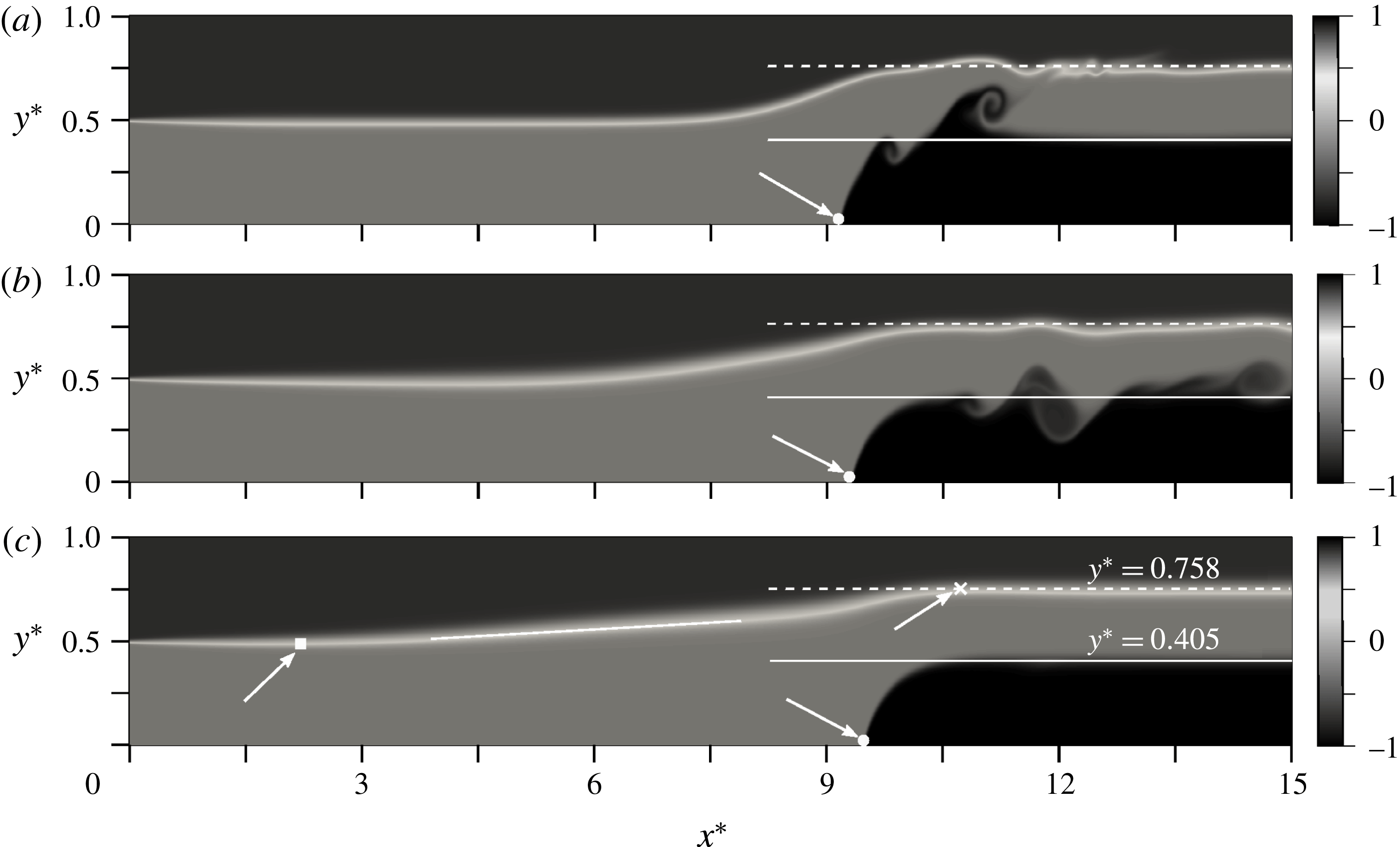
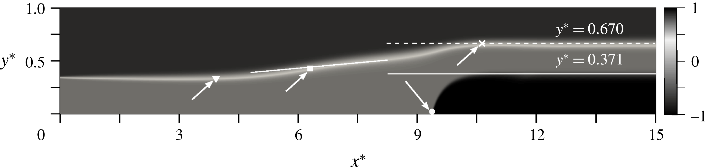
We now proceed to discuss simulations S2, which gives rise to an expansion fan, and S3, which results in the formation of an expansion fan and a bore. These observations are consistent with the findings of Tan et al. (Reference Tan, Nobes, Fleck and Flynn2010) and White & Helfrich (Reference White and Helfrich2012). As shown for simulation S2 in figure 6(c), in the absence of a bore the interfacial slope remains approximately constant over much of the wave region. If a bore is present, on the other hand, the slope of this interface undergoes a noticeable change at some intermediate location, as indicated by the white square in figure 7. For
 $h_{1i}^{\ast }$
close to one half, the bore becomes weak and increasingly difficult to observe. This is in line with the observations of Rottman & Simpson (Reference Rottman and Simpson1983), who noticed that the bore emerging ahead of the expansion wave in their partial lock-release experiments becomes difficult to identify when the ratio of the lock height to the tank depth is below 0.7. Similarly, the simulations of Khodkar et al. (Reference Khodkar, Nasr-Azadani and Meiburg2017) exhibit a more distinct bore when this ratio is 0.8 or greater.
Temporal evolution of the density field for simulation S2, at
 $t^{\ast }=5$
(a), 15 (b) and 35 (c). The simulation parameters are
 $h_{1i}^{\ast }=0.5$
,
 $\unicode[STIX]{x0394}\unicode[STIX]{x1D70C}^{\ast }=1.4$
,
 $Re=5000$
and
 $Pe=20\,000$
. The initial conditions are prescribed according to the simplified model for configuration C2 derived in § 3. The simulation gives rise to an upstream-propagating disturbance in the form of an expansion wave. The white horizontal solid and dashed lines represent the quasisteady gravity current height and the interface location between the ambient layers at the outflow, respectively. The white solid line tangent to the ambient interface shows that the interface height varies approximately linearly along the expansion wave. The white circle, square and cross indicate
 $x_{f}^{\ast }$
,
 $x_{l}^{\ast }$
and
 $x_{r}^{\ast }$
, respectively.

Snapshot of the density field for simulation S3 at
 $t^{\ast }=35$
. The simulation parameters are
 $h_{1i}^{\ast }=0.35$
,
 $\unicode[STIX]{x0394}\unicode[STIX]{x1D70C}^{\ast }=1.4$
,
 $Re=5000$
and
 $Pe=20\,000$
. The initial conditions are prescribed according to the simplified model for configuration C3 derived in § 3. The simulation gives rise to an upstream-propagating disturbance in the form of a bore, followed by an expansion wave. The white horizontal solid and dashed lines represent the quasisteady gravity current height and the interface location between the ambient layers at the outflow, respectively. The white solid line tangent to the ambient interface is intended to show that the bore region has a larger slope than the expansion fan region. The white circle, triangle, square and cross indicate
 $x_{f}^{\ast }$
,
 $x_{b}^{\ast }$
,
 $x_{l}^{\ast }$
and
 $x_{r}^{\ast }$
, respectively.

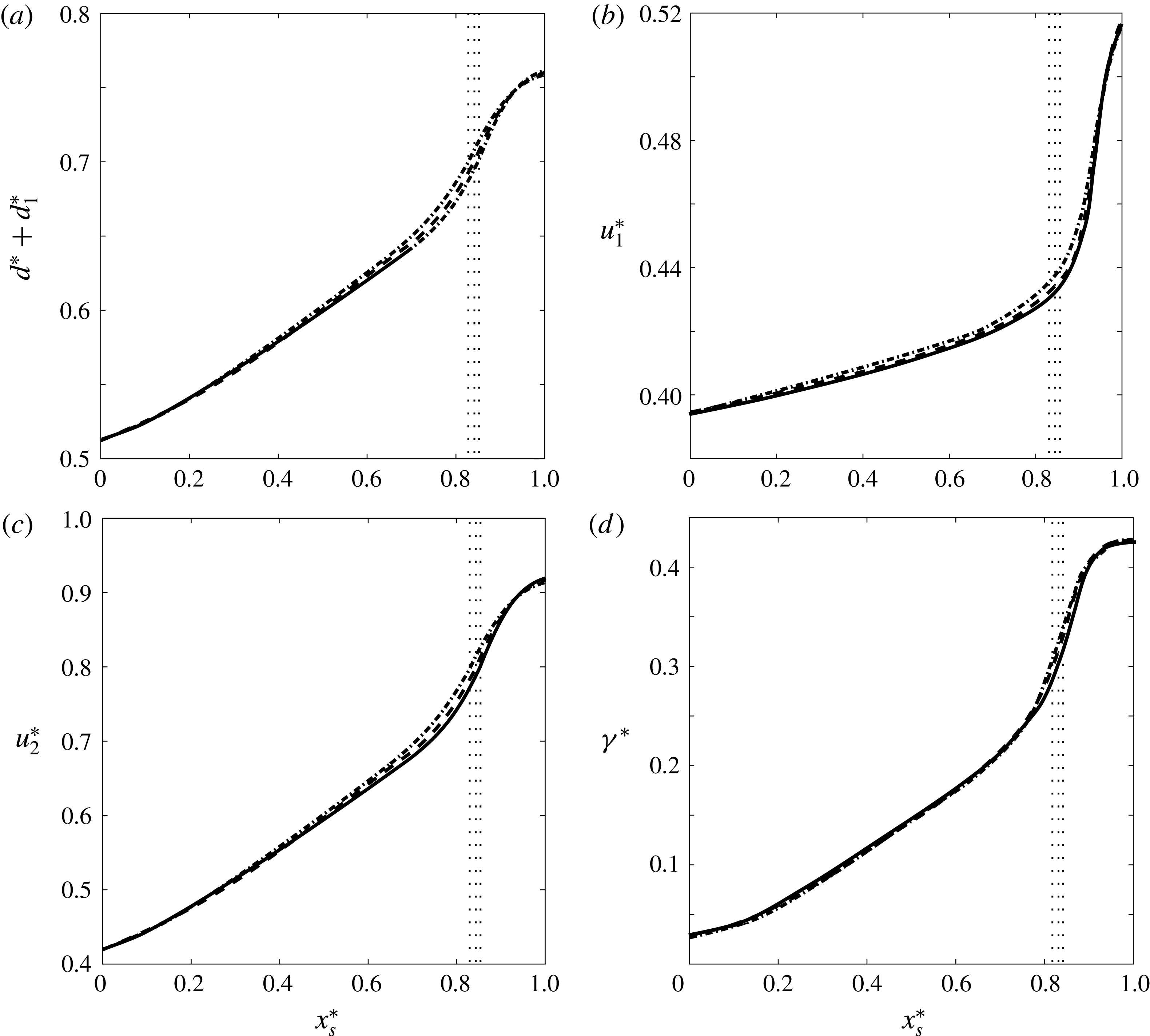
Simulation S2: DNS results for the spatial variation of various flow properties inside the wave region. (a) Interface height
 $d^{\ast }+d_{1}^{\ast }$
, (b) velocity
 $u_{1}^{\ast }$
of the lower ambient layer, (c) velocity
 $u_{2}^{\ast }$
of the upper ambient layer and (d) the interfacial vortex sheet strength
 $\unicode[STIX]{x1D6FE}^{\ast }=u_{2}^{\ast }-u_{1}^{\ast }$
. The results have been obtained for
 $t^{\ast }=25,30$
and 35, indicated by the dash-dotted, dashed and solid lines, respectively. The vertical dotted lines denote the location of the gravity current tip, with the leftmost line corresponding to
 $t^{\ast }=25$
and the rightmost one corresponding to
 $t^{\ast }=35$
. Over much of the expansion wave region, the respective flow properties are seen to vary approximately linearly.

We now analyse the variation of the ambient layer properties within the wave region, in preparation for developing simplified models in § 3. Panels (a–d) of figure 8 display the ambient interface height
 $d^{\ast }+d_{1}^{\ast }$
, the horizontal flow velocities within the lower and upper ambient layers
 $u_{1}^{\ast }$
and
 $u_{2}^{\ast }$
, and the vortex sheet strength
 $\unicode[STIX]{x1D6FE}^{\ast }=u_{2}^{\ast }-u_{1}^{\ast }$
, within the expansion wave region as functions of the scaled horizontal location
 $x_{s}^{\ast }=(x^{\ast }-x_{l}^{\ast })/(x_{r}^{\ast }-x_{l}^{\ast })$
, for simulation S2. Here,
 $u_{1}^{\ast }$
and
 $u_{2}^{\ast }$
are defined as
 $$\begin{eqnarray}\displaystyle & \displaystyle u_{1}^{\ast }(x^{\ast },t^{\ast })=\frac{\displaystyle \int _{d^{\ast }}^{d^{\ast }+d_{1}^{\ast }}u^{\ast }(x^{\ast },y^{\ast },t^{\ast })\,\text{d}y^{\ast }}{d_{1}^{\ast }}, & \displaystyle\end{eqnarray}$$
 $$\begin{eqnarray}\displaystyle & \displaystyle u_{2}^{\ast }(x^{\ast },t^{\ast })=\frac{\displaystyle \int _{d^{\ast }+d_{1}^{\ast }}^{1}u^{\ast }(x^{\ast },y^{\ast },t^{\ast })\,\text{d}y^{\ast }}{d_{2}^{\ast }}. & \displaystyle\end{eqnarray}$$
The results are shown for the three times
 $t^{\ast }=25$
, 30 and 35, when the Kelvin–Helmholtz instabilities have left the domain and the flow variables far up- and downstream have become time-independent. While the ambient interface height, as well as
 $u_{1}^{\ast }$
,
 $u_{2}^{\ast }$
and
 $\unicode[STIX]{x1D6FE}^{\ast }$
, vary approximately linearly along much of the wave region, they experience more abrupt changes in the vicinity of the gravity current front (vertical dotted lines in figure 8), due to the strong upward acceleration of the ambient fluid caused by the current nose.
We note that in terms of their dimensionless parameters, all three of the above simulations fall into the partially blocked regime identified by Rottman & Simpson (Reference Rottman and Simpson1989) for two-layer stratified flows over solid obstacles: cf. figure 3. However, as mentioned earlier, it is important to keep in mind the subtle differences between gravity current flows and those over solid obstacles; cf. the discussion in Flynn et al. (Reference Flynn, Ungarish and Tan2012). Consequently, the classification introduced by Rottman & Simpson (Reference Rottman and Simpson1989) does not transfer directly to the gravity current problem, which explains why only S2 and S3, but not S1, give rise to upstream-propagating waves.
2.2 Supercritical flow
In addition to the partially blocked flows with
 $U_{g,lab}^{\ast }>U_{l,lab}^{\ast }$
(or
 $u_{l}^{\ast }=0$
), there is another flow regime that does not give rise to upstream waves and can be modelled by C1. This supercritical region was introduced by Baines & Davies (Reference Baines and Davies1980) and is sketched in figure 3. Figure 9(a), which corresponds to S4 in table 1, reflects this flow regime.
Snapshots of the quasisteady density fields for simulations S4 (a) and S5 (b), at
 $t^{\ast }=20$
. The simulation parameters are
 $h_{1i}^{\ast }=0.05$
and
 $\unicode[STIX]{x0394}\unicode[STIX]{x1D70C}^{\ast }=1.89$
, and slightly different values of
 $Re$
and
 $Pe$
: cf. table 1. S4 and S5, while both corresponding to configuration C1, are classified as supercritical and partially blocked flows, respectively, by Rottman & Simpson (Reference Rottman and Simpson1989). The white horizontal solid and dashed lines represent the quasisteady gravity current height and the ambient interface location at the outflow. The white circles, squares and crosses indicate
 $x_{f}^{\ast }$
,
 $x_{l}^{\ast }$
and
 $x_{r}^{\ast }$
, respectively.

Consistent with figure 3, in order to achieve supercritical behaviour we take the ratio
 $D_{o}=h^{\ast }/h_{1i}^{\ast }\approx 1$
, while the Froude number
 $F_{o}=U_{g}^{\ast }/\sqrt{h_{1i}^{\ast }\unicode[STIX]{x0394}\unicode[STIX]{x1D70C}^{\ast }}$
needs to be sufficiently large. To increase
 $F_{o}$
we select a small value for
 $h_{1i}^{\ast }$
and focus on cases that yield large gravity current front velocities. According to the analytical model to be discussed in § 3, and corresponding results of § 4, for very small values of
 $h_{1i}^{\ast }$
,
 $U_{g}^{\ast }$
becomes largest when
 $\unicode[STIX]{x0394}\unicode[STIX]{x1D70C}^{\ast }\approx 2$
. Additionally, because
 $D_{o}\approx 1$
, the gravity current height needs to be small as well. For these reasons, in case S4 we choose
 $h_{1i}^{\ast }=h^{\ast }=0.05$
. Simulating flows of very thin gravity currents whose density is close to that of the lower ambient fluid layer, requires large values of
 $Re$
and
 $Pe$
.
For moderate values of
 $h_{1i}^{\ast }\gtrsim 0.15$
the simulations typically yielded only a single possible gravity current thickness for each
 $\unicode[STIX]{x0394}\unicode[STIX]{x1D70C}^{\ast }$
. On the other hand, for very small values of
 $h_{1i}^{\ast }$
we observed that gravity currents with two different heights might form for the same ambient density difference. Simulations S4 and S5, shown in figures 9(a) and 9(b), represent an example in this regard. These simulations have the same values for
 $h_{1i}^{\ast }$
and
 $\unicode[STIX]{x0394}\unicode[STIX]{x1D70C}^{\ast }$
, and slightly different values of
 $Re$
and
 $Pe$
, resulting in very different gravity current heights. According to Rottman & Simpson (Reference Rottman and Simpson1989), S5 would fall into the completely blocked flow regime for a two-layer flow over a solid obstacle. On the other hand, in our DNS simulations for gravity currents propagating into two-layer stratified ambients we never observed a completely blocked flow, i.e. a flow for which the ambient interface does not pass over the gravity current, even for very small lower ambient inflow thicknesses. Again, this reflects the differences between the solid obstacle and gravity current flows alluded to earlier. We note that, to the best of our knowledge, supercritical gravity currents with such small values for
 $h_{1i}^{\ast }$
and
 $h^{\ast }$
have not been observed experimentally or numerically in previous investigations.
3 Vorticity-based modelling
In the following we apply the vorticity-based modelling approach (Borden & Meiburg Reference Borden and Meiburg2013a ; Khodkar et al. Reference Khodkar, Nasr-Azadani and Meiburg2017) to gravity currents propagating into two-layer stratified ambients, for each of the configurations shown in figure 1.
3.1 Flows without upstream-propagating disturbance
The most basic flow configuration C1, as sketched in figure 1(a), is characterized by a smooth, steady ambient interface without upstream wave propagation. For a given gravity current height
 $h^{\ast }$
, and prescribed ambient densities and upstream layer thicknesses, we have five unknowns: the velocity
 $U_{g}^{\ast }$
of the gravity current, as well as the ambient velocities (
 $U_{1o}^{\ast }$
,
 $U_{2o}^{\ast }$
) and layer thicknesses (
 $h_{1o}^{\ast }$
,
 $h_{2o}^{\ast }$
) at the outflow boundary. In the reference frame moving with the gravity current front, the dimensionless mass conservation equations for the ambient layers read
 $$\begin{eqnarray}\displaystyle & \displaystyle U_{g}^{\ast }h_{1i}^{\ast }=U_{1o}^{\ast }h_{1o}^{\ast }, & \displaystyle\end{eqnarray}$$
 $$\begin{eqnarray}\displaystyle & \displaystyle U_{g}^{\ast }h_{2i}^{\ast }=U_{2o}^{\ast }h_{2o}^{\ast }. & \displaystyle\end{eqnarray}$$
Vorticity conservation along the top of the gravity current
 $O-2o$
and the interface between the ambient fluid layers
 $2i-3o$
results in
 $$\begin{eqnarray}\displaystyle & \displaystyle \frac{1}{2}{U_{1o}^{\ast }}^{2}=\frac{g_{1}^{\prime }}{g^{\prime }}h^{\ast }, & \displaystyle\end{eqnarray}$$
 $$\begin{eqnarray}\displaystyle & \displaystyle \frac{U_{1o}^{\ast }+U_{2o}^{\ast }}{2}(U_{2o}^{\ast }-U_{1o}^{\ast })=\frac{g_{2}^{\prime }}{g^{\prime }}(h_{1o}^{\ast }+h^{\ast }-h_{1i}^{\ast }), & \displaystyle\end{eqnarray}$$
where
 $$\begin{eqnarray}\displaystyle & \displaystyle \frac{g_{1}^{\prime }}{g^{\prime }}=\frac{\displaystyle \unicode[STIX]{x1D70C}_{1}-\left(\unicode[STIX]{x1D70C}_{2}+\frac{\unicode[STIX]{x0394}\unicode[STIX]{x1D70C}}{2}\right)}{\unicode[STIX]{x1D70C}_{1}-\unicode[STIX]{x1D70C}_{2}}, & \displaystyle\end{eqnarray}$$
 $$\begin{eqnarray}\displaystyle & \displaystyle \frac{g_{2}^{\prime }}{g^{\prime }}=\frac{\displaystyle \left(\unicode[STIX]{x1D70C}_{2}+\frac{\unicode[STIX]{x0394}\unicode[STIX]{x1D70C}}{2}\right)-\left(\unicode[STIX]{x1D70C}_{2}-\frac{\unicode[STIX]{x0394}\unicode[STIX]{x1D70C}}{2}\right)}{\unicode[STIX]{x1D70C}_{1}-\unicode[STIX]{x1D70C}_{2}}=\frac{\unicode[STIX]{x0394}\unicode[STIX]{x1D70C}}{\unicode[STIX]{x1D70C}_{1}-\unicode[STIX]{x1D70C}_{2}}. & \displaystyle\end{eqnarray}$$
A fifth equation is obtained from the geometrical constraint at the outflow boundary
 $$\begin{eqnarray}h^{\ast }+h_{1o}^{\ast }+h_{2o}^{\ast }=1.\end{eqnarray}$$
The above equations (3.1)–(3.4) and (3.7) represent a closed algebraic system for the five unknowns
 $U_{g}^{\ast }$
,
 $U_{1o}^{\ast }$
,
 $U_{2o}^{\ast }$
,
 $h_{1o}^{\ast }$
and
 $h_{2o}^{\ast }$
, so that empirical closure assumptions are not needed.
As an aside, we insert here a brief comment on the relationship between the head losses in the upper and lower layers, for the quasisteady flow of C1 in the moving reference frame. Within each layer, the head loss is of course constant along all streamlines, since the flow is irrotational. We write Bernoulli’s equation with a head loss in dimensionless form, for fluid elements immediately below and above the streamline
 $2i-3o$
:
 $$\begin{eqnarray}\displaystyle & \displaystyle p_{2i}^{\ast }+\frac{1}{2}{U_{g}^{\ast }}^{2}+\frac{\displaystyle \left(\unicode[STIX]{x1D70C}_{2}+\frac{\unicode[STIX]{x0394}\unicode[STIX]{x1D70C}}{2}\right)g}{\unicode[STIX]{x1D70C}_{2}g^{\prime }}h_{1i}^{\ast }=p_{3o}^{\ast }+\frac{1}{2}{U_{1o}^{\ast }}^{2}+\frac{\displaystyle \left(\unicode[STIX]{x1D70C}_{2}+\frac{\unicode[STIX]{x0394}\unicode[STIX]{x1D70C}}{2}\right)g}{\unicode[STIX]{x1D70C}_{2}g^{\prime }}(h^{\ast }+h_{1o}^{\ast })+\unicode[STIX]{x1D6E5}_{1}^{\ast },\qquad & \displaystyle\end{eqnarray}$$
 $$\begin{eqnarray}\displaystyle & \displaystyle p_{2i}^{\ast }+\frac{1}{2}{U_{g}^{\ast }}^{2}+\frac{\displaystyle \left(\unicode[STIX]{x1D70C}_{2}-\frac{\unicode[STIX]{x0394}\unicode[STIX]{x1D70C}}{2}\right)g}{\unicode[STIX]{x1D70C}_{2}g^{\prime }}h_{1i}^{\ast }=p_{3o}^{\ast }+\frac{1}{2}{U_{2o}^{\ast }}^{2}+\frac{\displaystyle \left(\unicode[STIX]{x1D70C}_{2}-\frac{\unicode[STIX]{x0394}\unicode[STIX]{x1D70C}}{2}\right)g}{\unicode[STIX]{x1D70C}_{2}g^{\prime }}(h^{\ast }+h_{1o}^{\ast })+\unicode[STIX]{x1D6E5}_{2}^{\ast }.\qquad & \displaystyle\end{eqnarray}$$
Here
 $\unicode[STIX]{x1D6E5}_{1}^{\ast }$
and
 $\unicode[STIX]{x1D6E5}_{2}^{\ast }$
represent the dimensionless head losses within the lower and upper ambient layers, respectively, scaled by
 $\unicode[STIX]{x1D6E5}_{ref}=\unicode[STIX]{x1D70C}_{2}g^{\prime }H$
. Subtracting (3.9) from (3.8) yields
 $$\begin{eqnarray}\displaystyle \unicode[STIX]{x1D6E5}_{1}^{\ast }-\unicode[STIX]{x1D6E5}_{2}^{\ast }=\frac{1}{2}({U_{2o}^{\ast }}^{2}-{U_{1o}^{\ast }}^{2})-\frac{g_{2}^{\prime }}{g^{\prime }}(h^{\ast }+h_{1o}^{\ast }-h_{1i}^{\ast }). & & \displaystyle\end{eqnarray}$$
The right-hand side of this equation vanishes according to (3.4), and we conclude that vorticity conservation immediately implies that both ambient layers have the same head loss. We will return to this point when discussing the assumptions underlying previous models of earlier investigators in § 6.
3.2 Propagation of a rarefaction wave towards the inflow boundary
Figure 1(b) displays configuration C2, a flow with a rarefaction wave travelling towards the inflow boundary, which causes the steady-state assumption to be invalid, even in the reference frame moving with the gravity current tip. The DNS results of § 2 show that the right edge
 $R$
of the wave remains stationary in the reference frame of the gravity current. The speed
 $U_{l}$
of the left edge
 $L$
of the wave is merely a function of the inflow conditions
 $$\begin{eqnarray}U_{l}^{\ast }=\sqrt{\unicode[STIX]{x0394}\unicode[STIX]{x1D70C}^{\ast }h_{1i}^{\ast }h_{2i}^{\ast }}\end{eqnarray}$$
(cf. Khodkar et al.
Reference Khodkar, Nasr-Azadani and Meiburg2017). We then need five additional equations to determine the remaining unknowns
 $U_{g}^{\ast }$
,
 $U_{1o}^{\ast }$
,
 $U_{2o}^{\ast }$
,
 $h_{1o}^{\ast }$
and
 $h_{2o}^{\ast }$
. These can again be obtained from the mass balances of the two ambient layers, the vorticity balances along the two interfaces and the geometrical constraint provided by (3.7), although the unsteadiness renders the equations slightly more complex. While the vorticity balance along the steady upper boundary of the gravity current is still given by (3.3), the unsteady evolution of the rarefaction wave modifies the other three equations.
In order to quantify the temporal changes of the ambient layer volumes, and of the circulation along the boundary separating these layers, we assume that the ambient interface height as well as the vortex sheet strength vary linearly within the wave region from
 $L$
to
 $R$
. The DNS results of § 2 above showed that this approximation holds to a good degree over much of the wave region, although it becomes questionable in the region immediately above the gravity current front: cf. figure 8(a). Hence it will be interesting to compare the predictions obtained on the basis of this approximation with the actual DNS results further below. Consequently, in the reference frame of the gravity current the mass balance for the deforming upper layer within control volume
 $L-3o-4o-L^{\prime }$
yields
 $$\begin{eqnarray}(U_{l}^{\ast }-U_{g}^{\ast })\frac{h_{2i}^{\ast }+h_{2o}^{\ast }}{2}=U_{l}^{\ast }h_{2i}^{\ast }-U_{2o}^{\ast }h_{2o}^{\ast }.\end{eqnarray}$$
Mass conservation for the entire channel
 $1i-1o-4o-3i$
results in
 $$\begin{eqnarray}\displaystyle U_{g}^{\ast }=U_{1o}^{\ast }h_{1o}^{\ast }+U_{2o}^{\ast }h_{2o}^{\ast }. & & \displaystyle\end{eqnarray}$$
To obtain an equation for the vorticity along the ambient interface
 $2i-3o$
, we start from the integral form of the inviscid vorticity conservation equation
 $$\begin{eqnarray}\displaystyle \frac{\text{d}}{\text{d}t^{\ast }}\int _{CV(t^{\ast })}\unicode[STIX]{x1D714}^{\ast }\,\text{d}A^{\ast }+\oint _{CS(t^{\ast })}\unicode[STIX]{x1D714}\boldsymbol{V}_{r}^{\ast }\boldsymbol{\cdot }\boldsymbol{n}\,\text{d}S^{\ast }=-\int _{CV(t^{\ast })}\frac{g_{2}^{\prime }}{g^{\prime }}\frac{\unicode[STIX]{x2202}\unicode[STIX]{x1D70C}^{\ast }}{\unicode[STIX]{x2202}x^{\ast }}\,\text{d}A^{\ast }, & & \displaystyle\end{eqnarray}$$
where
 $\unicode[STIX]{x1D714}^{\ast }=\unicode[STIX]{x1D714}/\sqrt{g^{\prime }/H}$
, and
 $CS$
denotes the boundary of the control volume that contains the ambient interface.
 $\boldsymbol{V}_{r}^{\ast }$
represents the relative flow velocity at this boundary. The temporal rate of change of the circulation inside the control volume is due to the elongation of the wave region resulting from the rarefaction wave propagation. The rate at which the wave region lengthens is given by
 $U_{l}^{\ast }-U_{g}^{\ast }$
. Based on the DNS results of § 2 (cf. figure 8
d), we assume that the vortex sheet strength varies linearly from
 $L$
to
 $R$
, so that its average value in the wave region is
 $(U_{2o}^{\ast }-U_{1o}^{\ast })/2$
. Hence we obtain
 $$\begin{eqnarray}\displaystyle \frac{\text{d}}{\text{d}t^{\ast }}\int _{CV(t^{\ast })}\unicode[STIX]{x1D714}^{\ast }\,\text{d}A^{\ast }=-\frac{1}{2}(U_{l}^{\ast }-U_{g}^{\ast })(U_{2o}^{\ast }-U_{1o}^{\ast }). & & \displaystyle\end{eqnarray}$$
There is no influx of vorticity into the control volume, and the shear at the outflow boundary yields
 $$\begin{eqnarray}\displaystyle \oint _{CS(t)}\unicode[STIX]{x1D714}^{\ast }\boldsymbol{V}_{r}^{\ast }\boldsymbol{\cdot }\boldsymbol{n}\,\text{d}S^{\ast }=-\frac{1}{2}(U_{2o}^{\ast }-U_{1o}^{\ast })(U_{2o}^{\ast }+U_{1o}^{\ast }). & & \displaystyle\end{eqnarray}$$
The baroclinic vorticity production term can be evaluated as
 $$\begin{eqnarray}\displaystyle -\!\int _{CV(t^{\ast })}\frac{g_{2}^{\prime }}{g^{\prime }}\frac{\unicode[STIX]{x2202}\unicode[STIX]{x1D70C}^{\ast }}{\unicode[STIX]{x2202}x^{\ast }}\,\text{d}A^{\ast }=-\unicode[STIX]{x0394}\unicode[STIX]{x1D70C}^{\ast }(h_{1o}^{\ast }+h^{\ast }-h_{1i}^{\ast }). & & \displaystyle\end{eqnarray}$$
By substituting (3.15)–(3.17) into (3.14), we obtain the vorticity equation in the form
 $$\begin{eqnarray}\displaystyle \frac{1}{2}(U_{l}^{\ast }-U_{g}^{\ast })(U_{2o}^{\ast }-U_{1o}^{\ast })+\frac{{U_{2o}^{\ast }}^{2}-{U_{1o}^{\ast }}^{2}}{2}=\unicode[STIX]{x0394}\unicode[STIX]{x1D70C}^{\ast }(h^{\ast }+h_{1o}^{\ast }-h_{1i}^{\ast }). & & \displaystyle\end{eqnarray}$$
The system of equations (3.3), (3.12), (3.13) and (3.18) is then fully closed by the geometrical constraint (3.7).
3.3 Rarefaction wave following an upstream bore
When the rarefaction wave gives rise to a leading internal bore, we model the flow based on configuration C3, as sketched in figure 1(c). As shown by Khodkar et al. (Reference Khodkar, Nasr-Azadani and Meiburg2017), the mass and vorticity conservation equations along the rarefaction wave and in the laboratory reference frame can be written as
 $$\begin{eqnarray}\displaystyle & \displaystyle \frac{\text{d}u_{1}^{\ast }}{\text{d}d_{1}^{\ast }}=-\frac{u^{\ast }+u_{1}^{\ast }-U_{g}^{\ast }}{d_{1}^{\ast }}, & \displaystyle\end{eqnarray}$$
 $$\begin{eqnarray}\displaystyle & \displaystyle \frac{\text{d}u_{2}^{\ast }}{\text{d}d_{1}^{\ast }}=\frac{u^{\ast }+u_{2}^{\ast }-U_{g}^{\ast }}{d_{2}^{\ast }}, & \displaystyle\end{eqnarray}$$
 $$\begin{eqnarray}\displaystyle & \displaystyle \frac{(u^{\ast }+u_{1}^{\ast }-U_{g}^{\ast })^{2}}{d_{1}^{\ast }}+\frac{(u^{\ast }+u_{2}^{\ast }-U_{g}^{\ast })^{2}}{d_{2}^{\ast }}=\unicode[STIX]{x0394}\unicode[STIX]{x1D70C}^{\ast }. & \displaystyle\end{eqnarray}$$
We recall from § 2 that
 $u_{1}^{\ast }$
and
 $u_{2}^{\ast }$
represent the dimensionless horizontal velocities of the lower and upper layers, while
 $d_{1}^{\ast }$
and
 $d_{2}^{\ast }$
denote the local depths of the layers.
 $u^{\ast }$
indicates the interfacial velocity along the wave in the laboratory frame, which is positive towards the inflow boundary. Consequently,
 $u^{\ast }(x_{r}^{\ast })=U_{g}^{\ast }$
and
 $u^{\ast }(x_{l}^{\ast })=U_{l}^{\ast }$
. The above system of equations, which can be obtained by applying the mass and vorticity conservation principles to an infinitesimal control volume along the expansion fan, yields the flow field within the fan as a function of the interface height
 $d_{1}^{\ast }(x^{\ast },t^{\ast })$
, without invoking any assumptions regarding the interfacial shape: cf. Khodkar et al. (Reference Khodkar, Nasr-Azadani and Meiburg2017).
If
 $|u^{\ast }(x^{\ast })|$
decreases monotonically from left to right, only the expansion wave forms. On the other hand, if
 $|u^{\ast }(x^{\ast })|$
has a maximum somewhere between
 $L$
and
 $R$
, the interface steepens locally and a bore emerges as shown in figure 1(c). To investigate the conditions under which a maximum appears, we take the derivative of (3.19)
 $$\begin{eqnarray}\displaystyle & & \displaystyle \left[\frac{2(u^{\ast }+u_{2}^{\ast }-U_{g}^{\ast })}{1-d_{1}^{\ast }}+\frac{2(u^{\ast }+u_{1}^{\ast }-U_{g}^{\ast })}{d_{1}^{\ast }}\right]\frac{\text{d}u^{\ast }}{\text{d}d_{1}^{\ast }}\nonumber\\ \displaystyle & & \displaystyle \quad -\,\frac{3(u^{\ast }+u_{1}^{\ast }-U_{g}^{\ast })^{2}}{{d_{1}^{\ast }}^{2}}+\frac{3(u^{\ast }+u_{2}^{\ast }-U_{g}^{\ast })^{2}}{(1-d_{1}^{\ast })^{2}}=0,\end{eqnarray}$$
where
 $\text{d}u_{1}^{\ast }/\text{d}d_{1}^{\ast }$
and
 $\text{d}u_{2}^{\ast }/\text{d}d_{1}^{\ast }$
have been substituted from (3.19) and (3.20), respectively. By letting
 $\text{d}u^{\ast }/\text{d}d_{1}^{\ast }$
be zero, we arrive at
 $$\begin{eqnarray}\frac{u^{\ast }+u_{1}^{\ast }-U_{g}^{\ast }}{d_{1}^{\ast }}=\frac{u^{\ast }+u_{2}^{\ast }-U_{g}^{\ast }}{1-d_{1}^{\ast }}.\end{eqnarray}$$
We expect that the local extremum first appears for the smallest interface height, i.e. at the left edge of the expansion wave, where
 $d_{1}^{\ast }=h_{1i}^{\ast }$
and
 $u_{1}^{\ast }-U_{g}^{\ast }=u_{2}^{\ast }-U_{g}^{\ast }=0$
. By substituting these values into (3.23), we find that a bore emerges only if
 $h_{1i}^{\ast }<0.5$
. Khodkar et al. (Reference Khodkar, Nasr-Azadani and Meiburg2017) show that in the presence of a bore, the flow chooses
 $h_{l}^{\ast }=0.5$
, which results in a non-dissipative flow across the bore. The equations for mass and vorticity conservation around the internal bore, and in the reference frame moving with the bore, yield
 $$\begin{eqnarray}\displaystyle & \displaystyle U_{b}^{\ast }h_{1i}^{\ast }=(U_{b}^{\ast }-U_{1b}^{\ast })h_{l}^{\ast }, & \displaystyle\end{eqnarray}$$
 $$\begin{eqnarray}\displaystyle & \displaystyle U_{b}^{\ast }h_{2i}^{\ast }=(U_{b}^{\ast }+U_{2b}^{\ast })(1-h_{l}^{\ast }), & \displaystyle\end{eqnarray}$$
 $$\begin{eqnarray}\displaystyle & \displaystyle {\textstyle \frac{1}{2}}(U_{2b}^{\ast }+U_{1b}^{\ast })(U_{2b}^{\ast }-U_{1b}^{\ast }+2U_{b}^{\ast })=\unicode[STIX]{x0394}\unicode[STIX]{x1D70C}^{\ast }(h_{l}^{\ast }-h_{1i}^{\ast }), & \displaystyle\end{eqnarray}$$
where
 $U_{b}^{\ast }$
is the bore propagation speed, and
 $U_{1b}^{\ast }$
and
 $U_{2b}^{\ast }$
represent the velocities of the lower and upper layers downstream of the bore in the laboratory reference frame. Equations (3.24)–(3.26) can be solved to obtain
 $$\begin{eqnarray}\displaystyle & \displaystyle U_{b}^{\ast }=0.5\sqrt{\unicode[STIX]{x0394}\unicode[STIX]{x1D70C}^{\ast }}, & \displaystyle\end{eqnarray}$$
 $$\begin{eqnarray}\displaystyle & \displaystyle U_{1b}^{\ast }=U_{2b}^{\ast }=\sqrt{\unicode[STIX]{x0394}\unicode[STIX]{x1D70C}^{\ast }}(0.5-h_{1i}^{\ast }). & \displaystyle\end{eqnarray}$$
 $U_{1b}^{\ast }$
and
 $U_{2b}^{\ast }$
can then be substituted into the vorticity balance equation (3.21) to arrive at a relationship for the propagation velocity of the left edge of the rarefaction wave
 $$\begin{eqnarray}U_{l}^{\ast }=\sqrt{\unicode[STIX]{x0394}\unicode[STIX]{x1D70C}^{\ast }h_{1i}^{\ast }h_{2i}^{\ast }},\end{eqnarray}$$
which is identical to that found for C2 in (3.11).
After finding the bore speed as well as the velocities of the ambient layers downstream of the bore, the gravity current velocity and the heights and velocities of the ambient layers at the outflow boundary can then be obtained by an analysis corresponding to those of §§ 3.1 and 3.2. We thus obtain
 $$\begin{eqnarray}\displaystyle & \displaystyle (U_{l}^{\ast }-U_{g}^{\ast })\frac{1-h_{l}^{\ast }+h_{2o}^{\ast }}{2}=(U_{2b}^{\ast }+U_{l}^{\ast })(1-h_{l}^{\ast })-U_{2o}^{\ast }h_{2o}^{\ast }, & \displaystyle\end{eqnarray}$$
 $$\begin{eqnarray}\displaystyle & & \displaystyle \frac{1}{2}(U_{l}^{\ast }-U_{g}^{\ast })(U_{2o}^{\ast }-U_{1o}^{\ast }+U_{1b}^{\ast }+U_{2b}^{\ast })+\frac{{U_{2o}^{\ast }}^{2}-{U_{1o}^{\ast }}^{2}}{2}\nonumber\\ \displaystyle & & \displaystyle \quad -\,\frac{1}{2}(U_{1b}^{\ast }+U_{2b}^{\ast })(U_{2b}^{\ast }-U_{1b}^{\ast }+2U_{l}^{\ast })=\unicode[STIX]{x0394}\unicode[STIX]{x1D70C}^{\ast }(h^{\ast }+h_{1o}^{\ast }-h_{l}^{\ast }),\end{eqnarray}$$
where the vortex sheet strength again has been assumed to vary linearly. Equations (3.3), (3.7), (3.13), (3.30) and (3.31) can then be solved to obtain the flow quantities for configuration C3. Alternatively, one may consider applying two-layer shallow-water equations to the rarefaction wave region, or developing a model such as that of Khodkar et al. (Reference Khodkar, Nasr-Azadani and Meiburg2017), which concurrently applies mass and vorticity conservation principles to infinitesimal control volumes within the expansion fan.
3.4 Physically possible solutions
Since no energy-based closure assumptions were employed while deriving the above analytical models, the energetics of the flow can be assessed a posteriori, i.e. after determining the flow field. Towards this end, we will now analyse the rate of energy loss for the entire flow in the reference frame of the gravity current. The most general form of the energy equation is
 $$\begin{eqnarray}\displaystyle {\dot{E}}_{i}^{\ast }-{\dot{E}}_{o}^{\ast }-{\dot{E}}_{d}^{\ast }-{\dot{E}}_{s}^{\ast }=0. & & \displaystyle\end{eqnarray}$$
Here
 ${\dot{E}}_{d}^{\ast }$
and
 ${\dot{E}}_{s}^{\ast }$
represent the dimensionless rates of dissipation and storage of energy inside the control volume, while
 ${\dot{E}}_{i}^{\ast }$
and
 ${\dot{E}}_{o}^{\ast }$
indicate the rates at which energy is convected into and out of the control volume. These rates have been rendered dimensionless by
 $\unicode[STIX]{x1D70C}_{2}{g^{\prime }}^{3/2}H^{5/2}$
.
We begin by discussing the steady configuration C1, for which the storage term vanishes.
 ${\dot{E}}_{i}^{\ast }$
and
 ${\dot{E}}_{o}^{\ast }$
can be calculated as
 $$\begin{eqnarray}\displaystyle & \displaystyle {\dot{E}}_{i}^{\ast }=\int _{0}^{1}\left(p^{\ast }(y^{\ast })+\frac{1}{2}{U_{i}^{\ast }}^{2}+\frac{\unicode[STIX]{x1D70C}g}{\unicode[STIX]{x1D70C}_{2}g^{\prime }}y^{\ast }\right)U_{i}^{\ast }\,\text{d}y^{\ast }, & \displaystyle\end{eqnarray}$$
 $$\begin{eqnarray}\displaystyle & \displaystyle {\dot{E}}_{o}^{\ast }=\int _{0}^{1}\left(p^{\ast }(y^{\ast })+\frac{1}{2}{U_{o}^{\ast }}^{2}+\frac{\unicode[STIX]{x1D70C}g}{\unicode[STIX]{x1D70C}_{2}g^{\prime }}y^{\ast }\right)U_{o}^{\ast }\,\text{d}y^{\ast }. & \displaystyle\end{eqnarray}$$
Since the flow direction at the in- and outflow boundaries is horizontal, we can assume the local pressure distribution to be hydrostatic
 $$\begin{eqnarray}\displaystyle & \displaystyle p_{i}^{\ast }(y^{\ast })=\left\{\begin{array}{@{}ll@{}}\displaystyle p_{3i}^{\ast }+\frac{\displaystyle \left(\unicode[STIX]{x1D70C}_{2}-\frac{\unicode[STIX]{x0394}\unicode[STIX]{x1D70C}}{2}\right)g}{\unicode[STIX]{x1D70C}_{2}g^{\prime }}(1-y^{\ast })\quad & y^{\ast }\geqslant h_{1i}^{\ast },\\ \displaystyle p_{3i}^{\ast }+\frac{\displaystyle \left(\unicode[STIX]{x1D70C}_{2}-\frac{\unicode[STIX]{x0394}\unicode[STIX]{x1D70C}}{2}\right)g}{\unicode[STIX]{x1D70C}_{2}g^{\prime }}h_{2i}^{\ast }+\frac{\displaystyle \left(\unicode[STIX]{x1D70C}_{2}+\frac{\unicode[STIX]{x0394}\unicode[STIX]{x1D70C}}{2}\right)g}{\unicode[STIX]{x1D70C}_{2}g^{\prime }}(h_{1i}^{\ast }-y^{\ast })\quad & y^{\ast }<h_{1i}^{\ast }.\end{array}\right. & \displaystyle\end{eqnarray}$$
 $$\begin{eqnarray}\displaystyle & \displaystyle p_{o}^{\ast }(y^{\ast })=\left\{\begin{array}{@{}l@{}}\displaystyle p_{4o}^{\ast }+\frac{\displaystyle \left(\unicode[STIX]{x1D70C}_{2}-\frac{\unicode[STIX]{x0394}\unicode[STIX]{x1D70C}}{2}\right)g}{\unicode[STIX]{x1D70C}_{2}g^{\prime }}(1-y^{\ast })\quad \\ \quad \qquad y\geqslant h^{\ast }+h_{1o}^{\ast },\quad \\ \displaystyle p_{4o}^{\ast }+\frac{\displaystyle \left(\unicode[STIX]{x1D70C}_{2}-\frac{\unicode[STIX]{x0394}\unicode[STIX]{x1D70C}}{2}\right)g}{\unicode[STIX]{x1D70C}_{2}g^{\prime }}h_{2o}^{\ast }+\frac{\displaystyle \left(\unicode[STIX]{x1D70C}_{2}+\frac{\unicode[STIX]{x0394}\unicode[STIX]{x1D70C}}{2}\right)g}{\unicode[STIX]{x1D70C}_{2}g^{\prime }}(h^{\ast }+h_{1o}^{\ast }-y^{\ast })\quad \\ \quad \qquad h^{\ast }\leqslant y^{\ast }<h^{\ast }+h_{1o}^{\ast },\quad \\ \displaystyle p_{4o}^{\ast }+\frac{\displaystyle \left(\unicode[STIX]{x1D70C}_{2}-\frac{\unicode[STIX]{x0394}\unicode[STIX]{x1D70C}}{2}\right)g}{\unicode[STIX]{x1D70C}_{2}g^{\prime }}h_{2o}^{\ast }+\frac{\displaystyle \left(\unicode[STIX]{x1D70C}_{2}+\frac{\unicode[STIX]{x0394}\unicode[STIX]{x1D70C}}{2}\right)g}{\unicode[STIX]{x1D70C}_{2}g^{\prime }}h_{1o}^{\ast }+\frac{\unicode[STIX]{x1D70C}_{1}g}{\unicode[STIX]{x1D70C}_{2}g^{\prime }}(h^{\ast }-y^{\ast })\quad \\ \quad \qquad y^{\ast }<h^{\ast }.\quad \end{array}\right. & \displaystyle\end{eqnarray}$$
Here,
 $p_{i}^{\ast }(y^{\ast })$
and
 $p_{o}^{\ast }(y^{\ast })$
denote the dimensionless pressure at the in- and outflow boundaries, respectively. The pressure drop
 $p_{3i}^{\ast }-p_{4o}^{\ast }$
along the top wall of the channel can be computed in a straightforward fashion, by applying the integral horizontal momentum balance for the entire channel in the reference frame moving with the gravity current
 $$\begin{eqnarray}{\dot{M}}^{\ast }=\int _{0}^{1}(p_{i}^{\ast }+{U_{i}^{\ast }}^{2})\,\text{d}y^{\ast }-\int _{0}^{1}(p_{o}^{\ast }+{U_{o}^{\ast }}^{2})\,\text{d}y^{\ast }.\end{eqnarray}$$
Here
 ${\dot{M}}^{\ast }$
has been rendered dimensionless by
 $\unicode[STIX]{x1D70C}_{2}g^{\prime }H^{2}$
. We note that for C1,
 ${\dot{M}}^{\ast }=0$
, due to the steady nature of the flow. By substituting the velocities evaluated in §§ 3.1–3.3, and the pressure functions of (3.35) and (3.36) into (3.37), we obtain the following expression for the pressure drop along the top wall:
 $$\begin{eqnarray}\displaystyle p_{3i}^{\ast }-p_{4o}^{\ast } & = & \displaystyle \frac{\unicode[STIX]{x0394}\unicode[STIX]{x1D70C}^{\ast }}{2}\left(\frac{{h_{1o}^{\ast }}^{2}-{h_{2o}^{\ast }}^{2}}{2}\right)-\frac{\unicode[STIX]{x0394}\unicode[STIX]{x1D70C}^{\ast }}{2}h_{1o}^{\ast }h_{2o}^{\ast }-\frac{\unicode[STIX]{x0394}\unicode[STIX]{x1D70C}^{\ast }}{2}h^{\ast }h_{2o}^{\ast }\nonumber\\ \displaystyle & & \displaystyle +\,\frac{\unicode[STIX]{x0394}\unicode[STIX]{x1D70C}^{\ast }}{2}h^{\ast }h_{1o}^{\ast }+\frac{\unicode[STIX]{x0394}\unicode[STIX]{x1D70C}^{\ast }}{2}\left(\frac{{h_{2i}^{\ast }}^{2}-{h_{1i}^{\ast }}^{2}}{2}\right)+\frac{\unicode[STIX]{x0394}\unicode[STIX]{x1D70C}^{\ast }}{2}h_{1i}^{\ast }h_{2i}^{\ast }\nonumber\\ \displaystyle & & \displaystyle +\,\frac{{h^{\ast }}^{2}}{2}+{U_{1o}^{\ast }}^{2}h_{1o}^{\ast }+{U_{2o}^{\ast }}^{2}h_{2o}^{\ast }-{U_{g}^{\ast }}^{2}+{\dot{M}}^{\ast }.\end{eqnarray}$$
For C2 and C3 the unsteady rarefaction wave results in
 ${\dot{M}}={\dot{M}}_{1}^{\ast }+{\dot{M}}_{2}^{\ast }\neq 0$
, where
 ${\dot{M}}_{1}^{\ast }$
and
 ${\dot{M}}_{2}^{\ast }$
indicate the rates at which momentum accumulates in the lower and upper layers, respectively. These rates can be obtained as
 $$\begin{eqnarray}\displaystyle & \displaystyle {\dot{M}}_{1}^{\ast }=\left[\frac{\text{d}}{\text{d}t^{\ast }}\int _{x_{l}^{\ast }}^{x_{r}^{\ast }}u_{1}^{\ast }(x^{\ast })d_{1}^{\ast }(x^{\ast })\,\text{d}x^{\ast }\right]-(U_{l}^{\ast }-U_{g}^{\ast })U_{g}^{\ast }h_{1i}^{\ast }, & \displaystyle\end{eqnarray}$$
 $$\begin{eqnarray}\displaystyle & \displaystyle {\dot{M}}_{2}^{\ast }=\left[\frac{\text{d}}{\text{d}t^{\ast }}\int _{x_{l}^{\ast }}^{x_{r}^{\ast }}u_{2}^{\ast }(x^{\ast })d_{2}^{\ast }(x^{\ast })\,\text{d}x^{\ast }\right]-(U_{l}^{\ast }-U_{g}^{\ast })U_{g}^{\ast }h_{2i}^{\ast }, & \displaystyle\end{eqnarray}$$
where
 $x_{l}^{\ast }$
and
 $x_{r}^{\ast }$
denote the horizontal locations of the left and right edges of the wave, as defined in § 2. In order to be able to evaluate the above integrals analytically, we assume that the horizontal velocities of the individual layers vary linearly as a function of
 $x^{\ast }$
along the wave, which is supported by the DNS data of the previous section. The validity of this assumption in the context of evaluating the energy budget of the flow, will be further investigated in § 5. The summation of
 ${\dot{M}}_{1}^{\ast }$
and
 ${\dot{M}}_{2}^{\ast }$
then gives the net accumulation rate
 ${\dot{M}}^{\ast }$
of momentum within the entire channel. The pressure drop along the top wall can be evaluated by substituting
 ${\dot{M}}^{\ast }$
into (3.38).
 ${\dot{E}}_{s}^{\ast }$
is the rate at which the energy within the channel changes with time, as the rarefaction wave travels to the left. To assess the rate at which the kinetic energy of the flow changes, it is again convenient to analyse each layer separately. The rate of change of the kinetic energy of the lower and upper layers can be calculated as
 $$\begin{eqnarray}\displaystyle & \displaystyle {\dot{E}}_{k,1}^{\ast }=\left[\frac{\text{d}}{\text{d}t^{\ast }}\int _{x_{l}^{\ast }}^{x_{r}^{\ast }}\frac{1}{2}{u_{1}^{\ast }}^{2}(x^{\ast })d_{1}^{\ast }(x^{\ast })\,\text{d}x^{\ast }\right]-\frac{1}{2}(U_{l}^{\ast }-U_{g}^{\ast }){U_{g}^{\ast }}^{2}h_{1i}^{\ast }, & \displaystyle\end{eqnarray}$$
 $$\begin{eqnarray}\displaystyle & \displaystyle {\dot{E}}_{k,2}^{\ast }=\left[\frac{\text{d}}{\text{d}t^{\ast }}\int _{x_{l}^{\ast }}^{x_{r}^{\ast }}\frac{1}{2}{u_{2}^{\ast }}^{2}(x^{\ast })d_{2}^{\ast }(x^{\ast })\,\text{d}x^{\ast }\right]-\frac{1}{2}(U_{l}^{\ast }-U_{g}^{\ast }){U_{g}^{\ast }}^{2}h_{2i}^{\ast }. & \displaystyle\end{eqnarray}$$
 ${\dot{E}}_{k,1}^{\ast }$
and
 ${\dot{E}}_{k,2}^{\ast }$
can then be added to calculate the net rate of change of kinetic energy
 ${\dot{E}}_{k}^{\ast }$
within the channel.
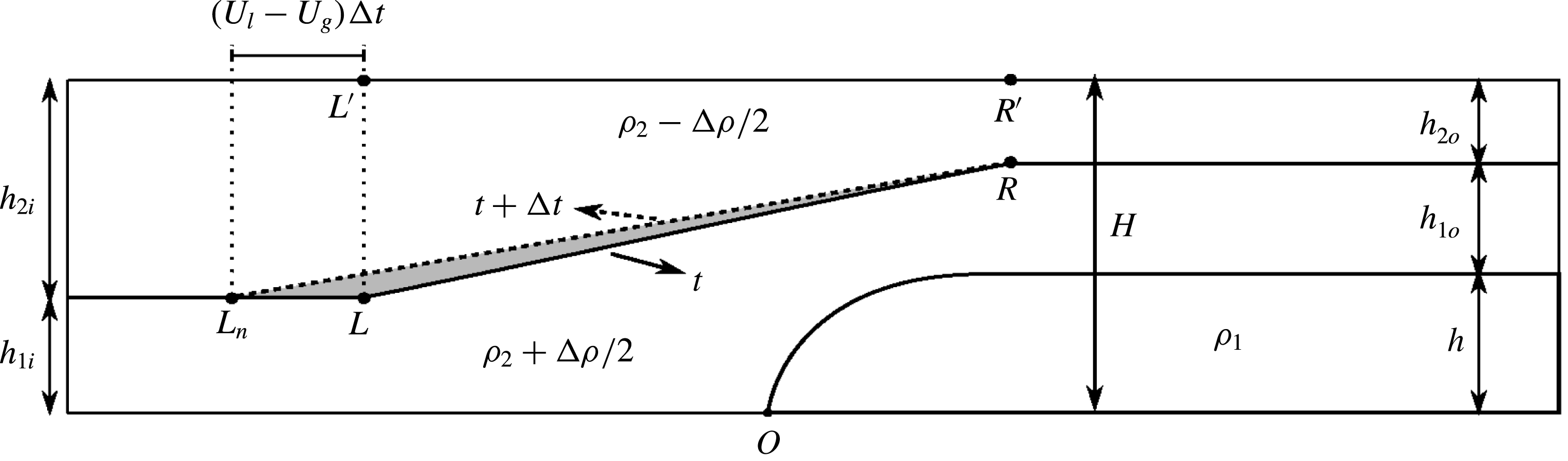
The propagation of the expansion wave furthermore lifts up the denser fluid of the lower layer, thereby increasing the potential energy. To quantify the rate of growth of potential energy, we analyse the evolution of the constant-slope interface over a small time interval
 $\unicode[STIX]{x0394}t$
, due to the propagation of the rarefaction wave, as shown in figure 10. The shaded region indicates the volume of light, upper layer fluid replaced by dense, lower layer fluid during
 $\unicode[STIX]{x0394}t$
. The rate at which the potential energy increases is then proportional to the rate at which the area of this triangle grows times the height of its centre of gravity, which results in
 $$\begin{eqnarray}{\dot{E}}_{p}^{\ast }=\frac{1}{2}\unicode[STIX]{x0394}\unicode[STIX]{x1D70C}^{\ast }(U_{l}^{\ast }-U_{g}^{\ast })(h^{\ast }+h_{1o}^{\ast }-h_{1i}^{\ast })\left(\frac{h^{\ast }+h_{1o}^{\ast }+2h_{1i}^{\ast }}{3}\right).\end{eqnarray}$$
The potential energy rate of growth can be added to the kinetic energy rate of growth to obtain
 ${\dot{E}}_{s}^{\ast }$
. We then substitute
 ${\dot{E}}_{s}^{\ast }$
into (3.32) to compute the rate of energy dissipation
 ${\dot{E}}_{d}^{\ast }$
.
Sketch in support of evaluating the unsteady potential energy term, in the reference frame moving with the gravity current. Over a small time interval
 $\unicode[STIX]{x0394}t$
, the left edge of the expansion wave travels from
 $L$
to
 $L_{n}$
with the constant velocity
 $U_{l}-U_{g}$
, while the right edge
 $R$
remains stationary. Within the expansion wave region, the interface is assumed to have a constant slope that changes with time. The shaded region indicates the volume of dense fluid of the lower layer that has replaced the light fluid of the upper layer during
 $\unicode[STIX]{x0394}t$
.

A corresponding analysis can be conducted for configuration C3 in order to obtain the rate of energy dissipation. Towards this end, we first compute the pressure drop along the top wall from (3.38), where the rate of accumulation of momentum
 ${\dot{M}}^{\ast }$
is now evaluated according to
 $$\begin{eqnarray}\displaystyle {\dot{M}}_{1}^{\ast } & = & \displaystyle \left[\frac{\text{d}}{\text{d}t^{\ast }}\int _{x_{l}^{\ast }}^{x_{r}^{\ast }}u_{1}^{\ast }(x^{\ast })d_{1}^{\ast }(x^{\ast })\,\text{d}x^{\ast }\right]+(U_{b}^{\ast }-U_{l}^{\ast })(U_{g}^{\ast }-U_{1b}^{\ast })h_{l}^{\ast }\nonumber\\ \displaystyle & & \displaystyle -\,(U_{b}^{\ast }-U_{g}^{\ast })U_{g}^{\ast }h_{1i}^{\ast },\end{eqnarray}$$
 $$\begin{eqnarray}\displaystyle {\dot{M}}_{2}^{\ast } & = & \displaystyle \left[\frac{\text{d}}{\text{d}t^{\ast }}\int _{x_{l}^{\ast }}^{x_{r}^{\ast }}u_{2}^{\ast }(x^{\ast })d_{2}^{\ast }(x^{\ast })\,\text{d}x^{\ast }\right]+(U_{b}^{\ast }-U_{l}^{\ast })(U_{g}^{\ast }+U_{2b}^{\ast })(1-h_{l}^{\ast })\nonumber\\ \displaystyle & & \displaystyle -\,(U_{b}^{\ast }-U_{g}^{\ast })U_{g}^{\ast }h_{2i}^{\ast }.\end{eqnarray}$$
The results of the above integrals can then be added up to obtain
 ${\dot{M}}^{\ast }$
for C3, which then enables us to compute
 $p_{3i}^{\ast }-p_{4o}^{\ast }$
from (3.38). In a corresponding fashion, we obtain
 $$\begin{eqnarray}\displaystyle {\dot{E}}_{k,1}^{\ast } & = & \displaystyle \left[\frac{\text{d}}{\text{d}t^{\ast }}\int _{x_{l}^{\ast }}^{x_{r}^{\ast }}\frac{1}{2}{u_{1}^{\ast }}^{2}(x^{\ast })d_{1}^{\ast }(x^{\ast })\,\text{d}x^{\ast }\right]+\frac{1}{2}(U_{b}^{\ast }-U_{l}^{\ast })(U_{g}^{\ast }-U_{1b}^{\ast })^{2}h_{l}^{\ast }\nonumber\\ \displaystyle & & \displaystyle -\,\frac{1}{2}(U_{b}^{\ast }-U_{g}^{\ast }){U_{g}^{\ast }}^{2}h_{1i}^{\ast },\end{eqnarray}$$
 $$\begin{eqnarray}\displaystyle {\dot{E}}_{k,2}^{\ast } & = & \displaystyle \left[\frac{\text{d}}{\text{d}t^{\ast }}\int _{x_{l}^{\ast }}^{x_{r}^{\ast }}\frac{1}{2}{u_{2}^{\ast }}^{2}(x^{\ast })d_{2}^{\ast }(x^{\ast })\,\text{d}x^{\ast }\right]+\frac{1}{2}(U_{b}^{\ast }-U_{l}^{\ast })(U_{g}^{\ast }+U_{2b}^{\ast })^{2}(1-h_{l}^{\ast })\nonumber\\ \displaystyle & & \displaystyle -\,\frac{1}{2}(U_{b}^{\ast }-U_{g}^{\ast }){U_{g}^{\ast }}^{2}h_{2i}^{\ast },\end{eqnarray}$$
and
 $$\begin{eqnarray}{\dot{E}}_{p}^{\ast }=\frac{1}{2}\unicode[STIX]{x0394}\unicode[STIX]{x1D70C}^{\ast }\left[(U_{l}^{\ast }-U_{g}^{\ast })(h^{\ast }+h_{1o}^{\ast }-h_{l}^{\ast })\frac{h^{\ast }+h_{1o}^{\ast }+2h_{l}^{\ast }}{3}+(U_{b}^{\ast }-U_{g}^{\ast })\frac{{h_{l}^{\ast }}^{2}-{h_{1i}^{\ast }}^{2}}{2}\right],\end{eqnarray}$$
so that we can evaluate the rate of energy dissipation
 ${\dot{E}}_{d}^{\ast }$
from (3.32).
4 Model predictions
In the following, we will discuss model predictions for the three configurations C1, C2 and C3. Towards this end, we solve the equations derived in § 3 via a MATLAB-based bisection root finding technique.
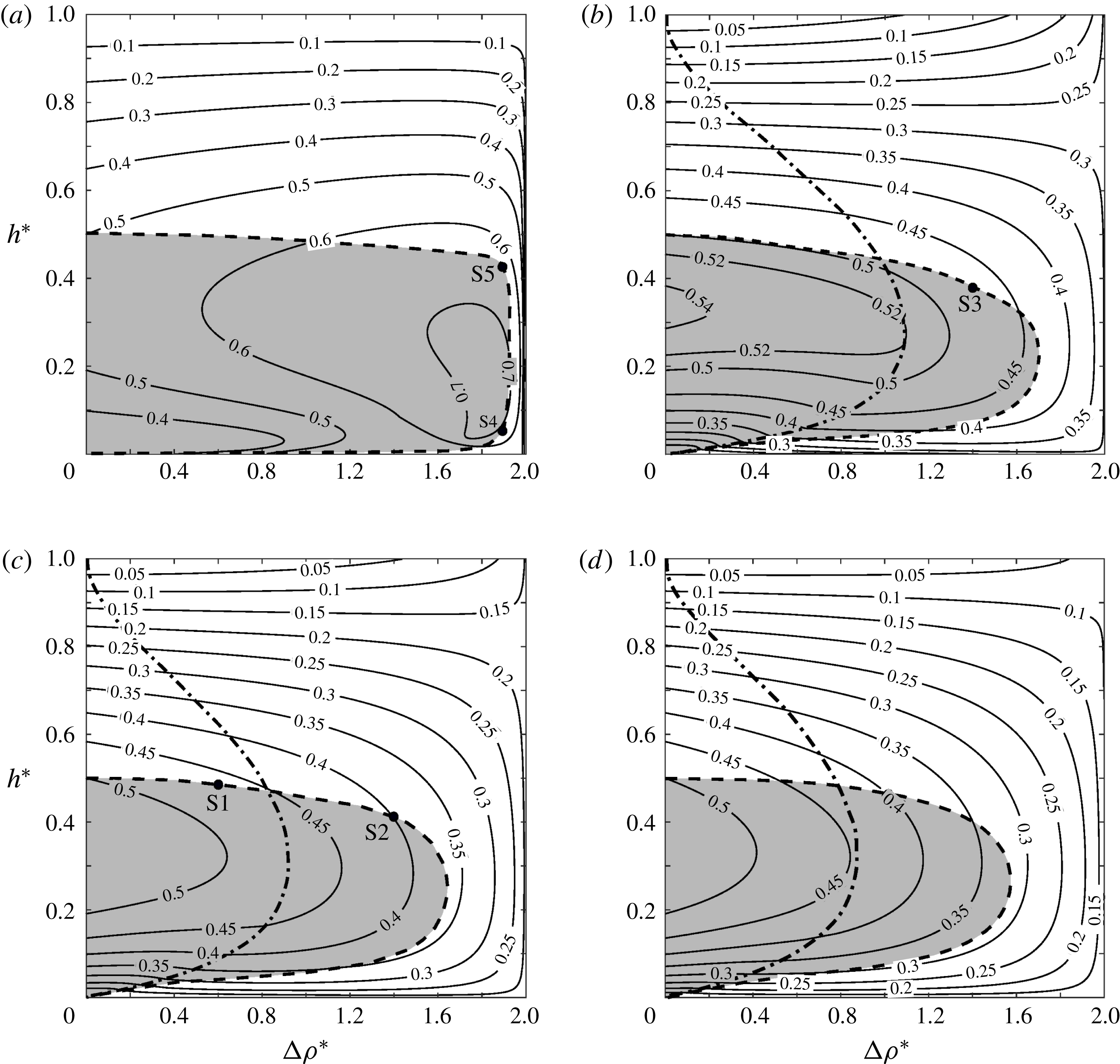
Phase-space diagrams for the gravity current velocity
 $U_{g}^{\ast }$
as function of the gravity current height
 $h^{\ast }$
and the stratification strength
 $\unicode[STIX]{x0394}\unicode[STIX]{x1D70C}^{\ast }$
. The interface heights at the inflow boundary are (a)
 $h_{1i}^{\ast }=0.05$
, (b)
 $h_{1i}^{\ast }=0.35$
, (c)
 $h_{1i}^{\ast }=0.50$
and (d)
 $h_{1i}^{\ast }=0.65$
. The shaded regions indicate solutions that are energetically possible. The dash-dotted lines distinguish steady C1-type solutions to the left from unsteady C2- and C3-type solutions to the right.

Figure 11 displays contours of the gravity current velocity
 $U_{g}^{\ast }$
for four different values of
 $h_{1i}^{\ast }$
, in the
 $\unicode[STIX]{x0394}\unicode[STIX]{x1D70C}^{\ast },h^{\ast }$
-plane. The shaded areas indicate the physically viable regions where the energy analysis of § 3.4 gives a positive energy dissipation rate
 $\dot{E_{d}}^{\ast }\geqslant 0$
. The outer boundary of the shaded region, marked by a dashed line, corresponds to energy-conserving solutions. The dash-dotted lines separate steady C1-type solutions to the left (
 $U_{g}^{\ast }\geqslant U_{l}^{\ast }$
), from unsteady C2- and C3-type flows with upstream-propagating waves (
 $U_{g}^{\ast }<U_{l}^{\ast }$
) to the right. The latter are based on the models of §§ 3.2 or 3.3, depending on whether
 $h_{1i}^{\ast }\geqslant 0.5$
or
 $h_{1i}^{\ast }<0.5$
. We find that without stratification (
 $\unicode[STIX]{x0394}\unicode[STIX]{x1D70C}^{\ast }=0$
), all values of
 $h_{1i}^{\ast }$
recover the classical result that half-depth gravity currents with
 $h^{\ast }=0.5$
are energy conserving and propagate with a velocity of 0.5 (Benjamin Reference Benjamin1968; Shin, Dalziel & Linden Reference Shin, Dalziel and Linden2004; Borden & Meiburg Reference Borden and Meiburg2013a
; Khodkar et al.
Reference Khodkar, Nasr-Azadani and Meiburg2017). We furthermore observe that for all inflow layer heights and stratification strengths, gravity currents with thickness greater than half the channel height cannot form without energy input.
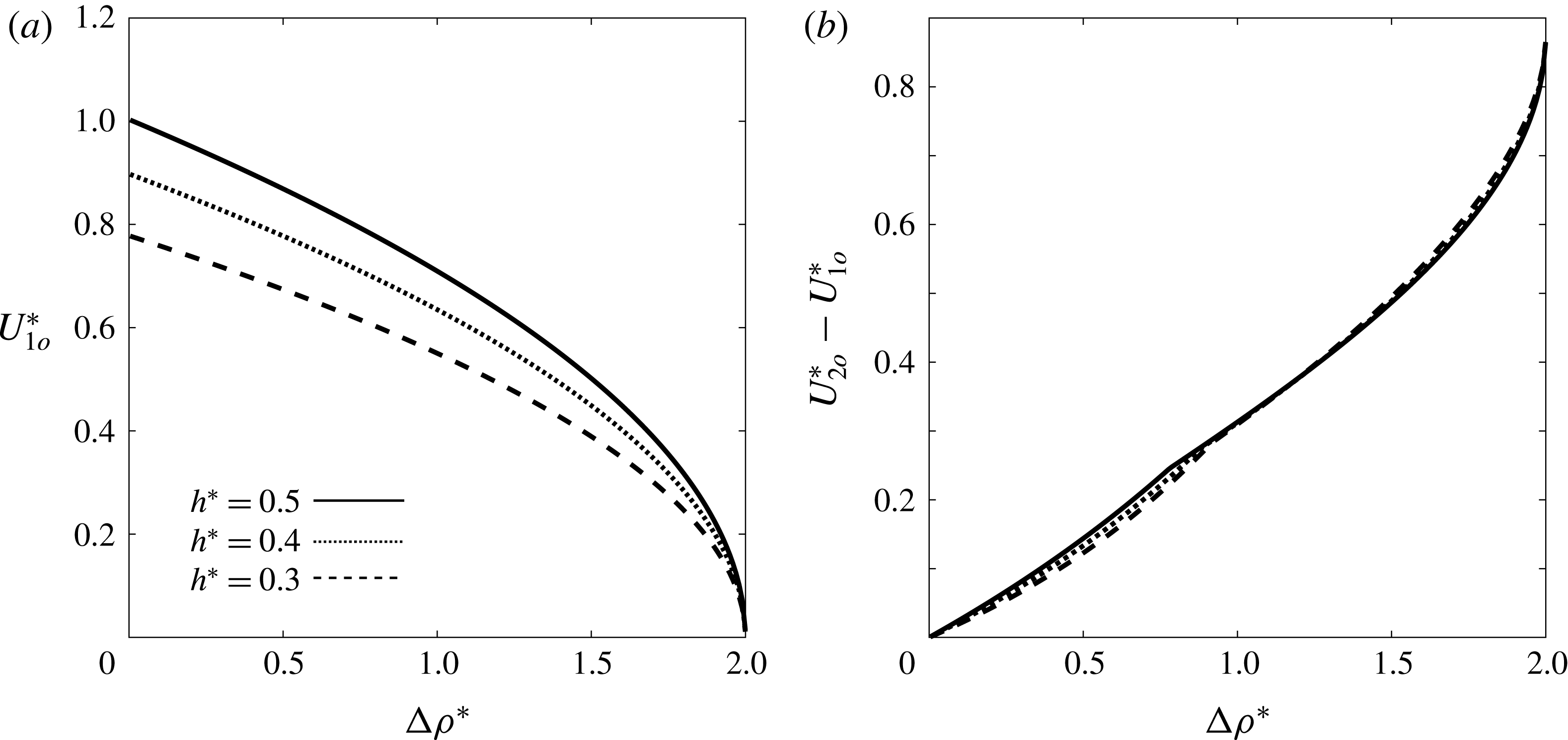
Figure 12 shows the outflow velocity
 $U_{1o}^{\ast }$
of the lower ambient layer, together with the shear across the ambient interface, as functions of the stratification parameter
 $\unicode[STIX]{x0394}\unicode[STIX]{x1D70C}^{\ast }$
, for several gravity current heights
 $h^{\ast }$
. In the limit of
 $\unicode[STIX]{x0394}\unicode[STIX]{x1D70C}^{\ast }\rightarrow 2$
, the density difference between the lower ambient layer and the gravity current vanishes, so that no vorticity is being generated along their boundary, and the lower ambient outflow velocity tends to zero. In this limit, the gravity current becomes indistinguishable from the lower ambient layer, so that we effectively recover the situation of a bore propagating along the interface between the ambient layers (Borden & Meiburg Reference Borden and Meiburg2013b
). Interestingly, for all density differences the shear across the interface between the ambient layers is nearly independent of the gravity current height.
The lower ambient outflow velocity
 $U_{1o}^{\ast }$
(a), and the outflow shear
 $U_{2o}^{\ast }-U_{1o}^{\ast }$
across the interface between the ambient layers (b), as functions of the stratification parameter
 $\unicode[STIX]{x0394}\unicode[STIX]{x1D70C}^{\ast }$
, for several gravity current heights
 $h^{\ast }$
. In all cases
 $h_{1i}^{\ast }=h_{2i}^{\ast }=0.5$
. In the limit
 $\unicode[STIX]{x0394}\unicode[STIX]{x1D70C}^{\ast }\rightarrow 2$
the flow reduces to a bore propagating along the interface between the ambient layers.

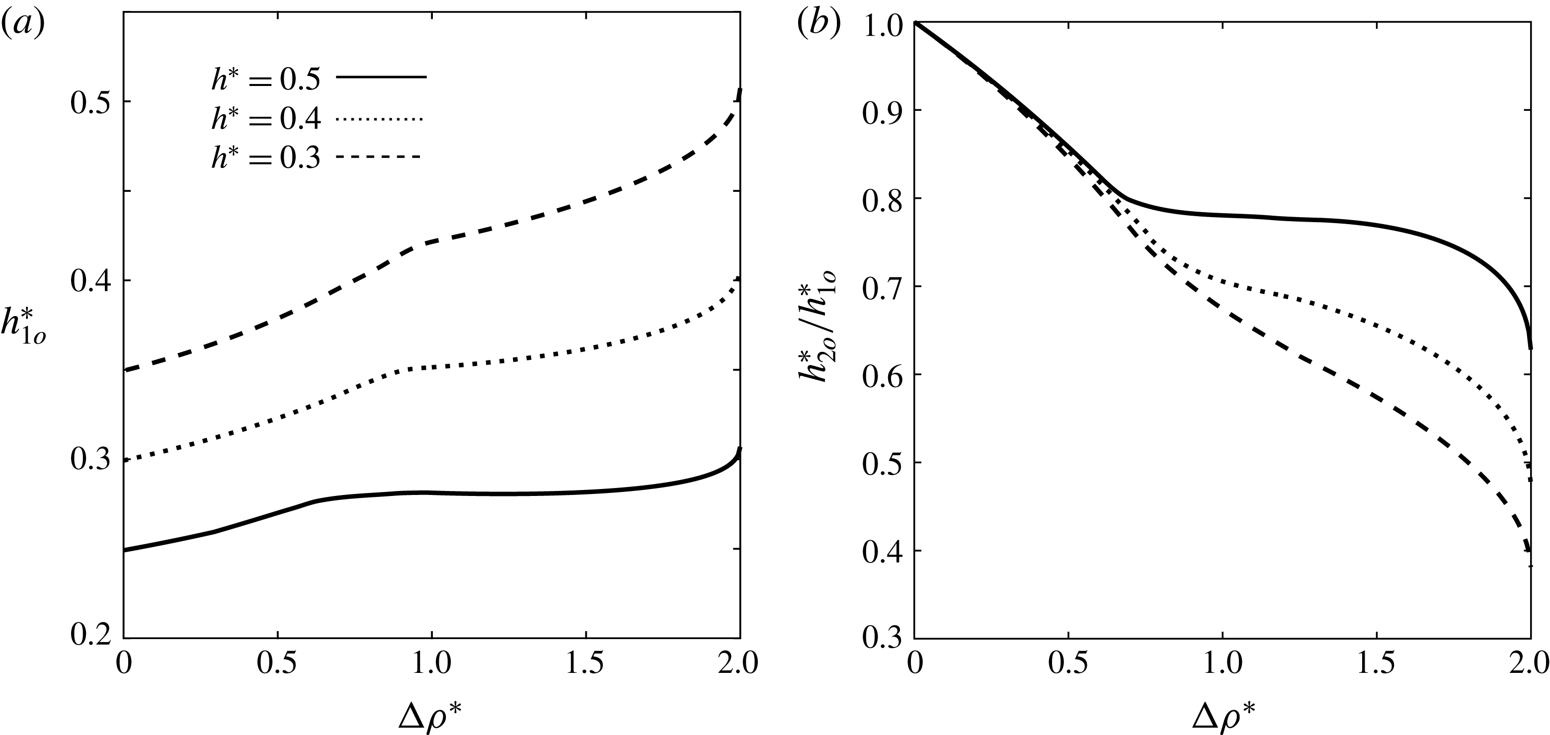
Figure 13(a) demonstrates that
 $h_{1o}^{\ast }$
grows with decreasing gravity current height, and that for a given gravity current height it increases monotonically with
 $\unicode[STIX]{x0394}\unicode[STIX]{x1D70C}^{\ast }$
. Figure 13(b) shows that the ratio
 $h_{2o}^{\ast }/h_{1o}^{\ast }$
decays monotonically with
 $\unicode[STIX]{x0394}\unicode[STIX]{x1D70C}^{\ast }$
. For small values of
 $\unicode[STIX]{x0394}\unicode[STIX]{x1D70C}^{\ast }$
, the dependence of
 $h_{2o}^{\ast }/h_{1o}^{\ast }$
on
 $h^{\ast }$
is quite weak. For larger values of
 $\unicode[STIX]{x0394}\unicode[STIX]{x1D70C}^{\ast }$
, when upstream-propagating disturbances emerge, the gravity current height has a substantial influence, so that smaller values of
 $h^{\ast }$
result in considerably smaller
 $h_{2o}^{\ast }/h_{1o}^{\ast }$
. We remark that in the limit of
 $\unicode[STIX]{x0394}\unicode[STIX]{x1D70C}^{\ast }\rightarrow 0$
, there will be no shear between the ambient layers at the outflow boundary: cf. (3.4) and figure 12(b). Hence, since the ambient layers are equally thick at the inflow, continuity requires that they also have the same thickness at the outflow. This is confirmed by the figure, which shows that
 $h_{2o}^{\ast }/h_{1o}^{\ast }\rightarrow 1$
as
 $\unicode[STIX]{x0394}\unicode[STIX]{x1D70C}^{\ast }\rightarrow 0$
.
The outflow thickness
 $h_{1o}^{\ast }$
of the lower ambient layer (a), and the ambient layer thickness ratio
 $h_{2o}^{\ast }/h_{1o}^{\ast }$
(b), as functions of the stratification parameter
 $\unicode[STIX]{x0394}\unicode[STIX]{x1D70C}^{\ast }$
, for several gravity current heights
 $h^{\ast }$
. In all cases
 $h_{1i}^{\ast }=h_{2i}^{\ast }=0.5$
.

Relationship between the flow regimes considered here for gravity currents propagating into two-layer stratified ambients, and those investigated by Rottman & Simpson (Reference Rottman and Simpson1989) in the context of two-layer stratified flows over solid obstacles. Shaded areas indicate energetically possible flows. The interface heights at the inflow boundary are (a)
 $h_{1i}^{\ast }=0.05$
, (b)
 $h_{1i}^{\ast }=0.35$
, (c)
 $h_{1i}^{\ast }=0.50$
and (d)
 $h_{1i}^{\ast }=0.65$
. Here, a, b, c and d represent supercritical, partially blocked, completely blocked and subcritical flow regimes, respectively, according to Rottman & Simpson (Reference Rottman and Simpson1989). a/b indicates the region in which both supercritical and partially blocked flows are plausible, depending on how the flow has been initiated. The dotted horizontal lines distinguish gravity current flows with upstream interfacial waves (below) from those without (above).

It is informative to relate the flow regimes considered in the present investigation of gravity currents propagating into two-layer stratified ambients, to those introduced by Rottman & Simpson (Reference Rottman and Simpson1989) for two-layer flows over solid topography. For four different values of
 $h_{1i}^{\ast }$
, figure 14 indicates energetically feasible gravity current flows by shaded regions in the
 $D_{o},F_{o}$
-plane, based on the analysis of § 3.4. We recall from § 1 that Rottman & Simpson (Reference Rottman and Simpson1989) define the Froude number
 $F_{o}=U_{g}^{\ast }/\sqrt{h_{1i}^{\ast }\unicode[STIX]{x0394}\unicode[STIX]{x1D70C}^{\ast }}$
, and the parameter
 $D_{o}=h^{\ast }/h_{1i}^{\ast }$
. Since gravity currents with thicknesses above half the channel depth would require an external energy input, no physically possible solution exists to the right of
 $D_{o}=0.5/h_{1i}^{\ast }$
. The horizontal dotted lines separate flows allowing for unsteady upstream disturbances (below), from those which are quasisteady in the gravity current reference frame (above). The figure suggests that for intermediate values of
 $h_{1i}^{\ast }$
partially blocked flows normally emerge, except when
 $F_{o}$
is relatively large. This situation can occur in two scenarios: (i) the gravity current velocity becomes very large, which usually is not the case for these values of
 $h_{1i}^{\ast }$
, since
 $U_{g}^{\ast }$
always remains below 0.55, or (ii)
 $\unicode[STIX]{x0394}\unicode[STIX]{x1D70C}^{\ast }\rightarrow 0$
. Alternatively, for small values of
 $h_{1i}^{\ast }$
supercritical flows can also appear when
 $\unicode[STIX]{x0394}\unicode[STIX]{x1D70C}^{\ast }$
is large, e.g.
 $\unicode[STIX]{x0394}\unicode[STIX]{x1D70C}^{\ast }=1.89$
in S4, since small values of
 $h_{1i}^{\ast }$
result in large Froude numbers. Consequently, the simulations of § 2 with moderate values of
 $h_{1i}^{\ast }$
all correspond to partially blocked flow. We note that partially blocked flows only result in upstream wave generation if the left edge of the wave travels faster than the gravity current head in the laboratory frame. The main distinction between supercritical and partially blocked flows is that the former never allow for the formation of upstream disturbances, whereas the latter may (S2 or S3) or may not (S1 and S5) lead to such disturbances, depending on whether
 $U_{g}^{\ast }<U_{l}^{\ast }$
or not, respectively. Those cases without upstream-propagating waves are located above the dotted lines along which
 $U_{g}^{\ast }=U_{l}^{\ast }$
, while those with upstream-propagating waves fall below these lines.
5 Comparison of model predictions and DNS simulation results
Table 2 compares predictions by the vorticity models of § 3 to DNS simulation results, for the specific flows discussed in § 2. These comparisons were carried out in the following fashion: for a given stratification parameter
 $\unicode[STIX]{x0394}\unicode[STIX]{x1D70C}^{\ast }$
and given ambient inflow layer heights, the DNS simulation was run until a quasisteady gravity current height
 $h^{\ast }$
was achieved. The values of
 $Re$
and
 $Pe$
in these simulations were chosen sufficiently large so that viscous and diffusive effects can be assumed small. For these values of
 $\unicode[STIX]{x0394}\unicode[STIX]{x1D70C}^{\ast }$
and
 $h^{\ast }$
, the gravity current velocity
 $U_{g}^{\ast }$
, the propagation speed
 $U_{l}^{\ast }$
of the expansion fan’s left edge (if applicable), and the outflow velocities and thicknesses of the ambient layers were then evaluated from the respective vorticity model, and compared to the corresponding DNS results. The subscript
 $n$
in the table refers to the DNS results, whereas the model predictions do not have subscripts. The model predictions and DNS results listed in the table are seen to agree with each other to within a few per cent. For simulation S3, the model predictions
 $h_{l}^{\ast }=0.5$
and
 $U_{b}^{\ast }=0.592$
for the internal bore properties (not listed in the table), while not quite as close, still agree reasonably well with the corresponding DNS results
 $h_{l,n}^{\ast }=0.448$
and
 $U_{b,n}^{\ast }=0.612$
.
Vorticity model predictions versus DNS results for the flows discussed in § 2.

The slight differences between the model predictions and DNS results can be partly attributed to the assumption of inviscid flow without diffusion underlying the models. The DNS simulations, on the other hand, have to employ finite values for
 $Re$
and
 $Pe$
, so that all interfaces have finite thicknesses. Furthermore, the momentum transfer between the flow layers as a result of viscosity causes an effective head gain in the ambient lower layer and the gravity current, which reduces the gravity current velocity in the simulations as compared to the model prediction. The presence of viscosity also leads to some dissipation throughout the flow. The quantitative influence of
 $Re$
and
 $Pe$
on the flow variables will be further discussed below. Finally, some of the discrepancy is due to the assumption that the interface height and vortex sheet strength vary linearly within the expansion wave region.
In all simulations, the gravity current height converged to a value near the boundary of the shaded region in figure 11, indicating that the evolving flow field in the simulations was always close to energy conserving for the given value of
 $\unicode[STIX]{x0394}\unicode[STIX]{x1D70C}^{\ast }$
and the prescribed inflow layer thicknesses. Hence, the specific vorticity model solution that conserves the overall energy of the flow usually provides a good prediction of the flow properties observed in the DNS. For this reason, we will refer to this energy-conserving model solution as ‘the vorticity model prediction’ in the following.
As shown in figure 11, for a given value of
 $\unicode[STIX]{x0394}\unicode[STIX]{x1D70C}^{\ast }$
there are generally two energy-conserving solutions for the gravity current height: one located on the upper branch, and other located on the lower branch of the boundary between the shaded and unshaded regions. Multiple energy-conserving solutions were also found by Holyer & Huppert (Reference Holyer and Huppert1980) and White & Helfrich (Reference White and Helfrich2012). Holyer & Huppert (Reference Holyer and Huppert1980) state that the current chooses the solution maximizing its volumetric inflow rate (
 $U_{g}^{\ast }h^{\ast }$
), which always corresponds to the one with the largest
 $h^{\ast }$
-value. We observed a similar tendency in our DNS simulations, in that for moderate values of
 $h_{1i}^{\ast }\gtrsim 0.15$
the gravity current usually thickened and converged to the upper solution, even when initialized close to the lower branch. For very small values of
 $h_{1i}^{\ast }$
, on the other hand, the DNS simulations converged to two different gravity current heights, depending on the initialization, as shown in figure 9.
5.1 Influence of dimensionless parameters
As stated earlier, in the analytical models presented in § 3, the fluids are assumed to be inviscid and the interfaces are considered sharp, so that no diffusive momentum or mass transfer can occur between the different flow layers. On the other hand, the DNS simulations of § 2 employ finite Reynolds and Péclet numbers, so that momentum and scalar interfaces have finite thicknesses. Here we investigate the quantitative influence of the
 $Re$
- and
 $Pe$
-values on the DNS results.
Influence of the Reynolds number on the downstream density (a), and velocity (b) profiles across the channel height, for simulation S1 shown in figure 4.
 $Pe$
is held fixed at 20 000. The straight dashed lines represent the model predictions of § 3. As
 $Re$
increases, the agreement between model predictions and simulation results generally improves.

Influence of the Péclet number on the downstream density (a), and velocity (b) profiles across the channel height, for simulation S1 shown in figure 4.
 $Re$
is held fixed at 5000. The straight dashed lines represent the model predictions of § 3. As
 $Pe$
increases, the agreement between model predictions and simulation results generally improves.

For simulation S1, figures 15 and 16 display the vertical density and velocity profiles far downstream of the gravity current front, at
 $x^{\ast }=0.9L_{x}$
. Note that in all simulations of figure 15,
 $Pe=20\,000$
, and in those of figure 16,
 $Re=5000$
. While the model assumes that the velocity inside the gravity current vanishes in the reference frame moving with the gravity current front, the DNS simulations show that the gravity current fluid moves towards the front near the bottom wall, and away from it near the upper interface, as a result of the finite
 $Re$
- and
 $Pe$
-values. The agreement between the model predictions and DNS results improves for larger
 $Re$
- and
 $Pe$
-values, as viscous and diffusive effects diminish. Similarly, the velocity gradients in the interfacial regions approach the step-like model profiles for larger
 $Re$
and
 $Pe$
. Corresponding observations can be made regarding the density profiles, in that they become more step-like and closer to the model predictions as
 $Re$
and
 $Pe$
increase. The influence of
 $Re$
on the density profiles is relatively small, however. We note that as
 $Re$
is increased beyond approximately 6000, the agreement between model predictions and DNS results will no longer improve, due to the appearance of unsteady Kelvin–Helmholtz vortices.
6 Comparison with earlier models
We now proceed to compare predictions by the current vorticity-based models to those of previous models by other authors. Figure 17 provides comparison data for the gravity current height
 $h^{\ast }$
and velocity
 $U_{g}^{\ast }$
as functions of the density jump
 $\unicode[STIX]{x0394}\unicode[STIX]{x1D70C}^{\ast }$
, for
 $h_{1i}^{\ast }=0.5$
. We note that the models of Holyer & Huppert (Reference Holyer and Huppert1980) and Tan et al. (Reference Tan, Nobes, Fleck and Flynn2010) solve for the gravity current height, while the model by White & Helfrich (Reference White and Helfrich2012) solves for the other flow parameters as a function of the gravity current height. Hence, for that model figure 17 shows the specific solution for which energy is conserved. Similarly, as discussed above, we take as the vorticity model prediction the energy-conserving solution. As shown in § 3.1, when the flow does not give rise to upstream waves and configuration C1 applies, vorticity conservation implies that the head loss in both ambient layers is identical, consistent with the assumption made by White & Helfrich (Reference White and Helfrich2012). On the other hand, when upstream propagating disturbances in the form of an expansion wave or an internal bore followed by a rarefaction wave appear, overall energy conservation implies that an energy gain in one layer corresponds to an energy loss in the other one. According to figure 17, for
 $h_{1i}^{\ast }=0.5$
the model of White & Helfrich (Reference White and Helfrich2012) predicts that no energy-conserving flows form for
 $\unicode[STIX]{x0394}\unicode[STIX]{x1D70C}^{\ast }>1.16$
, while the corresponding value for the vorticity model is 1.64.
Comparison of current and previous model predictions for (a) the gravity current height, and (b) the gravity current velocity, as function of
 $\unicode[STIX]{x0394}\unicode[STIX]{x1D70C}^{\ast }$
and for
 $h_{1i}^{\ast }=0.5$
. Here, those solutions from White & Helfrich (Reference White and Helfrich2012) and the current investigation are shown that conserve energy. The vertical solid line indicates the transition from C1 to C2 according to the vorticity model, while the vertical dashed line represents the largest value of
 $\unicode[STIX]{x0394}\unicode[STIX]{x1D70C}^{\ast }$
for which the conjugate flow theory of White & Helfrich (Reference White and Helfrich2012) predicts an energy-conserving solution. To the left of the dashed line, Holyer & Huppert (Reference Holyer and Huppert1980) and White & Helfrich (Reference White and Helfrich2012) render identical predictions. For supercritical gravity currents, both of these solutions are identical to the vorticity model. The corresponding DNS results are indicated by S1 and S2.

Figure 17 shows that all models reproduce the classical solution
 $h^{\ast }=0.5$
and
 $U_{g}^{\ast }=0.5$
of Benjamin (Reference Benjamin1968) for gravity currents without ambient stratification. Furthermore, for configuration C1 the predictions by Holyer & Huppert (Reference Holyer and Huppert1980), White & Helfrich (Reference White and Helfrich2012) and the vorticity model are identical. When upstream rarefaction waves arise for
 $\unicode[STIX]{x0394}\unicode[STIX]{x1D70C}^{\ast }>0.83$
, the predictions of the vorticity model deviate from those of Holyer & Huppert (Reference Holyer and Huppert1980) and White & Helfrich (Reference White and Helfrich2012), which do not account for this feature.
The two models of Tan et al. (Reference Tan, Nobes, Fleck and Flynn2010) invoke an empirical argument concerning the magnitude of the ambient interface deflection, as expressed by (1.1), and as a result their predictions for the height and velocity of the gravity current differ from the other models. Figure 18 compares this empirical assumption by Tan et al. (Reference Tan, Nobes, Fleck and Flynn2010) for the outflow thickness of the upper ambient layer with the corresponding prediction by the vorticity model, as well as with DNS results. While the predictions of the two models are clearly distinct, the quantitative difference is always less than ten per cent. The two DNS results are seen to agree more closely with the vorticity model prediction.
Predictions by the model of Tan et al. (Reference Tan, Nobes, Fleck and Flynn2010) and by the vorticity model for the outflow thickness of the upper ambient layer as a function of
 $\unicode[STIX]{x0394}\unicode[STIX]{x1D70C}^{\ast }$
, for
 $h_{1i}^{\ast }=0.5$
. The corresponding DNS results are indicated by S1 and S2. Configuration C1 exists to the left of the vertical dotted line.

Interestingly, the models of Holyer & Huppert (Reference Holyer and Huppert1980) and Tan et al. (Reference Tan, Nobes, Fleck and Flynn2010) break down for
 $\unicode[STIX]{x0394}\unicode[STIX]{x1D70C}^{\ast }>1.2$
, independent of the
 $h_{1i}^{\ast }$
-value. Tan et al. (Reference Tan, Nobes, Fleck and Flynn2010) suggest that this degeneration may be due to the formation of upstream waves, which are neglected in both studies. As a possible alternative, they speculate that the head loss in the dissipative ambient layer becomes negative when
 $\unicode[STIX]{x0394}\unicode[STIX]{x1D70C}^{\ast }>1.2$
. Tan et al. (Reference Tan, Nobes, Fleck and Flynn2010) furthermore suggest that the transition from the internal bore to the expansion fan occurs when
 $h_{1i}^{\ast }\gtrsim 0.3$
. On the other hand and consistent with the findings of Baines (Reference Baines1984) and Lawrence (Reference Lawrence1993), the vorticity model predicts the transition from C3 to C2 to occur when the bore reaches its maximum amplitude, or equivalently when
 $h_{1i}^{\ast }>0.5$
. Equivalently, White & Helfrich (Reference White and Helfrich2012) find the boundaries between the two regimes when the flow immediately upstream of the gravity current becomes critical.
Figure 17 shows only the conjugate flow solution of White & Helfrich (Reference White and Helfrich2012) for steady-state gravity currents with no upstream-propagating disturbances. As mentioned in the introduction, White & Helfrich (Reference White and Helfrich2012) also propose an alternative model which accounts for a left-propagating internal bore (but not for an expansion fan), as sketched in figure 2. For this model, White & Helfrich (Reference White and Helfrich2012) assume energy conservation downstream of the bore and within the gravity current region (
 $1b-1o-4o-3b$
). The range of validity of this bore-inclusive model is given by their equations (2.11) and (2.12). According to those equations, S3 and other DNS simulations of the present study with an upstream rarefaction wave and internal bore fall outside the range of validity of the bore-inclusive model by White & Helfrich (Reference White and Helfrich2012), so that we cannot undertake a direct comparison.
7 Conclusions
We have extended the vorticity-based modelling approach originally introduced by Borden & Meiburg (Reference Borden and Meiburg2013a ,Reference Borden and Meiburg b ) to gravity currents propagating into two-layer stratified ambients. Towards this end, we have developed vorticity-based models for three different flow configurations, viz. no upstream-propagating wave (C1), an upstream-propagating expansion wave only (C2), an upstream-propagating expansion wave and a bore (C3). Configuration C1 is quasisteady in the reference frame moving with the gravity current, and it does not require any empirical closure assumptions. Configurations C2 and C3, on the other hand, are unsteady even in the moving reference frame, and in order to obtain a closed system of equations we assume that certain flow properties vary linearly along the unsteady expansion fan. If we prescribe the gravity current height and the stratification strength along with the ambient inflow layer thicknesses and velocities, the models yield the gravity current velocity, the bore and expansion wave properties, as well as the ambient outflow layer thicknesses and velocities. Furthermore, the model equations provide information as to which of the three configurations will occur in a given parameter regime.
Since we do not require energy-related closure assumptions for any of the configurations, the energetics of the different flow fields can be analysed a posteriori, after the full flow field has been determined. In this way, we can determine the dissipation associated with each gravity current height, for a given set of flow parameters. In order to determine which gravity current height will be selected in Navier–Stokes flows, we then conduct two-dimensional DNS simulations that can be compared to the model results. These simulations yield gravity current heights in close agreement with the vorticity model solutions for energy-conserving flows, so that we adopt this energy-conserving solution as the vorticity model prediction. For the quasisteady C1 configuration, the vorticity model predictions agree with the earlier models by Holyer & Huppert (Reference Holyer and Huppert1980) and White & Helfrich (Reference White and Helfrich2012), and with the DNS simulations. In the presence of an expansion fan, however, only the vorticity model predictions are close to the DNS results.
We furthermore discuss some of the differences between the present flow regimes for gravity currents propagating into two-layer stratified ambients, and earlier analyses of two-layer stratified flows over solid topography. Interestingly, the gravity current simulations do not indicate the presence of a completely blocked flow regime, whose existence is well established for flow over solid topography.
Acknowledgements
The authors gratefully acknowledge support through NSF grant no. CBET-1335148.