1 Introduction
It is not uncommon that rough surfaces with significant variation in the roughness height occur in engineering and environmental flows. Examples include gas turbine blades, atmospheric boundary layers, and ship hulls. Idealizations of such non-equilibrium, rough-wall turbulent flows have been investigated by laboratory experiments (Antonia & Luxton Reference Antonia and Luxton1971, Reference Antonia and Luxton1972; Pearson, Elavarasan & Antonia Reference Pearson, Elavarasan and Antonia1997; Cheng & Castro Reference Cheng and Castro2002; Jacobi & Mckeon Reference Jacobi and Mckeon2011). Particularly relevant to the present work, Antonia & Luxton (Reference Antonia and Luxton1972), Taylor et al. (Reference Taylor, Taylor, Hosni and Coleman1993) and Hanson & Ganapathisubramani (Reference Hanson and Ganapathisubramani2016) studied the relaxation of fully developed, rough-wall turbulent boundary layers towards fully developed smooth-wall states, on encountering a sudden change in boundary condition, from rough to smooth (RTS). RTS flows form a subset of more general non-equilibrium rough-wall flows, and are the subject of numerical experiments presented herein. Despite the obvious importance in understanding rough-to-smooth evolution, to the best of our knowledge, there have been no previous, fully resolved, numerical simulations of RTS flows.
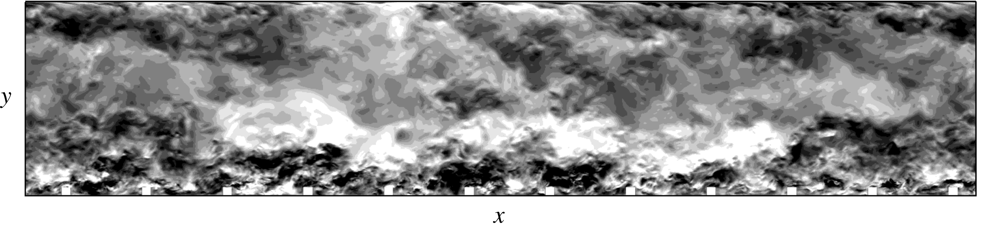
Many high-Reynolds-number turbulent flows of engineering significance are, in essence, hydrodynamically rough. For such flows, the viscous sublayer and buffer layer, that are encountered on smooth walls, are replaced by a roughness sublayer which extends above the surface to between two and five times the roughness height (Raupach, Antonia & Rajagopalan Reference Raupach, Antonia and Rajagopalan1991). Within this roughness sublayer, in addition to intensification of turbulence, the large-scale structure is enhanced and shows strong interaction with the overlying outer flow. The high-intensity turbulence in this sublayer transfers momentum between the surface and the outer regions – as is clear from the instantaneous streamwise velocity fluctuations,
 $u^{\prime }$
, of a rib-roughened, fully developed turbulent flow in figure 1. Inside the roughness cavities in figure 1, turbulence is characterized by three-dimensional unstable eddies with size of the order of the roughness height (Ikeda & Durbin Reference Ikeda and Durbin2007), which is typical of
 $k$
-type rough-wall flows (Perry, Schofield & Joubert Reference Perry, Schofield and Joubert1969).
In RTS flows, the rough-wall structure carries downstream over the smooth wall. The skin friction shows a sharp reduction, as the drag of roughness elements is removed, but followed by a quick recovery towards equilibrium smooth-wall levels. This is accompanied by a comparatively slow recovery of the mean velocity towards the smooth-wall values. This behaviour has been seen in RTS lab experiments; in Antonia & Luxton (Reference Antonia and Luxton1972), profiles of both mean velocity and turbulence stresses showed incomplete relaxation by the last measuring station, located at approximately 16 boundary-layer thicknesses downstream of the step change. These authors argued that this slow recovery is a feature of both inner and outer layers. Although they were able to fit conventional log-laws to the mean-velocity profiles on the developing smooth wall, the intercept was considerably higher than the fully developed, smooth-wall value of approximately 5.1. The present simulations show that the log-law is not established, at all, in the recovery region.
Instantaneous streamwise velocity fluctuations,
 $u^{\prime }$
, in the
 $xy$
-plane for a fully developed, rough-wall turbulent channel flow. Scale: white
 $+0.2$
, black
 $-0.2$
.

More recently, Hanson & Ganapathisubramani (Reference Hanson and Ganapathisubramani2016), in their RTS boundary-layer experiments, with mesh-type and grit-type roughnesses, showed virtually complete recovery of mean-velocity profiles, but the streamwise turbulence stresses remained higher than equilibrium all the way to the last measuring station. Hanson & Ganapathisubramani (Reference Hanson and Ganapathisubramani2016) proposed the internal boundary height as an appropriate length scale in the transitional regime. The internal boundary-layer height was meant to discriminate between a region influenced by the new boundary condition, and an overlying region that is primarily determined by the upstream rough wall. However, except for tracking the outer peaks of streamwise turbulence stress, and providing a gross demarcation between the two aforementioned regions, the utility of this internal layer concept was rather limited.
The present study aims to contribute to the existing literature on non-equilibrium RTS turbulent flows by (i) being the first, fully resolved computer simulations of transition from a fully developed rough-wall state to the developing smooth-wall behaviour in turbulent channel flows, highlighting the non-equilibrium turbulent flow development; (ii) providing an accurate estimation of skin-friction levels, which are difficult to measure by experimental techniques (see Jacobi & Mckeon Reference Jacobi and Mckeon2011); (iii) examining the transitional behaviour of the turbulent flow, by systematically varying the downstream viscous and the upstream roughness length scales; (iv) elaborating on the existing statistical picture of similar turbulent flows, as painted by laboratory experiments, using turbulence stresses, quadrant analysis and energy spectra; and (v) visualizing instantaneous fluctuating flow fields to complement these statistical measures.
2 Simulation preliminaries
The incompressible Navier–Stokes equations,
 $$\begin{eqnarray}\displaystyle & \displaystyle \frac{\unicode[STIX]{x2202}u_{i}}{\unicode[STIX]{x2202}x_{i}}=0, & \displaystyle\end{eqnarray}$$
 $$\begin{eqnarray}\displaystyle & \displaystyle \frac{\unicode[STIX]{x2202}u_{i}}{\unicode[STIX]{x2202}t}+\frac{\unicode[STIX]{x2202}u_{i}u_{j}}{\unicode[STIX]{x2202}x_{j}}=-\frac{1}{\unicode[STIX]{x1D70C}}\frac{\unicode[STIX]{x2202}p}{\unicode[STIX]{x2202}x_{i}}+\unicode[STIX]{x1D708}\frac{\unicode[STIX]{x2202}^{2}u_{i}}{\unicode[STIX]{x2202}x_{j}^{2}}, & \displaystyle\end{eqnarray}$$
are solved by the fractional time-step method described in Pierce & Moin (Reference Pierce and Moin2004). In (2.2)
 $u_{i}=\{U,V,W\}$
are the instantaneous velocities in the streamwise, wall-normal and spanwise directions (
 $x,y,z$
), respectively,
 $p$
is the pressure and
 $\unicode[STIX]{x1D708}$
is the kinematic viscosity. In this study, the superscript
 $^{\prime }$
is used to identify the fluctuating component and an over-bar will be used to signify the mean value of various turbulence statistics. The algorithm employs finite differences on a three-dimensional, staggered, Cartesian mesh. Second-order central differences are used for all spatial derivatives. The discrete equations are advanced in time by a semi-implicit scheme based on Newton–Raphson iterations, which is second-order accurate.
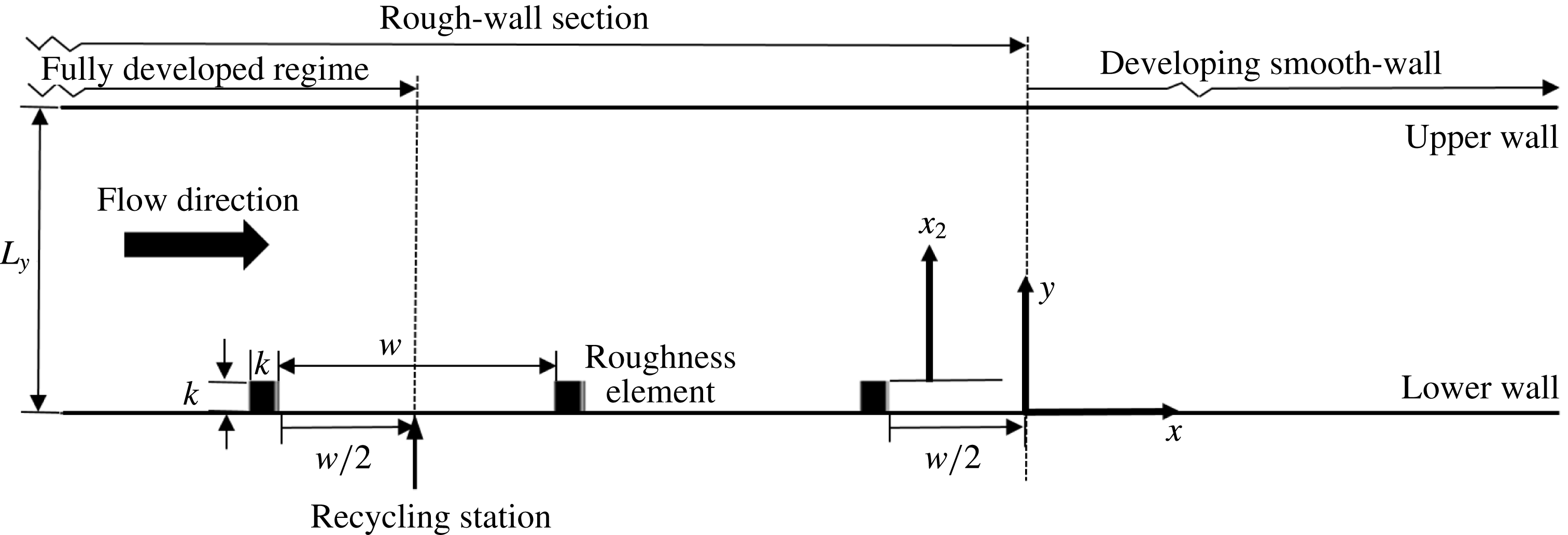
Computational domain and coordinate system. Spanwise (
 $z$
) direction is outward from the figure.

The computational domain is divided into two sections: an initial rough-wall section of length
 $L_{rs}$
is followed by a smooth-wall section. A schematic is provided in figure 2. Square cylindrical ribs of height
 $k$
are placed on the bottom, rough wall, while the upper wall is kept smooth. The geometry of the rough wall is similar to the fully developed rough-wall simulations by Ikeda & Durbin (Reference Ikeda and Durbin2002, Reference Ikeda and Durbin2007) and Leonardi et al. (Reference Leonardi, Orlandi, Smalley, Djenidi and Antonia2003). Following Ikeda & Durbin (Reference Ikeda and Durbin2007), the spacing between successive roughness elements is
 $w/k=9$
. This spacing is sufficiently wide to ensure
 $k$
-type roughness, while providing near-maximum form drag. A recycling plane is used to generate a fully developed rough wall in the initial section, of length
 $L_{fdr}$
, and to establish realistic turbulent inflow conditions for the smooth section. This recycling plane can, alternatively, be thought of as the inflow plane for the subsequent, downstream developing, channel flow. The procedure involves extracting an instantaneous cross-flow plane of the velocity field at the streamwise recycling station and applying it at the inflow. The inflow mass-flow rate is maintained constant at every time step.
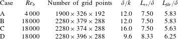
Four test cases have been simulated, all of which have identical streamwise and wall-normal extents of the domain, which are
 $L_{x}=15.83\unicode[STIX]{x1D6FF}$
and
 $L_{y}=2.00\unicode[STIX]{x1D6FF}$
. The spanwise domain size for the low-Reynolds-number case is
 $L_{z}=1.96\unicode[STIX]{x1D6FF}$
, and for the high-Reynolds-number cases
 $L_{z}=2.08\unicode[STIX]{x1D6FF}$
. Additional parameters are summarized in table 1. These test cases are primarily differentiated by their
 $\unicode[STIX]{x1D6FF}/k$
ratio and by their bulk Reynolds number,
 $Re_{b}=U_{b}\unicode[STIX]{x1D6FF}/\unicode[STIX]{x1D708}$
, where
 $U_{b}$
is the bulk velocity.
The initial, fully developed, rough-wall regime includes enough roughness elements within its length,
 $L_{fdr}$
, for the near-wall, streamwise two-point correlations to become low at large streamwise separations. Leonardi et al. (Reference Leonardi, Orlandi, Smalley, Djenidi and Antonia2003) and Ikeda & Durbin (Reference Ikeda and Durbin2007) both had four roughness elements for their fully developed rough-wall simulations, which is around half the number we have used for any of our test cases. Two roughness cavities after the recycling station were found adequate to provide a short, yet naturally developing evolution between the initial fully developed rough-wall regime and the developing, smooth-wall regime. The difference in the mean reattachment lengths of the primary recirculation region between the last roughness element and a roughness element in the fully developed, rough-wall regime was approximately
 $5\,\%$
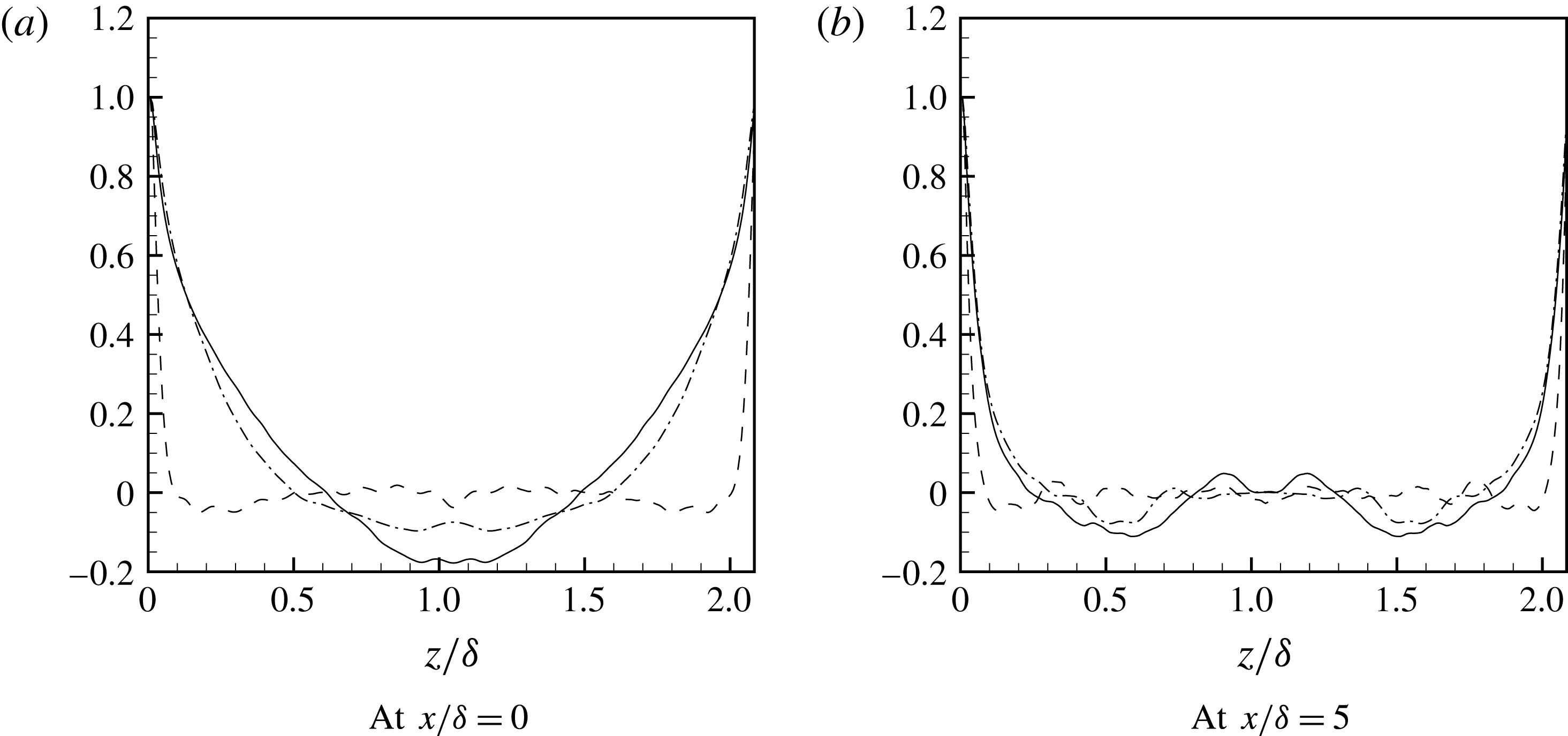
. The spanwise domain is sufficiently wide to avoid spurious correlation in that direction. Figure 3, for case B, shows the normalized two-point correlations of the fluctuating velocities,
 $$\begin{eqnarray}\displaystyle & \displaystyle R_{\unicode[STIX]{x1D6FC}\unicode[STIX]{x1D6FC}}^{z}(x,z)=\frac{\overline{\unicode[STIX]{x1D6FC}^{\prime }(x,z)\unicode[STIX]{x1D6FC}^{\prime }(x,z+\unicode[STIX]{x0394}z)}}{\overline{\unicode[STIX]{x1D6FC}^{\prime }\unicode[STIX]{x1D6FC}^{\prime }}}, & \displaystyle\end{eqnarray}$$
where
 $\unicode[STIX]{x1D6FC}=(u,v,w)$
. The two figures are in the near-wall region, at the centre of a cavity in the fully developed rough-wall region, and at
 $x/\unicode[STIX]{x1D6FF}=5.0$
in the developing, smooth-wall region. The drop of these two-point correlations to levels close to zero indicates that the spanwise domain size is adequate.
Two-point correlations of fluctuating velocities in the spanwise direction at
 $y/\unicode[STIX]{x1D6FF}=0.060$
for case B. ——
 $R_{uu}^{z}$
, – – –
 $R_{vv}^{z}$
and – ⋅ – ⋅ –
 $R_{ww}^{z}$
.

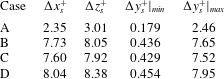
Summary of simulation parameters.

Jimnez (Reference Jimnez2004) recommended a
 $\unicode[STIX]{x1D6FF}_{b}/k>40$
for similarity laws to appear in turbulent rough-wall boundary layers, where
 $\unicode[STIX]{x1D6FF}_{b}$
is the 99 % boundary-layer thickness. Many earlier laboratory experiments and direct simulations have used smaller values (e.g. Cheng & Castro Reference Cheng and Castro2002; Orlandi, Leonardi & Antonia Reference Orlandi, Leonardi and Antonia2006; Ikeda & Durbin Reference Ikeda and Durbin2007). Some recent physical experiments have exceeded the criterion (e.g. Volino, Schultz & Flack Reference Volino, Schultz and Flack2011; Squire et al.
Reference Squire, Morrill-Winter, Hutchins, Schultz, Klewicki and Marusic2016). Here, we assume the channel half-height
 $\unicode[STIX]{x1D6FF}$
and
 $\unicode[STIX]{x1D6FF}_{b}$
are equivalent. For their square-rib simulations Miyake, Tsujimoto & Nagai (Reference Miyake, Tsujimoto and Nagai2002) and Leonardi et al. (Reference Leonardi, Orlandi, Smalley, Djenidi and Antonia2003) used
 $\unicode[STIX]{x1D6FF}/k=5$
, while Ikeda & Durbin (Reference Ikeda and Durbin2007) used
 $\unicode[STIX]{x1D6FF}/k=8.5$
. Ashrafian, Andersson & Manhart (Reference Ashrafian, Andersson and Manhart2004) used a higher ratio of
 $\unicode[STIX]{x1D6FF}/k\approx 30$
, but their simulations were only transitionally rough. Nagano, Hattori & Houra (Reference Nagano, Hattori and Houra2004) used three different ratios,
 $\unicode[STIX]{x1D6FF}/k=5,10$
and
 $20$
. Although they did not directly report their effective sand-grain length scales, by using the reported
 $k^{+}$
we infer that
 $\unicode[STIX]{x1D6FF}/k=20$
, and that the flow was transitionally rough. It should be noted that a higher
 $\unicode[STIX]{x1D6FF}/k$
, although desirable, reduces the effective sand grain roughness
 $r^{+}$
for a given bulk Reynolds number,
 $Re_{b}$
. The present choices of
 $\unicode[STIX]{x1D6FF}/k=9.6,12$
and
 $16$
, are larger than those used by most previous DNS studies, and ensure that the rough wall falls in the fully rough regime, i.e
 $r^{+}>90$
(see Durbin & Reif Reference Durbin and Reif2011). In this fully rough category, if the roughness geometry is fixed, the flow becomes independent of
 $\unicode[STIX]{x1D708}$
; or, the friction velocity on the rough wall
 $u_{\unicode[STIX]{x1D70F}R}$
becomes independent of
 $Re_{b}$
.
Spatial and temporal resolutions for the RTS cases. The normalization is with the friction velocity at the upper smooth wall in the fully developed rough-wall region,
 $u_{\unicode[STIX]{x1D70F}S}$
.
Approximate maxima of local grid spacing normalized by the local Kolmogorov length scale
 $\unicode[STIX]{x1D702}=(\unicode[STIX]{x1D708}^{3}/\unicode[STIX]{x1D716})^{0.25}$
for the RTS cases.

Following Antonia & Luxton (Reference Antonia and Luxton1972), the start of the developing, smooth-wall regime (
 $x=0$
) is located at a distance
 $w/2$
after the last roughness element. This origin is located downstream of the primary recirculation zone following the last roughness element. Also such a choice means that the rough-wall section has an integer number of roughness cavities of equal size. For each roughness cavity the skin friction is calculated using both form drag and viscous drag, whereas in the developing smooth-wall section skin friction is simply the viscous drag.
The no-slip condition is applied on the upper and lower walls. Periodic boundary conditions are used in the spanwise direction and the convective outflow condition
 $\unicode[STIX]{x2202}u_{i}/\unicode[STIX]{x2202}t+c\unicode[STIX]{x2202}u_{i}/\unicode[STIX]{x2202}x=0$
is applied at the outlet boundary, where
 $c$
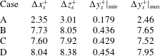
is the local bulk velocity. Uniform grid spacing is used in the streamwise and spanwise directions, while a non-uniform grid is used in the wall-normal direction, with mesh clustering near the bottom wall, near the top of the roughness elements and near the upper smooth wall. Approximately 75 grid points are nestled below
 $y/\unicode[STIX]{x1D6FF}=0.10$
for all three high-Reynolds-number cases. Stringent restrictions on the spatial resolution are imposed by the initial rough-wall section. The spatial resolutions in the present simulations (see table 2) are comparable to those used by Ikeda & Durbin (Reference Ikeda and Durbin2002, Reference Ikeda and Durbin2007), and are better than those adopted for the cube-roughened turbulent flow simulations by Leonardi & Castro (Reference Leonardi and Castro2010). Table 3 shows local spatial resolution maxima of approximately
 $10\unicode[STIX]{x1D702}$
, which occurs near the corners of the roughness elements. Although the calculation of the Kolmogorov length scale
 $\unicode[STIX]{x1D702}$
is a function of
 $\unicode[STIX]{x1D716}$
, which itself depends on the resolution,
 $\unicode[STIX]{x1D702}$
provides an additional measure of grid adequacy, along with the viscous scaling of the grid spacing (table 2). For the majority of the domain, particularly in the developing smooth-wall regime, the maximum local spatial spacing of grid cells lies within a couple of Kolmogorov length scales. The simulations are initially advanced for approximately
 $50\unicode[STIX]{x1D6FF}/U_{b}$
time units to drive out the transients, after which the calculation of statistics begins and carries on for an additional
 $450\unicode[STIX]{x1D6FF}/U_{b}$
time units.
3 Results
3.1 Validation
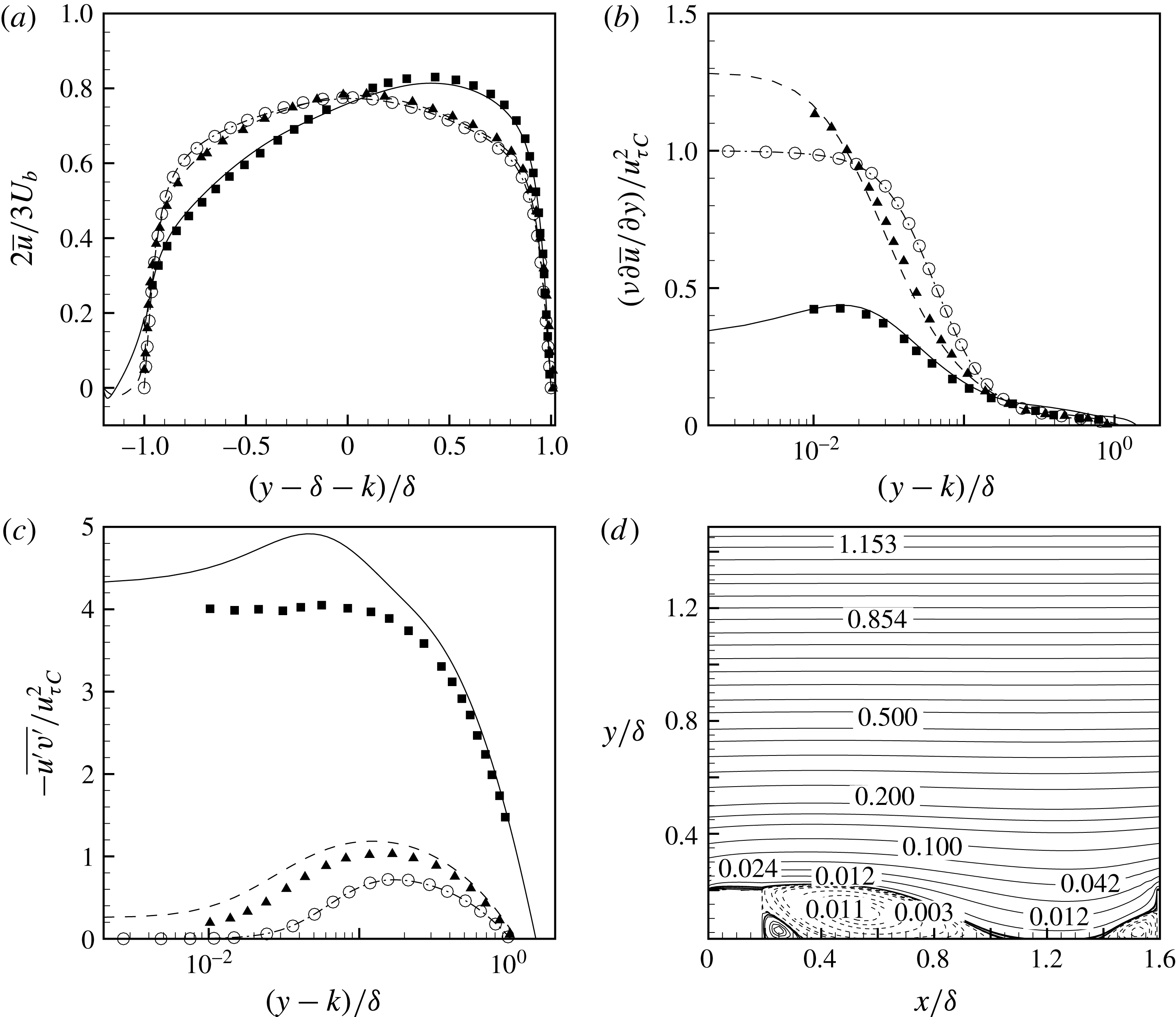
An extensive validation study was carried out to build confidence in the accuracy the simulations. Results from three validation cases are presented in figure 4. One is the low-Reynolds-number, fully developed, smooth-wall channel flow DNS by Moser, Kim & Mansour (Reference Moser, Kim and Mansour1999), at
 $Re_{\unicode[STIX]{x1D70F}}=180$
. The other two have the same
 $Re_{b}$
and a wall-normal domain extent of
 $L_{y}=2\unicode[STIX]{x1D6FF}+k$
, and are taken from Orlandi et al. (Reference Orlandi, Leonardi and Antonia2006). The first of these involves
 $k$
-type roughness with
 $\unicode[STIX]{x1D6FF}/k=5$
and
 $w/k=7$
, while the second has
 $d$
-type roughness with
 $w/k=1$
and the same
 $\unicode[STIX]{x1D6FF}/k$
ratio.
Validation profiles for fully developed channel flows: variation in the wall-normal direction of (a) mean streamwise velocity
 $\overline{u}$
, (b) wall-normal mean-velocity gradient
 $\unicode[STIX]{x1D708}\unicode[STIX]{x2202}\overline{u}/\unicode[STIX]{x2202}y$
, and (c) turbulence shear stress
 $\overline{u^{\prime }v^{\prime }}$
. —— rough-wall flow with
 $w/k=7$
and
 $k/\unicode[STIX]{x1D6FF}=0.2$
, – – – rough-wall flow with
 $w/k=1$
and
 $k/\unicode[STIX]{x1D6FF}=0.2$
, and – ⋅ – ⋅ – smooth-wall channel flow with
 $k/\unicode[STIX]{x1D6FF}=0$
. (d) Mean streamlines for the rough-wall flow with
 $w/k=7$
and
 $k/\unicode[STIX]{x1D6FF}=0.2$
. In these figures
 $u_{\unicode[STIX]{x1D70F}C}$
is the friction velocity at the wall for the smooth-wall channel flow. Filled symbols: data from Orlandi et al. (Reference Orlandi, Leonardi and Antonia2006) and open symbols: data from Moser et al. (Reference Moser, Kim and Mansour1999). Triangles represent
 $d$
-type and squares represent
 $k$
-type roughnesses.

Excellent agreement is obtained with reference data for the smooth-wall channel flow. For the rough walls a very good agreement is achieved by
 $\overline{u}$
and
 $\unicode[STIX]{x1D708}\unicode[STIX]{x2202}\overline{u}/\unicode[STIX]{x2202}y$
as well. However, higher turbulence shear stress
 $\overline{u^{\prime }v^{\prime }}$
values are observed near the top of the roughness elements than were seen by Orlandi et al. (Reference Orlandi, Leonardi and Antonia2006). It is unclear why this difference occurs, but it should be noted that the present simulations have better resolved computational grids, particularly in the wall-normal direction near the bottom wall and near the roughness-element height. The streamlines for the
 $k$
-type roughness case in figure 4(d) demonstrate all the essential mean-flow features observed in Leonardi et al. (Reference Leonardi, Orlandi, Smalley, Djenidi and Antonia2003) and Ikeda & Durbin (Reference Ikeda and Durbin2007). Among them are the primary separation bubble downstream of the roughness element, a small positive recirculation region nestled between the roughness element and the primary separation bubble, a small separation bubble upstream of the roughness element, and another thin separated film above the roughness element with reattachment just before its trailing edge. The reattachment length of the primary separation bubble is
 $4.7k$
–
 $4.8k$
from the trailing edge of the roughness element. The secondary separation bubble starts at approximately
 $-1.5k$
from the leading edge of the roughness element. These compare favourably with the values of
 ${\sim}4.8k$
and
 $-1.5k$
reported by Leonardi et al. (Reference Leonardi, Orlandi, Smalley, Djenidi and Antonia2003). Additionally, another case from Leonardi et al. (Reference Leonardi, Orlandi, Smalley, Djenidi and Antonia2003) with spacing similar to that used in present test cases (
 $w/k=9$
and
 $L_{y}=2\unicode[STIX]{x1D6FF}$
) was simulated. The computed form drag was
 ${\sim}0.0122$
, within
 $3\,\%$
of the value inferred from their figure 9.
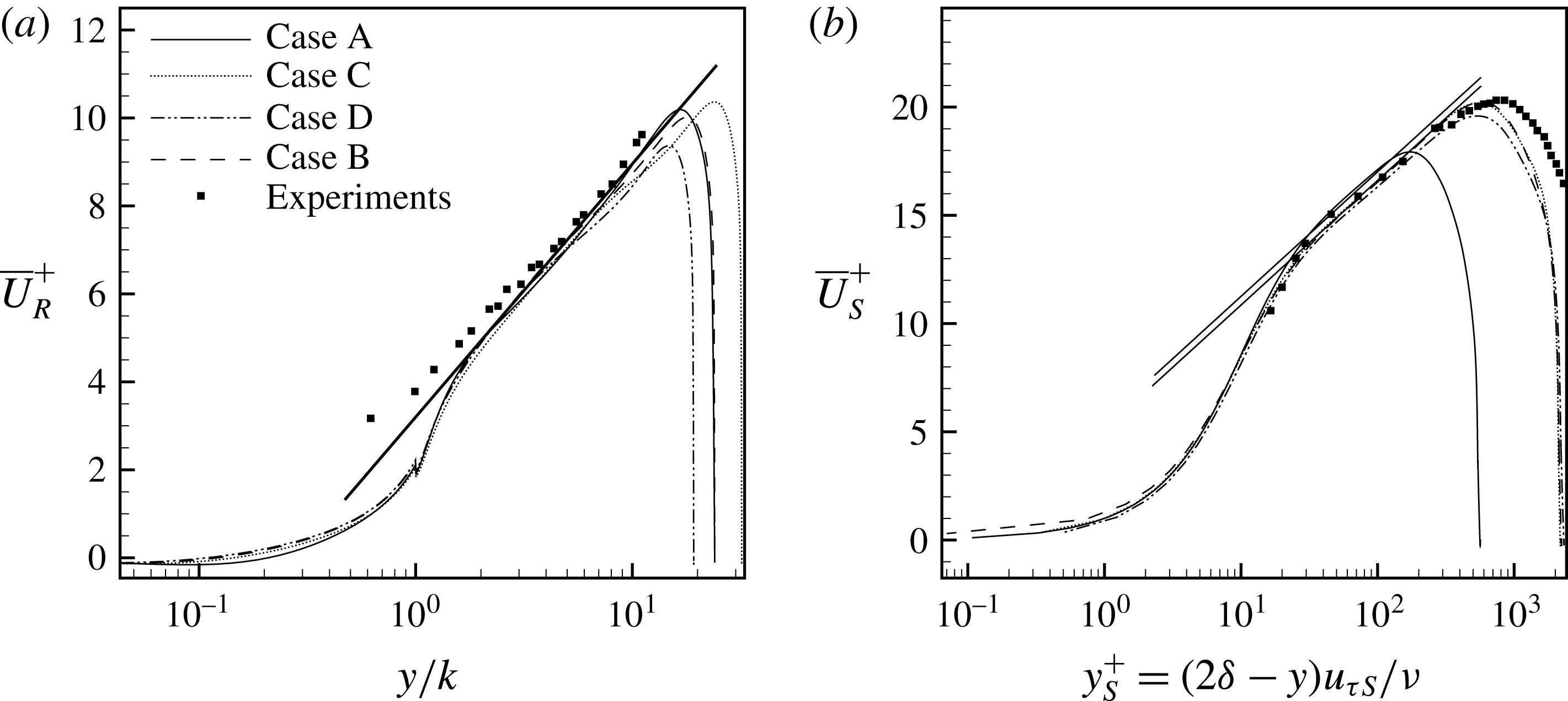
(a) Inner-scaled rough-wall mean streamwise velocity,
 $\overline{U}_{R}^{+}$
, in the fully developed regime. The straight line is given by
 $\overline{U}_{R}^{+}=(1/0.40)\ln (y/k)+3.2$
. (b) Inner-scaled upper smooth-wall mean streamwise velocity,
 $\overline{U}_{S}^{+}$
, in the fully developed regime. The straight lines are given by
 $\overline{U}_{S}^{+}=(1/0.40)\log (y_{s}^{+})+C$
. The additive constant values of
 $C$
are
 $5.1$
and
 $5.5$
. Symbols: experiments by Hanjalic & Launder (Reference Hanjalic and Launder1972).

3.2 Fully developed regime
Figure 5 shows the inner-scaled mean streamwise velocity profiles at both the bottom rough wall and the upper smooth wall, in the fully developed regime. Hot-wire measurements by Hanjalic & Launder (Reference Hanjalic and Launder1972) are also shown. The experimental data were obtained at the same
 $w/k$
as in the present work – albeit one with a comparatively small
 $\unicode[STIX]{x1D6FF}/k=8.5$
. These measurements were taken at a Reynolds number of
 $Re_{U_{max}}=U_{max}\unicode[STIX]{x1D6FF}/\unicode[STIX]{x1D708}=35,500$
, where
 $U_{max}$
is the maximum mean velocity. Above both rough and smooth walls, and within the log-law region, the comparison with the DNS results is favourable. The displacement to the right in figure 5(b) is a result of a higher
 $Re_{\unicode[STIX]{x1D70F}S}$
for the lab experiments, and the small overshoot is more likely due to a smaller
 $\unicode[STIX]{x1D6FF}/k$
ratio. The non-dimensional friction velocity on the bottom rough wall
 $u_{\unicode[STIX]{x1D70F}_{R}}$
is computed from the viscous drag
 $$\begin{eqnarray}\displaystyle & \displaystyle D_{v}=(\unicode[STIX]{x1D708}/U_{b}^{2})(1/L_{fdr})\int _{0}^{L_{fdr}}(\unicode[STIX]{x2202}\overline{U}/\unicode[STIX]{x2202}y)|_{y=y^{h}}\,\text{d}x & \displaystyle\end{eqnarray}$$
on the bottom wall and top of the roughness elements (the height of these two different types of no-slip surfaces is indicated here by
 $y=y^{h}$
) plus the form drag
 $$\begin{eqnarray}\displaystyle & \displaystyle D_{p}=(1/\unicode[STIX]{x1D70C}U_{b}^{2})(1/L_{fdr})\mathop{\sum }_{n=1}^{N}\int _{0}^{k}(\overline{P}_{f}-\overline{P}_{b})\,\text{d}y & \displaystyle\end{eqnarray}$$
due to the pressure difference across these discrete roughness elements:
 $u_{\unicode[STIX]{x1D70F}R}^{2}=D_{p}+D_{v}$
. In the expression for
 $D_{p}$
,
 $N$
is the number of roughness elements in the fully developed regime, and
 $\overline{P}_{f}$
and
 $\overline{P}_{b}$
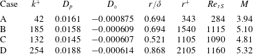
are mean pressure values on the front and back of the roughness elements. Details on the parameters obtained in the fully developed regime are listed in table 4. For test cases A and B the two
 $u_{\unicode[STIX]{x1D70F}R}$
values are within
 $0.6\,\%$
of each other, thus demonstrating their fully rough nature. The contribution of
 $D_{v}$
is only a very small fraction of the entire
 $u_{\unicode[STIX]{x1D70F}R}^{2}$
–
 $5.7\,\%$
for case A,
 $3.9\,\%$
for case B,
 $4.4\,\%$
for case C and
 $3.3\,\%$
for case D. The form-drag contribution,
 $D_{p}$
, is essentially the same for cases A and B, which have the same
 $\unicode[STIX]{x1D6FF}/k$
; whereas
 $D_{v}$
shows an approximately
 $30\,\%$
change for the high-
 $Re_{b}$
simulations. Also, the net contribution of
 $D_{v}$
is negative due to the mean separation bubbles forming behind and in front of the roughness elements.
Parameters obtained in the fully developed regime. Here the roughness Reynolds number
 $k^{+}$
is defined as
 $k^{+}=u_{\unicode[STIX]{x1D70F}R}k/\unicode[STIX]{x1D708}$
.

The effective sand-grain roughness,
 $r$
, is estimated as
 $r=k\exp [-\unicode[STIX]{x1D705}(B-8.5)]$
, where
 $\unicode[STIX]{x1D705}$
is the von Kármán constant and
 $B$
is the wall intercept of the log-law, fitted to the inner-scaled mean streamwise velocity profiles. The value of
 $B=3.2$
is the same as found by Hanjalic & Launder (Reference Hanjalic and Launder1972) and Ikeda & Durbin (Reference Ikeda and Durbin2007). For our test cases
 $r/k=8.33$
, which is comparable to the ratio obtained by Volino et al. (Reference Volino, Schultz and Flack2011) for their boundary-layer lab experiments, involving small square bars. The effective sand-grain roughness is a significant fraction of the channel half-height (
 $r=0.694\unicode[STIX]{x1D6FF}$
); however,
 $r$
is merely a parameter that equates the log-layer displacement with the experiments by Nikuradse (Reference Nikuradse1933). Ikeda & Durbin (Reference Ikeda and Durbin2007) obtained an effective sand-grain roughness length of
 $r=1.09\unicode[STIX]{x1D6FF}$
for their rib-roughened channel flow simulations.
The upper, smooth wall establishes a log-law region with wall intercepts of
 $C=5.5$
and
 $C=5.1$
, as shown in figure 5(b). These are similar to intercepts measured in fully developed smooth-wall channel flows of comparable
 $Re_{b}$
. But the friction velocity at this wall,
 $u_{\unicode[STIX]{x1D70F}S}$
, is higher than equivalent fully developed smooth-wall channel flows, which signals an interaction between the two walls.
Inner-scaled mean streamwise velocity at different streamwise positions in the fully developed rough-wall regime for case B.

 $s/k=1.13$
, – – – at
 $s/k=2.80$
, – ⋅ – ⋅ – at
 $s/k=4.50$
,
 $\cdots \cdots$
at
 $s/k=6.25$
, — ⋅ ⋅ — at
 $s/k=7.80$
and

 $s/k=9.50$
. The straight line is given by:
 $\overline{U}_{R}^{+}=(1/0.40)\ln (y/k)+3.2$
.
 $s$
is the distance from the trailing edge of a roughness element.

We can define a roughness sublayer (RS) that is dynamically influenced by the underlying rough wall, and that is spatially inhomogeneous. For case B, as shown in figure 6, the extent of this RS can be identified as the wall-normal distance from the lower wall where horizontal inhomogeneity in the mean velocity disappears. It is at
 $y/k\approx 4.5$
; for other cases too, this height is between
 $y/k=4$
and 5. Additionally, it is noticeable from figures 5(a) and 6 that the fitted log-law enters the RS, extending down to approximately
 $y\approx 2k$
. Ikeda & Durbin (Reference Ikeda and Durbin2007) used the onset of the fitted log-law for mean velocity and
 $P/\unicode[STIX]{x1D716}\approx 1$
to identify their roughness sublayer height as
 $y\approx 2k$
, where
 $P$
and
 $\unicode[STIX]{x1D716}$
are the production and dissipation rates of the turbulence kinetic energy.
Above smooth-wall boundary layers, Wei et al. (Reference Wei, Fife, Klewicki and McMurtry2005) defined the onset of the log-law region,
 $y_{I}$
, as the wall-normal location where viscous forces lose dominance. Using the mean-momentum budget terms, they showed that
 $y_{I}$
occurred just above the vertical location of the maxima of turbulence shear stress, at
 $y_{m}$
. For rough-wall boundary layers, Mehdi, Klewicki & White (Reference Mehdi, Klewicki and White2013) proposed
 $y_{I}=C_{I}y_{m}$
, with
 $C_{I}\sim O(1)$
. Their argument was based on qualitative similarity of mean dynamics with smooth-wall flows in the zone where transition to the log-law region takes place. They further proposed functions of the following form for estimating
 $y_{m}$
:
 $$\begin{eqnarray}\displaystyle & \displaystyle y_{m}=C_{m}(\unicode[STIX]{x1D708}/u_{\unicode[STIX]{x1D70F}})^{a}r^{b}\unicode[STIX]{x1D6FF}^{c}. & \displaystyle\end{eqnarray}$$
Here,
 $C_{m},a,b$
and
 $c$
are empirically determined constants based on three different classification regimes of
 $y_{m}/r$
. Using their function for
 $y_{m}/r<O(1)$
, for case B,
 $y_{m}\approx 1.18k$
, which is close to the exact location at
 $y_{m}=1.25k$
. Based on this estimate of
 $y_{m}$
and the above-mentioned approximate location for the onset of the log-law region, at
 $y\approx 2k$
,
 $C_{m}\approx 1.70\sim O(1)$
.
Following Andreopoulos & Wood (Reference Andreopoulos and Wood1982) the hydrodynamic roughness length scales can be used to compute the strength of roughness step
 $M=\ln (z_{r}/z_{s})$
in order to quantify the degree of perturbation for these RTS simulations. Here,
 $z_{r}=r\exp (-8.5\unicode[STIX]{x1D705})$
is the hydrodynamic roughness length scale in the fully developed rough-wall regime, and
 $z_{s}=(\unicode[STIX]{x1D708}/u_{\unicode[STIX]{x1D70F}})\exp (-\unicode[STIX]{x1D705}C)$
is an equivalent roughness length scale from a separate fully developed smooth-wall channel flow at the same
 $Re_{b}$
. The expression for
 $z_{s}$
is derived by equating the log-law in terms of the viscous length scale,
 $\unicode[STIX]{x1D6FF}_{\unicode[STIX]{x1D708}}=\unicode[STIX]{x1D708}/u_{\unicode[STIX]{x1D70F}}$
, to an equivalent log-law in terms of a hydrodynamic roughness length scale,
 $z_{s}$
. Values of
 $M$
given in table 4 are comparable to
 $M=3.4$
and
 $5.1$
, reported by Hanson & Ganapathisubramani (Reference Hanson and Ganapathisubramani2016). Taylor et al. (Reference Taylor, Taylor, Hosni and Coleman1993) reported
 $M=3.15$
for their RTS boundary-layer experiments. It should be noted that, for cases A and B, the difference in
 $M$
is due to different downstream length scales,
 $\unicode[STIX]{x1D6FF}_{v}$
, and the difference in
 $M$
between cases B, C and D is due to different upstream length scales,
 $r$
.
3.3 Skin friction
The skin-friction coefficient
 $C_{f}=(\unicode[STIX]{x1D708}/2.25U_{b}^{2})(\unicode[STIX]{x2202}\overline{U}/\unicode[STIX]{x2202}y)$
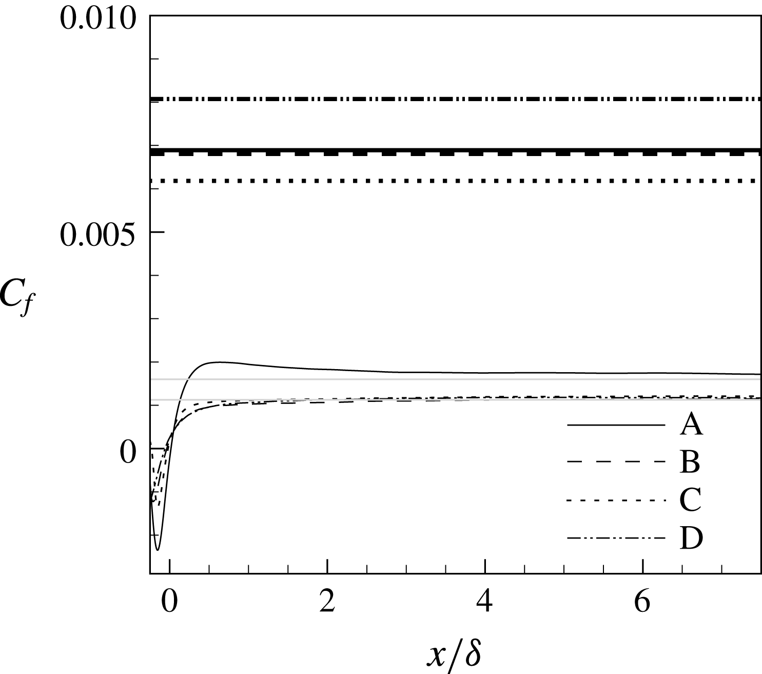
in the developing, smooth-wall regime is plotted in figure 7. It first reduces sharply, to levels well below the fully developed smooth-wall levels (grey lines) before growing quickly and then gradually levelling off (immediately after the step change in roughness, it becomes negative due to the separation bubble following the last roughness element). The skin-friction profiles above the rough wall in figure 7 include contributions from both viscous and form drags. By
 $x\approx 2\unicode[STIX]{x1D6FF}$
, the high-Reynolds-number cases plateau very close to fully developed smooth-wall levels. It would, however, be misleading to conclude that the
 $C_{f}$
has equilibrated. Its incomplete recovery is more evident for the low-Reynolds-number case. Close inspection of
 $(1/\unicode[STIX]{x1D70C})\unicode[STIX]{x2202}\overline{P}/\unicode[STIX]{x2202}x$
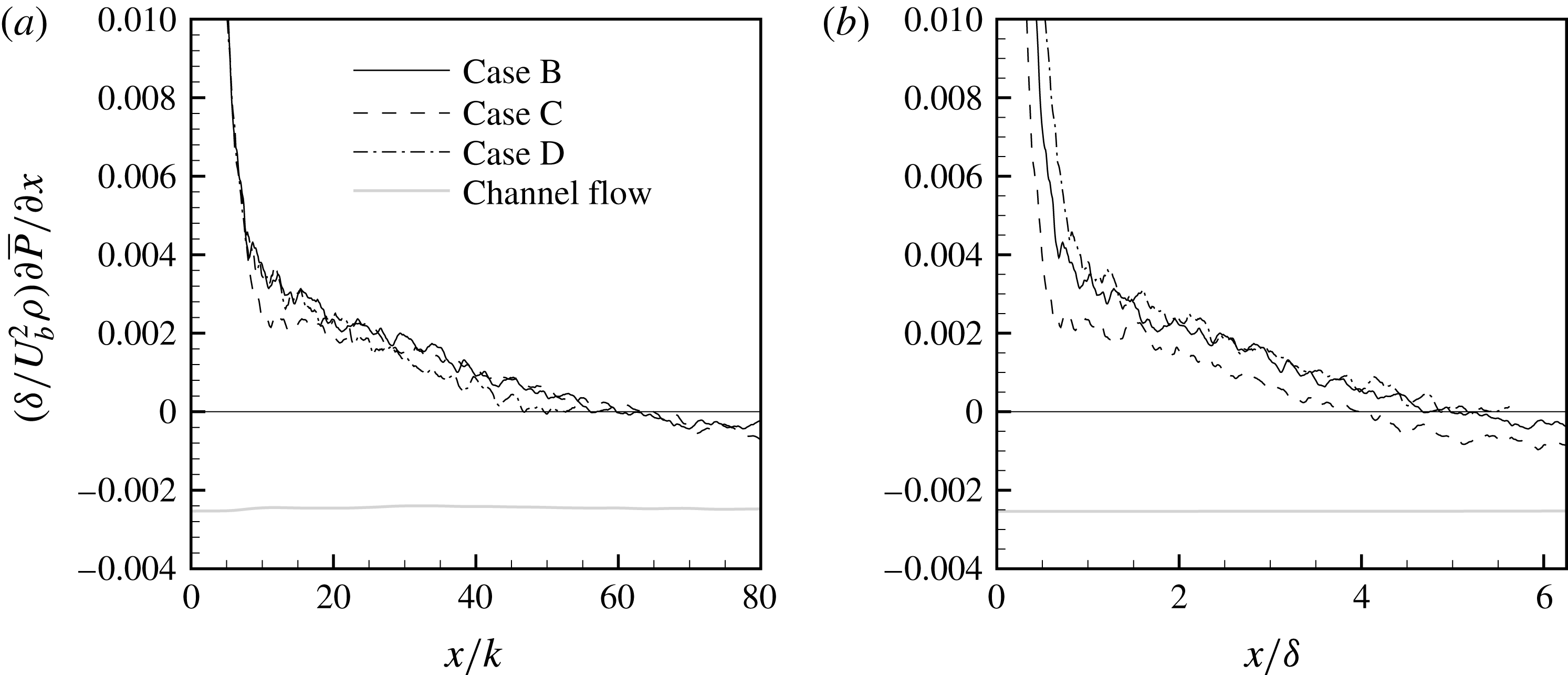
at the wall shows that it is adverse over most of the domain, becoming negative near the end of the domain (figure 8). Preliminary results, not included here, from RTS simulations using cube roughness evidence this same behaviour.
Skin-friction,
 $C_{f}$
, profiles in the developing, smooth-wall regime. Bold black lines: fully developed rough-wall regimes; thin black lines: fully developed smooth-wall channel flows.

Streamwise variation of
 $(1/\unicode[STIX]{x1D70C})\unicode[STIX]{x2202}\overline{P}/\unicode[STIX]{x2202}x$
at the lower wall in the developing regime, with
 $x$
scaled by (a) the roughness length scale,
 $k$
, and (b) the channel half-height,
 $\unicode[STIX]{x1D6FF}$
.

Case A shows a steeper increase of
 $C_{f}$
compared to the other cases, which is consistent with observations made by Antonia & Luxton (Reference Antonia and Luxton1972). The initial recovery of
 $C_{f}$
is different for the three cases at high Reynolds numbers; they do not collapse when the streamwise distance is normalized by either
 $\unicode[STIX]{x1D6FF}$
or
 $k$
. However, the initial response of
 $(1/\unicode[STIX]{x1D70C})\unicode[STIX]{x2202}\overline{P}/\unicode[STIX]{x2202}x$
at the wall does collapse when plotted against
 $x/k$
(figure 8
a), but not when the streamwise distance is scaled by
 $\unicode[STIX]{x1D6FF}$
(figure 8
b). This implies that, for the type of the roughness considered and for initial recovery, the streamwise variation (
 $x/k$
) of the pressure gradient at the wall can be determined independently of
 $\unicode[STIX]{x1D6FF}/k$
.
 $(1/\unicode[STIX]{x1D70C})\unicode[STIX]{x2202}\overline{P}/\unicode[STIX]{x2202}x$
can be extrapolated to large
 $x/k$
, to estimate the streamwise distance required to reach the fully developed, smooth-wall gradient. A nonlinear regression fit, using a dissociation curve (Hill Reference Hill1913), estimates this distance as
 $x\approx 450k$
(or
 $37\unicode[STIX]{x1D6FF}$
).
3.4 Mean velocity
After the step change in roughness the retarded mean flow above the rough wall experiences strong near-wall acceleration, as shown in figure 9 for case A. By conservation of mass-flow rate, this is compensated by deceleration further away from the bottom wall, and both acceleration and deceleration gradually decrease in magnitude with downstream distance. By the last streamwise station in figure 9, at
 $x/\unicode[STIX]{x1D6FF}=7.1$
, the mean velocity has not recovered to the fully developed smooth-wall profile, which is the symmetric grey curve.
Outer-scaled mean streamwise velocity
 $\overline{U}/U_{b}$
in the developing section scaled from the lower wall for case A. —— in the fully developed rough-wall regime, —— at
 $x/\unicode[STIX]{x1D6FF}=0.42$
, – – – at
 $x/\unicode[STIX]{x1D6FF}=2.08$
, – ⋅ – ⋅ – at
 $x/\unicode[STIX]{x1D6FF}=3.75$
,
 $\cdots \cdots$
at
 $x/\unicode[STIX]{x1D6FF}=5.42$
, — ⋅ ⋅ — at
 $x/\unicode[STIX]{x1D6FF}=7.08$
,


Outer-scaled mean streamwise velocity
 $\overline{U}/U_{b}$
at different streamwise stations for the high-Reynolds-number cases. —— case B, – – – case C, – ⋅ – ⋅ – case D and


Mean streamwise velocity for case B in the developing, smooth-wall regime scaled from (a,b) the bottom wall and in inner coordinates,
 $\overline{U}^{+}$
and
 $y^{+}$
; (c) the top wall and in inner coordinates,
 $\overline{U}_{u}^{+}$
and
 $y_{u}^{+}$
. (a,c) —— in the fully developed rough-wall regime, —— at
 $x/\unicode[STIX]{x1D6FF}=0.42$
, – – – at
 $x/\unicode[STIX]{x1D6FF}=2.08$
, – ⋅ – ⋅ – at
 $x/\unicode[STIX]{x1D6FF}=3.75$
,
 $\cdots \cdots$
at
 $x/\unicode[STIX]{x1D6FF}=5.42$
, — ⋅ ⋅ — at
 $x/\unicode[STIX]{x1D6FF}=7.08$
,

 $x/\unicode[STIX]{x1D6FF}=0.08$
, – – – at
 $x/\unicode[STIX]{x1D6FF}=0.17$
, – ⋅ – ⋅ – at
 $x/\unicode[STIX]{x1D6FF}=0.25$
,
 $\cdots \cdots$
at
 $x/\unicode[STIX]{x1D6FF}=0.33$
, — ⋅ ⋅ — at
 $x/\unicode[STIX]{x1D6FF}=0.42$
,


The point of intersection between two successive and equally spaced streamwise stations from figure 9 has been used as an indicator of the ‘internal layer’ height (Antonia & Luxton Reference Antonia and Luxton1972). It moves away from the wall with downstream distance. However, the consequent mean-flow deceleration above these points of intersection is evidence that, for such internal flows, the entire wall-normal domain is affected by the change in roughness, and the idea of an internal boundary layer is not pertinent. Figure 10 shows the mean-velocity profiles in the developing smooth-wall regime for the three high-Reynolds-number cases. The profiles in outer variables are very similar. A hyperbolic-decline curve was fitted to the downstream decay of the outer peak of
 $\overline{U}$
. For case B, it estimates the streamwise distance needed to reduce to near-fully-developed, smooth-wall channel flow levels at
 $x=55\unicode[STIX]{x1D6FF}$
.
The inner-scaled mean velocity
 $\overline{U}^{+}$
in the developing smooth-wall regime is shown in figure 11(a) for case B. Like the outer-scaled velocity profiles, it too shows quick initial recovery, but a fully developed, smooth-wall profile has not developed by the domain exit. In the fully developed rough-wall regime, mean-velocity levels are well below and towards the right of the developing regime profiles, due to the higher to high friction velocity
 $u_{\unicode[STIX]{x1D70F}R}$
. Very close to the bottom wall (
 $y^{+}\leqslant 20$
) nearly complete recovery and good collapse of the profiles with smooth-wall channel flow occurs by the end of the domain.
By the second streamwise station, at
 $x=2.08$
in figure 11(a),
 $\overline{U}^{+}$
has attained a qualitative shape that remains essentially unchanged and gradually shifts upwards with downstream distance. This slow upward shift is contrary to the trend observed by Hanson & Ganapathisubramani (Reference Hanson and Ganapathisubramani2016). With downstream fetch, their profiles were initially pushed up, well above the smooth-wall level (a consequence of low
 $u_{\unicode[STIX]{x1D70F}}$
) and then settled down towards it. The mean velocity results in our initial strong non-equilibrium zone, between
 $0<x/\unicode[STIX]{x1D6FF}<0.5$
, are plotted in figure 11(b), and demonstrate this decay trend – but only at short distances where
 $C_{f}$
is increasing.
Using these inner-scaled plots, it might seem interesting to investigate the existence of a log-law region in the transitional regime and possibly to fit log-law profiles. Marusic et al. (Reference Marusic, Monty, Hultmark and Smits2013), for high Reynolds number, fully developed, smooth-wall boundary layers, provided empirical functions for the bounds of the log-law region:
 $y_{I}^{+}=3\sqrt{Re_{\unicode[STIX]{x1D70F}}}$
for lower onset location and
 $y^{+}=0.15Re_{\unicode[STIX]{x1D70F}}$
for the upper bound, which for the current
 $Re_{\unicode[STIX]{x1D70F}}$
falls between
 $90\sim 140$
. After the first streamwise station in figure 11(a), at the wall-normal height where a log-law might possibly exist, it might appear that
 $\unicode[STIX]{x1D705}$
is higher than typical levels of
 $0.40$
–
 $0.41$
. This is not a warranted conclusion; the impression of a modified
 $\unicode[STIX]{x1D705}$
above
 $y^{+}>40$
–
 $50$
in figure 11(a) is misleading. The large velocity deficit created by roughness persists with downstream distance. The warranted conclusion is that an equilibrium log-law has not established, even by the end of the computational domain.
By contrast, the upper, smooth wall remains near to equilibrium, as evidenced by negligible difference between the profiles at successive streamwise stations and by establishment of the conventional log-law profiles in figure 11(c). The frictional Reynolds number at this wall
 $Re_{\unicode[STIX]{x1D70F}u}=u_{\unicode[STIX]{x1D70F}U}\unicode[STIX]{x1D6FF}/\unicode[STIX]{x1D708}$
for case B shows less than
 $8\,\%$
reduction, from
 $1115$
down to approximately
 $1030$
, between the fully rough region and the last streamwise station. At the last measuring station in the developing regime the top wall shows an
 $Re_{\unicode[STIX]{x1D70F}}$
that is more than
 $10\,\%$
higher than the fully developed smooth-wall channel flow, while on the more active, bottom wall,
 $u_{\unicode[STIX]{x1D70F}}$
has already plateaued very close to the fully developed magnitude. Although inner-scaled profiles are only presented for case B, the trends noted and conclusions drawn also apply to the other cases.
3.5 Turbulence stresses
Profiles of turbulence kinetic energy,
 $K$
, and turbulence stresses in the developing smooth-wall regime are presented in figures 12 and 13. Plots in the fully developed regime exhibit a small discontinuity at
 $y/k=1$
. This is a result of the length of the streamwise averaging changing abruptly at the crests of the roughness elements. The wall-normal location of the outer peaks of
 $\overline{u^{\prime }u^{\prime }}$
in the fully developed rough-wall regime stays virtually fixed at
 $y/\unicode[STIX]{x1D6FF}\approx 0.11,0.11,0.084$
and
 $0.13$
for cases A, B, C and D, respectively, which lies between
 $y/k=1.25$
and 1.35. This is within the
 $y/\unicode[STIX]{x1D6FF}=0.05$
–
 $0.2$
range observed for rough-wall boundary layers (Jimnez Reference Jimnez2004; Jacobi & Mckeon Reference Jacobi and Mckeon2011). Using inner coordinates, the outer peak for case B in the fully developed rough-wall regime is located at approximately
 $y^{+}=600$
. The aforementioned range of
 $y/k=1.25$
–
 $1.35$
also applies to the wall-normal location of the rough-wall peaks of
 $\overline{u^{\prime }v^{\prime }}$
for all four cases.
Normal turbulence stresses and TKE in the developing smooth-wall regime for case B. —— in the fully developed rough-wall regime, —— at
 $x/\unicode[STIX]{x1D6FF}=0.42$
, – – – at
 $x/\unicode[STIX]{x1D6FF}=2.08$
, – ⋅ – ⋅ – at
 $x/\unicode[STIX]{x1D6FF}=3.75$
,
 $\cdots \cdots$
at
 $x/\unicode[STIX]{x1D6FF}=5.42$
, — ⋅ ⋅ — at
 $x/\unicode[STIX]{x1D6FF}=7.08$
,

 $y^{+}=17$
in (b) and
 $y^{+}=14$
in (d).

Turbulence shear stress in the developing smooth-wall regime for case B. —— in the fully developed rough-wall regime, —— at
 $x/\unicode[STIX]{x1D6FF}=0.42$
, – – – at
 $x/\unicode[STIX]{x1D6FF}=2.08$
, – ⋅ – ⋅ – at
 $x/\unicode[STIX]{x1D6FF}=3.75$
,
 $\cdots \cdots$
at
 $x/\unicode[STIX]{x1D6FF}=5.42$
, — ⋅ ⋅ — at
 $x/\unicode[STIX]{x1D6FF}=7.08$
,


From all the plots, particularly those using outer scaling, over the developing smooth wall, higher levels of turbulence, characteristic of the upstream rough wall, persist to the domain exit. Outer peaks, attributable to the rough wall, decay in magnitude with downstream distance, while being driven away from the lower wall. By the last streamwise station, these peaks are still vaguely discernible. However, despite this strong initial decrease and vertical transport, a very large mismatch remains with the fully developed smooth-wall profiles, shown by the light-grey curves in the figures.
By the second streamwise station in figure 12(d), at
 $x/\unicode[STIX]{x1D6FF}\geqslant 2.08$
, the wall-normal gradient of
 $\overline{u^{\prime }u^{\prime }}^{+}$
changes sign from positive to negative in the vicinity of
 $y/\unicode[STIX]{x1D6FF}\approx 0.02$
, indicating the establishment of a near-wall, inner peak. This inner peak is consistent with the near-wall of turbulent flow over smooth walls. Its wall-normal location shows negligible change with downstream distance. By the last streamwise station in figure 12(d), the inner-peak magnitude is still approximately
 $10\,\%$
higher than the fully developed, smooth-wall level. Comments and observation made for the streamwise turbulence stress also apply to the turbulence kinetic energy (TKE), as is evident from figure 12(a,b).
It is worthwhile contrasting the near-wall recovery of the streamwise turbulence stress with that of the outer flow. The near-wall region shows a strong initial recovery, with the profile shape closely matching that of the fully developed smooth wall, after which there is only weak downstream reduction in magnitude. The outer flow, on the other hand, shows a stronger decay rate throughout the horizontal extent of the domain. It remains well above the asymptotic smooth-wall profiles, which have a low level of turbulence in this region.
The turbulence wall normal,
 $\overline{v^{\prime }v^{\prime }}$
, and shear stress,
 $\overline{u^{\prime }v^{\prime }}$
(figures 12
e,f, 13
a,b) present another interesting picture, with the fully developed smooth-wall counterpart having inner-layer peaks that lie further away from the wall. For our low-Reynolds-number case the peak of
 $\overline{v^{\prime }v^{\prime }}$
lies at
 $y^{+}\approx 58$
and of
 $\overline{u^{\prime }v^{\prime }}$
at
 $y^{+}\approx 34$
, while for the high-Reynolds-number case the two are located at
 $y^{+}\approx 105$
and
 $y^{+}\approx 53$
, respectively. At
 $Re_{\unicode[STIX]{x1D70F}}=590$
, Moser et al. (Reference Moser, Kim and Mansour1999) obtained peaks of
 $\overline{v^{\prime }v^{\prime }}^{+}$
at
 $y^{+}\approx 78$
and of
 $\overline{u^{\prime }v^{\prime }}^{+}$
at
 $y^{+}\approx 44$
. Since these peaks for wall-normal and spanwise turbulence stresses are further away from the wall than for
 $\overline{u^{\prime }u^{\prime }}$
, their re-establishment is overshadowed by the higher turbulence magnitudes in the outer flow. This is especially true for
 $\overline{v^{\prime }v^{\prime }}$
, where the near-wall peak is not established at all by the last streamwise station. The near-wall peak for
 $\overline{u^{\prime }v^{\prime }}$
, however, appears to have formed by the second streamwise station, figure 13(b), but it too is obscured by higher, outer-flow turbulence levels. As for the mean-velocity data, discussed earlier, the upper wall shows negligible downstream development, remaining similar to what is seen above the rough wall.
In the near-wall region for fully developed smooth-wall flows,
 $$\begin{eqnarray}\displaystyle & \displaystyle \overline{u^{\prime }u^{\prime }}>\overline{w^{\prime }w^{\prime }}>\overline{v^{\prime }v^{\prime }}, & \displaystyle\end{eqnarray}$$
whereas for fully developed rib-roughened rough-wall flows
 $$\begin{eqnarray}\displaystyle & \displaystyle \overline{w^{\prime }w^{\prime }}>\overline{u^{\prime }u^{\prime }}>\overline{v^{\prime }v^{\prime }}. & \displaystyle\end{eqnarray}$$
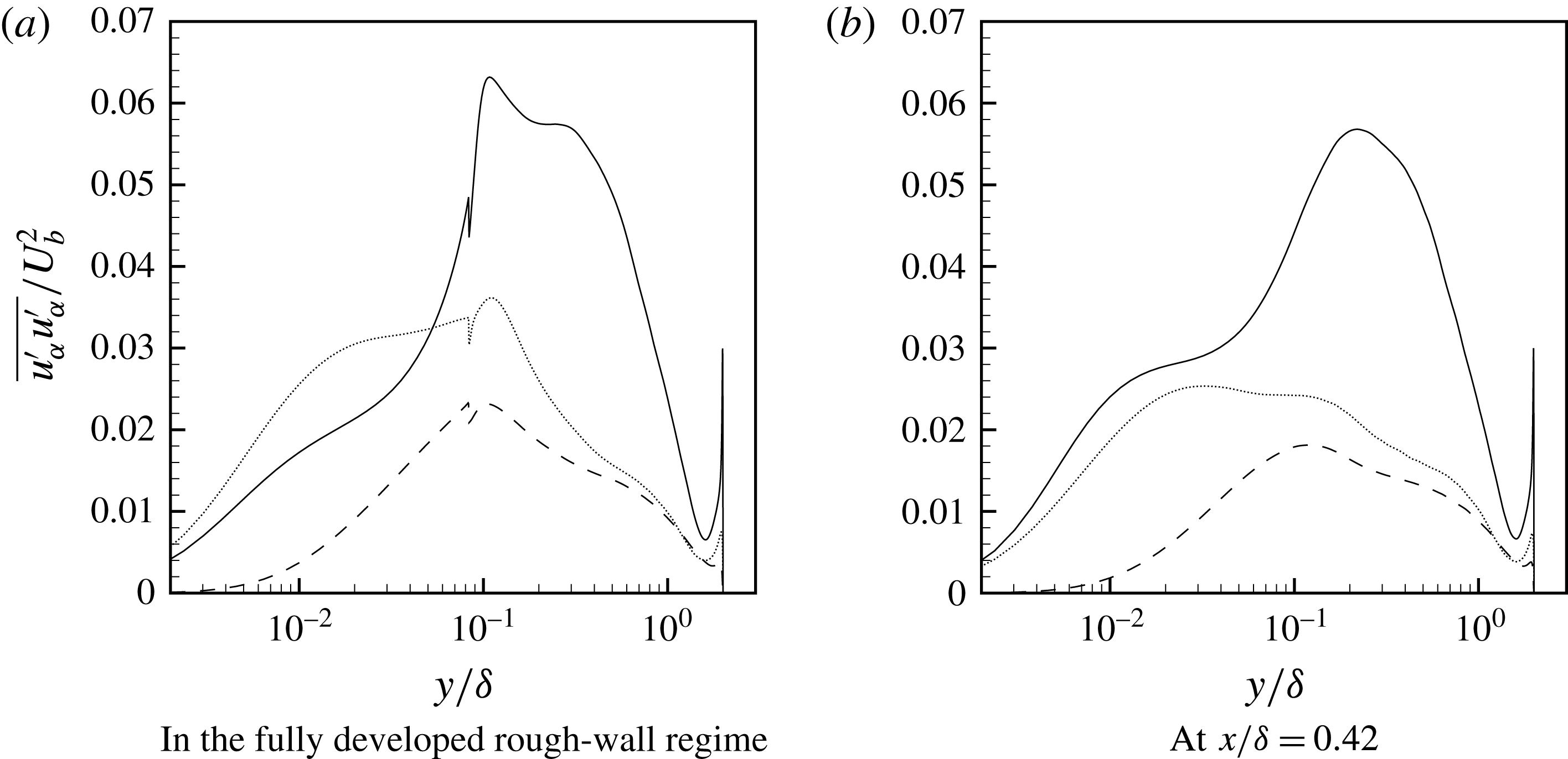
Ikeda & Durbin (Reference Ikeda and Durbin2007), who reported this particular precedence of turbulence stresses for rough-wall flows, also noted that the two-dimensional, square ribs suppress the streamwise stress, which in turn enhances the spanwise motions. In our transitional regime, however, at the first streamwise station located downstream of the step change (
 $x/\unicode[STIX]{x1D6FF}=0.42$
) the effect of upstream roughness elements on the near-wall turbulence anisotropy has already been lost and the normal stresses have reattained their smooth-wall hierarchy:
 $\overline{u^{\prime }u^{\prime }}>\overline{w^{\prime }w^{\prime }}$
(see figure 14). This is understandable because, once the roughness elements are removed, the source for damping of streamwise turbulence motions disappears, allowing them to increase above the spanwise motions.
Normal turbulence stresses at fixed streamwise locations for case B. ——
 $\overline{u^{\prime }u^{\prime }}/U_{b}^{2}$
, – – –
 $\overline{v^{\prime }v^{\prime }}/U_{b}^{2}$
and
 $\cdots \cdots$
 $\overline{w^{\prime }w^{\prime }}/U_{b}^{2}$
.

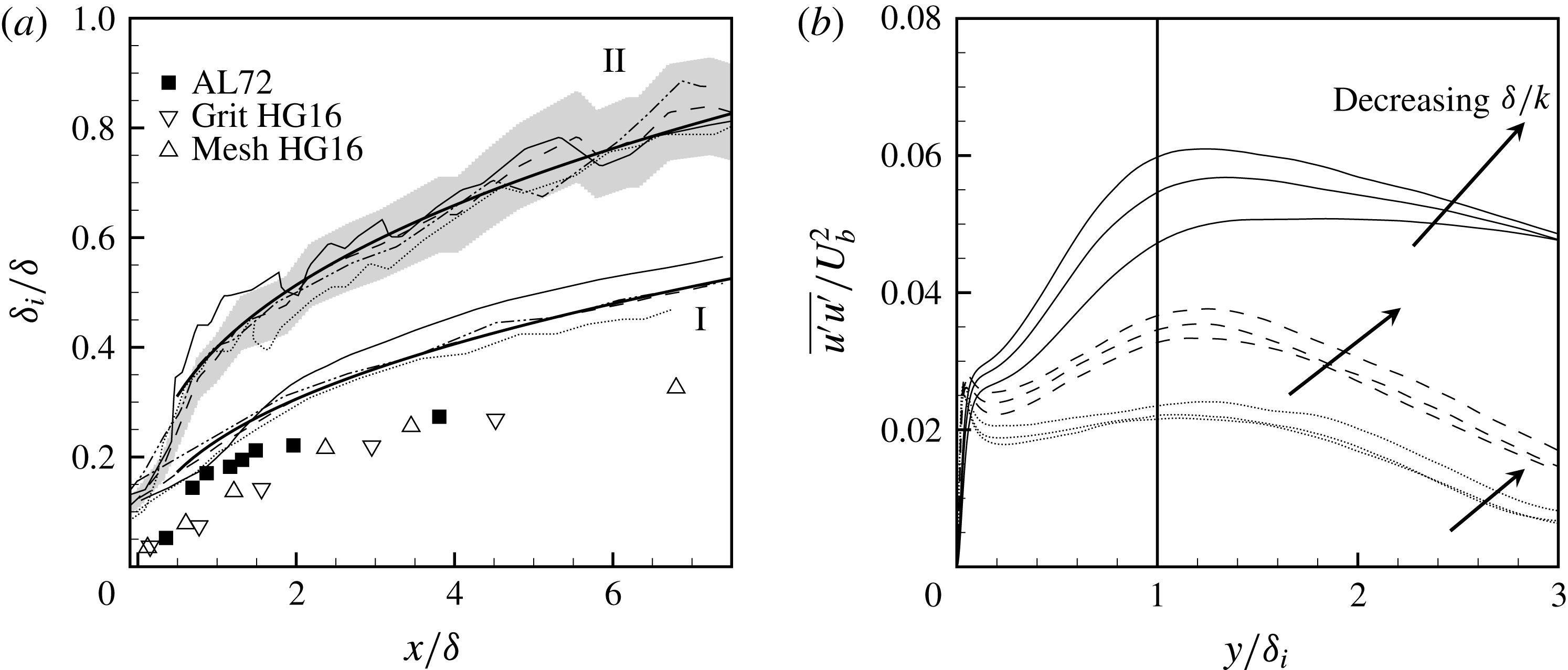
(a) IBL thickness profiles for RTS test cases; symbols: from lab experiments by Antonia & Luxton (Reference Antonia and Luxton1972) and Hanson & Ganapathisubramani (Reference Hanson and Ganapathisubramani2016).
—— represents the fitted power laws:
 $\unicode[STIX]{x1D6FF}_{i}/\unicode[STIX]{x1D6FF}\sim (x/\unicode[STIX]{x1D6FF})^{0.41}$
for the set of profiles labelled I and
 $\unicode[STIX]{x1D6FF}_{i}/\unicode[STIX]{x1D6FF}\sim (x/\unicode[STIX]{x1D6FF})^{0.36}$
for the set of profiles labelled II. The grey envelope indicates the
 $\pm 10\,\%$
extent for case B. —— case B, – – – case C and
 $\cdots \cdots$
case D. (b) Profiles of
 $\overline{u^{\prime }u^{\prime }}$
in the developing regime as a function of
 $y/\unicode[STIX]{x1D6FF}_{i}$
. —— at
 $x/\unicode[STIX]{x1D6FF}=0.42$
, – – – at
 $x/\unicode[STIX]{x1D6FF}=3.75$
,
 $\cdots \cdots$
at
 $x/\unicode[STIX]{x1D6FF}=7.08$
,
—— at
 $y/\unicode[STIX]{x1D6FF}_{i}=1.00$
.

(a) Downstream variation of the outer peaks of
 $\overline{u^{\prime }u^{\prime }}$
and
 $\overline{u^{\prime }v^{\prime }}$
as a function of
 $x/k$
. (b) Downstream growth of the wall-normal location,
 $y/k$
, of
 $\overline{u^{\prime }u^{\prime }}$
and
 $\overline{u^{\prime }v^{\prime }}$
with
 $x/k$
.
 $\cdots \cdots$
for both (a) and (b) represents profiles of approximate fitted functions.

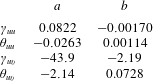
Values of the unknowns in the interpolation functions for
 $\unicode[STIX]{x1D6FE}=a+b(\unicode[STIX]{x1D6FF}/k)$
and
 $\unicode[STIX]{x1D703}=a+b(\unicode[STIX]{x1D6FF}/k)$
.

Although the role of the internal boundary-layer (IBL) height,
 $\unicode[STIX]{x1D6FF}_{i}$
, might not be apparent, its growth rate and utility as a length scale for normalizing the wall-normal coordinate could prove instructive. Figure 15(a) shows the downstream variation of the IBL heights, which are defined as the wall-normal location where the developing, smooth-wall velocity first crosses the upstream, rough-wall mean-velocity profile. The fitted power law
 $\unicode[STIX]{x1D6FF}_{i}\propto x^{0.41}$
agrees well with the trend of
 $\unicode[STIX]{x1D6FF}_{i}\propto x^{0.43}$
reported by Antonia & Luxton (Reference Antonia and Luxton1972). Additionally, IBL profiles estimated by identifying the wall-normal location where
 $\unicode[STIX]{x2202}\overline{U}/\unicode[STIX]{x2202}x$
vanishes (Antonia & Luxton Reference Antonia and Luxton1972) are also shown in 15(a) and labelled II. The lack of smoothness in these IBL profiles is due to difficulty in discerning a precise location for
 $\unicode[STIX]{x2202}\overline{U}/\unicode[STIX]{x2202}x=0$
. Nonetheless, there does not appear to be a systematic difference in the growth rate for different test cases, and a major fraction of the profiles lie within the
 $\pm 10\,\%$
envelope of case B. Compared to the experimental results in figure 15(a), the present
 $\unicode[STIX]{x1D6FF}_{i}$
are much larger. For channel flows, due to continuity, the entire wall-normal domain is affected by the step change in roughness. This is shown by mean-flow acceleration near the lower wall and mean deceleration further away from it in figure 9.
Downstream development of
 $\overline{u^{\prime }u^{\prime }}$
as a function of
 $y/\unicode[STIX]{x1D6FF}_{i}$
is reported in figure 15(b). Here, we use the first definition of IBL. No collapse of profiles is observed within the streamwise extent examined. The same was seen for other turbulence stresses. One concludes from the lack of collapse that
 $\unicode[STIX]{x1D6FF}_{i}$
is not a similarity length scale. Furthermore, it is misleading to construe
 $\unicode[STIX]{x1D6FF}_{i}$
as a demarcator of a developing mean-flow region below an unaffected, upstream region. Rather, it should simply be regarded as a point where the developing mean velocity equals the velocity above the rough wall.
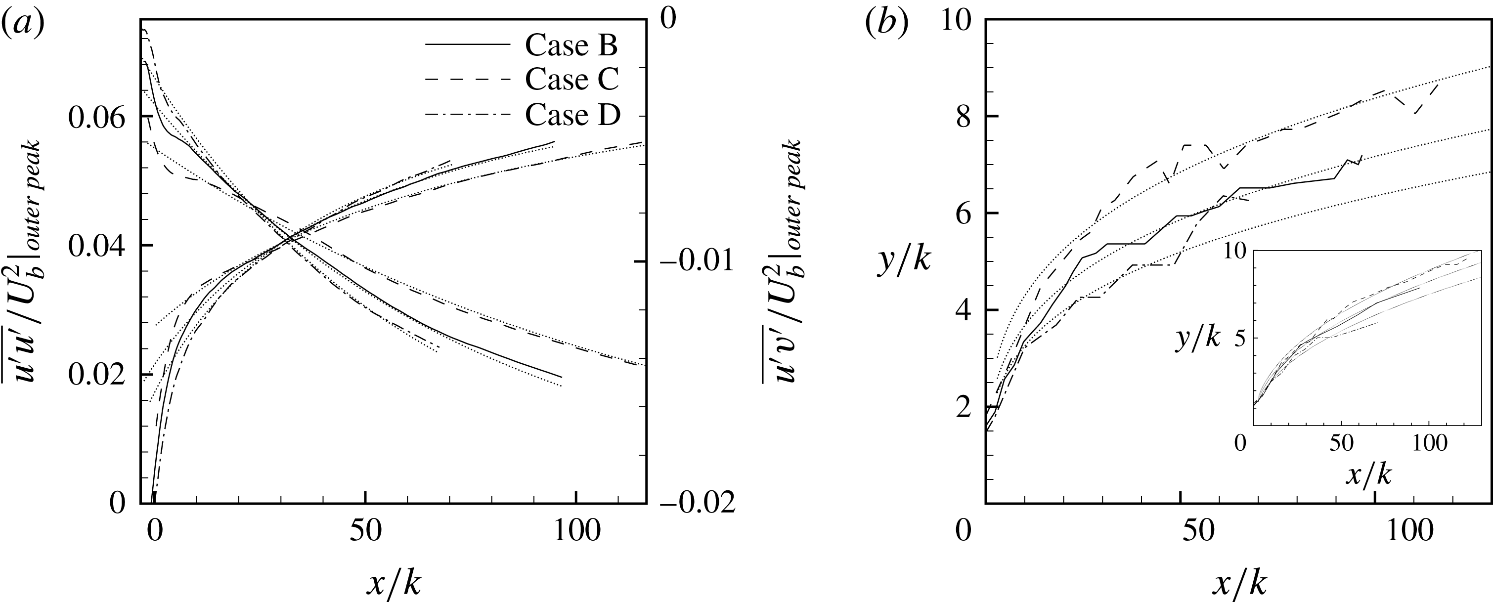
The behaviour of the outer peaks of the Reynolds stresses can be used to estimate the streamwise distance needed by the turbulence stresses to recover to near-fully-developed smooth-wall levels. Figure 16(a) shows the downstream decay of the outer peaks of
 $\overline{u^{\prime }u^{\prime }}$
and
 $\overline{u^{\prime }v^{\prime }}$
. The decay with
 $x/k$
is more severe when
 $\unicode[STIX]{x1D6FF}/k$
is smaller. Approximate curve fits, for
 $x>10k$
, of the type
 $$\begin{eqnarray}\displaystyle & \displaystyle \frac{\overline{u^{\prime }u^{\prime }}}{U_{b}^{2}}|_{outer\,peak}=\unicode[STIX]{x1D6FE}_{uu}\text{e}^{\unicode[STIX]{x1D703}_{uu}(x/k)} & \displaystyle\end{eqnarray}$$
for
 $\overline{u^{\prime }u^{\prime }}$
and
 $$\begin{eqnarray}\displaystyle & \displaystyle \frac{\overline{u^{\prime }v^{\prime }}}{U_{b}^{2}}|_{outer\,peak}=\frac{1}{\unicode[STIX]{x1D6FE}_{uv}+\unicode[STIX]{x1D703}_{uu}(x/k)} & \displaystyle\end{eqnarray}$$
for
 $\overline{u^{\prime }v^{\prime }}$
have been added to the figure. The unknowns
 $\unicode[STIX]{x1D6FE}$
and
 $\unicode[STIX]{x1D703}$
for these three high-Reynolds-number cases are fitted to the form,
 $a+b(\unicode[STIX]{x1D6FF}/k)$
, and the values of
 $a$
and
 $b$
are listed in table 5. The downstream development of the wall-normal location,
 $y/k$
, of these outer peaks of
 $\overline{u^{\prime }u^{\prime }}$
is shown in figure 16(b), while that of
 $\overline{u^{\prime }v^{\prime }}$
is in the inset. Power law fits,
 $(y/k)\sim (x/k)^{m}$
, have also been included in figure 16(b); where
 $m=0.29$
for
 $\overline{u^{\prime }u^{\prime }}$
and
 $m=0.47$
for
 $\overline{u^{\prime }v^{\prime }}$
. Using these approximate functions, we can estimate that the outer peak of
 $\overline{u^{\prime }u^{\prime }}$
for case B would require approximately
 $250k$
(or
 $20.8\unicode[STIX]{x1D6FF}$
) of downstream distance to reach levels similar to those of fully developed smooth-wall channel flows. Rewriting the expression for the outer peaks of
 $\overline{u^{\prime }u^{\prime }}$
as a function of
 $x/\unicode[STIX]{x1D6FF}$
, instead of
 $x/k$
, still results in the exponents displaying a decay rate inversely related to
 $\unicode[STIX]{x1D6FF}/k$
, albeit one that is comparatively slower. This confirms the argument made earlier that the downstream response of the outer-flow turbulence is directly influenced by the roughness size. It is worth mentioning that this downstream distance for recovery to near-fully-developed levels do not imply reversion to complete equilibrium. Even at these distances, the profile of
 $\overline{u^{\prime }u^{\prime }}$
might not necessarily fully match the smooth-wall equivalents.
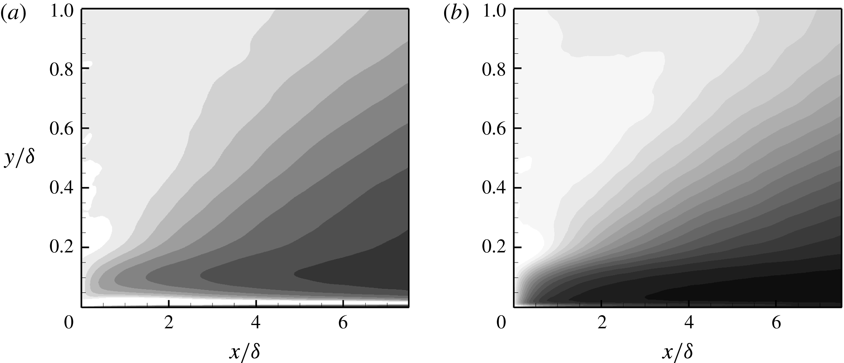
Normalized recovery magnitudes of turbulence stresses for case B. (
 $a$
)
 $\unicode[STIX]{x1D6FD}_{11}$
, (
 $b$
)
 $\unicode[STIX]{x1D6FD}_{12}$
. Scale: black 0.0, white 1.0.

Let subscript
 $R$
denote values at the start of the smooth-wall regime, and
 $S$
denote fully developed, smooth-wall values. Then
 $$\begin{eqnarray}\displaystyle & \displaystyle \unicode[STIX]{x1D6FD}_{ij}=(\overline{u_{i}^{\prime }u^{\prime }}_{j}-\overline{u_{i}^{\prime }u_{j}^{\prime }}_{S})/(\overline{u_{i}^{\prime }u_{j}^{\prime }}_{R}-\overline{u_{i}^{\prime }u_{j}^{\prime }}_{S}) & \displaystyle\end{eqnarray}$$
(Jacobi & Mckeon Reference Jacobi and Mckeon2011) measures the extent of recovery.
 $\unicode[STIX]{x1D6FD}_{11}$
and
 $\unicode[STIX]{x1D6FD}_{12}$
are contour plotted in figure 17. Darker contours are lower values of
 $\unicode[STIX]{x1D6FD}$
, tending to black at the fully developed, smooth-wall value of
 $\unicode[STIX]{x1D6FD}=0$
.
The presence of a large black patch for
 $\overline{u^{\prime }v^{\prime }}$
close to the wall (
 $y/\unicode[STIX]{x1D6FF}<0.2$
), but above
 $y^{+}=40{-}50$
, indicates its swift recovery.
 $\overline{u^{\prime }u^{\prime }}$
recovers more slowly. This, along with the results of energy spectra presented later in figure 21, supports the argument that large, inactive structures associated with
 $\overline{u^{\prime }u^{\prime }}$
show a relative slow return to their fully developed smooth-wall characteristics. This is in contrast to the near-wall, shear-stress producing motions responsible for
 $\overline{u^{\prime }v^{\prime }}$
. The light-grey regions above approximately
 $y/\unicode[STIX]{x1D6FF}=0.2$
indicate the large deficit, high turbulence outer-flow zone, as seen previously in figures 12 and 13.
Quadrant analysis profiles of
 $\overline{u^{\prime }v^{\prime }}$
for case B. —— in the fully developed rough-wall regime, —— at
 $x/\unicode[STIX]{x1D6FF}=0.42$
, – – – at
 $x/\unicode[STIX]{x1D6FF}=2.08$
, – ⋅ – ⋅ – at
 $x/\unicode[STIX]{x1D6FF}=3.75$
,
 $\cdots \cdots$
at
 $x/\unicode[STIX]{x1D6FF}=5.42$
, — ⋅ ⋅ — at
 $x/\unicode[STIX]{x1D6FF}=7.08$
,


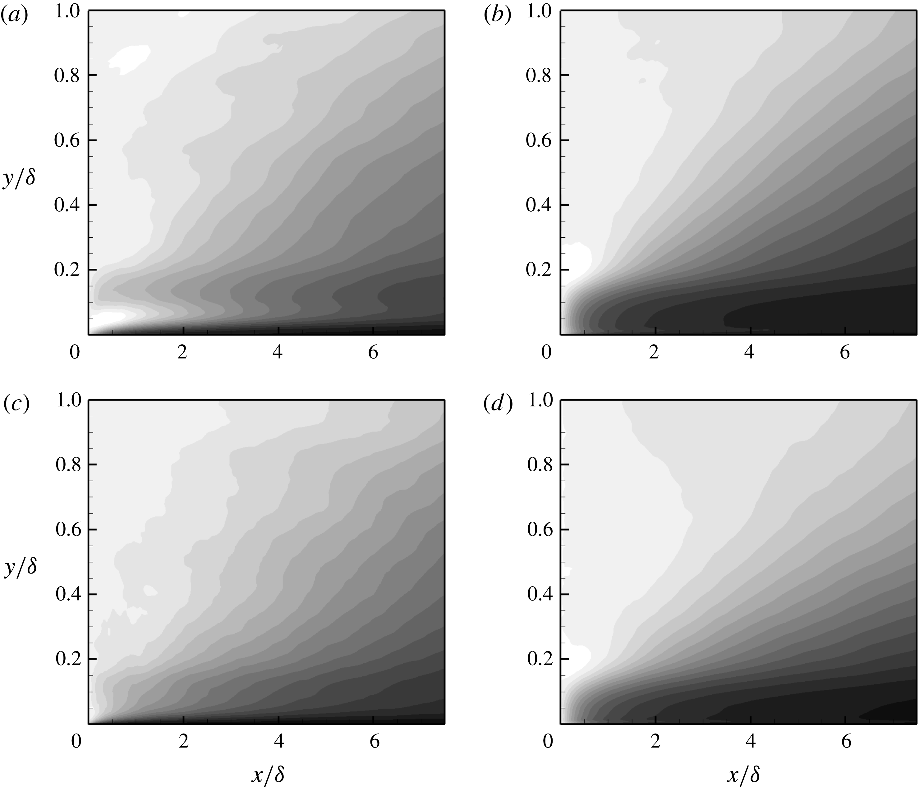
Normalized recovery magnitudes for different components of the quadrant analysis of
 $\overline{u^{\prime }v^{\prime }}$
for case B. (
 $a$
)
 $\unicode[STIX]{x1D6FD}_{Q1}$
, (
 $b$
)
 $\unicode[STIX]{x1D6FD}_{Q2}$
, (
 $c$
)
 $\unicode[STIX]{x1D6FD}_{Q3}$
, (
 $d$
)
 $\unicode[STIX]{x1D6FD}_{Q4}$
. Scale: black 0.0, white 1.0.

To further illustrate the comparatively quick near-wall recovery of shear producing motions, quadrant analysis (Wallace, Eckelmann & Brodkey Reference Wallace, Eckelmann and Brodkey1972; Wallace Reference Wallace2016) is used to identify different components of
 $u^{\prime }v^{\prime }$
that make up the averaged turbulent shear stress
 $\overline{u^{\prime }v^{\prime }}$
. Events from all four quadrants in figure 18 show increased magnitude in the fully developed rough-wall regime. Quadrant 2 (Q2) and quadrant 4 (Q4) events account for negative
 $\overline{u^{\prime }v^{\prime }}$
and, hence, positive production of TKE
 $(P=-\overline{u_{i}^{\prime }u_{j}^{\prime }}\unicode[STIX]{x2202}\overline{u}_{i}/\unicode[STIX]{x2202}x_{j})$
. They are, at least in absolute terms, the dominant events in all three regimes: fully developed rough wall, transitional, and fully developed smooth wall. Results for fully developed smooth walls are well documented in the literature (see Wallace Reference Wallace2016). In the transitional regime, by the last station, Q2 has recovered the most, followed closely by Q4, which is distinctly apparent from the normalized recovery contours given figure 19.
Coherent, instantaneous streamwise motions of alternating high and low momentum are characterized by a large positive and negative
 $u^{\prime }$
, while
 $v^{\prime }$
is smaller, often times by an order of magnitude. Occasionally, however, the low-speed streaks are slowly lifted up, followed by a strong vertical transport away from the wall. This sequence of events was referred to as ‘bursting’ by Kim, Kline & Reynolds (Reference Kim, Kline and Reynolds1971), and is followed by high-speed inward motions. These ejection and sweep events, due to their large, negative
 $u^{\prime }v^{\prime }$
infusions, contribute to the dominance of quadrants 2 and 4. Events from both of these quadrants, according to figure 19, show a comparatively quick relaxation close to the wall. Furthermore, it is evident that in the fully developed rough-wall regime the roughness elements greatly enhance the near-wall turbulence activity, thus severely altering the profiles tracked by different quadrants, particularly Q2 and Q4. In the transitional regime, once these roughness elements disappear the source for this disruption vanishes as well, and the near-wall balance between Q2 and Q4 over smooth walls is re-established relatively quickly.
3.6 Turbulence scales
In the fully developed rough-wall regime, the production rate of TKE,
 $P$
, in figure 20(a) manifests a single peak, just above the roughness elements, which coincides with the peaks observed in turbulence stresses earlier. Above the two-dimensional roughness elements and within the roughness sublayer, heterogeneities only manifest in the streamwise and wall-normal directions. Within this roughness sublayer, the contributions to
 $P$
are only from terms with streamwise and wall-normal gradients of the mean-velocity field. However, the fully developed, rough-wall profiles in figure 20, like other fully developed results presented earlier, incorporate streamwise averaging as well. The dissipation rate of
 $K$
is of significantly larger magnitude than a fully developed smooth wall, both very close to the wall, and in the outer flow. This behaviour is more apparent from the local Kolmogorov length scale,
 $\unicode[STIX]{x1D702}=(\unicode[STIX]{x1D708}^{3}/\unicode[STIX]{x1D716})^{0.25}$
, in figure 20(d).
Wall-normal variation of (a)
 $P$
and
 $\unicode[STIX]{x1D716}$
terms in the TKE budget equation, (b)
 $P/\unicode[STIX]{x1D716}$
, (c) turbulence time scale
 $K/\unicode[STIX]{x1D716}$
and (d) the Kolmogorov length scale
 $\unicode[STIX]{x1D702}=(\unicode[STIX]{x1D708}^{3}/\unicode[STIX]{x1D716})^{0.25}$
for case B. —— in the fully developed rough-wall regime, —— at
 $x/\unicode[STIX]{x1D6FF}=0.42$
, – – – at
 $x/\unicode[STIX]{x1D6FF}=2.08$
, – ⋅ – ⋅ – at
 $x/\unicode[STIX]{x1D6FF}=3.75$
,
 $\cdots \cdots$
at
 $x/\unicode[STIX]{x1D6FF}=5.42$
, — ⋅ ⋅ — at
 $x/\unicode[STIX]{x1D6FF}=7.08$
,

 $U_{b}$
and
 $\unicode[STIX]{x1D6FF}$
.

 $P$
too, as a general rule, shows higher levels caused by the underlying roughness, except within the roughness cavity, where destruction of the smooth-wall buffer layer inhibits near-wall turbulence generation. On the developing smooth wall, however, by the second streamwise profile the roughness peak of
 $P$
has virtually vanished, and has been replaced by the near-wall smooth-wall peak. The roughness induced small scales, upon removal of their source, disappear rapidly, resulting in a sharp initial reduction of
 $\unicode[STIX]{x1D716}$
. Despite this, at the last streamwise station, it is still approximately
 $50\,\%$
higher than its fully developed counterpart.
The behaviour of
 $P/\unicode[STIX]{x1D716}$
in figure 20(b) is primarily determined by
 $\unicode[STIX]{x1D716}$
. The continuing stronger
 $\unicode[STIX]{x1D716}$
, along with more complete and quick recovery of
 $P$
, results in
 $P/\unicode[STIX]{x1D716}$
showing a minimum, not different from that observed in fully developed smooth walls, but displaced upwards due to the top-wall bias of the mean velocity. Closer to the lower wall, in the region where
 $P/\unicode[STIX]{x1D716}$
is near unity for fully developed smooth walls, and again due to much a stronger dissipation rate,
 $P/\unicode[STIX]{x1D716}$
is suppressed to approximately
 $0.5$
–
 $0.6$
. The momentary increase at the first streamwise station is a consequence of strong streamwise inhomogeneity in
 $P/\unicode[STIX]{x1D716}$
just above the roughness.
Because of higher
 $\unicode[STIX]{x1D716}$
, the turbulence time scale
 $K/\unicode[STIX]{x1D716}$
in figure 20(c) is also diminished below the fully developed smooth-wall value. With downstream distance, the turbulence time scale shows a slow increase towards the higher, fully developed levels. This can only be due to a faster recovery of
 $\unicode[STIX]{x1D716}$
towards equilibrium values, in relation to
 $K$
, which is predominantly composed of slow recovering large scales.
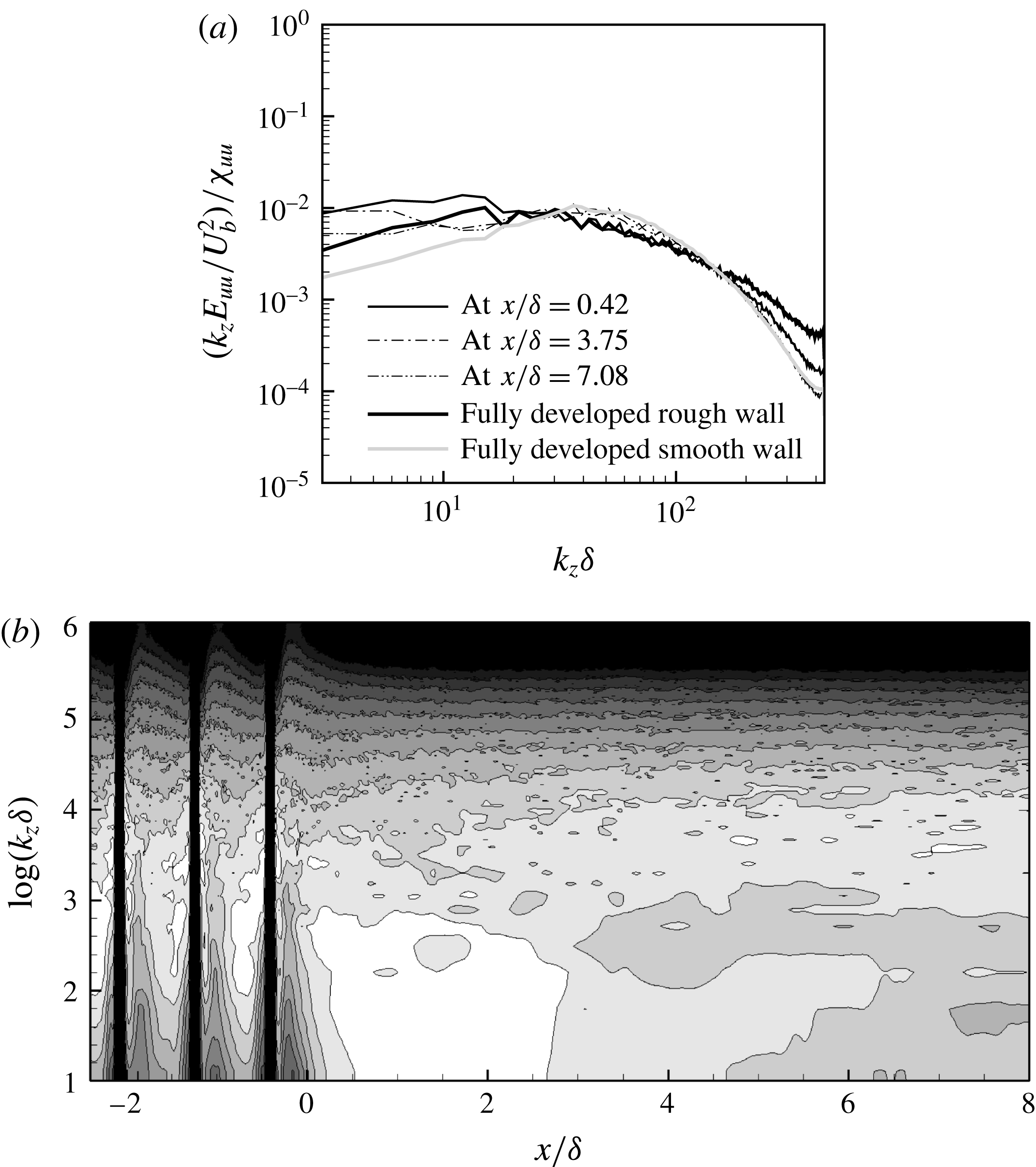
Normalized, premultiplied spanwise energy spectra at
 $y/\unicode[STIX]{x1D6FF}=0.023$
for case B. (a)
 $(k_{z}E_{uu}/U_{b}^{2})/\unicode[STIX]{x1D712}_{uu}$
at discrete streamwise stations. The fully developed rough-wall profile is located at
 $x/\unicode[STIX]{x1D6FF}=0$
. (b)
 $(k_{z}E_{uu}/U_{b}^{2})/\unicode[STIX]{x1D712}_{uu}$
in the continuous domain. Scale: white
 $10^{-2}$
, black
 $5(10^{-4})$
. The vertical lines for
 $x<0$
in (b) indicate the location of the roughness elements.

The near-wall energy spectra of turbulence fluctuations allow the recovery at small and at large scales of turbulence to be distinguished. The near-wall behaviour of premultiplied, energy spectra,
 $k_{z}E_{\unicode[STIX]{x1D6FC}\unicode[STIX]{x1D6FC}}(x,y)$
, as a function of spanwise wavenumber,
 $k_{z}$
, is shown in figure 21. For fully developed smooth-wall flow, the wall-normal location in this figure corresponds to
 $y^{+}\approx 20$
. To account for downstream decay of turbulence, at each streamwise station
 $k_{z}E_{\unicode[STIX]{x1D6FC}\unicode[STIX]{x1D6FC}}/U_{b}^{2}$
is normalized by
 $$\begin{eqnarray}\displaystyle & \displaystyle \unicode[STIX]{x1D712}_{\unicode[STIX]{x1D6FC}\unicode[STIX]{x1D6FC}}=\int _{0}^{2\unicode[STIX]{x03C0}N_{k}/L_{z}}\frac{k_{z}E_{\unicode[STIX]{x1D6FC}\unicode[STIX]{x1D6FC}}}{U_{b}^{2}}\,\text{d}(k_{z}\unicode[STIX]{x1D6FF}). & \displaystyle\end{eqnarray}$$
Here,
 $N_{k}$
is the total number of wavenumbers in the spanwise direction. On entering the transitional regime, the energy in the small scales shows the expected immediate drop, while at large scales there is an injection of energy. This is more clear from the white patch in the contour plot in figure 21(b). The initial increment of energy is attributed to downward reversion of the upward shifted turbulence structure over the rough wall. The intermediate scales exhibit slow downstream evolution, which in turn implies slow readjustment of the turbulence cascade near the developing smooth wall.
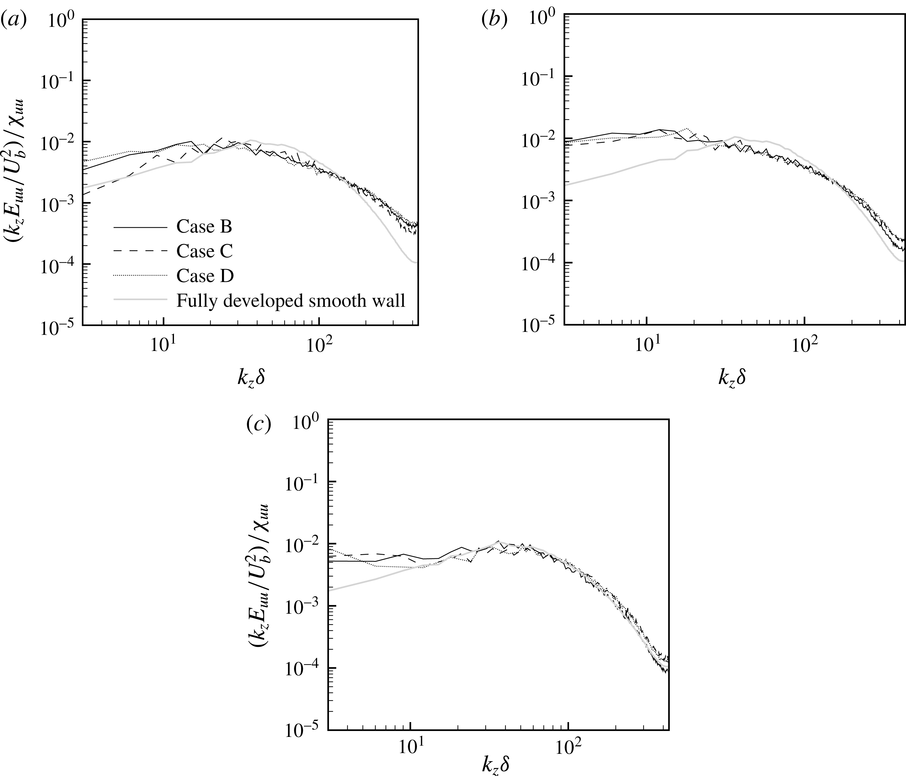
Normalized, premultiplied spanwise energy spectra,
 $(k_{z}E_{uu}/U_{b}^{2})/\unicode[STIX]{x1D712}_{uu}$
, at
 $y/\unicode[STIX]{x1D6FF}=0.023$
at (a)
 $x/\unicode[STIX]{x1D6FF}=0$
, (b)
 $x/\unicode[STIX]{x1D6FF}=0.42$
and (c)
 $x/\unicode[STIX]{x1D6FF}=7.08$
.

To compare the spectral recovery among different cases, profiles at fixed streamwise stations (
 $x/\unicode[STIX]{x1D6FF}$
) are plotted in figure 22. For intermediate and large wavenumbers
 $(k_{z}\unicode[STIX]{x1D6FF}>30)$
, a reasonable collapse is observed. The recovery at these intermediate and small scales thus progresses very similarly for all roughness cases considered here. Nonetheless, further studies with different roughnesses are needed to shed more light on the matter.
Energy spectra,
 $E_{uu}/U_{b}^{2}$
, as a function of spanwise wavenumber for case B (a) at
 $y/\unicode[STIX]{x1D6FF}=0.1$
and (b) at
 $y/\unicode[STIX]{x1D6FF}=1.0$
. —— at
 $x/\unicode[STIX]{x1D6FF}=-1.67$
, – – – at
 $x/\unicode[STIX]{x1D6FF}=0.42$
, – ⋅ – ⋅ – at
 $x/\unicode[STIX]{x1D6FF}=3.75$
, and
 $\cdots \cdots$
from smooth-wall channel flow.

 $E_{uu}/U_{b}^{2}=A(k_{z}\unicode[STIX]{x1D6FF})^{-5/3}$
.

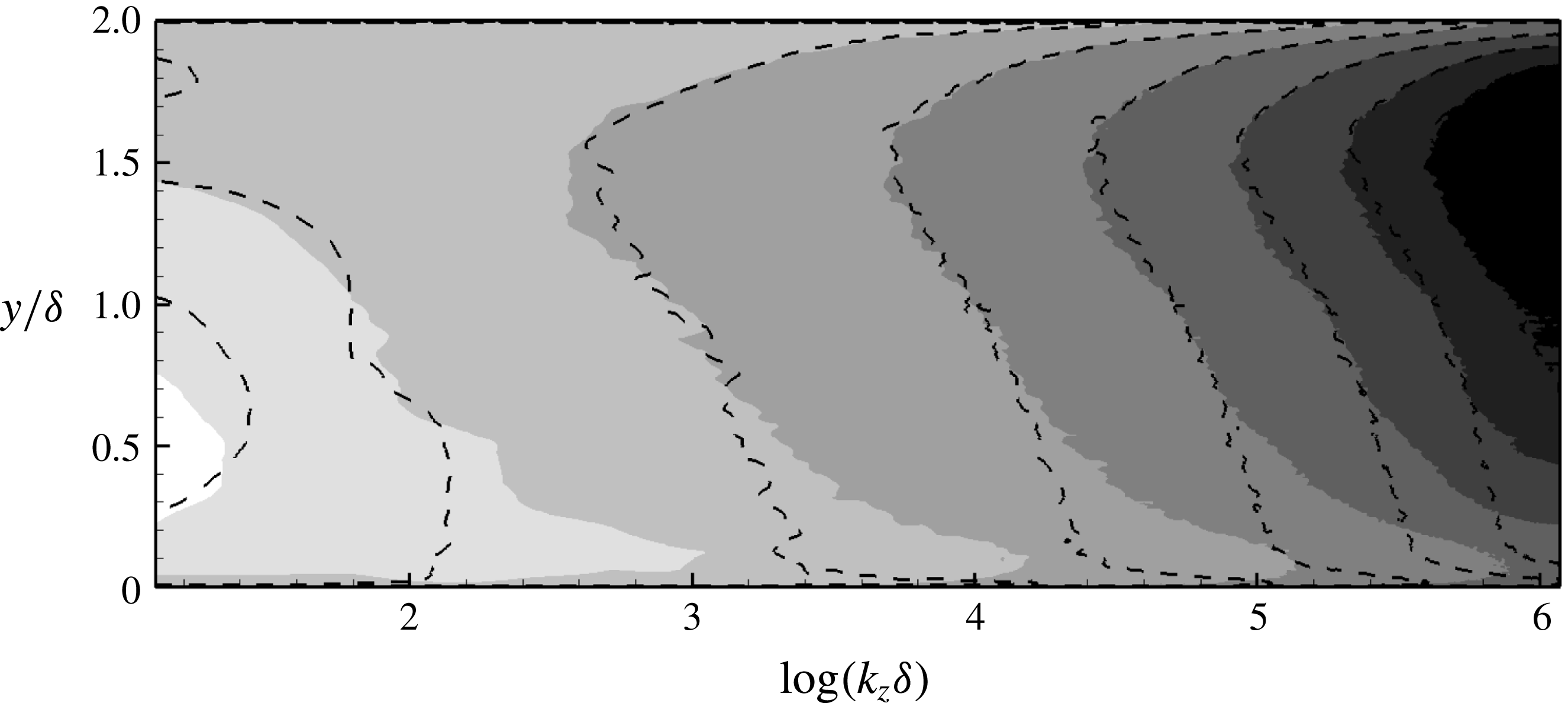
Wall-normal distribution of spanwise energy spectra,
 $E_{uu}/U_{b}^{2}$
, for case B. Greyscale contours: at
 $x/\unicode[STIX]{x1D6FF}=-1.67$
, and dashed lines: at
 $x/\unicode[STIX]{x1D6FF}=3.75$
. Scale: white 0.02, black
 $10^{-8}$
.

Figure 23 shows the energy spectra,
 $E_{uu}/U_{b}^{2}$
, as a function of the spanwise wavenumber at different streamwise locations and two wall-normal heights. The
 $k_{z}^{-5/3}$
scaling is clearly established, both near the wall, at
 $y/\unicode[STIX]{x1D6FF}=0.1$
in figure 23(a), and at the channel centreline in figure 23(b). There is a sharp reduction in energy at large wavenumbers, but clearly not as severe as seen in figure 21, at
 $y/\unicode[STIX]{x1D6FF}=0.023$
. The channel centreline shows negligible spectral recovery at large wavenumbers, which agrees with the results of
 $\unicode[STIX]{x1D716}$
from figure 20. The wall-normal dependence of energy spectra is plotted in figure 24 for two streamwise locations. Little change occurs with downstream distance near the upper smooth wall. However, close to the lower wall, at approximately
 $y/\unicode[STIX]{x1D6FF}<0.4$
, significant reduction in energy is observed. This reduction is broadband and a direct result of the removal of roughness. The decrease in energy is particularly intense at small wavenumbers; these small wavenumbers also show an increase in the spanwise length scale. At large wavenumbers and near the channel centre, the asymmetry in the wall-normal distribution of energy persists. This trend is consistent with the downstream relaxation of
 $\unicode[STIX]{x1D716}$
in figure 20(a,b).
The spectra highlight that very close to the wall, at
 $y^{+}=20$
, the rough-wall induced fine-scale motion quickly disappear once the roughness is removed. At large scales, however, there is an initial increase in the energy due to the turbulence which was displaced upward by the roughness, and which shifts downwards on transitioning to the smooth section. The expected streamwise decay follows, after this initial increase. Like the results of other turbulence quantities presented earlier, e.g.
 $\overline{u_{i}^{\prime }u_{j}^{\prime }}$
and
 $\unicode[STIX]{x1D716}$
, the recovery over the entire wavenumber range progresses quickly near the wall relative to a slow recovery in the outer flow.
3.7 Instantaneous visualizations
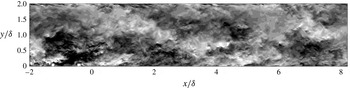
Figure 25 is a side view of the instantaneous streamwise velocity fluctuations, for a portion of the RTS regime. A fully developed smooth wall is characterized by intermittent, low-intensity eddies, that diffuse into the outer flow. This is in contrast to a rib-roughened wall, which is highly active and shows large-scale structures, of several rib spacings in length, above the roughness, along with much stronger, three-dimensional eddies, being created by the roughness elements (figure 1). Instantaneously, the size of these large-scale structures can vary between three and less than one rib spacings. Such large structures are seen in figure 25 for
 $x/\unicode[STIX]{x1D6FF}\lesssim 1$
,
 $y/\unicode[STIX]{x1D6FF}\lesssim 1$
. Figure 1 also shows these large structures above the roughness in the form of three separate white patches with streamwise size of approximately 2 rib spacings. The origin of these structures is uncertain; they seem to emerge from an interaction between the underlying roughness and the flow above it. Preliminary visualizations from RTS simulations using cube-roughened walls (not presented here) also support the presence of large-scale structures above the roughness, albeit of comparatively smaller size and weaker intensity. The turbulence statistics for these cube-roughened walls, however, including the mean velocity and turbulence stresses, are qualitatively quite similar to the results presented here.
Instantaneous streamwise velocity fluctuations
 $u^{\prime }$
in the
 $xy$
-plane for case B. Scale: white
 $+0.3$
, black
 $-0.3$
.

Instantaneous streamwise velocity fluctuations
 $u^{\prime }$
in the
 $xz$
-plane for case B at
 $y/\unicode[STIX]{x1D6FF}=0.023$
. (a) at
 $tU_{b}/\unicode[STIX]{x1D6FF}=t_{1}$
, and (b) at
 $tU_{b}/\unicode[STIX]{x1D6FF}=t_{1}+8.2$
. Scale: white
 $+0.2$
, black
 $-0.2$
. The vertical lines for
 $x<0$
indicate the location of the roughness elements.

Instantaneous streamwise velocity fluctuations
 $u^{\prime }$
in the
 $xz$
-plane for case B at
 $y/\unicode[STIX]{x1D6FF}=0.108$
. This wall-normal location corresponds to
 $y^{+}\approx 100$
in a fully developed smooth-wall channel flow. Scale: white
 $+0.3$
, black
 $-0.3$
.

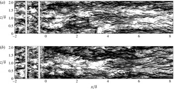
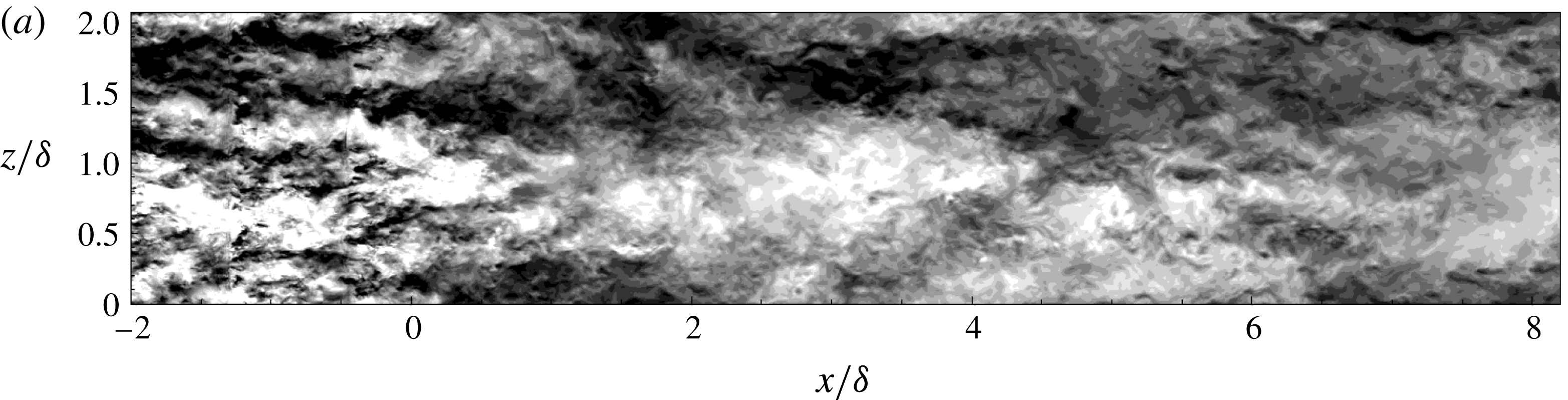
The impact of the upstream rough wall on qualitative recovery of the near-wall large-scale turbulence structure is more apparent from the
 $xz$
-plane visualizations of instantaneous
 $u^{\prime }$
in figure 26. The wall-normal height for these
 $xz$
-planes lies within the buffer layer and corresponds to
 $y^{+}\approx 20$
in fully developed smooth-wall flows. At this wall-normal height, the rough-wall zone contains high-intensity fluctuations, of small length and time scales. After RTS transition, however, there is an immediate reversion towards much larger length scales that are evident as early as
 $x/\unicode[STIX]{x1D6FF}\approx 0.5$
in figure 26. Much stronger, and larger turbulence structures continue to hinder the near-wall structural recovery and intermittently perturb the familiar high-speed and low-speed streaks, which are characteristic of fully developed smooth walls (Durbin & Reif Reference Durbin and Reif2011). As mentioned earlier, these large-scale structures are an injection of turbulence that had shifted upwards over the rough wall, and now reverts downwards. Figure 27 shows an instantaneous
 $u^{\prime }$
snapshot in the
 $xz$
-plane just above the roughness elements, at
 $y/\unicode[STIX]{x1D6FF}=0.108$
. This wall-normal location is characterized by large structures with spanwise size of the order of approximately one rib spacing, that show slight thickening after the RTS transition. This is indicated by the large white patch forming at
 $x/\unicode[STIX]{x1D6FF}\approx 3$
and
 $z/\unicode[STIX]{x1D6FF}\approx 1$
in figure 27. The spanwise enlargement of turbulence structure is coupled with the expected reduction in turbulence intensity, which is reflected by the contours becoming less distinct.
Further evidence for presence of these wider turbulence structures in the developing regime, is provided by the integral of spanwise two-point correlations,
 $R_{\unicode[STIX]{x1D6FC}\unicode[STIX]{x1D6FC}}^{z}$
, in figure 3. Compared to the rough wall, the developing smooth wall at
 $x/\unicode[STIX]{x1D6FF}=5$
in figure 3 shows a significant increase in the spanwise integral length scale, for all three fluctuating velocities.
Variation of the streamwise integral length scale,
 $L_{uu}$
, in the vicinity of step change in roughness for case B in the wall-normal direction. —— at
 $x/\unicode[STIX]{x1D6FF}=-0.55$
, —— at
 $x/\unicode[STIX]{x1D6FF}=-0.21$
, – – – at
 $x/\unicode[STIX]{x1D6FF}=0.49$
, – ⋅ – ⋅ – at
 $x/\unicode[STIX]{x1D6FF}=1.18$
,
 $\cdots \cdots$
at
 $x/\unicode[STIX]{x1D6FF}=1.88$
, — ⋅ ⋅ — at
 $x/\unicode[STIX]{x1D6FF}=2.57$
,


As also shown in figure 28, immediately after the RTS transition, there is a sharp increase in the streamwise integral length scale of
 $u^{\prime }$
fluctuations,
 $L_{uu}$
, for
 $y/\unicode[STIX]{x1D6FF}\lesssim 0.2$
. The streamwise integral length scale,
 $L_{uu}$
, for our RTS simulations is calculated by identifying the first minimum in the correlation curve for
 $R_{uu}^{x}$
and then calculating the integral up to this minimum. The near-wall streamwise structures immediately after the step change in roughness, that are influenced by large scales above the rough wall, are larger than their fully developed counterparts. As mentioned previously, these rough-wall large scales have a streamwise extent of approximately
 $1.5\unicode[STIX]{x1D6FF}$
(or approximately two rib spacings).
After the RTS transition, near the wall the reversion to much stronger mean shear (see figures 4
b and 9) results in quick re-emergence of the characteristic smooth-wall streaky structure. However, this strong mean shear near the wall does not prevent the large rough-wall structures from sporadically influencing the elongated streaks. Furthermore, further out, the weaker mean shear fails to effectively break up the large structures, which results in them continuing downstream. This, in addition to figure 28, can also be seen from figure 25 in the form of black patches continuing in the developing regime at approximately
 $y/\unicode[STIX]{x1D6FF}\approx 0.8$
.
4 Summary and conclusions
The development of a fully developed, rib-roughened turbulent channel flow, proceeding a over a smooth wall, has been studied by direct numerical simulations. These numerical experiments are the first of this configuration. Both statically averaged data and instantaneous visualizations have been discussed. The parameter
 $\unicode[STIX]{x1D6FF}/k$
is kept larger than most previous fully developed rough-wall simulations. All four test cases fall in the fully rough regime,
 $r^{+}>90$
.
The initial, fully developed regime generates realistic turbulent inflow conditions for the subsequent transitional regime, and is long enough to effectively break up the large structures. A long rough-wall region is necessary to minimize the contamination of large-scale statistics like
 $\overline{u^{\prime }u^{\prime }}$
over the developing smooth wall.
After the RTS transition, the skin friction,
 $C_{f}$
, shows a sharp reduction before recovering quickly and virtually levelling off by
 $x\approx 2\unicode[STIX]{x1D6FF}$
. Even so, reversion to fully developed magnitudes fails to occur. The mean velocity and Reynolds stress profiles show a slow recovery; by the last streamwise station, at
 $x/\unicode[STIX]{x1D6FF}=7.08$
, considerable mismatch with the symmetric, smooth-wall channel flow profiles remains. Extrapolations are provided that recovery might occur after
 $x\approx 40\text{ to }55\unicode[STIX]{x1D6FF}$
. Since the effect of step change in roughness is spread across the whole wall-normal extent of the channel, the traditional concept of an internal boundary-layer height does not apply. An equilibrium log layer, also, does not develop within the domain. From mean-velocity and skin-friction viewpoints, the transitional regime could be divided roughly into two zones: an initial strong non-equilibrium zone within
 $0<x/\unicode[STIX]{x1D6FF}<0.5$
, followed by a weak non-equilibrium zone from
 $x/\unicode[STIX]{x1D6FF}>0.5$
. In the near-wall region of the strong non-equilibrium zone (see figure 11
b),
 $\overline{U}^{+}$
increases with downstream distance, while the opposite trend is observed farther from the wall. This is a consequence of strong variation in
 $C_{f}$
immediately after the RTS transition.
By the end of the computational domain, turbulence stresses still show a strong mismatch with smooth-wall channel flow results, except in a thin layer very close to the wall. Above the thin wall layer, much higher turbulence persists throughout. It is carried downstream from the upstream, rough wall. From normalized recovery magnitudes (
 $\unicode[STIX]{x1D6FD}_{ij}$
) and quadrant analysis, it is evident that the shear-stress producing motions recover more quickly than large structures associated with
 $\overline{u^{\prime }u^{\prime }}$
above the thin, wall layer. Gradients of momentum fluxes, that are influenced by the roughness size, contribute significantly to the overall momentum balance, and this balance is not just between pressure gradient and shear stress – as in fully developed regimes.
The rough wall creates a high dissipation rate,
 $\unicode[STIX]{x1D716}$
. In the transitional regime, upon removal of the roughness elements,
 $\unicode[STIX]{x1D716}$
decays rapidly. But by the end of the computational domain,
 $\unicode[STIX]{x1D716}$
is still approximately
 $50\,\%$
higher than the equilibrium smooth-wall level. The higher
 $\unicode[STIX]{x1D716}$
results in a smaller turbulence time scale,
 $K/\unicode[STIX]{x1D716}$
, persisting over the smooth wall.
Instantaneous visualizations of
 $u^{\prime }$
contours display the presence of large structures, of several ribs spacings in size, above the rough wall. These large structures continue downstream into the transitional regime, except for reverting downwards. They influence the near-wall structural recovery. Evidence for these large structures is also provided by the spanwise energy spectra in figure 21 and by the streamwise integral length scale in figure 28. Elongated streaks appear promptly after the RTS transition, but they are being intermittently perturbed by the ambient large structures.
Acknowledgements
This work was supported by the Office of Naval Research under award no. N00014-17-1-2200 and by the US Army under contract no. W911W6-14-C-0003. Computational resources were provided by NASA’s High-End Computing (HEC) section under award nos ARMD-15-6415, ARMD-16-7597 and ARMD-18-8100.