2. The ALPS algorithm

Tempering methods for MCMC usually consider powers $\pi^\beta$ for small values $\beta \in (0,1]$ , to make the target distribution flatter and thus allow for easier mixing between modes. By contrast, [Reference Tawn, Moores and Roberts29] introduces the ALPS algorithm, which instead uses large values $\beta \gg 1$ , combined with locally weight-preserving tempering distributions as in [Reference Tawn, Roberts and Rosenthal31] so the modes retain their relative masses. These choices make the modes of $\pi$ even more separated. However, under certain smoothness and integrability assumptions, they also make each mode appear approximately Gaussian and hence similarly shaped. This allows for auxiliary ‘mode-jumping’ Markov chain steps which move effectively between the different modes when $\beta$ is large. Then, as usual, only samples in the original temperature $\beta=1$ are ‘counted’ as actual samples from $\pi$ .

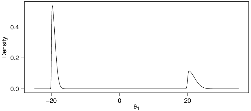
To illustrate the idea of this algorithm, consider the following simple example in dimension $d=5$ . Suppose the target density $\pi$ on ${\mathbb R}^5$ is a mixture of two skew-normal modes centered at $(\!-20,-20,-20,-20,-20)$ and (20, 20, 20, 20, 20) respectively, with scalings 1 and 2 respectively, and with shape parameter $\alpha=10$ ; so, for all $\theta\in{\mathbb R}^5$ ,

\begin{equation*}\pi(\theta) =(0.7) \prod_{i=1}^5 2 \, \phi\big( \theta_i+20 \big) \, \Phi\big( 10(\theta_i+20) \big) +(0.3) \prod_{i=1}^5 \phi\big( \tfrac{1}{2}(\theta_i-20) \big) \, \Phi\big( 5(\theta_i-20) \big) ,\end{equation*}

where as usual $\phi(x) = \frac{1}{\sqrt{2\pi}\,} \textrm{e}^{-x^2/2}$ and $\Phi(x) = \int_{-\infty}^x \phi(u) \, \textrm{d} u$ ; see Figure 1.

Figure 1.

The $\theta_1$ marginal of the target density in the illustrative example.

In such an example, it is very easy for a Markov chain to mix separately within either of the two modes. The challenge is to move between the modes (which is virtually impossible for a typical fixed-temperature Metropolis algorithm even in this simple five-dimensional example). 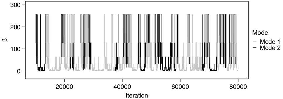The ALPS algorithm introduces a powerful independence-sampler-based move so that at very large inverse-temperature values $\beta \gg 1$ , the chain can exploit the near-Gaussianity of each of the modes to directly jump between them. Figure 2 shows a trace plot of the inverse temperature values $\beta$ during one run of the algorithm, and also indicates by colour which of the two modes the chain is in (i.e. closest to). As can be seen from the plot, the chain stays in the same mode for long periods of time, and only switches modes when the values of $\beta$ are very large, at which point it jumps to either mode with its correct probability. (Note that this description is for the ‘vanilla’ version of ALPS; see Remark 1.)

Figure 2.

Trace plot of the $\beta$ values in the illustrative example, coloured to indicate whether the chain is in mode 1 (light-grey) or mode 2 (black).

Figure 2 illustrates that the key to the ALPS algorithm’s success is moving rapidly between the large $\beta= \beta_\textrm{max} = 256$ values (which allow for mixing between the modes) and the small $\beta=1$ value (which can be ‘counted’ as a sample from $\pi$ ). However, it is not clear how quickly such mixing takes place, and in particular how it changes depending on the target $\pi$ and dimension d. To study this, we would like to prove a diffusion limit of a suitably scaled version of the $\beta$ process, but it is not clear from Figure 2 what sort of limiting diffusive behaviour is available.

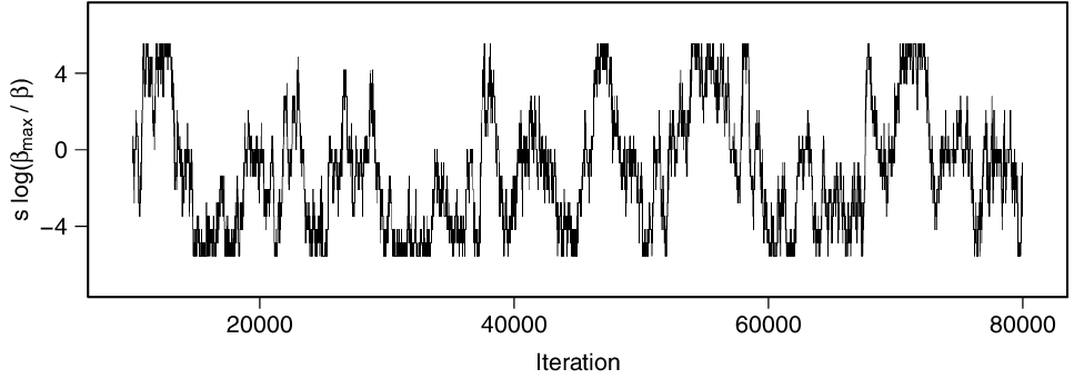
To better understand this algorithm’s convergence, we consider a suitable transformation of $\beta$ . Namely, we instead consider the values of $s \log(\beta_\textrm{max}/\beta)$ , where $s=1$ if the chain is in mode 1 or $s=-1$ if the chain is in mode 2. The resulting process is shown in Figure 3, which suggests that this modified functional does indeed start to resemble a diffusive process. Indeed, away from the special value 0 (corresponding to $\beta_\textrm{max}$ and the mode-jumping moves), the process looks roughly like Brownian motion. In fact, we prove in Theorem 3 that under appropriate assumptions and scalings, this modified process converges to a skew Brownian motion.

Figure 3.

A trace plot of the transformed values $s \log(\beta_\textrm{max}/\beta)$ in the illustrative example, where $s=+1$ or $s=-1$ when the chain is in mode 1 or 2.

More precisely, we shall prove diffusion limits for suitably rescaled versions of the ALPS algorithm, as the dimension $d\to\infty$ . We shall assume that the ALPS algorithm can easily jump between modes when it reaches the sufficiently large inverse temperature $\beta_\textrm{max}^{(d)}$ , but that it is stuck within one mode whenever $\beta < \beta_\textrm{max}^{(d)}$ . We therefore focus on how the inverse temperatures $\beta$ themselves are updated by the algorithm. In particular, we prove in Theorem 3 that a particular rescaling of the $\beta$ process converges to skew Brownian motion [Reference Lejay14]. This in turn allows us to derive computational complexity results (Section 5).

3. Assumptions

We consider a version of the ALPS algorithm of [Reference Tawn, Moores and Roberts29]. We assume the chain always mixes immediately within each mode, but the chain can only jump between modes when at the sufficiently cold inverse temperature $\beta = \beta_\textrm{max}^{(d)}$ , at which point it immediately jumps to any of its modes with the correct probability weight.

To facilitate theoretical analysis, we assume that the target density $\pi$ is a mixture of J normalised densities $g_1,\ldots,g_J$ on ${\mathbb R}^d$ with weights $w_1,\ldots,w_J$ , i.e.

(1) \begin{equation}\pi(x) = \sum_{j=1}^J w_j g_j(x) , \qquad x\in{\mathbb R}^d . \end{equation}

We do not require the $g_j$ to be unimodal, but we shall nevertheless refer to them informally as the ‘modal components’ or ‘modes’ of $\pi$ , with the intuition that it is easy for MCMC to mix efficiently within each individual $g_j$ but difficult for it to jump between the different $g_j$ .

We also assume that each state x is ‘allocated’ to (i.e. is ‘in’) one of the modes (e.g. whichever one’s centre it is closest to), such that the accept/reject probabilities when updating $\beta$ can be computed using only the mode $g_j$ of the current state, rather than the full density $\pi$ .

(This corresponds to considering the x values as elements of $\big({\mathbb R}^d\big)^J$ , with a different version of the state space ${\mathbb R}^d$ for each of the J modes; if the modes are well separated then, especially for large $\beta$ , this will be a good approximation to the actual algorithm.)

Then, for each inverse temperature $\beta \ge 1$ we use the tempered distribution

(2) \begin{equation}\pi_\beta(x) \propto\sum_{j=1}^J w_j \frac{[g_j(x)]^\beta}{\int [g_j(x)]^\beta \, \textrm{d} x} \,{=\!:}\,\sum_{j=1}^J w_j \, g_j^\beta(x) ,\end{equation}

where $g_j^\beta$ are the normalised powers of the $g_j$ . We assume the same weights $w_j$ can be used for each $\beta$ due to a weight-preserving transformation as in [Reference Tawn, Roberts and Rosenthal31].

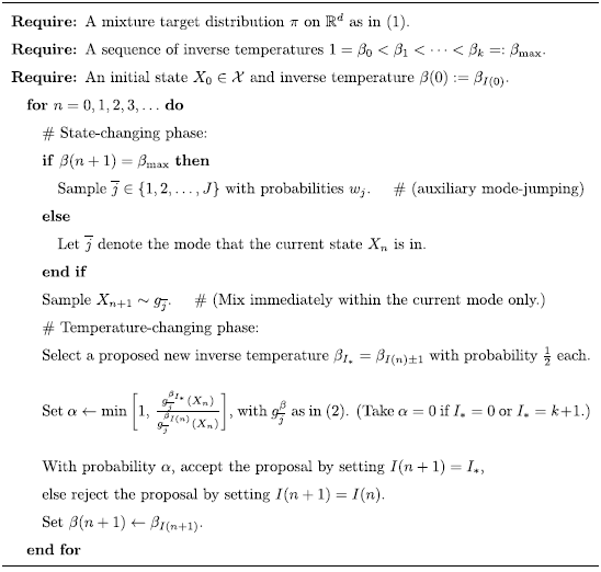
In terms of these assumptions, the vanilla ALPS algorithm as we shall study it is defined by Algorithm 1.

Algorithm 1:

The vanilla ALPS algorithm.

In our theoretical proofs below, we assume for simplicity (though see Remark 3) that we have just $J=2$ modes, of weights $w_1$ and $w_2=1-w_1$ . To achieve limiting diffusions, we further assume, as in the original MCMC diffusion limit results [Reference Roberts, Gelman and Gilks21], that each of the individual components $g_j$ consists of i.i.d. univariate coordinates, i.e. that, for each j, we have

(3) \begin{equation}g_j(x) = \prod_{i=1}^d \overline{g}_j(x_i)\end{equation}

for some fixed one-dimensional density function $\overline{g}_j$ , where $x=(x_1,x_2,\ldots,x_d)$ . This allows us to apply the diffusion limit results of [Reference Roberts and Rosenthal25] within each individual target mode. (Although (3) is a very restrictive assumption, it is known [Reference Roberts and Rosenthal23] that conclusions drawn from this special case are often approximately applicable in much broader contexts.)

We also require assumptions on the $\beta$ values. Write the inverse temperatures as

(4) \begin{equation}1 = \beta_0^{(d)} < \beta_1^{(d)} <\cdots < \beta^{(d)}_{k(d)} \,{=\!:}\, \beta_\textrm{max}^{(d)}\end{equation}

for the process in dimension d. Similar to [Reference Atchadé, Roberts and Rosenthal2, Reference Roberts and Rosenthal25], following [Reference Predescu, Predescu and Ciobanu19, Reference Kone and Kofke13], we assume that the inverse temperatures are related by

(5) \begin{equation}\beta_i = \beta_{i-1} +\ell(\beta_{i-1})/d^{1/2}\end{equation}

for some fixed $C^1$ function $\ell$ . It is shown in [Reference Atchadé, Roberts and Rosenthal2, Reference Roberts and Rosenthal25] that in the single-mode i.i.d. case, the fastest limiting diffusion is obtained by using the choice

(6) \begin{equation}\ell(\beta) = I^{-1/2}(\beta) \, \ell_0\end{equation}

for a fixed constant $\ell_0 \doteq 2.38$ , where $I(\beta) = {\rm Var}_{x \sim \overline{g}^\beta}(\log \overline{g}(x))$ . Inspired by this, in our later results we assume the proportionality condition that the quantities $I_j(\beta) \,{:\!=}\, {\rm Var}_{x \sim \overline{g}_j^\beta}(\log \overline{g}_j(x))$ for the different modes are proportional, i.e. there are positive constants $r_j$ and a $C^1$ function $I_0 \,{:}\, \mathbb{R}_{+}\to\mathbb{R}_{+}$ such that

(7) \begin{equation}I_j(\beta) = I_0(\beta)/r_j , \qquad j=1,\ldots,J ,\end{equation}

and shall then correspondingly assume that

(8) \begin{equation}\ell(\beta) = I_0^{-1/2}(\beta) \, \ell_0\end{equation}

for some fixed constant $\ell_0>0$ .

One example is the exponential power family case, in which each of the mixture component factors $g_j$ is of the form $g_j(x) \propto \textrm{e}^{-\lambda_j|x|^{r_j}}$ for some $\lambda_j,r_j>0$ . It then follows from [Reference Atchadé, Roberts and Rosenthal2, Section 2.4] that $I_j(\beta) = \beta^{-2}/r_j$ for $\beta>0$ , so the proportionality condition (7) holds with $I_0(\beta)=\beta^{-2}$ . The corresponding choice of $\ell$ from (6) is then $\ell(\beta) = \beta/\sqrt{r_j}$ in mode j. This includes the Gaussian case, where each $r_j=2$ and $\lambda_j = 1/\sigma_j^2$ .

4. Main results

We now state various weak convergence results for various transformations of our process. (All proofs are deferred to Section 6.) Let $\beta^{(d)}(t)$ be the inverse temperature at time t for the process described by Algorithm 1 in dimension d. Let $\beta^{(d)}(N(dt))$ be a continuous-time version of the $\beta^{(d)}(t)$ process, sped up by a factor of d, where $\{N(t)\}$ is an independent standard rate-1 Poisson process. To combine the two modes into one single process, we further augment this process by multiplying it by $-1$ when the algorithm’s state is allocated to the second mode, while leaving it positive (unchanged) when state is allocated to the first mode, i.e.

(9) \begin{equation} X_t^{(d)} = \begin{cases} \beta^{(d)}({N(dt)}) & \textrm{in mode 1} , \\[3pt] - \beta^{(d)}({N(dt)}) \quad & \textrm{in mode 2} . \\ \end{cases}\end{equation}

Our first diffusion limit result, following [Reference Roberts and Rosenthal25], states that within each mode, the inverse temperature process behaves identically to the case where there is only one mode (i.e. $J=1$ ). To state it, we extend the definition of I to

(10) \begin{equation} I(\beta) = \begin{cases} {\rm Var}_{x\sim f_1^\beta}(\log f_1(x)) , & \beta>0 , \\[3pt] {\rm Var}_{x\sim f_2^{|\beta|}}(\log f_2(x)) , \quad & \beta<0 . \\ \end{cases}\end{equation}

Theorem 1. Assume the target distribution $\pi$ is of the form (1), with $J=2$ modes of weights $w_1$ and $w_2=1-w_1$ , each having i.i.d. coordinates as in (3), with tempered distributions as in (2) for an inverse-temperatures list (4) related by (5). Then, away from its boundary points 1 and $\beta_\textrm{max}^{(d)}$ , the process $\big\{X_t^{(d)}\big\}$ from (9) converges weakly as $d\to\infty$ to a fixed diffusion process X, which for $X^{(d)}>0$ satisfies

(11) \begin{align} \textrm{d} X_t &= \bigg[2 \ell^2(X_t) \, \Phi\bigg( \frac{- \ell(X_t) I^{1/2}(X_t)}{2} \bigg) \bigg]^{1/2} \textrm{d} B_t \nonumber\\[3pt] &\qquad\qquad\quad\qquad + \bigg[\ell(X_t) \, \ell'(X_t) \ \Phi \bigg(\frac{-I^{1/2}(X_t) \ell(X_t)}{2}\bigg)\nonumber\\[3pt] &\qquad\qquad\quad\qquad\qquad - \ell^2(X_t) \bigg(\frac{\ell(X_t) I^{1/2}(X_t)}{ 2} \bigg)' \phi \bigg( \frac{-I^{1/2}(X_t) \ell(X_t)}{2} \bigg) \bigg] \textrm{d} t . \end{align}

The same equation holds for $X_t<0$ , except with the sign of the drift reversed.

As a check, (11) satisfies the general relation $\mu(x)= \tfrac{1}{2} \sigma^2(x)\frac{\textrm{d}}{{\textrm{d} x}} \log \pi(x) + \sigma(x) \sigma'(x)$ , which implies that $\pi$ is locally invariant for $X^{(d)}$ , i.e. that its generator G has $\pi (G f)(x) = 0$ for appropriate smooth f and for x in the interior of the domain. That is, $\pi$ is stationary for $X^{(d)}$ locally within each mode, as expected.

However, Theorem 1 describes only what happens on each mode separately; it says nothing about the mode-jumping process itself. Moreover, its state space $(\!-\infty,-1]\cup [1,\infty)$ is not connected. In fact, we will see that as $d\to\infty$ , the value $\beta_\textrm{max}^{(d)}$ will go to infinity and hence never be reached in finite time. To resolve these issues, we make several transformations on the $X^{(d)}_t$ process. First, for $|x| \ge 1$ , we define $h(x) = \int_1^{|x|} \frac{1}{\ell (u)} \, \textrm{d} u$ . (For example, in the exponential power family case, $I(\beta) \propto 1/\beta^2$ , so (8) gives $\ell(\beta) = I_0^{-1/2}(\beta) \, \ell_0 \propto \beta$ , whence $h(x) = \int_1^{|x|} \frac{1}{\ell(u)} \, \textrm{d} u\propto \int_1^{|x|} \frac{1}{u} \, \textrm{d} u= \log|x|$ .) We then set

(12) \begin{equation}H_{t (h(\beta_\textrm{max}^{(d)}))^2}^{(d)} ={\rm sign}\left(X_{t h(\beta_\textrm{max}^{(d)})^2}^{(d)}\right) \left[ 1 + \frac{h\left( X^{(d)}_{t h(\beta_\textrm{max}^{(d)})^2} \right)}{h(\beta_\textrm{max}^{(d)})} \right] .\end{equation}

Hence, $1 \le H_t^{(d)} \le 2$ in the first mode, and $-1 \ge H_t^{(d)} \ge -2$ in the second mode. Also, $H_t^{(d)}$ speeds up $X_t^{(d)}$ by a factor of $h\big(\beta_\textrm{max}^{(d)}\big)^2$ , and hence moves at Poisson rate $d h\big(\beta_\textrm{max}^{(d)}\big)^2$ . This new process $H_t^{(d)}$ satisfies the following.

Theorem 2. Under the set-up and assumptions of Theorem 1, on $(\!-2,-1) \cup (1,2)$ (i.e. away from its boundary points), the process $\big\{H_t^{(d)}\big\}$ from (12) converges weakly in the Skorokhod topology as $d\to\infty$ to a limiting diffusion H which satisfies

(13) \begin{equation}\textrm{d} H_t = \left[ 2 \Phi\left( \frac{- \ell(X_t) I^{1/2}(X_t)}{2} \right) \right]^{1/2} \textrm{d} B_t+ \ell(X_t) \bigg[ \Phi \bigg( \frac{-I^{1/2}(X_t) \ell(X_t)}{2} \bigg) \bigg]^{\prime} \textrm{d} t .\end{equation}

Furthermore, H leaves constant (uniform) densities locally invariant.

To make further progress, we now use the proportionality condition (7), with corresponding inverse-temperature spacing (8). It then follows from the extended definition (10) that $\ell(X_t) \, I^{1/2}(X_t) = \ell_0 r_1^{1/2}$ for $X_t < 0$ , and $\ell(X_t) \, I^{1/2}(X_t) = \ell_0 r_2^{1/2}$ for $X_t > 0$ , with $\big[ \ell(X_t) \, I^{1/2}(X_t) \big]' = 0$ for all $X_t \not= 0$ . Hence, Theorem 2 immediately gives the following corollary.

Corollary 1. Assume the set-up and assumptions of Theorem 1, and also the proportionality condition (7) with inverse-temperature spacing (8). Then, as $d\to\infty$ , the process $\big\{H_t^{(d)}\big\}$ converges weakly in the Skorokhod topology to a limit process H on $(\!-2,-1)$ and on (1,2), i.e. away from its boundary points. Furthermore, H is a diffusion, with drift 0, and with diffusion coefficient which is constant on each of the two intervals $(\!-2,-1)$ and (1,2). Specifically, $\textrm{d} H_t = s(H_t) \, \textrm{d} B_t$ , where $s(H_t) = s_1$ for $H_t \in (1,2)$ , and $s(H_t) = s_2$ for $H_t \in (\!-2,-1)$ , with

(14) \begin{equation}s_i \,{:\!=}\, \bigg[ 2 \Phi\left( - \tfrac{1}{2} \ell_0 r_i^{1/2} \right) \bigg]^{1/2} .\end{equation}

Next, we need to join up the two parts of the domain $[-2,-1] \cup[1,2]$ of the process $H_t^{(d)}$ . Now, the original process can jump between modes when at the coldest temperture $\beta_\textrm{max}^{(d)}$ , corresponding to the values $\pm 2$ for the transformed process $H_t^{(d)}$ . Hence, we let

(15) \begin{equation} Z_t^{(d)} = 2 {\rm sign}\big(H_t^{(d)}\big) - H_t^{(d)} = \begin{cases} 2 - H_t^{(d)} , & H_t^{(d)} \ge 1, \ \textrm{i.e. in mode 1} , \\[3pt] -2 - H_t^{(d)} , \quad & H_t^{(d)} \le -1, \ \textrm{i.e. in mode 2} , \\[3pt] \end{cases}\end{equation}

so that $Z_t^{(d)}$ has domain $[-1,1]$ with mode-jumping at 0.

However, by Corollary 1, the limit of the process $Z_t^{(d)}$ will still have diffusion coefficient $s_1$ or $s_2$ on its positive and negative parts. We thus rescale the process by setting

(16) \begin{equation}W^{(d)}_t = s(Z^{(d)}_t)^{-1} \, Z^{(d)}_t .\end{equation}

(So, to recap, $W_t^{(d)}$ is defined in (16) in terms of $Z_t^{(d)}$ , which is defined in (15) in terms of $H_t^{(d)}$ , which is defined in (12) in terms of $X_t^{(d)}$ , which is in turn defined in (9) in terms of the original inverse-temperature process $\beta^{(d)}(t)$ , which itself arises from running Algorithm 1.) Then, $W^{(d)}_t$ has domain $\Big[{-}\frac{1}{s_2},\frac{1}{s_1}\Big]$ , and a limit which is actual Brownian motion on each of $\Big({-}\frac{1}{s_2},0\Big)$ and $\Big(0,\frac{1}{s_1}\Big)$ . The precise limit of this process requires the notion of skew Brownian motion, a generalisation of usual Brownian motion that, intuitively, behaves just like a Brownian motion except that the sign of each excursion from 0 is chosen using an independent Bernoulli random variable; for further details, constructions, and discussion see, e.g., [Reference Lejay14]. In terms of skew Brownian motion, we have the following theorem.

The above theorems are all proved in Section 6. First, we use them to investigate the computational complexity of the ALPS algorithm.

5. Computational complexity

Theorem 3 has implications for the computational complexity of the ALPS algorithm. Indeed, it shows that the limiting process W does not depend at all on the dimension d, and hence has convergence time O(1) as $d\to\infty$ . However, W was derived from the processes $H_t^{(d)}$ and $Z_t^{(d)}$ , which sped up time by a factor of $\Big(h\big(\beta_\textrm{max}^{(d)}\big)\Big)^2$ from the process $X_t^{(d)}$ , which itself sped up time by a factor d. That is, W was sped up by a total factor of $d \Big[h\big(\beta_\textrm{max}^{(d)}\big)\Big]^2$ . So, in the original scaling, the convergence time is $O\Big(d \Big[h(\beta_\textrm{max}^{(d)})\Big]^2\Big)$ .

More formally, it is shown in [Reference Roberts and Rosenthal24, Theorem 1] that such diffusion limit convergence implies that for any $\epsilon>0$ , the convergence time $T_\epsilon$ for each component of the original process to get within $\epsilon$ of stationary in Kantorovich–Rubinstein distance, averaged over starting state chosen from stationarity, will be of the same order as the speedup factor. So, combining Theorem 3 and [Reference Roberts and Rosenthal24, Theorem 1] shows that, for the $\beta$ process of the vanilla ALPS algorithm, the convergence time $T_\epsilon$ is $O\big(d \big[h(\beta_\textrm{max}^{(d)})\big]^2\big)$ . Furthermore, this convergence time is indeed an appropriate measure of the algorithm’s efficiency, since it is proportional to the rate at which the $\beta$ values can complete a ‘round trip’ from one sample at $\beta=1$ , to a mode jump at $\beta=\beta_\textrm{max}$ , to another sample at $\beta=1$ , and hence mix well between modes; similar approaches appear in [Reference Atchadé, Roberts and Rosenthal2, Reference Jacka and Hernández-Hernández11, Reference Syed, Bouchard-Côté, Deligiannidis and Doucet28].

This raises the question of how $h\big(\beta_\textrm{max}^{(d)}\big)$ grows as a function of d. It is proved in [Reference Tawn, Moores and Roberts29] that for the ALPS process to mix modes efficiently, we need the maximum inverse temperature value $\beta_\textrm{max}^{(d)}$ to grow linearly with dimension, i.e. we need to choose $\beta_\textrm{max}^{(d)} \propto d$ . And, in the exponential power family case, as mentioned above, $I(\beta) \propto 1/\beta^2$ , which implies by (8) that $h(x) \propto \log|x|$ , so $h\big(\beta_\textrm{max}^{(d)}\big) \propto \log(d)$ . Hence, the complexity order $O\big(d \big[h(\beta_\textrm{max}^{(d)})\big]^2\big)$ equals $O\big(d [\log d]^2\big)$ . That is, for the inverse temperature process to hit $\beta_\textrm{max}^{(d)}$ and hence mix modes takes $O\big(d [\log d]^2\big)$ iterations.

If we are not in the exponential power family case, then it may no longer be true that $I(\beta) \propto 1/\beta^2$ . However, as $d,\beta\to\infty$ , under appropriate smoothness assumptions the densities in the different modes will become approximately Gaussian, which corresponds to the exponential power family case with $r=2$ . And, it is proved in [Reference Tawn and Roberts30, Equation (66)] that if the first four moments converge to those of a Gaussian, then $2\beta^2 I(\beta) \to 1$ , i.e. approximately $I(\beta) \propto 1/\beta^2$ . Hence, from (8), approximately $\ell(\beta) \propto \beta$ , so again $h\big(\beta_\textrm{max}^{(d)}\big) \propto \log(d)$ , and the complexity order is still $O\big(d [\log d]^2\big)$ as before. We summarise this conclusion as follows.

In a different direction, [Reference Tawn and Roberts30] introduces the QuanTA algorithm, which modifies parallel tempering’s usual temperature-swap moves by adjusting the x space in order to permit larger moves in the inverse temperature space. As a result of this, [Reference Tawn and Roberts30, Theorem 2] shows that the resulting $\ell(\beta)$ function is then proportional to $\beta^{k/2}$ for some $k>2$ (instead of proportional to $\beta$ ). In that case,

\begin{equation*}h\big(\beta_\textrm{max}^{(d)}\big) = \int_1^{\beta_\textrm{max}^{(d)}} \frac{1}{\ell(u)} \, \textrm{d} u \le \int_1^\infty \frac{1}{\ell(u)} \, \textrm{d} u \propto \int_1^\infty u^{-k/2} \, \textrm{d} u = (k/2) - 1 < \infty ,\end{equation*}

so that $h\big(\beta_\textrm{max}^{(d)}\big)$ is O(1) rather than $O(\log d)$ . This means that the convergence complexity $O\Big(d \Big[h\big(\beta_\textrm{max}^{(d)}\big)\Big]^2\Big)$ becomes simply O(d), i.e. the $[\log d]^2$ factor vanishes. We summarise this observation as follows.

Comparing Corollaries 2 and 3, we see that the QuanTA modification improves the complexity bound by a factor of $[\log d]^2$ . This is not surprising, since QuanTA was specifically designed to make the algorithm move faster, especially under near-Gaussianity at large $\beta$ , thus improving the mixing time. This improvement is also borne out through simulation experiments; see [Reference Tawn and Roberts30].

6. Theorem proofs

In this section we prove the theorems stated in Section 4. Note that Theorem 1 essentially follows directly from the previous theoretical analysis of simulated tempering in [Reference Atchadé, Roberts and Rosenthal2, Reference Roberts and Rosenthal25], and Theorem 2 then follows from some additional computations using Itô’s formula. By contrast, Theorem 3 requires a different approach, to show that the modified $W^{(d)}$ process converges to reflecting skew Brownian motion, including delicate arguments to show the convergence of the corresponding infinitesimal generators, especially at the two endpoints and at the excursion point 0.

6.2. Proof of Theorem 2

We assume $x\in(1,2)$ ; the proof for $x\in(\!-2,-1)$ is virtually identical. Here $H_t = h(X_t)$ , where $h'(x) = \ell(x)^{-1}$ , and $h''(x) = -\ell'(x) \ell(x)^{-2}$ . Hence, by Itô’s formula,

\begin{align*}\textrm{d} H_t& = h'(X_t) dX_t + \frac{1}{2} h''(X_t) d\langle X \rangle_t \\[3pt]& = \ell(X_t)^{-1} \textrm{d} X_t - \frac{1}{2} \ell'(X_t) \ell(X_t)^{-2}\textrm{d} \langle X \rangle_t \\[3pt]& = \ell(X_t)^{-1}\left[2 \ell^2(X_t) \Phi\left( \frac{- \ell(X_t) I^{1/2}(X_t)}{ 2} \right) \right]^{1/2} \textrm{d} B_t \\[3pt] & \quad + \ell(X_t)^{-1} \ell(X_t) \ell'(X_t) \Phi \left(\frac{-I^{1/2}(X_t) \ell(X_t)}{ 2}\right) \textrm{d} t \\[3pt] & \quad - \ell^2(X_t) \left(\frac{\ell(X_t) I^{1/2}(X_t)}{ 2} \right)' \phi \left( \frac{-I^{1/2}(X_t) \ell(X_t)}{ 2} \right) \textrm{d} t \\[3pt] & \quad - \frac{1}{2} \ell'(X_t) \ell(X_t)^{-2} 2 \ell^2(X_t) \Phi\left( \frac{- \ell(X_t) I^{1/2}(X_t)}{ 2} \right) \textrm{d} t .\end{align*}

In this last equation, the second and fourth terms cancel. Also, since $\Phi' = \phi$ , it follows from the chain rule that the third term can be written as

\begin{equation*}- \ell^2(X_t)\left[ \Phi \left( \frac{-I^{1/2}(X_t) \ell(X_t)}{ 2} \right) \right]^{\prime} \textrm{d} t .\end{equation*}

This gives (13). Then, writing everything in terms of $H_t = h(X_t)$ , this becomes

\begin{align*} \textrm{d} H_t & = \left[ 2 \, \Phi\left( \frac{- \ell(h^{-1}(H_t)) I^{1/2}(h^{-1}(H_t))}{2} \right) \right]^{1/2} \textrm{d} B_t \\[3pt] & \quad + \ell(h^{-1}(H_t)) \bigg[ \Phi \left( \frac{-I^{1/2}(h^{-1}(H_t)) \ell(h^{-1}(H_t))}{2} \right) \bigg]' \textrm{d} t .\end{align*}

Now, a diffusion of the form $\textrm{d} H_t = \sigma(H_t) \textrm{d} B_t +\mu(H_t) \textrm{d} t$ has locally invariant distribution $\pi$ provided that $\frac{1}{2} (\log\pi)' \sigma^2 + \sigma \sigma' = \mu$ . That holds for constant $\pi$ if $\sigma \sigma' = \mu$ . In this case, we compute that

\begin{align*} \sigma \sigma' = \frac12 (\sigma^2)' & = \frac{1}{2} \frac{\textrm{d}}{\textrm{d} H} \left[ 2 \, \Phi\left( \frac{- \ell(h^{-1}(H)) I^{1/2}(h^{-1}(H))}{2} \right) \right] \\[3pt] & = \frac12 \left( \frac{\textrm{d} H}{\textrm{d} X} \right)^{-1} \frac{\textrm{d}}{\textrm{d} X} \left[ 2 \, \Phi\left( \frac{- \ell(X) I^{1/2}(X)}{2} \right) \right] \\[3pt] & = \frac12 \left( \ell(X)^{-1} \right)^{-1} \left[ 2 \, \Phi\left( \frac{- \ell(X) I^{1/2}(X)}{2} \right) \right]^{\prime} \\[3pt] & = \ell(X) \left[ \Phi\left( \frac{- \ell(X) I^{1/2}(X)}{2} \right) \right]^{\prime} = \mu ,\end{align*}

thus showing that H leaves constant densities locally invariant.

6.3. Proof of Theorem 3

Let $w_\textrm{min}^{(d)} = - {1} / {s_2}$ and $w_\textrm{max}^{(d)} = {1} / {s_1}$ be the endpoints of the domain of W. By Corollary 1, $\textrm{d} H_t =s(H_t) \, \textrm{d} B_t$ in the interior of its domain. Since $W_t = s(H_t)^{-1}\, H_t$ , it follows that $W_t$ behaves like Brownian motion on $\big(\!-w_\textrm{min}^{(d)},0\big)$ and on $\big(0,w_\textrm{max}^{(d)}\big)$ . It remains to show that the process converges weakly to skew Brownian motion, including at the boundary points $W_t=0,w_\textrm{min}^{(d)},w_\textrm{max}^{(d)}$ . We prove this result using infinitesimal generators, as we now explain.

6.3.1. Method of proof: Generators

To prove the weak convergence, it suffices by [Reference Ethier and Kurtz7, Corollary 8.7, Chapter 4] to show (similar to previous proofs of diffusion limits of MCMC algorithms in [Reference Bédard and Rosenthal4, Reference Roberts, Gelman and Gilks21, Reference Roberts and Rosenthal22]) that the infinitesimal generator $G^{(d)}$ of the process $W^{(d)}$ converges uniformly in x as $d\to\infty$ to the generator $G^*$ of skew Brownian motion, when applied to a core $\mathcal{D}$ of functionals, i.e. that

\begin{equation*}\lim_{d\to\infty}\, \sup_{x \in \left[w_\textrm{min}^{(d)},w_\textrm{max}^{(d)}\right]}\, \Big| G^{(d)}f(x) - G^*f(x) \Big| = 0 ,\qquad f \in \mathcal{D} ,\end{equation*}

where

\begin{equation*}G^{(d)}f(x) \,{:\!=}\,\lim_{\delta\searrow 0}\frac{{\mathbb E}\big[f\big(W^{(d)}_\delta\big) \mid W^{(d)}_0=x\big] - f(x)}{\delta} .\end{equation*}

To this end, let $\mathcal{D}$ be the set of all functions $f \,{:}\, \big[-w_\textrm{min}^{(d)},w_\textrm{max}^{(d)}\big]\to \mathbb{R}$ which are continuous and twice continuously differentiable on $\big[w_\textrm{min}^{(d)},0\big]$ and also on $\big[0,w_\textrm{max}^{(d)}\big]$ , with matching one-sided second derivatives $f''^+(0)=f''^-(0)$ , and skewed one-sided first derivatives satisfying $w_1 s_1 f'^+(0)= w_2 s_2 f'^-(0)$ and $f'\big(w_\textrm{max}^{(d)}\big)=f'\big(w_\textrm{min}^{(d)}\big)=0$ . Then, it follows from, e.g., [Reference Liggett15] and [Reference Revuz and Yor20, Exercise 1.23, Chapter VII] that the generator of skew Brownian motion (with excursion weights proportional to $w_1 s_1$ and $w_2 s_2$ respectively, and with reflections at $w_\textrm{min}^{(d)}$ and $w_\textrm{max}^{(d)}$ ) satisfies that $G^*f(x) = \frac{1}{2} f''(x)$ for all $f\in \mathcal{D}$ , where f”(0) represents the common value $f''^+(0) = f''^-(0)$ . Furthermore, $\mathcal{D}$ is clearly dense (in the sup norm) in the set of all $C^2\big[w_\textrm{min}^{(d)},w_\textrm{max}^{(d)}\big]$ functions, so in the language of [Reference Ethier and Kurtz7], $\mathcal{D}$ serves as a core of functions for which it suffices to prove that the generators converge.

It follows from Corollary 1, as discussed above, that, for any fixed $f\in \mathcal{D}$ ,

(17) \begin{equation}\lim_{d\to\infty}\sup_{w \in \left( w_\textrm{min}^{(d)}, w_\textrm{max}^{(d)} \right) \setminus \{0\}}\big|G^{(d)}f(w) - G^* f(w)\big| = 0 .\end{equation}

That is, the generators do converge uniformly to $G^*$ , as required, at least for $w \not= 0, w_\textrm{min}^{(d)}, w_\textrm{max}^{(d)}$ , i.e. avoiding the mode-jumping value 0 and the reflecting boundaries $w_\textrm{min}^{(d)}$ and $w_\textrm{max}^{(d)}$ . To complete the proof, it suffices to prove that (17) also holds at $w=0,w_\textrm{min}^{(d)},w_\textrm{max}^{(d)}$ , i.e. to prove

(18) \begin{align} \lim_{d\to\infty} G^{(d)}f(0) & \equiv G^* f(0) = \tfrac{1}{2} f''(0) ,\quad\quad \end{align}

(19) \begin{align} \lim_{d\to\infty} G^{(d)}f\big(w_\textrm{min}^{(d)}\big) & \equiv G^* f\big(w_\textrm{min}^{(d)}\big) = \tfrac{1}{2} f''\big(w_\textrm{min}^{(d)}\big) , \end{align}

(20) \begin{align} \lim_{d\to\infty} G^{(d)}f\big(w_\textrm{max}^{(d)}\big) & \equiv G^* f\big(w_\textrm{max}^{(d)}\big) = \tfrac{1}{2} f''\big(w_\textrm{max}^{(d)}\big) . \end{align}

6.3.2. Verification of (19) and (20)

The proofs of (19) and (20) are virtually identical, so here we prove (20).

If the original inverse-temperature process $\beta^{(d)}(t)$ proposes to move in time 1 from inverse temperature $1+0=1$ to $1 + \ell(1) d^{-1/2}$ , then by (12), the $H^{(d)}_t$ process proposes to move at Poisson rate $\Big[d \, h\big(\beta_\textrm{max}^{(d)}\big)^2\Big]$ from $1 + \Big({0} / {h\big(\beta_\textrm{max}^{(d)}\big)}\Big) = 1$ to

\begin{equation*}1 + \frac{h\big(1+\ell(1) d^{-1/2}\big)}{h\big(\beta_\textrm{max}^{(d)}\big)} =1 + \frac{1}{h\big(\beta_\textrm{max}^{(d)}\big)}\int_1^{1+\ell(1) d^{-1/2}} \frac{1}{\ell(u)} \, \textrm{d} u ,\end{equation*}

which, to first order as $d\to\infty$ , is equal to

\begin{equation*}1 + \frac{1}{h\big(\beta_\textrm{max}^{(d)}\big)}(\ell(1) d^{-1/2}) \frac{1}{\ell(1)} =1 + \frac{d^{-1/2}}{h\big(\beta_\textrm{max}^{(d)}\big)} .\end{equation*}

Simultaneously, the $Z^{(d)}_t$ process proposes to move from $2-1=1$ to $2 - \big[1 + d^{-1/2} / h\big(\beta_\textrm{max}^{(d)}\big)\big] = 1 - d^{-1/2} / h\big(\beta_\textrm{max}^{(d)}\big)$ , and the $W^{(d)}_t$ process proposes to move from $w_\textrm{max}^{(d)}$ to $\big(w_\textrm{max}^{(d)}\big) - d^{-1/2} / s_1 h\big(\beta_\textrm{max}^{(d)}\big)$ . Let A be the probability that the original $\beta^{(d)}(t)$ process accepts a move from 1 to $1 + \ell(1) d^{-1/2}$ . Then, since $\beta^{(d)}(t)$ proposes to move from 1 to $1 + \ell(1) d^{-1/2}$ with probability $1/2$ , it actually moves from 1 to $1 + \ell(1) d^{-1/2}$ with probability $A/2$ , otherwise it stays at 1. So, correspondingly, $W_t^{(d)}$ moves from $w_\textrm{max}^{(d)}$ to $\big(w_\textrm{max}^{(d)}\big) - d^{-1/2} / s_1 h\big(\beta_\textrm{max}^{(d)}\big)$ . Furthermore, recall that $W_t^{(d)}$ moves at Poisson rate $\Big[d \, h\big(\beta_\textrm{max}^{(d)}\big)^2\Big]$ , so it moves from $w_\textrm{max}^{(d)}$ to $\big(w_\textrm{max}^{(d)}\big) - d^{-1/2} / s_1 h\big(\beta_\textrm{max}^{(d)}\big)$ at rate $\Big[d \, h\big(\beta_\textrm{max}^{(d)}\big)^2\Big] (A/2)$ . However, we instead consider a minor modification of the process $W_t^{(d)}$ which speeds up time by a factor of 2 whenever it is at $w_\textrm{max}^{(d)}$ , i.e. it moves from there at Poisson rate 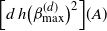$\Big[d \, h\big(\beta_\textrm{max}^{(d)}\big)^2\Big] (A)$ . This is equivalent to the original $\beta^{(d)}(t)$ process ‘reflecting’ by always proposing a positive move from 1, instead of proposing either a positive or a negative (always-rejected) move with probability $1/2$ each. We show in Section 7 that this minor modification will not change the limiting distribution of the $W_t^{(d)}$ , and thus does not affect the proof.

Thus, to first order as $\delta \searrow 0$ (i.e. up to o(1) errors), our modified process $W_t^{(d)}$ will move from $w_\textrm{max}^{(d)}$ to $\big(w_\textrm{max}^{(d)}\big) - d^{-1/2} / s_1 h\big(\beta_\textrm{max}^{(d)}\big)$ at Poisson rate $\Big[d \, h\big(\beta_\textrm{max}^{(d)}\big)^2\Big] (A)$ . Hence, setting $x=w_\textrm{max}^{(d)} = 1/s_1$ , we have

\begin{multline*} \frac{{\mathbb E}\big[f\big(W^{(d)}_{\delta}\big) \mid W^{(d)}_0=x\big] - f(x)}{{\delta}} \\ = \Big[d \, h\big(\beta_\textrm{max}^{(d)}\big)^2\Big] (A) \big[ f\big( \big(w_\textrm{max}^{(d)}\big) - d^{-1/2} / s_1 h\big(\beta_\textrm{max}^{(d)}\big) \big) - f(x) \big] + o(1) .\end{multline*}

Then, taking a Taylor series expansion around $x=w_\textrm{max}^{(d)} = 1/s_1$ ,

\begin{align*} & \frac{{\mathbb E}\Big[f\big(W^{(d)}_{\delta}\big) \mid W^{(d)}_0=x\Big] - f(x)}{{\delta}} \\[2pt] & \qquad = - \Big[d \, h\big(\beta_\textrm{max}^{(d)}\big)^2\Big] (A) \Big[ d^{-1/2} / s_1 h\big(\beta_\textrm{max}^{(d)}\big) \Big] f'\Big(w_\textrm{max}^{(d)}\Big) \\[2pt] & \qquad \quad + \tfrac{1}{2} \Big[d \, h\big(\beta_\textrm{max}^{(d)}\big)^2\Big] (A) \Big[ d^{-1/2} / s_1 h\big(\beta_\textrm{max}^{(d)}\big) \Big]^2 f''\big(w_\textrm{max}^{(d)}\big) + O(d^{-1/2}) + o(1) \\[2pt] & \qquad = - \Big[A d^{1/2} h\big(\beta_\textrm{max}^{(d)}\big) / s_1\Big] \, f'\big(w_\textrm{max}^{(d)}\big) + \tfrac{1}{2} \big[A / s_1^2\big] \, f''\big(w_\textrm{max}^{(d)}\big) + O(d^{-1/2}) + o(1) .\end{align*}

Since $f\in\mathcal{D}$ , we have $f'\big(w_\textrm{max}^{(d)}\big)=0$ , so the first term vanishes. Furthermore, it is shown in [Reference Tawn, Roberts and Rosenthal31] that, as $d\to\infty$ , $A \to 2 \, \Phi\left( {- \ell_0} / {2 \sqrt{r_1}} \right) = s_1^2$ . Hence,

\begin{equation*}\frac{{\mathbb E}\big[f\big(W^{(d)}_{\delta}\big) \mid W^{(d)}_0=x\big] - f(x)}{{\delta}} = 0 + \tfrac{1}{2} \, [1] \, f''\big(w_\textrm{max}^{(d)}\big) + O(d^{-1/2}) + o(1) ,\end{equation*}

so that

\begin{align*} \lim_{d\to\infty} G^{(d)}f\big(w_\textrm{max}^{(d)}\big) & = \lim_{d\to\infty} \, \lim_{\delta \searrow 0} \frac{{\mathbb E}\big[f\big(W^{(d)}_\delta\big) \mid W^{(d)}_0=x\big] - f(x)}{\delta} \\[3pt] & = \tfrac{1}{2} f''\big(w_\textrm{max}^{(d)}\big) = G^*\big(w_\textrm{max}^{(d)}\big) ,\end{align*}

as required.

6.3.3. Verification of (18)

To prove (18), note that if the original inverse-temperature process $\beta^{(d)}(t)$ proposes to move in time 1 from $\beta_\textrm{max}^{(d)}$ to $\beta_\textrm{max}^{(d)} - \ell\big(\beta_\textrm{max}^{(d)}\big) d^{-1/2}$ in one of the two modes (with probabilities $w_1$ and $w_2$ respectively), then by (12) the $H^{(d)}_t$ process proposes to move at rate $\Big[d \, h\big(\beta_\textrm{max}^{(d)}\big)^2\Big]$ from $1+\big[{h\big(\beta_\textrm{max}^{(d)}\big)} / {h\big(\beta_\textrm{max}^{(d)}\big)}\big] = 2$ to

\begin{align*} \pm \left[ 1 + \frac{h\big( \beta_\textrm{max}^{(d)} - \ell\big(\beta_\textrm{max}^{(d)}\big) d^{-1/2} \big) }{h\big(\beta_\textrm{max}^{(d)}\big)} \right] & = \pm \left[ 2 - \frac{\int_{\beta_\textrm{max}^{(d)}-\ell\left(\beta_\textrm{max}^{(d)}\right) d^{-1/2}}^{\beta_\textrm{max}^{(d)}} \frac{1}{\ell(u)} \, \textrm{d} u }{h\big(\beta_\textrm{max}^{(d)}\big)} \right] \\[3pt] & \approx \pm \left[ 2 - \left( \ell\big(\beta_\textrm{max}^{(d)}\big) d^{-1/2} \right) \frac{1}{\ell\big(\beta_\textrm{max}^{(d)}\big)} \right] = \pm (2-d^{-1/2}) .\end{align*}

Simultaneously, the $Z^{(d)}_t$ process proposes to move from $2-2=0$ to $\pm 2 - [\pm (2 - d^{-1/2})] = \pm d^{-1/2}$ , and the $W^{(d)}_t$ process proposes to move from 0 to either $d^{-1/2}/s_1$ or $-d^{-1/2}/s_2$ . Hence, similar to the above (but without the minor modification), with $x=0$ we have, to first order as $\delta\searrow 0$ ,

(21) \begin{align} &\frac{{\mathbb E}[f(W_{\delta}) \mid W_0=x] - f(x)}{{\delta}} = \nonumber\\[3pt] & [d \, h\big(\beta_\textrm{max}^{(d)}\big)^2] \big( w_1 \alpha_1 [f ( d^{-1/2} / s_1 ) - f(0) ] + w_2 \alpha_2 [f (\!- d^{-1/2} / s_2 ) - f(0) ] \big) + o(1) ,\end{align}

where $\alpha_i$ is the acceptance probability for the original process to accept a proposal to increase the inverse temperature from $\beta_\textrm{max}^{(d)}$ to $\beta_\textrm{max}^{(d)} - \ell\big(\beta_\textrm{max}^{(d)}\big) d^{-1/2}$ in mode i. Now, the argument in [Reference Tawn, Roberts and Rosenthal31] shows that, as $d\to\infty$ ,

\begin{equation*}\alpha_i \to 2 \, \Phi\left( \frac{- \ell_0}{{2 \sqrt{r_i}\,}} \right) = s_i^2 ,\qquad i=1,2 .\end{equation*}

Hence, taking a Taylor series expansion around $x=0$ , we obtain from (21) that

\begin{align*} & \frac{{\mathbb E}[f(W_{\delta}) \mid W_0=x] - f(x)}{{\delta}} \\[3pt] & \qquad = d \, w_1 s_1^2 (d^{-1/2} / s_1 ) f'^+(0) + \tfrac{1}{2} d \, w_1 s_1^2 (d^{-1/2} / s_1 )^2 f''^+(0) + O(d \, d^{-3/2}) + o(1) \\[3pt] & \qquad \quad - d \, w_2 s_2^2 (d^{-1/2} / s_2 ) f'^-(0) + \tfrac{1}{2} d \, w_2 s_2^2 (d^{-1/2} / s_2 )^2 f''^-(0) + O(d \, d^{-3/2}) + o(1) \\[3pt] & \qquad = d^{1/2} [ w_1 s_1 f'^+(0) - w_2 s_2 f'^-(0) ] + \tfrac{1}{2} [ w_1 f''^+(0) + w_2 f''^-(0) ] + O(d^{-1/2}) + o(1) .\end{align*}

Now, by the definition of $f\in \mathcal{D}$ , $w_1 s_1 f'^+(0) - w_2 s_2 f'^-(0) = 0$ , and $w_1 f''^+(0) + w_2 f''^-(0) = (w_1+w_2) f''(0) = f''(0)$ . Hence, we obtain finally that

\begin{equation*}\frac{{\mathbb E}[f(W_{\delta}) \, | \, W_0=x] - f(x)}{{\delta}} =\tfrac{1}{2}f''(0) + O(d^{-1/2}) + o(1) ,\end{equation*}

so that

\begin{equation*}\lim_{d\to\infty} G^{(d)}f(0) = \lim_{d\to\infty} \, \lim_{\delta \searrow 0}\frac{{\mathbb E}\big[f\big(W^{(d)}_\delta\big) \mid W^{(d)}_0=x\big] - f(x)}{\delta}= \tfrac{1}{2} f''(0)= G^*(0) .\end{equation*}

This establishes (18), and hence completes the proof of Theorem 3.

Remark 4. Because of our transformations converting $\beta^{(d)}(t)$ to $W^{(d)}_t$ , the limiting process W in Theorem 4 was skew Brownian motion on a continuous interval. It is also possible to consider diffusions directly associated with a discrete graph; see, e.g., [Reference Freidlin and Weber8].

7. Appendix: Modified processes’ occupation times

Recall that the proof of (20) in Section 6.3.2 was actually for a minor modification of the process $W_t^{(d)}$ that speeds up time by a factor of 2 whenever it is in the state $w_\textrm{max}^{(d)}$ . We now argue that this minor modification does not affect the limiting distribution. Indeed, since the modification corresponds to adjusting the rate of time, we can write the modified process as $\widehat{W}_t^{(d)}\equiv W_{\tau_d(t)}^{(d)}$ , where $\tau_d(t)$ is the time scale including the occasional speedups. Clearly, $\lim_{t \searrow 0} \tau_d(t) = 0$ . Also, it follows from Proposition 2 below that the fraction of time that the original process spends at $w_\textrm{max}^{(d)}$ converges to 0 as $d\to\infty$ . This implies that $\lim_{d\to\infty} (\tau_d(t) / t) = 1$ . Since our process $W_t^{(d)}$ is continuous, this means that $\lim_{d\to\infty} \Big|f\bigl(W_{\tau_d(t)}^{(d)}\bigr) - f\bigl(W_t^{(d)}\bigr)\Big| = 0$ . That is, the two processes have the same limiting behaviour as $d\to\infty$ . So, the diffusion limit is not affected by making our minor modification as above.

It remains to state and prove Proposition 2. We begin with a result about limiting probabilities for reflecting a simple symmetric random walk.

Figure 4.

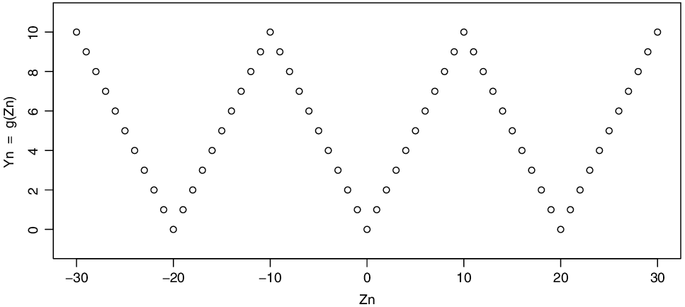
The lifting transformation function ‘g’ (when $m=10$ ).

Proof. We condition on $Y_0=y$ ; the general case then follows by taking expectation with respect to $Y_0$ . We ‘lift’ $\{Y_n\}$ to ${\mathbb Z}$ by writing $Y_n = g(Z_n)$ , where $\{Z_n\}$ is a simple symmetric random walk on all the integers ${\mathbb Z}$ , and $g(z) = \min_j |z-2jm|$ (see Figure 4). Then

\begin{multline*} {\mathbb P}_y[Y_n=0] = {\mathbb P}_y[g(Z_n)=0] = \sum_{j\in{\mathbb Z}} {\mathbb P}_y[Z_n=2jm] \\ = \sum_{j\in{\mathbb Z}} {\mathbb P}_y\Big[{\rm Binomial}(n,1/2) = \frac{n}{2} + \frac{y}{2} + jm\Big] = \sum_{j\in{\mathbb Z}} h\left(\frac{n}{2}+\frac{y}{2}+jm\right) ,\end{multline*}

where $h(k) = {\mathbb P}[{\rm Binomial}(n,1/2) = k]$ . Now, h is maximised when $k=n/2$ (or $(n\pm 1)/2$ if n is odd), and decreases monotonically on either side of that. Hence, find $j_*\in{\mathbb N}$ with $\frac{y}{2}+(j_*-1)m < 0 \le \frac{y}{2}+j_*m$ . It follows from Stirling’s approximation (see, e.g., [Reference Rosenthal27]) that to first order as $n,k,n-k\to\infty$ ,

\begin{equation*}{\mathbb P}[{\rm Binomial}(n,1/2) = k] \le \textrm{e}^{-2n[\tfrac{1}{2}-\frac{k}{n}]^2} \sqrt{1 / 2 \pi k [1-(k/n)]} ,\end{equation*}

so in particular $h\left(\frac{n}{2}+\frac{y}{2}+j_*m\right) \le \sqrt{2/\pi n} + o_n(1) \le 1/\sqrt{n}$ for all sufficiently large n, and similarly for $h\left(\frac{n}{2}+\frac{y}{2}+(j_*-1)m\right)$ . Then, by monotonicity, we have, for $j>j_*$ ,

\begin{multline*} h\bigg(\frac{n}{2}+\frac{y}{2}+jm\bigg) \le \frac{1}{m} \bigg[ h\bigg(\frac{n}{2}+\frac{y}{2}+(j-1)m+1\bigg)+h\bigg(\frac{n}{2}+\frac{y}{2}+(j-1)m+2\bigg) \\ + \cdots + h\bigg(\frac{n}{2}+\frac{y}{2}+jm\bigg) \bigg] .\end{multline*}

Hence,

\begin{equation*}\sum_{j > j_*} h\bigg(\frac{n}{2}+\frac{y}{2}+jm\bigg) \le \frac{1}{m} \bigg[ h\bigg(\frac{n}{2}+\frac{y}{2}+1\bigg)+h\bigg(\frac{n}{2}+\frac{y}{2}+2\bigg)+h\bigg(\frac{n}{2}+\frac{y}{2}+3\bigg)+\cdots \bigg] .\end{equation*}

But $\sum_k h(k) = 1$ , so by symmetry $\sum_{k>n/2} h(k) \le 1/2$ , and so

\begin{equation*}h\bigg(\frac{n}{2}+\frac{y}{2}+1\bigg)+h\bigg(\frac{n}{2}+\frac{y}{2}+2\bigg)+h\bigg(\frac{n}{2}+\frac{y}{2}+3\bigg) + \cdots \le \frac12 .\end{equation*}

Thus,

\begin{equation*}\sum_{j > j_*} h\bigg(\frac{n}{2}+\frac{y}{2}+jm\bigg) \le \frac{1}{2m} .\end{equation*}

Similarly,

\begin{equation*}\sum_{j < j_*-1} h\bigg(\frac{n}{2}+\frac{y}{2}+jm\bigg) \le \frac{1}{2m} .\end{equation*}

Therefore, for all sufficiently large n,

\begin{equation*}\sum_{j\in{\mathbb Z}} h\bigg(\frac{n}{2}+\frac{y}{2}+jm\bigg) \le(1/\sqrt{n}) + (1/\sqrt{n}) + \frac{1}{2m} + \frac{1}{2m}\ = \ (2/\sqrt{n}) + (1 / m) ,\end{equation*}

as claimed.

Proof. Let $I_i = \textbf{1}_{Y_i=0}$ be the indicator function of the event $Y_i=0$ . Then, by Proposition 1, $\lim_{n,m\to\infty} {\mathbb E}[I_n] = \lim_{n,m\to\infty} {\mathbb P}[Y_n=0] = 0$ . Hence, using the theory of Cesàro sums,

\begin{equation*}\lim_{n,m\to\infty} {\mathbb E}[N_0/n]= \lim_{n,m\to\infty} {\mathbb E}\Bigg[ \sum_{i=0}^{n-1} I_i \Bigg] / n= \lim_{n,m\to\infty} \frac{1}{n} \, \sum_{i=0}^{n-1} {\mathbb E}[I_i]= \lim_{n,m\to\infty} {\mathbb E}[I_{n}]= 0 .\end{equation*}

Hence, by Markov’s inequality, since $N_0/n \ge 0$ , for any $\epsilon>0$ we have

\begin{equation*}\lim_{n,m\to\infty} {\mathbb P}[(N_0/n) > \epsilon]\le \lim_{n,m\to\infty} {\mathbb E}[N_0/n] / \epsilon= 0 ,\end{equation*}

so that $N_0/n \to 0$ in probability, as claimed.

Proof. Let $\{J_k\}$ be the jump chain of $\{X_n\}$ , i.e. the Markov chain which copies $\{X_n\}$ except omitting immediate repetitions of the same state, and let $\{M_k\}$ count the number of repetitions. [For example, if the original chain $\{X_n\}$ began

\begin{equation*}\{X_n\} = ( a, b, b, b, a, a, c, c, c, c, d, d, a, \ldots )\end{equation*}

then the jump chain $\{J_k\}$ would begin $\{J_k\} = ( a, b, a, c, d, a, \ldots )$ and the corresponding multiplicity list $\{M_k\}$ would begin $\{M_k\} = ( 1, 3, 2, 4, 2, \ldots )$ .] Then the assumptions imply that $\{J_k\}$ has the transition probabilities of a reflecting simple symmetric random walk, as in Proposition 1 and Corollary 4.

Now, let K(n) be the smallest integer with $M_1+\cdots+M_{K(n)} \ge n$ . Given $J_k$ , the random variable $M_k$ has the Geometric $(1-p_{J_k J_k})$ distribution, so it is stochastically bounded above by the Geometric(a) distribution, from which it follows that $\lim_{n\to\infty} K(n)= \infty$ with probability 1. Let $C_s=\#\{i \,{:}\, 0 \le i \le K(n), \ J_i=s\}$ . Then Corollary 4 implies that $\lim_{n,m\to\infty} (C_0/K(n)) = 0$ . On the other hand, $N_0$ is less than or equal to a sum of $C_0$ independent Geometric $(1-p_{00})$ random variables, so ${\mathbb E}[N_0 \mid C_0] = C_0/(1-p_{00}) \le C_0/a$ , and ${\mathbb P}[N_0 > 2C_0/a \mid C_0] \to 0$ as $n\to\infty$ . Also, $M_1+\cdots+M_{K(n)-1} \le n$ , and each $M_i \ge 1$ , so $n \ge K(n)-1$ . We therefore conclude that

\begin{equation*}\lim_{n,m\to\infty} \frac{N_0}{n} \le \lim_{n,m\to\infty} \frac{2C_0/a}{K(n)-1}= ({2 / a}) \, \lim_{n,m\to\infty} \frac{C_0}{K(n)}= 0 ,\end{equation*}

as claimed.