1 Introduction
Variable-density mixing plays an important role in a wide variety of physical systems with length scales spanning many orders of magnitude, from inertial confinement fusion at the smallest (Lindl, McCrory & Campbell Reference Lindl, McCrory and Campbell1992; Amendt et al. Reference Amendt, Landen, Robey, Li and Petrasso2010), to atmospheric and oceanic flows on the global scale (Fischer Reference Fischer1979; Lee & Chu Reference Lee and Chu2003) and to mixing during stellar evolution and the explosion of supernovae (Herant et al. Reference Herant, Benz, Hix, Fryer and Colgate1994; Zingale et al. Reference Zingale, Almgren, Bell, Nonaka and Woosley2009). Variable-density effects arise any time two fluids of differing molecular weights begin to mix or when thermal or compressibility effects significantly modify the density of adjacent parcels of fluid. For density ratios close to 1, the density field can often be modelled as a passive scalar or using Boussinesq approximations, but for sufficiently high density differences these approximations no longer hold and the density gradients play an important role in the transport of fluid and the evolution of the turbulent characteristics of the flow. This becomes obvious when we write out the transport equation for momentum in a ensemble-averaged form for the case where the fluctuations in density cannot be considered negligible. For such a system
 $$\begin{eqnarray}\frac{\unicode[STIX]{x2202}}{\unicode[STIX]{x2202}t}\left(\bar{\unicode[STIX]{x1D70C}}\tilde{u} _{i}\right)+\left(\bar{\unicode[STIX]{x1D70C}}\tilde{u} _{i}\tilde{u} _{j}\right)_{,j}+\left(\bar{\unicode[STIX]{x1D70C}}\tilde{R}_{ij}\right)_{,j}=-\bar{P}_{,i}+\bar{\unicode[STIX]{x1D70F}}_{ij,j}+\bar{\unicode[STIX]{x1D70C}}g_{i},\end{eqnarray}$$
where
 $t$
is time,
 $\unicode[STIX]{x1D70C}$
is the local density,
 $u_{i}$
is velocity,
 $R_{ij}$
are the Reynolds stresses,
 $P$
is the pressure,
 $\unicode[STIX]{x1D70F}_{ij}$
is the fluid stress,
 $g_{i}$
is the acceleration due to gravity, and subscript commas followed by an index show differentiation. Here we follow the common convention of using Favre (or density-weighted) averages in addition to the typical Reynolds averaging such that a Reynolds-averaged quantity is defined by
 $\bar{x}=\left<x\right>$
where the braces indicate an ensemble-averaging operation (in this paper it will always be a time average), and the density-weighted average is computed as
 $\tilde{x}=\overline{\unicode[STIX]{x1D70C}x}/\bar{\unicode[STIX]{x1D70C}}$
. The instantaneous measures can then be decomposed into mean and fluctuating quantities as follows:
 $x=\bar{x}+x^{\prime }=\tilde{x}+x^{\prime \prime }$
. Equation (1.1) shows how the mean quantities being transported are dependent not only on the time history of the velocity fields, but also on the density. The Favre-averaged Reynolds stresses become
 $$\begin{eqnarray}\tilde{R}_{ij}=\frac{1}{\bar{\unicode[STIX]{x1D70C}}}\overline{\unicode[STIX]{x1D70C}u_{i}^{\prime \prime }u_{j}^{\prime \prime }},\end{eqnarray}$$
showing a coupling between instantaneous density and velocity fluctuations that extends to the mean turbulence quantities, in contrast to the traditional Reynolds-averaged stresses which are given by
 $\bar{R}_{ij}=\overline{u_{i}^{\prime }u_{j}^{\prime }}$
and contain only kinematic quantities. The transport of the Favre-averaged stresses is described by the equation
 $$\begin{eqnarray}\displaystyle \frac{\unicode[STIX]{x2202}(\bar{\unicode[STIX]{x1D70C}}\tilde{R}_{ij})}{\unicode[STIX]{x2202}t}+\frac{\unicode[STIX]{x2202}}{\unicode[STIX]{x2202}x_{k}}\left(\bar{\unicode[STIX]{x1D70C}}\tilde{u} _{k}\tilde{R}_{ij}\right) & = & \displaystyle a_{i}\frac{\unicode[STIX]{x2202}\bar{P}}{\unicode[STIX]{x2202}x_{j}}+a_{j}\frac{\unicode[STIX]{x2202}\bar{P}}{\unicode[STIX]{x2202}x_{i}}-\bar{\unicode[STIX]{x1D70C}}\tilde{R}_{ik}\frac{\unicode[STIX]{x2202}\tilde{u} _{j}}{\unicode[STIX]{x2202}x_{k}}-\bar{\unicode[STIX]{x1D70C}}\tilde{R}_{jk}\frac{\unicode[STIX]{x2202}\tilde{u} _{i}}{\unicode[STIX]{x2202}x_{k}}-a_{i}\frac{\unicode[STIX]{x2202}\bar{\unicode[STIX]{x1D70F}}_{jk}}{\unicode[STIX]{x2202}x_{k}}-a_{j}\frac{\unicode[STIX]{x2202}\bar{\unicode[STIX]{x1D70F}}_{ik}}{\unicode[STIX]{x2202}x_{k}}\nonumber\\ \displaystyle & & \displaystyle -\,\frac{\unicode[STIX]{x2202}}{\unicode[STIX]{x2202}x_{k}}\overline{\unicode[STIX]{x1D70C}u_{i}^{\prime \prime }u_{j}^{\prime \prime }u_{k}^{\prime \prime }}+\frac{\unicode[STIX]{x2202}}{\unicode[STIX]{x2202}x_{k}}\left(\overline{u_{i}^{\prime \prime }\unicode[STIX]{x1D70F}_{jk}^{\prime }}+\overline{u_{j}^{\prime \prime }\unicode[STIX]{x1D70F}_{ik}^{\prime }}\right)\nonumber\\ \displaystyle & & \displaystyle -\,\frac{\unicode[STIX]{x2202}}{\unicode[STIX]{x2202}x_{j}}\overline{u_{i}^{\prime \prime }P^{\prime }}-\frac{\unicode[STIX]{x2202}}{\unicode[STIX]{x2202}x_{i}}\overline{u_{j}^{\prime \prime }P^{\prime }}\nonumber\\ \displaystyle & & \displaystyle +\,\overline{P^{\prime }\frac{\unicode[STIX]{x2202}u_{i}^{\prime \prime }}{\unicode[STIX]{x2202}x_{j}}}+\overline{P^{\prime }\frac{\unicode[STIX]{x2202}u_{j}^{\prime \prime }}{\unicode[STIX]{x2202}x_{i}}}-\overline{\unicode[STIX]{x1D70F}_{jk}^{\prime }\frac{\unicode[STIX]{x2202}u_{i}^{\prime \prime }}{\unicode[STIX]{x2202}x_{k}}}-\overline{\unicode[STIX]{x1D70F}_{ik}^{\prime }\frac{\unicode[STIX]{x2202}u_{j}^{\prime \prime }}{\unicode[STIX]{x2202}x_{k}}},\end{eqnarray}$$
that is derived in Besnard et al. (Reference Besnard, Harlow, Rauenzahn and Zemach1992) and Cebeci & Smith (Reference Cebeci and Smith1974), among other sources.
 $$\begin{eqnarray}a_{i}\equiv -\overline{u_{i}^{\prime \prime }}=\overline{\unicode[STIX]{x1D70C}u_{i}^{\prime }}/\bar{\unicode[STIX]{x1D70C}}\end{eqnarray}$$
is the turbulent mass flux that is a measure of deviation caused by the variable-density nature of the flow. It is zero in the case of constant-density mixing.
As with constant-density flows, physical understanding and direct simulation of turbulent variable-density flows is difficult for any but the simplest of conditions. For typical flows of practical interest, many of the terms described in (1.3) will need to be modelled in some way (such as in Schwarzkopf et al. Reference Schwarzkopf, Livescu, Gore, Rauenzahn and Ristorcelli2011, Reference Schwarzkopf, Livescu, Baltzer, Gore and Ristorcelli2016), and devising such models (or evaluating their success) requires access to high-quality experimental datasets in canonical flows that report simultaneous measurements of the velocity and density fields. Unfortunately, such data are much more limited in availability for conditions with large density ratios than for comparable conditions with uniform density. The current study of a variable-density turbulent jet discharging into a weak coflow offers an opportunity to study the spatial evolution of a flow with significant anisotropies. We can also compare our results to many canonical studies of jets with constant or weakly perturbed densities.
Early studies of turbulent jets and plumes indicated that all jets should tend toward self-similar solutions in the far field and follow well-behaved scaling laws such that the final state is universal in both the mean and fluctuating components (Wygnanski & Fiedler Reference Wygnanski and Fiedler1969; Richards & Pitts Reference Richards and Pitts1993; Sautet & Stepowski Reference Sautet and Stepowski1995). More recent results have convincingly called into question this view, with mean quantities developing more quickly than the higher-order statistics, with the intermediate and final equilibrium states depending on the initial profile, turbulence level and other initial conditions (Boersma, Brethouwer & Nieuwstadt Reference Boersma, Brethouwer and Nieuwstadt1998; Carazzo, Kaminski & Tait Reference Carazzo, Kaminski and Tait2006; Uddin & Pollard Reference Uddin and Pollard2007). Experiments designed to quantify these differences have proven quite sensitive to the exact methods used to perform the measurements, with issues such as initial jet profiles and confinement influencing the far-field state of the flow (George Arndt & Corrsin Reference George, Arndt and Corrsin1989).
For more complicated flows, even such a simple change as the introduction of a uniform coflow or the addition density differences between the ambient and jet fluids causes significant alterations in the physics of the problem. Empirically, many of the same scaling laws seen in single-fluid jets seem to persist, but the simple forms of complete self-similarity posited for those flows cannot be analytically guaranteed for jets with variable density or in coflow. For conditions where the initial density ratio between the ambient and jet fluid is large, both the velocity and concentration field must be analysed simultaneously. The development of these jets is characterised by a momentum-dominated region near the nozzle, toward a state where buoyancy effects control the motion in the far field, with an intermediate region where both effects are important as the initial momentum is spread though mixing and energy is continually injected through density gradients and buoyant forces (Chen & Rodi Reference Chen and Rodi1980). The spatial evolution of the mixing mechanisms in jets with streamwise distance prohibits the formulation of single scaling laws that govern the entire flow evolution.
In jets with density ratios in the strongly non-Boussinesq regime, experimental information on the turbulent statistics and evolution of the jet parameters is limited. Experiments examining jets with density ratios
 $0.1<s\leqslant 1.4$
(Pitts Reference Pitts1991a
,Reference Pitts
b
; Panchapakesan & Lumley Reference Panchapakesan and Lumley1993b
; Chassaing, Harran & Joly Reference Chassaing, Harran and Joly1994; Amielh et al.
Reference Amielh, Djeridane, Anselmet and Fulachier1996; Djeridane et al.
Reference Djeridane, Amielh, Anselmet and Fulachier1996; Talbot et al.
Reference Talbot, Mazellier, Renou, Danaila and Boukhalfa2009) show how turbulent kinetic energy (t.k.e.) decays along the centreline, calculate some Reynolds-averaged quantities or provide some Favre-averaged far-field information. Effects of density fluctuations, especially in the developing, momentum-dominated region of the jet, are limited to centreline values, and most experiments do not measure the density and velocity simultaneously, limiting the conclusions that can be drawn about density fluctuation correlations.
Missing from these experiments are studies of turbulent jets with density ratios above 1.0 providing simultaneous velocity and concentration measurements along with a complete statistical description of the turbulence. A numerical parametric study of jet mixing (Harran et al.
Reference Harran, Chassaing, Joly and Chibat1996) for
 $0.14\leqslant s\leqslant 5.11$
provides some insights into the non-Boussinesq regime. That study isolates density effects using a non-gravity simulation environment and finds that density fluctuation correlations are strong in the momentum region by showing the spatial evolution of t.k.e. and turbulent mass flux.
The goal of this study is to compare the axial and radial mixing mechanisms of a jet in the Boussinesq regime, versus a non-Boussinesq jet, using turbulence statistics and complete budgets of the turbulent kinetic energy. We compare our results to available experiments and computations when possible. The experimental configurations are an air and a
 $\text{SF}_{6}$
jet discharging into a weak coflow, with measurements in the momentum region (within 30 diameters) at three different locations. Experimental measurements are made using simultaneous particle image velocimetry (PIV) and planar laser-induced fluorescence (PLIF), with 10 000 snapshots at each position to ensure good convergence of the higher-order statistics and the mean quantities. Similar methods have been used before on dye jets in water (Webster, Roberts & Ra’ad Reference Webster, Roberts and Ra’ad2001; Wang & Law Reference Wang and Law2002) and on buoyant low-speed plumes in gasses (O’Hern et al.
Reference O’Hern, Weckman, Gerhart, Tieszen and Schefer2005), but have seen limited application in high density ratio jets (Gerashchenko & Prestridge Reference Gerashchenko and Prestridge2015). This diagnostic combination provides axial and radial information that lends insights into the impact of density fluctuations on mixing.
2 Methodology
2.1 Experimental facility and test conditions
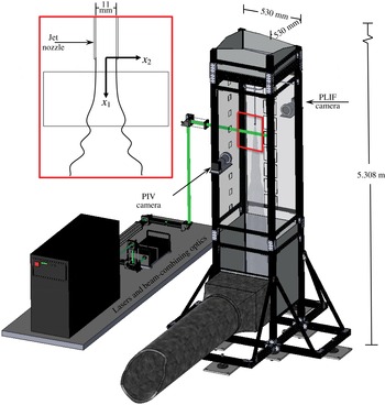
The experiments were conducted in the turbulent mixing tunnel (TMT) facility at Los Alamos National Laboratory. The TMT is a vertically oriented 0.53
 $\times$
0.53 m cross-section open circuit wind tunnel that can be driven in suction up to
 ${\sim}1.25~\text{m}~\text{s}^{-1}$
as shown in figure 1 and described by Gerashchenko & Prestridge (Reference Gerashchenko and Prestridge2015). The tunnel is instrumented for simultaneous PIV and PLIF measurements, with images acquired using a pair of TSI PowerViewPlus 11MP cameras (12 bpp,
 $4008\times 2672$
pixel maximum resolution), and illumination provided by a combination of two lasers. The first, used for PIV, is a dual head Nd:YAG laser capable of emitting up to
 $130~\text{mJ}~\text{pulse}^{-1}$
at 532 nm (Quantel Twins BSL 200). The second, used for PLIF images, is a Coherent COMPexPro XeCl excimer laser that is able to provide at least
 $250~\text{mJ}~\text{pulse}^{-1}$
of 308 nm illumination. Synchronisation is provided by a combination of a NI PXI-6602 counter timer driving the cameras and excimer laser, with a timing pulse provided to a SRS DG645 digital delay generator driving the Nd:YAG laser for better precision generating the PIV laser timing signals.
The jet flow is supplied using a
 $d_{0}=11.0~\text{mm}$
inner diameter tube (0.85 mm wall thickness) and metered using an Omega FMA2600A gas flow controller set to control the mass flow rate (in SLPM: litres per minute at standard temperature and pressure). The supply tube has a constant diameter over a length of 415 mm upstream of the exit (37.8
 $d_{0}$
), and the last bend before this run is oriented so any flow disturbance it introduces will be orthogonal to the plane of the PIV measurements. The development length for turbulent conditions at these Reynolds numbers is typically
 ${\sim}22.9d_{0}$
, so the exit flow should be fully developed, and we show that it is in § 3.2. The jet gas is bubbled through an acetone reservoir maintained at
 $19.0\,^{\circ }\text{C}$
in a recirculating bath to achieve near-saturation concentrations of acetone vapour. This acetone–gas mixture is supplied to a Laskin nozzle to generate
 ${\sim}1~\unicode[STIX]{x03BC}\text{m}$
seed particles of diethylhexyl sebacate (DEHS) for PIV (Kähler, Sammler & Kompenhans Reference Kähler, Sammler, Kompenhans, Stanislas, Westerweel and Kompenhans2004), with the concentration of particles controlled by means of a bypass valve on the particle seeder. The air flow in the tunnel was seeded for PIV using a second Laskin nozzle, supplied by compressed building air at 20 psi, and delivered to the inlet of the tunnel by means of a duct and small fan. For viewing of the flow and delivery of the laser beams, windows are installed in various locations along the length of the test section, with the unused locations blocked with solid panels. Both windows for the PIV and PLIF cameras used BK7 glass to allow transmission of near ultraviolet and visible wavelengths, while the rear window for the laser beam was of fused silica.
Rendering of turbulent mixing tunnel (TMT) and inset of jet with directional axes and sample measurement field of view.

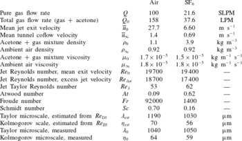
Test conditions and parameters for the two jet experiments.

The flow conditions for the two jets are given in table 1, with the non-dimensional parameters defined in (2.1). The Reynolds numbers of the two jets were approximately matched. Reported flow rates are for the dry gas before mixing with acetone; the final achieved flow rates were higher due to the added acetone. To generate the coflow in the tunnel, the blower motor was set to maximum speed for the air cases and to the minimum stable speed for the
 $\text{SF}_{6}$
cases. This meant that the shear ratio between the coflow and the jet exit velocity was not identical between the two gas mixtures, however, the Reynolds number based on excess jet velocity,
 $Re_{\unicode[STIX]{x0394}u}$
, was still very similar between the two flow conditions.
 $D$
is the diffusivity of the jet gas into the coflowing ambient air, and
 $g=9.79~\text{m}~\text{s}^{-2}$
is the estimated local gravitational acceleration.
 $$\begin{eqnarray}\displaystyle & \displaystyle Re_{0}=\frac{\unicode[STIX]{x1D70C}_{0}\cdot \overline{u}_{0}\cdot d_{0}}{\unicode[STIX]{x1D707}_{0}} & \displaystyle\end{eqnarray}$$
 $$\begin{eqnarray}\displaystyle & \displaystyle Re_{\unicode[STIX]{x0394}u}=\frac{\unicode[STIX]{x1D70C}_{0}\cdot \unicode[STIX]{x0394}\overline{u}\cdot d_{0}}{\unicode[STIX]{x1D707}_{0}} & \displaystyle\end{eqnarray}$$
 $$\begin{eqnarray}\displaystyle & \displaystyle Re_{\unicode[STIX]{x1D706}}=\frac{\unicode[STIX]{x1D70C}_{0}\bar{u}_{0}^{\prime }\unicode[STIX]{x1D706}_{0}}{\unicode[STIX]{x1D707}_{0}} & \displaystyle\end{eqnarray}$$
 $$\begin{eqnarray}\displaystyle & \displaystyle At=\frac{\unicode[STIX]{x1D70C}_{0}-\unicode[STIX]{x1D70C}_{\infty }}{\unicode[STIX]{x1D70C}_{0}+\unicode[STIX]{x1D70C}_{\infty }} & \displaystyle\end{eqnarray}$$
 $$\begin{eqnarray}\displaystyle & \displaystyle s=\unicode[STIX]{x1D70C}_{0}/\unicode[STIX]{x1D70C}_{\infty } & \displaystyle\end{eqnarray}$$
 $$\begin{eqnarray}\displaystyle & \displaystyle Fr=\frac{\unicode[STIX]{x1D70C}_{0}\bar{u}_{0}^{2}}{|\unicode[STIX]{x1D70C}_{0}-\unicode[STIX]{x1D70C}_{\infty }|gd_{0}} & \displaystyle\end{eqnarray}$$
 $$\begin{eqnarray}\displaystyle & \displaystyle Sc=\frac{\unicode[STIX]{x1D707}_{0}}{\unicode[STIX]{x1D70C}_{0}\cdot D}. & \displaystyle\end{eqnarray}$$
Taylor and Kolmogorov microscales were estimated for the centreline of the jet orifice from scaling laws (Pope Reference Pope2000) using
 $$\begin{eqnarray}\displaystyle & \displaystyle Re_{L0}=\frac{\unicode[STIX]{x1D70C}_{0}\cdot \bar{u}_{0}^{\prime }\cdot d_{0}}{\unicode[STIX]{x1D707}_{0}} & \displaystyle\end{eqnarray}$$
 $$\begin{eqnarray}\displaystyle & \displaystyle \unicode[STIX]{x1D706}_{est}=\sqrt{10}\cdot d_{0}\cdot Re_{L0}^{-1/2} & \displaystyle\end{eqnarray}$$
 $$\begin{eqnarray}\displaystyle & \displaystyle \unicode[STIX]{x1D702}_{est}=d_{0}\cdot Re_{L0}^{-3/4}, & \displaystyle\end{eqnarray}$$
 $\bar{u}_{0}^{\prime }=(\bar{R}_{ij})^{1/2}$
, using
 $\bar{R}_{ij}$
from the measured turbulent intensity at
 $x/d_{0}=0.6$
. These length scales were also calculated directly from the measured velocity and density fields on the jet centreline at
 $x/d_{0}=0.6$
using
 $$\begin{eqnarray}\displaystyle & \displaystyle \unicode[STIX]{x1D706}_{0}=\left(2\tilde{R}_{22}/\overline{(\unicode[STIX]{x2202}u_{2}^{\prime \prime }/\unicode[STIX]{x2202}x_{1})^{2}}\right)^{1/2} & \displaystyle\end{eqnarray}$$
 $$\begin{eqnarray}\displaystyle & \displaystyle \unicode[STIX]{x1D702}_{0}=\left(\bar{\unicode[STIX]{x1D708}}^{3}/\unicode[STIX]{x1D716}_{0}\right)^{1/4} & \displaystyle\end{eqnarray}$$
 $$\begin{eqnarray}\displaystyle & \displaystyle \unicode[STIX]{x1D716}_{0}=2\overline{\unicode[STIX]{x1D708}\frac{\unicode[STIX]{x2202}u_{i}^{\prime }}{\unicode[STIX]{x2202}x_{j}}\frac{\unicode[STIX]{x2202}u_{i}^{\prime }}{\unicode[STIX]{x2202}x_{j}}}. & \displaystyle\end{eqnarray}$$
Ten thousand PIV and PLIF images were captured simultaneously, at 1 Hz, at three locations downstream of the jet nozzle at
 $x_{1}/d_{0}\approx 2$
, 16 and 30 where
 $x_{1}$
is the downstream distance from the nozzle, as shown in the inset in figure 1. The length of the momentum-dominated region of the jet (Chen & Rodi Reference Chen and Rodi1980) is defined by the density ratio and the initial densimetric Froude number (2.1f
) computed with respect to centreline properties,
 $$\begin{eqnarray}X_{I}=\frac{x_{1}/d_{0}}{Fr^{1/2}s^{1/4}}.\end{eqnarray}$$
 $X_{I}=0.5$
corresponds to downstream distances of
 $x_{1}/d_{0}\approx$
158 and 27 for the air and
 $\text{SF}_{6}$
cases, respectively. The buoyancy dominated region is expected to begin near
 $X_{II}=10X_{I}$
, with an intermediate region falling in between these two extents. Thus, the measurements for both cases fall within the momentum-dominated region of the jets as defined in (2.4).
2.2 Particle image velocimetry
Images for PIV were acquired in dual exposure mode under timing and magnification conditions described in table 2. The image resolution is
 $17.94~\unicode[STIX]{x03BC}\text{m}~\text{pixel}^{-1}$
using a 200 mm macro lens, and a 532 nm notch filter between the lens and the tunnel window blocked the UV laser pulses and fluorescence signals. The acquired images used the full resolution of the sensor for a
 $71.9~\text{mm}\times 47.9~\text{mm}$
field of view (
 $6.5d_{0}\times 4.3d_{0}$
), though the region illuminated by the laser sheet was only approximately 30 mm high (
 ${\approx}3d_{0}$
). The laser sheet was focused to approximately 1.0 mm in thickness within the field of view. The time delays were optimised to capture the large dynamic range between the maximum centreline jet displacement and the outer coflow.
PIV image timing and displacement parameters.
 $\unicode[STIX]{x0394}t$
is the interframe time,
 $\unicode[STIX]{x0394}x_{max}$
refers to the average peak displacement along the jet centreline and
 $\unicode[STIX]{x0394}x_{tunnel}$
is the mean displacement in the coflow.

Velocity fields were processed using four passes of iterative image deformation with bicubic image interpolation and Gaussian smoothing between passes only, and robust phase correlation (Eckstein & Vlachos Reference Eckstein and Vlachos2009a
,Reference Eckstein and Vlachos
b
) with Gaussian windowing regions for determination of the displacements. Higher-order image interpolators were tested (
 $8\times 8$
sinc, bsplines) but the difference in the final result was small and the computational time was considerably higher. The resolution of the windows was
 $32\times 32$
pixels on the final pass (0.574 mm) with 16-pixel grid spacing (0.287 mm). Vectors failing either a velocity or correlation peak ratio test were discarded, and the remaining measurements were validated using universal outlier detection (Westerweel & Scarano Reference Westerweel and Scarano2005), with replacement by bicubic interpolation of valid vectors.
2.3 Quantitative planar laser-induced fluorescence
The field of view and magnification for the PLIF cameras was set as close as possible to the PIV images using the same 200 mm lens set-up described in § 2.2. To boost the acetone fluorescence signal on the camera sensor, the analogue gain was increased by
 $4\times$
over factory default along with a
 $4\times 4$
binning. For the
 $16d_{0}$
and
 $30d_{0}$
fields, the excimer laser was set to
 $135~\text{mJ}~\text{pulse}^{-1}$
and was used with a
 $1/2\times$
prescaling to avoid oversaturating the sensor. For the
 $2.0d_{0}$
position the laser energy was increased to
 $245~\text{mJ}~\text{pulse}^{-1}$
, the digital prescaling was adjusted to
 $1\times$
and the analogue gain was reduced by a factor of
 $1/4$
(back to the default) in an effort to boost the signal-to-noise ratio by reducing the amplification of background light. However, post-processing revealed no significant differences in sensitivity between the two conditions. A lowpass filter was placed between the tunnel window and the lens, blocking scattered light from the 532 nm laser pulses. The UV laser sheet from the excimer laser was focused and collimated to coincide with the 532 nm beam used in the PIV measurements and had a thickness in the field of view of approximately 1 mm.
Conversion of the raw imaged intensity fields to densities was performed by first calibrating the camera response for the given light sheet shape, acetone concentration and sensor performance, and then using that information to correct the experimental images (Van Cruyningen, Lozano & Hanson Reference Van Cruyningen, Lozano and Hanson1990). The steps are outlined below.
-
(i) Flat field correction. A flat field image (uniform light illuminating a flat white target) is used to normalise the spatially varying gain due to camera lens and sensor sensitivity effects.
-
(ii) Remove background light. Background images of the tunnel with the lasers firing but no jet flow are subtracted.
-
(iii) Correct for non-uniform laser light. Light sheet calibration images were acquired using a glass box large enough to fill the field of view, and the box was positioned so the first inside edge of the glass was just visible at the edge of each image with the relative positioning of the laser sheet and camera identical to the arrangement used for the matching experimental station. The box was filled with the same acetone and gas mixture that would be used during testing and was supplied continuously at the same flow rate in order to match the experimental properties of the test conditions, with the exception that the DEHS particles were excluded to avoid build-up on the walls of the calibration fixture. These images of the mixture in the glass box were then used for determining the intensity of the light sheet in the field of view. The analysis of the calibration data revealed that the beam profile of the excimer laser slowly evolved in a predictable manner based on the time the laser had been running. Using the vertical beam profile information acquired during calibration, and the known start times of the laser, a surface was fitted to the data and used to reconstruct the actual time-varying shape of the beam for any given snapshot in the flow.
-
(iv) Scale intensity from zero to one. To obtain calibration information that relates image intensity to local acetone concentration, images were acquired with jet flowing at full speed and in laminar flow to visualise the potential core, where 100 % concentration of the jet gas could be assured. Then the intensities in the image were scaled linearly from zero, no jet gas, to one, 100 % jet gas.
-
(v) Beer’s law correction. The intensity fields were then averaged in the vertical direction to yield a beam attenuation profile, and this curve was fit to an attenuation calibration function using Beer’s law, yielding an estimated acetone concentration.
-
(vi) Conversion to density. With the original concentration of acetone in the jet known, the local density was computed using the assumption that any observed decrease in the acetone concentration was due to mixing with the outer coflow. The absorption cross-section of acetone given by Thurber (Reference Thurber1999, p. 155) was used for this measurement. For datasets acquired at the
 $16d_{0}$
and
$30d_{0}$
positions, estimates of the discharge acetone concentrations were made based on measured environmental conditions and used to adjust the calibration coefficients for the peak camera intensity (in counts) corresponding to pure jet fluid illuminated by full pulse energy for the measured conditions.
-
(vii) Enforce constant volume flux. Finally, an additional small correction was applied to the final vertical profile by combining the PIV and PLIF data to ensure that the volume flux was constant along the axial direction according to the method of Sarathi et al. (Reference Sarathi, Gurka, Kopp and Sullivan2011).


Careful propagation of uncertainties in each of the steps above led to a final estimate of concentration uncertainty on an instantaneous snapshot of
 ${\sim}1{-}4\,\%$
of full scale, depending on position within the image. Many of these effects arise due to systematic uncertainty in the gain corrections, and thus are only minimally attenuated by averaging across the entire ensemble of 10 000 snapshots.
Registration of the PIV and PLIF image sets was by means of a transparent target with a dot grid placed at the jet centreline and imaged by both cameras. After conversion of the intensity fields to quantitative densities, the density fields were smoothed with a Gaussian filter to reduce the effect of camera noise, and an affine transform and bicubic interpolation were used to resample the smoothed fields to the sampling locations for the PIV images so that correlated density and velocity statistics could be computed. The radius of the smoothing kernel was chosen at
 $289~\unicode[STIX]{x03BC}\text{m}$
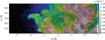
(4 PLIF pixels), to match the effective resolution of the PIV interrogation windows. A sample of a single, instantaneous image with combined PIV and PLIF velocity and density fields is shown in figure 2.
Instantaneous image of air jet density and velocity fields at
 $30d_{0}$
. The image is at full resolution, so it is best viewed digitally magnified.

3 Evolution of the mean jet structure
The current experiments were not designed to examine the jet centreline evolution in detail. However, we show in this section that mean jet properties are all consistent with previous experiments. We present the jet centreline development, initial mass and velocity profiles, and their downstream evolution at our three measurement locations for reference and use in numerical simulations.
3.1 Normalisation of mean profiles
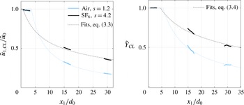
The profiles for the centreline mean velocity and mass fraction, shown in figure 3, start off very close to constant in the region of the flow nearest the pipe orifice due to the presence of an unmixed potential core and then decay asymptotically with distance as the jet spreads and mixes. Centreline measurements are normalised by the peak values measured close to the orifice, and the Favre averages are computed in a density-weighted sense. The smaller density ratio for the air jet causes this decay to happen more rapidly because mixing is more easily induced in lighter fluids with smaller momentum. This behaviour is consistent with variable-density, low-speed shear layers, where mixing layer growth is a function of the velocity and density ratios of the two layers, as observed by Brown & Roshko (Reference Brown and Roshko1974) and analytically described by Dimotakis (Reference Dimotakis1986). The faster mixing of lighter fluids versus heavy was also observed in the direct numerical simulations of Rayleigh–Taylor instability by Livescu & Ristorcelli (Reference Livescu and Ristorcelli2008), where they observed asymmetry in the mixing process.
Centreline velocity development near the jet exit is usually normalised using the effective diameter,
 $d_{eff}$
. Thring & Newby (Reference Thring and Newby1953) defined a far-field value for this quantity as
 $d_{eff\infty }=d_{0}s^{1/2}$
that gives the diameter of an equivalent jet of ambient fluid with the same momentum flux as the variable-density jet. This normalisation is implicit in the scalings outlined for the momentum-dominated region in the review of Chen & Rodi (Reference Chen and Rodi1980), and many researchers have used this form for comparing the development of jets of varying density ratios both near the orifice and in the far field (Pitts Reference Pitts1986, Reference Pitts1991a
,Reference Pitts
b
; Panchapakesan & Lumley Reference Panchapakesan and Lumley1993b
; Amielh et al.
Reference Amielh, Djeridane, Anselmet and Fulachier1996).

Variable-density jets in coflow require a definition that accounts for the development of the jet as it transitions from pure fluid exiting from the orifice with an arbitrary velocity profile to a far-field profile with density very near the ambient (Sautet & Stepowski Reference Sautet and Stepowski1995). In the case with coflow,
 $d_{eff}$
as a function of downstream distance from the jet exit becomes
 $$\begin{eqnarray}d_{eff}(x_{1})=d_{0}\sqrt{\frac{\unicode[STIX]{x1D70C}_{0}}{\unicode[STIX]{x1D70C}_{eff}(x_{1})}},\end{eqnarray}$$
where
 $$\begin{eqnarray}\unicode[STIX]{x1D70C}_{eff}(x_{1})=\frac{\displaystyle \int _{0}^{\infty }\bar{\unicode[STIX]{x1D70C}}\bar{u}_{1}(\bar{u}_{1}-\bar{u}_{\infty })\,d(r^{2})}{\displaystyle \int _{0}^{\infty }\bar{u}_{1}(\bar{u}_{1}-\bar{u}_{\infty })\,d(r^{2})}.\end{eqnarray}$$
Here
 $\unicode[STIX]{x1D70C}_{eff}$
is the mean density of the jet at a given downstream distance, weighted by the excess momentum flux, and
 $d_{eff}$
is the diameter of a jet of pure ambient fluid that would have the same induced momentum flux at that station as the variable-density jet being studied.
 $d_{eff}$
now evolves from
 $d_{0}$
near the origin to
 $d_{eff\infty }$
in the far field.
Rather than using excess velocity, Sautet & Stepowski (Reference Sautet and Stepowski1995) suggest normalising using excess momentum,
 $$\begin{eqnarray}\left(\frac{\bar{u}_{0}^{2}-\bar{u}_{0}\bar{u}_{\infty }}{\tilde{u} _{1,CL}^{2}-\bar{u}_{\infty }^{2}}\right)^{1/2}=K_{u_{CL}}\left(\frac{x_{1}-x_{u_{CL}}}{d_{eff}}\right),\end{eqnarray}$$
where the axial positions,
 $x_{1}$
, have been adjusted for a virtual origin
 $x_{u_{CL}}$
. In (3.3)
 $\tilde{u} _{1,CL}$
is the Favre-averaged centreline axial velocity. The equivalent normalisation for the mass fraction is
 $$\begin{eqnarray}\frac{1}{{\tilde{Y}}_{CL}}=K_{Y_{CL}}\left(\frac{x_{1}-x_{Y_{CL}}}{d_{eff}}\right).\end{eqnarray}$$
This scaling is applicable for
 $X_{I}\leqslant 0.5$
, the conditions of the current study.
3.2 Mean velocity and concentration development
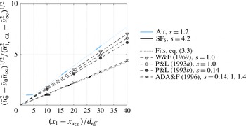
Figure 4 shows the centreline velocity decaying more slowly as the jet density ratio increases. This is in contrast with the results of Panchapakesan & Lumley (Reference Panchapakesan and Lumley1993a
,Reference Panchapakesan and Lumley
b
), who showed a slight increase and Amielh et al. (Reference Amielh, Djeridane, Anselmet and Fulachier1996), who showed saw no change, as shown in figure 4. On the other hand, the current result is in agreement with the simulations of Chassaing et al. (Reference Chassaing, Harran and Joly1994), which show decay rate decreasing with increasing density ratio, for
 $s=1.0$
and 1.43 in the intermediate region of the jet, between
 $X_{I}=0.5$
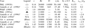
and 5.0. Furthermore, as reviewed in that work, previous experiments overall have also shown a decreasing trend for the decay rate with increasing density ratio. Table 3 shows the calculated centreline decay rates and virtual origins for the jets according to (3.3). The heavy
 $\text{SF}_{6}$
jet velocity decays less quickly than air jets from most current and previous experiments. In addition, the virtual origin seems to be decreasing with increasing density ratio, which can also be observed in the previously reported results.
Table 3 lends some insight into velocity development for the range of variable-density experiments that have been performed. The table shows the measurement regions span a range of distances across the momentum-dominated or intermediate development regions of the jets. This likely contributes to the considerable scatter between experiments by different researchers, in addition to differences in jet initial conditions (pipe flow versus top hat exit profiles) and the way the curve fits were done on the data.
Development of the centreline velocity pseudo-similarity scaling for momentum-dominated regions using the initial centreline velocity. Previously published linear fits are included for comparison, with the flow conditions described in more detail in table 3. Symbols are used for reference only.

Fitting parameters for centreline velocity development for the experiments presented in figure 4 as well as selected numerical results.

a Amielh et al. (Reference Amielh, Djeridane, Anselmet and Fulachier1996) fitted all three cases simultaneously with a single slope and different virtual origins, and report reduced centreline velocity decay rates, likely due to confinement effects at their facility.
b Chassaing et al. (Reference Chassaing, Harran and Joly1994) are fitted to simulations, but compared with experiments under the same conditions.
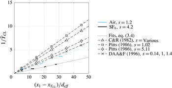
Development of the centreline mass fraction pseudo-similarity scaling in the momentum-dominated region. Previously published linear fits are included for comparison, with the flow conditions described in more detail in table 4. Symbols are used for reference only.

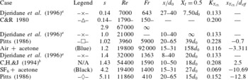
Fitting parameters for centreline mass fraction decay for the experiments presented in figure 5 as well as selected numerical results.

a Djeridane et al. (Reference Djeridane, Amielh, Anselmet and Fulachier1996) fitted all three cases simultaneously with a single slope and different virtual origins.
b Chassaing et al. (Reference Chassaing, Harran and Joly1994) are fitted to simulations, but compared with experiments under the same conditions.
Unlike decay rates of the centreline velocity, the trend of decreasing mass fraction decay rate with increasing density ratio is consistent across experiments and simulations, as shown in figure 5. The mass fraction decay we observe along the centreline agrees well with the pseudo-similarity scaling proposed by Chen & Rodi (Reference Chen and Rodi1980) for the momentum-dominated region but is slower than the decay reported by many previous researchers. A complete list of the fitted parameters is given in table 4. Most noticeable in this table is the clear effect of jet density ratio on the position of the virtual origin, as calculated using equation (3.4). This effect was observed by the Pitts (Reference Pitts1986) experiments shown in table 4 and Chassaing et al. (Reference Chassaing, Harran and Joly1994).
3.3 Jet spreading rates
Jet spreading rates, defined using velocity and concentration half-widths, vary considerably among jet types and among measurement quantities chosen. When we use axial velocity,
 $\tilde{u}$
, mean volume fraction,
 $\bar{X}$
, and Favre-averaged mass fraction,
 ${\tilde{Y}}$
, we can determine the spreading rates using
 $$\begin{eqnarray}\frac{r_{q_{1/2}}}{d_{0}}=K_{q}\frac{x_{1}-x_{q_{1/2}}}{d_{0}},\end{eqnarray}$$
where
 $q$
can be either
 $\tilde{u}$
,
 $\bar{X}$
or
 ${\tilde{Y}}$
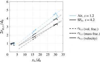
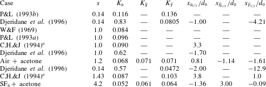
. The fits to (3.5) are shown in figure 6. The air jet spreads faster than the
 $\text{SF}_{6}$
jet, as shown by the data points and slopes (
 $K_{q}$
) in table 5. In the air jet, mass and volume fraction show equivalent spreading rates. But for the
 $\text{SF}_{6}$
jet, the mass fraction spreads 5 % faster than the volume fraction. With both jets, the trend is that using velocity to predict jet spreading rate will result in smaller spreading rates than when mass and volume fraction are used. The result is that significantly different virtual origins are calculated from these three different quantities. This result is aligned with the near-nozzle (
 $x_{1}/d_{0}=2$
) observations of the jets. More mixing is occurring early in the evolution of the
 $\text{SF}_{6}$
jet, because it shows clear spreading in both the velocity and mass fraction profiles. The volume fraction profile is narrowing, indicating that more mixing is occurring in the shear layer near the nozzle, while the
 $s=1.2$
jet spreads very little in this region.
Development of jet widths with distance calculated using (3.5) for velocity, mean volume fraction and mass fraction. The short, heavy lines are the experimental data and the light lines are the fitted functions.

Parameters for jet spreading rates (slopes),
 $K_{q}$
, and virtual origins,
 $x_{q1/2}/d_{0}$
for velocity, volume fraction and mass fraction.
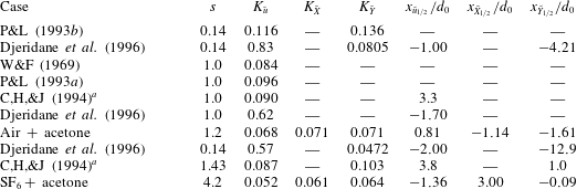
a Chassaing et al. (Reference Chassaing, Harran and Joly1994) are fitted to simulations, but compared with experiments under the same conditions.
3.4 Self-similarity of velocity and mass fraction
Although our measurements are within the momentum regions of both jets, in our downstream measurements (
 $15<x_{1}/d_{0}<31$
), we see some self-similar-like behaviour. The mean radial profiles of the axial and radial velocities (figures 7 and 8), and the mass fraction (figure 9), are shown using two different types of normalisations to demonstrate the evolution of the mean jet properties from the jet exit to the self-similar-like flow conditions.
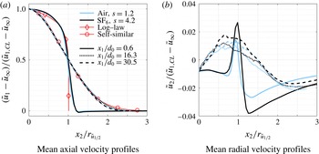
Figure 7 shows local excess axial and radial velocities at three downstream locations scaled by the centreline excess velocity, with radial coordinate by the velocity half-width,
 $r_{\tilde{u} _{1/2}}$
(the radius at which the axial speed is half the centreline). The jet exit conditions are closely matched to the log-law exit profile that would be expected for pipe flow, although slightly blunter near the jet centreline. The match to an empirical
 $1/7$
th power pipe flow profile (not shown) is also quite good, demonstrating that the mean exit flow corresponds to fully developed pipe flow. A small velocity deficit is observed outside of
 $x_{2}/d_{0}=0.6~(x_{2}/r_{\tilde{u} _{1/2}}=1.2)$
that is a remnant of the wake region created by the square ends of the jet pipe walls; this is recovered to the free stream value by
 $x_{2}/d_{0}=0.7~(x_{2}/r_{\tilde{u} _{1/2}}=1.4)$
.
Radial profiles of excess axial and radial velocity normalised by local centreline excess velocities and half-width. Expected axial asymptotic behaviour shown in red.

The scaling in figure 7(a) shows excellent collapse of the air and
 $\text{SF}_{6}$
axial velocities at each downstream position to a single profile. By
 $16d_{0}$
downstream, the excess velocity in both jets has reached a profile very similar to the Gaussian curve that is typically seen in single-fluid jets discharging into quiescent conditions. In the inner region within the half-width, the fit is nearly exact.
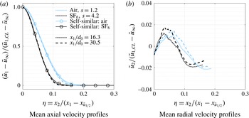
Both jets achieve self-similar conditions in the last two measurement stations (
 $x_{1}/d_{0}=16.3$
and
 $x_{1}/d_{0}$
= 31.4), as shown in figure 8(a). Using
 $$\begin{eqnarray}\unicode[STIX]{x1D702}=\frac{x_{2}}{x_{1}-x_{\tilde{u} _{1/2}}},\end{eqnarray}$$
the profiles for the air and
 $\text{SF}_{6}$
jets collapse neatly onto the Gaussian profiles
 $$\begin{eqnarray}\frac{\tilde{u} _{1}-\bar{u}_{\infty }}{\tilde{u} _{1,CL}-\bar{u}_{\infty }}=\exp \left(-A\unicode[STIX]{x1D702}^{2}\right),\end{eqnarray}$$
where the width coefficient
 $A$
is defined by the velocity half-width spreading rate and the expression (Chen & Rodi Reference Chen and Rodi1980)
 $$\begin{eqnarray}A=\frac{\ln 2}{\left(K_{\tilde{u} }\right)^{2}}.\end{eqnarray}$$
The spreading rate is larger at all times for the air jet than for the
 $\text{SF}_{6}$
, indicating faster development of the less dense jet. As mentioned previously, this effect is also observed in shear layers (Soteriou & Ghoniem Reference Soteriou and Ghoniem1995) and Rayleigh–Taylor unstable flows (Livescu & Ristorcelli Reference Livescu and Ristorcelli2008). Figure 8(a) shows that both variable-density jets are tending toward a self-similar state in the momentum-dominated region of their development, though not the same state.
Profiles of normalised axial and radial velocity using radial similarity variable (3.6).

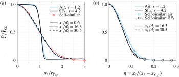
Radial profiles of mass fraction (a) normalised by local centreline value and half-width and (b) with respect to self-similarity coordinates. Expected asymptotic behaviour is shown in red.

The profiles for mass fraction, shown in figure 9(a), are very nearly top hat in profile. In the downstream locations, the jet mass fraction has begun to assume a nearly Gaussian profile for both jets, just as the velocity profile does. As with the velocity profiles, the jet half-width and centreline mass fraction do an excellent job of collapsing both the near-jet and downstream profiles (figure 9 a). Using self-similarity variables based on mass fraction also yields excellent collapse of downstream concentration profiles (figure 9 b), just as it did for the velocity profiles, although the self-similar states in the momentum region are not the same for the two jets.
4 Variable-density effects on turbulent statistics
There are two main ways that density fluctuation effects are handled in turbulence modelling. If one starts with unweighted averaging, the conservation equations for variable-density flows lead to the appearance of new terms that reflect the correlation of the density fluctuations with the other flow variables such as velocity or kinetic energy, e.g. Chassaing et al. (Reference Chassaing, Antonia, Anselmet, Joly and Sarkar2002). Analysis of these new terms must be handled separately from the terms appearing in the single-fluid case, but this approach has an advantage because the velocity fluctuation and Reynolds stresses maintain the same kinematic meanings as they do for constant-density flows. So, any models previously developed for a single-density flow should be directly applicable to variable-density flow, with the addition of the new density correlation terms.
The second approach uses density-weighted averages, such as Favre averaging, to develop forms of the governing equations that are much closer in structure to traditional single-density equations, with many of the new variable-density effects embedded in the new Favre-averaged variables. This has the benefit that mathematically, many of the same analysis tools and closure schemes developed for single-fluid equations can be directly applied to the new density-weighted forms without the need for explicit modelling of the variable-density correlation terms. The drawback is that it is not always clear whether physically these models should apply, since the Favre-averaged variables do not share the same kinematic meaning as the original Reynolds-averaged quantities.
The second approach has the advantage of converting the simplified transport equations for mean velocity in the single-fluid case (which is not a conserved quantity), into transport equations for momentum (which is, since
 $\bar{\unicode[STIX]{x1D70C}}\tilde{u} _{i}=\overline{\unicode[STIX]{x1D70C}u_{i}}$
is the time-averaged momentum). Consequently, the analysis and closures made for single-fluid flows are just special cases of more general variable-density approaches, and empirically these methods have shown great success in simulating variable-density flows over a wide range of conditions (Besnard et al.
Reference Besnard, Harlow, Rauenzahn and Zemach1992; Schwarzkopf et al.
Reference Schwarzkopf, Livescu, Gore, Rauenzahn and Ristorcelli2011, Reference Schwarzkopf, Livescu, Baltzer, Gore and Ristorcelli2016).
We will examine spatial variations in turbulence intensities between the two jets and calculate Reynolds- and Favre-averaged turbulence quantities to understand the effects of density on the mixing and gain insight into modelling these quantities.
The density-weighted forms of Reynolds stresses are related to the traditional ensemble averages by the relationship
 $$\begin{eqnarray}\displaystyle \tilde{R}_{ij}\equiv \overline{u_{i}^{\prime \prime }u_{j}^{\prime \prime }} & = & \displaystyle \overline{u_{i}^{\prime }u_{j}^{\prime }}-(\overline{\unicode[STIX]{x1D70C}u_{i}^{\prime }}/\bar{\unicode[STIX]{x1D70C}})(\overline{\unicode[STIX]{x1D70C}u_{j}^{\prime }}/\bar{\unicode[STIX]{x1D70C}})+\overline{\unicode[STIX]{x1D70C}^{\prime }u_{i}^{\prime }u_{j}^{\prime }}/\bar{\unicode[STIX]{x1D70C}}\nonumber\\ \displaystyle & = & \displaystyle \bar{R}_{ij}-a_{i}a_{j}+\overline{\unicode[STIX]{x1D70C}^{\prime }u_{i}^{\prime }u_{j}^{\prime }}/\bar{\unicode[STIX]{x1D70C}}.\end{eqnarray}$$
Recall that
 $a_{i}$
are the turbulent mass fluxes (1.4), which are zero in the case of constant-density flows. For the turbulence intensities and t.k.e. the term
 $a_{i}a_{i}$
will be positive for variable-density mixing and acts to reduce the magnitude of the Favre-averaged Reynolds stresses as opposed to the Reynolds-averaged quantities. The final term in the relation may be positive or negative, but since it is a triple correlation and is scaled relative to the other two terms by a density fluctuation divided by the mean density, it might be expected to be smaller than the others. However, as will be seen in the next section it is not necessarily negligible. Together, the second and third terms make up the localised variable-density effects on the calculation of Reynolds stresses.
4.1 Radial profiles of Reynolds stresses
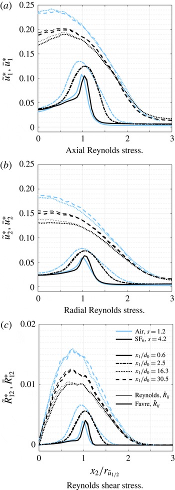
To explore the magnitude and distribution of these effects, radial profiles of Reynolds stress tensor components are plotted in both Reynolds- and Favre-averaged forms in figure 10. The mean magnitude of the fluctuating axial and radial components of velocity are plotted in figure 10 versus the downstream distance, normalised by the excess centreline momentum according to
 $$\begin{eqnarray}\bar{u}_{1}^{\ast }=\left(\frac{\bar{R}_{11}}{\bar{u}_{1,CL}^{2}-\bar{u}_{\infty }^{2}}\right)^{1/2},\quad \bar{u}_{2}^{\ast }=\left(\frac{\bar{R}_{22}}{\bar{u}_{1,CL}^{2}-\bar{u}_{\infty }^{2}}\right)^{1/2}\end{eqnarray}$$
for the Reynolds-averaged r.m.s. fluctuations and
 $$\begin{eqnarray}\tilde{u} _{1}^{\ast }=\left(\frac{\widetilde{R}_{11}}{\widetilde{u}_{1,CL}^{2}-\bar{u}_{\infty }^{2}}\right)^{1/2},\quad \tilde{u} _{2}^{\ast }=\left(\frac{\widetilde{R}_{22}}{\widetilde{u}_{1,CL}^{2}-\bar{u}_{\infty }^{2}}\right)^{1/2}\end{eqnarray}$$
for the Favre-averaged root mean square (r.m.s) fluctuations. The shear stress component is also normalised by the excess centreline momentum:
 $$\begin{eqnarray}\bar{R}_{12}^{\ast }=\frac{\bar{R}_{12}}{\bar{u}_{1,CL}^{2}-\bar{u}_{\infty }^{2}},\quad \widetilde{R}_{12}^{\ast }=\frac{\widetilde{R}_{12}}{\widetilde{u}_{1,CL}^{2}-\bar{u}_{\infty }^{2}}.\end{eqnarray}$$
This normalisation follows the functional form for the decay of the centreline velocity (3.3) suggested by Sautet & Stepowski (Reference Sautet and Stepowski1995) and yields a better collapse of the downstream profiles. It does, however, lead to smaller normalised turbulence intensities than the normalisation by
 $\bar{u}_{1,CL}-\bar{u}_{\infty }$
used by Amielh et al. (Reference Amielh, Djeridane, Anselmet and Fulachier1996), among others. When discussing results reported by Amielh et al. (Reference Amielh, Djeridane, Anselmet and Fulachier1996), we adjust their values to match (4.2).
Radial profiles of Reynolds stresses. Jet material is denoted as (blue) for air; and (black) for
 $\text{SF}_{6}$
; downstream location is given by ——,
 $x_{1}/d_{0}=0.6$
; – - – - –,
 $x_{1}/d_{0}=2.5$
;
 $\cdots \cdots \,$
,
 $x_{1}/d_{0}=16.3$
; – – –,
 $x_{1}/d_{0}=31.4$
; with (heavy lines) for Favre averages; and (light lines) for Reynolds averages.

Figure 10 shows the radial profiles of the Reynolds stresses at four different axial locations. At the upstream locations, any differences between Favre and Reynolds averaging is slight, and the curves lay on top of each other; the same is true for the air jet results downstream (
 $x_{1}=16.3d_{0}$
and
 $30.5d_{0}$
) but not the
 $\text{SF}_{6}$
. Additionally, several variable-density effects are observable in comparisons of the central portion of the two jet flows, within about
 $x_{2}/r_{\tilde{u} _{1/2}}<2$
. For the two axial locations near the jet exit, the shear is high, and we expect the flow to behave like a variable-density shear layer. Two-dimensional shear layers mix asymmetrically towards the lighter side of the layer, and the mixing entrainment is proportional to
 $s^{1/2}$
(Brown & Roshko Reference Brown and Roshko1974; Dimotakis Reference Dimotakis1986) and governed by large-scale coherent structures. In the jet shear layer, the magnitude of the normal stress components has a strong peak, shifted slightly radially outward for the heavy jet. At
 $2.5d_{0}$
, the shear layer has spread considerably and has begun to disturb the potential core while the magnitude of the fluctuations has slightly increased, due to localised production tied the large vortices characteristic of shear layer mixing. The shear layer effects are gone by
 $16d_{0}$
, where the profiles for both air and
 $\text{SF}_{6}$
have assumed very nearly the shapes expected for single-density free jets. At the downstream locations, the magnitudes of the Reynolds stresses have diverged, with peak values of air 20–30 % larger than those of
 $\text{SF}_{6}$
.
This difference in peak normal stress locations is also present in the data of Panchapakesan & Lumley (Reference Panchapakesan and Lumley1993a
,Reference Panchapakesan and Lumley
b
) and Amielh et al. (Reference Amielh, Djeridane, Anselmet and Fulachier1996), although neither set of authors discussed it. Panchapakesan & Lumley did not provide results near the nozzle, but showed for the axial fluctuation a peak near
 $0.4r_{\tilde{u} _{1/2}}$
in the self-similar region of the air jet, and a peak near the centreline for helium. For Amielh et al., in the upstream shear layer there were no clear shifts in the peak for the axial fluctuations at
 $0.2d_{0}$
, but a shift is present in the radial component (0.7, 1.0 and
 $1.1r_{\tilde{u} _{1/2}}$
for He, air and
 $\text{CO}_{2}$
), and for the axial component at
 $20d_{0}$
(
 ${\approx}0.4,0.5$
and
 $0.6r_{\tilde{u} _{1/2}}$
). There may also be a similar effect present in the axial fluctuations at
 $2.0d_{0}$
, but it is more difficult to compare due to the very rapid development of the helium jet. Taking the results of these previous studies together with the present, the data seem to suggest a consistent skewing of the location of peak turbulent stresses outward for jets with density ratios
 $s>1$
, and inward for jets with
 $s<1$
. This is probably reflective of the difference in momentum transfer between a dense jet in lighter surroundings versus a light jet in a denser medium; the less dense material will be more easily accelerated and thus accumulate larger fluctuations more easily, skewing the profiles toward the direction of less mass.
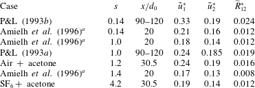
Peak Reynolds stresses for various jet experiments.
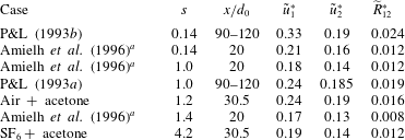
a
Amielh et al. (Reference Amielh, Djeridane, Anselmet and Fulachier1996) are rescaled using (4.2) and (4.4), and were reported as
 $\bar{R}_{ij}$
.
Table 6 shows peak Reynolds stresses from jet experiments ranging from
 $0.14\leqslant s\leqslant 4.2$
. Just as in our experiments, the trend for lower turbulence fluctuations in higher density ratio jets is seen in both the results of Panchapakesan & Lumley (Reference Panchapakesan and Lumley1993a
,Reference Panchapakesan and Lumley
b
) for free helium and air jets and in Amielh et al. (Reference Amielh, Djeridane, Anselmet and Fulachier1996) work with helium, air and CO
 $_{2}$
. Our absolute values of peak fluctuations agree well with the air jet of Panchapakesan and Lumley. The overall trend of decreasing fluctuations with increasing jet density agrees with the simulations of Chassaing et al. (Reference Chassaing, Harran and Joly1994) and Harran et al. (Reference Harran, Chassaing, Joly and Chibat1996).
Shear stress profiles have odd symmetry, as expected with values very near zero on the centreline. In the upstream region, they show a nearly linear profile within the potential core, increasing sharply to a narrow peak in the shear region that spreads with distance to overtake the whole jet downstream. Due to the anti-symmetry of the profiles, the peak is clearly off centre in the developed region (
 $30d_{0}$
); near
 $0.7r_{\tilde{u} _{1/2}}$
for the air jet and 0.8 for the
 $\text{SF}_{6}$
.
Also included in figure 10 are the Favre- and Reynolds-averaged fluctuations at the downstream locations (thick versus thin lines). For the air jet, the values are coincident, but for the
 $\text{SF}_{6}$
jet, we see the radial extent of the reduction in
 $R_{ij}$
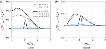
due to the variable-density conditions. This effect is caused by the variable-density terms in (4.1). We quantify the effect of the turbulent mass fluxes in figure 11, where the axial and radial turbulent mass fluxes,
 $a_{1}$
and
 $a_{2}$
are shown at the jet exit and downstream locations. The magnitude of the mass fluxes in air are always low, increasing from the jet exit and then decreasing to the furthest measurement station. These small, non-zero values are due to the air jet density ratio of
 $s=1.2$
. For the heavy jet, the mass fluxes are very high and localised at the nozzle exit in the shear layer region, spreading and increasing at the
 $x_{1}/d_{0}=16.3$
location, then decreasing but still remaining many times larger than the air values.
Turbulent mass fluxes, defined in (1.4).

The relationship between turbulent mass flux and density gradients is illustrated in Balakumar et al. (Reference Balakumar, Orlicz, Ristorcelli, Balasubramanian, Prestridge and Tomkins2012) for shock-driven Richtmyer–Meshkov mixing, where they found similar effects of turbulent mass flux on the Reynolds stresses in a reshocked heavy gas curtain (
 $s=4$
). The difference in magnitude of the turbulent mass fluxes is also observed in the calculations of Harran et al. (Reference Harran, Chassaing, Joly and Chibat1996). Our experiments and their simulations show that the peaks in
 $a_{1}$
for
 $s=4.2$
are approximately
 $7\times$
larger than those for
 $s=1.2$
, as shown in figure 11(a). We observe this same ratio between peaks for
 $a_{2}$
, as seen in figure 11(b). The shapes of the radial profiles for
 $a_{2}$
are similar to Harran et al. (Reference Harran, Chassaing, Joly and Chibat1996) figure 16, showing the peak moving inward with increasing downstream position. The importance of the turbulent mass flux in modelling and understanding variable-density mixing is also described in the direct numerical simulations of Rayleigh–Taylor instabilities by Livescu & Ristorcelli (Reference Livescu and Ristorcelli2007).
In figure 11(b), the radial turbulent mass flux,
 $a_{2}$
, goes to zero on the centreline, while the difference between
 $\bar{R}_{22}$
and
 $\tilde{R}_{22}$
does not vanish. Therefore, the triple correlation term
 $\overline{\unicode[STIX]{x1D70C}^{\prime }u_{2}^{\prime }u_{2}^{\prime }}/\bar{\unicode[STIX]{x1D70C}}$
in (4.1) is not negligible there, and must be negative and of similar magnitude to the off axis
 $a_{2}a_{2}$
. We can use
 $\overline{\unicode[STIX]{x1D70C}^{\prime }u_{2}^{\prime }u_{2}^{\prime }}$
to draw some inferences about one possible description of the instantaneous mixing conditions that could give rise to this behaviour. We expect that inward fluctuations of radial velocity (
 $u_{2}^{\prime }<0$
) should be associated with decreases of local density (
 $\unicode[STIX]{x1D70C}^{\prime }<0$
) as more dilute fluid is brought inward, and
 $\unicode[STIX]{x1D70C}^{\prime }u_{2}^{\prime }u_{2}^{\prime }<0$
for such events. Similarly, for positive velocity fluctuations (
 $u_{2}^{\prime }>0$
) less-mixed fluid is usually being transported outward (
 $\unicode[STIX]{x1D70C}^{\prime }>0$
,
 $\unicode[STIX]{x1D70C}^{\prime }u_{2}^{\prime }u_{2}^{\prime }>0$
). For the net correlation to be negative, on balance the fluid being swept inward must be more pure than the denser fluid being returned outward. The fluid being brought inward by vortical motion during an entrainment event tends to be relatively pure outer fluid that begins to mix with the surrounding jet, while the material being transported outward will tend to already be dilute. At
 $x_{2}=0$
, of course, any motions that penetrate the jet centreline will tend to be associated with less dense than average material, and thus
 $\unicode[STIX]{x1D70C}^{\prime }u_{2}^{\prime }u_{2}^{\prime }<0$
for both
 $u_{2}^{\prime }<0$
and
 $u_{2}^{\prime }>0$
. This results in the net contribution of this term being negative near the centre of the jet, reinforcing the decrease of
 $\tilde{R}_{ii}$
versus
 $\bar{R}_{ii}$
caused by the
 $a_{i}a_{i}$
term.
Development with downstream distance of centreline turbulence intensities.

4.2 Evolution of turbulent kinetic energy with axial distance
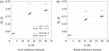
The current facility is not optimal for examining the full axial evolution of the jet due to optical access limitations. The access in the tunnel is currently under improvement, but for now we focus on trends that we see in the Reynolds stresses as we move downstream. The turbulent normal stresses are shown in figure 12 versus downstream distance, with the fluctuation magnitudes normalised according to equations (4.2) and (4.3). As before, both Favre- and Reynolds-averaged fluctuations are shown, and differences are only present for the two downstream locations in the
 $\text{SF}_{6}$
jet.
Turbulence intensities for both jets were not isotropic exiting the pipe, with axial fluctuations near 3.5 % and radial at 2.3 %, consistent with previous experimental and numerical reports for fully developed turbulent pipe flow (see, for instance, Laufer Reference Laufer1952, Wu & Moin Reference Wu and Moin2008). For both jets, the ratio of axial to radial fluctuations downstream is approximately 1.25, consistent with ranges from 0.23–0.28 axially and 0.15–0.22 radially that are reported in the literature for air. The magnitude of the fluctuations rises more quickly for the air jet plateauing by
 $30d_{0}$
near values of 0.235 and 0.19 in the axial and radial directions, regardless of which averaging is used. A similar structure is seen with the
 $\text{SF}_{6}$
jet, though the intensities may not have yet reached an asymptotic value by the final measurement location, and the magnitudes are lower, reaching only approximately 0.19 and 0.15. Our new results in the strongly non-Boussinesq regime show that an
 $s=4.2$
jet is trending toward lower asymptotic turbulence fluctuation levels compared to a jet with a density ratio of
 $s=1.2$
.
The air jet has higher turbulence intensities in figure 12 because it develops very quickly, causing the centreline velocity to drop faster than that of the
 $\text{SF}_{6}$
jet. The centreline excess normalisation used in (4.2) and (4.3) causes the air jet turbulence intensities to be larger than the
 $\text{SF}_{6}$
jet. We will separate this effect from the density fluctuation effect in a later section. The difference between Favre and Reynolds averaging is noticeable in the
 $\text{SF}_{6}$
jet, with an approximate 3–5 % decrease in magnitude for mass-weighted values due to variable-density effects at both
 $16d_{0}$
and
 $30d_{0}$
locations, but not in the region close to the nozzle. While not large, the difference is consistent, and the effect of the discrepancy on the mean flow will be cumulative with distance.
These results compare well to the experiments of Amielh et al. (Reference Amielh, Djeridane, Anselmet and Fulachier1996) who examined jets issuing from a fully developed pipe in momentum-matched flows (rather than Reynolds number) of He, air and
 $\text{CO}_{2}$
(
 $s=0.14,1.0,1.4$
), and saw that using the normalisation
 $\bar{u}_{1,CL}{-}\bar{u}_{\infty }$
all gasses reached a plateau for axial fluctuations of approximately 0.27 by 40
 $d_{0}$
, with or without coflow. This value was reached very quickly for the lighter helium flow (
 ${\sim}5d_{0}$
), but further downstream for the air and
 $\text{CO}_{2}$
jets
 $({>}30d_{0})$
. When adjusted for the normalisations in (4.2) the trends in their data become more similar to the present investigation. The new correction causes the turbulence levels to plateau much earlier, by approximately
 $16d_{0}$
as is seen in the present experiments. Additionally, with this normalisation the density effect on the turbulent fluctuations appear in the data of Amielh et al. as well, with the asymptotic states for the axial fluctuations becoming approximately 0.23, 0.18 and 0.17 for helium, air and
 $\text{CO}_{2}$
respectively, and 0.17, 0.15 and 0.14 for the radial fluctuations. The rescaled values for air are slightly lower than those measured here, but still within the lower end of the range typically reported, and show the same trend of lower turbulent fluctuations for denser jets.
The turbulent kinetic energy,
 $\tilde{k}$
, has also been calculated in density-weighted form from the trace of the Favre-averaged Reynolds stress tensor according to the relation
 $$\begin{eqnarray}\tilde{k}=\tilde{R}_{ii}=\tilde{R}_{11}+\tilde{R}_{22}+\tilde{R}_{33}\approx \tilde{R}_{11}+2\tilde{R}_{22}.\end{eqnarray}$$
Since
 $u_{3}$
(in the azimuthal direction) was not measured in this study,
 $\tilde{R}_{33}$
was approximated by
 $\tilde{R}_{22}$
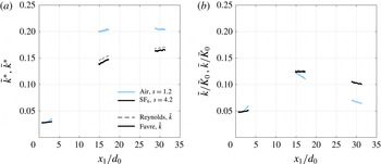
, which should be true identically in the case of radial symmetry along the jet centreline. The same form was used for calculation of Reynolds-averaged t.k.e. The results are plotted in figure 13 with two different scaling methods. The first is with the scaling of
 $(2/3\tilde{k})^{1/2}$
or
 $(2/3\bar{k})^{1/2}$
to match the magnitudes of the turbulence intensities for Favre or Reynolds averaging, respectively, and normalised again by the excess momentum using the relations
 $$\begin{eqnarray}\bar{k}^{\ast }=\left(\frac{2/3\hspace{1.4457pt}\bar{k}}{\bar{u}_{1,CL}^{2}-\bar{u}_{\infty }^{2}}\right)^{1/2},\quad \tilde{k}^{\ast }=\left(\frac{2/3\hspace{1.4457pt}\tilde{k}}{\widetilde{u}_{1,CL}^{2}-\bar{u}_{\infty }^{2}}\right)^{1/2}.\end{eqnarray}$$
The second scaling in figure 13(b) uses the initial kinetic energy of the mean flow, either
 $\bar{K}_{0}$
or
 $\tilde{K}_{0}$
.
Development with downstream distance of turbulent kinetic energy along the centreline, (a) using the scaling of (4.6) and (b) scaled with the initial kinetic energy of the mean flow.

Trends in t.k.e. are similar to those observed in the component fluctuations, with the turbulent kinetic energy for the air jet appearing to asymptote by
 $30d_{0}$
to a value just above 0.20, and the
 $\text{SF}_{6}$
jet beginning to approach a final value near 0.16. As expected in an
 $s=1.2$
jet, this is close to the asymptotic value near 0.23 seen by Amielh et al. (Reference Amielh, Djeridane, Anselmet and Fulachier1996) for a slightly smaller density ratio of
 $s=1$
, and the direction of the deviation is consistent with the observed effect of increasing density ratio, though when renormalised using (4.2) the values drop to approximately 0.21, 0.15 and 0.14 for helium, air and
 $\text{SF}_{6}$
, lower than the current results. As before, values from Amielh et al. (Reference Amielh, Djeridane, Anselmet and Fulachier1996) have been renormalised to match the present scaling.
The variable-density effects that lower both the peak and asymptotic values of t.k.e. along the jet centreline were studied parametrically in the numerical simulations of Harran et al. (Reference Harran, Chassaing, Joly and Chibat1996), where they observed trends similar to figure 8. The asymptotic values of t.k.e. (
 ${\approx}0.15$
for air, and slightly lower for
 $s=5.11$
) were mostly reached at
 $x_{1}/d_{0}>300$
, which is well outside the measurements of these experiments.
Although such qualitative descriptions of the jet evolution are useful for understanding the net changes in the distribution of turbulent kinetic energy with distance and how they are affected by different jet density ratios, for a more quantitative description we need to examine the full budget equations. These are derived and discussed in the following section.
5 Turbulence budgets
5.1 Turbulent kinetic energy transport equations
To gain some insight into the mechanisms driving the variable-density effects we have observed, we examine the budgets of t.k.e. These were derived by taking one half of the trace of Favre-averaged Reynolds stress transport equations shown in (1.3). Under the assumption of statistically stationary flow, the time derivative terms were dropped. This yielded the following budget equations:
 $$\begin{eqnarray}\displaystyle & \displaystyle 0=C^{\tilde{k}}+P^{\tilde{k}}+M^{\tilde{k}}+T^{\tilde{k}}+\unicode[STIX]{x1D6F7}^{\tilde{k}}+\unicode[STIX]{x1D716}^{\tilde{k}} & \displaystyle\end{eqnarray}$$
 $$\begin{eqnarray}\displaystyle & \displaystyle C^{\tilde{k}}=-\frac{\unicode[STIX]{x2202}}{\unicode[STIX]{x2202}x_{n}}(\tilde{u} _{n}\overline{\unicode[STIX]{x1D70C}}\tilde{k})\quad \text{(advection)} & \displaystyle\end{eqnarray}$$
 $$\begin{eqnarray}\displaystyle & \displaystyle P^{\tilde{k}}=-\overline{\unicode[STIX]{x1D70C}}\tilde{R}_{ij}\frac{\unicode[STIX]{x2202}\tilde{u} _{i}}{\unicode[STIX]{x2202}x_{j}}+a_{i}\frac{\unicode[STIX]{x2202}\overline{P}}{\unicode[STIX]{x2202}x_{i}}\quad \text{(production)} & \displaystyle\end{eqnarray}$$
 $$\begin{eqnarray}\displaystyle & \displaystyle M^{\tilde{k}}=-a_{i}\frac{\unicode[STIX]{x2202}\bar{\unicode[STIX]{x1D70F}}_{ij}}{\unicode[STIX]{x2202}x_{j}}\quad \text{(molecular shear)} & \displaystyle\end{eqnarray}$$
 $$\begin{eqnarray}\displaystyle & \displaystyle T^{\tilde{k}}=-\frac{1}{2}\frac{\unicode[STIX]{x2202}}{\unicode[STIX]{x2202}x_{j}}\tilde{R}_{jii}+\frac{\unicode[STIX]{x2202}}{\unicode[STIX]{x2202}x_{j}}\overline{u_{i}^{\prime \prime }\unicode[STIX]{x1D70F}_{ji}^{\prime }}-\frac{\unicode[STIX]{x2202}}{\unicode[STIX]{x2202}x_{i}}\overline{u_{i}^{\prime \prime }P^{\prime }}\quad \text{(transport)} & \displaystyle\end{eqnarray}$$
 $$\begin{eqnarray}\displaystyle & \displaystyle \unicode[STIX]{x1D6F7}^{\tilde{k}}=\overline{P^{\prime }\frac{\unicode[STIX]{x2202}u_{i}^{\prime \prime }}{\unicode[STIX]{x2202}x_{i}}}\quad \text{(pressure strain)} & \displaystyle\end{eqnarray}$$
 $$\begin{eqnarray}\displaystyle & \displaystyle \unicode[STIX]{x1D716}^{\tilde{k}}=-\overline{\frac{\unicode[STIX]{x2202}u_{i}^{\prime \prime }}{\unicode[STIX]{x2202}x_{j}}\unicode[STIX]{x1D70F}_{ji}^{\prime }}\quad \text{(dissipation)} & \displaystyle\end{eqnarray}$$
The production term (
 $P^{\tilde{k}}$
) has two parts, the first equal to the classical effect of the Reynolds stresses acting on the straining of fluctuating part, and the second a variable-density effect where the turbulent mass flux interacts with the mean pressure strain. In the case of constant-density flow, this second term vanishes. Although the molecular shearing effects (
 $M^{\tilde{k}}$
) could be calculated from the present data, trial computations showed it was typically at least 3–4 orders of magnitude smaller than the other terms, and therefore we have omitted it from the analysis. The transport term is divided into a turbulent flux part (
 $D^{\tilde{k}}$
, first part on the right-hand side) consisting of a triple correlation of velocity with the local density,
 $\tilde{R}_{jii}=\overline{\unicode[STIX]{x1D70C}u_{j}^{\prime \prime }u_{i}^{\prime \prime }u_{i}^{\prime \prime }}$
, and fluctuating velocity–stress and fluctuating velocity–pressure correlations (the second term is flux due to fluctuating stress; the third flux from pressure fluctuations,
 $\unicode[STIX]{x1D6F1}^{\tilde{k}}$
). Many previous authors, including Panchapakesan & Lumley (Reference Panchapakesan and Lumley1993a
,Reference Panchapakesan and Lumley
b
), omitted the stress flux terms under the assumption that they are negligible. This assumption, that
 $T^{\tilde{k}}=D^{\tilde{k}}+\unicode[STIX]{x1D6F1}^{\tilde{k}}$
was assumed to be true here but was not verified. The pressure strain (
 $\unicode[STIX]{x1D6F7}^{\tilde{k}}$
) can be neglected, since for subsonic turbulence the divergence of the density-weighted fluctuations should be very near zero.
Recasting the remaining terms in cylindrical coordinates (to take advantage of symmetries in the flow) and assuming that there is no swirl (gradients of mean quantities in the azimuthal direction are 0), we obtain the following simplified expressions:
 $$\begin{eqnarray}\displaystyle C^{\tilde{k}} & = & \displaystyle -\!\left[\frac{1}{r}\frac{\unicode[STIX]{x2202}}{\unicode[STIX]{x2202}r}(r\overline{\unicode[STIX]{x1D70C}}\tilde{k}\tilde{u} _{r})+\frac{\unicode[STIX]{x2202}}{\unicode[STIX]{x2202}z}(\overline{\unicode[STIX]{x1D70C}}\tilde{k}\tilde{u} _{z})\right]\quad \text{(advection)}\end{eqnarray}$$
 $$\begin{eqnarray}\displaystyle P^{\tilde{k}} & = & \displaystyle -\overline{\unicode[STIX]{x1D70C}}\bigg[\frac{\unicode[STIX]{x2202}\tilde{u} _{r}}{\unicode[STIX]{x2202}r}\tilde{R}_{rr}+\bigg(\frac{\unicode[STIX]{x2202}\tilde{u} _{r}}{\unicode[STIX]{x2202}z}+\frac{\unicode[STIX]{x2202}\tilde{u} _{z}}{\unicode[STIX]{x2202}r}\bigg)\tilde{R}_{rz}+\frac{\tilde{u} _{r}}{r}\tilde{R}_{\unicode[STIX]{x1D703}\unicode[STIX]{x1D703}}+\frac{\unicode[STIX]{x2202}\tilde{u} _{z}}{\unicode[STIX]{x2202}z}\tilde{R}_{zz}\bigg]\nonumber\\ \displaystyle & & \displaystyle +\bigg[a_{r}\frac{\unicode[STIX]{x2202}\overline{P}}{\unicode[STIX]{x2202}r}+a_{z}\frac{\unicode[STIX]{x2202}\overline{P}}{\unicode[STIX]{x2202}z}\bigg]\quad \text{(production)}\end{eqnarray}$$
 $$\begin{eqnarray}\displaystyle D^{\tilde{k}} & = & \displaystyle -\frac{1}{2}\bigg[\frac{1}{r}\tilde{R}_{rii}+\frac{\unicode[STIX]{x2202}}{\unicode[STIX]{x2202}r}\tilde{R}_{rii}+\frac{\unicode[STIX]{x2202}}{\unicode[STIX]{x2202}z}\tilde{R}_{zii}\bigg]\quad \text{(turbulent flux)}\end{eqnarray}$$
 $$\begin{eqnarray}\displaystyle \unicode[STIX]{x1D6F1}^{\tilde{k}} & {\approx} & \displaystyle -{\textstyle \frac{2}{5}}D^{\tilde{k}}\quad \text{(pressure flux)}\end{eqnarray}$$
 $$\begin{eqnarray}\displaystyle \unicode[STIX]{x1D716}^{\tilde{k}} & {\approx} & \displaystyle -(C^{\tilde{k}}+P^{\tilde{k}}+D^{\tilde{k}}+\unicode[STIX]{x1D6F1}^{\tilde{k}})\quad \text{(dissipation)}.\end{eqnarray}$$
 $z=x_{1}$
,
 $r=x_{2}$
and
 $(u_{1},u_{2},u_{3})=(u_{z},u_{r},u_{\unicode[STIX]{x1D703}})$
. Also, since
 $R_{\unicode[STIX]{x1D703}\unicode[STIX]{x1D703}}$
was not measured directly, it was assumed to be equal to
 $R_{rr}$
. Along the centreline this should be true by symmetry and should be valid in the outer flow by isotropy, but may be only approximately true between those points. Fortunately, many measurements including those by Panchapakesan & Lumley (Reference Panchapakesan and Lumley1993a
,Reference Panchapakesan and Lumley
b
) have shown that this is a reasonable assumption for both single-fluid and variable-density jets throughout the domain. Similarly, the
 $\tilde{R}_{j\unicode[STIX]{x1D703}\unicode[STIX]{x1D703}}$
terms were interpreted as
 $\tilde{R}_{jrr}$
in the expansion of both
 $\tilde{R}_{rii}$
and
 $\tilde{R}_{zii}$
. Hotwire results by Panchapakesan & Lumley and more recently by Darisse, Lemay & Benaïssa (Reference Darisse, Lemay and Benaïssa2015) suggest that this is reasonable for
 $\tilde{R}_{z\unicode[STIX]{x1D703}\unicode[STIX]{x1D703}}$
. Measurements of
 $\tilde{R}_{r\unicode[STIX]{x1D703}\unicode[STIX]{x1D703}}$
by Darisse et al. (Reference Darisse, Lemay and Benaïssa2015) suggest that
 $\tilde{R}_{r\unicode[STIX]{x1D703}\unicode[STIX]{x1D703}}\approx 1/2\tilde{R}_{rrr}$
might be a better approximation, so that was used instead.
Mean pressure gradients are needed for the variable-density terms in the second part of (5.2b ), so these were calculated using the momentum conservation equations (1.1) in cylindrical coordinates.
In the case where the pressure and stress flux terms from the
 $T^{\tilde{k}}$
are neglected, the computed dissipation includes the sum of both effects. Analysis by Darisse et al. (Reference Darisse, Lemay and Benaïssa2015) using a model from Lumley (Reference Lumley1979) suggests that even in the case of constant-density jets, the effects of pressure flux are important, and this would be even more true for flows with density gradients. Therefore, for the present budgets we also define the pressure flux,
 $\unicode[STIX]{x1D6F1}^{\tilde{k}}$
, based on the computed turbulent flux,
 $D^{\tilde{k}}$
using the model from Lumley. The dissipation is calculated using the balance of the remaining measured and modelled terms.
To minimise the amplification of errors through repeated differentiation of higher-order correlations, mean velocity and density fields were fitted with smoothing splines that were cubic in
 $x_{1}=z$
and quintic in
 $x_{2}=r$
. Data were mirrored from both sides of the jet and symmetry conditions at the origin were imposed (odd or even, as appropriate), to prevent artefacts at
 $r=0$
due to slight asymmetries in the flow. Correlation terms were first calculated from the original data, and then the same smoothing and regularisation was applied. No continuity or momentum conservation constraints were imposed on the filtered fields.
In addition to computing the magnitudes of each budget quantity, an estimate of uncertainty was also calculated. In brief, the uncertainty levels on each smoothed and fitted quantity in (5.2) (
 $\bar{\unicode[STIX]{x1D70C}}$
,
 $\tilde{k}$
,
 $\tilde{u} _{i}$
,
 $\tilde{R}_{ii}$
,
 $a_{i}$
,
 $\unicode[STIX]{x2202}\bar{P}/\unicode[STIX]{x2202}x_{i}$
and
 $\tilde{R}_{jii}$
) were estimated by finding the r.m.s. deviation between the fit and the measured quantity. These values were then propagated to the final budget components by use of a Taylor series uncertainty propagation method (International Organization for Standardization 1995; Coleman & Steele Reference Coleman and Steele2009). Using this approach, the uncertainties relative to the peak of each budget component were approximately 9 % for advection, 3 % for production, 1 % for the two flux terms and 3.5 % for dissipation at a
 $\pm 2\unicode[STIX]{x1D70E}$
level (corresponding to a
 ${\sim}95\,\%$
confidence interval). Complete details and an example calculation for the
 $\text{SF}_{6}$
jet at
 $x_{1}/d_{0}=16.3$
are given in appendix A.
5.2 A modified scaling for turbulence budgets in variable-density jets
Because of the disparate density ratios of the two jets under study, the turbulence budgets should be scaled, but the traditional kinematic
 $\bar{u}_{1,CL}^{3}/r_{\tilde{u} _{1/2}}$
scaling does not account for local density variations. The
 $\unicode[STIX]{x1D70C}_{eff}$
(3.2) scaling proposed for variable-density jets in coflow by Sautet & Stepowski is preferable to centreline scaling that neglects spatial variations in density and velocity. For comparison of the jet eddy lengths, we include the effect of the local effective density ratio on the jet width development by using the same scaling as
 $d_{eff}$
(3.1) to scale the local jet half-width:
 $$\begin{eqnarray}r_{\tilde{u} _{1/2},eff}(x_{1})=r_{\tilde{u} _{1/2}}\sqrt{\frac{\unicode[STIX]{x1D70C}_{0}}{\unicode[STIX]{x1D70C}_{eff}(x_{1})}}.\end{eqnarray}$$
For the characteristic eddy speed, we keep the velocity scaling as
 $\bar{u}_{1,CL}$
since the difference between this and the effective excess momentum that we used previously,
 $(\bar{u}_{1,CL}^{2}-\bar{u}_{\infty }^{2})^{1/2}$
, was negligible, although in the case of strong coflow this may not be true. The scaling in (5.3) is not used for the radial spatial coordinate,
 $x_{2}$
, in the turbulence budgets because the
 $r_{\tilde{u} _{1/2}}$
scaling already accounts for the spreading effects in the radial direction caused by density variations.
5.3 Near-exit budgets
The near-field (
 $x_{1}/d_{0}=0.67$
and
 $x_{1}/d_{0}=3.2$
) budgets for turbulence in the air and
 $\text{SF}_{6}$
jets are shown in figure 14 as a function of radial position in the jet scaled by velocity half-width. Budget components are scaled by
 $\unicode[STIX]{x1D70C}_{eff}\bar{u}_{1,CL}^{3}/r_{\tilde{u} _{1/2},eff}$
. The production and dissipation maxima and minima are nearly balanced, and they peak near
 $x_{2}=r_{\tilde{u} _{1/2}}$
due to the shear layer at the nozzle exit.
By
 $x_{1}/d_{0}=3.2$
, shown in figure 14(b), the shear layer has expanded slightly, and it is wider for the air compared with the
 $\text{SF}_{6}$
jet, mimicking two-dimensional variable-density shear layer growth. This is explained by shifts in production and dissipation peaks inward to 0.8 and 0.9
 $r_{\tilde{u} _{1/2}}$
for the air and
 $\text{SF}_{6}$
jets. Production and dissipation are becoming unbalanced, and the magnitudes of advection and turbulent flux are increasing. This dynamic will become more exaggerated downstream, driving the rapid increase in centreline t.k.e. shown in figure 13.
While to the best of our knowledge there have been no experimental budgets reported for
 $s>1$
jets, the shape and magnitude of the budgets is largely similar to the results shown by Djeridane et al. (Reference Djeridane, Amielh, Anselmet and Fulachier1996) in their pipe-driven air jet at
 $x_{1}/d_{0}=5.00$
. Due to the additional spreading at this slightly more downstream location, their curves are broader than the present results, but show comparable structure and magnitude. Their peak values of production and dissipation near 0.9
 $r_{\tilde{u} _{1/2}}$
are slightly smaller than present, while convection and turbulent flux are essentially identical. Their advection and dissipation also are qualitatively similar to ours, but scatter in their displayed data points makes closer comparison difficult.
5.4 Downstream budgets
Figure 15 shows the turbulence budgets at
 $x_{1}/d_{0}=16.3$
and 30.5 for both jets. The scaling matches peak production and most of the budget quantities very well in the outer part of the jet (
 ${>}1r_{\tilde{u} _{1/2}}$
); the remaining small differences between the different components in the outer jet are negligible (where we have previously established that local variable-density effects are smaller), but significant differences are still apparent in the jet core.
The budget profiles are similar to the fully developed results usually seen in single-fluid jets. The shear layer has completely closed, and as previously discussed, the profiles of velocity statistics are nearly self-similar and are only slightly changing in magnitude with distance between the two points. Thus, comparisons with previous results in fully developed free jets are not unreasonable, as well as with the results of Djeridane et al. (Reference Djeridane, Amielh, Anselmet and Fulachier1996) in coflow at
 $15d_{0}$
.
The peaks in production, turbulent flux and dissipation in the air mixing layer have moved inward to near 0.6
 $r_{\tilde{u} _{1/2}}$
from the previous position just inside the half-width, while the advection peak has moved all the way to the centreline and merged with the opposite side of the jet, as seen in previous experiments (Panchapakesan & Lumley Reference Panchapakesan and Lumley1993a
,Reference Panchapakesan and Lumley
b
; Djeridane et al.
Reference Djeridane, Amielh, Anselmet and Fulachier1996; Darisse et al.
Reference Darisse, Lemay and Benaïssa2015). For
 $\text{SF}_{6}$
, the negative central lobe of the turbulent flux component has slightly shifted outwards from 0.6 to 0.75
 $r_{\tilde{u} _{1/2}}$
, and the centreline value is now strongly positive instead of the negative value of the air jet.
Finally, the value of production in the
 $\text{SF}_{6}$
jet has become slightly negative along the centreline. Since a positive production normally indicates that energy is being transferred from the large scales of the mean flow into turbulent fluctuations, the present results suggest that along the centreline the addition of variable-density effects are instead causing the turbulent fluctuations to reinforce the mean flow, preserving the centreline velocities further downstream.
There are significant differences in the shapes of the components near the centreline between the present results for the air jet and previous findings. An uncertainty analysis for the budgets in figures 14 and 15 is included in appendix A. The uncertainty intervals demonstrated in the appendix show that the greatest uncertainties are near the peaks, not the centrelines, so the budget differences near the centrelines are physical and due to variable-density effects.
Finally, dissipation behaves similarly to that measured in other experiments, showing a dip towards zero at the centreline and peaking near
 ${\sim}0.6r_{\tilde{u} _{1/2}}$
at
 $16d_{0}$
and
 ${\sim}0.5r_{\tilde{u} _{1/2}}$
at
 $30d_{0}$
. These shapes are consistent with the shapes from Djeridane et al. (Reference Djeridane, Amielh, Anselmet and Fulachier1996) and Darisse et al. (Reference Darisse, Lemay and Benaïssa2015). Both Panchapakesan & Lumley (Reference Panchapakesan and Lumley1993a
) and Hussein, Capp & George (Reference Hussein, Capp and George1994) also have off-axis peaks at
 ${\sim}0.6r_{\tilde{u} _{1/2}}$
(Darisse et al.
Reference Darisse, Lemay and Benaïssa2015).
Turbulence budgets near the jet exit, in the shear-dominated region. Normalised by
 $\unicode[STIX]{x1D70C}_{eff}\bar{u}_{1,CL}^{3}/r_{\tilde{u} _{1/2},eff}$
.

Turbulence budgets normalised by
 $\unicode[STIX]{x1D70C}_{eff}\bar{u}_{1,CL}^{3}/r_{\tilde{u} _{1/2},eff}$
.

5.5 Mechanisms driving variable-density mixing effects
In figure 15, marked differences between the air and
 $\text{SF}_{6}$
jet are visible near the jet centreline for all of the components of the turbulent kinetic energy budget. To understand what causes these differences, we must look at the terms within the production, advection and turbulent flux.
Turbulence production components, equation (5.2b
), normalised by
 $\unicode[STIX]{x1D70C}_{eff}\bar{u}_{1,CL}^{3}/r_{\tilde{u} _{1/2,eff}}$
at
 $x_{1}/d_{0}=16.3$
.

Figure 16(a) shows the components of turbulent production,
 $P^{\tilde{k}}$
, for air and
 $\text{SF}_{6}$
at
 $16d_{0}$
. Production in air is large and shows no variable-density component.
 $\text{SF}_{6}$
has negative total production with significant contributions from the turbulent mass flux components (second part of (5.2b
)) for
 $x_{2}<0.5\,r_{\tilde{u} _{1/2}}$
, and slightly positive contributions for
 $x_{2}>0.6\,r_{\tilde{u} _{1/2}}$
. Gradient stretching and turbulent mass flux effects are equally influencing production in the
 $\text{SF}_{6}$
jet at the centreline. If we look at the gradient stretching components, figure 16(b), there are only small differences in the shear, radial and circumferential gradient stretching terms. All of the differences between the gradient stretching in the two jets come from the axial component, where the air jet has significantly higher axial gradient terms near the jet centreline. The total production in the
 $\text{SF}_{6}$
jet is negative at the centreline because, unlike the air jet, the axial component of gradient stretching is not large enough to replace what is lost due to the expansion of the jet.
Lower production in the dense jet reduces the axial flux of turbulent kinetic energy, creating large differences in total advection between the two jets, as shown in figure 17(a). Net advection (
 $C^{\tilde{k}}$
, equation (5.2a
)) in the air jet is large and peaks at the centreline, while for
 $\text{SF}_{6}$
it is near zero at the centreline with a small peak at
 $x_{2}=0.6\,r_{\tilde{u} _{1/2}}$
caused by the shear layer. Radial and axial gradients in the
 $\text{SF}_{6}$
jet are balanced, while axial gradients dominate the advection in the air jet.
In the
 $\text{SF}_{6}$
jet, the total negative production and the low advection cause a deficit in t.k.e. along the centreline, causing energy from the shear layer to be transported inward towards the jet centreline by correlated turbulent fluctuations, as shown by plots of the turbulent flux components (
 $D^{\tilde{k}}$
, equation (5.2c
)) in figure 17(b). This high turbulent flux is not visible in the air jet because the positive production and advection are enough to maintain the outward spreading of t.k.e. through turbulent flux within one half-width of the jet.
Advection and turbulent flux components normalised by
 $\unicode[STIX]{x1D70C}_{eff}\bar{u}_{1,CL}^{3}/r_{\tilde{u} _{1/2,eff}}$
at
 $x_{1}/d_{0}=16.3$
into components due to fluxes in each direction.

6 Conclusions
Variable-density effects create meaningful differences between high density ratio and constant-density jets, changing the rate at which the jets develop and spread, and shifting the distribution and evolution of the various mechanisms of turbulent kinetic energy production and transport. These differences parallel those found in variable-density shear layers, Rayleigh–Taylor and Richtmyer–Meshkov mixing. Mixing differences are concentrated within the half-width of the jet, where the density fluctuations are largest.
Measurements of the radial profiles of the axial and radial turbulent mass fluxes in the momentum region of the jet show that these quantities are seven times larger for
 $s=4.2$
than for
 $s=1.2$
. This acts to locally reduce the Reynolds stresses via the
 $a_{i}a_{j}$
component that appears in the density-weighted (Favre) form of the Reynolds stresses. At any particular location downstream the differences in many of the centreline-normalised turbulence quantities such as the Reynolds stresses or the mean profile shape have only minor differences between the
 $s=1.2$
and
 $s=4.2$
cases, and the localised variable-density effects are minor, as reflected by the
 ${<}5$
% difference between the Favre- and Reynolds-averaged quantities. However, the differences in the turbulence transport continue to perturb the flow at every instant along the axial development of the flow. Since these are changes in rates of transport, not impulsive perturbations, the effects accumulate with downstream distance and lead to large differences in the development rates and absolute turbulent intensity levels. The result is that the Reynolds stresses and mean flow are significantly modified with downstream distance in dense jets as compared to those with small density ratios.
In particular, variable-density mixing causes the turbulence production near the centreline of the heavy jet to be negative. It is driven by the contributions of: (i) axial gradient stretching, which is significantly lower than the lighter jet and (ii) turbulent mass flux, that is nominally zero in the air jet but negative in the heavy jet. By scaling the budgets of both jets using effective density and effective half-width,
 $\unicode[STIX]{x1D70C}_{eff}\bar{u}_{1,CL}^{3}/r_{\tilde{u} _{1/2,eff}}$
, and calculating the components of different budget terms, we are able to compare mixing mechanisms in the air jet to the non-Boussinesq
 $\text{SF}_{6}$
jet. The importance of the turbulent mass flux and gradient stretching to the turbulence production means that the variable-density effects must be modelled to accurately capture dynamical mixing in the momentum-dominated region of jets and in other variable-density flows.
Acknowledgements
The authors would like to acknowledge A. Davis for his help in calculating the viscosities of two- and three-component gas mixtures, and A. Martinez and U. Vold for drawings of the turbulent mixing tunnel. Also, the authors would like to thank C. Lai for helping to verify the results of the turbulent budget analysis through an independent re-analysis of the data.
Appendix A. Uncertainty analysis for t.k.e. budgets
To determine the uncertainty on the budgets due to the spline fit and regularisation for radial symmetry, we estimate the error level introduced by the fitting process as the r.m.s. difference between the fitted and raw values across the measurement domain of each of the statistical quantities needed for the calculation of (5.2). For simplicity, we will refer to the quantity under examination as
 $f$
, where
 $f$
is one of the set (
 $\bar{\unicode[STIX]{x1D70C}}$
,
 $\tilde{k}$
,
 $\tilde{u} _{i}$
,
 $\tilde{R}_{ii}$
,
 $a_{i}$
,
 $\unicode[STIX]{x2202}\bar{P}/\unicode[STIX]{x2202}x_{i}$
, and
 $\tilde{R}_{jii}$
). The standard uncertainty,
 $\unicode[STIX]{x1D70E}_{f}$
, on
 $f$
was assumed to be constant across the fitted region, where
 $N_{1}\times N_{2}$
is the discrete size of the domain, according to the relation
 $$\begin{eqnarray}\unicode[STIX]{x1D70E}_{f}^{2}=\frac{1}{N_{1}N_{2}}\mathop{\sum }_{N_{1},N_{2}}\left(f_{fit}-f_{measured}\right)^{2}.\end{eqnarray}$$
This uncertainty was propagated through each of (5.2a )–(5.2e ) using a Taylor series method for uncertainty (International Organization for Standardization 1995; Coleman & Steele Reference Coleman and Steele2009)
 $$\begin{eqnarray}\unicode[STIX]{x1D70E}_{g}^{2}=\mathop{\sum }_{m=1}^{M}\left(\frac{\unicode[STIX]{x2202}g}{\unicode[STIX]{x2202}f_{m}}\right)^{2}\unicode[STIX]{x1D70E}_{f_{m}}^{2},\end{eqnarray}$$
where
 $g=g(f_{m})$
is some derived function of the
 $M$
elemental uncertainties
 $f_{m}$
. The errors on the
 $f_{m}$
are assumed to be independent, so the covariance terms are ignored.
This procedure is largely straightforward, except for handling the uncertainties of the spatial gradient operations. One approach would be to differentiate the measured quantities and then calculate the r.m.s. difference between that field and the derivative calculated from the smooth, fitted variable. Unfortunately, using discrete difference operations on the measured field greatly amplifies the random error, the avoidance of which is one of the main reasons for using the spline fitting process in the first place. Estimates using the r.m.s. of the difference between the two also overestimates the underlying uncertainty on differentiating the smoothed fields, which should depend more on the residual bias error on the fit rather than the amplified random errors. This residual bias, although hard to estimate analytically, should be more closely related to the error on the mean (i.e. the spline fitted quantity) as calculated from a noisy signal with uncertainty
 $\unicode[STIX]{x1D70E}_{f}$
.
Turbulent kinetic energy budgets and uncertainty due to the spline fits for the
 $\text{SF}_{6}$
jet (
 $s=4.2$
) at
 $x/d_{0}=16.3$
. Values are scaled by
 $\bar{\unicode[STIX]{x1D70C}}_{CL}\bar{u}_{1,CL}^{3}/r_{\tilde{u} _{1/2}}$
.

We will model the differentiation operator as
 $$\begin{eqnarray}\frac{\unicode[STIX]{x2202}f}{\unicode[STIX]{x2202}x_{i}}\approx \frac{F1-F2}{L_{i}},\end{eqnarray}$$
where
 $L$
is some representative length scale of the differentiation. Since the velocity fields are smooth, we have here taken
 $L_{i}$
to be length of the fitted domain in the direction of the derivative,
 $x_{i}$
. The uncertainties on the values
 $F1$
and
 $F2$
are taken to be the uncertainty that would be estimated for calculating the mean from a discrete sequence of
 $N$
noisy values with uncertainty
 $s_{f}$
:
 $$\begin{eqnarray}\unicode[STIX]{x1D70E}_{F1}=\unicode[STIX]{x1D70E}_{F2}=\unicode[STIX]{x1D70E}_{\bar{f}}=\unicode[STIX]{x1D70E}_{f}/\sqrt{N_{i}}.\end{eqnarray}$$
 $N_{i}$
is the number of points in the measurement domain in the direction of the derivative, either
 $N_{1}$
or
 $N_{2}$
. Therefore, the final uncertainty on a derivative operation is assumed to be
 $$\begin{eqnarray}s_{\unicode[STIX]{x2202}f/\unicode[STIX]{x2202}x_{i}}\approx \frac{\sqrt{2}s_{f}}{L_{i}\sqrt{N_{i}}}.\end{eqnarray}$$
The results of this procedure are shown in figure 18 for the
 $\text{SF}_{6}$
jet at the
 $x/d_{0}$
=16.3 location, which is typical of the all the cases tested. The computed values are plotted for each budget component along with the
 $\pm 2\unicode[STIX]{x1D70E}$
bounds corresponding to a
 ${\sim}$
95 % confidence interval (assuming large sample sizes and Gaussian error distributions). The uncertainties are highest for the production and advection components due to the multiple differentiation and multiplication steps required to form these quantities. This uncertainty is then propagated into the estimate of dissipation. Values of the uncertainty,
 $\unicode[STIX]{x1D70E}$
, relative to the peak of each budget component are approximately 9 % for advection, 3 % for production, 1 % for the two flux terms and 3.5 % for dissipation.
This analysis neglects the contribution of velocity and density field measurement error to the uncertainty of the calculated statistical averages. The instantaneous velocity uncertainties were estimated (Charonko & Vlachos Reference Charonko and Vlachos2013) as 7 % of full scale at maximum, and between 0.5 % and 1.5 % on average, and the instantaneous density uncertainties as 1–4 % of full scale. This is comparable or less to the uncertainties estimated on the statistical quantities via the r.m.s. difference of the fits. Additionally, the averaging procedure involved in calculating the statistical quantities is expected to reduce the random errors by a factor of
 $\sqrt{M}$
, where
 $M=10\,000$
is the number of samples in the mean, which means any random uncertainties are reduced by a factor of
 ${\sim}100$
, and are thus negligible. On the other hand, random errors can contribute to a bias error on quantities such as the Reynolds stresses, as shown by Wilson & Smith (Reference Wilson and Smith2013) and Sciacchitano & Wieneke (Reference Sciacchitano and Wieneke2016) for averaged quantities involving the product of two fluctuating variables. As equivalent formulas have not yet been derived for the product of three and four fluctuating quantities (required for the Favre-averaged Reynolds stresses, and the velocity ‘triple-correlation’ terms in the turbulent fluxes), this effect has also been neglected here.