1. Introduction
Despite the substantial volume of steady-flow modelling found in the literature, most flows occurring in nature, and in hydraulic devices, are characteristically transient (or unsteady). Among them, decelerating flows form an important section of the unsteady-flow syllabus as they involve some critical characteristics such as adverse pressure gradient and reverse-flow regions, and are thereby more prone to instability. If there is no further supply of energy after deceleration, through pressure gradient or any other form, the flow slows down gradually and becomes stationary. These kinds of flows are termed ‘transient flows’, in which the flow development occurs mostly owing to the redistribution of flow energy as a result of viscous diffusion of vorticity, before all of its energy is completely dissipated. Though it may seem to a be very specific area of interest, it is quite common in internal-flow systems involving blockage. Hydraulic systems (gas pipe lines working with the opening and closing of valves) are primary examples in engineering application. Physiological flows such as blood- and respiratory-flow systems, in extreme conditions, can be studied with transient analysis. The analysis method presented here is general in nature and applicable for the study of instability in unsteady flows where the base flow changes are rapid and need to be taken into account.
The current work was initially intended to focus on a steady fully-developed duct flow imposed with sudden blockage (Weinbaum & Parker Reference Weinbaum and Parker1975; Hall & Parker Reference Hall and Parker1976). But setting up such an experiment, with steady fully-developed pipe flow prior to a blockage, is expensive in terms of both resource and time. Toophanpour-Rami et al. (Reference Toophanpour-Rami, Hassan, Kelso and Denier2007) created such an experiment in order to create a fully-developed Poiseuille flow with a two-tank flow facility. In their experiment, with the application of flow conditioning and allowing enough pipe length to develop the flow, achieving a fully-developed laminar flow was possible prior to the implementation of a sudden blockage. However, in the current context, the required pipe diameter is necessarily large in order to accommodate the use of particle image velocimetry (PIV) measurement. This leads to a longer flow-development length, higher volume of fluid to circulate and a larger number of seeding particle. Thus, an unsteady experiment was devised, in which the flow is accelerated using a piston and is maintained at a constant mean flow for a short time. The piston is then decelerated back to the stationary condition ensuring a subsequent zero mean flow. The duration of the experiment is short enough that the convection of end effects do not contaminate the test section, thus ensuring a fully developed streamwise flow. This approach was introduced in Das & Arakeri (Reference Das and Arakeri1998) and was justified through some interesting observations of the reverse-flow region. The piston velocity variation, and in turn the mean-flow velocity, was approximated to have a trapezoidal profile. The deceleration phase of the trapezoidal piston motion and the flow thereafter generated velocity profiles similar to those observed for a suddenly blocked duct flow; as shown in Das & Arakeri (Reference Das and Arakeri1998, figure 10) and Weinbaum & Parker (Reference Weinbaum and Parker1975, figure 7). Here, the critical flow characteristics such as the reverse-flow region near the wall, inflectional velocity profiles and post-deceleration diffusion-based-flow development were some of the similarities found between the two kind of flows (Nayak & Das Reference Nayak and Das2017). Thus, the deceleration phase of the flow and the gradual flow development owing to viscous diffusion, after the piston has stopped, emulate the phenomena of impulsively blocked flow to a certain extent. Deceleration time can be normalised with a convective time scale ( $\delta /U$, where
 $\delta$ and
 $U$ are the characteristic length and velocity scales, respectively) as shown in Das & Arakeri (Reference Das and Arakeri1998). The change in boundary-layer thickness is small over the deceleration time to emulate a sudden blockage.
Another work in a transient channel flow (Das & Arakeri Reference Das and Arakeri1998) involves flow visualisation and provides a useful perspective of the flow instability. The current work involves the use of velocity measurement through PIV in an attempt to obtain more quantitative information for analysis. This method generates high volumes of data accompanied by noise owing to several experimental and other external factors. A mode decomposition approach, proper orthogonal decomposition (POD) is used for extracting the instability features from the experiment.
After the introduction of POD in several forms (Lumley Reference Lumley1967; Berkooz, Holmes & Lumley Reference Berkooz, Holmes and Lumley1993) (though initial credit goes to Kosambi Reference Kosambi1943), it has been applied extensively in various fields such as signal processing and data compression. Gradually, it has evolved as one of the most useful tools in experimental fluid mechanics, as very large datasets have started to accumulate through experiments and computational simulations. Because POD ranks the various modes embedded in the flow field based on its energy, it is applied to the current data obtained from PIV to extract the first few modes, which carry most of the energy of the flow field. It is observed that the first few modes, e.g. the first five modes, contain more than 99 % of the total energy, thereby, are able to completely define the flow. This helps filter out the low-energy noise from the experimental set-up and measurement devices.
Whereas POD behaves as a statistical method, designed to identify the features of a flow most important for reconstructing a dataset, dynamic mode decomposition (DMD) is an optimal tool used for capturing the underlying flow dynamics. Schmid (Reference Schmid2010) first introduced DMD and showed its effectiveness through applications to several sets of experimental and numerical data. It should be noted that DMD provides an algorithm to calculate the approximate spectra of the underlying (infinite-dimensional) Koopman operator (Rowley et al. Reference Rowley, Mezić, Bagheri, Schlatter and Henningson2009). An additional advantage of DMD is that it is useful in the analysis of both temporal and spatial datasets. The Ritz eigenvalues obtained from the analysis define the stability criteria, i.e. in a logarithmic sense, they provide the growth/decay rate and corresponding wavenumber or frequency depending on the spatial or temporal decomposition, respectively. Thus, spatial DMD analysis is used on the vorticity field at a time instant, once perceptible instability waves appear. It extracts the coherent wave structures and their associated wavenumbers. Observing the energy associated with each mode, it is found that the highest energy mode, related to the zero wavenumber, represents the base flow at that particular instant. The second most energetic mode is the primary instability wave appearing in the flow, with the associated wavenumber observed in the experiment. Further, evolution of the flow field is studied with the DMD analysis on the temporal sequence of the data fields. Using this analysis, we are able to extract the least-decaying modes with their associated energies and growth/decay rates. It is useful in isolating any interference from noise and any other external factors such as piston oscillations. This analysis can be extended and is particularly useful for any transient flow.
The quantitative information extracted from the experimental data provides some significant insights into the flow development. However, the underlying mechanism of the physical phenomena can be better appreciated using flow stability analysis. Though the current work is limited to a linear analysis, a comparative study, with a quasi-steady modal approach and transient growth analysis with relaxation of a quasi-steady approximation, is attempted. The standard approach of establishing a stability response by observing the instantaneous perturbation growth rates from modal analysis is justified for slowly varying base flows (Seminara, Hall & Stuart Reference Seminara, Hall and Stuart1975; Hall Reference Hall1978). Seminara et al. (Reference Seminara, Hall and Stuart1975) define a ‘slowly varying’ flow as that flow in which the driving pressure gradient is slowly varying in the sense that the flow develops much more slowly (diffusion time scale) compared with the perturbation growth (i.e. convective time scale; Akhavan, Kamm & Shapiro Reference Akhavan, Kamm and Shapiro1991). For a suddenly blocked channel, the condition leads to a limit on Reynolds number with  $Re \gg 1$ as discussed in Hall & Parker (Reference Hall and Parker1976). Though it advocates the potential of the perturbation growth, it does not necessarily ensure the presence of instability owing to the decaying nature of the flow (Nayak & Das Reference Nayak and Das2017). Stability characteristics of the sort of flow, currently under consideration, have been explained through quasi-steady normal-mode approaches in Das & Arakeri (Reference Das and Arakeri1998) and Ghidaoui & Kolyshkin (Reference Ghidaoui and Kolyshkin2002). In the current work, the focus is on the short-term flow-stability characteristics, for which the transient growth of perturbation energy over a finite time interval is considered. An explicit transient growth analysis on a suddenly blocked pipe has been carried out by Jewell & Denier (Reference Jewell and Denier2006). Considering the temporal variation of the base flow, Jewell & Denier (Reference Jewell and Denier2006) were able to predict a critical Reynolds number to be in the range of
 $970 < Re < 1370$. In addition, a comprehensive review of the non-modal stability analysis is available in Schmid (Reference Schmid2007). This approach of non-modal stability analysis (Schmid Reference Schmid2007), suitable for time-dependent/decaying flows, provides optimal energy growth, and thereby the necessary condition for the presence of instability. Moreover, the wavenumbers susceptible to instability are obtained and compared with those of the primary instability wave observed during the experiment.
The current paper is arranged in the following manner. Section 2 details the experimental set-up and the measurement technique to obtain the velocity field. The experimental velocity profiles obtained from PIV measurements are compared with those of analytical results in § 3. The instability wave is isolated from the mean flow through mode decomposition and its energy growth over the time is obtained and analysed in § 4. Results from the linear stability with both quasi-steady modal analysis and transient growth analysis incorporating the base-flow changes are also compared with the experimental results. Some key observations are also made and § 5 concludes with a brief summary.
2. Experimental details
The experimental set-up for creating a transient pipe flow is shown in figure 1. The arrangement is a closed loop in which two long pipes are connected. Pipe I and pipe II are made of the materials Plexiglass and PVC, respectively having internal diameter 59 mm and outer diameter 63 mm. Pipe I contains the piston as well as the test section.
Schematic of experimental set-up (not to scale).

The volume flow rate in the pipe is controlled by adjusting the piston speed. One end of the piston is connected to a known weight while the other end is tied to a pulley by means of an inextensible nylon thread. The weight is allowed to drop from a height, thereby driving the piston in the pipe. An approximate uniform acceleration is achieved by allowing the weight to fall freely, this was confirmed with repeated tests. The piston acceleration rate is changed by using different weights and the stroke length is controlled by changing the height from where the weight is dropped. After the weight touches the ground, the piston continues to move owing to its inertia and is gradually halted by the friction between piston and pipe. The entire set-up is clamped to a wooden table.
To avoid any distortion in the particle visualisation images occurring owing to the curvature of pipe, the test section of the pipe (with approximate length of 66 cm as shown in figure 1) is immersed in a small rectangular glass tub, filled with the working fluid (water), and observations are carried out perpendicular to the tub wall. There still exists a small mismatch between the refractive indices of the pipe material and the working fluid. The pipe material is acrylic (Plexiglas or Perspex) with a refractive index of 1.49, the refractive index of water is 1.33. Though the error introduced owing to this mismatch can be reduced by applying refractive index matching (Budwig Reference Budwig1994), the approach requires a finite amount of time and resource for the current set-up and, hence, is not adopted in these experiments. In addition, given the relatively large diameter (59 mm) tube for the experiment, the curvature effect is mostly limited to a thin region near the boundary, of thickness less than 1 mm. A preliminary analysis suggests that, excluding the thin near-boundary region, the overall uncertainty in measurement of displacement owing to refractive index mismatch stays within 6 % per unit displacement.
2.1. PIV measurement
In the current experiment, the flow velocity field in the test section is measured using a PIV system. A Nd:YAG 50 Hz laser is used to illuminate the flow field, which gives 532 nm light. An articulated arm is used to deliver the laser beam to the test section. The arm is fitted, at its end, with an optical arrangement comprising two spherical lenses and one cylindrical lens that produce a thin laser sheet of thickness approximately 1 mm. The laser sheet is maintained in a vertical orientation and passes through a diametric plane of the pipe. This is achieved with the help of a levelling-alignment tool. Using the same process, the camera is also aligned so that its viewing direction is perpendicular to the plane of the laser sheet. An IDT Y5 4 MP high-speed camera (730 fps,  $2336 \times 1728$ pixels) has been used for capturing the flow images. The PIV acquisition system consists of a pulse delay generator (BNC, model 575) which synchronises the laser and camera. The software used for image acquisition was IDT Motion Studio, and PIVlab toolbox from MATLAB was used to analyse the resulting PIV images. The images are acquired in double-frame mode with a sampling frequency of 50 Hz. The time between pulses for each experiment is 5 ms. Each image captures an area of 9.5 cm in length and 7.25 cm in width. The size of the final interrogation area is chosen to be
 $32 \times 32$ pixels (i.e. approximately
 $1.3 \times 1.3\ \textrm {mm}^{2}$ in physical dimensions) and images are analysed by employing an adaptive correlation technique with 50 % overlap to obtain the velocity field. Polyamide seeding particles (PSP-20 of particle diameter:
 $20\ \mathrm {\mu }\textrm {m}$) are used as tracer particles in the flow. These particles are neutrally buoyant in water and are expected to strictly follow the flow. The particle Stokes number (Melling Reference Melling1997) for the above standard PSP-20 particle, calculated with the smallest timescale of the low-speed flow of the current experiment, is found to be much less than one, i.e. it ensures the true response of the seeding particle to the fluid flow.
3. Velocity profiles and comparison with analytical results
The velocity profiles are obtained from the experimental measurements carried out in the test section, and are used to obtain the flow-rate variation with time. Owing to lack of resolution and curvature effects near the wall, the reverse-flow regions, which are within approximately 2 mm of the wall, are not adequately captured during the flow deceleration and subsequent flow development. However, PIV is able to capture instability vortices as they grow, and provide useful information on their growth and nature. Therefore, considering the limitations in the quality of the experimental velocity profiles, the base flow used for linear stability analysis is chosen from the analytical solutions of the velocity profiles obtained from the knowledge of flow-rate variation (Das & Arakeri Reference Das and Arakeri1998). Analytical velocity profiles are obtained using the time constants  $t_s$,
 $t_0$,
 $t_1$ and
 $t_2$ using a trapezoidal flow-rate approximation. To determine the flow-rate variation, the first POD mode of the velocity snapshot at each time instant is used. The difference between the analytical base-flow profile and the experimental profile (first POD mode) is a result of the trapezoidal flow-rate approximation. The experimental profiles are also not properly resolved near the boundary owing to experimental limitations such as particle coagulation, reflection and bubble formation. Except very close to the wall, the experimental velocity profile matches well with the analytical profile. Though the experimental profile provides velocities up to the inflection point region, it does not capture most of the reverse-flow region. Hence, analytical velocity profiles are better suited for stability analysis. For comparison, results from the experimental profiles are also presented along side the analytical results.
3.1. Flow-rate variation
PIV measurement provides the velocity data in each interrogation window in a matrix of dimension  $89 \times 144$, providing velocity information at 89 radial locations (
 $r$) both below and above the centreline in the vertical diametric plane along with 144 axial locations (
 $x$). The duration of the experiment is short enough to ensure that the end effects do not affect the flow in the test section. With a small piston stroke length (
 ${\approx }9 - 10\ \textrm {cm}$), a short piston motion duration (
 ${\approx }4 - 5\ \textrm {s}$) and slow diffusion time scale (
 $Re \approx 7956$ based on pipe radius), the disturbances from the curved section of the pipe cannot be convected to the test section. Thus, the flow is assumed to be independent of axial direction and the intent is to look for some form of averaging in the axial direction in order provide the base flow at each time instant. Rather, mode decomposition techniques are better suited for such experimental data. The experimental data, that are presented and analysed in the current paper, are from a single experiment and do not form an ensemble average of data across multiple experiments.
It is known that POD analysis ranks the modes based on energy, and thereby, the first mode would represent the mean flow. It is seen that the first mode contains more than 98 % of the total energy and is therefore sufficient to be treated as the base flow and be used to determine the flow-rate variation with time. The flow rate is represented by an average velocity obtained from the integration of the first POD mode across the cross-section. The average velocity is same as the piston motion and can be mathematically expressed as  $u_{avg}(t) = \int _0^{R} u_1(r,t)\, 2{\rm \pi} r\,\textrm {d}r/ {\rm \pi}R^{2}$, where
 $R$ is the radius of the pipe and
 $u_1$ is the velocity corresponding to the first POD mode. The flow-rate variation is shown in figure 2 and is approximated with a trapezoidal shape. The reason for a trapezoidal approximation is that the analytic expression for velocity profiles for a trapezoidal flow-rate variation is available in the literature (Das & Arakeri Reference Das and Arakeri1998). Each phase of the flow, such as acceleration, uniform flow and deceleration, is approximated linearly. Thus, excluding the mismatch during the uniform phase of the flow where the maximum deviation could exceed 8 % at certain instances, the piston motion can be approximated to be trapezoidal.
Variation of the flow rate with time (represented by the average velocity), shown as dots ( $\cdot$). The solid lines represent the trapezoidal approximation used for the piston motion driving the flow. The approximated time constants represents the following phases of the flow:
 $t_s$–
 $t_0$, acceleration phase of the flow;
 $t_0$–
 $t_1$, constant phase of the flow (a small duration in which piston is assumed to have a constant speed);
 $t_1$–
 $t_2$, deceleration phase of the flow;
 $t>t_2$, after deceleration phase (piston is back to rest).

3.2. Analytical velocity profile
The analytical velocity profiles are obtained at each stage of the flow based on the solutions provided in Das & Arakeri (Reference Das and Arakeri1998), where the flow-rate information is known. The analytical solution is dependent on the parameters  $t_0$,
 $t_1$ and
 $t_2$ where the commencement of acceleration is used as the initial condition (see figure 2). The whole flow duration is divided into four prominent phases, namely, acceleration (
 $t \leqslant t_0$), constant piston motion (
 $t_0 \leqslant t \leqslant t_1$), deceleration (
 $t_1 \leqslant t \leqslant t_2$) and after deceleration with the stoppage of the piston (
 $t \geqslant t_2$). Velocity profiles corresponding to equal interval time instants from each phase of the flow are provided in figure 3. The red dashed line in figure 3 demarcates the near-wall region where sensible PIV data could not be obtained (suggesting that a few PIV data points should be dropped during comparison). The imaging of this thin-layer region of approximately 3 mm is dominated by the near-wall effects such as wall curvature, particle coagulation and wall reflection. PIV analysis leads to bad vectors in this region, which are replaced by interpolation. The interpolation leads a profile biased towards mid-region velocities close to the dashed line as observed in the three data points. However, these data points are retained as they are used in POD and DMD analysis. The inaccurate data points do not influence the result considerably as the region up to the inflection point is resolved properly. It can be seen from the figure that the analytical velocity profiles closely follow the profiles obtained from the first POD mode. It can simulate all four of the aforementioned phases of the flow. Small differences from the experimental profile exist because the piston motion (and thereby the flow rate) does not exactly follow the trapezoidal profile. During the constant piston motion phase, the maximum deviation reaches
 $8\,\%$. However, the advantage of the usage of the analytical profile is that it can resolve the near-wall boundary layer, which PIV measurement could not provide owing to experimental limitations.
Comparison of analytical velocity profiles (solid lines) with the experimental data (markers) at different phases of the flow. Time instants of equal intervals from each of the four phases of the flow are chosen to demonstrate the comparison. (a) Acceleration phase ( $t \leqslant t_0$) with
 $\Delta t = 0.8\ \textrm {s}$. (b) Constant piston motion phase (
 $t_0 \leqslant t \leqslant t_1$) with
 $\Delta t = 0.1\ \textrm {s}$. (c) Deceleration phase (
 $t_1 \leqslant t \leqslant t_2$) with
 $\Delta t = 0.1\ \textrm {s}$. (d) Diffusion phase when piston has stopped (
 $t \geqslant t_2$) with
 $\Delta t = 0.8\ \textrm {s}$.

Deviation is also found in the after deceleration phases of the experiment when the piston has stopped. With closer inspection of the profiles near the wall, it is seen that there is, at best, only a single data point in the reverse-flow region. Therefore, the current measurement lacks resolution to capture the near-wall high reverse flow which is also a major contributor in flow-rate determination, particularly during  $t \geqslant t_2$. In addition, in the later phase of the flow, when the instability waves become prominent, the energy associated with the disturbance represented by the instability waves and vortices become comparable with the base flow. Thus, POD analysis may not be sufficient to extract the base flow from the flow field. Therefore, most of the inferences during linear stability analysis would be made with the consideration of the analytical velocity profiles.
A small discussion about the base-flow characteristics is presented here using the analytical velocity profiles. The velocity scale of the flow, recognised with the velocity difference ( $\Delta U$), exhibits a decaying nature (see figure 4) after piston stoppage. Thus, though the subsequent characteristics of the base-flow velocity are time dependent, it is more appropriate to call them transient. The term transient suggests that their existence is only for a finite time interval. From figure 4 too, it can be observed that, except for the initial phase, the flow decays asymptotically to the stationary state. Similarly, the variation of the boundary-layer thickness (
 $\delta$) and the location of inflection point (
 $\delta _i$) are also plotted in figure 4. The location of the inflection point is important in the context of stability and optimal perturbation as it demarcates the region around which the flow is sensitive to the perturbation. The parameters relevant to the current experiment and analytical approximations are presented in table 1.
Variation of characteristic velocity ( $\Delta U = u_{max}-u_{min}$, difference between maximum and minimum velocity) and length scale (
 $\delta$, boundary-layer thickness and
 $\delta _i$, inflection point distance) with time represented by
 $\circ$,
 $\Box$ and
 $\diamond$, respectively. The figure shows the variation of the velocity and length scales starting from piston stoppage time.

Parameters of the experiment.

4. Results and discussion
4.1. Instability waves
The flow instability in the given scenario is mostly owing to the flow deceleration as it introduces the reverse-flow region, and thereby the inflection point, to the flow field. Any further supply of energy to the system is stopped when the piston velocity is zero and, hence, the subsequent changes in the velocity profiles are caused only by viscous diffusion. During this phase, the inflection point ( $\delta _i$) moves towards the centreline. Das & Arakeri (Reference Das and Arakeri1998) has observed that, for inflectional profiles with reverse flow, critical Reynolds number largely depends on the position of the point of inflection and the difference between maximum and minimum velocity. A similar observation is also made here that the disturbance grows around the inflection point, gradually gaining strength to become the core of a vortex (figure 4).
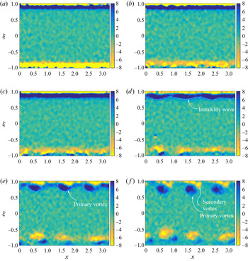
The growth of the disturbance can be observed from the vorticity contours obtained from the experimental data. During the after-deceleration phase of the flow, when the piston is already back to rest, perceptible instability waves start to appear. Thus, the after-deceleration flow field would be of interest and some of the vorticity contours from this duration are shown in figure 5. The figure shows a diametric plane of the whole pipe with the geometric dimensions scaled with the radius of the pipe, i.e.  $\xi = \pm 1$ refers to the top and bottom wall, respectively, and
 $x$ refers to the axial-flow direction. With the chosen coordinates of
 $(x, \xi )$, vorticity is positive in the
 $z$-direction, i.e.out of the plane of the image in the current context. Thus, the top (
 $+$ve
 $\xi$) and bottom (
 $-$ve
 $\xi$) planes have
 $z$-vorticity of oppositive signs (figure 6). Owing to problems such as particle coagulation, wall reflection, attenuation of the laser intensity and divergence of the laser sheet from top wall etc., the PIV results from the top wall region are much better than those obtained near the bottom wall, leading to differences in the bounds of vorticity distribution. However, the similarity can be observed in later phases of the flow when the instabilities develop into full grown vortices.
Vorticity contours (dimensional,  $s^{-1}$) obtained from the extracted velocity data are shown in (a–f) corresponding to six time instants starting from the piston stoppage time (
 $t_2$) with an interval of
 $\Delta t = 0.8\ \textrm {s}$, (a)
 $t_2$, (b)
 $t_2 + {\rm \Delta} t$, (c)
 $t_2 + 2\Delta t$, (d)
 $t_2 + 3\Delta t$, (e)
 $t_2 + 4\Delta t$ and (f)
 $t_2 + 5 \Delta t$.

Development of  $x$-averaged vorticity from the piston stoppage time (
 $t_2$) with an interval of
 $\Delta t = 0.8\ \textrm {s}$ (corresponding to (a–f) of figure 5).

As the piston deceleration time is short and the boundary layer is quite thin, no perceptible instability wave appears during the period. Thus, vorticity plots are shown starting from the instant that the piston stops, with a chosen time interval of  $\Delta t = 0.8\ \textrm {s}$. Observation of the vorticity field confirms the appearance of instability waves close to the pipe wall. These instability waves grow in strength and become more prominent by transforming into fully grown vortices. Gradually, the secondary vortices become visible and their interaction with the primary vortices leads to a breakdown of vortices. As the current study focuses on the linear stability aspect, an attempt is made to recognise the existence of instability waves and their growth.
4.1.1. Spatial DMD
During the comparison of the experimental velocity profiles with analytical solutions, it is observed that POD analysis may not be sufficient to isolate the base flow and disturbances when the instability waves gain comparable energy to that of base flow. The required analysis should rather use a mode decomposition which can rank the modes based on spatial evolution through wavenumber or wavelength. Here, spatial DMD is applied to the vorticity field at time instants where a perceptible instability wave has started appearing.
The dynamic spatial evolution of the system can be represented when each dataset holds the state information at individual spatial locations. Let, the velocity data at each axial location ( $x_i$) be represented by a vector
 $\boldsymbol{v}_{j}$. Then, if a linear operator
 $\boldsymbol {A}$ holds the dynamic information of the system, the system can be represented as
 \begin{equation} \boldsymbol{V}_2 = \boldsymbol{A} \boldsymbol{V}_1, \end{equation}
where  $\boldsymbol {V}_1 = [\boldsymbol {v}_1 \cdots \boldsymbol {v}_{n-1}]$ and
 $\boldsymbol {V}_2 = [\boldsymbol {v}_2 \cdots \boldsymbol {v}_n]$ (Duke, Soria & Honnery Reference Duke, Soria and Honnery2012). Each two subsequent datasets
 $\boldsymbol {v}_j$ and
 $\boldsymbol {v}_{j+1}$ are separated by the equal spatial interval
 $\Delta x$. The dynamical system can also be expressed using a companion matrix
 $\boldsymbol {S}$ and a residual vector
 $\boldsymbol {r}$ as (Schmid Reference Schmid2010)
 \begin{equation} \boldsymbol{AV}_1 = \boldsymbol{V}_2 = \boldsymbol{V}_1 \boldsymbol{S} + \boldsymbol{re}^{T}, \end{equation}
where  $\boldsymbol {e}$ is a unit vector. Again, as mentioned in Schmid (Reference Schmid2010), the eigenvalues of
 $\boldsymbol {S}$ approximate some of the eigenvalues of
 $\boldsymbol {A}$, i.e.
 $\boldsymbol {V}_2 \approx \boldsymbol {V}_1 \boldsymbol {S}$ can represent the system with associated residual error
 $\boldsymbol {r}$. Here, the spatial datasets
 $\boldsymbol {V}_1$ and
 $\boldsymbol {V}_2$ are available from experiment and can be used to extract the dynamic characteristics from the companion matrix
 $\boldsymbol {S}$.
Thus, with  $\boldsymbol {QR}$-decomposition of
 $\boldsymbol {V}_1$, i.e.
 $\boldsymbol {V}_1 = \boldsymbol {QR}$, the companion matrix
 $\boldsymbol {S}$ is defined as
 \begin{equation} \boldsymbol{S} = \boldsymbol{R}^{{-}1} \boldsymbol{Q}^{H} \boldsymbol{V}_2, \end{equation}
where  $\boldsymbol {Q}^{H}$ is the complex conjugate transpose of
 $\boldsymbol {Q}$. With singular value decomposition (SVD) of
 $\boldsymbol {R}$ as
 $\boldsymbol {R} = \boldsymbol {U} \varSigma \boldsymbol {W}^{H}$, the pseudo-inverse is calculated to be
 \begin{equation} \boldsymbol{R}^{{-}1} = \boldsymbol{W} \varSigma^{{-}1} \boldsymbol{U}^{H}. \end{equation}
Duke et al. (Reference Duke, Soria and Honnery2012) suggested the implementation a rank reduction by truncating the singular value matrix  $\varSigma$ based on the POD energy of the orthogonal modes of
 $\boldsymbol {V}_1$. This would cut off those modes having very low energy, generally associated with the noise, without affecting the leading eigenvalues of
 $\boldsymbol {S}$.
The complex eigenvalues of  $\boldsymbol {S}$ are solved (also known as the Ritz eigenvalues). These Ritz eigenvalues,
 $\{\phi _i\}$, provide the stability criteria determined by their relative distance from the unit circle and can be transformed to a complex stability plane through the logarithmic transformation,
 \begin{equation} \lambda_i = \log \phi_i / \Delta x. \end{equation}
The physical interpretation of the complex eigenvalue  $\lambda _i$ is that the real part,
 $\textrm {Re}(\lambda _i)=\sigma$, is the exponential growth or decay of the mode
 $i$ with the imaginary part,
 $\textrm {Im}(\lambda _i)=\alpha$, being the wavenumber. If temporal decomposition is required, the dataset is arranged by snapshots of equal time intervals, the imaginary part
 $\textrm {Im}(\lambda _i)$ would then provide the frequency of that particular mode
 $i$.
The results are shown in figure 7 using the vorticity fields as the snapshot data corresponding to the fourth and fifth sample data (d,e) of figure 5, and one in between the two. It shows the vorticity energy distribution with wavenumber,  $\alpha$, and the corresponding wave spectrum. The vorticity energy
 $E$ is defined as
 $E = \| \varOmega \|^{2}$, where
 $\varOmega$ is the azimuthal component of the vorticity and
 $\|\cdot \|$ represents the Euclidean norm. It is seen that only a few dominant modes are sufficient to define the wave structures present in the flow field. The plots are constructed from the 5–15 high energy modes, as part of the rank reduction suggested by Duke et al. (Reference Duke, Soria and Honnery2012). By decreasing the cut-off rank energy, the modes begin to group together, indicating convergence. Thus, it is observed that, even with the limited modes, the first few waveforms are recognised with confidence. The maximum amount of vorticity energy (in the current context, the energy of a vector field is represented by its Euclidean norm) is carried by a mode with zero wavenumber; suggesting that it corresponds to the mean-flow distribution. The second most energetic mode with a wavenumber of
 $\alpha \approx 200\ \textrm {m}^{-1}$ (i.e. wavelength of
 $\lambda \approx 0.03\ \textrm {m}$) represents the waveform visible in the vorticity plots. As instability waves become more prominent and visible in the vorticity plots, the spatial DMD analysis gives clear quantitative information regarding the waves that are present. To highlight this, the waveforms corresponding to the two most energetic DMD modes and their superimposition are shown in figure 8. These modes correspond to the time instant
 $t_2 + 4 \Delta t$ for which the vorticity plot is shown in (e) of figure 5. The first mode, which is the highest energy mode, represents the mean flow with
 $\alpha = 0$. The second mode is the most energetic perturbation mode (
 $\alpha \approx 200\ \textrm {m}^{-1}$). With superimposition of the two modes, a low-rank representation of the vorticity field is provided. Here, the DMD modes are suitably scaled to be in the range comparable to the experimental data. Thus, it is suggested that the primary instability wave can be identified and separated from the mean flow by use of spatial DMD analysis.
Vorticity energy and wave spectrum corresponding to each wave obtained from spatial DMD considering the most energetic modes. The three rows correspond to time instants  $t_2 + 3\Delta t$ (corresponding to fourth vorticity plot (
 $d$) of figure 5),
 $t_2 + 7/2\Delta t$ and
 $t_2 + 4\Delta t$ (corresponding to fifth vorticity plot (e) of figure 5) respectively. The number of modes considered are
 ${5, 7,\ldots, 15}$ represented by
 $\bullet$,
 $+$,
 $\times$,
 $\circ$,
 $\Box$ and
 $\diamond$, respectively.

Spatial DMD modes for vorticity field corresponding to time instant  $t_2 + 4 \Delta t$ (figure 5e): (a) first mode (
 $\alpha = 0$), (b) second mode (
 $\alpha \approx 200\ \textrm {m}^{-1}$) and (c) superimposition of first and second modes.

The energy growth or decay of each mode is observed in figure 9. As expected, with no further supply of energy, the flow field gradually loses its overall energy to viscous dissipation. This can be substantiated when the temporal DMD analysis is carried out in the next section. But, there is a slow growth to the instability waves, by drawing energy from the mean flow to maintain its existence and growth. The mean-flow distribution has been verified with first mode from POD analysis.
Vorticity energy development with time representing the growth of each spatial wave modes. The symbols  $\bullet$,
 $+$,
 $\times$,
 $\circ$ and
 $\Box$ correspond to time instants starting from
 $t_2 + 2\Delta t$ to
 $t_2 + 4 \Delta t$, corresponding to (c–e) of figure 5, with a time interval of
 $\Delta t / 2$, respectively.

The current analysis uses a spatial decomposition on the instantaneous snapshots of the velocity field, and thereby the vorticity distribution. The analysis allows us to recognise the mean-flow component and primary instability waveform, along with their associated energies, in the flow field. A visual observation of the mean-flow decay and the growth of a primary vortex is also made at a few time instants.
4.1.2. Temporal DMD
The temporal evolution of the flow field is also studied through a temporal DMD to gain further understanding. While spatial DMD was applied to a particular snapshot of the velocity field, temporal decomposition allows us to consider the velocity fields of the whole spatial domain as a single datum. The temporal sequence of the data fields, starting from a time instant after the piston stoppage to a time of interest, is used for analysing the dynamic evolution. Here, the time duration for which the analysis is carried out is from  $t_2 + 2\Delta t$ to
 $t_2 + 4\Delta t$, i.e. corresponding to (c–e) of figure 5. The instability waves seem to be fully grown in this phase of the flow and shedding of the vortices in the later phases may involve nonlinear phenomenon which is not in scope of the current analysis.
Energy and DMD spectra obtained from the temporal analysis are shown in figure 10. Spectra of the least-decaying modes are shown with associated energy, and the total number of modes used for analysis is increased to ensure consistency of the obtained result. The dynamic mode energy,  $E_k$, represents the kinetic energy of the mode and is defined, in a similar way as vorticity energy, with the Euclidean norm of velocity as
 $E_k = \|\boldsymbol {u}\|^{2}$, where
 $\boldsymbol {u} = [u\ v]^\textrm {T}$. Here,
 $u$ and
 $v$ represent axial and radial velocity, respectively. Figure 10 is also annotated with the two least-decaying DMD modes. Consistent values for the energy and growth rate of the DMD modes are obtained as the cut-off rank energy is reduced by including more orthogonal energy modes for analysis. This figure suggests that the mode marked as ‘1st mode’ carries the highest energy with the minimal decay. The other mode with a finite frequency marked as ‘2nd mode’ has a moderate energy, initially, but its decay rate seems to be an order higher than the first mode. The remaining high-frequency modes have comparatively low energy and very high decay rates. Hence, these low-energy modes can be associated with noises related to experiment and data acquisition.
Energy spectrum and DMD spectrum obtained from the temporal analysis considering the flow development between the time instants  $t_2+2\Delta t$ and
 $t_2 + 4\Delta t$, i.e. (c–e) of figure 5. Some of the least-decaying modes are shown in the plot while the number of energy modes used for analysis are
 ${5, 10,\ldots, 30}$ represented by
 $\bullet$,
 $+$,
 $\times$,
 $\circ$,
 $\Box$ and
 $\diamond$ respectively.

The focus is on the first two least-decaying modes, which are also high in energy (see figure 10). The highest-energy mode, shown in figure 11(a), is obtained using a total of 25 modes. This mode is found to be associated with approximately zero frequency and the corresponding decay rate of this mode is less than  $0.1\ \textrm {s}^{-1}$. As the duration of the temporal analysis is
 $2 \Delta t = 1.6\ \textrm {s}$, the mode does not lose more than 20 % of its energy during this period. By comparison with the above, the second mode carries a frequency of approximately 4 Hz and its decay rate is approximately
 $1.2\ \textrm {s}^{-1}$. Thus, within an order of magnitude, it can be stated that when the perceptible instability wave appears at
 $t_2 + 4\Delta t$ ((e) of figure 5), this mode has approximately only 15 % remaining of its initial energy (which subsequently vanishes rapidly). Thus, temporal DMD analysis can be used to locate the mode that would decay the least compared with any other mode in the interval of analysis. This mode may be a superposition of the base flow and perturbations, and is the most sustained structure of this transient flow.
DMD modes obtained from the analysis considering the flow development between the time instants  $t_2+2\Delta t$ and
 $t_2 + 4\Delta t$, i.e. (c–e) of figure 5. The DMD modes are obtained with 25 high-energy modes being used for analysis. (a) First mode, (b) second mode.

After rejecting any significance of the second least-decaying mode in the context of the current study, focus can be shifted to the first mode shown in figure 11(a). This mode carries the maximum energy, decays in the slowest manner over the analysis period and, thus, becomes a sustained structure as the other modes vanish quickly. Because temporal mode decomposition is based on frequency, and the flow dynamics of the discussed phenomena lack periodicity, the current analysis does not allow us to separate out evolution of mean flow and perturbation quantities. The overall combined energy of mean flow and the perturbation decays quite slowly, suggesting that the loss of the mean-flow energy is compensated for by the growth of the perturbation. In other words, it can be stated that the instability wave is drawing most of its energy from the mean flow.
4.2. Quasi-steady stability results
It is seen during the velocity profile comparison in the previous section that deceleration in piston motion introduces a reverse-flow region with inflectional velocity profile. The flow development after piston stoppage is transient in nature and has similarity to the suddenly blocked flow in a duct (Nayak & Das Reference Nayak and Das2017). A quasi-steady approach, based on modal analysis, has been a classical tool for the study of instability in such flows (Das & Arakeri Reference Das and Arakeri1998; Ghidaoui & Kolyshkin Reference Ghidaoui and Kolyshkin2002). Thus, following the idea, the base flow is considered to be frozen at each time instant and linear stability analysis is attempted on corresponding velocity profiles. The results show that the profiles are self-similar and that the stability characteristics are mainly controlled by the velocity difference,  $\Delta u = u_{max}-u_{min}$ and boundary-layer thickness,
 $\delta$, similar to inviscid instability in parallel shear flows. This is reflected in figure 12, where the instantaneous growth rates (
 $c_i$) of the most unstable mode, normalised by
 $\Delta u$, are plotted with scaled wavenumber (
 $\alpha _\delta = \alpha \delta$) for different time instants after the piston stoppage.
Variation of normalised instantaneous growth rates ( $c_{i, \Delta u} = c_i/\Delta u$) of the most unstable mode with wavenumber (
 $\alpha _\delta = \alpha \delta$) for velocity profiles corresponding to time instants after the piston has stopped. Time instants are considered starting from the piston stoppage time (
 $t_2$) with an interval (
 $\Delta t = 0.8\ \textrm {s}$) represented by
 $\bullet$,
 $+$,
 $\times$,
 $\circ$ and
 $\Box$ respectively. (a) Plot of
 $c_{i,\Delta u}$ versus
 $\alpha _\delta$: instantaneous results using analytical velocity profiles. (b) Plot of
 $\alpha _\delta c_{i,\Delta u}$ versus
 $\alpha _\delta$: corresponding to (a). (c) Plot of
 $c_{i,\Delta u}$ versus
 $\alpha _\delta$: instantaneous results using experimental velocity. (d) Plot of
 $\alpha _\delta c_{i,\Delta u}$ versus
 $\alpha _\delta$: corresponding to (c). (e) Scatter plot of the maximum instantaneous growth rate and corresponding wavenumber for both analytical (
 ${\bigtriangleup}$) and experimental (
 ${\bigtriangledown}$) velocity profiles.

The behaviour of the instantaneous growth-rate curves, obtained from the experimental velocity profiles, seems to be different from that obtained from the analysis of analytical profiles. However, closer inspection of figure 12 reveals that, except the first two velocity profiles, all other profiles show similar stability characteristics as seen in the analytical results. The growth-rate patterns show similarity when scaled with the instantaneous velocity difference and boundary-layer thickness. This is a characteristic observed in inflectional velocity profiles with reverse flow (Das & Arakeri Reference Das and Arakeri1998). It suggests that the flow development during this period is a result of viscous diffusion only and the nature of involved flow instability is inflectional in nature. The appropriate characteristic velocity and length scales are the velocity difference and the boundary-layer thickness, respectively.
4.3. Optimal energy growth
In the previous section, it is seen that the flow under consideration exhibits the potential for perturbation growth. This can be observed from the instantaneous growth-rate curves, shown in figure 12, obtained through quasi-steady analysis. These growth-rate curves show a similar nature when the growth rates are normalised (Das & Arakeri Reference Das and Arakeri1998; Ghidaoui & Kolyshkin Reference Ghidaoui and Kolyshkin2002). However, with decaying flow, the velocity scale  $\Delta u$, i.e.instantaneous velocity difference, and, in turn, growth-rate decrease over time. Again, the most sensitive wavenumber,
 $\alpha$, with maximum potential for instability also changes over the duration with the growth of boundary layer
 $\delta$, which is used to scale wavenumber to
 $\alpha _\delta$. Thus, the prediction to identify the instability wave that would appear as the consequence of instability in this decaying flow would require a different approach. One such approach is to use non-modal stability analysis to obtain the optimal perturbation and corresponding optimal growth over an analysis period.
Non-modal stability analysis deviates from the typical normal mode approaches, which provide asymptotic long-term stability characteristics of the flow, by considering the transient growth of a perturbation over a finite time interval. In the case of steady flow, it can provide the algebraic growth of perturbation which can be substantial even when there is no unstable mode present in normal mode analysis (Farrell Reference Farrell1988; Butler & Farrell Reference Butler and Farrell1992; Bergström Reference Bergström1993; Schmid & Henningson Reference Schmid and Henningson1994). In the case of time-dependent base flow, such as the decaying flow under discussion, where the asymptotic long-term behaviour does not make physical sense, non-modal stability analysis can be used to analyse the changing base flow (Nayak & Das Reference Nayak and Das2017).
This concept and its implementation are borrowed from Schmid (Reference Schmid2007) and is applied to the current problem. Similar implementation of optimal energy growth with an explicit transient technique is available in Jewell & Denier (Reference Jewell and Denier2006). The receptivity study pertaining to external forcing, such as noise, is not considered in this study. Rather, the focus is on determination of the optimal initial perturbation that provides the maximum perturbation energy growth over the analysis domain. Thus, the formulation seems to be an optimisation problem with the perturbation state vector  $\boldsymbol {q}$ over the initial perturbation
 $\boldsymbol {q}(0)$ such that the energy growth,
 $G(T)$, over the analysis interval
 $[T_0=t_2, T=t_2+4\Delta t]$ is maximised. Thus, the functional
 $G(T)$ defined over the space of state vector
 $\boldsymbol {q}$ as
 \begin{equation} G(T) = \frac{E(T)}{E(0)} = \frac{\| \boldsymbol{q}(T) \|_E^{2}}{\| \boldsymbol{q}(0) \|_E^{2}} \end{equation}
needs to be maximised against the spatial distribution of the initial perturbation  $\boldsymbol {q}(0)$, where
 $\|. \|_E$ represents the energy norm.
In the current context, the state vector is the perturbation quantity represented by  $\boldsymbol {q} = [\varPhi \ \varPsi ]^\textrm {T}$, where
 $\varPhi$ and
 $\varPsi$ are the transformed radial velocity and radial vorticity, respectively, as (Burridge & Drazin Reference Burridge and Drazin1969; Nayak & Das Reference Nayak and Das2019)
 \begin{equation} \varPhi ={-}\textrm{i} r v \quad \mbox{and} \quad \varPsi = (\alpha rw -nu)k^{2}r^{2}, \end{equation}
where  $u$,
 $v$ and
 $w$ are the perturbation velocities and
 $r$ represents the radial coordinate. Here,
 $\alpha$ and
 $n$ represent the streamwise wavenumber and discrete azimuthal wavenumber, respectively, with
 $k^{2} = \alpha ^{2} + n^{2}/r^{2}$. The energy norm
 $\| q \|_E$ is defined with the kinetic energy density as
 \begin{equation} \|\boldsymbol{q}\|_E^{2} = \int_{0}^{1}\left[|u|^{2} + |v|^{2} + |w|^{2} \right] 2{\rm \pi} r \,\textrm{d}r. \end{equation}
Details about the form of perturbation state vector  $\boldsymbol {q}$, the governing perturbation equations and the solution technique are presented in Nayak & Das (Reference Nayak and Das2019).
The time interval chosen for analysis starts from the piston stoppage time to a time instant of interest, where the instability waves are evident. From the vorticity contours obtained from the experimental data and shown in figure 5, the suitable interval is set to be  $[t_2, t_2+4\Delta t]$, i.e. (a–e) of figure 5.
The implemented numerical scheme is capable of handling both axisymmetric and non-axisymmetric perturbations. But, it is observed that the axisymmetric mode ( $n=0$) is dominant as the boundary layer is small for the given problem (Ghidaoui & Kolyshkin Reference Ghidaoui and Kolyshkin2002). Thus, the optimal perturbations corresponding to various wavenumbers,
 $\alpha _R = \alpha R$, and
 $n=0$ are obtained and their energy growth over the analysis domain is shown in figure 13. The analysis is carried out considering both the analytically and experimentally obtained velocity profiles. The theoretical velocity profiles have large reverse-flow magnitude and similar boundary layers compared with those obtained experimentally. The optimal growths obtained for the theoretical profiles are comparatively higher. This inference is consistent with the observation made in Das & Arakeri (Reference Das and Arakeri1998) where the local Reynolds number, based on velocity difference and boundary-layer thickness, is a critical parameter for instability of an inflectional velocity profile. In their study, growth rates scale with velocity difference
 $\Delta u$. Comparison between them is shown in figure 14(a) for a chosen value of
 $\alpha _R=8$ taken from the observation of figure 13. The most unstable mode, obtained from the quasi-steady analysis, is also time integrated over the decay of the base flow; its energy growth is plotted (represented by the dashed lines) in the same figure. The overall growth achieved by the optimal mode is some order higher than that which can be achieved by the most unstable normal mode. Thus, the maximum growth that is achieved over the analysis duration is presented in figure 14(b). The wavenumber is normalised with the boundary-layer thickness,
 $\delta _2$, at the piston stoppage time. It provides an estimate of the range of sensitive wavenumbers which are approximately the same for both analyses. Hence, the analysis suggests that there is an intermediate wavenumber which is capable of providing the maximum perturbation energy growth.
Energy growth  $G(t)$ of the optimal perturbations obtained for
 $n=0$ and various wavenumbers
 $\alpha _R = 5,6, \ldots, 10$ represented by
 $\bullet$,
 $+$,
 $\times$,
 $\circ$,
 $\Box$ and
 $\diamond$, respectively. Optimal perturbation is determined by maximisation of energy
 $E(T)/E(T_0)$ in an interval
 $[T_0=t_2, \ T=t_2+4\Delta t]$, i.e. (a–e) of figure 5. (a) Results with analytical velocity profiles and (b) results with experimental velocity profiles

Comparison of energy growths of the optimal perturbations obtained considering the analytical and experimental velocity profiles denoted by  $\circ$ and
 $+$, respectively. Optimal perturbation is determined by maximisation of energy
 $E(T)/E(T_0)$ in an interval
 $[T_0=t_2, T=t_2+4\Delta t]$, i.e. (a–e) of figure 5. (a) Results of the optimal mode (solid line) compared with that of the most unstable mode (dashed line) obtained from quasi-steady normal-mode analysis for
 $\alpha _R=8$. (b) Variation of total energy growth
 $G(T)$ over the analysis interval with normalised wavenumber using boundary-layer thickness,
 $\delta _2$.

From the previous analysis, the order of maximum perturbation energy growth obtained is approximately  $10^{4}$. Perturbation growth, by itself, is not useful and there is a need to compare it with the development/decay of the mean flow. Figure 15 shows the perturbation energy growth (
 $G(t$)) and the mean-flow kinetic-energy decay (
 $\|U(t)\|^{2}/\|U(0)\|^{2}$, where
 $\|U\|^{2} = \int _{0}^{1} |U|^{2} \ 2{\rm \pi} r \,\textrm {d}r$), plotted for two chosen wavenumbers
 $\alpha _R=8$ and
 $10$. The results suggest that the perturbation energy can be comparable to, or more than, the mean-flow energy within a short interval and becomes manyfold within the analysis period. Thus, considering all the previously discussed analyses, it can be established that it is the transient growth of the optimal perturbation which is responsible for the observed instability wave. Optimal mode is formed with the superposition of a finite number of least-stable eigenmodes. Though the radial distribution of the most-stable eigenmode and the optimal modes are different, the maximum energy concentration in both the cases occurs at a similar location (as shown in figure 16). Thus, it is postulated that the most unstable mode is one of the major contributors to the optimal mode. This has also been observed for the impulsively blocked channel flows in Nayak & Das (Reference Nayak and Das2017).
Growth of perturbation energy (shown with symbols  $+$ and
 $\times$) compared with mean-flow energy decay (shown with symbol
 $\circ$) over the same analysis interval
 $[t_2, t_2+4\Delta t]$ for
 $\alpha _R=8$ and
 $10$ considering (a) analytical and (b) experimental velocity profiles.

Radial distribution of transformed variable representing radial velocity,  $\varPhi (r)$ (
 ${=}-\textrm {i} r v$, where
 $v$ is the radial component of perturbation velocity), of the optimal mode (solid line) of non-modal analysis and the most unstable mode at piston stoppage time (dashed line) obtained from the quasi-steady modal analysis. Results are plotted for a chosen value of
 $\alpha _R = 8$. The line joining the triangular-shaped markers show the change in inflection-point locations.

5. Conclusions
Flow instability in a transient pipe flow is studied with both experimental and numerical approaches. Experimentation is carried out with an unsteady pipe flow devised to emulate the suddenly blocked pipe flow. PIV measurement provides the velocity-field data which are analysed to obtain the coherent wave structures and their associated energies. Both experimental and approximated analytical velocity profiles are used for the theoretical study of the flow mechanism through linear stability. POD analysis ranks the modes based on energy, whereas spatial DMD demarcates the modes based on wavenumber. The nonlinear interaction of primary and secondary vortices will be studied in detail separately, and is kept for future work.
Application of modal decomposition to experimental data justifies the view that only a few number of modes are involved in the development of the flow field. One of the modes being the mean flow with the highest energy, losing its energy both in viscous dissipation and supplying energy to sustain the growth of the instability. The analysis enables us to isolate the mean flow and primary instability modes from other modes originating from the noise and oscillations.
Linear stability analysis on this decaying flow is carried out to establish the mechanisms involved in the flow development. Quasi-steady analysis establishes the fact that the flow development after the piston stoppage is driven mostly by viscous diffusion. The efficacy of non-modal analysis for this case is apparent owing to the decaying nature of the base flow. Thus, the optimal perturbation responsible for maximum energy growth and the range of sensitive wavenumbers are obtained in the process. The comparative study of both optimal and most unstable modes suggests that the transient energy growth of the optimal mode is mainly responsible for the observed instability.
Declaration of interests
The authors report no conflict of interest.