1 Introduction
Canopies are essentially porous obstructions consisting of distributed drag elements that cause a partial blockage against the incoming flow. Depending on the vertical dimensions of canopy patches,
 $h$
, relative to the total flow depth,
 $H$
, they can be classified into emergent canopies occupying the whole flow depth (
 $h\geqslant H$
), submerged canopies (
 $h<H$
, bottom-mounted) and suspended canopies (
 $h<H$
, surface-floating). Compared to the first two types, suspended canopies have received less attention. Common examples include floating vegetation in river flows and kelp forests in the coastal ocean, which are usually found to be in the form of localized groups.
Suspended vegetation patches are ecologically and structurally important. They may lead to adverse effects, such as destabilizing dissolved oxygen, shading out crucial shallow-water fish habitat, obstructing waterways and navigational channels, and blocking agricultural and municipal water intakes. However, suspended vegetation also has positive aspects. For example, Eichhornia crassipes is a rich source of biogas due to its abundant nitrogen and fast rate of development (Wolverton & McDonald Reference Wolverton and McDonald1981). In addition, such vegetation can be used in wastewater treatment systems by absorbing organic materials and heavy metals (Xavier, Janzen & Nepf Reference Xavier, Janzen and Nepf2018). Proper design of these aquacultural and water-quality controlling systems requires a comprehensive understanding of the complex interplay between flow forcing and canopy architecture as well as the hydrodynamically mediated biological processes. Applications include the modification of nutrient uptake due to changing in-canopy currents, and patch-to-patch interactions depending on the canopy-induced adjustment of flow pathways.
Circular cylinders with their axes parallel to the vertical direction are often used to model the constituent vegetation stems due to the shape similarity and well-known flow responses (Zdravkovich Reference Zdravkovich1997). The current literature pertaining to canopy patches mainly focuses on the emergent case (Nicolle & Eames Reference Nicolle and Eames2011; Chen et al.
Reference Chen, Ortiz, Zong and Nepf2012; Zong & Nepf Reference Zong and Nepf2012; Chang & Constantinescu Reference Chang and Constantinescu2015). For this case, the flow can be considered to be predominantly two-dimensional, with minor variation of the mean flow along the vertical direction. For such a case, the planar cylinder configuration uniquely dictates the flow structure. For a fixed ratio between diameters of the patch (
 $D$
) and its constituent cylinders (
 $d$
), a common indicator of canopy density is the solid volume fraction
 $\unicode[STIX]{x1D719}$
, which is defined as the ratio of the plane area occupied by all the individual cylinders within the patch to the base area of the patch. The two-dimensional direct numerical simulation (DNS) study by Nicolle & Eames (Reference Nicolle and Eames2011) has shown that, depending on the canopy density, three regimes can be identified: (i) For small
 $\unicode[STIX]{x1D719}$
, each cylinder behaves as an isolated body and the wake of the group is composed of well-identifiable individual wakes. (ii) For moderate
 $\unicode[STIX]{x1D719}$
, there is a longitudinally uniform steady wake region sandwiched by lateral separated shear layers. The steady wake is stabilized by the streamwise bleeding flow through the patch interior, whose strength diminishes with increasing patch density. (iii) At large
 $\unicode[STIX]{x1D719}$
, the patch mimics the behaviour of a solid body in terms of both drag and wake characteristics.
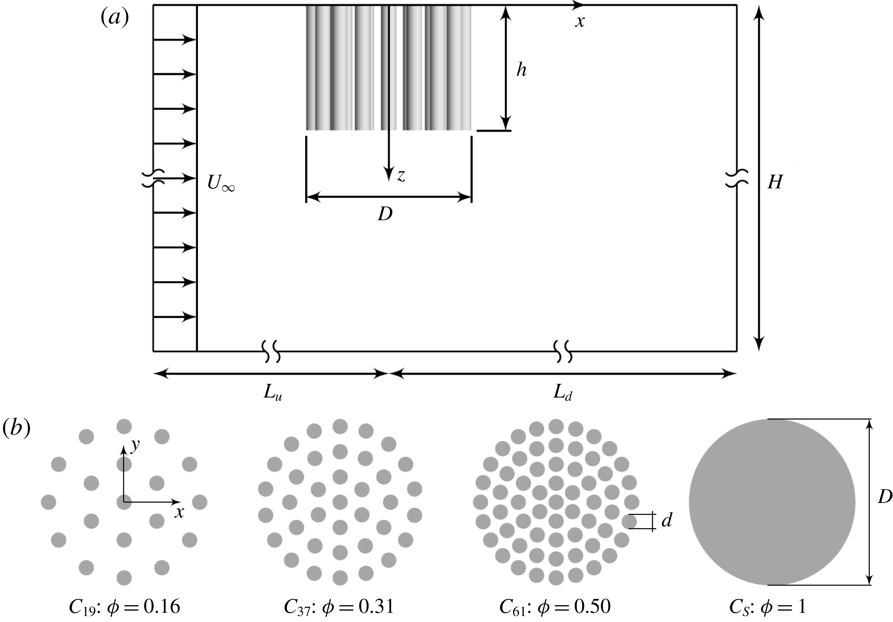
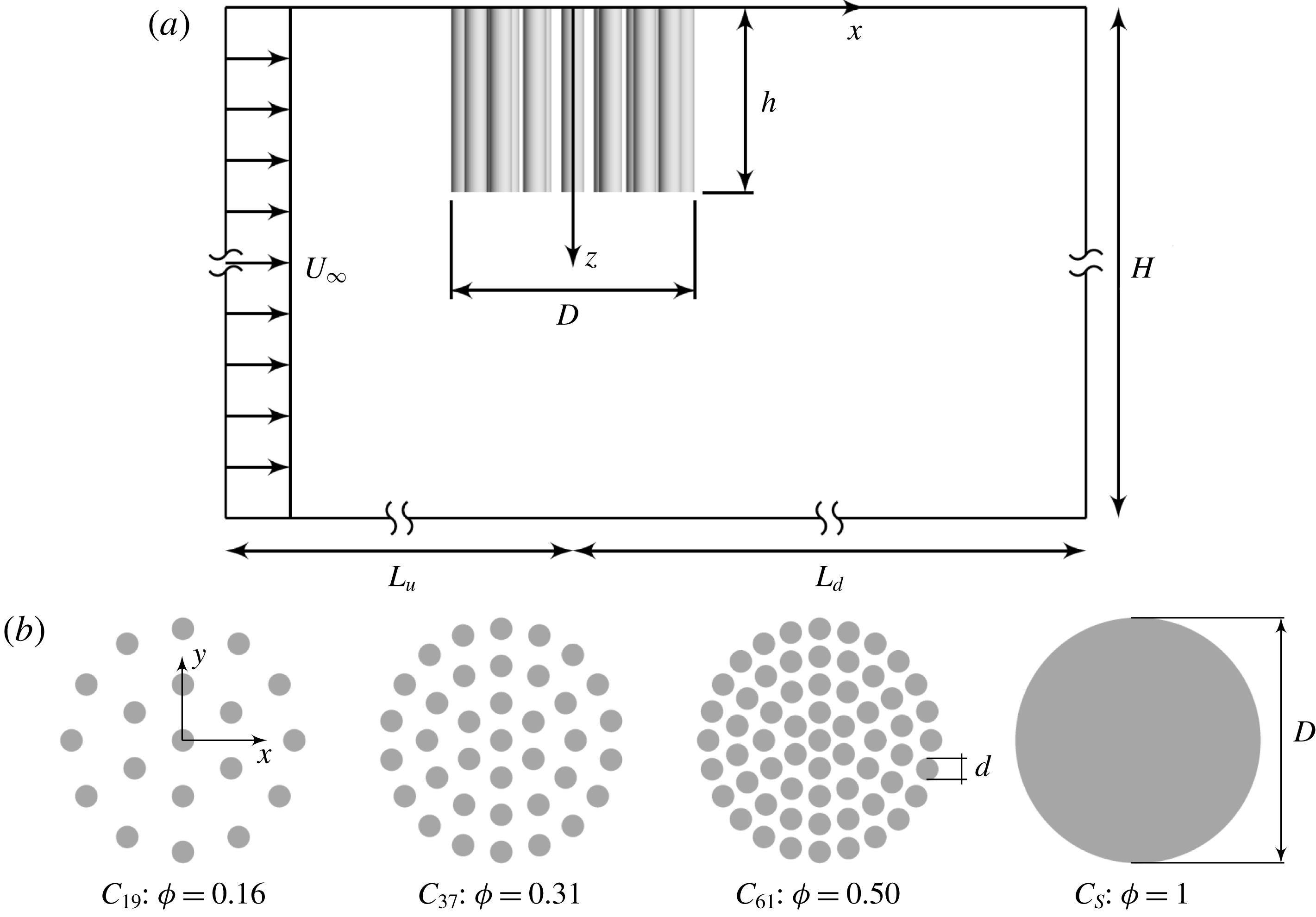
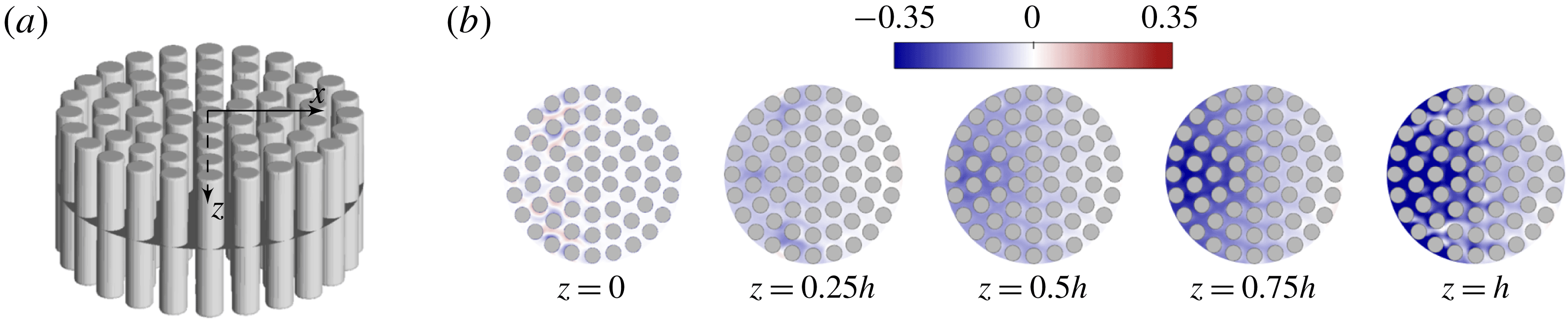
(a) Sketch of the computational domain (side view, not to scale). The suspended patch (diameter,
 $D$
, and height,
 $h$
) extends downwards from the domain top boundary in deep water with a total depth of
 $H=36h$
which varies between cases (to maintain a constant
 $H/h=36$
). The origin of the coordinate system is located at the centre of the patch top surface, and
 $z$
is pointing downwards. The domain width (out of plane) is
 $B=11D$
. The distances from the patch centre to the upstream and downstream domain extremities are
 $L_{u}=9D$
and
 $L_{d}=45D$
, respectively. (b) Plan view of cylinder configurations.
For partial-depth canopy patches (
 $h<H$
, either bottom-mounted or surface-suspended), however, it is conceivable that the vertical dimension of the patch is no longer irrelevant due to its capacity in modifying the three-dimensional features initiated near the patch free end and the resulting wake structure (Chen, Jiang & Nepf Reference Chen, Jiang and Nepf2013). For canopies spanning the whole channel width, the effect of submergence ratio,
 $h/H$
, has been investigated in a few studies by varying the total flow depth with a fixed canopy height
 $h$
(Nepf & Vivoni Reference Nepf and Vivoni2000; Hamed et al.
Reference Hamed, Sadowski, Nepf and Chamorro2017). Essentially, the ratio
 $h/H$
reflects the relative importance of driving forces: the longitudinal pressure gradients and the turbulent stress at the canopy free end (Nepf Reference Nepf2012). However, for finite patches with limited length and width,
 $h/H$
provides incomplete information about the local topographic feature of the obstruction due to the possible flow pathway horizontally around the patch in addition to the overflow. In this case, although varying either the patch height or the flow depth may result in similar variations of the submergence ratio
 $h/H$
, they have dynamically different effects on the flow.
In this paper, we present results from large-eddy simulations (LES) of a uniform incident flow impinging on a cylindrical canopy patch suspended in deep water. Figure 1 shows the main geometric and flow parameters of the problem configurations investigated in this study. The unconfined condition (
 $h/H\ll 1$
) is assumed to exclude the effects of submergence ratio and bottom friction. The key research question we aim to answer is the effect of the geometrical characteristics of a canopy patch on the mean flow dynamics. For the suspended cylindrical patch shown in figure 1, apart from the canopy density
 $\unicode[STIX]{x1D719}$
, we include an additional geometric parameter, the patch aspect ratio
 $AR=h/D$
, in order to characterize the relative patch dimensions between the vertical and horizontal directions. Despite the apparent importance of
 $AR$
, very limited existing studies can be found in the literature. Therefore, a systematic investigation of the near-wake structure in the
 $\unicode[STIX]{x1D719}$
–
 $AR$
parameter space is lacking. Such an investigation has broader practical relevance. For instance, the modelling of canopy patches with different
 $\unicode[STIX]{x1D719}$
–
 $AR$
combinations can mimic different stages of the root system of floating vegetation in order to assist in predicting local flow conditions and thus level of nutrient uptake.
Particular attention will be paid to answer the following overarching question: How does the incoming flow adjust its local and global pathway upon interaction with a canopy patch whose geometry varies in the
 $\unicode[STIX]{x1D719}$
–
 $AR$
parameter space? Specifically, how is the upstream undisturbed flow redistributed into penetrating through, horizontally around and vertically beneath the patch (i.e. global flow diversion), and how is the flow entering the patch redistributed towards the streamwise, lateral and vertical directions as bleeding flows (i.e. local flow bleeding)? Previous studies have shown that suspended canopies cause flow disturbances, such as reduced velocities within the canopy (Plew Reference Plew2011). The effect of patch density
 $\unicode[STIX]{x1D719}$
on the bleeding flow has been investigated by Taddei, Manes & Ganapathisubramani (Reference Taddei, Manes and Ganapathisubramani2016) and Tseung, Kikkert & Plew (Reference Tseung, Kikkert and Plew2016), but with a constant
 $AR$
. The present study aims to shed some light on this three-dimensional flow adjustment, which is expected to have important implications for the design of multi-patch systems (e.g. single-patch geometry and patch-to-patch arrangement) for applications such as the optimization of biomass productivity or the efficiency of floating wastewater treatment systems.
The layout of this paper is as follows. Section 2 describes the numerical methodology, validation of the LES code, and the simulation set-ups of the parametric study. Section 3 provides an overview of the flow features as a function of the patch density and aspect ratio. Section 4 presents the detailed vertical motions inside the patch to explain the observed flow structure in § 3. Section 5 is devoted to the three-dimensional flow bleeding dynamics (i.e. the local flow bleeding) within the
 $\unicode[STIX]{x1D719}$
–
 $AR$
parameter space. Section 6 is dedicated to the global flow diversion through, around and beneath the canopy patch, and relates it to § 5. Section 7 discusses the bulk drag coefficients of the canopy patches. Finally, conclusions are drawn in § 8.
2 Numerical methodology, validation and simulation set-up
2.1 Numerical methodology
Large-eddy simulation is employed in this study, where the larger three-dimensional unsteady turbulent motions are directly represented, while the effects of the smaller-scale motions are modelled. Spatial filtering operation is applied to the governing equations, splitting the velocity
 $\boldsymbol{U}$
into a filtered field,
 $\overline{\boldsymbol{U}}$
, and a subgrid-scale (SGS) field,
 $\boldsymbol{u}^{\prime }$
. The LES-filtered momentum equation is given in tensor notation by
 $$\begin{eqnarray}\displaystyle \frac{\unicode[STIX]{x2202}\overline{U}_{i}}{\unicode[STIX]{x2202}t}+\frac{\unicode[STIX]{x2202}\overline{U}_{i}\overline{U}_{j}}{\unicode[STIX]{x2202}x_{j}}=-\frac{1}{\unicode[STIX]{x1D70C}}\frac{\unicode[STIX]{x2202}\overline{p}}{\unicode[STIX]{x2202}x_{i}}+\unicode[STIX]{x1D708}\frac{\unicode[STIX]{x2202}^{2}\overline{U}_{j}}{\unicode[STIX]{x2202}x_{j}\unicode[STIX]{x2202}x_{j}}-\frac{\unicode[STIX]{x2202}\unicode[STIX]{x1D70F}_{ij}^{SGS}}{\unicode[STIX]{x2202}x_{j}}, & & \displaystyle\end{eqnarray}$$
subject to the filtered continuity equation
 $$\begin{eqnarray}\displaystyle \frac{\unicode[STIX]{x2202}\overline{U}_{i}}{\unicode[STIX]{x2202}x_{i}}=0, & & \displaystyle\end{eqnarray}$$
where
 $\overline{U}_{i}$
are the Cartesian components of the filtered velocity field,
 $\overline{p}$
is the filtered pressure,
 $\unicode[STIX]{x1D70C}$
is the fluid density,
 $\unicode[STIX]{x1D708}$
is the kinematic viscosity, and
 $\unicode[STIX]{x1D70F}_{ij}^{SGS}=\overline{U_{i}U_{j}}-\overline{U}_{i}\overline{U}_{j}$
is the subgrid-scale stress tensor. Time is represented by
 $t$
and the index
 $i=1,2,3$
indicates the
 $x$
(streamwise),
 $y$
(lateral) and
 $z$
(vertical) directions, respectively.
The governing equations are solved using the finite-volume computational fluid dynamics (CFD) software, FLOW-3D, developed by Flow Science, Inc., Santa Fe, New Mexico. The closure of the SGS stress tensor
 $\unicode[STIX]{x1D70F}_{ij}^{SGS}$
in (2.1) is solved using the standard Smagorinsky model (Smagorinsky Reference Smagorinsky1963). The unique volume-of-fluid (VOF) method (Hirt & Nichols Reference Hirt and Nichols1981) of FLOW-3D provides an accurate way to track and locate the free surface or fluid–fluid interface using structured meshes, which consists of three ingredients: a scheme to locate the surface; an algorithm to track the surface as a sharp interface moving through a computational grid; and a means of applying boundary conditions at the surface. Besides this, the Fractional Area–Volume Obstacle Representation (FAVOR™) technique (Hirt Reference Hirt1993) used exclusively in FLOW-3D enables the model to change the embedded geometry realistically without changing the mesh, which is considered superior for the present study, where a parametric study of geometric variation is undertaken. The second-order, monotonicity-preserving upwind-differencing method (van Leer Reference van Leer1977) is applied to approximate the momentum advection. The pressure is solved implicitly using the generalized minimum residual algorithm (GMRES) due to its high accuracy, rapid convergence and parallel efficiency (Yao Reference Yao2004).
2.2 Model validation
FLOW-3D has been extensively validated for various flow–obstacle interaction problems. Zhou & Venayagamoorthy (Reference Zhou and Venayagamoorthy2017) validated the propagation dynamics of intrusive gravity currents predicted by FLOW-3D against experimental data and investigated their interaction with a bottom-mounted obstacle. Zhou et al. (Reference Zhou, Cenedese, Williams, Ball, Venayagamoorthy and Nokes2017) studied the propagation of gravity currents over a submerged canopy composed of circular cylinders. LES using the same code successfully reproduced the experimentally measured front speed and mixing pattern of the gravity current as it interacts with the canopy.
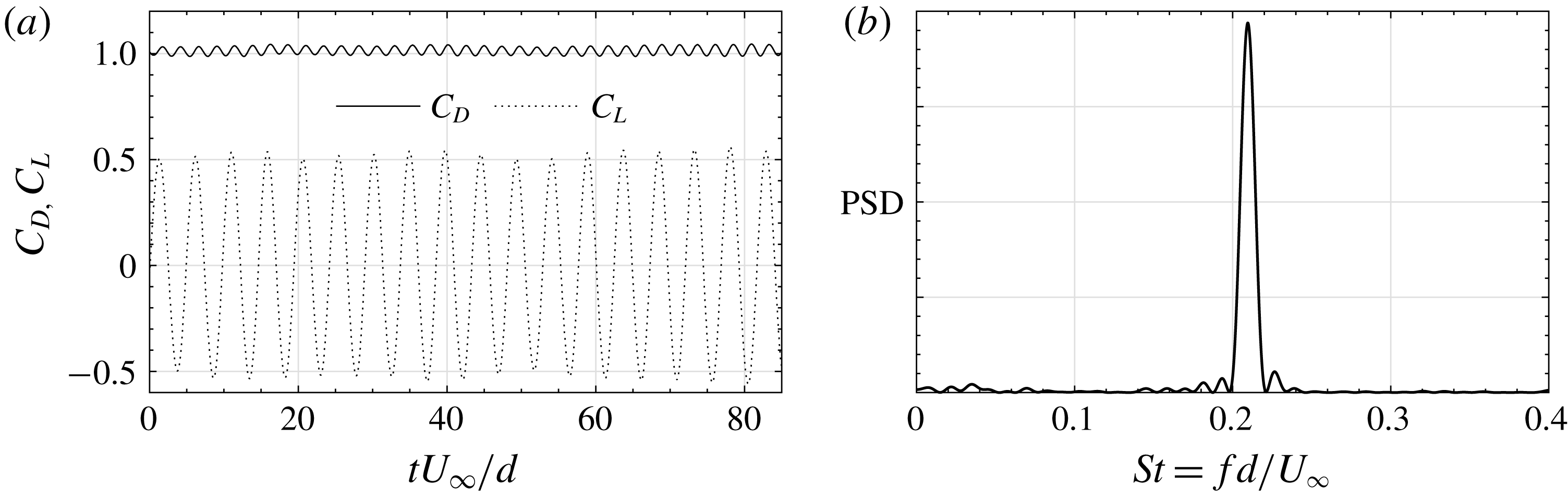
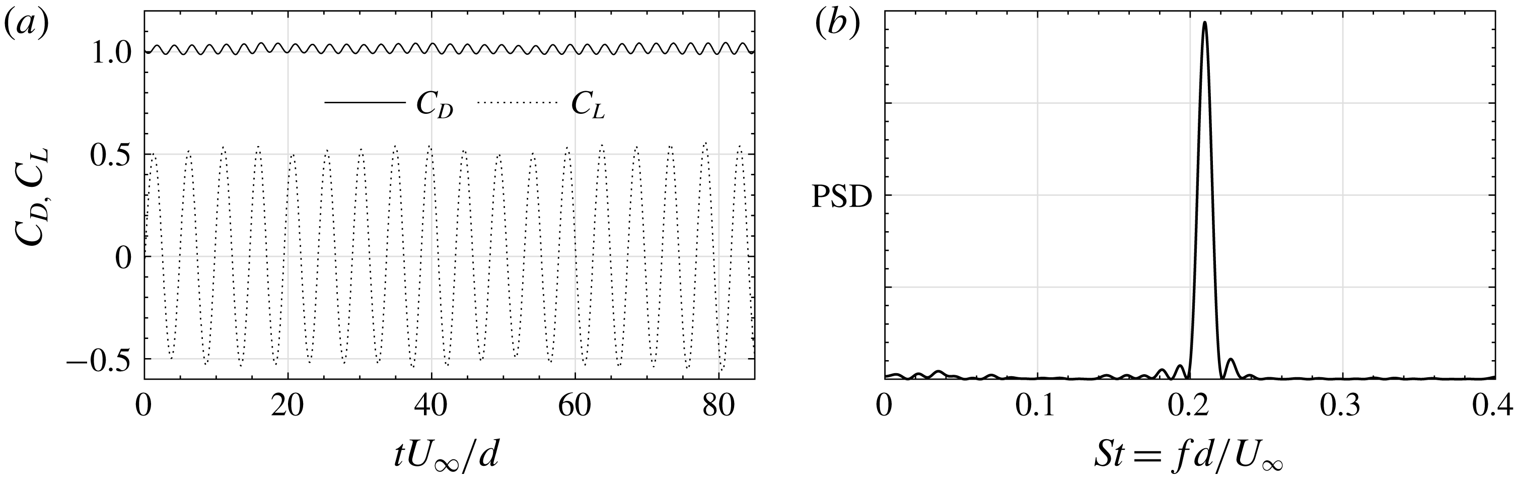
In this paper, a set of additional simulations were conducted to validate the numerical model. Firstly, the canonical case of flow past an infinitely long solid circular cylinder with
 $Re_{d}=U_{\infty }d/\unicode[STIX]{x1D708}=1000$
was simulated, where
 $U_{\infty }$
is the free-stream streamwise velocity and
 $d$
is the cylinder diameter. A Cartesian mesh with a resolution of
 $0.125d$
was used throughout the near-wake region. The time-averaged drag coefficient predicted by the present LES (
 $C_{D}=1.01$
, figure 2
a) agrees well with the value of 1 reported in experiments (Zdravkovich Reference Zdravkovich1997). The Strouhal number was observed to be
 $St=0.209$
(figure 2
b), which is also very close to the experimental measurements of 0.21 (Zdravkovich Reference Zdravkovich1997).
Model validation: flow past an infinitely long solid circular cylinder at
 $Re_{d}=U_{\infty }d/\unicode[STIX]{x1D708}=1000$
. (a) Time history of the drag and lift coefficients. (b) Power density spectrum (PSD) of the lift coefficient, where
 $f$
is the vortex shedding frequency.
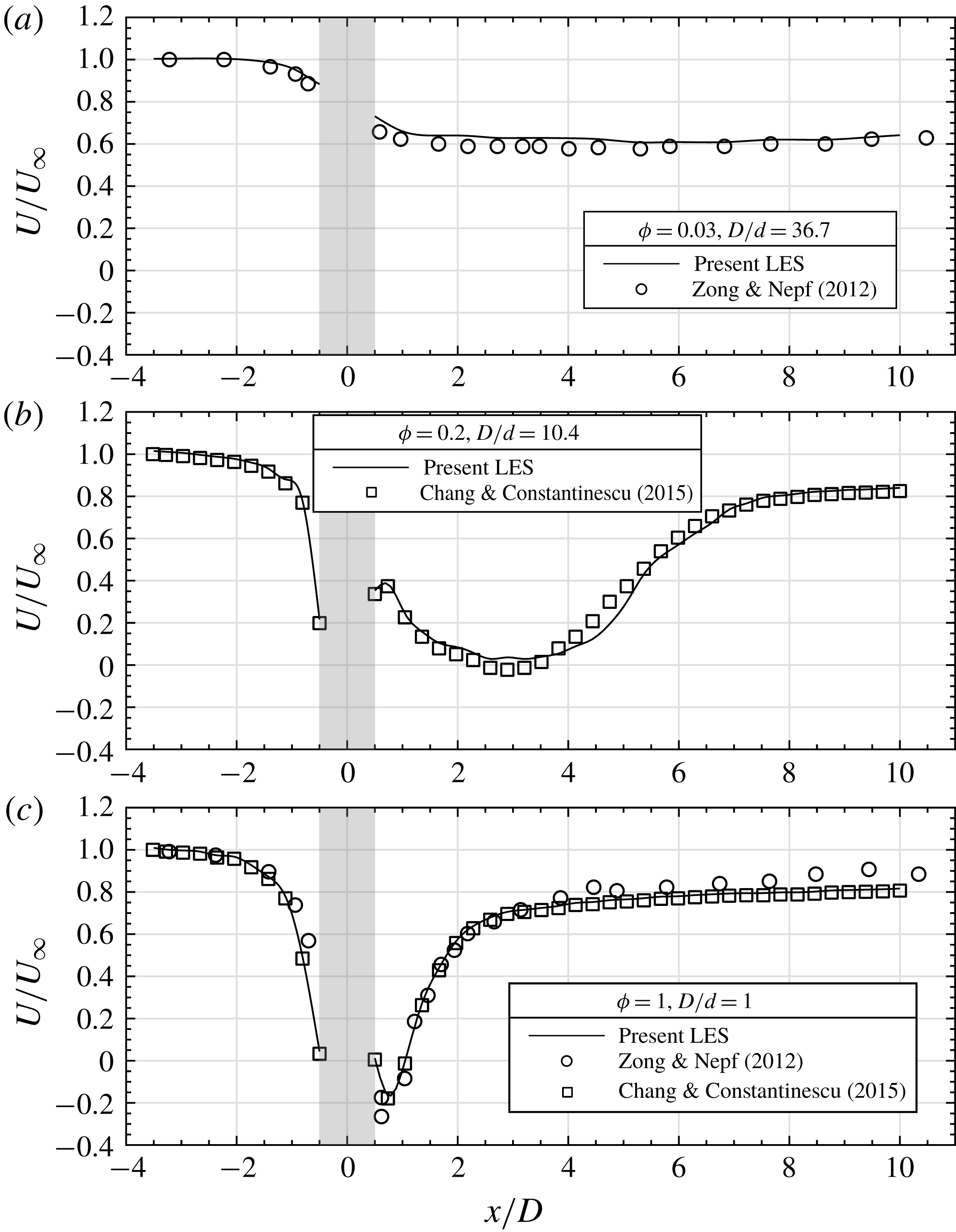
Model validation: flow past an emergent cylindrical canopy patch: (a)
 $\unicode[STIX]{x1D719}=0.03$
and
 $D/d=36.7$
; (b)
 $\unicode[STIX]{x1D719}=0.2$
and
 $D/d=10.4$
; and (c)
 $\unicode[STIX]{x1D719}=1$
and
 $D/d=1$
. Data shown are the longitudinal profiles of mean streamwise velocity along the patch centreline (
 $y=0$
). Results from the present study are compared with experiments of Zong & Nepf (Reference Zong and Nepf2012) and LES of Chang & Constantinescu (Reference Chang and Constantinescu2015). The shaded region depicts the streamwise extent of the patch (
 $-0.5D\leqslant x\leqslant 0.5D$
).
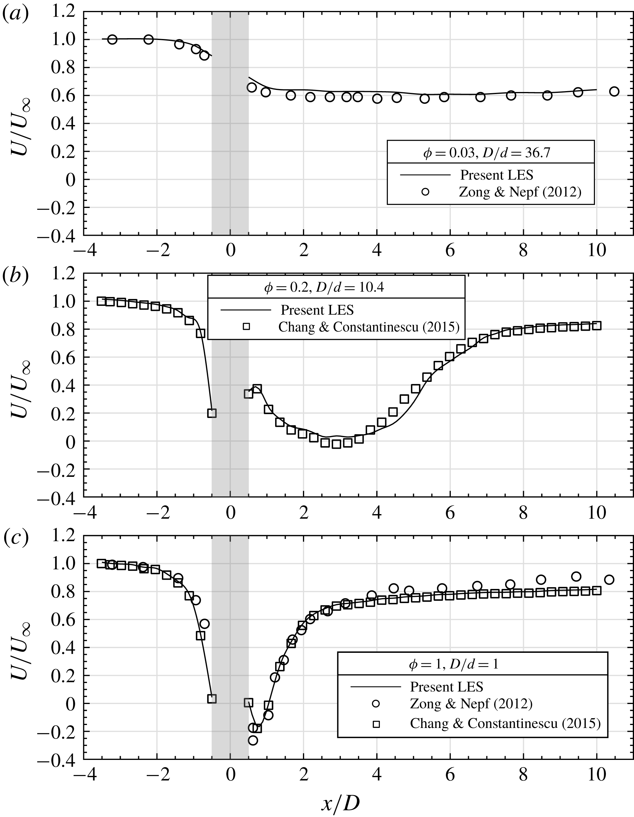
Secondly, simulations of flow impinging on an emergent cylindrical canopy patch having the same patch geometry (both the patch density,
 $\unicode[STIX]{x1D719}$
, and the separation of length scales,
 $D/d$
) as the experiments by Zong & Nepf (Reference Zong and Nepf2012) and the LES by Chang & Constantinescu (Reference Chang and Constantinescu2015) were conducted. Three patch densities are considered: relatively sparse (
 $\unicode[STIX]{x1D719}=0.03$
and
 $D/d=36.7$
), relatively dense (
 $\unicode[STIX]{x1D719}=0.2$
,
 $D/d=10.4$
), and a solid body (
 $\unicode[STIX]{x1D719}=1$
,
 $D/d=1$
). Consistent with existing studies on the downstream wake structure of an emergent canopy patch, figure 3 shows that, as
 $\unicode[STIX]{x1D719}$
increases, the steady wake region shortens and a faster recovery to the free-stream undisturbed condition is obtained. As can be seen from figure 3, the agreement between the present LES and experimental data is excellent.
2.3 Simulation set-up
The coordinate system and the numerical set-up are shown in figure 1(a), where
 $x$
is the streamwise direction,
 $y$
is the lateral direction and
 $z$
is the vertical direction. The time-averaged velocity components in the
 $x$
,
 $y$
and
 $z$
directions are denoted as
 $U$
,
 $V$
and
 $W$
, respectively. The origin of the coordinate system is located at the centre of the patch top surface. LES are conducted in a computational domain with dimensions of
 $54D\times 11D\times 36h$
(i.e. length
 $\times$
width
 $\times$
depth). The total depth is varied proportionally with the patch height,
 $h$
, to maintain a constant submergence ratio of
 $H/h=36$
, and the bottom boundary effect is neglected. A uniform incident velocity
 $U_{\infty }$
was prescribed at the inlet (
 $x=-L_{u}$
), and a convective boundary condition was used at the outlet (
 $x=L_{d}$
). The domain top boundary was modelled as a free-slip rigid lid that coincides with the patch top surface. All the solid surfaces were treated as no-slip walls.
As demonstrated in figure 1, a parametric study focusing on the effect of patch geometry under fixed flow forcing condition was performed, in which the patch density
 $\unicode[STIX]{x1D719}$
and aspect ratio
 $AR$
were varied independently. Following Nicolle & Eames (Reference Nicolle and Eames2011) and Taddei et al. (Reference Taddei, Manes and Ganapathisubramani2016), the cylinders were arranged in concentric circles with one cylinder at the centre of the canopy patch. The patch consists of
 $N_{c}$
individual solid cylinders of diameter
 $d=D/11$
, resulting in a patch density of
 $\unicode[STIX]{x1D719}=N_{c}(d/D)^{2}$
. All the LES runs were performed with
 $Re_{d}=U_{\infty }d/\unicode[STIX]{x1D708}=1000$
and
 $Re_{D}=U_{\infty }D/\unicode[STIX]{x1D708}=11\,000$
, which are considered to be representative of vegetation canopy patches in river flows (e.g. Leonard & Luther Reference Leonard and Luther1995; Zong & Nepf Reference Zong and Nepf2012).
Four patch densities
 $\unicode[STIX]{x1D719}$
were considered, including three porous patches plus a limiting case of a solid patch as shown in figure 1(b):
 $$\begin{eqnarray}\displaystyle \unicode[STIX]{x1D719}=0.16,~0.31,~0.50~\text{and}~1. & & \displaystyle\end{eqnarray}$$
For each value of
 $\unicode[STIX]{x1D719}$
,
 $h$
was varied to give four patch aspect ratios (
 $AR=h/D$
,
 $D$
was kept constant in this study) as:
 $$\begin{eqnarray}\displaystyle AR=0.25,~0.50,~0.75~\text{and}~1. & & \displaystyle\end{eqnarray}$$
This results in a total of 16 simulations. The same mesh resolution as used in the model validation in § 2.2 was used throughout the near-wake region. After the solution became statistically steady, time averaging was performed over an interval corresponding to approximately
 $20D/U_{\infty }$
.
3 General flow features
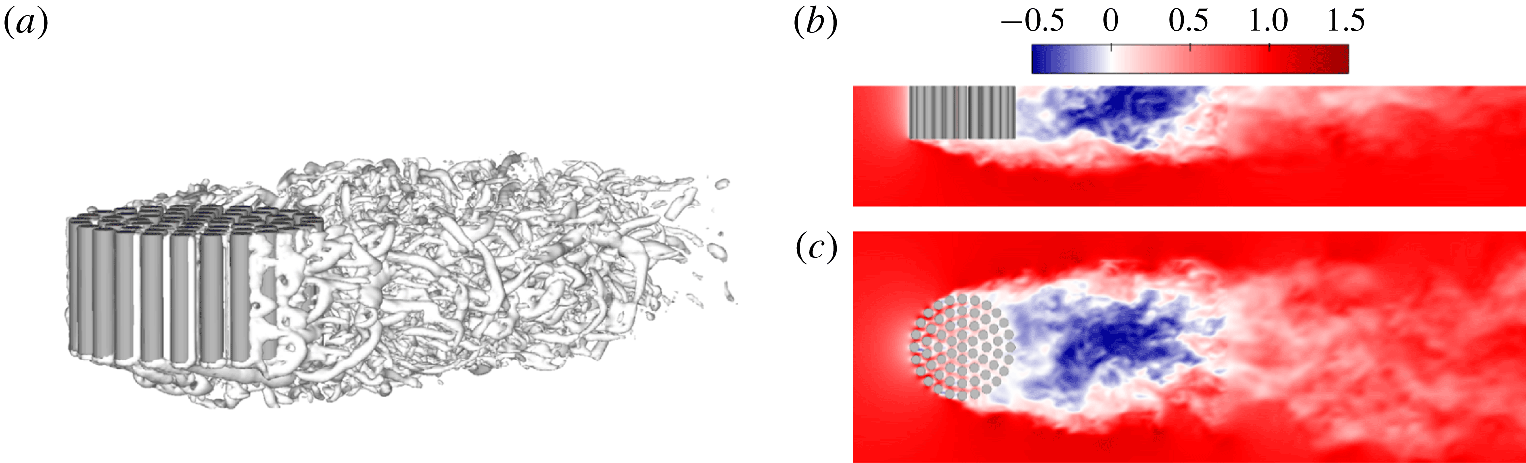
Instantaneous flow structures in the case
 $C_{61}AR_{0.50}$
. (a) Visualization of the vortex structures using the
 $Q$
-criterion. (b) Contours of
 $U_{inst}/U_{\infty }$
along the
 $x$
–
 $z$
plane at
 $y=0$
. (c) Contours of
 $U_{inst}/U_{\infty }$
along the
 $x$
–
 $y$
plane at
 $z=h/2$
. Here
 $U_{inst}$
denotes the instantaneous streamwise velocity.
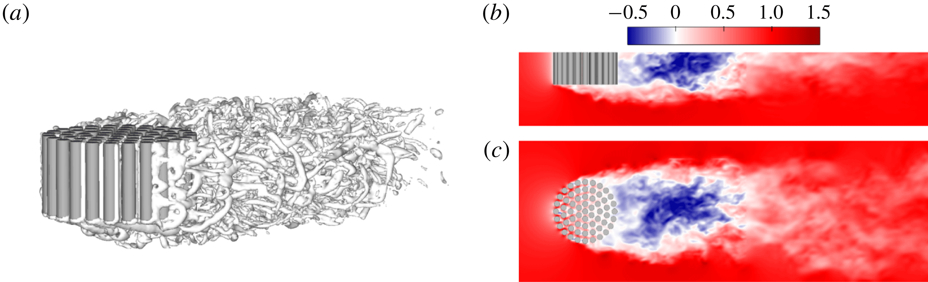
As an overview, we show the instantaneous downstream wake structure in figure 4 for the case
 $C_{61}AR_{0.50}$
(
 $\unicode[STIX]{x1D719}=0.50$
according to figure 1
b). Given the proximity between the downstream recirculation region and the trailing edge of the patch (similar to the case of a solid body), this can be considered as a relatively dense configuration (e.g. Nicolle & Eames Reference Nicolle and Eames2011; Taddei et al.
Reference Taddei, Manes and Ganapathisubramani2016). In the steady wake region, the separated shear layers (SSLs) at the lateral and bottom surface of the patch keep growing until they merge at some distance downstream, after which the flow starts to recover to the undisturbed condition. In figure 4(c), the wake signatures of the individual cylinders within the patch are annihilated due to strong wake interactions. For emergent canopies with sufficiently large canopy density (e.g.
 $\unicode[STIX]{x1D719}\geqslant 0.2$
in Chang & Constantinescu (Reference Chang and Constantinescu2015, their figure 7b)), the lateral SSLs become unstable some distance downstream and roll up into a patch-scale von Kármán vortex street. However, for the suspended patch considered here, the bottom SSL interferes with the interaction between the lateral SSLs and thus prevents the generation of a patch-scale vortex street. This is consistent with previous studies on the wake of a solid cylinder with a free end. As reviewed by Sumner (Reference Sumner2013), there exists a critical aspect ratio
 $AR_{c}$
below which the conventional von Kármán vortex street is completely suppressed by the interference of three-dimensional free-end flow. This critical aspect ratio appears to be sensitive to experimental conditions, and values of
 $AR_{c}=1{-}7$
can be found in the literature (e.g. Sakamoto & Arie Reference Sakamoto and Arie1983; Sumner, Heseltine & Dansereau Reference Sumner, Heseltine and Dansereau2004; Adaramola et al.
Reference Adaramola, Akinlade, Sumner, Bergstrom and Schenstead2006). Therefore, a patch aspect ratio of 0.50 as shown in figure 4, and actually all the values of
 $AR$
investigated in this paper (
 $0.25\leqslant AR\leqslant 1$
), are well below the minimum critical
 $AR$
beyond which the classical von Kármán vortex street would appear.
Effect of patch density on mean velocity fields in the near wake. Contours of (a,c)
 $U/U_{\infty }$
, (b)
 $W/U_{\infty }$
and (d)
 $V/U_{\infty }$
. From left to right, the columns show simulation cases with increasing
 $\unicode[STIX]{x1D719}$
while
 $AR$
is kept at 0.50.
Effect of patch aspect ratio on mean velocity fields in the near wake. Contours of (a,c)
 $U/U_{\infty }$
, (b)
 $W/U_{\infty }$
and (d)
 $V/U_{\infty }$
. From left to right, the columns show simulation cases with increasing
 $AR$
while
 $\unicode[STIX]{x1D719}$
is kept at 0.50 (
 $N_{c}=61$
).
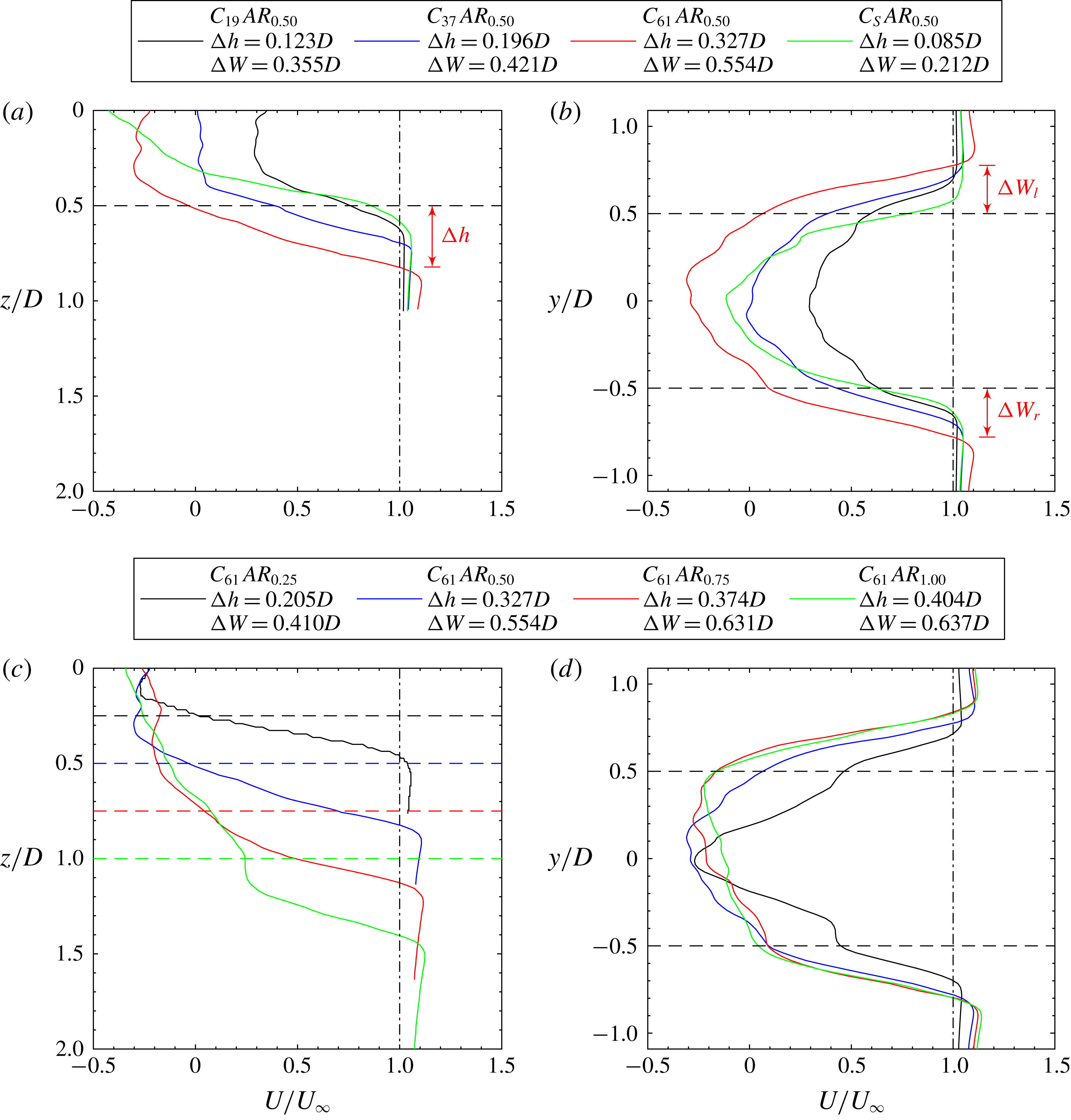
Quantification of the height (a,c) and width (b,d) of the near wake at
 $x=D$
in terms of profiles of mean streamwise velocity, corresponding to the cases shown in figures 5 and 6. The effect of
 $\unicode[STIX]{x1D719}$
is shown in (a,b) and the effect of
 $AR$
is shown in (c,d). Vertical and lateral profiles of
 $U/U_{\infty }$
are measured within the
 $x$
–
 $z$
plane at
 $y=0$
and the
 $x$
–
 $y$
plane at
 $z=h/2$
, respectively. In (a,c), the horizontal dashed line with the same colour as the
 $U/U_{\infty }$
profile depicts the respective vertical location of the patch free end (i.e.
 $z=h$
); while in (b,d) they mark the coordinates of the lateral extremities of the patch (i.e.
 $y=\pm D/2$
). The definition of wake enlargement with height
 $\unicode[STIX]{x0394}h$
and width
 $\unicode[STIX]{x0394}W=\unicode[STIX]{x0394}W_{l}+\unicode[STIX]{x0394}W_{r}$
is demonstrated for case
 $C_{61}AR_{0.5}$
.
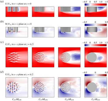
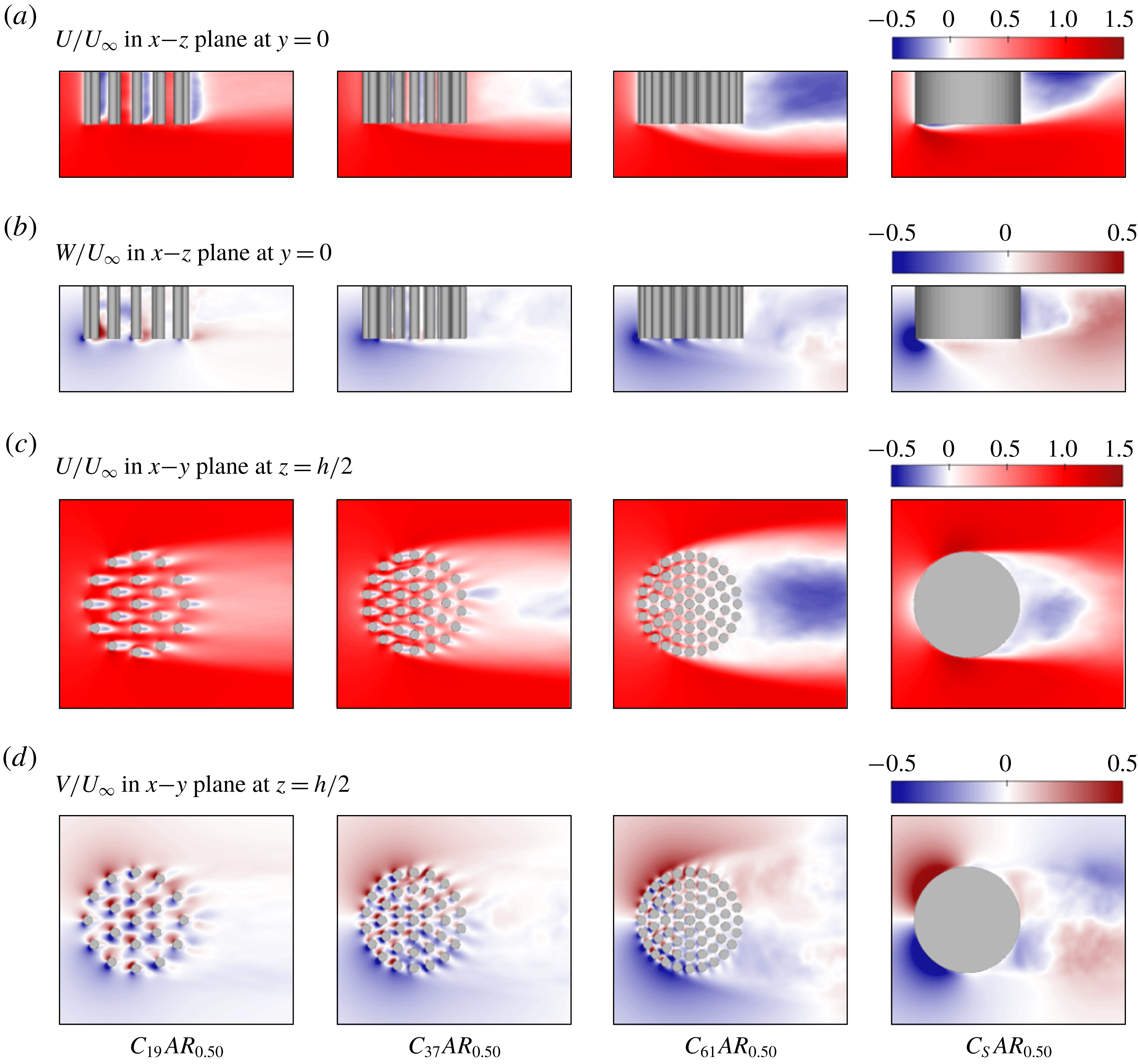
From here on, we focus on the mean-flow dynamics in the near field of the patch. Figure 5 shows the effect of canopy density on flow bleeding and the near-wake structure. For the porous patches (
 $\unicode[STIX]{x1D719}=0.16$
, 0.31 and 0.50), an increase in
 $\unicode[STIX]{x1D719}$
leads to weaker streamwise bleeding (figure 5
a,c) but stronger vertical bleeding (figure 5
b) and lateral bleeding (figure 5
d). As discovered in studies of emergent patches (e.g. Zong & Nepf Reference Zong and Nepf2012), the weakened streamwise bleeding contributes to shortening the total wake length over which the flow recovers to the free-stream velocity. However, this far-wake property is not further discussed in this paper.
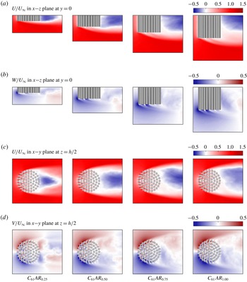
The effect of the bulk aspect ratio of the patch,
 $AR$
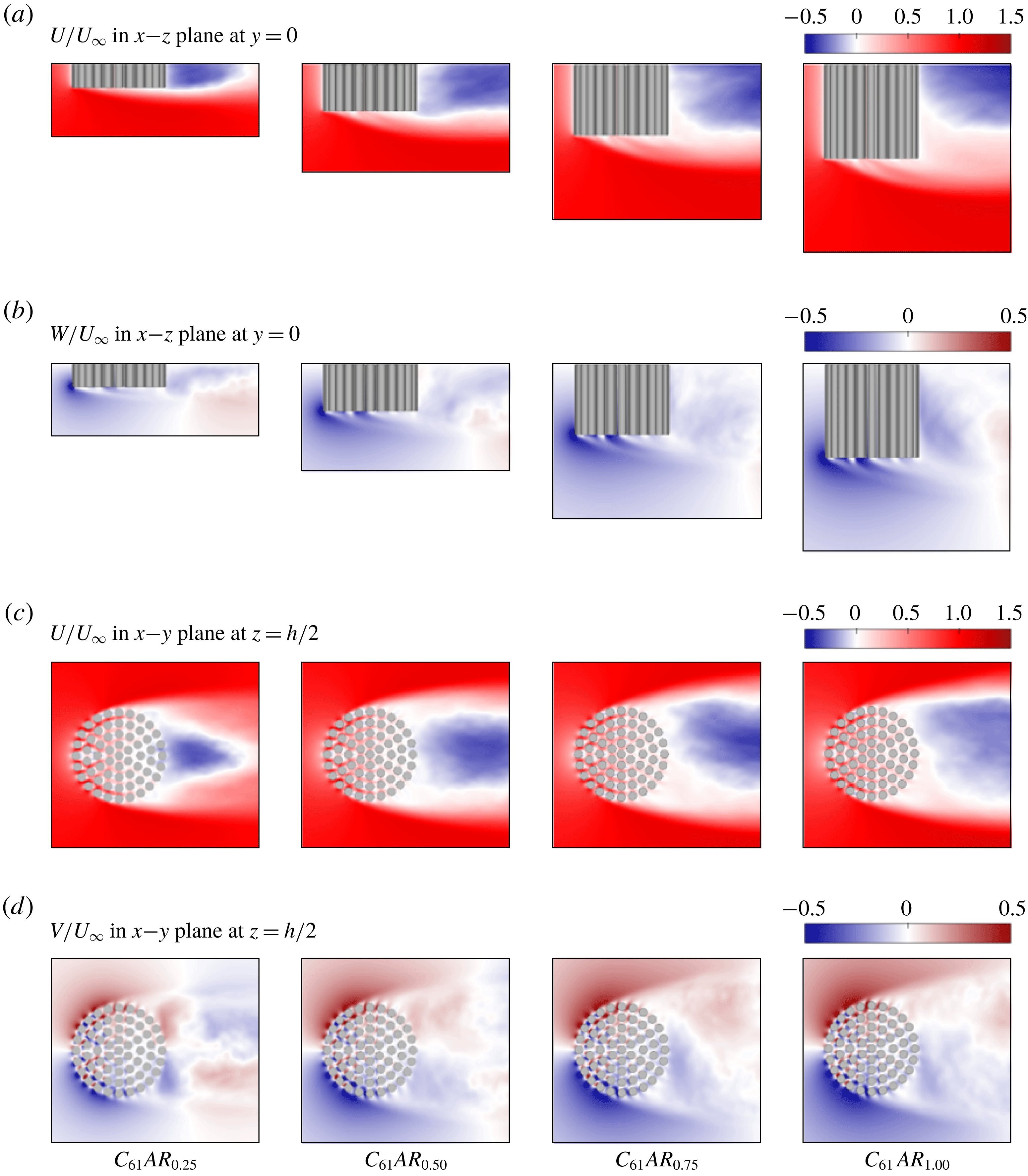
, on the near-wake structure is shown in figure 6, where it is found to be another important parameter that influences the flow bleeding dynamics of a finite canopy patch. In figure 6(b), the intensity of vertical bleeding from the patch bottom surface increases with increasing
 $AR$
, and the underlying mechanism will be illustrated in detail in § 4. Regarding the lateral bleeding, the magnitude of
 $V/U_{\infty }$
in figure 6(d) does not show a clear dependence on
 $AR$
. However, as
 $AR$
increases, regions with non-zero
 $V/U_{\infty }$
spread laterally, enlarging the width of the near wake.
Flow bleeding perpendicular to the incident flow tends to enlarge the effective height and width of the near wake as seen by the flow. It will be shown later that this ‘blowing up’ of the near wake has important implications for the global flow diversion (see § 6) and drag coefficients (see § 7) of a suspended canopy patch. Vertical bleeding perpendicular to the patch bottom surface pushes the bottom SSL downwards and thus enlarges the effective vertical size of the near wake (figures 5 a and 6 a). Similarly, the lateral bleeding pushes the lateral SSLs further to the sides and thus widens the near wake (figures 5 c and 6 c), despite the fact that the point of flow separation is fixed at the cylinders situated near the patch lateral extremities.
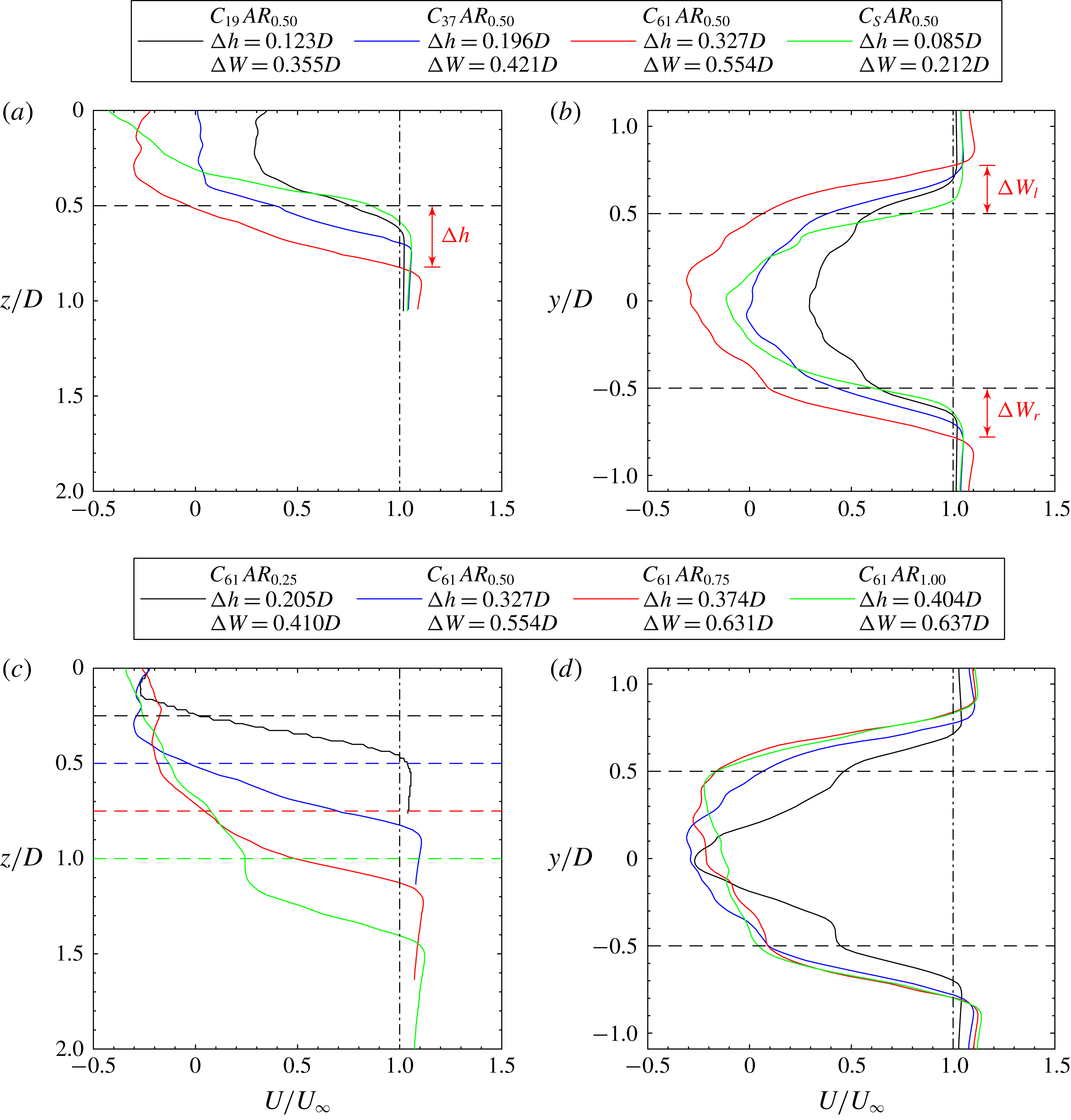
Figure 7 quantifies the dependence of wake enlargement at
 $x=D$
(i.e.
 $D/2$
downstream of the patch trailing edge) on the variation of
 $\unicode[STIX]{x1D719}$
and
 $AR$
. The effective height (
 $h_{e}$
) and width (
 $W_{e}$
) of the patch are defined respectively as
 $$\begin{eqnarray}\displaystyle h_{e}=h+\unicode[STIX]{x0394}h & & \displaystyle\end{eqnarray}$$
and
 $$\begin{eqnarray}\displaystyle W_{e}=D+\unicode[STIX]{x0394}W=D+\unicode[STIX]{x0394}W_{l}+\unicode[STIX]{x0394}W_{r}, & & \displaystyle\end{eqnarray}$$
where
 $h$
and
 $D$
are the actual height and width (or diameter) of the cylindrical patch,
 $\unicode[STIX]{x0394}h$
is the vertical distance between the patch bottom surface and the point where the mean streamwise velocity
 $U$
first recovers to the free-stream velocity
 $U_{\infty }$
, and
 $\unicode[STIX]{x0394}W_{l}$
(
 $\unicode[STIX]{x0394}W_{r}$
) is the lateral distance between the positive-
 $y$
(negative-
 $y$
) extremity of the patch and the point where
 $U$
first recovers to
 $U_{\infty }$
. The information embedded in figure 7 is consistent with the visualizations in figures 5 and 6. For porous patches (
 $\unicode[STIX]{x1D719}<1$
), increasing either
 $\unicode[STIX]{x1D719}$
or
 $AR$
leads to both larger
 $\unicode[STIX]{x0394}h$
and
 $\unicode[STIX]{x0394}W$
. There is a slower growth of the wake size at larger values of
 $AR$
due to the gradual transition to two-dimensional horizontal flow. For the solid patch (
 $\unicode[STIX]{x1D719}=1$
), the bleeding flows that promote wake enlargement and weaken wake entrainment are completely blocked, resulting in a wake region of the smallest dimensions compared with all the porous patches in both the spanwise (
 $y$
) and vertical (
 $z$
) directions.
4 Vertical motions inside the patch
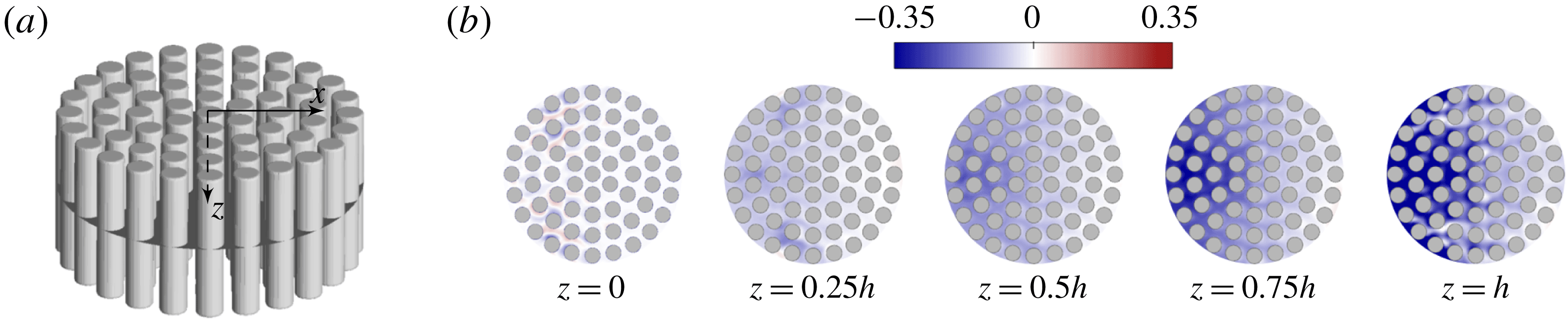
In this section, we provide a detailed look at the vertical motions inside the canopy patch. Figure 8 shows the pattern of vertical bleeding flows at different vertical levels along the height of the patch. Several important observations can be made: (i) Moving from the patch top boundary (
 $z=0$
) to its free end (
 $z=h$
), the overall intensity of vertical bleeding within the patch is enhanced. The explanation is that, as the patch free end is approached, there is a gradual transition from streamwise and/or lateral bleeding towards vertical bleeding, due to the shortened vertical distance needed to bleed out from the patch bottom surface. (ii) At a certain vertical level, vertical bleeding in the front half of the patch (
 $-D/2<x<0$
) is generally stronger than that in the rear half (
 $0<x<D/2$
). The reason for this behaviour is two-fold. Firstly, the total momentum of the incident flow decreases as it travels longitudinally through the patch interior, resulting in a gradually decreased amount of available momentum to be vertically diverted. Secondly, during the course of longitudinal advection, the flow gradually favours streamwise bleeding (or also lateral bleeding, depending on its
 $y$
location) with respect to vertical bleeding, because of the shortened horizontal distance needed to bleed out from the patch.
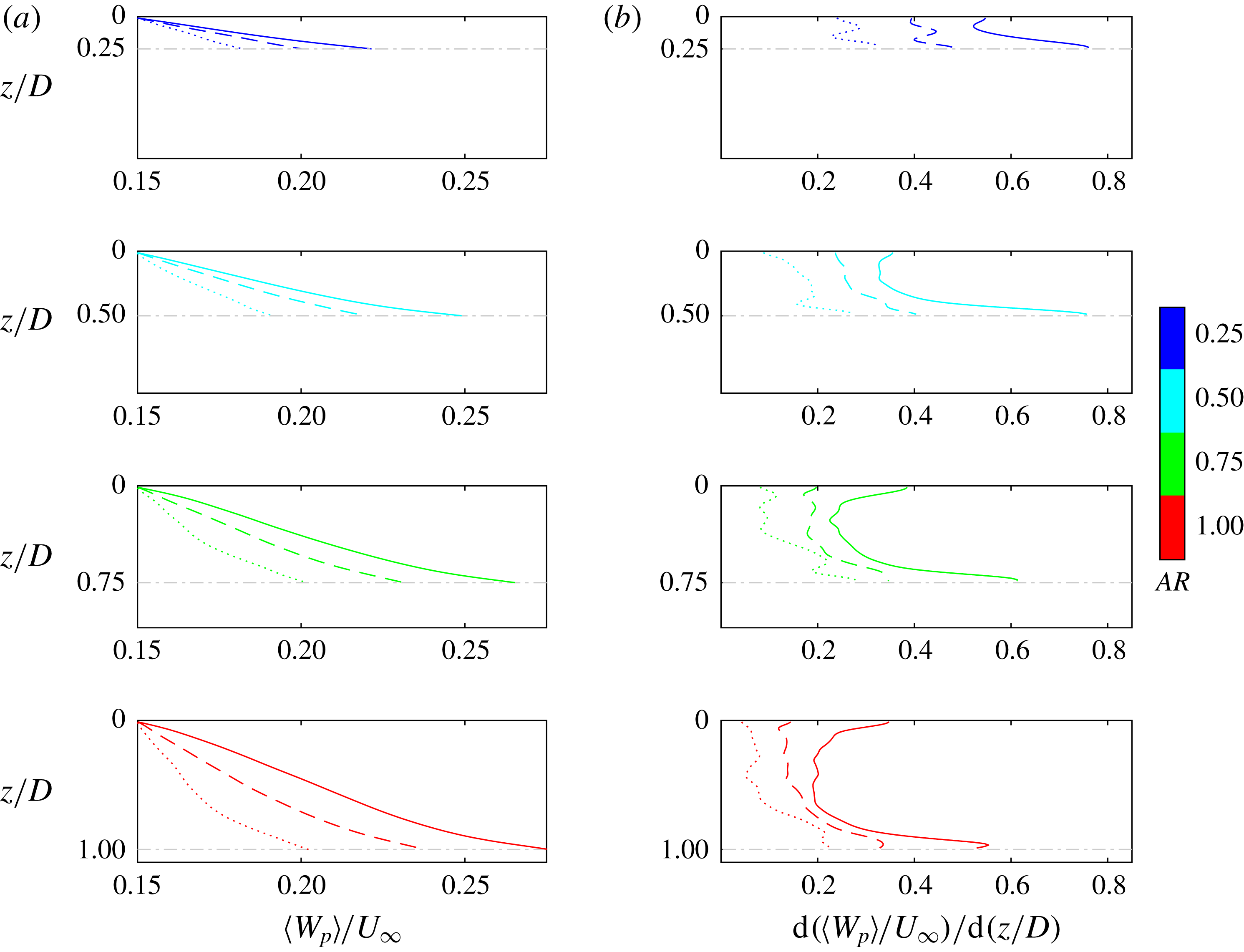
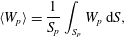
Quantification of the vertical bleeding as a function of the vertical coordinate is achieved as follows. In figure 8(a), starting from the patch top surface and downwards, the time-averaged vertical velocity field is horizontally averaged across the pore regions of the patch at every vertical level, i.e.
 $$\begin{eqnarray}\displaystyle \langle W_{p}\rangle =\frac{1}{S_{p}}\int _{S_{p}}W_{p}\,\text{d}S, & & \displaystyle\end{eqnarray}$$
where
 $S_{p}=(1-\unicode[STIX]{x1D719})(\unicode[STIX]{x03C0}D^{2}/4)$
is the plane area occupied by the pore regions,
 $W_{p}$
is the time-averaged vertical pore velocity, and
 $\text{d}S$
is the elemental area. The angle brackets indicate horizontal averaging.
For each simulation case with a specific
 $\unicode[STIX]{x1D719}$
–
 $AR$
combination, the general trend of variation of
 $\langle W_{p}\rangle$
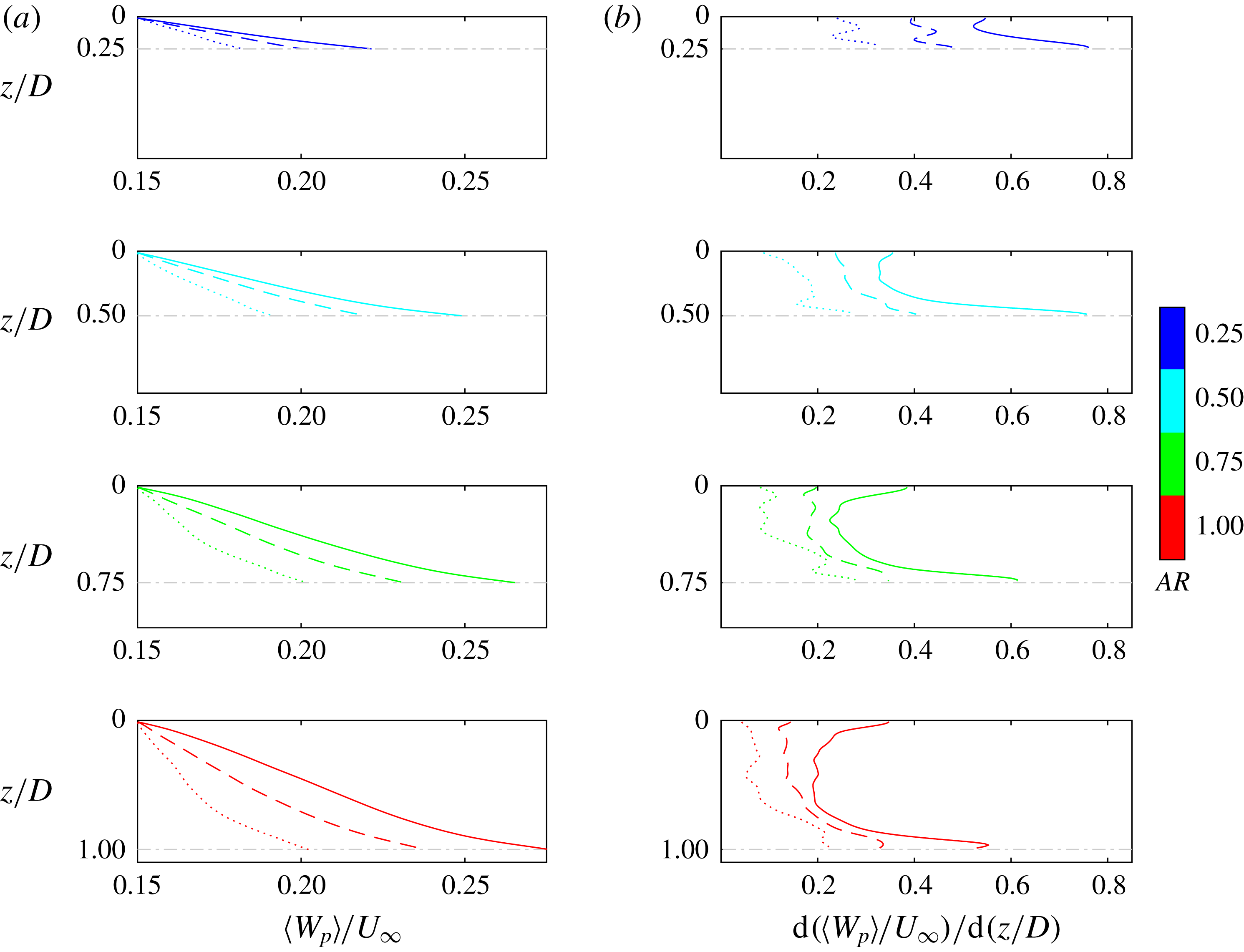
with
 $z$
in figure 9(a) is to be zero at the impermeable top surface and to increase monotonically towards the patch bottom surface. The vertical gradient of vertical bleeding velocity,
 $\text{d}(\langle W_{p}\rangle /U_{\infty })/\text{d}(z/D)$
, however, exhibits a non-monotonic variation with
 $z$
. On one hand, it is non-zero at
 $z=0$
due to the no-penetration boundary condition. On the other hand, at regions near the patch free end, there is a significant increase of
 $\text{d}(\langle W_{p}\rangle /U_{\infty })/\text{d}(z/D)$
. The underlying mechanism is that the abrupt expansion of cross-section below
 $z=h$
(depicted by the horizontal grey dash-dotted lines) promotes a rapid transition to vertical bleeding, i.e. the vertical pathway with the least drag that the flow has to experience before bleeding out of the patch. An intermediate region is observed where the vertical bleeding velocity is almost uniformly accelerating with respect to
 $z$
, i.e.
 $\text{d}(\langle W_{p}\rangle /U_{\infty })/\text{d}(z/D)$
is nearly constant with
 $z$
, except for the shortest patches with
 $AR=0.25$
.
(a) Zoom-in view of the vertically moving horizontal circular planes (dark grey) used for the visualization and spatial averaging of the vertical bleeding velocity within the pore regions. (b) Contours of
 $W_{p}/U_{\infty }$
at different vertical levels across the height of the patch. The simulation case shown is
 $C_{61}AR_{0.50}$
.
(a) Vertical profiles of
 $\langle W_{p}\rangle /U_{\infty }$
. (b) Vertical profiles of
 $\text{d}(\langle W_{p}\rangle /U_{\infty })/\text{d}(z/D)$
. In each plot, the horizontal grey dash-dotted line marks the location of patch bottom surface. The three patch densities are denoted respectively as
 $C_{19}$
(⋅ ⋅ ⋅ ⋅ ⋅),
 $C_{37}$
(– – –) and
 $C_{61}$
(——).
The non-dimensional vertical bleeding at the patch bottom surface can be expressed as
 $$\begin{eqnarray}\displaystyle \left.\frac{\langle W_{p}\rangle }{U_{\infty }}\right|_{z=h}=\int _{0}^{h/D=AR}\left[\frac{\text{d}(\langle W_{p}\rangle /U_{\infty })}{\text{d}(z/D)}\right]\,\text{d}(z/D). & & \displaystyle\end{eqnarray}$$
Note that the upper limit of integration,
 $h/D$
, amounts to the bulk aspect ratio of the patch. Based on (4.2), the observed dependences of the vertical bleeding on
 $\unicode[STIX]{x1D719}$
and
 $AR$
discussed in § 3 are interpreted as follows:
(i) When increasing
 $\unicode[STIX]{x1D719}$
with
$AR$
kept constant, since the cylinder arrangement is heavily staggered in the horizontal directions and aligned in the vertical direction as seen by the flow (figure 1), the increase of canopy resistance along the
$x$
- and
$y$
-directions is more prominent than along the
$z$
-direction. As a result, there is a tendency for the flow entering the patch to be vertically diverted as
$\unicode[STIX]{x1D719}$
increases. The end product is that in figure 9(b) a denser patch is accompanied by an overall faster acceleration of the vertical pore velocity with respect to
$z$
(i.e. larger
$\text{d}(\langle W_{p}\rangle /U_{\infty })/\text{d}(z/D)$
) over the same vertical distance of
$h$
(i.e. same
$AR$
), resulting in stronger vertical bleeding out of the patch bottom surface at
$z=h$
in figure 9(a). This is consistent with the velocity fields shown in figure 5(a,b) where stronger vertical bleeding pushes the bottom separated shear layer farther away from the patch free end of denser porous patches.
(ii) In figures 6(a,b) and 9(a), although increasing
$AR$
when keeping
$\unicode[STIX]{x1D719}$
constant also leads to stronger vertical bleeding at the patch bottom surface, the way it is achieved is different. Owing to the enlarged patch height as
$AR$
increases, the abrupt drag reduction at the patch bottom surface (
$z=h$
) has a weaker effect on promoting the transition from streamwise and/or lateral bleedings to vertical bleeding across the height of the patch, i.e. smaller overall
$\text{d}(\langle W_{p}\rangle /U_{\infty })/\text{d}(z/D)$
in figure 9(b) for taller patches. However, the flow entering the patch has to travel a longer vertical distance (i.e. non-dimensional height of the patch,
$h/D$
, in (4.2)) to bleed out from its bottom surface. In the end, the longer range of integration of the albeit smaller
$\text{d}(\langle W_{p}\rangle /U_{\infty })/\text{d}(z/D)$
results in a stronger vertical bleeding at the patch free end.








5 Local flow bleeding
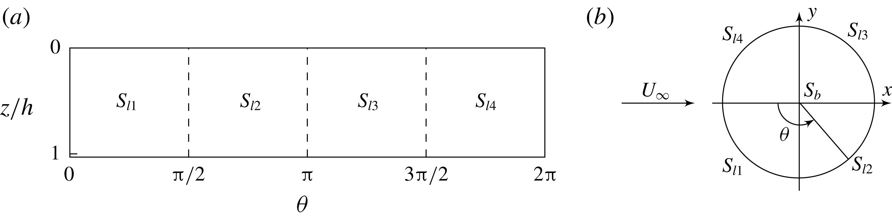
Based on the discussion in the preceding sections, we provide here a quantitative evaluation of the three-dimensional dynamics of flow bleeding of a cylindrical canopy patch that is separated from any boundary except for its top surface. The focus is on how the flow entering the patch is re-diverted along different directions in the form of bleeding, which corresponds to the local flow diversion described in § 1. A non-intrusive control volume closely following the patch outer surface shown in figure 10 was created, including its curved lateral surface (
 $S_{l1}$
,
 $S_{l2}$
,
 $S_{l3}$
,
 $S_{l4}$
) and a bottom surface (
 $S_{b}$
). The total inflow rate entering the patch is then expressed as
 $$\begin{eqnarray}\displaystyle Q_{inflow}=\left|\int _{S_{l1},S_{l4}}U\,\boldsymbol{i}\boldsymbol{\cdot }\boldsymbol{n}\,\text{d}S\right|. & & \displaystyle\end{eqnarray}$$
This must be equal to the total outflow rate leaving the patch surface,
 $$\begin{eqnarray}\displaystyle Q_{outflow}\equiv Q_{Bx}+Q_{By}+Q_{Bz}, & & \displaystyle\end{eqnarray}$$
where
 $$\begin{eqnarray}\displaystyle & \displaystyle Q_{Bx}=\left|\int _{S_{l2},S_{l3}}U\,\boldsymbol{i}\boldsymbol{\cdot }\boldsymbol{n}\,\text{d}S\right|, & \displaystyle\end{eqnarray}$$
 $$\begin{eqnarray}\displaystyle & \displaystyle Q_{By}=\left|\int _{S_{l1},S_{l2},S_{l3},S_{l4}}V\,\boldsymbol{j}\boldsymbol{\cdot }\boldsymbol{n}\,\text{d}S\right| & \displaystyle\end{eqnarray}$$
and
 $$\begin{eqnarray}\displaystyle Q_{Bz}=\left|\int _{S_{b}}W\,\boldsymbol{k}\boldsymbol{\cdot }\boldsymbol{n}\,\text{d}S\right| & & \displaystyle\end{eqnarray}$$
are referred to as the streamwise, lateral and vertical bleeding flow rates, respectively. In these expressions, the subscript
 $B$
indicates flow parameters evaluated along the patch outer surface (figure 10),
 $\text{d}S$
is the elemental area,
 $\boldsymbol{n}$
is the unit normal vector of the surface of the control volume and (
 $\boldsymbol{i},\boldsymbol{j},\boldsymbol{k}$
) are the unit vectors along the (
 $x,y,z$
) coordinates, respectively.
Sketch showing the surface of the control volume used to quantitatively evaluate the bleeding flow. (a) Lateral surface composed of four segments:
 $S_{l1}$
,
 $S_{l2}$
,
 $S_{l3}$
and
 $S_{l4}$
(laid flat). (b) Bottom surface (at
 $z/h=1$
). The origin of the
 $\unicode[STIX]{x1D703}$
-coordinate is located at the patch leading edge and is positive anticlockwise.

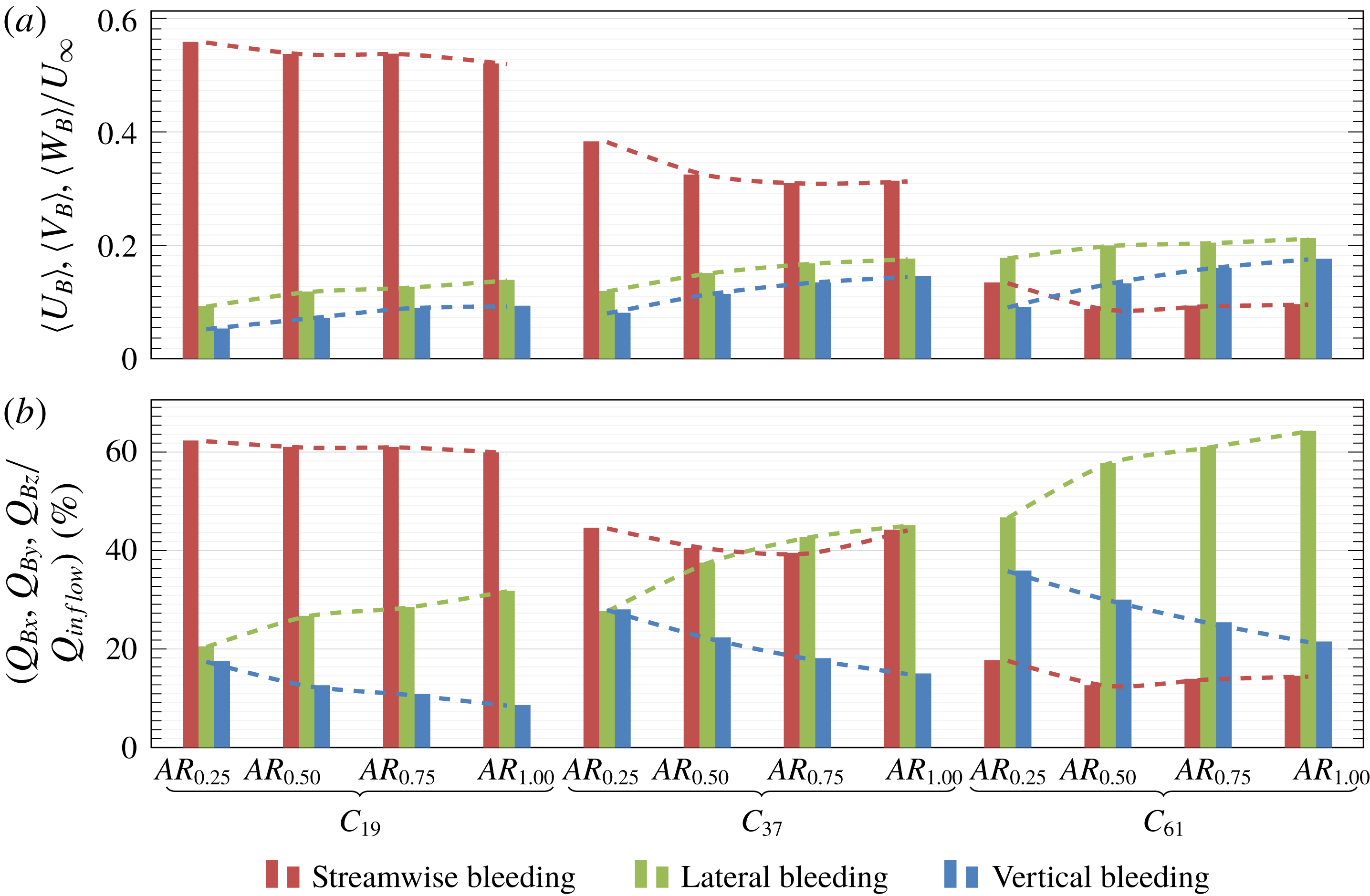
Three-dimensional bleeding dynamics through the control volume following the patch outer surface. (a) Bleeding velocities normalized by the free-stream velocity. (b) Proportion of bleeding flow rates relative to the total inflow rate. Dashed lines indicate the dependence of bleeding on
 $AR$
with
 $\unicode[STIX]{x1D719}$
being fixed.

Two aspects of the local flow bleeding are investigated here. Firstly, we define the ‘absolute bleeding’ as the intensities of the surface-averaged streamwise, lateral and vertical bleeding velocities normalized by the free-stream velocity:
 $$\begin{eqnarray}\displaystyle & \displaystyle \frac{\langle U_{B}\rangle }{U_{\infty }}=\frac{Q_{Bx}/(Dh)}{U_{\infty }}, & \displaystyle\end{eqnarray}$$
 $$\begin{eqnarray}\displaystyle & \displaystyle \frac{\langle V_{B}\rangle }{U_{\infty }}=\frac{Q_{By}/(2Dh)}{U_{\infty }}, & \displaystyle\end{eqnarray}$$
and
 $$\begin{eqnarray}\displaystyle \frac{\langle W_{B}\rangle }{U_{\infty }}=\frac{Q_{Bz}/(\unicode[STIX]{x03C0}D^{2}/4)}{U_{\infty }}. & & \displaystyle\end{eqnarray}$$
Secondly, the ‘relative bleeding’ is defined to be the redistribution of the flow rate entering the patch, manifested by the proportion of bleeding flow rates along different directions relative to the total inflow rate, i.e. a three-dimensional volumetric flux budget:
 $$\begin{eqnarray}\displaystyle Q_{Bx}/Q_{inflow}+Q_{By}/Q_{inflow}+Q_{Bz}/Q_{inflow}\equiv 1. & & \displaystyle\end{eqnarray}$$
Figure 11 gives an overview of the three-dimensional bleeding dynamics through the surface area of the 12 porous patches investigated in this paper. In terms of absolute bleeding (figure 11
a): (i) for a fixed
 $AR$
, as
 $\unicode[STIX]{x1D719}$
increases,
 $\langle U_{B}\rangle$
drops dramatically while
 $\langle V_{B}\rangle$
and
 $\langle W_{B}\rangle$
increase, consistent with the flow visualizations in figure 5; and (ii) for a fixed
 $\unicode[STIX]{x1D719}$
, larger values of
 $AR$
promote more horizontal flows inside the patch (because of weaker three-dimensional end effects across the patch height), leading to larger
 $\langle V_{B}\rangle$
. This confirms the discussion associated with figures 6 and 7 that more regions along the height of a taller patch are subject to strong lateral bleeding flows (i.e. less gain of
 $\unicode[STIX]{x0394}W$
at higher range of
 $AR$
in figure 7
d). As has been shown in § 3 and further analysed in § 4, the absolute vertical bleeding
 $\langle W_{B}\rangle$
increases with increasing
 $AR$
. To satisfy flow continuity, there is overall a slight decrease of
 $\langle U_{B}\rangle$
with increasing
 $AR$
.
Figure 11(b) demonstrates the dynamics of relative bleeding, i.e. the adjusted pathways of the flow entering the patch. The relative streamwise bleeding
 $Q_{Bx}/Q_{inflow}$
decreases significantly with increasing
 $\unicode[STIX]{x1D719}$
, and shows a weak dependence on
 $AR$
, similar to that of
 $\langle U_{B}\rangle$
. The increase of
 $Q_{By}/Q_{inflow}$
with both increasing
 $\unicode[STIX]{x1D719}$
and
 $AR$
is consistent with the discussions in § 3 (as large as 64 %), and it gradually exceeds
 $Q_{Bx}/Q_{inflow}$
at large values of
 $\unicode[STIX]{x1D719}$
or
 $AR$
. The effect of
 $AR$
on
 $Q_{By}/Q_{inflow}$
is two-fold. As previously mentioned, larger
 $AR$
promotes two-dimensional horizontal flows inside the patch and thus larger
 $\langle V_{B}\rangle$
. More importantly, it also indicates a larger lateral surface area of the cylindrical patch (
 $S_{l1-4}$
in figure 10) over which
 $\langle V_{B}\rangle$
is integrated in (5.4), while the area of the patch bottom surface stays unchanged as
 $AR$
varies. This results in a more significant increase of
 $Q_{By}/Q_{inflow}$
with increasing
 $AR$
than that of the surface-averaged
 $\langle V_{B}\rangle$
(compare the different slopes of the green dashed lines between figures 11
a and 11
b). The out-of-step variations of the patch lateral and bottom surface areas with
 $AR$
also lead to the most striking difference between figure 11(a) and (b) that
 $AR$
has opposite effects on
 $\langle W_{B}\rangle /U_{\infty }$
and
 $Q_{Bz}/Q_{inflow}$
. This reveals an important behaviour regarding the bleeding dynamics of a cylindrical canopy patch: as
 $AR$
increases, while stronger vertical bleeding velocity can be expected at the free end, a lower proportion of the total flow entering the patch interior is diverted vertically out of the patch.
6 Global flow diversion
In this section, we discuss the adjustment of the upstream undisturbed flow during its interaction with the suspended canopy patch, which is referred to as the global flow diversion in § 1. As depicted in figure 12(a), due to the canopy drag, the otherwise uniform total flow rate flushing through the whole computational domain,
 $Q_{\infty }=U_{\infty }BH$
, is redistributed into three pathways: penetrating through the patch (
 $Q_{t}$
), horizontally around the patch (
 $Q_{a}$
) and vertically beneath the patch (
 $Q_{b}$
), i.e.
 $$\begin{eqnarray}\displaystyle Q_{\infty }\equiv Q_{t}+Q_{a}+Q_{b}, & & \displaystyle\end{eqnarray}$$
if assuming fluid incompressibility. The change of flow rate in region
 $i$
(
 $i=t,a$
, or
 $b$
) with respect to the undisturbed condition is defined as
 $$\begin{eqnarray}\displaystyle \unicode[STIX]{x0394}Q_{i}=Q_{i}-Q_{i,\unicode[STIX]{x1D719}=0}, & & \displaystyle\end{eqnarray}$$
where
 $Q_{i,\unicode[STIX]{x1D719}=0}$
is the flow rate in region
 $i$
without the disturbances caused by the patch. It directly follows that
 $$\begin{eqnarray}\displaystyle |\unicode[STIX]{x0394}Q_{t}|\equiv |\unicode[STIX]{x0394}Q_{a}|+|\unicode[STIX]{x0394}Q_{b}|, & & \displaystyle\end{eqnarray}$$
because
 $Q_{t}$
always decreases while
 $Q_{a}$
and
 $Q_{b}$
always increase given the existence of a suspended canopy patch (Plew et al.
Reference Plew, Spigel, Stevens, Nokes and Davidson2006).
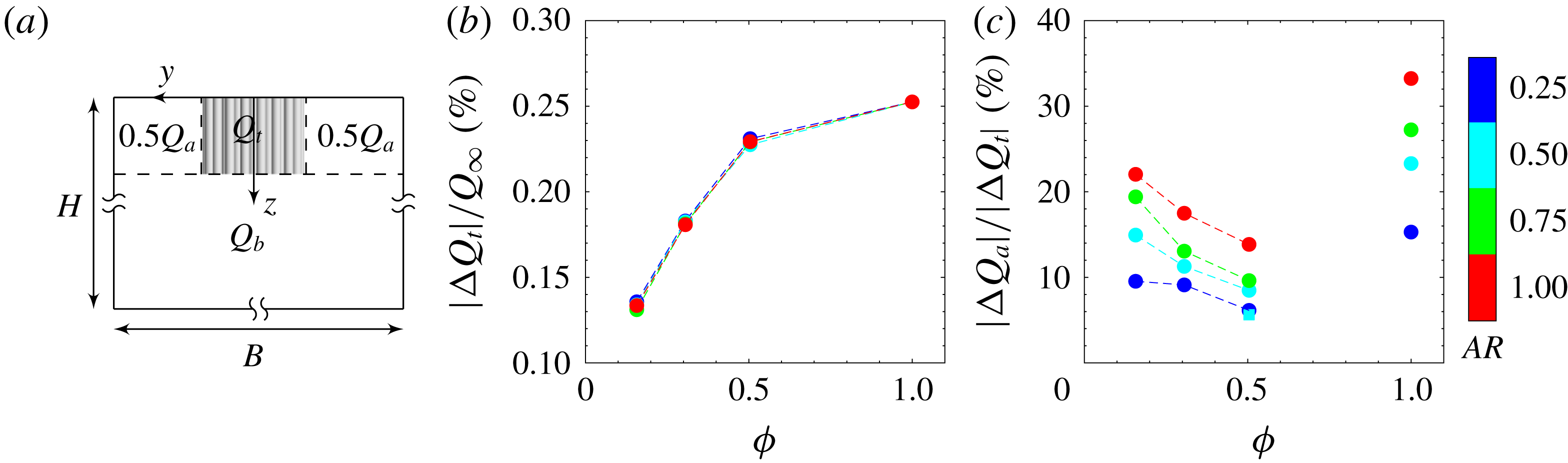
(a) Cross-sectional view at the
 $y$
–
 $z$
plane at
 $x=0$
showing the demarcations (dashed lines) between flow-through (
 $Q_{t}$
), flow-around (
 $Q_{a}$
) and flow-beneath (
 $Q_{b}$
) regions. (b) Effect of patch geometry on
 $|\unicode[STIX]{x0394}Q_{t}|$
normalized by
 $Q_{\infty }$
. (c) Effect of patch geometry on the proportion of
 $|\unicode[STIX]{x0394}Q_{a}|$
in
 $|\unicode[STIX]{x0394}Q_{t}|$
. The square pale blue symbol in (c) indicates the special case
 $C_{61}AR_{0.50}T$
where vertical bleeding is artificially blocked.

In what follows, we present the results of the proportional redistribution of the upstream undisturbed flow over the domain cross-section (i.e. global flow diversion) upon interaction with a canopy patch whose geometry varies in the
 $\unicode[STIX]{x1D719}$
–
 $AR$
parameter space. Moreover, an important observation from § 3 is that bleeding flows perpendicular to the main stream (i.e. local flow diversion) enlarge the size of the near wake, presenting to the flow as a wider (by lateral bleeding) or taller (by vertical bleeding) patch geometry than its actual dimensions. Taking the domain cross-section at
 $x=0$
as an example, the relationship between the global and local flow diversions is discussed as follows.
Figure 12(b) shows the reduction of flow rate through the patch interior normalized by
 $Q_{\infty }$
under the influence of varying patch geometry. It can be seen that
 $|\unicode[STIX]{x0394}Q_{t}|$
increases monotonically with patch densification and asymptotically approaches the solid-patch limit where
 $|\unicode[STIX]{x0394}Q_{t}|/Q_{\infty }=(Dh)/(BH)$
. Note that both
 $D/B$
and
 $h/H$
are kept the same across all the cases in this study, hence the curves with different values of
 $AR$
collapse. However, it is evident in figure 12(c) that partition of
 $|\unicode[STIX]{x0394}Q_{t}|$
into the flow-around and flow-beneath components (quantified by
 $|\unicode[STIX]{x0394}Q_{a}|/|\unicode[STIX]{x0394}Q_{t}|$
and thus
 $|\unicode[STIX]{x0394}Q_{b}|/|\unicode[STIX]{x0394}Q_{t}|=1-|\unicode[STIX]{x0394}Q_{a}|/|\unicode[STIX]{x0394}Q_{t}|$
) varies monotonically with
 $AR$
but possesses a non-monotonic dependence on
 $\unicode[STIX]{x1D719}$
. The explanation for such an anomalous dependence is provided next.
The patch density
 $\unicode[STIX]{x1D719}$
affects global flow diversion mainly by means of modifying local flow bleeding. The decrease of
 $|\unicode[STIX]{x0394}Q_{a}|/|\unicode[STIX]{x0394}Q_{t}|$
with increasing
 $\unicode[STIX]{x1D719}$
in figure 12(c) can be understood by considering the effect of local flow bleeding on the global flow diversion. In figures 5 and 7(a,b), as
 $\unicode[STIX]{x1D719}$
increases from 0.16 to 0.50, the effective height (3.1) and width (3.2) of the patch are increased due to vertical and lateral bleeding, respectively. In the mean time, when increasing
 $\unicode[STIX]{x1D719}$
at a fixed value of
 $AR$
in figure 11(b), a greater proportion of the flow entering the patch is locally diverted as lateral bleeding with respect to vertical bleeding (larger differences between
 $Q_{By}/Q_{inflow}$
and
 $Q_{Bz}/Q_{inflow}$
for denser patches). This growing dominance of lateral bleeding over vertical bleeding presents to the flow as a patch with smaller effective aspect ratio (
 $AR_{e}=h_{e}/W_{e}$
), hence promoting diversion of flow beneath the patch (i.e.
 $|\unicode[STIX]{x0394}Q_{a}|/|\unicode[STIX]{x0394}Q_{t}|$
decreases with increasing
 $\unicode[STIX]{x1D719}$
). To verify this statement, an additional simulation
 $C_{61}AR_{0.50}T$
was carried out, where a circular thin plate of diameter
 $D$
is attached to the patch bottom surface to eliminate vertical bleeding and presumably enhance lateral bleeding. As expected,
 $|\unicode[STIX]{x0394}Q_{a}|/|\unicode[STIX]{x0394}Q_{t}|$
drops from
 $8.5\,\%$
to
 $5.6\,\%$
in figure 12(c).
In figure 12(c), the value of
 $|\unicode[STIX]{x0394}Q_{a}|/|\unicode[STIX]{x0394}Q_{t}|$
associated with the limiting case of a solid patch (
 $\unicode[STIX]{x1D719}=1$
) turns out to be larger compared with all the porous patches with the same aspect ratio. The reason is that, for all the cases in figure 11(b), the relative lateral bleeding is stronger than the relative vertical bleeding, which indicates that the canopy porosity promotes flow diversion beneath the patch (i.e. smaller
 $|\unicode[STIX]{x0394}Q_{a}|/|\unicode[STIX]{x0394}Q_{t}|$
compared to the solid patch with no bleeding flows). Given the monotonically varying flow dynamics of the porous patches with different
 $\unicode[STIX]{x1D719}$
investigated in this study, there clearly exists a turning point between
 $\unicode[STIX]{x1D719}=0.50$
and
 $1$
after which bleeding along all directions starts to recede with increasing
 $\unicode[STIX]{x1D719}$
. The corresponding uncertainty of the flow dynamics precludes a monotonic interpolation over the range of
 $\unicode[STIX]{x1D719}=0.50{-}1$
in figure 12(c). This is beyond the scope of the current study and we leave it as a subject for future work.
The patch aspect ratio
 $AR$
affects global flow diversion by changing the relative dimensions of the patch between the vertical and lateral directions. For patches with larger
 $AR$
, the three-dimensional disturbances induced by the patch free end are weaker across the patch height; therefore the flow adjustment is less three-dimensional and favours a lateral diversion around the patch other than vertical diversion, i.e.
 $|\unicode[STIX]{x0394}Q_{a}|/|\unicode[STIX]{x0394}Q_{t}|$
increases with increasing
 $AR$
in figure 12(c). Regarding the size of the near wake, a growing dominance of lateral bleeding over vertical bleeding as
 $AR$
increases can be observed in figure 11(b), which tends to promote vertical diversion beneath the patch. However, it cannot counteract the promotion of lateral diversion around taller patches as
 $AR$
increases.
7 Drag coefficients
The time-averaged bulk drag coefficient of the canopy patch is defined by
 $$\begin{eqnarray}\displaystyle C_{D}=\frac{F_{D}}{0.5\unicode[STIX]{x1D70C}U_{\infty }^{2}Dh}, & & \displaystyle\end{eqnarray}$$
where
 $F_{D}$
is the total time-averaged drag force exerted on the patch,
 $\unicode[STIX]{x1D70C}$
is the fluid density, and
 $D$
and
 $h$
are the diameter and height of the cylindrical patch, respectively. From a momentum balance point of view, the value of
 $C_{D}$
is mainly influenced by the spread of its wake and the intensity of the velocity deficit in the wake itself. For porous patches, there are mainly four flow phenomena that affect the drag coefficient compared with their solid counterparts with the same bulk dimensions (Nicolle & Eames Reference Nicolle and Eames2011; Chang & Constantinescu Reference Chang and Constantinescu2015; Taddei et al.
Reference Taddei, Manes and Ganapathisubramani2016): (i) the internal cylinders offer some extra resistance to the incident flow, i.e. larger
 $C_{D}$
; (ii) the streamwise bleeding contributes to diminishing the velocity deficit in the wake and hence to lower
 $C_{D}$
; (iii) the lateral bleeding prevents the reattachment of the flow along the sides of the porous patches, hence contributing to widening the wake, i.e. larger
 $C_{D}$
; and (iv) the vertical bleeding pushes downwards the shear layer forming at the patch bottom, hence enlarging the vertical size the wake, i.e. larger
 $C_{D}$
.
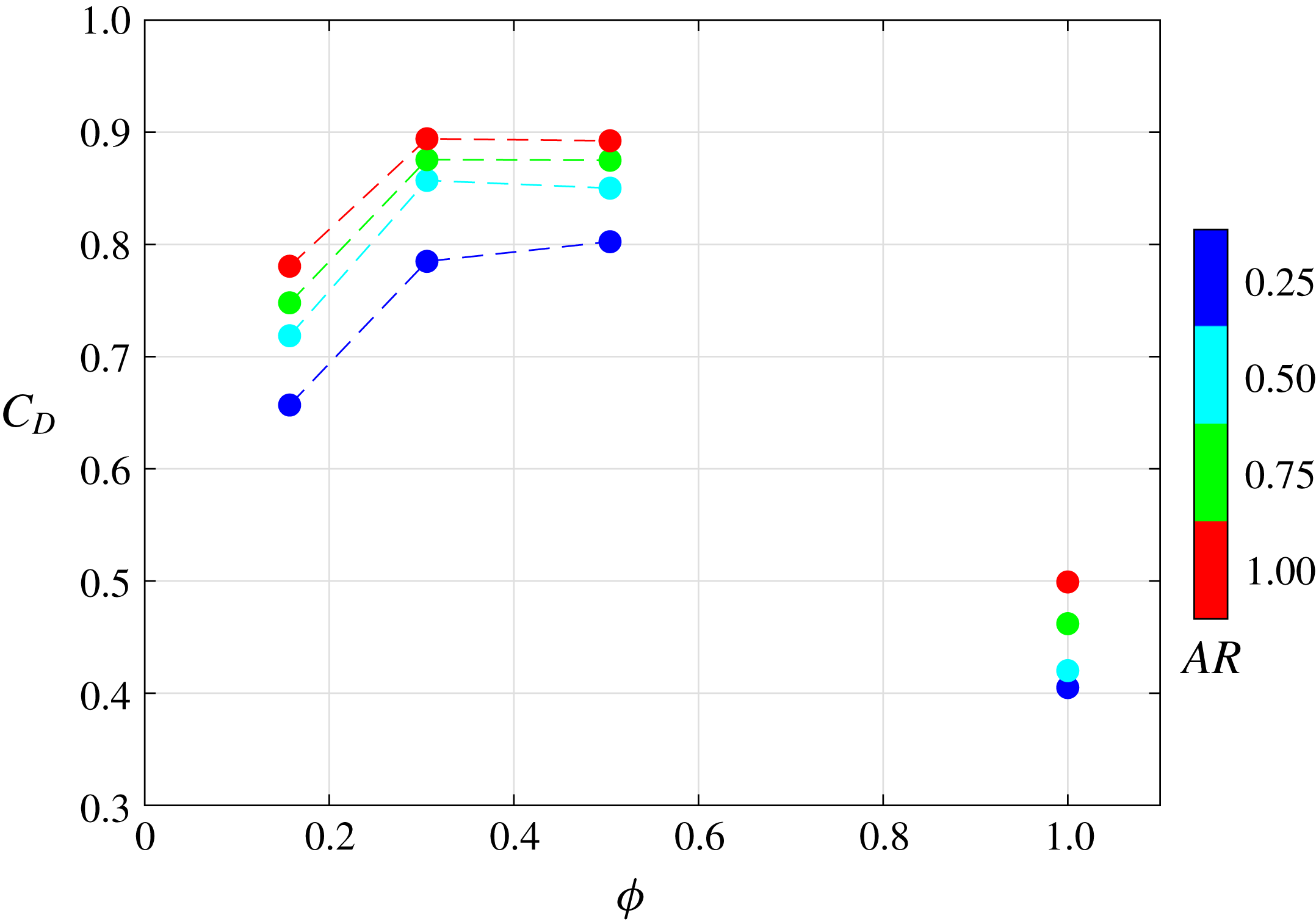
Time-averaged drag coefficient versus patch density and aspect ratio.

Figure 13 shows the effects of patch density and aspect ratio on the time-averaged drag coefficient of the patch. For a fixed
 $AR$
,
 $C_{D}$
increases as
 $\unicode[STIX]{x1D719}$
increases from 0.16 to 0.31, and reaches a plateau between
 $\unicode[STIX]{x1D719}=0.31$
and 0.50. During this process, the increase of the number of constituent cylinders, the decrease of streamwise bleeding and increase of lateral/vertical bleeding as shown in figure 11(a) all contribute to increasing
 $C_{D}$
. However,
 $C_{D}$
drops abruptly for the solid patch (
 $\unicode[STIX]{x1D719}=1$
), which is almost half of the maximum value observed for the porous patches. For example, the ratio between the minimum and maximum
 $C_{D}$
(from case
 $C_{S}AR_{1.00}$
and
 $C_{37}AR_{1.00}$
, respectively) is 56 %, which is identical to the value reported by the experiments of Taddei et al. (Reference Taddei, Manes and Ganapathisubramani2016). This can be attributed to the absence of internal resistance from the individual cylinders as well as the vertical and lateral bleeding flows that enlarge the near wake. The more intensive velocity deficit in the wake of the solid patch due to the zero streamwise bleeding cannot counteract all these effects, making the
 $C_{D}$
of the solid patch even smaller than the sparsest case with
 $\unicode[STIX]{x1D719}=0.16$
. Similar to figure 12(c), there is a big gap of data between
 $0.50<\unicode[STIX]{x1D719}<1$
over which the flow property is uncertain. Therefore, a monotonic interpolation is also not made within this range.
By contrast, the variation of
 $C_{D}$
with
 $AR$
is monotonic. It can be seen that the values of
 $C_{D}$
of patches with a larger
 $AR$
are generally larger, and the reason is two-fold. Firstly, if only considering the external dimensions of the patch (
 $h$
and
 $D$
), the bottom shear layer, which induces wake entrainment and hence decreases the pressure drag, is weaker for taller patches, which has been confirmed by previous studies of a circular cylinder with a finite height (e.g. Inoue & Sakuragi Reference Inoue and Sakuragi2008). Secondly, taking the canopy porosity into consideration, an increase in
 $AR$
promotes vertical and lateral bleedings while inhibiting streamwise bleeding (see figure 11
a). All these effects contribute to increasing
 $C_{D}$
, with no counteractive mechanisms.
8 Conclusions
In this paper, large-eddy simulations were conducted to study the mean flow dynamics in close vicinity of a cylindrical canopy patch. A deep-water condition is prescribed to eliminate the effect of varying submergence ratio
 $h/H$
, while we provide a systematic investigation of the flow response in the
 $\unicode[STIX]{x1D719}$
–
 $AR$
parameter space, where
 $\unicode[STIX]{x1D719}$
is the canopy density and
 $AR=h/D$
is the bulk aspect ratio. It was highlighted for the first time that, apart from
 $h/H$
and
 $\unicode[STIX]{x1D719}$
, the patch aspect ratio plays an important role in determining the near-wake structure of a suspended canopy patch with finite length and width.
The local three-dimensional flow bleeding dynamics was analysed in detail. The streamwise/lateral/vertical bleeding velocities (i.e. absolute flow bleeding) decreases/increases/increases with both increasing
 $\unicode[STIX]{x1D719}$
and
 $AR$
. Through a volumetric flux budget, the proportion of bleeding flow rates along different directions relative to the total flow rate entering the patch (i.e. relative flow bleeding) shows similar parametric dependences. The exception is that a larger
 $AR$
causes a smaller proportion of the total flow entering the patch to bleed out vertically, due to the enlarged lateral surface area of the patch.
The global flow diversion (i.e. redistribution of upstream undisturbed flow into pathways through, around and beneath the patch) is determined by the actual geometry of the patch as well as the spread of its wake. Taller patches with larger
 $AR$
promote an overall stronger lateral diversion because of the weakened end effect across the patch height. When it comes to the effect of varying
 $\unicode[STIX]{x1D719}$
, although the external geometric dimensions (i.e.
 $h$
and
 $D$
) of the patch stay unchanged, local flow bleeding modifies the global flow diversion. Bleeding flows perpendicular to the incident flow push the separated shear layers farther away from the patch and thus enlarge the effective height and width of the near wake. A larger proportion of the flow entering the patch is diverted laterally as
 $\unicode[STIX]{x1D719}$
increases, presenting to the flow as a patch with smaller effective aspect ratio, which promotes stronger vertical diversion beneath the patch. In a multi-patch system, this redistribution of upstream streamwise flow is expected to influence the flow condition of adjacent patches and thus the overall functioning of the system.
The flow responses of porous patches and their solid counterparts (
 $\unicode[STIX]{x1D719}=1$
) are fundamentally different, as manifested by the sizes of the near wake, the global flow diversion and the bulk drag coefficients. This is attributed to the absence of bleeding flows in the solid patch. In this study, it is impossible to construct patches with
 $\unicode[STIX]{x1D719}>0.50$
while maintaining a constant value of
 $D/d=11$
. The lack of data between
 $\unicode[STIX]{x1D719}=0.50$
and
 $1$
calls for additional work investigating the transition of flow dynamics between dense patches (e.g.
 $\unicode[STIX]{x1D719}=0.50$
) and a solid body with the same external dimensions.
It is noteworthy that suspended canopies cannot be simply viewed as inverted submerged canopies. The major difference between suspended and submerged canopies is the influence of the bottom boundary layer. In submerged canopies, except for highly porous scenarios, bottom friction has been found to play a secondary role in velocity profiles due to the dominating canopy drag (Plew Reference Plew2011; Zong & Nepf Reference Zong and Nepf2012; Chang & Constantinescu Reference Chang and Constantinescu2015). For suspended canopies in shallow water, bottom friction tends to have a significant influence on the undercurrent through the gap between canopy and the bottom boundary. However, in deep water, the effect of bottom boundary layer on suspended canopies can be largely neglected due to the large gap in between. In this case, the flow associated with bottom-mounted and surface-suspended canopies are expected to behave in a similar manner, and the difference diminishes with increasing canopy density.
As a final comment, the present study serves as a first step towards a better understanding of flow interacting with a suspended canopy patch. Hence, we note that future studies with increasing complexity need to be conducted. For example, the shape and flexibility of the internal elements as well as the ratio of
 $D/d$
are likely to change the canopy drag characteristics. Additionally, for canopy patches suspended in shallow water, the proximity of the bottom boundary and the resulting accelerating undercurrent are likely to modify the aforementioned three-dimensional flow dynamics in deep water.
Acknowledgements
The authors are grateful to the anonymous referees for their constructive comments and recommendations. We gratefully acknowledge the support of both the Office of Naval Research under grant no. N00014-16-1-3015 (Scientific Officers: Dr T. Paluszkiewicz and Dr S. Harper) and the National Science Foundation under CAREER grant OCE-1151838.