Introduction
As a versatile approach, adaptive beamforming (ABF) has received considerable attentions over the past several decades and became a fundamental technique for numerous applications including radio astronomy, applied acoustic, cognitive communications, and medical imaging[Reference Komljenovic, Helkey, Coldren and bowers1–Reference Bing and Leger3]. ABF possesses the potential to optimize the radiation pattern in real-time, which obtained a larger output signal-to-interference-plus-noise ratio (SINR) by steering the main lobe of radiation toward a desired signal while placing respective nulls toward several interference signals [Reference Zaharis, Skeberis, Xenos, Lazaridis and Cosmas4].
Classic ABF techniques used to extract the respective array excitation weights are based on two main criteria: minimum mean square error (MMSE) and maximum signal-to-noise ratio (MSINR) [Reference El-Keyi and Champagne5, Reference Hassani, Plata-Chaves, Bertrand and Moonen6]. Representative ABF algorithm is the minimum variance distortionless response (MVDR) on the basis of MSINR criterion. Although this method is capable of suppressing the interference and improving system reliability, weights computed by MVDR are not able to form the deep nulls toward the interference source in various interference scenarios on account of the characteristics of this technique. Conventional methods to solve this problem are very time consuming and are unmanageable in ABF application. Another criterion for computing the array weights is to minimize the MMSE, one of the most widely used MMSE-based adaptive algorithms is least mean square approach, this method needs a training sequence of signal of interest to adjust the complex weights adaptively and minimize the difference between the array output for forming the optimum array pattern [Reference Roshanaei, Lucas and Mehrabian7, Reference Al-Ardi, Shubair and Al-Mualla8]. However, it exhibits a high probability of tracking into local optimal solution, which may not be applicable for ABF in harsh environments. Consequently, the inherent shortcomings of the derivative-based ABF methods have compelled and motivated many researchers to explore meta-heuristics (MH) and evolutionary methods for overcoming these types of difficulties [Reference Rasmussen and Krink9].
The main advantage of the evolutionary heuristics algorithms over the classical derived approaches is their ability to search the global optimum of the objective functions without using the derivatives of the objective functions. In addition, MH optimization algorithms have no requirements for extra iterative derivations or computationally extensive routines of ABF with objective functions. According to the above, an enormous amount of evolutionary algorithms has been dedicated to applying several optimization approaches for ABF problems in the past decades. Many literatures have shown that these algorithms are capable of finding global or strong local optima of non-linear multimodal functions with multidimensional solutions [Reference Wei and Lu10, Reference Vitale, Vesentini, Ahmad and Hanzo11]; therefore, weights of the beamformer extracted by the optimization techniques according to the fitness function defined by specific criterion can be used to place a maximum beam and null in an array pattern in specified locations. Compared to other evolutionary algorithms, the PSO is much easier to implement and outperform better; thus, many examples have been successfully demonstrated and validated the design flexibility of PSO in the framework of ABF arrays [Reference Maina, Langat and Kihato12–Reference Mahmoud, El-Adawy, Ibrahem, Bansal, Mahmoud and Zainud-Deen14].
Although the MH-based ABF algorithm requires relatively lower mathematical complexity than derivative-based or iterative-based ABF methods, there still exist the weaknesses and limitations in the application of ABF. Some optimization algorithms are highly dependent on starting points in the case of a large number of solution variables, yet the weights of ABF are regularly associated with a large number of array elements, and the excitation of array elements is complex, i.e. having both amplitude and phase, hence the ABF solution space cannot be very small, in that case, the conventional evolutionary algorithm is not really applicable to ABF. Besides, the classic optimization methods are prone to get trapped in local minima and not reach the global optimum [Reference He and Huang15] when solving complex multimodal optimization problems of array weight extraction, resulting in a suboptimum beamforming performance. In addition, most of MH algorithms are population-based optimization techniques which require long execution times to converge, specifically when solving large-scale complex ABF engineering problems [Reference Berryman, Allison and Abbott16, Reference Korošec, Šilc and Filipič17], and the complexity implementing the algorithms would also result in huge cost and hardware resources.
In consideration of the above-mentioned studies, we propose a novel interactive-based random iterative search strategy, called Fibonacci branch search (FBS) in this paper to deal with complicated optimization problems of ABF. The concept of the proposed FBS is defined from two aspects: The first one is the generation principle of Fibonacci branch architecture. The establishment of branch structure in FBS is built up on the optimization process of the searching points, and the shortening fraction is designed based on Fibonacci sequence for the generation of a set of optimization elements that consist of two types of searching points. The optimization endpoints search for the optimal solution according to the growth path mode of the branch. The second standpoint of the FBS concept is the construction of the interaction iteration that applies rules for the computation of the optimization elements. The iterative rules are composed of global searching and local optimization, which are the two phases necessary to update the optimization elements. Global tentative points and local searching points are formulated in the phase of two interaction processes, and the points with the best fitness converge toward the global optimum in searching space. At the same time, computer memory can be fully used to record the optimizing process during the interaction optimization course. Global randomness is one of the important characteristics of FBS, and this mechanism is implemented on those points that do not readily fall into the local optimum and are not able to find a better solution.
The novelty of this paper lies in the fact that we design the Fibonacci branch optimization structure and propose the novel global searching and local optimizing interaction iterative technique. In addition, the FBS algorithm proposed here has been applied to antenna array beamforming in several cases and in comparison with other evolutionary optimization-based techniques on several test functions and the robust ABF. To the best of our knowledge, the proposed novel FBS optimization algorithm has been applied for the first time in antenna array beamforming problems.
The reminder of this paper is organized as follows: ABF system model of ULA is described in section “ABF system model of ULA and problem statement”. Section “Proposed FBS algorithm” presents the proposed FBS optimization algorithm. Later, section “FBS-based beamformer design and implementation of ABF with the proposed FBS” introduces the robust ABF based on FBS. The validation of the proposed FBS via benchmark functions and the simulation results are reported in section “Simulation results”. Section “Conclusions” gives the conclusion.
ABF system model of ULA and problem statement
Consider a uniform linear antenna array of M omni-directional array elements employed in ABF receiver, one desired signal and Q uncorrelated interferences which impinge on the array at  $k$th snapshot can be expressed by [Reference Liao and Chan18]
 $${\bf x}\lpar k \rpar = s\lpar k \rpar {\bf a}\lpar {\theta_d} \rpar + \sum\limits_{i = 1}^Q {i_i\lpar k \rpar {\bf a}\lpar {\theta_i} \rpar } + {\bf n}\lpar k \rpar \comma \;$$
where  $s\lpar k \rpar $ and
 $i_i\lpar k \rpar $ are the desired GNSS signal and the
 $i{\rm th}$ interference,
 ${\bf n}\lpar k \rpar $ denotes the complex vector of sensor noise.
 ${\bf a}\lpar {\theta_d} \rpar $ and
 ${\bf a}\lpar {\theta_i} \rpar $ represent
 $M \times 1$ steering vectors of
 $s\lpar k \rpar $ and
 $i_i\lpar k \rpar $ as given by
 $$\eqalign{& {\bf a}\lpar {\theta_d} \rpar {\rm}= \lsqb {1{\rm \comma \;}{\rm e}^{{-}j2\pi \lpar d_c/\lambda \rpar {\rm cos}\theta_d}{\rm \comma \;} \ldots {\rm \comma \;}{\rm e}^{{-}j2\pi \lpar d_c/\lambda \rpar \lpar {M-1} \rpar {\rm cos}\theta_d}} \rsqb ^T \cr & {\bf a}\lpar {\theta_i} \rpar {\rm}= \lsqb {1{\rm \comma \;}{\rm e}^{{-}j2\pi \lpar d_c/\lambda \rpar {\rm cos}\theta_i}{\rm \comma \;} \ldots {\rm \comma \;}{\rm e}^{{-}j2\pi \lpar d_c/\lambda \rpar \lpar {M-1} \rpar {\rm cos}\theta_i}} \rsqb ^T\comma \;} $$
where  $\theta _d$ and
 $\theta _i$ denote the direction of the desired signal and the
 $i{\rm th}$ interference,
 $d_c{\rm}= \lambda /2$ is the inter-element spacing,
 $\lambda $ is the wavelength of GNSS carrier, T is the transpose operation.
The array beamformer output can be written as
 $$y\lpar k \rpar = {\bf w}^H{\bf x}\lpar k \rpar \comma \;$$
where  ${\bf w}$ is the complex beamforming weight vector of the antenna array and H stands for the Hermitian transpose.
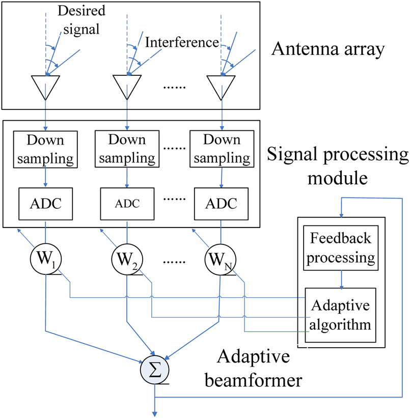
The schematic structure of a linear adaptive antenna array processor on the front end of the receiver is shown in Fig. 1.
The schematic of a linear antenna array processor.

The extracted weight vector is chosen to maximize the output SINR for improving the performance of the ABF, as is given by
 $${\rm SINR} = \displaystyle{{\sigma _S^2 {\vert {{\bf w}^Ha\lpar {\theta_d} \rpar } \vert }^2} \over {{\bf w}^HR_{i + n}{\bf w}}}\comma \;$$
where  $\sigma _S^2 $ is the desired signal power,
 $R_{i + n}$ is the interference plus-noise covariance matrix.
The adaptive beamformer studied here is an inherently multi-objective problem, since multiple sets of agents  ${\bf w}$ with amplitude and phase to make deep nulls toward the interference place and steer the radiation beam toward the desired user to achieve the maximum SINR must be satisfied. On the other hand, all the optimization methods to the designed ABF aim to find the near-global minimum of a mathematical function fit called fitness function; therefore, the best weight vector is determined according to the fitness value obtained from the object function defined based on SINR. In the following sections, the proposed FBS optimization is applied to adjust the weights, such that the fitness function requirements are achieved for obtaining the optimum SINR.
Proposed FBS algorithm
The standard principle of Fibonacci sequence method
The famous Fibonacci sequence was proposed by Leonardoda [Reference Etminaniesfahani, Ghanbarzadeh and Marashi19], the recurrence formula sequence term is given by [Reference Subasi, Yildirim and Yildiz20]
 $$\left\{\matrix{F_1{\rm}= F_2{\rm}= 1 \hfill \cr F_j = F_{\,j-1} + F_{\,j-2}{\rm \comma \;}\quad j \ge 3\comma \;\hfill} \right.$$
where  $F_j$ represents the
 $j{\rm th}$ general term of the Fibonacci sequence.
Fibonacci sequence optimization method makes the tentative optimization points in the defined interval converge to the optimal solution by compressing the search interval proportionally based on Fibonacci sequence term, it has been perceived as one of the most effective strategies to solve the one-dimensional unimodal problem [Reference Yildiz and Karaduman21]. Let us investigate below that how the optimization method using Fibonacci sequence works for a unimodal continuous function in an interval for a minimization problem. Suppose a unimodal  $f\lpar x \rpar $ function is defined on the intervals
 $\lsqb {A\comma \;B} \rsqb $. Initially, the technique starts a choice of two feasible points
 $x_1$ and
 $\widetilde{x}_1$,
 $x_1 \lt \widetilde{x}_1$ in the given range for the first iteration. Then, it is necessary to reduce the initial box of range to a sufficiently small box region including the minimum solution of
 $f\lpar x \rpar $ (through an iteration process) for the interval in which the minimum lies can be narrowed down provided the function values are known at two different points in the range [Reference Omolehin, Ibiejugba, Onachi and Evans22].
Let  $x_p$ and
 $\widetilde{x}_p$ denote the new points over the range of
 $\lsqb {A_p{\rm \comma \;}B_p} \rsqb $ to be chosen for shortening the length of the interval at
 $p{\rm th}$ iteration involving optimal point. Hence for each
 $p = 1{\rm \comma \;}2{\rm \comma \;} \ldots {\rm \comma \;}N$, N represents the maximum number of iterations, Fibonacci algorithm can be executed as:
Step 1 Initialization
Choose
 $\lsqb {{\bf A}_1\comma \;{\bf B}_1} \rsqb {\rm}= \lsqb {{\bf A}\comma \;{\bf B}} \rsqb $ and take $p{\rm}= 1$, while $p \lt N$ do
Step 2 Calculate the iterative points according to the shortening fraction
$F_p/F_{p + 1}$ formed by Fibonacci sequence
(6)$$\eqalign{&x_p = A_p + \left({1-\displaystyle{{F_p} \over {F_{\,p + 1}}}} \right)\lpar {B_p-A_p} \rpar {\rm \comma \;}\cr& \;\widetilde{x}_p = A_p + \displaystyle{{F_p} \over {F_{\,p + 1}}}\lpar {B_p-A_p} \rpar $$Step 3 Find the values
$f\lpar {x_p} \rpar $ and $f\lpar {{\widetilde{x}}_p} \rpar $ using the new pointsStep 4 If
$f\lpar {x_p} \rpar \lt f\lpar {{\widetilde{x}}_p} \rpar $ then $A_{p + 1} = A_p{\rm \comma \;}B_{p + 1} = \widetilde{x}_p$ otherwise $A_{p + 1} = x_p{\rm \comma \;}B_{p + 1} = B_p$.Step 5 Set
$p = p + 1$ then go to step 1 determine whether to stop the iteration






The minimum point of  $f\lpar x \rpar $ can be reached through the steps above for the convergence trend of the tentative points and the linear convergence quality of the Fibonacci optimization strategy.
The basic structure of the proposed Fibonacci branch
The standard Fibonacci strategy cannot solve the multiple variables problem efficiently and retain the optimum fitness evaluation of multimodal function reliably. This is in contradiction to the classic heuristic optimization algorithm. The FBS algorithm, proposed in this paper, is used to overcome these defects while avoiding losing optimal search trajectories by using the searching elements with dendritic branch structure and interactive searching optimization rules.
The basic structure of FBS expanded to the multi-dimensional space D can be illustrated where  ${\bf X}_A$,
 ${\bf X}_B$, and
 ${\bf X}_C$ are the vectors in D dimensional Euclidean space.
 ${\bf X}_A$ and
 ${\bf X}_B$ represent the endpoints of the search element satisfying the optimization rule,
 ${\bf X}_C$ denotes the segmentation points which can be determined from the searching rule. A certain proportion of the vectors can be constructed as follows
 $$\displaystyle{{\Vert {{\bf X}_C-{\bf X}_A} \Vert } \over {\Vert {{\bf X}_B-{\bf X}_A} \Vert }} = \displaystyle{{\Vert {{\bf X}_B-{\bf X}_C} \Vert } \over {\Vert {{\bf X}_C-{\bf X}_A} \Vert }} = \displaystyle{{F_p} \over {F_{\,p + 1}}}\comma \;$$
where  $F_p$ is the
 $p{\rm th}$ Fibonacci number.
Consider the multimodal function with multiple variables  ${\bf f}\lpar {\bf X} \rpar $ to be minimized in search space, the fitness function value calculated by the endpoints in the structure should be evaluated as
 $${\bf f}\lpar {{\bf X}_A} \rpar \lt {\bf f}\lpar {{\bf X}_B} \rpar .$$
Then, the coordinate computing formula of segmentation point  ${\bf X}_C$ can be written as
 $${\bf X}_C{\rm}= {\bf X}_A{\rm}+ \displaystyle{{F_p} \over {F_{\,p + 1}}}\lpar {{\bf X}_B-{\bf X}_A} \rpar .$$
Fibonacci branch search optimization algorithm
The FBS optimization algorithm introduced in this section is based on a framework that is built around the concept of endpoints and segmentation points in the basic structure in Figure 2. Combining with the basic structure, the process of searching for a global optimum solution which can also be regarded as establishing a search element in FBS is to be divided into two stages: local optimization process and global searching process, which are the corresponding two interactive rules. Let G denote the point sets of object function to be searching for in the current processing phase, and set  $\vert G \vert _{num}{\rm}= F_p{\rm \comma \;}\quad i = 1{\rm \comma \;}2{\rm \comma \;} \ldots {\rm \comma \;}N{\rm \comma \;}\;\vert \cdot \vert _{num}$ represents the total number of the set, N is the depth of the Fibonacci branch. The fitness values of the endpoint
 ${\bf X}_A$ and
 ${\bf X}_B$ are initialized using the interactive optimization rules, then the segmentation points
 ${\bf X}_C$ can be obtained from equation (9). By comparing the fitness values of each point in the structure, we can get the results such that the best fitness value accordingly corresponds to the closest optimal solution. To the next optimization phase, the optimal point with best fitness value is provided in the forefront position of the set, and the points corresponding to the suboptimal fitness are arranged below the optimal point in order from best to worst. Throughout the operations above, the points set G can be updated in every optimizing phase growing the Fibonacci branch and global optimization in search space simultaneously.
Basic structure of the proposed FBS.

The two interactive searching rules of FBS in the optimization stage are summarized as follows:
Rule one: Let us consider the endpoints
${\bf X}_A$ and ${\bf X}_B$ in the structure, and defined by


 $$\lcub {{\bf X}_A} \rcub {\rm}= {\rm G}_p = \lcub {{\bf X}_q\vert q = \lsqb {1{\rm \comma \;}F_P} \rsqb } \rcub $$
 $$\lcub {{\bf X}_B} \rcub {\rm}= \left\{{{\bf X}\vert {\bf X}\in \prod\limits_{\,f = 1}^D {\lsqb {X_{lb}^f \comma \;X_{ub}^f } \rsqb } } \right\}\comma \;$$
where  ${\rm G}_p$ is the search points space set in the
 $p{\rm th}$ iteration,
 ${\bf X}_q$ are the points in the set
 ${\rm G}_p$, q is the sequence number that lies in the interval between 1 and the
 $p{\rm th}$ Fibonacci number.
 ${\bf X}_A$ take all the points from
 ${\rm G}_p$ of the
 $p{\rm th}$ iteration. The other endpoints
 ${\bf X}_B$ take random points in search space and the number of
 ${\bf X}_B$ is equal to
 $F_P$. D is the dimension of the points,
 $X_{ub}^f $ are the upper bound and lower bound of the search points. Given that
 $\forall {\bf X}\in \lcub {{\bf X}_B} \rcub $, the component x of the vector
 ${\bf X}$ is a random variable that satisfies a uniform distribution over the interval
 $\lsqb {X_{lb}\comma \;X{}_{ub}} \rsqb $, and the probability distribution of the component can be written as
 $$P\lpar x \rpar = U\lpar {X_{lb}{\rm \comma \;}X{}_{ub}} \rpar = \displaystyle{1 \over {X{}_{ub}-X_{lb}}}.$$
Using the given endpoints  ${\bf X}_A$ and
 ${\bf X}_B$, we can determine the segmentation points
 ${\bf X}_{S1}$ in the first global search stage by equation (11).
Rule two: Suppose  ${\bf X}_{{\rm best}}$ is the optimal solution corresponding to the best fitness value of the search space in the current iteration containing the endpoints and the segmentation points generated from rule one, as given by
 $${\bf X}_{{\rm best}}{\rm}={\rm BEST}\lpar {{\bf G}_P} \rpar \comma \;$$
where  ${\rm BEST}\lpar{\cdot} \rpar $ means the best solution of the set at
 $p{\rm th}$ iteration.
Then, we set the endpoints  ${\bf X}_A{\rm}= {\bf X}_{{\rm best}}$ and have that:
 $$f\lpar {{\bf X}_A} \rpar = {\rm min}\lcub {\,f\lpar {{\bf X}_q} \rpar {\rm \comma \;}q = \lsqb {1\comma \;F_P} \rsqb } \rcub $$
 $${\bf X}_B = \lcub {{\bf X}_q\vert {\bf X}_q\in {\bf G}_P\wedge {\bf X}_q\ne {\bf X}_A} \rcub .$$
Hence, the segmentation points  ${\bf X}_{S2}$ in the second local optimization stage can be determined based on the endpoints defined by (14) and (15) using the computing formula of segmentation points.
From the two interactive searching rules mentioned above, new points including endpoints  ${\bf X}_A$,
 ${\bf X}_B$ and segmentation points
 ${\bf X}_{S1}$,
 ${\bf X}_{S2}$ are generated in the two optimization stages, and the total number of the points is
 $3F_P$. Evaluating the cost functions in new points determines their fitness, all these points are sorted from the best to the worst based on their fitness value. The population size of the search points is chosen as the Fibonacci serials; thus, the top best
 $F_{P{\rm +}1}$ sets of these points are to be saved and the rest corresponding
 $3F_P-F_{P{\rm +}1}$ points need to be dropped. After this procedure, the sets of the search space in the current
 $p{\rm th}$ iteration are renewed from the saved points, e.g. the saved points form a new set
 ${\bf G}_{P{\rm +}1}$ in search space for the next iteration.
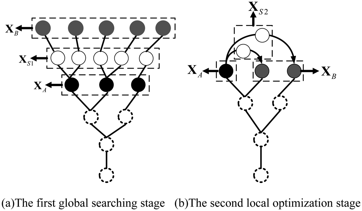
The two stages of building the Fibonacci branch for the global optimization in space are shown in Fig. 3.
The process of building the Fibonacci branch for global optimization. (a) The first global searching stage. (b) The second local optimization stage.

As can be seen from Fig. 3, the depth of the Fibonacci branch layer illustrated in the figure is initialized as expected, and the number of the points in every branch layer is kept to the sequence of Fibonacci number. The white dashed circle in the figure represents the search points set of the previous iteration, the black solid circle denotes the endpoints  ${\bf X}_A$ in the current iteration, and the global random endpoints
 ${\bf X}_B$ are represent in the gray solid circle. Figure 3(a) shows the first global searching stage of the global optimization process, the segmentation points
 ${\bf X}_{S1}$ which are represented by the solid white line circle are constructed on the basis of global random points and
 ${\bf X}_A$. The second local optimization stage is illustrated in Fig. 3(b), with the best fitness points
 ${\bf X}_A$ in the search space of the current iteration and the rest endpoints of
 ${\bf X}_B$, the new segmentation points
 ${\bf X}_{S2}$ can be obtained by iterative rules. The fitness values of
 ${\bf X}_A{\rm \comma \;}{\bf X}_B{\rm \comma \;}{\bf X}_{S1}$, and
 ${\bf X}_{S2}$ are to be evaluated, and the best found
 $F_{P{\rm + }1}$ solutions with optimum object function evaluations need to be saved.
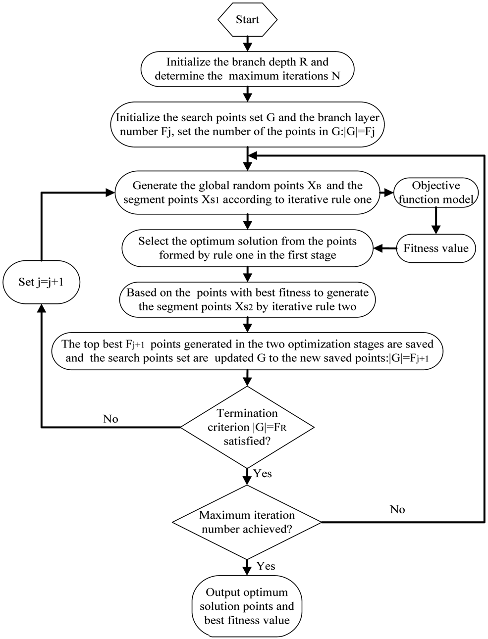
Figure 4 exposes the flowchart of the general procedures for the specific implementation of FBS, and the Pseudo-code of the FBS is shown in Algorithm 1.
Algorithm 1 Pseudo-code of the FBS algorithm
Initialization
1. Determine the maximum iteration number (N) and the depth of the Fibonacci branch (R)
Iteration
2. While predefined maximum number of iterations is not achieved
3. While the termination criterion
$\vert G \vert = F_R$ not satisfied do searching and optimization phase4. Choose the search points set G in the defined space and set the initial number of branch layer
$F_j$5. Calculate the shortening fraction
$F_j/F_{j{\rm +}1}$ and generate ${\bf X}_B$, ${\bf X}_{S1}$ according to rule one6. Measure the fitness of these points based on the objective function model and perform the analysis to identify the optimal points with the best fitness value
7. Take the best points and
${\bf X}_B$ in current points set to generate ${\bf X}_{S2}$ from equation (7) of rule two8. Save the top
$F_{j{\rm + }1}$ points and update the set G to the new saved points for the next branch layer iteration9. Set
$j = j + 1$ and go to the line 310. End while
11. Save the optimum solution points of the current iteration in search set space and go to line 2.
12. End iteration and output the optimal points


The proposed FBS algorithm mentioned above utilizes the interactive global searching and local optimization to obtain the global optimal solution so that it can take advantage of the global randomness and local convergence to get rid of the local minima. The generated points in each layer of the whole branch depend on the optimum elements with the best fitness value in the previous branch layer which can assure the global optimum solution in search space.
Flowchart of Fibonacci branch search optimization method.

FBS-based beamformer design and implementation of ABF with the proposed FBS
As explicitly described previously, ABF is an effective technique used to mitigate interference and improve overall SINR performance by altering the radiation pattern of an antenna array; however, typically, the low nulling levels toward multiple interference sources and non-globally optimal weight vector are two major drawbacks of the MVDR beamforming technique [Reference Jayaprakasam, Abdul Rahim, Leow and Ting23]. Therefore, the proposed FBS algorithm is applied to the ABF with ULA in this section for achieving the improved performance of this technique.
ABF model integrated with FBS
The description of the beamforming model has already been given in section “ABF system model of ULA and problem statement”, each adaptive beamformer in the model aims at calculating the complex weight vector that satisfies the requirement of maximizing the output SINR; in this work, the proposed FBS incorporated into the beamforming model will extract the best array excitation weights through maximizing the objective function based on SINR.
Equation (16) indicates how the ABF design problem is setup for the FBS-based optimization.
 $$X_{mF_i} = w_m{\rm \comma \;}\quad m = 1{\rm \comma \;}2 \ldots {\rm \comma \;}M{\rm \comma \;}F_i \le {\kern 1pt} F_R\comma \;$$
where  $w_m$ is the
 $m{\rm th}$ excitation weight of the array element.
 $X_{mF_i}$ is the
 $F_i{\rm th}$ search point at the
 $m{\rm th}$ dimension of the
 $i{\rm th}$ branch layer,
 $M{\kern 1pt} $ is the total number of ULA, R is the depth of the branch. The weights are interpreted here as the optimization points of the Fibonacci branch in the search space. The initial population of the weights is determined by the layer I with
 $F_I$ search points, and the weight vectors of entire population generated as the search points at the first layer can be written in the format as below:
 $${\bf W}_{MF_I} = \left[{\matrix{ {w_{11}} & {w_{12}} & \ldots & {w_{1F_I}} \cr {w_{21}} & {w_{22}} & \ldots & {w_{2F_I}} \cr \vdots & \vdots & {} & \vdots \cr {w_{M1}} & {w_{M2}} & \ldots & {w_{MF_I}} \cr } } \right]\comma \;$$
where  ${\bf W}_{MF_I}$ is the weight vectors containing
 $F_I$ agents with M sensors representing the dimension of the search points, e.g. every agent will have the M weight elements.
 $F_I$ is the
 $I{\rm th}$ Fibonacci series chosen as the total number of the points at the first layer of the Fibonacci branch. Each complex weight of
 ${\bf W}_{MF_I}$ in the array element has amplitude and phase. Then, the proposed new optimization algorithm FBS is deployed to adjust the current amplitude and phase coefficients of the weight factor to provide the maximum beam pattern toward desired signals as well as making the deep nulls toward the undesired ones to achieve the maximum SINR. Thus, the optimization formulation process of the ABF problem will try to maximize the fitness function constructed from the perspective of the SINR accordingly for the calculation of the complex excitation weight using FBS, and the fitness function designed in this text can properly be stated in the following form
 $${\rm Fitness}\_{\rm Function}\lpar {\bf w} \rpar = \displaystyle{{P_d} \over {\sum\nolimits_{i = 1}^Q {P_i + P_N} }}\comma \;$$
where
 $$P_d{\rm}= \displaystyle{1 \over 2}E\lsqb {{\vert {{\bf w}^T{\bf X}_d} \vert }^2} \rsqb $$
 $$P_i{\rm}= \displaystyle{1 \over 2}E\lsqb {{\vert {{\bf w}^T{\bf X}_i} \vert }^2} \rsqb $$
are, respectively, the power of the desired signal and the power corresponding to the  $i{\rm th}$ interference,
 $P_N$ is the noise power.
 ${\bf X}_d$ and
 ${\bf X}_i$ denote the desired signal and interference component of the received signal in equation (1)
Then, the design objective function (18) can properly be stated in the following form
 $${\rm Fitness}\_{\rm Function}\lpar {\bf w} \rpar {\rm}= \displaystyle{{{\bf w}^T{\bf R}_d{\bf w}} \over {{\bf w}^T\sum\nolimits_{i = 1}^Q {{\bf R}_i{\bf w} + \sigma _{noise}^2 {\bf w}^T{\bf w}} }}\comma \;$$
where  ${\bf R}_i$ and
 ${\bf R}_d$ are the covariance matrix of the
 $i{\rm th}$ interference and the desired one. The noise variance is calculated from the value of signal-to-noise ratio (SNR) in dB as follows:
 $$\sigma _{noise}^2 = 10^{{-}SNR/10}.$$
In addition, an important feature of the beamformer is that it can form the desired radiation beams, such as the formation of the low sidelobe beams and the flat-top beams. Thus, the next step in the design process is to formulate the other objective function that is to be minimized for the sidelobe reduction problem. An array consisting of identical and identically oriented elements has a far-field radiation pattern that can be expressed as the product of the element pattern and a factor that is widely referred to as the array factor. The objective function we defined used the array factor in such a way that the objective of the optimization is satisfied. The fitness function to be minimized with the optimization algorithms to introduce the deeper null and reduce the relative sidelobe level (SLL) is given in
 $${\rm Fitnes}{\rm s}_{SLL} = \sum\limits_k {\vert {AF\lpar {\theta_k} \rpar } \vert + 10{\rm lo}{\rm g}_{ 10}\left({\displaystyle{{AF\lpar {\theta_{MSL}} \rpar } \over {AF\lpar {\theta_{ML}} \rpar }}} \right)} \comma \;$$
where  $\theta _k$ is the direction of the interference,
 $\theta _{MSL}$ is the angle of the maximum SLL,
 $\theta _{ML}$ is the angle of mainlobe.
 $AF\lpar \theta \rpar $ is the array factor of the uniform linear array, and can be written as [Reference Jayaprakasam, Abdul Rahim, Leow and Ting23]
 $$AF\lpar \theta \rpar {\rm}= \displaystyle{1 \over Q}\sum\limits_{q = 1}^Q {w_q{\rm e}^{{-}j{{2\pi } \over \lambda }\lpar {q-1} \rpar d{\rm cos}\lpar {\theta -\varphi_q} \rpar }} \comma \;$$
where Q is the number of array elements,  $\theta $ is the angular region of interests.
 $w_q$ is the weight at the element q.
 $\varphi _q$ determines the excitation phase of the
 $q{\rm th}$ element.
Consequently, for array design with suppressed SLL and deep null control simultaneously, both terms of equation (23) are used in the fitness evaluation. By optimizing the fitness function defined in this section, the optimal excitation weight corresponding to the minimum level of the interference sources and lowest SLL but with the desired user gain of the beamformer can be achieved by the proposed FBS optimization algorithm. Next section of the paper provides a brief description of the implementation steps for extracting the weight using FBS method.
Implementation flowchart of Fibonacci branch search to ABF
In this subsection, in light of the results described in detail previously, an optimization scheme of ABF problem that combines with the novel FBS is presented to enhance the maximum power for target signal and generate deep nulls for interferences with the lowest sidelobe. The basic idea of the design of such an adaptive beamformer is to utilize the global searching and local convergence capability of the novel efficient search algorithm to reduce the local minimum problem of the solution to weight vector and satisfy the requirements to the created multi-objective optimization problem from (21) and (23) for getting the maximum SINR and the minimum SLL. The general procedures for the implementation of the FBS method with application to ABF are presented in Fig. 5, in which the key steps are briefly described below.
(a) Choose the depth R of Fibonacci branch to determine the population
$F_R$ of the top branch layer, and set the maximum number of iterations of the optimization process.(b) Initialize the population of the first branch layer
$F_j$ and determine the dimension of the weight vectors acted as search points in space according to the element number of ULA. Also, define the amplitude search space of the weight within $\lsqb {0{\rm \comma \;}1} \rsqb $ and limit the range of weight phase to $\lsqb { - \pi {\rm \comma \;}\pi } \rsqb $.(c) Assign the values to the amplitude and phase of the weight elements inside the search space for constructing the initial population of the weight vector set
${\bf G}_{\bf w}$, the weight element in the vector sets ${\bf G}_{\bf w}$ constructed by the amplitude and phase can be expressed as follows:
(25)$${\bf w}_{\,j{\kern 1pt} d} = {\rm r \;and}\;\lsqb {0{\rm \comma \;}1} \rsqb \cdot {\rm e}^{\,j\cdot {\rm rand\lsqb } \hbox{-} \pi {\rm \comma }\pi \rsqb }\comma \;$$


where the generated weight  ${\bf w}_{j{\kern 1pt} d}$ represents the dth dimension of the jth individual in the population, d ∈ [1, M(dimension of the search space)], j ∈ [1, F j(population of the vectors)], rand [·] denotes the random value generation in the range.
(d) Take the random amplitude and phase values in search space for generating the
$F_j$ population of the weight vectors ${\bf w}_B$ which is acted as the global search points.(e) Set the vector elements of
${\bf G}_{\bf w}$ and ${\bf w}_B$ as the endpoints in equation (9) and compute the first set of weights ${\bf w}_{S1}$ according to the iterative rule one.(f) Calculate the fitness in the object function of (21) and (23) using
${\bf G}_{\bf w}$, ${\bf w}_B$, and ${\bf w}_{S1}$, then give the evaluation to the values to find the best weight vector ${\bf w}_{best}$ with the maximum fitness value among all the vectors in space.(g) Generate the second set of weight vectors based on the best weight vector
${\bf w}_{best}$ and the other weights from the weight space set using equation (9) in iterative rule two.(h) Select the top
$F_{j{\rm +\ }1}$ best weight vectors depending on the maximum fitness value in the optimization process and these best weights are selected to compose the new population of the set ${\bf G}_{\bf w}$.(i) Check the termination criteria
${\bf G}_{\bf w}{\rm}= F_R$. If the termination criteria not satisfied, then increment j and go to step (d). Otherwise, stop.(j) If the maximum number of iterations is not reached, repeat the algorithm from step (d), or else report the output results and terminate.


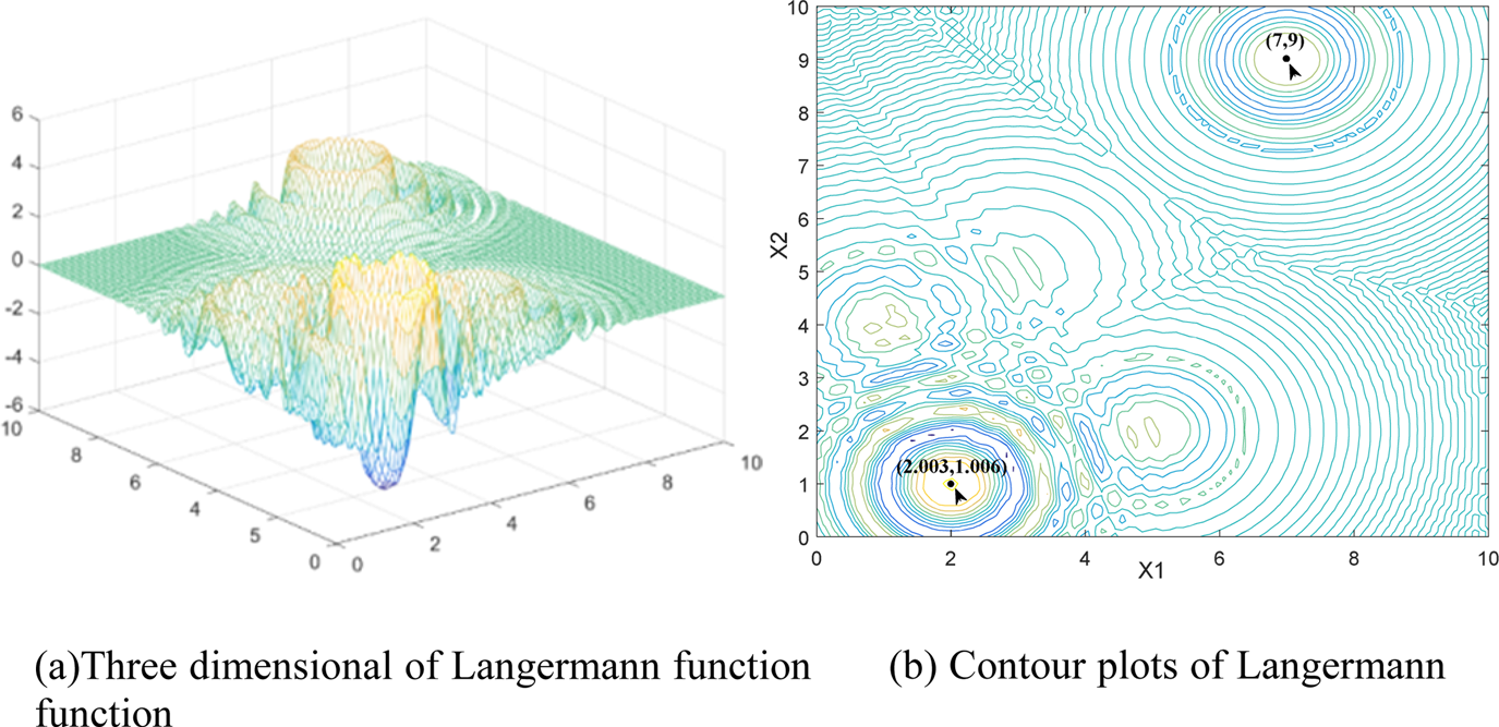
Three-dimensional and contour plots for the Langermann function. (a) Three-dimensional plots of Langermann function. (b) Contour plots of Langermann function.

Simulation results
Verification of the proposed FBS
In order to validate and analyze the efficiency and effectiveness of the proposed FBS, the algorithm is verified from the following aspects in simulation experiments:
(1) The accessibility to the global optimum of the proposed search algorithm for multimodal function with numerous local optima is revealed by the location history of the search points toward the optimal point.
(2) The convergence of the FBS is proved and discussed by the presented gradient of the iteration curves which manifested the convergence rate speed and the average fitness of the chosen benchmark function.
(3) The optimization precision of the solution and other relevant optimization assessment aspects of the proposed algorithm are tested on eight representative standard benchmark functions and the results are compared with the typical heuristic algorithms.
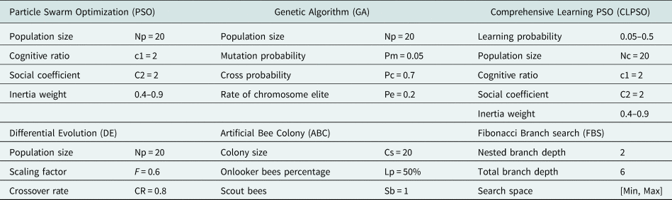
The details of the parameter settings for every heuristic algorithm used in the experiments are given in Table 1.
Reference parameters of the algorithms briefly used in this study

All the experimental tests are implemented on Intel (R) Core (TM) i7-7700 HQ Core Processor at 2.8 GHz and 2.8 GB RAM, and all the MH algorithms are coded and carried out in Matlab 2017b version under the Windows10 Professional.
The location history of the search points in FBS for Langermann function
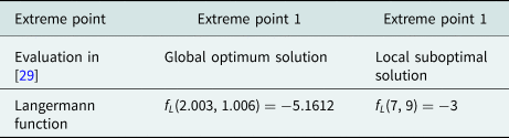
In this section, the global optimization ability of the proposed FBS is demonstrated by employing the location history of the search points during optimization process for locating the global optimum solution rather than trapping into local optimization of the benchmark example, with results compared against metaheuristic PSO algorithm. The benchmark function chosen in this section is the Langermann function with several known local optimal points and one global optimum solution point which is taken from [Reference Adorio and Diliman24, Reference Molga and Smutnicki25] and is summarized in Table 2. As can be found in Table 2, two typical extreme points existed in the function, the extreme point 1 shown in the table is the global optimum solution, and the extreme point 2 is the local suboptimal solution. The three-dimensional Langermann function and contour plots are illustrated in Fig. 5.
Langermann benchmark function

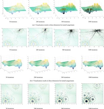
The performance of the proposed FBS in terms of the movement trajectory of the search points scattering around the best solutions and converge toward the optimal point in the search space for Langermann is illustrated in Fig. 6(b). This figure shows that the FBS model is able to simulate the position history of search points in three-dimensional and trajectory contour plots over different iterations. For the verification of the results, we compare our algorithm to PSO with these same works and provide the results in Fig. 6(a). The initial position of the search points in both FBS and PSO is set at the extreme point 2.
Location history of the search points in three-dimensional and contour plots for the Langermann function over the course of different iterations. (a)Three-dimensional plots of Langermann function. (b) Contour plots of Langermann function. (a).1 Visualization results in three dimension for tested Langermann. (a).2 Visualization results in contour plots for tested Langermann. (a) Behavior results of the points location history in PSO. (b).1 Visualization results in three dimension for tested Langermann. (b).2 Visualization results in contour plots for tested Langermann. (b) Behavior results of the points location history in FBS.

As the results exhibited in Fig. 6, the search points tend to explore the promising regions of the search space and cluster around the global optima eventually in multimodal Langermann pattern. From the results depicted in Fig. 6(a), we can know that as the number of iterations increases, the points of PSO algorithm gradually cluster around the extreme point 2 and proceed toward local optima, and almost no particles enter the region near the global optimum extreme point 1, reflecting the further evidence that PSO inherently suffer from local optima entrapment and stagnation in the search space. Under the same conditions, it can be seen from the trajectories and 3D version of the search points as shown in Fig. 6(b), although the Langermann function is non-symmetry and multimodal with different levels of peaks; finding its global optimum is challenging due to many local minima in the search space; remarkably, FBS is to be extricated from initial local optimum at extreme point 2 and jump out of the trapped solution in a local optimum point assisted by global random searching; it is evident from the location history of the search points during the process of converging toward the global optima that the points grow toward the optimal point from the area of initialization, tending to scatter around extreme points gradually and moving toward the best solutions in the search space in both 2D and 3D spaces over the course of iteration. More than half of the agents had already approached the global optimum valley after the first 50 iterations and begun converging on the optimum. As iteration increases, there are more agents that aggregate at the extreme points and scatter around the extreme point, especially attracted intensively at the global optimum target region. Eventually, the search points found the global optimum and converged toward the global optima. This can be discussed and reasoned according to the global randomness concepts introduced by the endpoints  ${\bf X}_B$, which is generated in rule one of FBS; furthermore, the convergence of FBS is guaranteed by the local exploitation optimization ability emphasized in the other endpoints
 ${\bf X}_A$ of the proposed algorithm. Since the global random points tend to move from a less fit universe to a more fit universe by global searching in space, the best universe is saved and moved to the next iteration. Consequently, these behaviors and abilities will assist the FBS not to become trapped in local optima and converge toward the target point quickly in the iterations of optimization.
The above simulations and discussions demonstrate the effectiveness of the FBS algorithm in finding the global optimum in the search space; the convergence performance and the rate of obtaining the global optima of the proposed algorithm by employing a set of mathematical functions are to be investigated in the next sections.
Convergence performance of the multimodal function
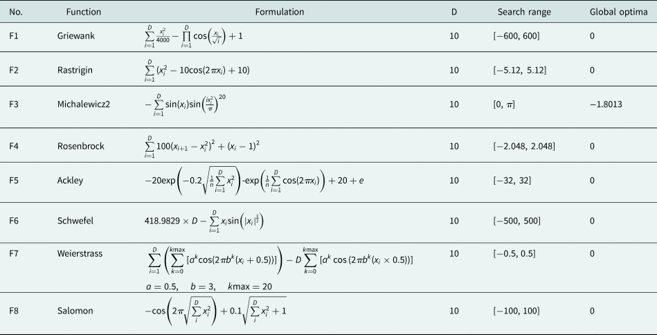
To confirm the convergence behavior of the proposed algorithm, in this subsection, we provide the convergence curve objective fitness value of the typical benchmark functions obtained by the best solutions so far in each iteration. A large set of complex mathematical benchmark functions to be tested is listed in Table 3. These functions have many local optima which make them highly suitable for benchmarking the performance of the metaheuristic algorithms in terms of optimization and convergence exploration. The illustrated results are compared against that of PSO, GA, CLPSO, DE, and ABC metaheuristic algorithms on the same set of multi-dimensional numerical benchmark functions. The properties and the formulas of these functions are presented below.
The details of multimodal benchmark functions (D: dimensions)

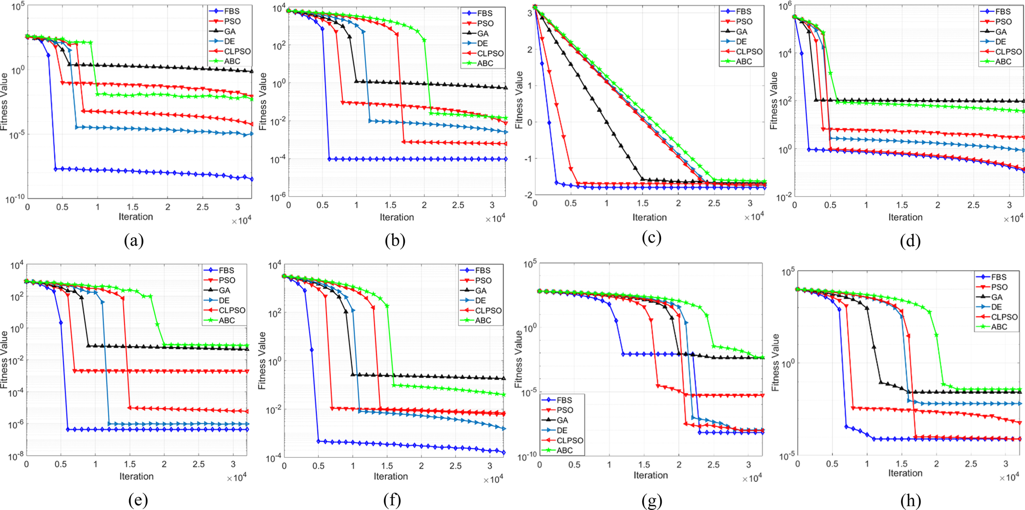
Figure 7 presents the convergence characteristics in terms of the best fitness value of the median run of each algorithm for the test functions. Comparing the results and the convergence graphs, among these six algorithms, we observe that the proposed algorithm has good global search ability and converges fast. FBS achieved better results on all multimodal groups than the comparison algorithms, it surpasses all other algorithms apparently on functions 1, 2, 5, and 6, and especially significantly improves the results on functions 1 and 2. The other algorithms show poor performance on the complex problems since they miss the global optimum basin to approach the optimal fitness. The Schwefel's function is a good example, as it traps all other algorithms in local optima, while the FBS successfully avoids falling into the deep local optimum which is far from the global optimum. On the complex multimodal functions with randomly distributed local and global optima, FBS performs the best. It should also be noted that the FBS algorithm in the graphs exhibited the superiority regarding the convergence speed over the other five algorithms, it converges to a global optimum solution with less fitness evaluations and terminates after no more than 5000 iterations on functions 1, 3, and 4, and always converges faster than others on the remaining functions.
Convergence behavior of the FBS and other optimization algorithms on 10-D benchmarking functions F1–F8. (a) F1: Griewank; (b) F2: Rastrigin; (c) F3: Michalewicz2; (d) F4: Rosenbrock; (e) F5: Ackley; (f) F6: Schwefel; (g) F7: Weierstrass; (h) F8: Salomon.

These figures also prove that FBS not only improves the accuracy of the approximated optimum initial, but also desirably enhances the convergence speed over the course of iterations that make it converge faster than the other algorithms. Global random property and space region shortening fraction guarantees a satisfactory convergence speed. Other algorithms could not converge as fast as the FBS, since they have a large potential search space. The proposed FBS combines global searching method and local optimization strategy together to yield a balanced performance that achieves better fitness and faster convergence. Besides, the convergence speed is a crucial parameter of real-time applications like ABF system; thus, the FBS is highly suitable and affordable for ABF.
Minimization result of the tested benchmark functions
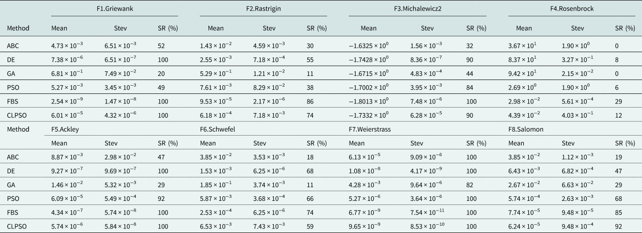
In this subsection, experiments were conducted on a suite of multimodal functions illustrated in Table 3 to evaluate six optimization algorithms including the proposed FBS. All the test functions are to be minimized and the relevant information can be found in [Reference Cui, Li, Wang, Lin, Chen, Lu and Lu26, Reference Zhang, Ning, Lu, Ouyang and Ding27] for the standard benchmark functions, respectively. For the selected benchmarking problems F1–F8, the dimension of these functions is set to 10. Every algorithm runs 1000 times independently to reduce the statistical error and achieve reliable results.
The statistical results considering the average value and the standard deviation function fitness value as well as the success rate needed to reach the acceptable solution are summarized in Table 4. For the results shown in Table 4, the mean value is smaller, the performance of the algorithm is better. The standard deviation value is lower, the stability of the algorithm is stronger. As seen, for most benchmark data sets, the average value and the standard deviation calculated by the FBS are both smaller than those for other algorithms, and the proposed algorithm surpasses all other algorithms on functions 1, 2, 3, 5, 6, and 7, and especially significantly improves the results on functions 1 and 3. When the other algorithms find their own best fitness of these functions, the proposed FBS could still search the better fitness closest to the optimal value. The CLPSO achieved the similar results as the FBS on function 7, and they both are much better than the other variants on this problem. The DE also performs well on multimodal problems. The DE performed similarly with the FBS on functions 1, 3, 5, and 7. However, the FBS performs better on much more complex problems when the other algorithms miss the global optimum basin.
The comparative and statistical results for benchmarking function problems F1–F8

As a result, in terms of performance in the global search ability and the optimization stability for benchmarking function, the proposed FBS outperformed all other heuristics algorithms on the tested functions. Also, this table illustrates that FBS in comparison with others displays the highest percentage and accuracy of reaching to the acceptable solutions on these test functions. For the mean reliability of test functions F1, F3, F5, F7, FBS exhibits the highest reliability of 100% success rate and smallest average errors. This performance superiority property is due to the FBS's interactive updating rule. With the new updating rule and global randomness, different dimensions may learn from different exemplars based on the historically optimal search experience, and the FBS explores a larger search space than the other comparisons. Because of this, the FBS performs comparably to or better than many MH algorithms on most of the multimodal problems experimented in this section.
The performance of the FBS in ABF model application
To demonstrate the benefits of the FBS optimization with application to ABF, in this part of the section, several groups of simulation experiments are conducted using Matlab R2017b. The performance of the FBS-based ABF was evaluated from the following two simulation metric aspects: the beampattern performance of the adaptive antenna array and the steady state output SINR of the beamformer system. A uniform linear array with the inter-element spacing of half wavelength is considered in the simulation. The desired signal is in the form of QPSK modulation mode with 0° for incident azimuth angle and the three single frequency interfering sources with 10 interference-to-noise (INR) ratio are assumed to impinge on the antenna array from the azimuth directions  $20{\rm \comma \;}40^\circ $, and
 ${-}20^\circ $, respectively. The desired signal and jammers are all arranged to be coming from zeniths
 $45^\circ $. Simulation environment is the additive white Gaussian noise channel.
The proposed FBS-based beamforming method is compared with the following four conventional heuristics-based beamforming algorithms: (1) the differential evolution (DE)-based beamforming method of [Reference Zhang, Ning, Lu, Ouyang and Ding27], (2) the particle swarm optimization (PSO)-based beamforming method of [Reference Mallipeddi, Lie, Suganthan, Razul and See28], (3) the comprehensive learning particle swarm optimization (CLPSO)-based beamforming method of [Reference Banerjee and Dwivedi29], (4) the artificial bees colony (ABC)-based beamforming method of [Reference Ismaiel, Elsaidy, Albagory, Atallah, Abdel-Rahman and Sallam30], and (5) Genetic Algorithm (GA)-based beamforming method of [Reference Ruchi, Nandi and Basu31]. A total of 300 repetitions are implemented and then averaged to obtain each figure of the results.
Beampattern performance results
In this subsection, the effectiveness and applicability of the proposed FBS-based beamformer are investigated by the power patterns formed by different types of the metaheuristic-based beamformers. The determined optimized antenna element current amplitudes are applied to minimize the peak SLL and to place nulls in the desired directions based on the MATLAB platform, the optimized results are compared with the above-mentioned algorithms. Four groups of simulation cases conducted in terms of various simulation metrics are considered in this study. The first simulation example is with different number of interference sources and the second case considers the different number of array elements. The performance measurement on the input SNR is studied in the third case. The last case illustrates the sidelobe reduction and deep nulls executed by the optimization algorithms based on fitness function (23).
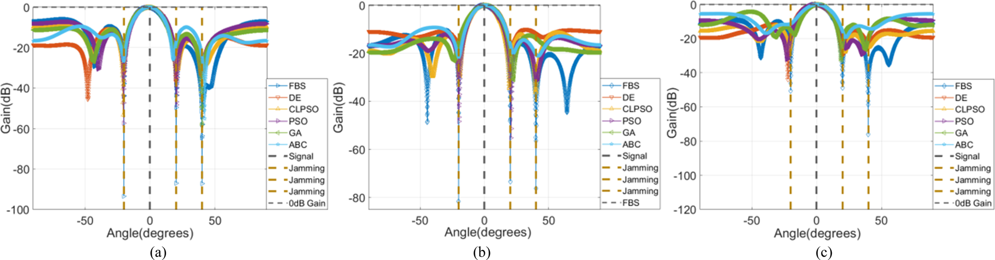
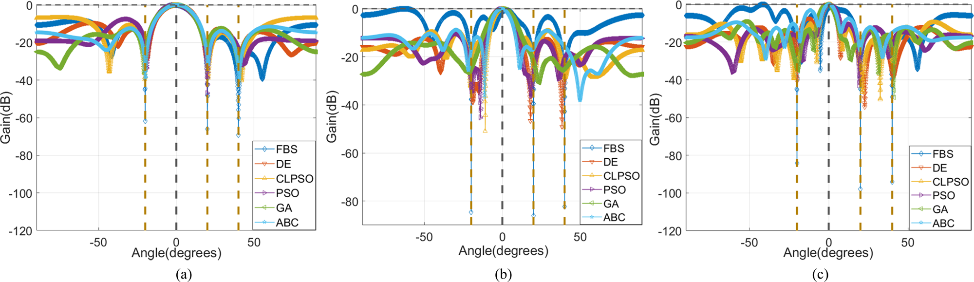
Simulation case one: input SNR evaluation: We first examine the beampattern performance synthesized by the FBS and compared to the others given in [Reference Mallipeddi, Lie, Suganthan, Razul and See28–Reference Lu and Yeo32] in terms of input SNR in this case. A uniform linear array with six omni-directional antenna elements is considered in the simulation. For investigating the effect of the input SNR with different levels, we consider three sets of input SNR with  $SNR ={-}30\,{\rm dB\comma \;}\;SNR ={-}10$, and
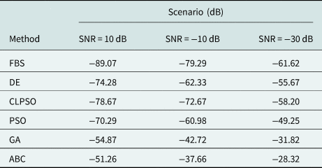
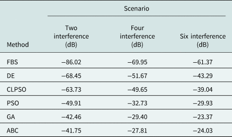
 $SNR = 10$ to check the validity of our approach. Figure 8 shows the behavior of the beampatterns synthesized by the weight vectors determined by the optimization algorithms under different SNR, and to more clearly illustrate the nulling degrees and nulling level of each method, the nulling results corresponding to Fig. 8 are shown in Table 5. It can be seen from the figures that the weight vectors found by FBS could synthesize the inerratic beampattern with deeper nulling (with nulling level exceeding −70 dB) toward the interference compared to the other algorithms. The proposed FBS-based adaptive beamformer has suppressed the jammers in all cases while maintaining the beampattern gain in the direction of the desired signal. The other algorithms are able to achieve the interference nulling performance for a higher SNR level, i.e. SNR = 10, as the level of SNR decreases, the compared beamformers, especially ABC-based beamformer and GA-based beamformer, suffer from performance degradation of the corresponding metaheuristic-based beampatterns, and the nulls do not align precisely with the interference sources. This indicates that the proposed algorithm is more stable and finds better solutions with greater precision in ABF application.
Comparison of the beampattern performance synthesized by the heuristic algorithms with different SNR. (a) SNR = 10 dB; (b) SNR = −10 dB; (c) SNR = −30 dB.

Comparison of average nulling level toward interference sources for different SNR scenarios

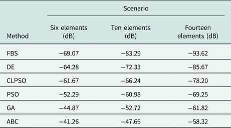
Simulation case two: array element number investigation: Beampattern performance regarding the number of array elements has been evaluated in the second case study; adaptive beamformer arrays that consist, respectively, of 6, 10, and 14 were concerned in the simulation experiments. Input SNR was fixed −5 dB. The proposed FBS in comparison with the other metaheuristic algorithms is applied to search for the optimum element phases and amplitude of the uniform linear array to achieve target pattern by considering these three cases with different element numbers. Optimization results of the beampatterns are illustrated in Fig. 9. To avoid showing the confusing results and better distinguish the nulling level, Table 6 illustrates the specific nulling level in different array elements scenarios. The results depicted in Fig. 9 show that the proposed FBS achieves better performance than the other algorithms with the same number of array elements. It means FBS possesses superior performance as compared to DE, CLPSO, GA, PSO, and ABC because it creates deeper null toward the interference direction while maintaining the power at the desired direction. As the number of the elements increases from 6 to 14, the beampattern formed by the other methods particularly for the ABC and GA are deteriorating and almost fail to work in steady state, that is, the performance disparity between proposed algorithm and the compared algorithms is expected to increase further with higher number of array elements, this is due to the increase of the number of elements results in the increase of searching dimension of the solution, which inherently increases the difficulty of the optimization problem, and the global search optimization ability of the FBS algorithm is more suitable for the multi-dimensional solution of the large array elements to improve the beampattern performance.
Comparison of the beampattern performance synthesized by the heuristic algorithms with a different number of array elements. (a) Six elements; (b) 10 elements; (c) 14 elements.

Comparison of average nulling level toward interference sources for different array elements scenarios

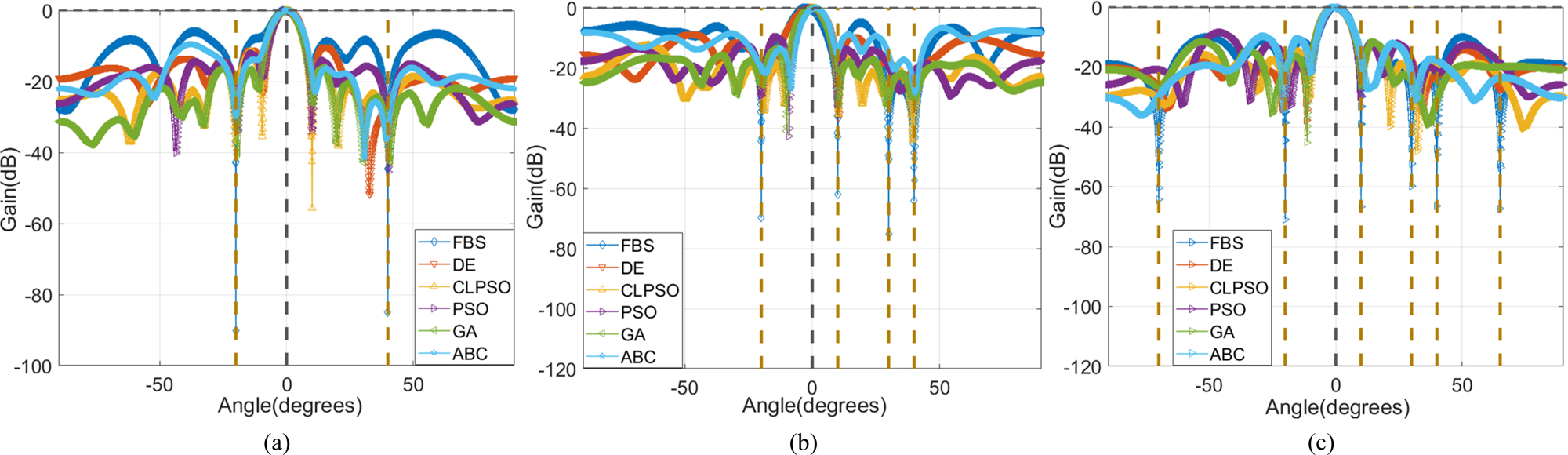
Simulation case three: interference sources number assessment: In order to fully verify the beampattern performance, different types of multiple interference scenarios were simulated to validate the proposed approach for ABF applications in this case. A uniform linear array of 12 omni-directional antenna elements was adopted in this subsection. All scenarios have one desired signal at  $\theta _s = 0^\circ $ while the number of interference changes in each one. The first two target interferences source is assumed to be impinging on the array from
 $ - 20$ and
 $ 4 0^\circ $, and the four received interferences that impinge at
 $\theta _i = \lcub {2 0^\circ \comma \;4 0^\circ \comma \;- 2 0^\circ \comma \;30^\circ } \rcub $ are considered in the second scenario, finally, the third scenario concerns six interferences with incident angle
 $\theta _i = \lcub {2 0^\circ \comma &mathbreak;\;4 0^\circ \comma \;- 2 0^\circ \comma \;30^\circ \comma \;6 5^\circ \comma \;- 7 0^\circ } \rcub $. In each scenario, the FBS and other optimization algorithms are applied to find the optimal excitation vectors, respectively, that produce a main lobe toward
 $\theta _s$ and nulls toward
 $\theta _i$. The graphs shown in Fig. 10 represent the optimized beampattern for all the scenarios studied here. All the radiation pattern results presented in Fig. 10 show that FBS-based beamformer is a robust technique capable of improving the radiation characteristics with better performance than the conventional optimized beamformer whatever the number of interference signals is. The FBS-based beamformer exhibits more prominent behavior regarding the steering ability increasing the nulling levels in Fig. 10(c), i.e. the superiority of FBS in scenario 3 is more apparent than the other two cases. When the number of interference sources increases, it is more difficult for the other optimization algorithms to enhance the null level in the interference direction. Therefore, these results demonstrate that the superior exploratory and exploitive properties of FBS applied to ABF have resulted in better beam-steering and interference mitigation performances in all three cases, especially for the multiple interference sources.
Comparison of the beampattern performance synthesized by the heuristic algorithms with a different number of interferences. (a) Two interferences; (b) four interferences; (c) six interferences.

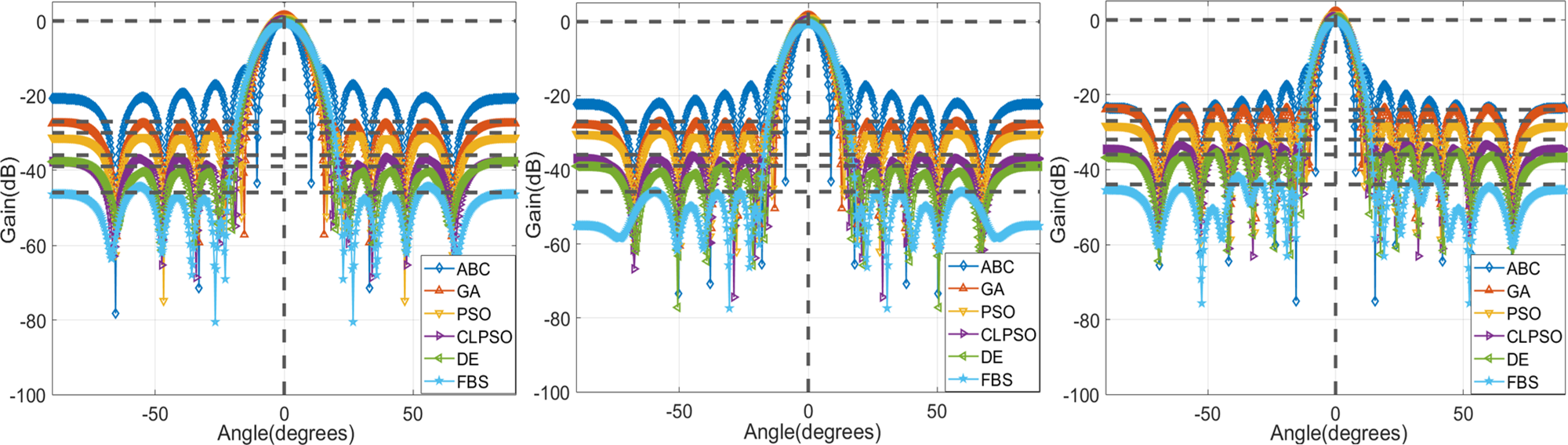
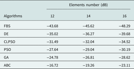
Simulation case four: evaluation of the SLL of the beampattern: The proposed FBS and other selected comparison algorithms in the last case determine the weight of each array element for achieving the lower sidelobe. The receiving linear antenna arrays composed of 12, 14, and 16 monochromatic isotropic radiating elements considered for reference in different simulation scenarios. Suppose four interferences from respective different angles impinge on the ULA, each scenario has one desired signal at  $\theta _s = 0^\circ $. The INR of all the simulation scenarios is fixed at 30 dB. Figure 11 displays the graphical beampattern comparison of the optimized array factor with reduced SLL. It can be seen from Fig. 11 that the symmetry of array factors makes the array radiation pattern more regular than the conventional beamformers, and the proposed FBS provides a better reduction in SLL as compared to arrays optimized using other algorithms; also, it is observed from the figure that null depth in the interference direction synthesized by FBS is superior to the others. The following Table 7 and Table 8 show the specific values of the maximum SLL of each algorithm for the ULA. The simulation results in the table confirm the superiority of the proposed FBS via specific maximum SLL and reduction degrees. The maximum SLL obtained using the FBS with 12, 14, 16 elements is −43.68, −45.62, −48.29 dB, respectively, and the improvement of sidelobe reduction level by FBS, compared to ABC which performs worst among comparisons in each case, is 26.96, 26.36, and 25.18 dB. It should be also noted even for relatively good performance of the DE and the CLPSO, the maximum SLL obtained using FBS is better than their results, and the evidence for FBS superiority, which are 12.19, 9.35, and 8.61 dB SLL improvement compared to DE which possesses the suboptimal performance in different cases. Thus, FBS demonstrates a better exploitative ability than other compared algorithms in ABF model.
Beampattern with reduced sidelobe produced by the proposed FBS and other comparison optimization algorithms for a different number of array elements at diverse interference angles. (a) Twelve elements with prescribed null at 47°, −66°; (b) 14 elements with prescribed null at 50°, −35°; (c) 16 elements with prescribed null at 68°, 56°.

Maximum sidelobe level achieved by using FBS, DE, CLPSO, PSO, ABC, GA for different number of array elements

Comparison of average nulling level toward interference sources for different numbers of interference scenarios

Output SINR performance results
This section will illustrate different scenarios for system output SINR using FBS and other optimization algorithms for searching for suitable weight vectors feed to fulfill required SINR performance. Numerical simulations to investigate the SINR performance of the proposed algorithms in terms of the useful metric are carried out. The first two cases are studied with a different number of the array elements and interferences. The rest case concerns the different INR of input interference in front of a ULA system. The SINR performance of all the tested algorithms in the results of the figures is measured by the increasing input SNR value for various simulation conditions, and the SNR is assumed to be changed from −25 to 5 dB (centered at −10 dB) in 5 dB steps. All cases have one user at 00, while the number of interferences and elements and input INR changes in each scenario.
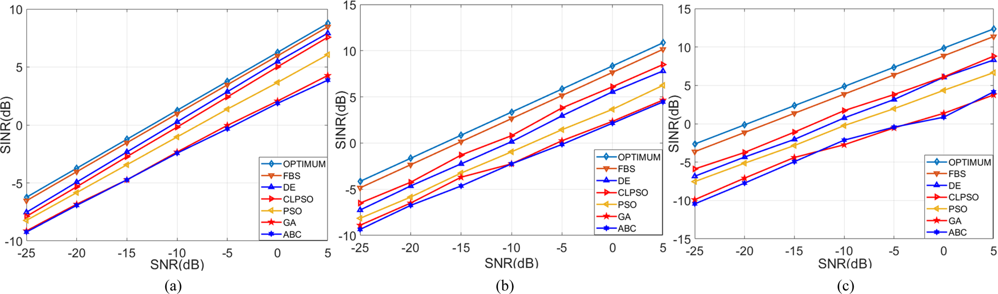
Simulation case one: four interference with 20 dB INR considered varied elements: The first case is two interference signals at 20 and 40° with 5 dB INR. The linear arrays are considered to be composed, respectively, of 6, 10, and 14 elements. The results of the output SINR are illustrated in Fig. 12. From the graphs, it can be noticed that the proposed algorithm outperforms the others for all the array element scenarios and is able to achieve near-optimal performance over the entire range of the input SNR values; CLPSO yields suboptimal higher values of SINR but FBS yields optimal SINR values consistently in all cases. Moreover, we can also observe that the performance difference in reaching optimum weight vectors between the FBS and other algorithms is increasing for the array element increment in each algorithm, this is consistent with previous results in section “Simulation case two: array element number investigation” owing to the increasing search dimension of the weight vectors solution in array element. With a view to the above fact, the global search capability of the proposed FBS algorithm could achieve the improvement of the output SINR more so than the compared metaheuristic-based beamformer in the adaptive beamformer system.
SINR performance versus SNR of the heuristic algorithms with varied array elements. (a) Six elements; (b) 10 elements; (c) 14 elements.

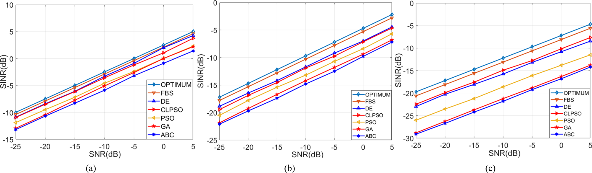
Simulation case two: four interference with different INR impinge on six-element array: A ULA consisting of six monochromatic isotropic elements receiving four interferences with different INR from respective 200, 400, 650, and −700 is considered in this scenario. Three groups of INRs of the interference set as 5, 20, 35 dB are established in different simulation scenarios. Figure 13 displays the SINR performance of these techniques versus the SNR under different power levels of interference sources by using the proposed and the compared optimization algorithms. From the results depicted in Fig. 13 we can know that, in general, the optimization algorithms are all able to achieve near-satisfactory SINR performance in the situation of INR = 5 dB, which means the lowest power process of the interference signal. The proposed algorithm achieved improved the performance in SINR than the other algorithms in all the simulations even under the most severe interference process when the value of INR is 30 dB. With the increasing of INR for the interference, the SINR performance of all the algorithms are degraded, and the proposed algorithms have evident advantages over these algorithms; therefore, note that the proposed algorithm can perform more robust results and suitable precisions in ABF for high interference power levels.
SINR performance versus SNR of the heuristic algorithms with different INR. (a) INR = 5 dB; (b) INR = 20 dB; (c) INR = 35 dB.

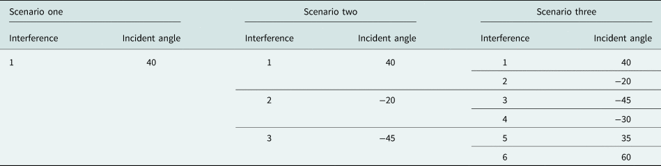
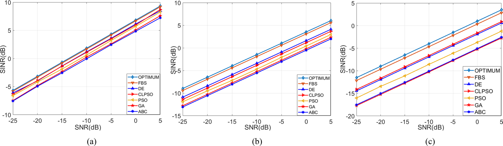
Simulation case three: different number of interferences with fixed INR received by six-element array: To prove the robustness of the proposed beamformer in this project, the simulations in this case were conducted to validate the effect of the interference quantity to the SINR performance, the beamformer is equipped with six array elements and the INR was fixed to 10 dB for the received interference signals, Table 9 illustrates the different number of interferences and the corresponding incident angle values of the above-mentioned interferences. The SINR performance of the proposed FBS and other optimization algorithms for different numbers of interference signals is shown in Fig. 14. As can be seen from Fig. 14, when there is one interference at the receiver, all the optimization algorithms can achieve the close-to-optimal SINR performance by considering the requirement for maximizing SINR, FBS demonstrates the best improvement, followed by DE. ABC shows the lowest value of SINR. As the number of interference increases from one to six, the superior performance advantage of the FBS becomes more evident. The increase in the number of interference sources increases the difficulty of the optimization problem. Failure of ABC, GA, and PSO to achieve sufficiently high SINR clearly illustrates their limitations; therefore, the proposed FBS is more versatile and robust than the other optimization methods in ABF application.
Different number of interferences for three scenarios

SINR performance versus SNR of the heuristic algorithms with a different number of interferences. (a) One interference; (b) three interferences; (c) six interferences.

Conclusions
In this paper, we presented a novel global optimization heuristic algorithm, called FBS, which is based on the use of the Fibonacci number series, to achieve the improved performance of the ABF. The interactive global and local searching rule was proposed to reduce the probability of falling into the local optima problem, and the global randomness characteristic and space region shortening fraction of this technique guarantee the convergence velocity in the global optimization process. Numerical multimodal benchmarking functions were employed to validate the effectiveness of these global optimization algorithms, and we found that generally FBS achieves a better convergence rate, precision, and stability compared to the others. In addition, we devise the specific implementation architecture based on FBS for adaptive beamformer; the amplitudes and phases of the weight vector acting as the solution were acquired in the search space by the FBS, and the beamforming results synthesized by the vectors were compared with conventional metaheuristic-based beamforming algorithms. The simulation experiments of section “Conclusions” demonstrate that the proposed beamforming method outperformed the compared methods significantly regarding the power beampattern and the output SINR for different scenarios. Consequently, the proposed FBS is a valuable tool for multi-objective optimization and well suited for ABF design problems, and it seems to be a quite promising smart antenna using beamforming technology. In the future work, the FBS will be explored to apply on a more complicated time-varying situation in ABF field.
 Haichuan Zhang was born in China in 1991. He received the Master’s degree in School of Electronic Countermeasures, National University of Defense Technology (NUDT), Hefei, China, in 2016. Since 2016, he proceeded with a doctoral research in the National University of Defense Technology. His research interests are in the areas of adaptive beamforming and its applications, array signal processing, and digital communication system.
 Fangling Zeng is currently a professor at the National University of Defense Technology (NUDT). She obtained her BSc, Master’s, and PhD degrees from the University of Science Technology (USTC) of China in 1996, 1999, and 2002, respectively. Her main research interests include precise point positioning phased array signal processing and GNSS/INS.