1 Introduction
Aeolian tone, caused by vortex shedding behind bluff bodies, has received continuous attention since the 1870s. It is well known that the frequency of Aeolian tone is always identical to the vortex shedding frequency, which varies linearly with the flow speed in free space. However, if a bluff body is placed in a confined space, such as a flow duct, the sound generation process becomes much more complicated due to the strong vortex sound interaction under certain conditions. This phenomenon is recognized as acoustic resonance, which is usually accompanied with a high intensity of tone. It causes severe noise pollution issues, as well as leading to performance deterioration or even catastrophic damage to the facility. These problems, undoubtedly, should be avoided in various military and civil engineering applications, such as combustion chambers of rockets (Karthik, Chakravarthy & Sujith Reference Karthik, Chakravarthy and Sujith2008), compressors of aero engines (Parker Reference Parker1968; Koch Reference Koch2009; Liu et al. Reference Liu, Willeke, Herbst, Yang and Sume2018), front grills of automobiles (Yokoyama, Kitamiya & Iida Reference Yokoyama, Kitamiya and Iida2013) and tube banks of heat exchangers (Mohany Reference Mohany2013; Shaaban & Mohany Reference Shaaban and Mohany2018). Consequently, the current research has been greatly motivated.
The general mechanism of acoustic resonance is usually described in the following manner. The boundary layer separates from a bluff body, forming an oscillating shear layer with inherent instability. If the fluctuation frequency of the shear layer coincides with that of an acoustic mode of the duct, the vortex shedding will be enhanced such that mutual capture starts, and a feedback loop can be sustained with the vortex shedding acting as the exciter and amplifier of the sound wave and the acoustic mode within the duct acting as the filter. Although the general process of acoustic resonance has been described by many authors, the underlying mechanism of vortex sound interaction is still an open issue.
Acoustic resonance in a duct induced by wake flow from an inner circular cylinder has been extensively studied since the 1950s, and the progress of research is summarized in some review papers (Blevins Reference Blevins1984; Mohany Reference Mohany2013; Ziada & Lafon Reference Ziada and Lafon2013). Through detailed flow visualization, the high correlation between the resonant sound and vortex shedding process has been substantiated. On the one hand, when an intense tone is excited, the vortex shedding becomes highly coherent in the streamwise direction and forms a succession of vortex clouds. On the other hand, if the wake flow is slightly disturbed by turbulent devices, such as smart rods, the acoustic resonance could be well eliminated (Katasonov, Sung & Bardakhanov Reference Katasonov, Sung and Bardakhanov2015). These observations have validated the role of vortex sound interaction in sustaining the acoustic resonance.
By means of large eddy simulation (known as LES) or direct numerical simulation (DNS), progress has been made on this issue, however, it is still a difficult problem to simulate the bi-directional coupling between vortex and sound in acoustic resonance, due to the large characteristic scale difference of the unsteady flow and acoustic motions. The DNS method, which directly solves the compressible Navier–Stokes equations, has advantages in describing the details of the sound and flow field, while the tremendous time consumption has become the limitation for practical applications. Yokoyama et al. (Reference Yokoyama, Kitamiya and Iida2013) studied the flow-induced acoustic resonance of a cascade of plate plates with DNS using 64 nodes (236.5 GFlops per node) in a supercomputer system, and 300 hours were needed for a single case with a very limited length of physical time; approximately 0.03 s. Therefore, it is difficult to give a continuous description from onset to exit of the lock-in phenomenon, which requires a relative long calculating time. For that reason, most of the previous investigations are based on decoupling methods, where the effect of feedback sound on vortex shedding is simulated through artificially introduced sound excitation (Tan, Thompson & Hourigan Reference Tan, Thompson and Hourigan2004; Mills, Sheridan & Hourigan Reference Mills, Sheridan and Hourigan2005; Mohany & Ziada Reference Mohany and Ziada2009; Mohany et al. Reference Mohany, Arthurs, Bolduc, Hassan and Ziada2014). These studies not only help in understanding the effect of sound on the behaviour of vortex shedding, but also can also give a qualitative analysis to the energy transfer between the flow field and the resonant sound field. As illustrated by Mohany & Ziada (Reference Mohany and Ziada2009), this is a one-way coupling where the feedback effect of resonant sound on the vortex shedding is accounted for, but the excitation of the sound field by the flow cannot be considered.
The question of what underlying mechanism dominates the frequency lock-in behaviour and the occurrence of peak amplitude in self-sustained acoustic resonance is of primary interest. It is commonly recognized that the onset of frequency lock-in will occur as soon as the vortex shedding frequency  $(f_{s})$ gets close to the inherent frequency of the acoustic
 $\unicode[STIX]{x1D6FD}$-mode
 $(f_{a})$. But the maximum resonant amplitude of acoustic resonance is not acquired at the synchronized point where the frequency ratio,
 $f_{s}/f_{a}$, exactly equals unity. It appears at a relative higher frequency ratio
 $(f_{s}/f_{a}>1)$. In this aspect, the acoustic resonance system cannot be simply considered to be a forced resonance system, the feedback effect of a sound wave on the vortex shedding is essential in the frequency lock-in procedure. To explore the underlying physical mechanism of frequency lock-in, a bi-directional simulation of the vortex sound interaction is necessary.
Numerically efficient theoretical modelling methods are particularly appealing tools for vortex sound interaction study in acoustic resonance. In this aspect, the discrete vortex method (DVM) has been extensively used, which is very suitable for the solution of shear layer separation in flows with high Reynolds number. Based on this method, the acoustic resonance and the vortex sound interaction behaviour of Helmholtz resonators are well depicted, and the predicted results of resonant amplitude and frequency are in good agreement with the experimental data (Hong et al. Reference Hong, Dai, Zhou, Sun and Jing2014; Dai, Jing & Sun Reference Dai, Jing and Sun2015; Dai Reference Dai2016). In Helmholtz resonators, the sound pressure can be conveniently related to the fluctuating velocity of the cavity opening through a lumped parameter model, as the sound source can be recognized to be compact. While for the cases of flow-induced acoustic resonance in flow ducts, the sound source becomes non-compact and the sound field must be solved separately with additional efforts. Langthjem & Nakano (Reference Langthjem and Nakano2005, Reference Langthjem and Nakano2013) established a mathematical model to study the flow-acoustic interaction in a hole-tone feedback system, where the unsteady shear layer is modelled via DVM and the sound field is modelled based on vortex sound theory. Besides, the acoustic particle velocity is superimposed onto the procedure of the vortex evolution to account for the feedback effect. This model gave reasonable results of the self-sustained oscillation, and illustrated the frequency lock-in phenomenon of the flow and resonant sound. These results show the possibility of exploring the underlying mechanism of frequency lock-in in acoustic resonance of flow ducts containing a circular cylinder.
Extensive experimental results reveal that the acoustic resonance is commonly excited by the vortex shedding with Reynolds numbers ranging from  $10^{4}$ to
 $10^{5}$ (Mohany & Ziada Reference Mohany and Ziada2009, Reference Mohany and Ziada2011; Arafa & Mohany Reference Arafa and Mohany2019; Shaaban & Mohany Reference Shaaban and Mohany2019). The wake flow behind the cylinder is essentially three-dimensional (3-D), however, during the acoustic resonance the wake flow becomes predominantly two-dimensional (2-D) as the vortex shedding along the spanwise direction is highly synchronized by the resonant sound (Blevins Reference Blevins1985; Mohany & Ziada Reference Mohany and Ziada2011). Therefore, a 2-D assumption is reasonable for the flow simulation in the acoustic resonance study, which can capture the flow physics well, as demonstrated by Mohany & Ziada (Reference Mohany and Ziada2009). As for the sound field within the duct, the acoustic resonance is initialized as soon as the vortex shedding frequency approaches the frequency of the first transverse acoustic mode (
 $\unicode[STIX]{x1D6FD}$-mode) of the duct. The frequency of this mode,
 $f_{a}$, can be approximately expressed as
 $f_{a}=c_{0}/2h$ (Mohany et al. Reference Mohany, Arthurs, Bolduc, Hassan and Ziada2014), where
 $c_{0}$ is the speed of sound wave and
 $h$ is the height of cross-section of the duct. From this aspect, a reasonable prediction of the frequency of the acoustic mode can be obtained with a 2-D flow duct assumption. So, 2-D flow and sound fields can be assumed to explore the frequency lock-in mechanism of the vortex sound interaction. However, 2-D methods usually over-predict the amplitude of sound pressure. To overcome the shortcoming of 2-D methods, a correction formula proposed by Oberai, Roknaldin & Hughes (Reference Oberai, Roknaldin and Hughes2002) has been extensively used to validate the accuracy of 2-D models with the measured results (Seo & Moon Reference Seo and Moon2007; Ewert et al. Reference Ewert, Appel, Dierke and Herr2009; Wu, Jing & Sun Reference Wu, Jing and Sun2017).
The main objective of the present work is to establish a nonlinear model that calculates the unsteady flow field, sound field and their bi-directional interaction simultaneously to explore the underlying mechanism of frequency lock-in in acoustic resonance. Firstly, the DVM is adopted to simulate the wake of a cylinder, and then a sub-model corresponding to the sound pressure radiated from vortex shedding is derived based on vortex sound theory. Next, the time domain boundary element method (TDBEM) is used to calculate the sound field within the duct, which considers the reflection and transmission effects of the rigid wall and the ends of the duct. In the end, the sound feedback effect is incorporated through adding acoustic particle velocity onto the Kutta condition of the vortex shedding to close the entire model. The published experimental data are used to validate the results of present model. Subsequently, the details of the underlying mechanism of frequency lock-in are explored in the following aspects: (i) a continuous frequency description of the onset–sustain–cease of acoustic resonance with varying flow velocities, (ii) the coupling regime of vortex and resonant sound and the underlying mechanism of frequency lock-in and (iii) the relation between the occurrence of maximum resonant sound pressure and the lock-in behaviour.
2 Modelling description
Assuming 2-D flow and acoustic fields, the present model consists of three components: a flow field model, a sound generation model and a sound propagation model. Moreover, the acoustic particle velocity is the link between the flow and sound fields, which close the feedback loop to capture the key features of the self-excited acoustic resonance. The 2-D assumption is valid for the frequency analysis of acoustic resonance, as the flow field is predominantly 2-D due to the sound modulation of the vortex shedding along the spanwise and the frequency of acoustic mode mainly depends on the height of the duct. However, the amplitudes of resonant tones would be inevitably over-estimated due to the limitation of the 2-D solution of sound field, therefore a 3-D correction method is introduced to validate the present sound pressure results by the published experimental data.
2.1 Discrete vortex method for the unsteady wake flow of a 2-D circular cylinder
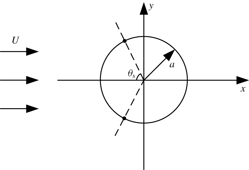
As shown in figure 1, a circular cylinder with a radius of  $a$ is immersed in the uniform flow with a velocity of
 $U$. The directions that are parallel and normal to the incoming flow are defined as
 $x$ and
 $y$, respectively, with the origin being fixed at the centre of the cylinder. The flow Mach number for present study is less than 0.3, so the incoming flow can be treated as incompressible.
Schematic diagram of the flow model.

The incoming flow is assumed to be irrotational except at the places where a point vortex locates, besides, a Kutta condition is applied at the two points where the vortices separated from the cylinder with a separation angel of  $\pm \unicode[STIX]{x1D703}_{s}$, as illustrated in figure 1. Since the flow field is assumed to be inviscid, the strength of the shed vortex should stay constant. However, an attenuation function is used to artificially simulate the viscous effect, which is expressed as (Kiya, Sasaki & Arie Reference Kiya, Sasaki and Arie1982)
 $$\begin{eqnarray}\frac{\unicode[STIX]{x1D6E4}(t)}{\unicode[STIX]{x1D6E4}_{0}}=1-\exp \left(-\frac{A^{2}Re}{4(Ut)/a}\right),\end{eqnarray}$$
where  $\unicode[STIX]{x1D6E4}_{0}$ is the initial strength of a point vortex,
 $\unicode[STIX]{x1D6E4}(t)$ is the strength of a point vortex at time
 $t$,
 $A$ is an empirical number and
 $Re$ is the Reynolds number based on the diameter of the cylinder
 $d$. Accordingly,
 $A^{2}Re$ is a constant which merely relates to the type of the incoming flow, and it is set to 32 here, based on plenty of numerical trials.
The complex velocity of the flow field,  $\boldsymbol{w}(\boldsymbol{z})$, includes three components: the uniform flow, the doublet at the centre of the cylinder and the point vortices and their images. Its expression is written as
 $$\begin{eqnarray}\boldsymbol{w}(\boldsymbol{z})=U-\frac{Ua^{2}}{\boldsymbol{z}^{2}}+\frac{1}{2\unicode[STIX]{x03C0}\text{i}}\mathop{\sum }_{n=1}^{N_{v}}\left[\frac{\unicode[STIX]{x1D6E4}_{n}}{\boldsymbol{z}-\boldsymbol{z}_{n}}-\frac{\unicode[STIX]{x1D6E4}_{n}}{\boldsymbol{z}-a^{2}/\overline{\boldsymbol{z}}_{n}}\right],\end{eqnarray}$$
where  $N_{v}$ is the total number of point vortices in the wake. It should be mentioned that in order to satisfy the rigid wall condition on the cylinder surface, the complex potential is obtained by placing an image vortex with a strength of
 $-\unicode[STIX]{x1D6E4}_{n}$ at the point
 $\boldsymbol{z}=a^{2}/\overline{\boldsymbol{z}}_{n}$, where the bar denotes the complex conjugate. Besides, the image vortex at the centre of the cylinder is removed to ensure that the total circulation in the whole domain vanishes. When solving the velocity of the
 $n$th point vortex
 $\boldsymbol{w}(\boldsymbol{z}_{n})$, the velocity induced by itself should be subtracted and then the velocity expression becomes
 $$\begin{eqnarray}\boldsymbol{w}(\boldsymbol{z}_{n})=U-\frac{Ua^{2}}{\boldsymbol{z}_{n}^{2}}+\frac{1}{2\unicode[STIX]{x03C0}\text{i}}\mathop{\sum }_{\substack{ n^{\prime }=1 \\ n^{\prime }\neq n}}^{N_{v}}\left[\frac{\unicode[STIX]{x1D6E4}_{n^{\prime }}}{\boldsymbol{z}-\boldsymbol{z}_{n^{\prime }}}-\frac{\unicode[STIX]{x1D6E4}_{n^{\prime }}}{\boldsymbol{z}-a^{2}/\overline{\boldsymbol{z}}_{n^{\prime }}}\right].\end{eqnarray}$$
After a point vortex is shed into the flow field, its trajectory can be calculated by solving the following ordinary differential equations
 $$\begin{eqnarray}\frac{\text{d}\boldsymbol{z}_{n}}{\text{d}t}=\boldsymbol{w}(\boldsymbol{z}_{n}),\end{eqnarray}$$
where  $\boldsymbol{z}_{n}$ is the complex coordinate of the
 $n$th point vortex.
As is known, the separation points on a cylinder oscillate periodically with a small amplitude due to the influence from the wake. Although they can be numerically determined using the integral boundary layer equations, this is quite complex and numerical instability is often encountered due to the mathematical properties of these equations. Fortunately, reasonable results can be obtained if a simpler assumption is made of fixed separation points (Ramos-García et al. Reference Ramos-García, Sarlak, Andersen and Sørensen2017). It is commonly accepted that the separation angle of the flow past a cylinder depends on the Reynolds number. As summarized by Schlichting & Gersten (Reference Schlichting and Gersten2017), in the subcritical Reynolds number region  $(300<Re<1.3\times 10^{5})$, the separation angle is approximately
 $80^{\circ }$. As mentioned above, the Reynolds number relevant to acoustic resonance usually falls in the interval
 $10^{4}<Re<10^{5}$, thus the vortex shedding behind the cylinder belongs to a subcritical flow with a laminar boundary layer. According to the experimental measurements of Achenbach (Schlichting & Gersten Reference Schlichting and Gersten2017), the two separation points locate at an angle of
 $\unicode[STIX]{x1D703}_{s}\approx \pm 78^{\circ }$ from the front stagnation point in the subcritical flows. The results based on DVM by Sarpkaya & Schoaff (Reference Sarpkaya and Schoaff1979) also show that the mean position of the separation point locates at
 $\unicode[STIX]{x1D703}_{s}\approx 78^{\circ }$. So, in this study, a separation angel of
 $78^{\circ }$ is chosen following the numerical results of Sarpkaya & Schoaff (Reference Sarpkaya and Schoaff1979) and the experimental data of Achenbach (Schlichting & Gersten Reference Schlichting and Gersten2017). Furthermore, the numerical experiments prove that the flow field results of the present model are not sensitive to the delicate difference of the separation angle ranges from
 $78^{\circ }$ to
 $80^{\circ }$.
At the beginning of each time step, only one point vortex is shed from the upper and lower separation point, respectively, with the strength  $\unicode[STIX]{x1D6E4}_{nv}$ being determined by
 $$\begin{eqnarray}\unicode[STIX]{x1D6E4}_{nv}=0.5U_{s}^{2}\unicode[STIX]{x0394}t,\end{eqnarray}$$
where  $U_{s}$ is the outer velocity of the boundary layer at the separation point, and the thickness of the boundary layer,
 $\unicode[STIX]{x1D6FF}$, is set at
 $0.02a$, a typical value for a circular cylinder in subcritical flows (Schlichting & Gersten Reference Schlichting and Gersten2017). The position of the nascent vortex is determined by applying non-slip conditions at the separation point, which can be expressed as (Sarpkaya & Schoaff Reference Sarpkaya and Schoaff1979)
 $$\begin{eqnarray}\boldsymbol{z}_{nv}^{j}=a\left[\frac{1+|\unicode[STIX]{x1D6E4}_{nv}^{j}|/(2\unicode[STIX]{x03C0}U_{s}^{j}a)}{1-|\unicode[STIX]{x1D6E4}_{nv}^{j}|/(2\unicode[STIX]{x03C0}U_{s}^{j}a)}\right]\exp [\text{i}(\unicode[STIX]{x03C0}-\unicode[STIX]{x1D703}_{s}^{j})],\end{eqnarray}$$
where  $j$ represents 1 or 2 corresponding to the upper or lower nascent point vortex.
The aerodynamic force exerted on the cylinder can be derived from the generalized Blasius theorem, which is expressed as (Sarpkaya & Schoaff Reference Sarpkaya and Schoaff1979)
 $$\begin{eqnarray}C_{D}+\text{i}C_{L}=\text{i}\frac{\unicode[STIX]{x2202}}{\unicode[STIX]{x2202}t}\mathop{\sum }_{n=1}^{N_{v}}\unicode[STIX]{x1D6E4}_{n}(\boldsymbol{z}_{n}-a^{2}/\overline{\boldsymbol{z}}_{n}),\end{eqnarray}$$
where  $C_{D}$ and
 $C_{L}$ are the drag and lift coefficients, respectively.
2.2 Vortex sound theory for sound radiation from the vortex shedding within the duct
In a low Mach number, isentropic and inviscid flow field, the sound wave equation can be expressed as (Howe Reference Howe2003)
 $$\begin{eqnarray}\left(\frac{1}{c_{0}^{2}}\frac{\unicode[STIX]{x2202}^{2}}{\unicode[STIX]{x2202}t^{2}}-\unicode[STIX]{x1D6FB}^{2}\right)\frac{p}{\unicode[STIX]{x1D70C}_{0}}=\unicode[STIX]{x1D735}\boldsymbol{\cdot }(\unicode[STIX]{x1D74E}\times \boldsymbol{v}),\end{eqnarray}$$
where  $p$ is the sound pressure,
 $\unicode[STIX]{x1D70C}_{0}$ is the ambient far-field density,
 $\unicode[STIX]{x1D74E}$ and
 $\boldsymbol{v}$ represent the rotation and convection velocity of the vortex, respectively.
In a 2-D free space, the general solution of sound pressure induced by a vortex can be obtained by means of the Green’s function. The sound pressure radiated from the  $n$th point vortex,
 $p_{n}$, is written as
 $$\begin{eqnarray}\frac{p_{n}}{\unicode[STIX]{x1D70C}_{0}}=\int _{0}^{t}\int _{\unicode[STIX]{x1D6FA}}\unicode[STIX]{x1D735}\boldsymbol{\cdot }(\unicode[STIX]{x1D74E}_{n}\times \boldsymbol{v}_{n})G\,\text{d}\unicode[STIX]{x1D6FA}\,\text{d}\unicode[STIX]{x1D70F}=-\int _{0}^{t}\int _{\unicode[STIX]{x1D6FA}}(\unicode[STIX]{x1D74E}_{n}\times \boldsymbol{v}_{n})\boldsymbol{\cdot }\unicode[STIX]{x1D735}G\,\text{d}\unicode[STIX]{x1D6FA}\,\text{d}\unicode[STIX]{x1D70F},\end{eqnarray}$$
where  $\unicode[STIX]{x1D6FA}$ denotes the control surface element,
 $\unicode[STIX]{x1D74E}_{n}$ and
 $\boldsymbol{v}_{n}$ are the rotation and convection velocity of the
 $n$th vortex,
 $\unicode[STIX]{x1D74E}_{n}=\boldsymbol{k}\unicode[STIX]{x1D6E4}_{n}\unicode[STIX]{x1D6FF}(y_{1}-y_{1n}(\unicode[STIX]{x1D70F}))(y_{2}-y_{2n}(\unicode[STIX]{x1D70F}))$,
 $\boldsymbol{v}_{n}=\boldsymbol{i}u_{n}+\boldsymbol{j}v_{n}$, and
 $G$ is the 2-D free space Green’s function in the time domain, expressed as
 $$\begin{eqnarray}G(\boldsymbol{x},t/\boldsymbol{y},\unicode[STIX]{x1D70F})=\frac{c_{0}H[c_{0}(t-\unicode[STIX]{x1D70F})-R]}{2\unicode[STIX]{x03C0}\sqrt{c_{0}^{2}(t-\unicode[STIX]{x1D70F})^{2}-R^{2}}},\end{eqnarray}$$
where  $\boldsymbol{x}\,(x_{1},x_{2})$ and
 $\boldsymbol{y}\,(y_{1},y_{2})$ denote the coordinates of observation and source points with a distance of
 $R$ between them,
 $t$ and
 $\unicode[STIX]{x1D70F}$ represent the observation and release time, respectively, and
 $H$ is the Heaviside function. After a series of derivations as presented in appendix A, the sound pressure radiated from the
 $n$th vortex can be depicted as
 $$\begin{eqnarray}\left.\begin{array}{@{}c@{}}\displaystyle \frac{p_{n}}{\unicode[STIX]{x1D70C}_{0}}=\int _{0}^{t}\left(XB+\frac{\unicode[STIX]{x2202}X}{\unicode[STIX]{x2202}\unicode[STIX]{x1D70F}}\frac{G}{c_{0}}\right)\,\text{d}\unicode[STIX]{x1D70F},\\ \displaystyle X=\unicode[STIX]{x1D6E4}_{n}\left(u_{n}\frac{\unicode[STIX]{x2202}R}{\unicode[STIX]{x2202}y_{2}}-v_{n}\frac{\unicode[STIX]{x2202}R}{\unicode[STIX]{x2202}y_{1}}\right),\quad B=\frac{c_{0}[c_{0}(t-\unicode[STIX]{x1D70F})-R]H[c_{0}(t-\unicode[STIX]{x1D70F})-R]}{2\unicode[STIX]{x03C0}\sqrt{[c_{0}^{2}(t-\unicode[STIX]{x1D70F})^{2}-R^{2}]^{3}}}.\end{array}\right\}\end{eqnarray}$$
The total sound pressure radiated from the wake flow that contains  $N_{v}$ vortices is written as
 $$\begin{eqnarray}p=\mathop{\sum }_{n=1}^{N_{v}}p_{n}.\end{eqnarray}$$
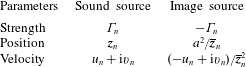
As described in the above section, the free space Green’s function is chosen for the solution of sound generation, which means the reflection effects of the cylinder surface should be taken into consideration during the sound propagation. In this respect, the image theory is adopted, which means the presence of the rigid wall is accounted for by introducing image sound sources. The parameters of the sound source (the  $n$th point vortex) and its image have been conveniently obtained in the flow field simulation by DVM, as shown in table 1.
Parameters of the sound source and its image.

The integral expression of the sound wave equation in the 2-D duct containing  $N_{v}$ vortices can be written as (Aliabadi & Wen Reference Aliabadi and Wen2010)
 $$\begin{eqnarray}\unicode[STIX]{x1D70D}(Q)p(Q,t)=\int _{0}^{t}\int _{\unicode[STIX]{x1D6F1}}\left(G\frac{\unicode[STIX]{x2202}p}{\unicode[STIX]{x2202}\boldsymbol{n}}-p\frac{\unicode[STIX]{x2202}G}{\unicode[STIX]{x2202}\boldsymbol{n}}\right)\,\text{d}\unicode[STIX]{x1D6F1}\,\text{d}\unicode[STIX]{x1D70F}+S,\end{eqnarray}$$
where  $\unicode[STIX]{x1D6F1}$ represents the boundary of the duct,
 $S$ represents the sound source generated by the vortices within the duct and
 $\boldsymbol{n}$ is the identity normal vector. Here
 $\unicode[STIX]{x1D70D}(Q)$ is a constant number related to the positions of
 $Q$, such that
 $$\begin{eqnarray}\unicode[STIX]{x1D70D}(Q)=\left\{\begin{array}{@{}ll@{}}1 & Q\in \unicode[STIX]{x1D6FA}\\ 1/2 & Q\in \unicode[STIX]{x1D6F1}\\ 0 & Q\notin \unicode[STIX]{x1D6FA}.\end{array}\right.\end{eqnarray}$$
Substituting (2.10) into (2.13), the following equation is obtained; the derivation is similar to the TDBEM derived by Mansur et al. (Aliabadi & Wen Reference Aliabadi and Wen2010),
 $$\begin{eqnarray}\unicode[STIX]{x1D70D}(Q)p(Q,t)=\int _{0}^{t}\int _{\unicode[STIX]{x1D6F1}}bG\,\text{d}\unicode[STIX]{x1D6F1}\,\text{d}\unicode[STIX]{x1D70F}+\int _{0}^{t}\int _{\unicode[STIX]{x1D6F1}}\frac{\unicode[STIX]{x2202}R}{\unicode[STIX]{x2202}\boldsymbol{n}}\left(pB+\frac{\unicode[STIX]{x2202}p}{\unicode[STIX]{x2202}\unicode[STIX]{x1D70F}}\frac{G}{c_{0}}\right)\,\text{d}\unicode[STIX]{x1D6F1}\,\text{d}\unicode[STIX]{x1D70F}+\sum S,\end{eqnarray}$$
where  $b=\unicode[STIX]{x2202}p(Q,t)/\unicode[STIX]{x2202}\boldsymbol{n}$.
2.3 Modelling of acoustic feedback
According to the experimental results measured by Blevins (Reference Blevins1985), the sound wave affects the flow field through the feedback of the acoustic particle velocity. In the present model, the acoustic particle velocity at the separation point is solved based on the sound pressure results. Then it is added to the complex velocity of the flow field to determine the outer velocity of the boundary layer at the separation point through the Kutta condition, which can be expressed as
 $$\begin{eqnarray}U_{s}=U-\frac{Ua^{2}}{\boldsymbol{z}_{s}^{2}}+\frac{1}{2\unicode[STIX]{x1D70B}\text{i}}\mathop{\sum }_{n=1}^{N_{v}}\left[\frac{\unicode[STIX]{x1D6E4}_{n}}{\boldsymbol{z}_{s}-\boldsymbol{z}_{n}}-\frac{\unicode[STIX]{x1D6E4}_{n}}{\boldsymbol{z}_{s}-a^{2}/\overline{\boldsymbol{z}}_{n}}\right]+u_{a},\end{eqnarray}$$
where  $\boldsymbol{z}_{s}$,
 $\boldsymbol{z}_{s}=a(1+\unicode[STIX]{x1D6FF})\exp [\text{i}(\unicode[STIX]{x03C0}-\unicode[STIX]{x1D703}_{s})]$, represents the position where the nascent vortex is introduced into the flow field. As the sound pressure within the duct has been obtained according to (2.15), then it can readily be used to determine the acoustic particle velocity through numerically solving the momentum equation, written as
 $$\begin{eqnarray}u_{a}=-\frac{1}{\unicode[STIX]{x1D70C}_{0}}\int \frac{\unicode[STIX]{x2202}p}{\unicode[STIX]{x2202}x}\,\text{d}t.\end{eqnarray}$$
After the acoustic feedback effect is taken into consideration, the coupling loop between vortex and sound has been closed. Although the flow field and sound field are solved by separate governing equations, the two fields and their interaction can be solved simultaneously within the same time step and no spatial or temporal interpolation is needed as all the models are based on time-domain meshless methods. In this aspect, the present method may be classified into the catalogue of strong coupling methods, which is the essential difference between the present model and the decoupling methods that were mentioned before in § 1.
2.4 Correction of sound pressure using a 2-D to 3-D scaling technique
To compare the 2-D sound pressure results with the experimental data, a 2-D to 3-D scaling technique proposed by Ewert et al. (Reference Ewert, Appel, Dierke and Herr2009), a modified form of Oberai’s formula, is employed in the present model. The 3-D sound pressure in the frequency domain,  $\hat{p}_{3D}$, is related to the 2-D predicted results,
 $\hat{p}_{2D}$, by the following expression
 $$\begin{eqnarray}\hat{p}_{3D}=\frac{1+\text{i}}{2}\sqrt{\frac{k}{2\unicode[STIX]{x03C0}R}}\hat{L}_{z}\hat{p}_{2D},\end{eqnarray}$$
where  $k$ is the wavenumber of sound and
 $\hat{L}_{z}$ is the spanwise coherence length, which relates to the frequency of the sound pressure. The value of
 $\hat{L}_{z}$ at the fundamental frequency of the vortex shedding is set to be
 $6d$, according to Seo & Moon (Reference Seo and Moon2007).
The above formula is derived in the frequency domain, so it is used as a post-processing method after the 2-D sound spectra are obtained using the fast Fourier transformation (FFT).
3 Numerical implementation
3.1 Vortex shedding from the cylinder
A typical time marching approach of flow field solution using DVM is implemented in the following four steps:
(1) The positions of nascent vortices shed from the upper and lower separation point at the start of time step
 $m$ are determined by (2.6).
(2) Assign the circulations of nascent vortices through (2.5), and then evaluate the strengths of previous vortices using (2.1).
(3) Update the positions of previous vortices existing in the flow field by solving (2.4) through the fourth-order Runge–Kutta method.
(4) Increase the time step
$t_{m+1}=t_{m}+\unicode[STIX]{x0394}t$, and then repeat the above three steps.


It should be stated that, the wake flow consisting of point vortices is smoothed by assuming a Rankine vortex velocity field within a distance of  $\unicode[STIX]{x1D705}e$ from their centres, where
 $\unicode[STIX]{x1D705}$ is a constant smaller than unity and
 $e$ is the length of the feeding sheet of the nascent vortex. In this simulation the value of
 $\unicode[STIX]{x1D705}$ is selected to be 0.8, and the results are not sensitive to the choice of
 $\unicode[STIX]{x1D705}$, verified by plenty of previous research (Dai, Jing & Sun Reference Dai, Jing and Sun2012; Hong et al. Reference Hong, Dai, Zhou, Sun and Jing2014). With the increase of time steps and the number of vortices in the flow field, the computational cost becomes larger and larger. Therefore, we employ special treatments to keep the computational expense within acceptable bounds. Firstly, the strengths of the vortices are gradually attenuated through (2.1), which means the vortices gradually decrease in strength under the action of artificial viscosity when being convected downstream. Subsequently, the effects of the vortices blown far away from the cylinder are reasonably truncated at a certain distance of
 $30d$, following the numerical model of Inoue & Hatakeyama (Reference Inoue and Hatakeyama2002).
3.2 Sound wave propagation within the duct
The conventional collocation method (Aliabadi & Wen Reference Aliabadi and Wen2010) is employed to discretize the boundary integral equation (2.15), in which the boundary,  $\unicode[STIX]{x1D6F1}$, is represented by a set of discrete nodes
 $Q_{j}$,
 $j=1,2,3,\ldots ,J$, and the time is discretized into equal intervals
 $[t_{n},t_{n+1}]\;n=1,2,3,\ldots ,N$. Then,
 $p(Q,t)$ and
 $b(Q,t)$ can be approximated by using a set of interpolation functions as illustrated below
 $$\begin{eqnarray}\left.\begin{array}{@{}c@{}}\displaystyle p(Q,t)=\mathop{\sum }_{j=1}^{J}\mathop{\sum }_{m=1}^{N}\unicode[STIX]{x1D711}^{m}(t)\unicode[STIX]{x1D702}_{j}(Q)p_{j}^{m}=\mathop{\sum }_{j=1}^{J}\mathop{\sum }_{m=1}^{N}\unicode[STIX]{x1D711}^{m}(t)\unicode[STIX]{x1D702}_{j}(Q)p(Q_{j},t_{m})\\ \displaystyle b(Q,t)=\mathop{\sum }_{j=1}^{J}\mathop{\sum }_{m=1}^{N}\unicode[STIX]{x1D703}^{m}(t)\unicode[STIX]{x1D701}_{j}(Q)b_{j}^{m}=\mathop{\sum }_{j=1}^{J}\mathop{\sum }_{m=1}^{N}\unicode[STIX]{x1D703}^{m}(t)\unicode[STIX]{x1D701}_{j}(Q)b(Q_{j},t_{m}),\end{array}\right\}\end{eqnarray}$$
where  $m$ and
 $j$ refer to the time and space variations, respectively, and
 $\unicode[STIX]{x1D702}_{j}$,
 $\unicode[STIX]{x1D701}_{j}$,
 $\unicode[STIX]{x1D711}^{m}$ and
 $\unicode[STIX]{x1D703}^{m}$ are interpolation functions with respect to node
 $j$ and time interval
 $m$, expressed as (Aliabadi & Wen Reference Aliabadi and Wen2010)
 $$\begin{eqnarray}\left.\begin{array}{@{}c@{}}\displaystyle \unicode[STIX]{x1D711}^{m}(\unicode[STIX]{x1D70F})=\left\{\begin{array}{@{}ll@{}}(\unicode[STIX]{x1D70F}-t_{m-1})/\unicode[STIX]{x0394}t & t_{m-1}<\unicode[STIX]{x1D70F}\leqslant t_{m},\\ (t_{m+1}-\unicode[STIX]{x1D70F})/\unicode[STIX]{x0394}t & t_{m}<\unicode[STIX]{x1D70F}\leqslant t_{m+1},\\ 0 & \text{otherwise},\end{array}\right.\quad \unicode[STIX]{x1D703}^{m}(\unicode[STIX]{x1D70F})=\left\{\begin{array}{@{}ll@{}}1 & t_{m-1}\leqslant \unicode[STIX]{x1D70F}\leqslant t_{m},\\ 0 & \text{otherwise},\end{array}\right.\\ \displaystyle \unicode[STIX]{x1D702}_{j}(\unicode[STIX]{x1D709})=\unicode[STIX]{x1D701}_{j}(\unicode[STIX]{x1D709})=\left\{\begin{array}{@{}ll@{}}\displaystyle (\unicode[STIX]{x1D709}_{p}+1)/2 & Q\in e_{p},\\ -(\unicode[STIX]{x1D709}_{q}-1)/2 & Q\in e_{q},\\ 0 & \text{otherwise},\end{array}\right.\end{array}\right\}\end{eqnarray}$$
where  $\unicode[STIX]{x1D709}$ represents the coordinate along the boundary element,
 $e_{p}$ and
 $e_{q}$ are the adjacent elements with a common node. Based on the above discretization, the time integration in (2.15) can be readily implemented, and is written as
 $$\begin{eqnarray}\unicode[STIX]{x1D70D}p_{i}^{n}-\mathop{\sum }_{j=1}^{J}\mathop{\sum }_{m=1}^{N}D_{ij}^{nm}p_{j}^{m}-\mathop{\sum }_{j=1}^{J}\mathop{\sum }_{m=1}^{N}E_{ij}^{nm}b_{j}^{m}=S_{i}^{n}.\end{eqnarray}$$
In the above equation,  $n$ and
 $i$ represent the variations of
 $n$th boundary element at the
 $i$th time step,
 $D_{ij}^{nm}$ and
 $E_{ij}^{nm}$ are coefficients resulting from the temporal integration, which are defined as follows
 $$\begin{eqnarray}D_{ij}^{nm}=\int _{\unicode[STIX]{x1D6F1}}\frac{\unicode[STIX]{x2202}R}{\unicode[STIX]{x2202}\boldsymbol{n}}\unicode[STIX]{x1D702}_{j}(\unicode[STIX]{x1D709})Y^{nm}\,\text{d}\unicode[STIX]{x1D6F1},\quad E_{ij}^{nm}=\int _{\unicode[STIX]{x1D6F1}}\unicode[STIX]{x1D701}_{j}(\unicode[STIX]{x1D709})T^{nm}\,\text{d}\unicode[STIX]{x1D6F1},\end{eqnarray}$$
where
 $$\begin{eqnarray}Y^{nm}=\int _{0}^{t_{n}}\left[\unicode[STIX]{x1D711}^{m}(\unicode[STIX]{x1D70F})B+\frac{1}{c_{0}}\frac{\unicode[STIX]{x2202}\unicode[STIX]{x1D711}^{m}(\unicode[STIX]{x1D70F})}{\unicode[STIX]{x2202}\unicode[STIX]{x1D70F}}G\right]\,\text{d}\unicode[STIX]{x1D70F},\quad T^{nm}=\int _{0}^{t_{n}}\unicode[STIX]{x1D703}^{m}(\unicode[STIX]{x1D70F})G\,\text{d}\unicode[STIX]{x1D70F}.\end{eqnarray}$$
The values of  $Y^{nm}$ and
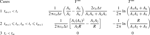
 $T^{nm}$ depend on the positions of the sound wave front, which can be described by the following cases as shown in table 2.
Time integrated kernels.
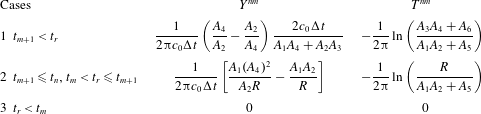
The relative variables in the table 2 are defined as
 $$\begin{eqnarray}\left.\begin{array}{@{}c@{}}\displaystyle A_{1,2}=\sqrt{c_{0}(t_{n}-t_{m})\mp R},\quad A_{3,4}=\sqrt{c_{0}(t_{n}-t_{m+1})\mp R},\quad A_{5}=c_{0}(t_{n}-t_{m}),\\ \displaystyle A_{6}=c_{0}(t_{n}-t_{m+1}),\quad t_{r}=t_{n}-R/c_{0}.\end{array}\right\}\end{eqnarray}$$
After the time integrations are determined, Gauss quadrature is employed to implement the spatial integration in (3.4). Finally, the sound pressure at any position within the duct at time  $t_{n}$ can be obtained from solving (3.3).
Note that, the numerical instability issue of TDBEM would eventually restrict the effective time length of the calculation. Owing to a variety of elaborate work that tries to solve the problem, the instability can be alleviated to some extent (Carrer, Pereira & Mansur Reference Carrer, Pereira and Mansur2012; Jang & Ih Reference Jang and Ih2012). In the present model, the instability problem in TDBEM is simply alleviated by properly choosing the time step,  $\unicode[STIX]{x0394}t$, and the length of boundary element,
 $l_{e}$, for convenience. A non-dimensional parameter
 $\unicode[STIX]{x1D6FC}$ is usually used for the choice of
 $\unicode[STIX]{x0394}t$ and
 $l_{e}$;
 $$\begin{eqnarray}\unicode[STIX]{x1D6FC}=\frac{c_{0}\unicode[STIX]{x0394}t}{l_{e}}.\end{eqnarray}$$
It is recommended that the value of  $\unicode[STIX]{x1D6FC}$ should fall in the interval
 $0<\unicode[STIX]{x1D6FC}<1.0$ and avoid too small or large values (Carrer, Pereira & Mansur Reference Carrer, Pereira and Mansur2012).
3.3 Sound pressure radiation from the vortex shedding
The calculation of wake flow behind the cylinder gives the positions, strengths and velocities of all the vortices in the flow field, so it is convenient to evaluate the sound pressure through (2.11) and (2.12). However, it is a difficult task to solve these integral equations through pure numerical methods due to the ‘tail effect’ of the 2-D Green’s function in the time domain. This means the effect of the sound wave radiated from one instant of time may theoretically last to infinity, which is computationally expensive for the numerical integration methods. For this reason, some analytical operations are preferred here. It is straightforward to find that the time integral in (2.11) has the same form as that of the second term on the right-hand side of (2.15). The above two time integrals are expressed as  $\int _{0}^{t}X(B+G/c_{0}\cdot \unicode[STIX]{x2202}/\unicode[STIX]{x2202}\unicode[STIX]{x1D70F})\,\text{d}\unicode[STIX]{x1D70F}$ and
 $\int _{0}^{t}p(B+G/c_{0}\cdot \unicode[STIX]{x2202}/\unicode[STIX]{x2202}\unicode[STIX]{x1D70F})\,\text{d}\unicode[STIX]{x1D70F}$, respectively. Therefore, (2.11) can be semi-analytically solved with the same discretization procedure in the time integration of TDBEM as shown in (3.4) (see the expression of
 $Y^{nm}$). The sound pressure radiated from the vortex can be approximated by using linear interpolation function, which is written as
 $$\begin{eqnarray}S_{i}^{n}=\mathop{\sum }_{m=1}^{N}Y^{nm}X^{m}.\end{eqnarray}$$
4 Results and discussions
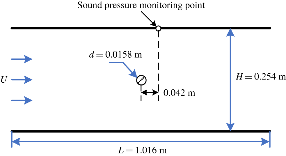
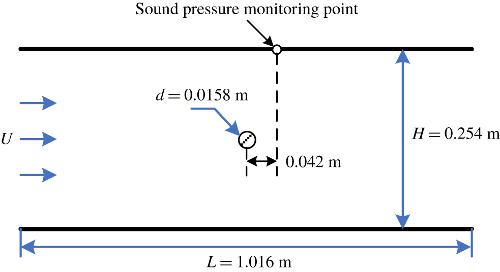
To verify the present model, the dimensions of the computational domain and the position of the observation point are the same as the previous experimental work of Mohany & Ziada (Reference Mohany and Ziada2011), as shown in figure 2. A circular cylinder, with a diameter of 0.0158 m, is placed on the centre line of a flow duct with dimensions of  $L=1.016~\text{m}$ in length and
 $H=0.254~\text{m}$ in height. As the blockage ratio of the cylinder to the duct is quite low, the effect of the duct wall on the vortex shedding can be ignored. The density of inner flow is
 $\unicode[STIX]{x1D70C}=1.225~\text{kg}~\text{m}^{-3}$ and the viscosity is
 $\unicode[STIX]{x1D707}=1.7894\times 10^{-5}~\text{Pa}~\text{s}$. The velocity of incoming uniform flow varies from
 $40~\text{m}~\text{s}^{-1}$ to
 $75~\text{m}~\text{s}^{-1}$, which results in a range of Reynolds number between
 $4.3\times 10^{4}$ and
 $8.1\times 10^{4}$.
Many preliminary runs have been carried out to choose the values of time step  $\unicode[STIX]{x0394}t$ and the length of boundary element
 $l_{e}$ to obtain stable results for flow and sound fields. It is found that the following combination of parameters,
 $\unicode[STIX]{x0394}t=0.08a/U$,
 $l_{e}\approx c_{0}\unicode[STIX]{x0394}t/0.6$, render stable results with sufficient accuracy and acceptable time expense. In this manner, the value of the non-dimensional parameter,
 $\unicode[STIX]{x1D6FC}$ in (3.7), is approximately 0.6, which agrees well with the findings of Carrer et al. (Reference Carrer, Pereira and Mansur2012). Moreover, as the reflection of the sound wave by the opening duct ends can be neglected, only boundary discretization on the duct-wall is necessary, and two auxiliary elements are added at each duct opening to enclose the whole boundary for the interior sound propagation calculation. Accordingly, the total number of boundary elements ranges from 238 to 428 corresponding to the flow velocity interval,
 $40~\text{m}~\text{s}^{-1}<U<75~\text{m}~\text{s}^{-1}$.
The rigid-wall boundary conditions are conveniently applied on the duct walls to account for the sound wave reflection. As the TDBEM satisfies the far field radiation condition automatically, where the sound wave can freely propagate out of the duct ends, therefore non-reflection boundary conditions are not necessary in this simulation, which further reduces the computational expense.
Sketch of the flow duct containing a circular cylinder.
Note that all the following results are non-dimensionalized. The distance and physical time are normalized by the diameter of cylinder  $d$ and
 $d/U$, respectively. The strength of vortex is normalized by
 $Ud$, the reduced velocity and frequency are defined as
 $U_{r}=U/f_{a}d$ and
 $f_{r}=f/f_{a}$, respectively, the normalized sound pressure is given by
 $p^{\ast }=p/(0.5\unicode[STIX]{x1D70C}U^{2}M)$ (Mohany & Ziada Reference Mohany and Ziada2011) and
 $M$ represents the Mach number.
4.1 Flow field results
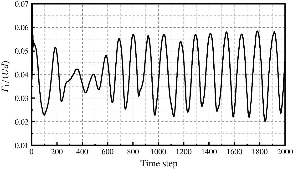
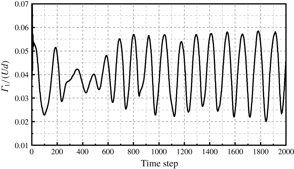
The flow field results in free space are illustrated in this section to explore the natural shedding frequency of the wake flow. A total number of 34 000 steps are implemented, which require approximately 3 central processing unit (CPU) hours. The last 32 768 steps are analysed using FFT with the initial 1232 steps being discarded as transient data. The flow field has already fully developed to a typical periodic oscillating state after approximately 900 steps, as shown by the time history of strength of nascent vortex for  $U_{r}=5.06$ in figure 3.
Time history of the strength of nascent point vortex.
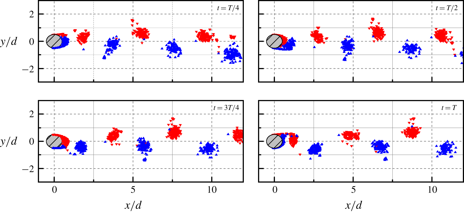
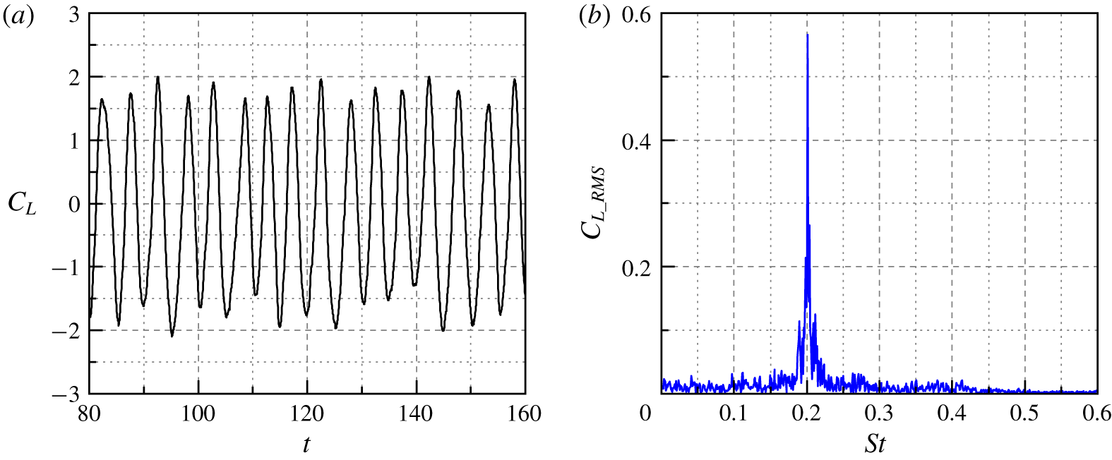
A representative result of the flow structure behind the cylinder during an arbitrary period is shown in figure 4, where the Kármán vortex street is clearly visible. The time history of the lift coefficient  $(C_{L})$ for a reduced velocity of
 $U_{r}=5.06$ is shown in figure 5(a). From the spectrum shown in figure 4(b), it demonstrates that the Strouhal number of the vortex shedding is
 $St\approx 0.2$, and the root mean square (RMS) value of
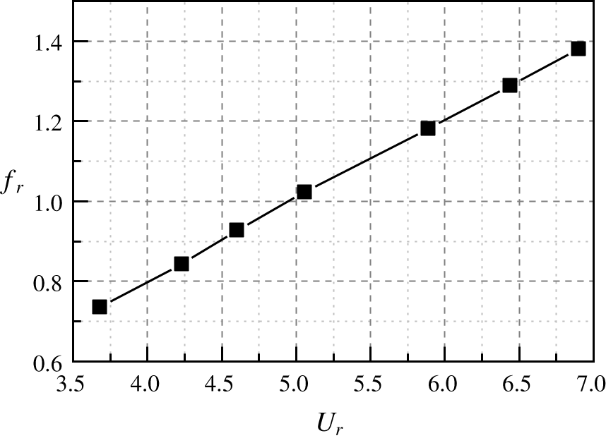
 $C_{L}$ is 0.57. In addition, the vortex shedding frequency increases linearly with the increasing flow velocity, as shown in figure 6. The predicted value of
 $St$ is in excellent agreement with the measurement of Mohany & Ziada (Reference Mohany and Ziada2011), both are 0.2. Moreover, the present prediction of
 $C_{L}$ is also in conformity with the published results for the flows in the same range of Reynolds number. For example, based on the experimental measurement by Norberg (Reference Norberg2003), the RMS value of
 $C_{L}$ is approximately 0.5, and the reported values of
 $C_{L}$ measured by Mohany & Ziada (Reference Mohany and Ziada2011) ranges from 0.23 to 0.89. The above results indicate that the main features and parameters of the vortex shedding from the cylinder have been reasonably depicted by DVM, which lays a solid foundation for the following sound field calculation.
Evolution of the vortex shedding behind a cylinder.

Vortex shedding results: (a) lift coefficient versus the non-dimensional time and (b) spectrum of lift coefficient.

Dependence of free vortex shedding frequency on flow velocity.

4.2 Sound field results
Both the flow and sound fields and their unsteady interaction are computed simultaneously in this section. Considering the time expense of the sound field solution, 33 800 steps are implemented in each case. The average time cost of each case is approximately 77 CPU hours. Among those steps, the last 32 768 steps corresponding to a physical time length of approximately 0.4 s are analysed using FFT. Accordingly, the frequency resolution is approximately 2.5 Hz, which is fine enough for localizing the resonant peaks in the spectra. As the 3-D correction method is operated in the frequency domain, only the sound pressure results relating to the frequency domain are corrected.
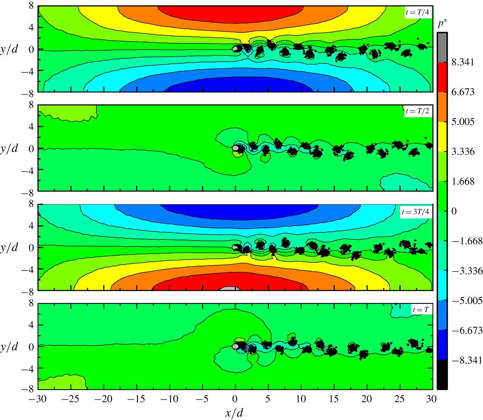
Figure 7 gives the sound field distribution within the duct at a reduced velocity of  $U_{r}=5.07$. The high-sound-pressure region appears regularly in the middle region of the duct where vortex shedding occurs. The sound pressure reaches positive and negative maxima on the duct wall just above and below the cylinder, respectively, and it decays rapidly in both the upstream and downstream directions. This is a typical sound pressure distribution pattern of the
 $\unicode[STIX]{x1D6FD}$-mode that relates to the first transverse acoustic mode of the duct (Mohany & Ziada Reference Mohany and Ziada2011). The present model gives the quantitative prediction of sound pressure distribution of the acoustic
 $\unicode[STIX]{x1D6FD}$-mode in the duct instead of qualitative results predicted by linear models.
Distribution of sound field at resonant state within a full cycle.

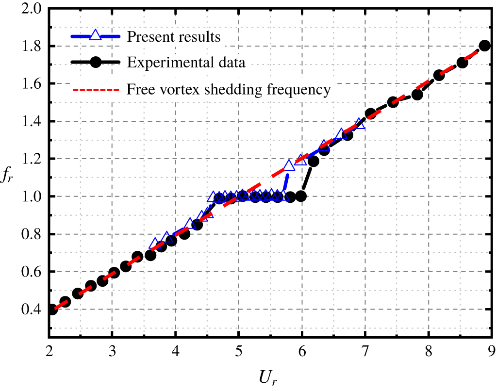
Dependence of resonant sound frequency on the flow velocity is shown in figure 8. When the reduced velocity,  $U_{r}$, increases from 3.69 to 4.61, the sound frequency stays identical with the vortex shedding frequency, which shows the same tendency with cases in free space (see figure 6). However, when the flow speed reaches
 $U_{r}=4.61$, where the vortex shedding of wake flow gets close to the inherent frequency of the acoustic
 $\unicode[STIX]{x1D6FD}$-mode of the duct, the vortex shedding frequency is shifted from its natural shedding frequency to be in conformity with the frequency of the
 $\unicode[STIX]{x1D6FD}$-mode. As the flow velocity increases slightly, the acoustical response of the
 $\unicode[STIX]{x1D6FD}$-mode is still strong enough to keep this mode up to the higher velocities, until it gets larger than
 $U_{r}=5.72$. In this respect, the lock-in regime is dominated by the acoustic
 $\unicode[STIX]{x1D6FD}$-mode. It is obvious that if the flow velocity further goes up, the vortex shedding will be locked onto higher-order acoustic modes. Although the higher-order lock-in phenomenon is not studied in the present work, it has been observed by previous experiment (Arafa & Mohany Reference Arafa and Mohany2019). It is the lock-in regime that characterizes the acoustic resonance. The predicted frequency of the
 $\unicode[STIX]{x1D6FD}$-mode,
 $f_{a}$, is determined by averaging the relevant frequencies of the peak values in the sound pressure spectrum during the lock-in region, which is approximately 686 Hz, in excellent agreement with the previous measured result of 688 Hz (Mohany & Ziada Reference Mohany and Ziada2011). From both the predicted results of
 $St$ and
 $f_{a}$, it confirms that the present 2-D model captures the features of both the flow and sound fields. To the authors’ knowledge, this is the first time that the lock-in phenomenon of acoustic resonance induced by the cylinder wake is captured with a nonlinear model. As shown in figure 8, the predicted frequency of sound pressure in the duct agrees well with the experimental data, except that the width of the lock-in region is under-predicted, where the predicted upper flow velocity is lower than the measured data by a discrepancy of
 $U_{r}=0.37$.
Dependence of resonant sound frequency on the increasing flow velocity.

Variation of resonant amplitude of sound pressure with the increasing flow velocity.

Waterfall plot of sound pressure spectra.

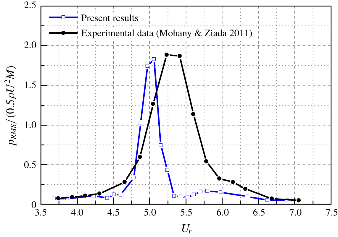
Figure 9 shows the variation of resonant amplitude of sound pressure with the increasing flow velocity, which is corrected with a 2-D to 3-D scaling law as given in (2.18). In general, a humped sound pressure curve is observed, and the peak value appears within the lock-in region corresponding to figure 8. With the reduced velocity increasing from 3.69 to 5.07, the non-dimensional sound pressure  $p^{\ast }$ goes up sharply from 0.08 to 1.88, then drastically falls back to 0.10 when the flow velocity reaches
 $U_{r}=5.54$. Being a 2-D sound model with a 3-D correction law, the predicted amplitude of sound pressure in the velocity range from 3.69 to 5.07 is in quite good agreement with the experimental data. Although the 3-D correction method has been usually used for the case of 2-D sound calculation in free space, the present comparison indicates that this method can also help to improve the accuracy of the sound pressure prediction within the 2-D flow duct.
As the reduced flow velocity further increases from 5.07 to 6.64, the deviation is seen between the predicted and measured sound pressure. The maximum sound pressure appears at the velocity of  $U_{r}=5.23$ in the experiment, whereas the predicted value is
 $U_{r}=5.07$. In this context, the velocity exciting the strongest resonance is under-predicted which is similar to the predicted lock-in region results in figure 8. Besides, it should be noted that the flow velocity corresponding to the maximum resonant sound pressure locates neither to where the free vortex shedding frequency is equal to the inherent
 $\unicode[STIX]{x1D6FD}$-mode frequency (
 $U_{r}\approx 4.98$), nor at the end of the lock-in region (
 $U_{r}=5.72$). This phenomenon has been detected in various experimental observations (Mohany & Ziada Reference Mohany and Ziada2009, Reference Mohany and Ziada2011; Arafa & Mohany Reference Arafa and Mohany2019), however, there is still a lack of a reasonable explanation to the relevance of the maximum sound pressure and the lock-in behaviour of vortex and resonant sound. Next, we will try to explore and understand the reasons behind the above phenomena, based on the present physical model.
4.3 Underlying mechanism of frequency lock-in phenomenon
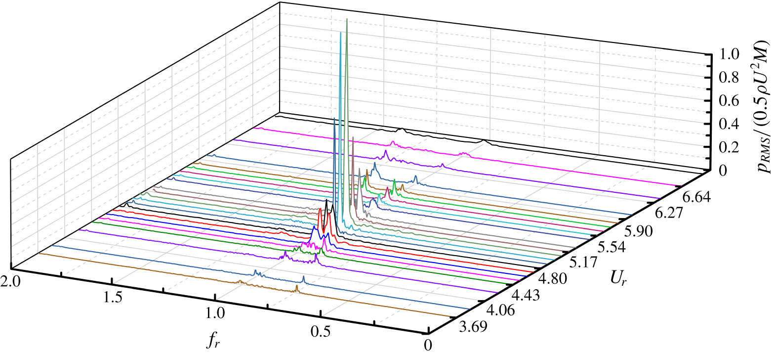
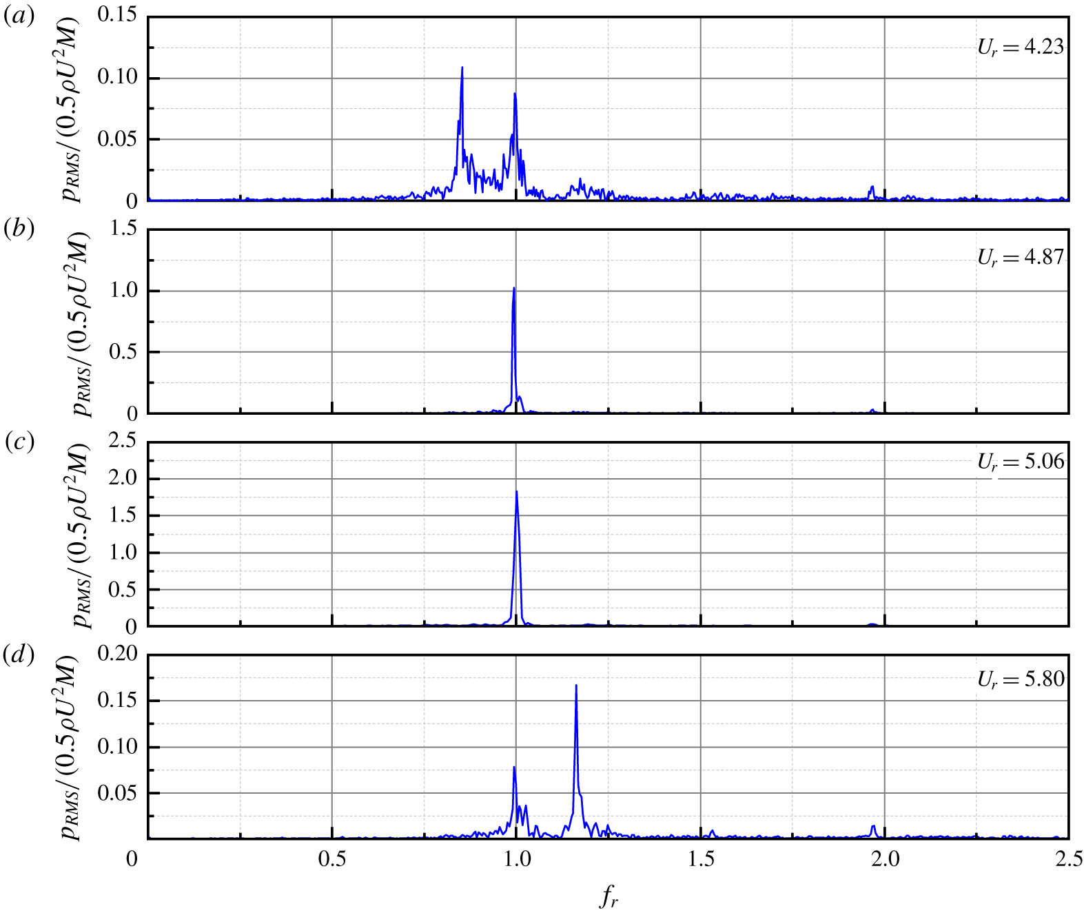
A waterfall plot of the sound pressure spectra monitored on the duct wall is given in figure 10, from which some typical frequency spectra are extracted, as shown in figure 11. Two dominant discrete frequency components co-exist in most cases: the one changing linearly with the incoming flow velocity is  $f_{s}$ and the other one remaining nearly constant around 686 Hz is
 $f_{a}$; this feature is in accordance with the previous experimental measurements (Mohany & Ziada Reference Mohany and Ziada2009, Reference Mohany and Ziada2011). A vigorous competition exists between these two frequencies. When the flow velocity is far from the lock-in region, the component corresponding to
 $f_{s}$ is higher than that of
 $f_{a}$. However, when the reduced velocity is in the range from 4.89 to 5.07, there is only one prominent tone component in the spectrum, which means the two frequencies are completely synchronized. In addition, the variations of
 $f_{s}$ and
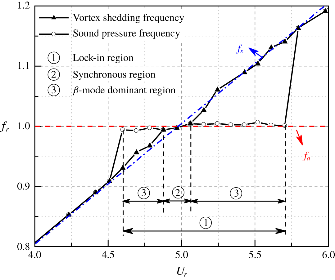
 $f_{a}$ with flow velocity are plotted in figure 11 for clarity. It is worth mentioning that, although the lock-in regime can be detected from 4.61 to 5.72, the synchronization of the vortex shedding and the sound wave can only be sustained in a narrow range between 4.89 and 5.07, out of which the vortex shedding frequency differs from the
 $\unicode[STIX]{x1D6FD}$-mode frequency. It is commonly accepted that during the lock-in region of acoustic resonance, the vortex shedding frequency is tuned to be in good agreement with the inherent frequency of resonant acoustic mode. However, this general description of lock-in phenomenon seems to overestimate the tuning effect of resonant sound. From the present results in figure 10, we can find that the vortex shedding frequency does not always stay the same as that of the resonant sound. But, the synchronization only exists in a relative narrower region, where the vortex shedding is fully locked to the resonant sound wave due to the feedback effect. Otherwise, most of the lock-in region beyond the synchronous region can be simply recognized as a forced response of the acoustic mode within the duct to the vortex shedding excitation.
Frequency spectra of sound pressure with typical flow velocities.

The flow duct can be recognized as a synchronous system with two oscillators: one is the vortex shedding from the cylinder (wake mode) and the other is the  $\unicode[STIX]{x1D6FD}$-mode sound wave within the duct (acoustic mode), and the acoustic particle velocity acts as the coupling between them. The forward part of this loop is the acoustic response of the duct excited by the fluctuating vortex shedding where
 $f_{s}$ and
 $f_{a}$ co-exist. When the mismatch between
 $f_{s}$ and
 $f_{a}$ is less than a threshold, the component corresponding to the
 $\unicode[STIX]{x1D6FD}$-mode would become dominant in the spectrum. The feedback part of this loop involves the tuning effect of the sound wave on the vortex shedding through acoustic particle velocity. When the two frequencies get close to each other, synchronization will occur, resulting in a single resonant frequency, as demonstrated in figure 12. In this aspect, it is reasonable to divide the lock-in region into two sub-regions: the synchronous region, where the frequencies of vortex shedding and sound wave combine into a common value (
 $0.98\leqslant f_{s}/f_{a}\leqslant 1.02$), and the
 $\unicode[STIX]{x1D6FD}$-mode dominant region where the component corresponding to
 $f_{a}$ is higher than that of
 $f_{s}$ (
 $0.93\leqslant f_{s}/f_{a}<0.98$,
 $1.02<f_{s}/f_{a}\leqslant 1.14$). There are two
 $\unicode[STIX]{x1D6FD}$-mode dominant regions on both sides of the synchronous region, and the right-hand one is slightly wider than the left-hand one, which is in conformity with the experimental observation of Mohany & Ziada (Reference Mohany and Ziada2011). These characteristics of lock-in regime in acoustic resonance are similar to those of the frequency lock-in for flow induced vibration (Zhang et al. Reference Zhang, Li, Ye and Jiang2015), where the lock-in regime is separated into ‘resonance-induced lock-in’ and ‘flutter-induced lock-in’ according to the frequency ratio between vortex shedding and structural vibration of the cylinder.
Frequencies of vortex shedding and sound in the duct with acoustic feedback.

Frequencies of vortex shedding and sound in the duct without acoustic feedback.

Frequencies of vortex shedding and sound pressure in free space.

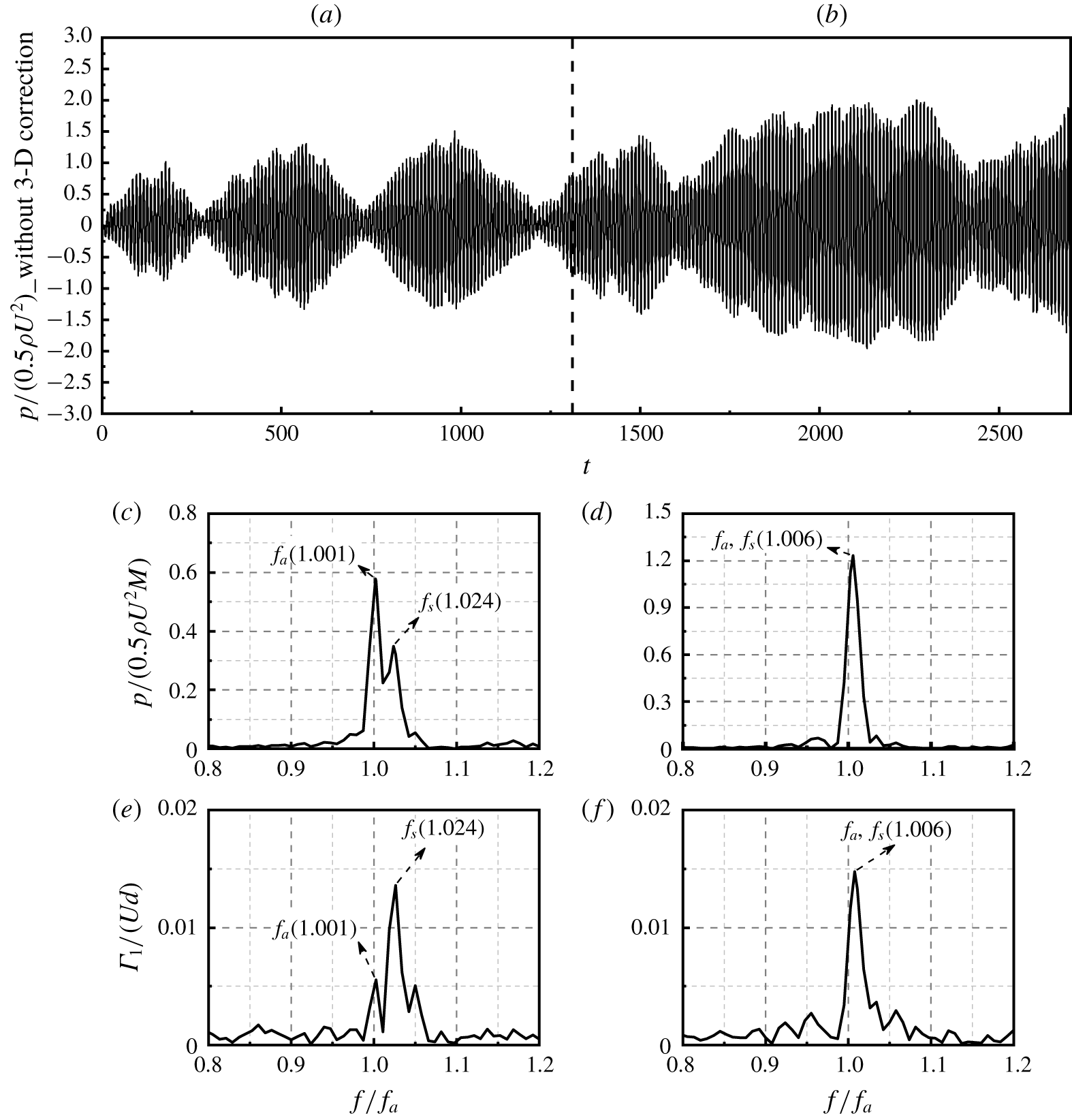
Time history of sound pressure and the corresponding spectra of sound pressure and vortex shedding for  $U_{r}=5.15$.

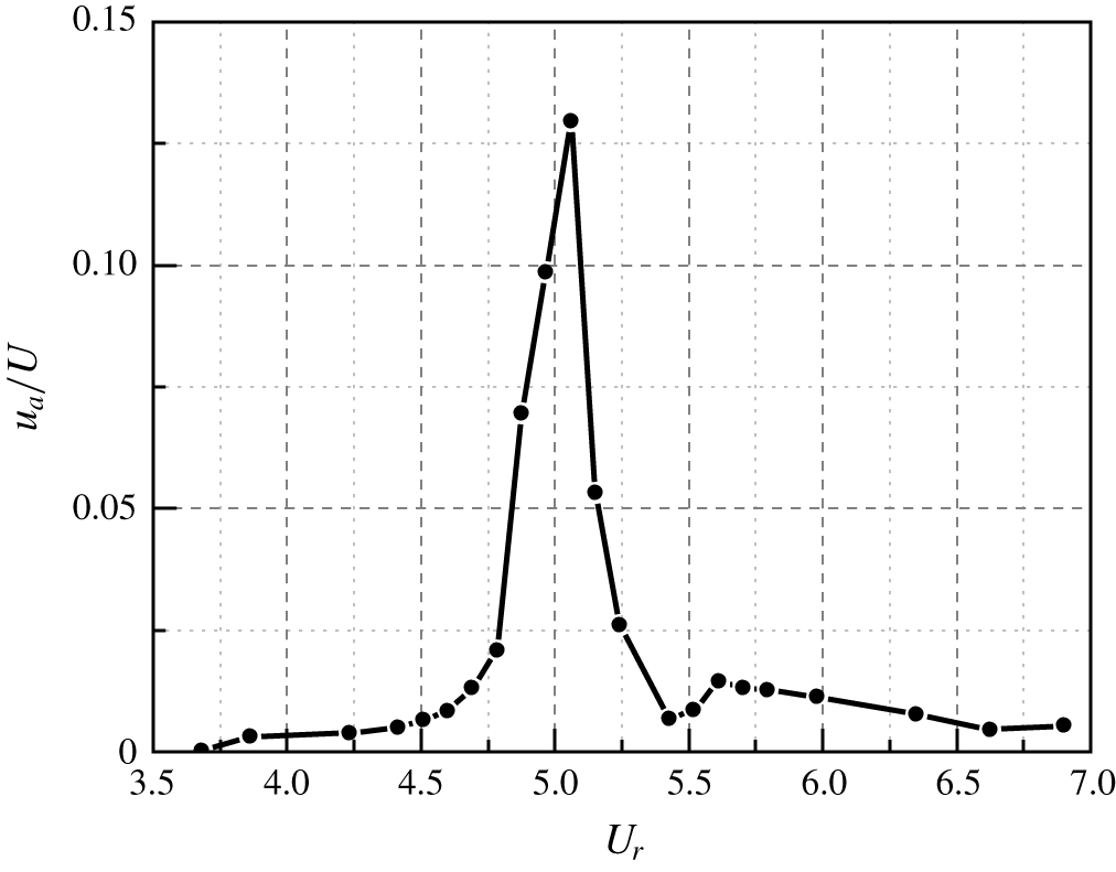
Velocity ratio of acoustic particle and incoming flow.

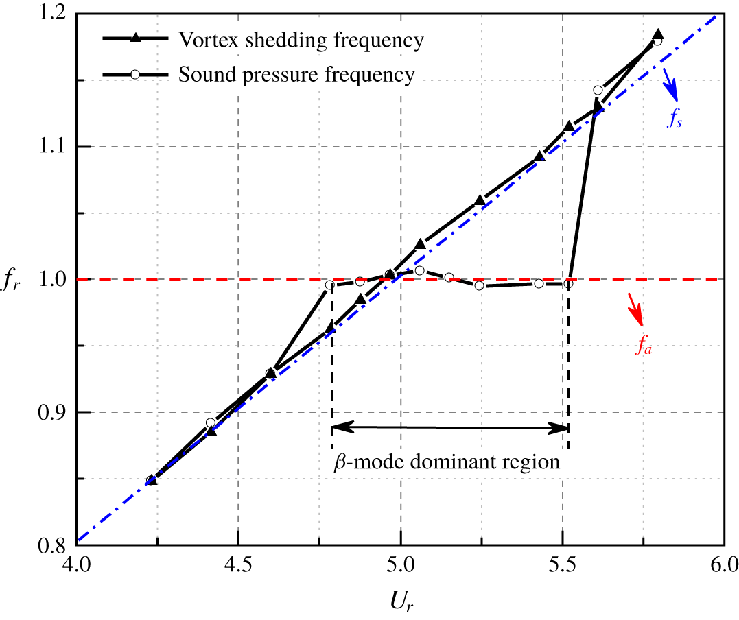
To evaluate the acoustic response of the present duct separately, the feedback from sound is removed, which can be readily realized by setting  $u_{a}=0$ in (2.16). Then, the dependence of the sound frequency results on the flow velocity is shown in figure 13. As can be seen, the general tendency is similar to the results shown in figure 8. Note that although the acoustic feedback is not involved in the computation, the
 $\unicode[STIX]{x1D6FD}$-mode dominant region within a narrower flow velocity range,
 $4.80\leqslant U_{r}\leqslant 5.63$, can also be found. In this context, the
 $\unicode[STIX]{x1D6FD}$-mode dominant region is actually the acoustic response of the duct excited by the vortex shedding, where the dominant component in sound spectra within the duct locks onto the inherent frequency of the
 $\unicode[STIX]{x1D6FD}$-mode. But the synchronous region totally disappears after the removal of feedback sound. The frequency of vortex shedding keeps to its natural shedding value, which indicates that the occurrence of synchronization is induced by the turning effect of the feedback sound.
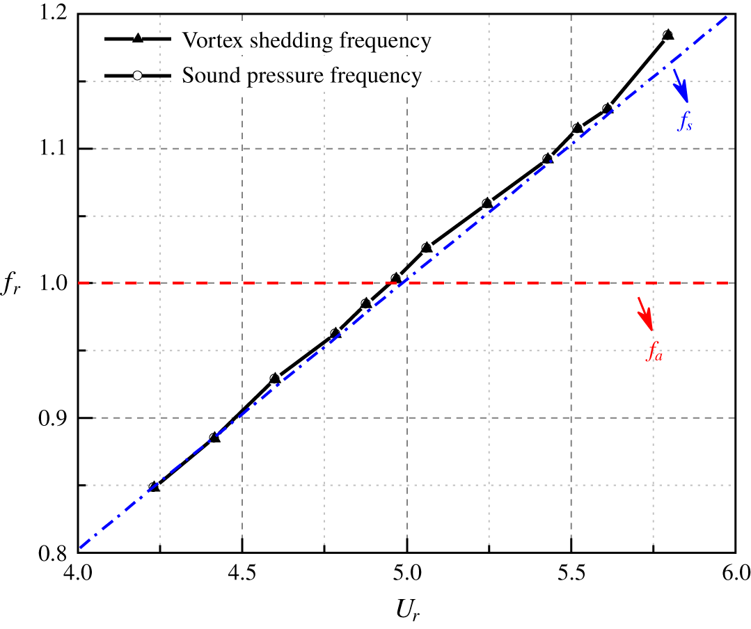
In order to illustrate the effect of the duct wall, the sound pressure results of vortex shedding behind the cylinder in free space are shown in figure 14. As is expected, the frequency of the sound wave is exactly in accordance with that of the vortex shedding for all the cases. Comparing the results shown in figures 12, 13 and 14, confirms that the lock-in phenomenon depends on the acoustic response of the duct, and the feedback effect is realized through the reflection of the sound wave by the duct walls.
From the view of the physical mechanism of acoustic resonance, it is expected that when the mismatch between  $f_{s}$ and
 $f_{a}$ is small enough, mutual capture would occur due to the feedback loop. Thus, it is interesting to explore the evolution behaviour of the mutual capturing. Figure 15 gives the time history and spectral information of the sound pressure and vortex shedding for
 $U_{r}=5.17$, where the spectra on the left and right-hand side in each row correspond to the front and rear half of the time history, respectively. As can be seen in figure 14(a), a rigorous competition between these
 $f_{s}$ and
 $f_{a}$ exists. At the beginning of the coupling process, a beat phenomenon happens and these two frequencies co-exist in the spectrum. While it is interesting that the dominant component is
 $f_{a}$ in the sound spectrum, it changes to
 $f_{s}$ in the flow field. This demonstrates that the duct acts as an amplifier to the sound wave in the whole synchronous system, which tends to enhance the component that nears the natural frequency of the
 $\unicode[STIX]{x1D6FD}$-mode. With the developing of the coupling process,
 $f_{a}$ gradually dominates the lock-in behaviour of the synchronous system, and causes
 $f_{s}$ to be fully synchronized to the natural frequency of the
 $\unicode[STIX]{x1D6FD}$-mode. These results show further evidence that the synchronous regime in acoustic resonance is caused by the feedback sound within the duct.
Another important aspect is that the strongest resonance appears at the end of synchronous region, which can be seen by comparing figures 9 and 12. In this aspect, the reasons for under-predicting the flow velocity corresponding to the strongest resonance and the upper bound of the lock-in region may be the same.
The reason may be due to the simplification of the boundary layer receptivity process in vortex shedding with acoustic feedback via directly adding acoustic particle velocity onto the potential flow. To improve the present model, a detailed instability analysis of the boundary layer together with the unsteady Kutta condition (Crighton Reference Crighton1985) at the separation point may be needed. Moreover, it is well known that apart from the frequency mismatch another parameter that affects the extent of the synchronization is the coupling strength, which is the acoustic particle velocity in this model. From figure 16 one can see that the ratio of the acoustic particle velocity to the incoming flow velocity is over 6 %, when the synchronization is sustained in the present simulation. Note that, if the coupling strength between the two oscillators is not sufficiently strong the synchronous regime may take a relative long time to set in (Pikovsky, Rosenblum & Kurths Reference Pikovsky, Rosenblum and Kurths2001). However, subjected to the computational cost of TDBEM in this time-domain physical model, the total length of the physical time is limited to approximately 0.4 s, which might be not long enough to fully develop the synchronization between the vortex shedding and the sound wave. As the coupling procedure developed, as shown in figure 15, the amplitude of sound pressure becomes larger and larger, which would promote the upper boundary of the lock-in region to higher velocities. In this aspect, this is another probably reason for the under-prediction of the width of lock-in region, which needs further improvement in the efficiency and stability for sound calculation.
5 Conclusions
An efficient nonlinear model is established to study the acoustic resonance induced by wake flow of a circular cylinder within a flow duct using meshless methods. It computes the flow field, sound field and their coupling simultaneously. The calculational domain is chosen to be in accordance with the previous experimental set-up. The typical characteristics of acoustic resonance are well captured and the underlying mechanism of frequency lock-in is deeply explored, although the quantitative precision of present model still has room for further improvement. The main conclusions are summarized as follows:
(1) The present model not only reasonably predicts the distribution of vortex street behind the cylinder and the sound pressure within the duct but also accurately gives the Strouhal number of the free vortex shedding and the inherent frequency of the
$\unicode[STIX]{x1D6FD}$-mode, which are validated by previous experimental data.(2) The characteristics of the lock-in phenomenon in flow-induced acoustic resonance are reasonably captured by the present model. The tendency of frequency and amplitude of resonant sound with the increasing flow velocity agree well with the experimental data, but the extent of lock-in region is under-predicted.
(3) The flow duct containing a cylinder can be recognized as a synchronous system with two oscillators: the vortex shedding (wake mode) and the
$\unicode[STIX]{x1D6FD}$-mode (acoustic mode). The underlying mechanism of lock-in is represented as the vigorous competition between these two oscillators, and the extent of the lock-in region is dominated by the acoustic mode.(4) Two kinds of lock-in regions, the synchronous region and the
$\unicode[STIX]{x1D6FD}$-mode dominant region, are identified depending on the frequency mismatch between $f_{s}$ and $f_{a}$. The synchronous region is found when the $f_{s}$ approaches $f_{a}$ ($0.98\leqslant f_{s}/f_{a}\leqslant 1.02$) and the corresponding velocity ratio of the acoustic particle velocity to the incoming flow is over 6 %. Meanwhile, the $\unicode[STIX]{x1D6FD}$-mode dominant region is detected when the frequency mismatch is slightly larger ($0.93\leqslant f_{s}/f_{a}<0.98$ and $1.02<f_{s}/f_{a}\leqslant 1.14$). The $\unicode[STIX]{x1D6FD}$-mode dominant region is dominated by the acoustic response of the duct to the vortex shedding excitation, while the synchronous region is produced by the tuning effect of the feedback sound.(5) The maximum sound pressure appears at the end of the synchronous region, which locates at a higher velocity than that where
$f_{s}$ exactly equals $f_{a}$, this is the most distinct feature of the present synchronous system that differs from the forced excitation systems.








Acknowledgements
The authors gratefully acknowledge the financial support from National Natural Science Foundation of China (51806146, 51790514, 51676008, 51576009, U1633113).
Declaration of interests
The authors report no conflict of interest.
Appendix A. Derivation of sound pressure radiated from a point vortex
According to (2.9) in § 2, the general solution of the sound pressure radiated from the  $n$th point vortex that locates at
 $\boldsymbol{s}(y_{1n},y_{2n})$ is expressed as
 $$\begin{eqnarray}\frac{p_{n}}{\unicode[STIX]{x1D70C}_{0}}=-\int _{0}^{t}\int _{\unicode[STIX]{x1D6FA}}(\unicode[STIX]{x1D74E}_{n}\times \boldsymbol{v}_{n})\boldsymbol{\cdot }\unicode[STIX]{x1D735}G\,\text{d}\unicode[STIX]{x1D6FA}\,\text{d}\unicode[STIX]{x1D70F},\end{eqnarray}$$
where  $\unicode[STIX]{x1D74E}_{n}$ and
 $\boldsymbol{v}_{n}$ are the vorticity and the convection velocity of the
 $n$th point vortex,
 $\unicode[STIX]{x1D74E}_{n}=\boldsymbol{k}\unicode[STIX]{x1D6E4}_{n}\unicode[STIX]{x1D6FF}(y_{1}-y_{1n}(\unicode[STIX]{x1D70F}))(y_{2}-y_{2n}(\unicode[STIX]{x1D70F}))$,
 $\boldsymbol{v}_{n}=\boldsymbol{i}u_{n}+\boldsymbol{j}v_{n}$ and
 $\boldsymbol{i}$,
 $\boldsymbol{j}$,
 $\boldsymbol{k}$ refer to the unit vectors directed along the three positive axes.
Substituting the expressions of  $\unicode[STIX]{x1D74E}_{n}$ and
 $\boldsymbol{v}_{n}$ in to (A 1), we have
 $$\begin{eqnarray}\displaystyle \frac{p_{n}}{\unicode[STIX]{x1D70C}_{0}} & = & \displaystyle -\int _{0}^{t}\int _{\unicode[STIX]{x1D6FA}} [\boldsymbol{j}\unicode[STIX]{x1D6E4}_{n}u_{n}\unicode[STIX]{x1D6FF}(y_{1}-y_{1n}(\unicode[STIX]{x1D70F}))(y_{2}-y_{2n}(\unicode[STIX]{x1D70F}))\nonumber\\ \displaystyle & & \displaystyle -\,\boldsymbol{i}\unicode[STIX]{x1D6E4}_{n}v_{n}\unicode[STIX]{x1D6FF}(y_{1}-y_{1n}(\unicode[STIX]{x1D70F}))(y_{2}-y_{2n}(\unicode[STIX]{x1D70F}))\!]\boldsymbol{\cdot }\left(\boldsymbol{i}\frac{\unicode[STIX]{x2202}G}{\unicode[STIX]{x2202}y_{1}}+\boldsymbol{j}\frac{\unicode[STIX]{x2202}G}{\unicode[STIX]{x2202}y_{2}}\right)\,\text{d}y_{1}y_{2}\,\text{d}\unicode[STIX]{x1D70F}\nonumber\\ \displaystyle & = & \displaystyle \left.\int _{0}^{t}\unicode[STIX]{x1D6E4}_{n}v_{n}\frac{\unicode[STIX]{x2202}G}{\unicode[STIX]{x2202}y_{1}}\right|_{(y_{1n}(\unicode[STIX]{x1D70F}),y_{2n}(\unicode[STIX]{x1D70F}),\unicode[STIX]{x1D70F})}\,\text{d}\unicode[STIX]{x1D70F}-\left.\int _{0}^{t}\unicode[STIX]{x1D6E4}_{n}u_{n}\frac{\unicode[STIX]{x2202}G}{\unicode[STIX]{x2202}y_{2}}\right|_{(y_{1n}(\unicode[STIX]{x1D70F}),y_{2n}(\unicode[STIX]{x1D70F}),\unicode[STIX]{x1D70F})}\,\text{d}\unicode[STIX]{x1D70F}.\end{eqnarray}$$
Substitute the 2-D free space Green’s function, (2.10), into (A 2), and the first integral term on the right-hand side would be first deduced. The partial derivative term in the  $y_{1}$ direction yields
 $$\begin{eqnarray}\frac{\unicode[STIX]{x2202}G}{\unicode[STIX]{x2202}y_{1}}=\frac{\unicode[STIX]{x2202}R}{\unicode[STIX]{x2202}y_{1}}\frac{c_{0}RH[c_{0}(t-\unicode[STIX]{x1D70F})-R]}{2\unicode[STIX]{x03C0}\sqrt{[c_{0}^{2}(t-\unicode[STIX]{x1D70F})^{2}-R^{2}]^{3}}}+\frac{\unicode[STIX]{x2202}R}{\unicode[STIX]{x2202}y_{1}}\frac{c_{0}\frac{\unicode[STIX]{x2202}}{\unicode[STIX]{x2202}R}(H[c_{0}(t-\unicode[STIX]{x1D70F})-R])}{2\unicode[STIX]{x03C0}\sqrt{c_{0}^{2}(t-\unicode[STIX]{x1D70F})^{2}-R^{2}}},\end{eqnarray}$$
where  $R$ is the distance between the observation point and the source point. Further operations are needed using the following relation
 $$\begin{eqnarray}\frac{\unicode[STIX]{x2202}}{\unicode[STIX]{x2202}R}(H[c_{0}(t-\unicode[STIX]{x1D70F})-R])=\frac{1}{c_{0}}\frac{\unicode[STIX]{x2202}}{\unicode[STIX]{x2202}\unicode[STIX]{x1D70F}}H[R-c_{0}(t-\unicode[STIX]{x1D70F})].\end{eqnarray}$$
After that, the first term on the right-hand side of (A 2) is written as
 $$\begin{eqnarray}\displaystyle \int _{0}^{t}\left.\unicode[STIX]{x1D6E4}_{n}v_{n}\frac{\unicode[STIX]{x2202}G}{\unicode[STIX]{x2202}y_{1}}\right|_{(y_{1n}(\unicode[STIX]{x1D70F}),y_{2n}(\unicode[STIX]{x1D70F}),\unicode[STIX]{x1D70F})}\,\text{d}\unicode[STIX]{x1D70F} & = & \displaystyle \int _{0}^{t}\unicode[STIX]{x1D6E4}_{n}v_{n}\frac{\unicode[STIX]{x2202}R}{\unicode[STIX]{x2202}y_{1}}\frac{c_{0}RH[c_{0}(t-\unicode[STIX]{x1D70F})-R]}{2\unicode[STIX]{x03C0}\sqrt{[c_{0}^{2}(t-\unicode[STIX]{x1D70F})^{2}-R^{2}]^{3}}}\,\text{d}\unicode[STIX]{x1D70F}\nonumber\\ \displaystyle & & \displaystyle +\,\int _{0}^{t}\unicode[STIX]{x1D6E4}_{n}v_{n}\frac{\unicode[STIX]{x2202}R}{\unicode[STIX]{x2202}y_{1}}\frac{\displaystyle \frac{\unicode[STIX]{x2202}}{\unicode[STIX]{x2202}\unicode[STIX]{x1D70F}}H[R-c_{0}(t-\unicode[STIX]{x1D70F})]}{2\unicode[STIX]{x03C0}\sqrt{c_{0}^{2}(t-\unicode[STIX]{x1D70F})^{2}-R^{2}}}\,\text{d}\unicode[STIX]{x1D70F}.\end{eqnarray}$$
The second integral term of (A 5),  $I_{2}$, can be integrated by parts with respect to
 $\unicode[STIX]{x1D70F}$, which is given as
 $$\begin{eqnarray}\displaystyle I_{2} & = & \displaystyle -\int _{0}^{t}\frac{\displaystyle \unicode[STIX]{x2202}\left(\unicode[STIX]{x1D6E4}_{n}v_{n}\frac{\unicode[STIX]{x2202}R}{\unicode[STIX]{x2202}y_{1}}\right)}{\unicode[STIX]{x2202}\unicode[STIX]{x1D70F}}\frac{H[c_{0}(t-\unicode[STIX]{x1D70F})-R]}{2\unicode[STIX]{x03C0}\sqrt{c_{0}^{2}(t-\unicode[STIX]{x1D70F})^{2}-R^{2}}}\,\text{d}\unicode[STIX]{x1D70F}\nonumber\\ \displaystyle & & \displaystyle -\,\int _{0}^{t}\unicode[STIX]{x1D6E4}_{n}v_{n}\frac{\unicode[STIX]{x2202}R}{\unicode[STIX]{x2202}y_{1}}\frac{\displaystyle c_{0}^{2}(t-\unicode[STIX]{x1D70F})+R\frac{\unicode[STIX]{x2202}R}{\unicode[STIX]{x2202}\unicode[STIX]{x1D70F}}}{2\unicode[STIX]{x03C0}(\sqrt{c_{0}^{2}(t-\unicode[STIX]{x1D70F})^{2}-R^{2}})^{3}}H[c_{0}(t-\unicode[STIX]{x1D70F})-R]\,\text{d}\unicode[STIX]{x1D70F}.\end{eqnarray}$$
In a low Mach number flow, the convection effect of the flow field on the sound wave propagation can be neglected, then we have
 $$\begin{eqnarray}\displaystyle I_{2} & {\approx} & \displaystyle -\int _{0}^{t}\frac{\displaystyle \unicode[STIX]{x2202}\left(\unicode[STIX]{x1D6E4}_{n}v_{n}\frac{\unicode[STIX]{x2202}R}{\unicode[STIX]{x2202}y_{1}}\right)}{\unicode[STIX]{x2202}\unicode[STIX]{x1D70F}}\frac{H[c_{0}(t-\unicode[STIX]{x1D70F})-R]}{2\unicode[STIX]{x03C0}\sqrt{c_{0}^{2}(t-\unicode[STIX]{x1D70F})^{2}-R^{2}}}\,\text{d}\unicode[STIX]{x1D70F}\nonumber\\ \displaystyle & & \displaystyle -\,\int _{0}^{t}\unicode[STIX]{x1D6E4}_{n}v_{n}\frac{\unicode[STIX]{x2202}R}{\unicode[STIX]{x2202}y_{1}}\frac{c_{0}^{2}(t-\unicode[STIX]{x1D70F})H[c_{0}(t-\unicode[STIX]{x1D70F})-R]}{2\unicode[STIX]{x03C0}(\sqrt{c_{0}^{2}(t-\unicode[STIX]{x1D70F})^{2}-R^{2}})^{3}}\,\text{d}\unicode[STIX]{x1D70F}.\end{eqnarray}$$
Thus, the first term on the right-hand side of (A 2) is finally expressed as
 $$\begin{eqnarray}\displaystyle & & \displaystyle \int _{0}^{t}\left.\unicode[STIX]{x1D6E4}_{n}v_{n}\frac{\unicode[STIX]{x2202}G}{\unicode[STIX]{x2202}y_{1}}\right|_{(y_{1n}(\unicode[STIX]{x1D70F}),y_{2n}(\unicode[STIX]{x1D70F}),\unicode[STIX]{x1D70F})}\,\text{d}\unicode[STIX]{x1D70F}\nonumber\\ \displaystyle & & \displaystyle \quad =-\int _{0}^{t}\left(\unicode[STIX]{x1D6E4}_{n}v_{n}\frac{\unicode[STIX]{x2202}R}{\unicode[STIX]{x2202}y_{1}}\right)\frac{c_{0}[c_{0}(t-\unicode[STIX]{x1D70F})-R]H[c_{0}(t-\unicode[STIX]{x1D70F})-R]}{2\unicode[STIX]{x03C0}(\sqrt{c_{0}^{2}(t-\unicode[STIX]{x1D70F})^{2}-R^{2}})^{3}}\,\text{d}\unicode[STIX]{x1D70F}\nonumber\\ \displaystyle & & \displaystyle \qquad -\,\int _{0}^{t}\frac{\displaystyle \unicode[STIX]{x2202}\left(\unicode[STIX]{x1D6E4}_{n}v_{n}\frac{\unicode[STIX]{x2202}R}{\unicode[STIX]{x2202}y_{1}}\right)}{\unicode[STIX]{x2202}\unicode[STIX]{x1D70F}}\frac{H[c_{0}(t-\unicode[STIX]{x1D70F})-R]}{2\unicode[STIX]{x03C0}\sqrt{c_{0}^{2}(t-\unicode[STIX]{x1D70F})^{2}-R^{2}}}\,\text{d}\unicode[STIX]{x1D70F}.\end{eqnarray}$$
Similarly, the second term on the right-hand side of (A 2) is readily written as
 $$\begin{eqnarray}\displaystyle & & \displaystyle -\int _{0}^{t}\left.\unicode[STIX]{x1D6E4}_{n}u_{n}\frac{\unicode[STIX]{x2202}G}{\unicode[STIX]{x2202}y_{2}}\right|_{(y_{1n}(\unicode[STIX]{x1D70F}),y_{2n}(\unicode[STIX]{x1D70F}),\unicode[STIX]{x1D70F})}\,\text{d}\unicode[STIX]{x1D70F}\nonumber\\ \displaystyle & & \displaystyle \quad =\int _{0}^{t}\left(\unicode[STIX]{x1D6E4}_{n}u_{n}\frac{\unicode[STIX]{x2202}R}{\unicode[STIX]{x2202}y_{2}}\right)\frac{c_{0}[c_{0}(t-\unicode[STIX]{x1D70F})-R]H[c_{0}(t-\unicode[STIX]{x1D70F})-R]}{2\unicode[STIX]{x03C0}(\sqrt{c_{0}^{2}(t-\unicode[STIX]{x1D70F})^{2}-R^{2}})^{3}}\,\text{d}\unicode[STIX]{x1D70F}\nonumber\\ \displaystyle & & \displaystyle \qquad +\,\int _{0}^{t}\frac{\displaystyle \unicode[STIX]{x2202}\left(\unicode[STIX]{x1D6E4}_{n}u_{n}\frac{\unicode[STIX]{x2202}R}{\unicode[STIX]{x2202}y_{2}}\right)}{\unicode[STIX]{x2202}\unicode[STIX]{x1D70F}}\frac{H[c_{0}(t-\unicode[STIX]{x1D70F})-R]}{2\unicode[STIX]{x03C0}\sqrt{c_{0}^{2}(t-\unicode[STIX]{x1D70F})^{2}-R^{2}}}\,\text{d}\unicode[STIX]{x1D70F}.\end{eqnarray}$$
Substituting (A 8), (A 9) into (A 2), the sound pressure radiated from the  $n$th vortex can be finally given as
 $$\begin{eqnarray}\displaystyle \frac{p_{n}}{\unicode[STIX]{x1D70C}_{0}} & = & \displaystyle \int _{0}^{t}\unicode[STIX]{x1D6E4}_{n}\left(u_{n}\frac{\unicode[STIX]{x2202}R}{\unicode[STIX]{x2202}y_{2}}-v_{n}\frac{\unicode[STIX]{x2202}R}{\unicode[STIX]{x2202}y_{1}}\right)\frac{c_{0}[c_{0}(t-\unicode[STIX]{x1D70F})-R]H[c_{0}(t-\unicode[STIX]{x1D70F})-R]}{2\unicode[STIX]{x03C0}\sqrt{[c_{0}^{2}(t-\unicode[STIX]{x1D70F})^{2}-R^{2}]^{3}}}\,\text{d}\unicode[STIX]{x1D70F}\nonumber\\ \displaystyle & & \displaystyle +\,\int _{0}^{t}\frac{\displaystyle \unicode[STIX]{x2202}\left[\unicode[STIX]{x1D6E4}_{n}\left(u_{n}\frac{\unicode[STIX]{x2202}R}{\unicode[STIX]{x2202}y_{2}}-v_{n}\frac{\unicode[STIX]{x2202}R}{\unicode[STIX]{x2202}y_{1}}\right)\right]}{\unicode[STIX]{x2202}\unicode[STIX]{x1D70F}}\frac{H[c_{0}(t-\unicode[STIX]{x1D70F})-R]}{2\unicode[STIX]{x03C0}\sqrt{c_{0}^{2}(t-\unicode[STIX]{x1D70F})^{2}-R^{2}}}\,\text{d}\unicode[STIX]{x1D70F}.\end{eqnarray}$$