1. INTRODUCTION
In air transportation, proper handling of conflicts is critical so as to avoid accidents and incidents. For air traffic management, Air Traffic Controllers (ATCOs) are responsible for the safe command and control of aircraft through an airspace under the charge of the Air Traffic Control (ATC) service (International Civil Aviation Organization (ICAO), 1994). To do so, ATCOs need to monitor the aircraft on a radar screen and guide the aircraft safely through the airspace by issuing correct instructions with minimal margin of error in terms of accidents and incidents while adhering to very high safety standards.
In recent years, Air Traffic Management (ATM) has been undergoing dynamic and major changes, with two major programmes being initiated in the Single European Sky ATM Research Programme (SESAR) by Eurocontrol and the NextGen programme by the Federal Aviation Administration (FAA). A key goal of these programmes is to develop future technologies that will facilitate traffic growth forecast at an annual 4% rate of increase to 2020 (ICAO, 2014). At the same time, improvements to traffic safety within the airspace and air transport system need to be made. One emerging technological approach concerns the adoption of Four-Dimensional Trajectory Based Operations (4D-TBO), where the flight trajectory of aircraft can be predicted in a more timely, accurate and consistent manner. As a result, aircraft will be freer to fly on their own desired trajectories, creating a more complex air route structure with tighter separation standards (Enea and Porretta, Reference Enea and Porretta2012; Bowen, Reference Bowen2014; Mutuel et al., Reference Mutuel, Neri and Paricaud2013). This in turn will increase the complexity of future airspace and traffic flow patterns. Based on present practice, this would invariably impact on the ATCO's operational performance and taskload in terms of tactical radar monitoring, guiding of aircraft movements and maintaining high operational safety standards. To better aid ATCOs in their monitoring performance as well as taskload planning and management, air traffic complexity measurement approaches have been suggested in which regions of varying levels of complexity can be evaluated.
2. A REVIEW OF AIR TRAFFIC COMPLEXITY APPROACHES
Air traffic complexity represents a significant portion of an ATC workload. Its complexity is multi-dimensional and is dependent on static sector characteristics and dynamic traffic patterns (Mogford et al., Reference Mogford, Guttman, Morrow and Kopardekar1995). It is defined as “how difficult a given traffic situation is, based on the control activity required to resolve it and respond to an additional aircraft entering the airspace” (Lee et al., Reference Lee, Feron and Pritchett2007). To determine the level of air traffic complexity of a given sector, a review into several commonly used methods to validate air traffic complexity will be discussed in this paper.
A very well-known complexity metric approach is Dynamic Density (DD) developed by Laudeman et al. (Reference Laudeman, Shelden, Branstrom and Brasil1998) at the National Aeronautical and Space Agency (NASA). The DD approach consisted of eight traffic complexity terms such as number of heading changes, number of speed changes, number of altitude changes, number of aircraft with a Three-Dimensional (3D) Euclidean distance of 0 to 5 and 0 to 25 nautical miles and the number of conflicts predicted in 0–25, 25–40 and 40–70 nautical miles. Others like Kopardekar and Magyarits (Reference Kopardekar and Magyarits2002; Reference Kopardekar and Magyarits2003), Kopardekar et al. (Reference Kopardekar, Schwartz, Magyarits and Rhodes2009), Sridhar et al. (Reference Sridhar, Sheth and Grabbe1998) and Masalonis et al. (Reference Masalonis, Callaham and Wanke2003) have refined the approach to include proximity measurements, conflict state and time horizon, while Masalonis et al. (Reference Masalonis, Callaham and Wanke2003) have also included aircraft's intent and only used metrics that represent an aircraft's characteristics. These approaches aimed to better help strategic planners to make better traffic flow management decisions while minimising airspace overload. Nevertheless, such complexity models do not account for individual flight orientation and location. Although DD and its variants can provide some degree of robust evaluation of the airspace complexity at hand, these approaches rely mainly on historical rather than real-time data. Derivation of complexity levels for tactical use would therefore not be appropriate. Besides, for tactical radar control, ATCOs would need to look at the radar display and display information with reference to the orientation and locations to the origin to perform their tasks. Such information is not captured via these approaches.
Another commonly used model by Chatterji and Sridhar (Reference Chatterji and Sridhar2001) seeks to measure air traffic complexity using a set of 16 terms, which are descriptors of traffic pattern based on its second order statistical measures of the positions and velocities of the aircraft. These measures include traffic volume, aircraft separation between pairs, distribution of aircraft pattern, speed and mix, closing rate of one aircraft with respect to another aircraft and conflict level of resolution. Temporal proximity conflict calculation between aircraft was performed pairwise by taking into consideration the vertical and lateral separations. This complexity metric seeks to use a precise pairwise calculation to determine the conflict characteristics of an aircraft, discounting manoeuvres with no effect on complexity. This model is, however, limited to individual evaluation of an aircraft pair and does not capture the aircraft's intent among various aircraft operating within that region.
In the approach of Boag et al. (Reference Boag, Neal, Loft and Halford2006), relative terms between aircraft parameters were used to compute its relational complexity. Variables such as relative flight level, relative speed and relative trajectory are used to compute the relational complexity. Their complexity metric focused on the temporal sequence of separation standards, by assigning a relational complexity value to the time that the aircraft pairs lose separation. Four variables relating to the time when the aircraft pairing enters and leaves conflict, lateral and vertical conflict types were used to determine five levels of relational complexity. Such a complexity computation is purely based on the timing that an aircraft pairing enters and leaves the conflict. In Radanovic et al. (Reference Radanovic, Eroles, Koca and Nieto2017), a concurrence events identification complexity model was used to identify and assess impending conflict situations. This model used the projection of an aircraft's 4D trajectory to compute the traffic complexity in a tactical situation. An intent-based conflict detection algorithm was first applied to determine the conflict probability from the 4D trajectory of aircraft pairings at the 3D point in a designated airspace. A cluster of aircraft can be evaluated by extending the envelope boundary with respect to the 3D point. Complexity was computed using the aircraft count and evolving 4D geometries within this extended cluster. These models suffer from prediction inaccuracy when impending conflicts have been resolved beforehand, as complexities are only computed in conflict scenarios. It is therefore clear that neither relational nor concurrence events identification models are able to evaluate varying traffic patterns and situations.
In Delahaye and Puechmorel (Reference Delahaye and Puechmorel2000) and Puechmorel and Delahaye (Reference Puechmorel and Delahaye2009) dynamic system theory coupled with Kolmogorov-Entropy (Kolmogorov, Reference Kolmogorov1959) was used to compute traffic complexity. This was done by quantifying the level of disorder in the aircraft's trajectory within a designated airspace. Relative displacement and velocities between aircraft pairs were used to compute a density function, a convergence and divergence function together with a sensitivity function. Kolmogorov-Entropy was then used to calculate the intrinsic complexity for a designated airspace topology. A final complexity indicator, deduced from four derived functions, seeks to provide the situation complexity by taking into account the aircraft's current position and velocity, as well as a broad spectrum of traffic patterns and situations. The approach used instantaneous values of aircraft characteristics thereby making it suitable for computing tactical traffic complexity. However, it was not able to pinpoint exactly where the key conflict lies, as the final complexity score is of a higher order term derived from the sum of relative displacement and velocities of all aircraft pairs.
2.1. Evaluation of present air traffic complexity approaches
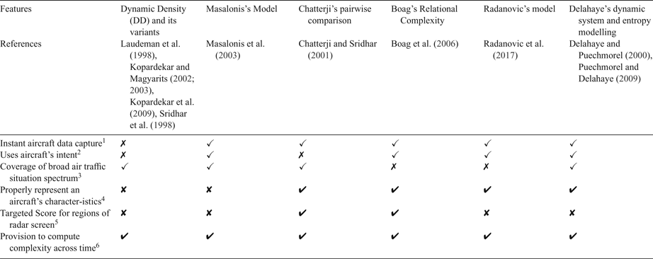
In order to establish a suitable complexity indicator to compute tactical complexity to aid ATCOs in the operation of their tasks, the approach should have the following desirable features. This includes the ability to perform instantaneous aircraft data capture for real-time computation to facilitate tactical monitoring, projection of an aircraft's flight intent (Endsley and Garland, Reference Endsley and Garland2000; Endsley, Reference Endsley2011; Masalonis et al., Reference Masalonis, Callaham and Wanke2003), capability to evaluate a broad spectrum of air traffic situations, dynamic and meaningful representation of changes to aircraft characteristics (Masalonis et al., Reference Masalonis, Callaham and Wanke2003), determination of various complexity scores at different regions on the radar screen to enhance tactical monitoring performance (Kang and Landry, Reference Kang and Landry2015; Wee et al., Reference Wee, Lye and Pinheiro2017a) and to compute complexity change across time. Table 1 compares the various reviewed approaches against a set of six desirable features used to determine traffic complexity. From Table 1, Chatterji's pairwise comparison, Boag's Relational Complexity and Delahaye's dynamic system and entropy modelling best satisfy the set of desired features for the traffic complexity model, with DD and its variants satisfying the least.
Feature comparison of existing complexity indicators adopted.

1 Instantaneous aircraft data capture is necessary for real time computation of complexity for tactical ATC.
2 Aircraft's intent is required as ATCOs project them for their tactical monitoring tasks.
3 Coverage of the broad air traffic situation is necessary as it is dynamic and varies across time.
4 Proper representation of an aircraft's characteristics is necessary so that any complexity computation is reflective of air traffic complexity in tactical monitoring. This includes an individual flight's space and time information, location and orientation with respect to the radar screen, while discounting irrelevant parameters.
5 A targeted, detailed complexity is required on different regions of the radar screen, as ATCOs tend to monitor the radar screen in different regions and zones.
6 Complexity should be able to be computed across time, in order to study the changes in complexity level of tactical ATC at different time instances.
3. PROPOSED CONFLICT ACTIVITY LEVEL COMPLEXITY MODEL
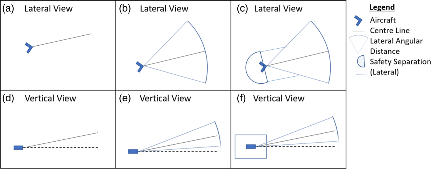
This section proposes a tactical complexity approach that makes use of all the six desired features where instantaneous aircraft data are captured together with its intent, covering a broad spectrum of air traffic situations with meaningful representation of aircraft characteristics, while determining the spatial complexity in real time (both instantaneous and duration of time) of any designated region(s) on the radar screen. The approach makes use of data obtained from current and projected aircraft's position and trajectory, which involves three main steps. These are the establishment of the flight conflict shape movement, traffic complexity Conflict Activity Level (CAL) and overall complexity score of the region. Derivation of the flight conflict shape movement is illustrated in Figure 1.
(a–f) Establishment of an aircraft's conflict shape movement.

3.1. Flight conflict shape movement
The flight conflict shape movement represents the extent to which the aircraft would be in opposition with other traffic or exogenous factors such as weather and emergency situation. In this work, the tactical conflict shape movement of an aircraft flying in an airspace is established based on its current position and trajectory, its likely angle of deviation from its current trajectory and the safety standards imposed in the airspace in which it is flying.
Figure 1 shows the lateral and vertical views of the derived flight conflict shape movement. In the lateral view, the conflict shape movement consists of the front and back portions. The front portion highlights the forward movement of the aircraft designated by an arrow symbol which denotes its current position and trajectory (centreline). The length and direction of the centreline corresponds to the speed and heading of the aircraft, respectively. As the aircraft may deviate from its trajectory, this is accounted for by a drift angle, θ to the left and right of the centreline giving rise to an arc sector (ICAO, 2009). To meet the Required Navigational Performance (RNP) standard of the airspace, a rectangular block is used to form the lateral region around the airspace at the front portion of the aircraft. Any deviation of lateral aircraft movement is accounted for in this rectangular block whenever RNP standards are larger than radar surveillance lateral separation distance between aircraft. On the back portion of the aircraft, this is represented by a semi-circle, taking into account the wake turbulence separation standard.
In the vertical view, the rate of climb/descent of the aircraft is determined based on the aircraft vertical trajectory and the corresponding vertical velocity of the aircraft. This vertical trajectory is derived from the aircraft's current and cleared Flight Level (FL). The angle of deviation of β (upwards and downwards) can subsequently be derived (ICAO, 2009). In addition, the aircraft is encircled by a rectangular block to take into account the vertical separation standard. In this case, a Reduced Vertical Separation Minimum (RVSM) standard of 10 FL is used as the vertical separation of the airspace.
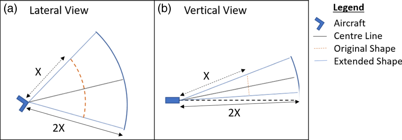
To cater for different conflict time scenarios, the shape can consist of two main profiles; an extended one by a larger factor and a unit factor. This is shown in Figure 2 for both lateral and vertical views. In Figure 2, X represents the current ground speed and heading of the aircraft, while 2X corresponds to an extended factor of twice the speed. Ground speed is used as it is a direct information source from the radar screen for ATCO monitoring tasks. An extension of X is used as ATCOs tend to project the traffic situation in tactical monitoring (Endsley and Garland, Reference Endsley and Garland2000; Endsley, Reference Endsley2011). A choice of 2 is used for the illustration of this concept.
(a, b) Extended Shape of aircraft.

3.2. Traffic complexity Conflict Activity Level (CAL) matrix
This phase comprises two main steps namely (a) pairwise evaluation and (b) establishment of a CAL matrix table.
3.2.1. Pairwise CAL evaluation
The first step seeks to evaluate the degree of traffic complexity via CAL between an aircraft pair within a specified Region(s) Of Interest (ROI). A ROI is a user-defined region that maps out a certain area under ATC review or surveillance within the radar display, which can vary in location, shape and size. In this work, the ROI is a circle with a point location centre. Through a series of commonly used Boolean algebra operations and location co-ordinates over a spatial volume, the proposed approach computes and determines the degree of overlap between the aircraft pair based on their corresponding 3D conflict shape movements. An overlap occurs whenever the flight conflict shape movement of the aircraft pair intersects due to their respective lateral and vertical trajectories. As opposed to 3D volumetric analysis, this approach was selected as it has the potential to perform quick and straightforward computation of complexity.
In this work, the degree of overlap is represented by four CALs having a score ranging from 0 to 3. A score of “0” indicates the least complexity as no aircraft is present. A score of “1” indicates low complexity which registered the presence of an aircraft pair but with totally no overlap in the 3D aircraft shape movement. Viewed from either a lateral or vertical plane perspective, one of its views would not have any overlap. A score of “2” indicates high complexity as an overlap is present in the 3D aircraft shape movement. These instances would either be partial overlap of aircraft shape movement at both lateral and vertical view planes at any angle and orientation, or a total overlap of aircraft shape movement in the lateral view plane with a partial overlap at any angle and orientation at the vertical view plane or vice versa. If the score is “3”, this indicates the highest complexity as the 3D aircraft shape movement of one aircraft is wholly inside the other in both lateral and vertical view planes.
3.2.2. Establishment of CAL matrix table
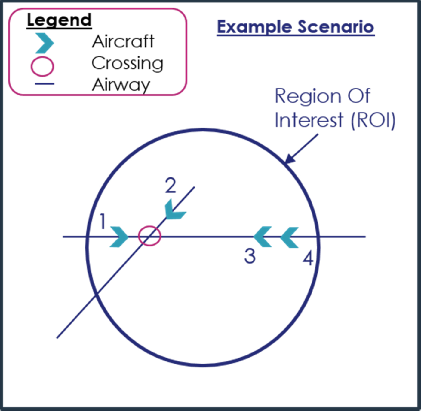
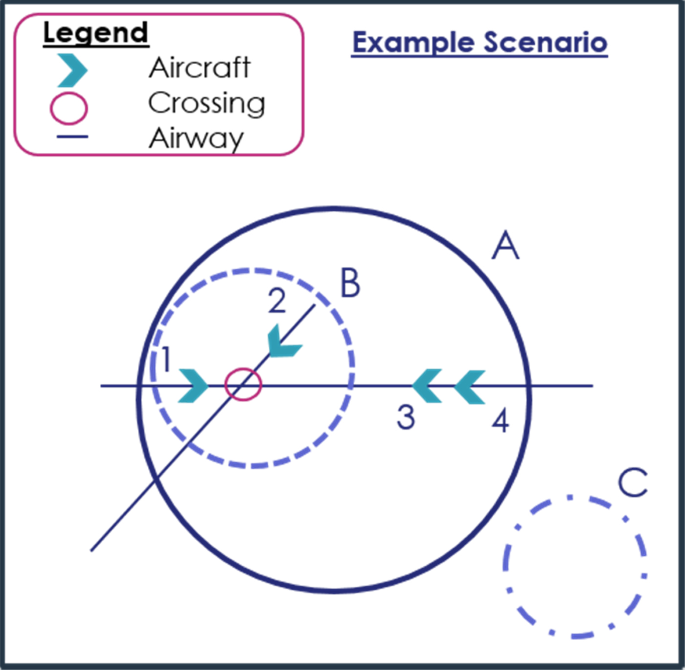
The second step is to establish the CAL matrix table which represents a compilation of various CAL scores for the different aircraft pairs within the specified ROI at an instance. This is as highlighted in Figure 3 where four aircraft are found to be randomly distributed on the radar at a particular time frame. Each aircraft is assigned a label number ranging from 1–4. The different parameters of individual aircraft are shown in Table 2.
Example scenario - a set of four aircraft registered in a radar at a particular time frame.

The Set of Aircraft Operating Parameters used in the example scenario.

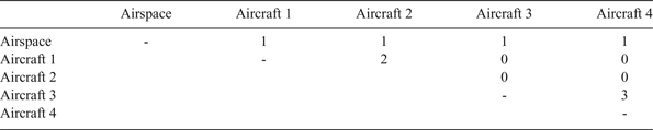
Based on a pairwise evaluation and mapping of these aircraft to the traffic complexity CALs, the pairing CAL scores can be tabulated into a matrix for the ROIs, as shown in Table 3. From Table 3, the approach can identify that the aircraft pairing 3 and 4 is at the highest complexity CAL of 3. In this instance, aircraft 3 is found to be wholly inside the shape movement of aircraft 4 both laterally and vertically, as aircraft 4 is climbing past the cruising FL of aircraft 3 at a higher speed. Immediate attention is therefore needed. A CAL of 2 is observed between aircraft pairing 1 and 2, as the 3D shape movement between aircraft pairing 1 and 2 has a partial overlap laterally and a total overlap vertically, therefore requiring some degree of monitoring.
CAL matrix table in example scenario from the pairwise aircraft comparison.

3.3. Overall complexity ROI score
The overall traffic complexity within a specified ROI is assessed in, (a) a static time frame (b) dynamically across multiple time frames.
3.3.1. Static traffic complexity at a particular time frame
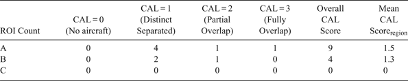
Traffic complexity in static time frames can be performed at different ROIs. Figure 4 shows a scenario of a set of four aircraft with three ROIs indicated. The overall CAL score and its mean for the different ROIs (A–C) for the three ROIs can be found in Table 4. Equations (1) and (2) are used to compute these CAL values.
Example scenario - a set of four aircraft having three different ROIs at a particular time frame.

Breakdown number of CAL scores in the example scenario.

From Table 4, one can observe that the overall CAL score and mean CAL score in ROI(A) is the highest and ROI(C) the lowest. A higher score denotes greater complexity in a given traffic scenario leading to a higher level of conflict being encountered. This is within expectations as aircraft in ROI(A) operate at a higher CAL score than ROI(C) with no aircraft in it. Besides this, when comparing ROI(A) and ROI(B), the higher complexity CAL in ROI(A) is due to aircraft 3 and 4 lying outside of ROI(B) and operating at a higher CAL. Flight adjustment may need to be made between this aircraft pair where appropriate. From the analysis, the approach is able to readily highlight the critical ROI to the ATCOs, thereby enabling them to better focus their tasks at hand.
 $$\eqalign{& {\rm Overall\,CAL\,Score} = \sum Total\,Number\,of\,Overlap\,Countsin\,CAL(i) * CAL\,Score(i), \cr & {\rm where}\;{\rm i} = 0,1,2,3.} $$
 $${\rm Mean\,CAL\,Scor}{\rm e}_{{\rm region/overall}} = \displaystyle{{{\rm Overall\,Complexity\,Score}} \over {Number\,of\,Overlap\,Counts_{region/overall}}}$$
3.3.2. Dynamic traffic complexity across multiple time frames
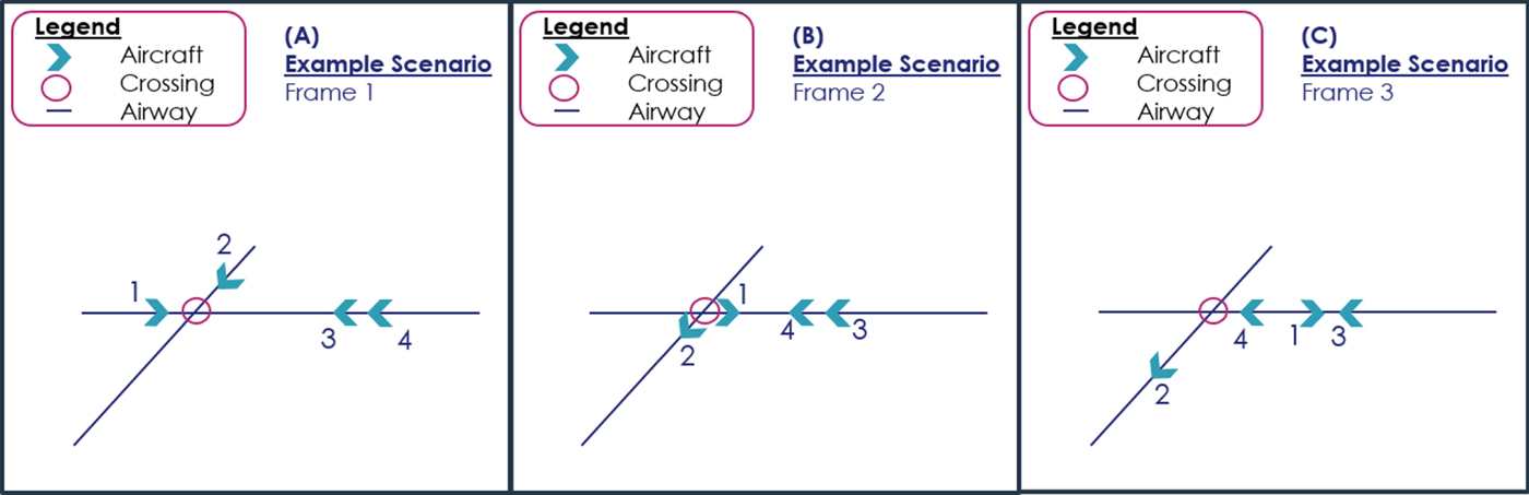
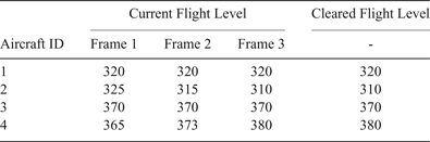
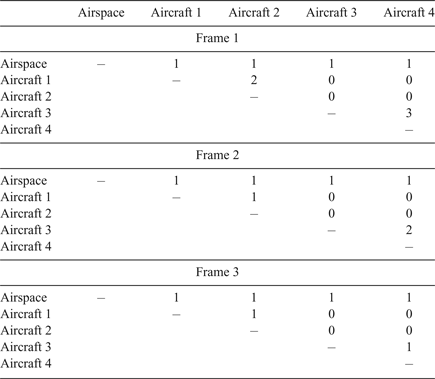
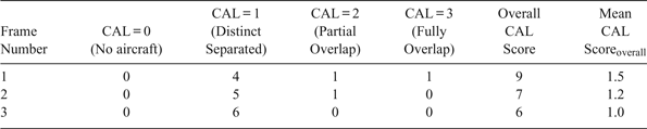
For dynamic traffic complexity analysis, simulation was performed on the four aircraft across the point crossing at three different time frames, as highlighted in Figure 5. Table 5 denotes the variations in the current FL (vertical profile) of the four aircraft at three time frames. Performing the CAL calculations, the pairwise CAL score matrix table for aircraft pairs, overall CAL and mean CAL scores for the whole scenario over the three time frames are shown in Tables 6 and 7.
Illustration of air traffic picture across three frames.

Changes in aircraft parameters across time.

Frame 1 CAL matrix table based on pairwise aircraft evaluation.

Breakdown number of CAL and overall complexity scores across time frames.

From Tables 6 and 7, it can be observed that at frame 1, higher complexity is registered owing to aircraft pair 1 and 2 heading towards the crossing point and aircraft pair 3 and 4 having a conflict separation issue between them. In frame 2, as aircraft pair 1 and 2 passed the crossing, the mean CAL score drops, as there is no overlap between the shape movement of 1 and 2 laterally. Moreover, aircraft pair 3 and 4 remains in CAL 3. However, in frame 3, this CAL score of 3 is absent. This indicates that aircraft pair 3 and 4 is distinctly separated, as there is no overlap of shape movement both laterally and vertically, due to the change in aircraft 4's flight movement between frames 2 and 3. As mentioned earlier, the ATCO's taskload is a function of traffic complexity. Hence, if one can simply sum up the scores across a duration of time, one can obtain a gauge of the taskload that an ATCO will likely undertake at a designated ROI. This could also be used as a new comparative taskload measure when comparing with other ROIs.
4. EXPERIMENTAL SETUP
An experimental setup was designed to test the CAL concept. A real-time simulator, the Nationaal Lucht-en Ruimtevaartlaboratorium (NLR) ATM Research SIMulator (NARSIM), was used to simulate various air traffic scenarios in real time. Aircraft position data, current and future flight trajectory data were extracted and used to compute the CAL complexity score tactically, by using a real-time post processing server (Wee et al., Reference Wee, Lye and Pinheiro2016; Wee et al., Reference Wee, Lye and Pinheiro2017a; Reference Wee, Trapsilawati, Lye, Chen and Pinheiro2017b).
To test and validate the concept of CAL, traffic scenarios were simulated and experimental tests were conducted using the setup described. Discussion of this concept test validation is made in the next section.
5. CONCEPT TEST VALIDATION
For the proposed CAL complexity model, validations were carried out for various traffic scenarios and then compared at factor analysis and model analysis levels.
5.1. Factor analysis level validation of proposed CAL complexity model
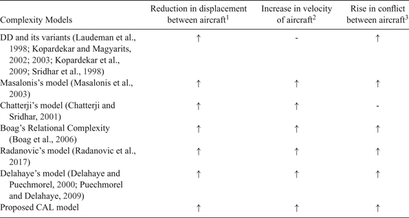
A factor analysis level validation of the proposed CAL complexity model with other complexity models is discussed in this section. Table 8 shows three commonly used factors found in these approaches to evaluate traffic complexity within a designated airspace. Assuming all other factors remain constant, a reduction in displacement between aircraft, an increase in aircraft speed or an increase in conflict risk between aircraft were found to result in greater traffic complexity. A “-” sign indicates that the approach did not account for this factor. Like all the other complexity models, the proposed CAL model registered similar trends, as seen in the change of complexity level in all three factors studied.
Outcome of Traffic Complexity Model Output due to changes in the key factors.

1 Reduction in displacement between aircraft indicates that the aircraft are closer to each other in the airspace.
2 Increase in velocity of aircraft indicates that the aircraft are flying at an increased speed.
3 Rise in conflict between aircraft indicates that there is an increase in conflict configuration among aircraft in the airspace.
5.2. Model analysis validation of proposed CAL complexity model
On model analysis, the proposed CAL complexity model was compared with Delahaye and Puechmorel's (Reference Delahaye and Puechmorel2000) model, one of the most compliant models, using a set of traffic scenarios. As these scenarios showcase the aircraft's intent as well as presented instances across a broad spectrum of air traffic situations, only a comparison with Delahaye and Puechmorel's (Reference Delahaye and Puechmorel2000) model is made in this paper. Such information was not available or evident in the approaches by Boag et al. (Reference Boag, Neal, Loft and Halford2006) and Chatterji and Sridhar (Reference Chatterji and Sridhar2001).
5.2.1. Description of traffic scenarios
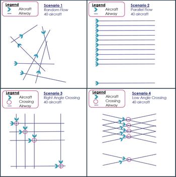
Four sample traffic scenarios were used for the calculation of complexity:
Scenario 1: A random flow of air traffic, consisting of 40 aircraft with random initial position and velocity was generated. In this work, only one random scenario was studied and used as an illustration. Further studies of aircraft flying in random trajectories which may result in a variation of CAL score will be presented in a further paper.
Scenario 2: A parallel flow of air traffic, consisting of 40 cruising aircraft at the same FL, moving in the same direction.
Scenario 3: A right angle crossing air traffic flow, consisting of 40 aircraft crossing at waypoints with intersecting lateral and vertical trajectories, inducing conflict.
Scenario 4: A low angle crossing of 15° (between the low angle range of 1° to 15°) air traffic flow, consisting of 40 aircraft crossing at waypoints with intersecting lateral and vertical trajectories, inducing conflict (Eurocontrol, 1997).
These scenarios are based on those highlighted in Delahaye and Puechmorel's (Reference Delahaye and Puechmorel2000) work to perform complexity computation. The geometric representations of the scenarios are also illustrated in Figure 6. In their work, complexity values were only computed based on the initial position and velocity at the start of each scenario.
Illustration of Validation Scenario.

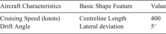
For all the scenarios, the traffic was assumed to be moving in a regular, orderly manner, using the same aircraft type. Airways constructed in the scenario observed the RNP10 navigation standard. Other fixed parameters that affect CAL shape are listed in Table 9, where the drift angle of the aircraft while cruising is set at 5° (Krajček et al., Reference Krajček, Nikoliæ and Domitroviæ2015).
Fixed parameters of aircraft's shape.

5.2.2. Model analysis validation results of proposed CAL complexity model
To validate the proposed CAL complexity model, the overall and mean complexity scores of the CAL model are used for comparison with other established models owing to the amount of information available in the cited papers.
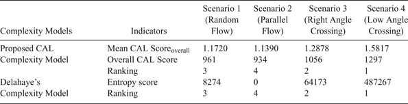
For the proposed CAL complexity model, overall and mean CAL scores are calculated for the four different traffic scenarios, using initial position and velocity at the start of the scenario (frame 1). The overall and mean CAL score at frame 1, together with its corresponding rank from highest to lowest (4 to 1) for each of the four scenarios are shown in Table 10. The results are consistent with those of Delahaye and Puechmorel (Reference Delahaye and Puechmorel2000) who ranked the four scenarios in descending order of complexity as low angle crossing, right angle crossing, random flow and parallel flow, as seen in Table 10.
Complexity model and complexity score comparison of all four scenarios at frame 1.

6. CONCLUSION
A new complexity calculation method, CAL, for overall and regional score, based on user specified input location and time, has been presented. CAL can determine the level of complexity pending on the state of overlap from the spatial shapes of individual aircraft defined in the airspace, with high resolution.
Tactical, instantaneous calculation can be performed at every time frame, thus allowing any slight deviation or change to be tracked more accurately. Critical regions on the radar screen can also be identified. A trend analysis of complexity can also be performed with historical data, to track the periods of high and low complexity. Hence, any sudden changes in complexity can be identified and isolated for further analysis of the exogenous traffic movements.
Test validation of CAL analysed at factor level indicates that the proposed CAL model is consistent with other established complexity models. At model level, validation of CAL with Delahaye's complexity model for the complexity score highlights that both models produce the same complexity ranking order over a range of air traffic scenarios.
The proposed approach is able to perform real time dynamic traffic complexity evaluation which could serve as a useful planning tool in allocation and duration of shift duties to ATCOs. Risk assessment and analysis in designated spatial areas can also be performed as well as identified regions of high traffic complexity. Nevertheless, the proposed method may be constrained by the number of aircraft within a particular ROI. This may make it difficult for ATCOs to define the exact ROI for complexity evaluation particularly if one is dealing with an unfamiliar airspace sector for the first time. This challenge can, however, be mitigated through experience in consultation with more senior ATCOs.
ACKNOWLEDGEMENTS
This research is funded by Thales Solutions Asia Pte Ltd, under the Economic Development Board, Industrial Postgraduate Programme, with Nanyang Technological University, Singapore. The authors would like to acknowledge and thank the staff at Thales Air System SAS, Thales Solutions Singapore and Air Traffic Management Research Institute of Nanyang Technological University, Singapore for their contributions and support towards this work.