The interaction between rotationally oscillating spheres and solid boundaries in a Stokes flow

F. Box; K. Singh; T. Mullin

doi:10.1017/jfm.2018.354

The interaction between rotationally oscillating spheres and solid boundaries in a Stokes flow

Published online by Cambridge University Press: 26 June 2018

F. Box

K. Singh and

T. Mullin

Show author details

F. Box*: Affiliation:
Manchester Centre for Nonlinear Dynamics, School of Physics and Astronomy, University of Manchester, Manchester M13 9PL, UKMathematical Institute, University of Oxford, Oxford OX2 6GG, UK
K. Singh: Affiliation:
Oxford Centre for Collaborative Applied Mathematics, Mathematical Institute, University of Oxford, Oxford OX2 6GG, UK
T. Mullin: Affiliation:
Manchester Centre for Nonlinear Dynamics, School of Physics and Astronomy, University of Manchester, Manchester M13 9PL, UKMathematical Institute, University of Oxford, Oxford OX2 6GG, UK
*: †Email address for correspondence: finn.box@maths.ox.ac.uk

Article contents

Abstract
Introduction
A model of a driven sphere oscillating in a viscous fluid
Experimental set-up
Results
Conclusions
References

Rights & Permissions

Abstract

We present the results of an experimental and theoretical investigation into the influence of proximate boundaries on the motion of an rotationally oscillating sphere in a viscous fluid. The angular oscillations of the sphere are controlled using the magnetic torque generated by a spatially uniform, oscillatory magnetic field which interacts with a small magnet embedded within the sphere. We study the motion of the sphere in the vicinity of stationary walls that are parallel and perpendicular to the rotational axis of the sphere, and near a second passive sphere that is non-magnetic and free to move. We find that rigid boundaries introduce viscous resistance to motion that acts to suppress the oscillations of the driven sphere. The amount of viscous resistance depends on the orientation of the wall with respect to the axis of rotation of the oscillating sphere. A passive sphere also introduces viscous resistance to motion, but for this case the rotational oscillations of the active sphere establish a standing wave that imparts vorticity to the fluid and induces oscillations of the passive sphere. The standing wave is analogous to the case of an oscillating plate in a viscous fluid; the amplitude of the wave decays exponentially with radial distance from the surface of the oscillating sphere. The standing wave introduces a phase lag between the motion of the active sphere and the response of the passive sphere which increases linearly with separation distance.

JFM classification

Low-Reynolds-number flows: Low-Reynolds-number flows

Information

Type: JFM Papers
Information: Journal of Fluid Mechanics , Volume 849 , 25 August 2018, pp. 834 - 859
DOI: https://doi.org/10.1017/jfm.2018.354 [Opens in a new window]
Copyright: © 2018 Cambridge University Press

1 Introduction

The interactions between spherical particles moving in a viscous fluid and nearby solid boundaries are key to understanding the physical processes associated with particle suspensions in a fluid (Happel & Brenner Reference Happel and Brenner1983; Kim & Karrila Reference Kim and Karrila1991). Fluid suspensions are confined by, and move along, rigid boundaries in a wide range of industrial applications. Examples include the manufacturing of paints and polymer suspensions, the measurement of rheological properties of colloidal suspensions (Cichocki et al. Reference Cichocki, Felderhof, Hinsen, Wajnryb and Blawzdziewicz1994) and the development of rotating sphere viscometers (Besseris, Miller & Yeates Reference Besseris, Miller and Yeates1999). In nature, particle–boundary interactions are key to the process of sedimentation induced by turbidity currents (Guazzelli & Hinch Reference Guazzelli and Hinch2010). In biological systems, fluid dynamic interactions are responsible for biofilms that are formed by the agglomeration of microorganisms near rigid walls and at air–liquid interfaces (Lauga & Powers Reference Lauga and Powers2009).

Studies on isolated, steady rotating spheres in a viscous fluid indicate that the surrounding fluid moves in concentric shells around the sphere with a speed that decays inversely with radial distance from the sphere centre (Buchanan Reference Buchanan1891; Jeffery Reference Jeffery1915; Lamb Reference Lamb1932; Kestin & Persen Reference Kestin and Persen1954). The presence of a nearby, stationary boundary modifies this flow field and suppresses the rotational motion (Happel & Brenner Reference Happel and Brenner1983). Moreover, the orientation of the axis of rotation of the sphere with respect to the wall has a significant impact on the resulting flow field.

For a sphere rotating steadily about an axis perpendicular to a nearby wall a resistive torque arises because of the no-slip condition at the wall and this in turn exerts an additional force on the sphere by the fluid. This wall-induced correction to the viscous torque increases as the sphere is brought closer to the wall (Jeffery Reference Jeffery1915). For a sphere that is sufficiently far from the wall, the torque scales as the cube of the separation distance (Liu & Prosperetti Reference Liu and Prosperetti2010) whereas when the sphere is very close to the wall lubrication effects become important and the torque scales as the inverse logarithm of the separation distance (Cox & Brenner Reference Cox and Brenner1967; Kim & Karrila Reference Kim and Karrila1991) and becomes infinite in the limit where the sphere touches the wall.

For a steady rotating sphere with its axis of rotation parallel to the wall once again a resistive torque is exerted on the sphere that increases as the separation distance between the wall and sphere is reduced (Dean & O’Neill Reference Dean and O’Neill1963; Goldman, Cox & Brenner Reference Goldman, Cox and Brenner1967). Far from the wall, the torque scales with the cube of the inverse separation distance, whereas very near the wall the torque decreases logarithmically with inverse separation distance. Viscous effects also result in a force that has components parallel and perpendicular to the wall. The parallel component originates from viscous shear and causes the sphere to translate in the direction that an untethered sphere would roll along the wall (Liu & Prosperetti Reference Liu and Prosperetti2010). Note that by the reciprocal theorem (Happel & Brenner Reference Happel and Brenner1983), a force generated by a sphere rotating near a boundary is analogous to the torque experienced by a sphere translating near a boundary (Faxén Reference Faxén1922; Ambari, Gauthier-Manuel & Guyon Reference Ambari, Gauthier-Manuel and Guyon1984). The component perpendicular to the wall arises from the pressure generated by the fluid layer squeezed between the sphere and the wall. This force is repulsive, forcing the sphere away from the boundary, is greater at smaller separations and decreases rapidly with increasing separation (Liu & Prosperetti Reference Liu and Prosperetti2010).

The linearity of the Stokes equations permits analytical treatment, in particular for simplified boundary conditions. More generally, the symmetry of spheres has been effectively exploited to develop a range of theoretical methods depending upon the configuration. The interaction between two spheres moving with equal velocity in a viscous fluid, along a line joining their centres, was first considered by Stimson & Jeffrey (Reference Stimson and Jeffrey1926). More recently considerable theoretical work has been performed on both the forward problem of linear and angular rate of change of momentum balance for prescribed motion, as well as the inverse problem to solve the motion at prescribed force and torque. These problems require a derivation of the resistance and mobility functions respectively to define the corresponding equations (Jeffrey & Onishi Reference Jeffrey and Onishi1984a ,Reference Jeffrey and Onishi b ; Kim & Miffin Reference Kim and Miffin1985; Cichocki, Felderhof & Schmitz Reference Cichocki, Felderhof and Schmitz1988; Jeffrey Reference Jeffrey1992). The method of reflections has been used to iteratively solve for interacting spheres in a viscous fluid, and yields accurate solutions for a sufficiently small number of arbitrarily shaped particles as long as they are far apart. As these particles approach each other the number of higher-order terms required to yield accurate solutions becomes prohibitively large. Multipole expansion methods can be used for solving for a finite number of closely spaced, interacting axisymmetric particles (Jeffery Reference Jeffery1915; Kim & Karrila Reference Kim and Karrila1991). However for problems that extend beyond these finite realms, an effective and versatile numerical approach is possible with boundary element methods that use singularity solutions to the Green’s function for Stokes equations. Pertinent to the problem studied in this paper is the steady rotating sphere that is represented by a spinning rotlet, and analytical solutions of a sphere near a rigid boundary were determined using the method of images by Blake & Chwang (Reference Blake and Chwang1974). In the context of unsteady Stokes flows, Pozrikidis (Reference Pozrikidis1989) used singularity methods to analyse oscillating spheres in a viscous fluid. For more complex configurations, boundary element methods lend themselves well to numerical treatment, where the complexity refers to particle shape as well as to the numbers of interacting particles. Moreover they can be effectively combined with analytical methods, such as the method of reflections (Kim & Russel Reference Kim and Russel1985; Ardekani & Rangel Reference Ardekani and Rangel2006) or the application of lubrication theory, which permits estimation of the leading contribution to the relative motion of a sphere near a boundary (Kim & Karrila Reference Kim and Karrila1991). Such theoretical techniques have been validated in experimental studies of the steady rotational motion of micron-sized colloidal particles controlled by optical tweezers (Crocker Reference Crocker1997; Meiners & Quake Reference Meiners and Quake1999; Henderson, Mitchell & Bartlett Reference Henderson, Mitchell and Bartlett2001, Reference Henderson, Mitchell and Bartlett2002; Trankle, Speidel & Rohrbach Reference Trankle, Speidel and Rohrbach2012), and therefore provide an accurate means of modelling the behaviour of multi-body configurations of rotating spheres.

One of our long-term goals is to model systems that comprise chains of oscillating spheres. Specifically it has been shown that arrays of rotationally oscillating spheres connected together via flexible filaments deform in a non-reciprocal manner and self-propel in a viscous fluid (Box et al. Reference Box, Han, Tipton and Mullin2017). In this way they act as configurable synthetic swimmers or micro-fluidic pumps. To this end, we develop an accurate, fast and robust numerical model that provides a foundation for modelling such complex, versatile motion in a viscous fluid.

Here, we progress the understanding of the fundamental fluid dynamics of rotationally oscillating spheres in the presence of solid boundaries. In doing so, we use the novel experimental technique of Box, Thompson & Mullin (Reference Box, Thompson and Mullin2015) to magnetically induce torsional oscillations in a sphere in a viscous fluid. The controlled oscillations are operated at constant driving torque and we refer to the sphere which moves in response to the magnetic field as ‘active’. We first consider active spheres near planar walls to understand the role of stationary boundaries on the response of the sphere. We then extend the approach to interactions between two untethered, moving spheres of non-negligible radius, one of which is ‘active’ and the other is ‘passive’ since it is non-magnetic and moves in response to changes in the flow field induced by the driven sphere.

This manuscript is organised as follows: In § 2 we apply the model for a driven sphere performing torsional oscillations in a viscous fluid near rigid boundaries, based on which we extend the model to consider sphere-pair interactions. The experimental set-up in which we control the motion of the sphere and measure the fluid and sphere interactions is described in § 3. A comparison between the model and the experiments is presented in § 4. Finally, the findings of this study are summarised and discussed in § 5.

2 A model of a driven sphere oscillating in a viscous fluid

A sphere oscillating in a fluid imparts its momentum to the surrounding fluid. We focus on spheres performing angular oscillations near rigid and movable boundaries in a viscous fluid. A few key assumptions are made here. Firstly, that the rate of change of fluid motion compared to the diffusion of vorticity is small, such that analytical progress may be made through linearisation of the Navier–Stokes equations. Secondly, we assume that the oscillations are of sufficiently low frequency that the flow can be treated as quasi-steady, such that the inertia of the fluid and a (neutrally buoyant) sphere can be neglected.

In this section we present the theoretical model where the singularity solutions from Blake & Chwang (Reference Blake and Chwang1974) for steady spinning spheres near boundaries are applied to the singularity method developed by Pozrikidis (Reference Pozrikidis1989) for oscillating spheres in a Stokes flow. The approach has been to develop a simple, robust, fast and sufficiently accurate method that models the dominant effects observed in the experiments. In § 2.1 we consider the theory for the flow field generated by a rotationally oscillating sphere. In § 2.2 we model the rotating sphere near rigid walls, and in § 2.3 we extend the model to predict the interaction between an oscillating active sphere and a second passive sphere.

2.1 Oscillating sphere in a Stokes flow

We consider an isolated sphere, of radius $a$ , with an embedded magnetic dipole pair, driven to oscillate with frequency omega in a viscous fluid (dynamic viscosity $\unicode[STIX]{x1D707}$ ) by application of an external magnetic field. The sphere is neutrally buoyant so we may neglect gravity and instead find that the contributions to the torque balance come from the viscous torque, $\boldsymbol{T}_{v}=-8\unicode[STIX]{x03C0}\unicode[STIX]{x03BC}a^{3}\,(\text{d}\unicode[STIX]{x1D703}/\text{d}t)\boldsymbol{e}_{k}$ (where $\boldsymbol{e}_{k}$ is the sphere’s oscillation axis) and magnetic torque, $\boldsymbol{T}_{m}=\boldsymbol{B}(t)\wedge \boldsymbol{m}$ . In an alternating magnetic field, $\boldsymbol{B}=B_{0}\exp (\text{i}\unicode[STIX]{x1D714}t)\boldsymbol{e}_{i}$ (acting along direction $\boldsymbol{e}_{i}$ , $\text{i}=\sqrt{-1}$ ), the magnetic sphere dipole moment $\boldsymbol{m}=m(\sin \check{\unicode[STIX]{x1D703}}\boldsymbol{e}_{i},\cos \check{\unicode[STIX]{x1D703}}\boldsymbol{e}_{j})$ , where $m$ is the magnetic dipole strength, $\check{\unicode[STIX]{x1D703}}=\bar{\unicode[STIX]{x1D703}}+\unicode[STIX]{x1D703}(t)$ , $\unicode[STIX]{x1D703}(t)$ is the time-varying angular component about the mean dipole orientation axis, $\bar{\unicode[STIX]{x1D703}}$ , 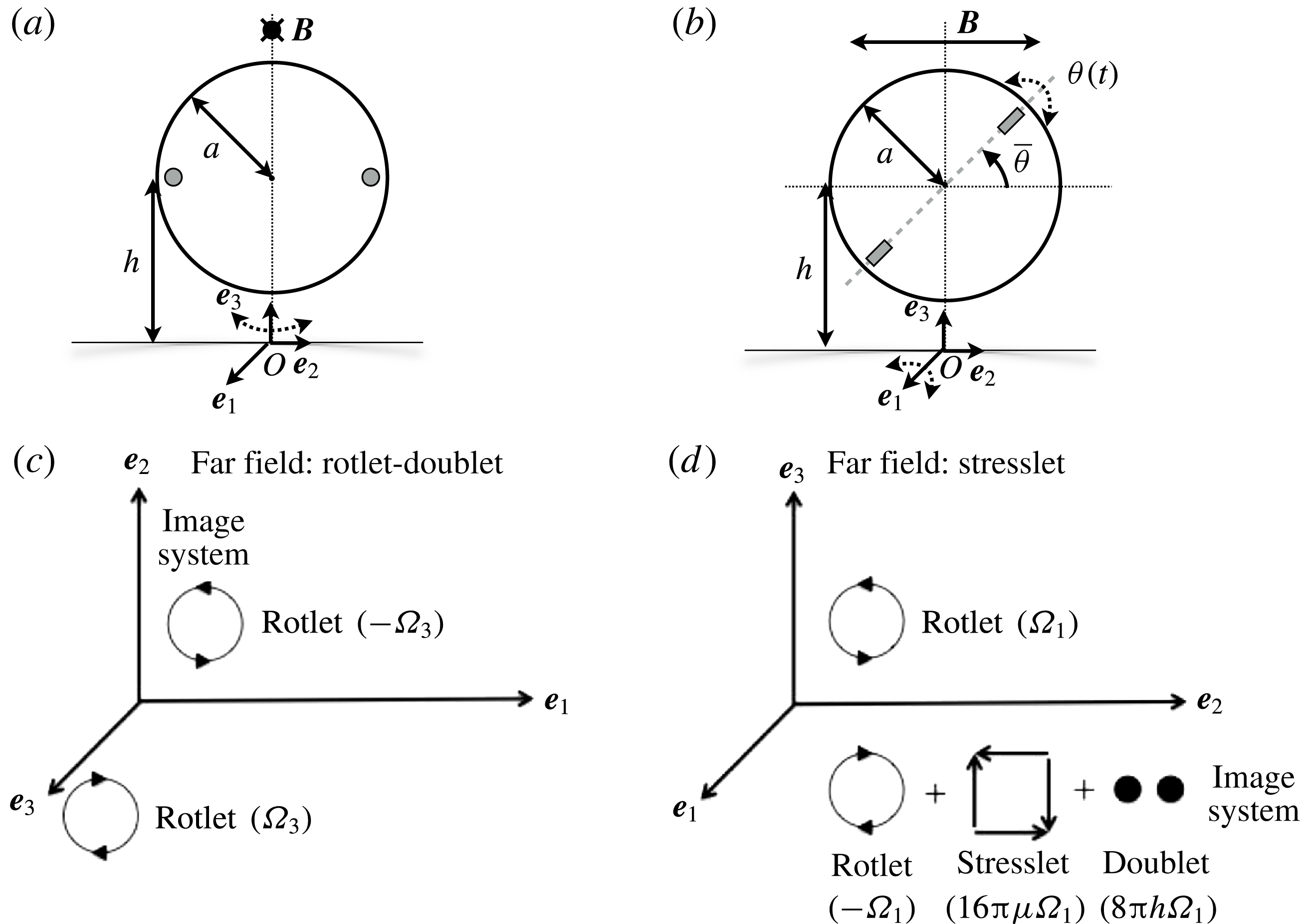depicted in figure 1(b). Furthermore $[i,j,k]\in [1,2,3]$ refer to the coordinate axes, the particular combination of which depends upon the rotation and wall orientation axes and are specified for the cases considered later in this section (also see figure 1). The torque balance equation reduces to:

(2.1)

$$\begin{eqnarray}\frac{\text{d}\unicode[STIX]{x1D703}(t)}{\text{d}t}=-\frac{B_{0}m}{8\unicode[STIX]{x03C0}\unicode[STIX]{x03BC}a^{3}}\sin \check{\unicode[STIX]{x1D703}}\text{e}^{\text{i}\unicode[STIX]{x1D714}t}.\end{eqnarray}$$

The Mason number, $M_{a}=B_{0}m/(8\unicode[STIX]{x03C0}\unicode[STIX]{x03BC}a^{3}\unicode[STIX]{x1D714})\approx 8\gg 1$ so we may assume small angle oscillations (Box et al. Reference Box, Thompson and Mullin2015). This allows us to isolate magnetic forcing from the fluid dynamics by assuming that the sphere undergoes angular oscillations of amplitude $\unicode[STIX]{x1D703}_{0}$ , so

(2.2)

$$\begin{eqnarray}\unicode[STIX]{x1D703}(t)=\unicode[STIX]{x1D703}_{0}\exp (\text{i}\unicode[STIX]{x1D714}t).\end{eqnarray}$$

The viscous fluid surrounding the oscillating sphere can be modelled by the unsteady Stokes equations:

(2.3a,b )

$$\begin{eqnarray}\frac{\unicode[STIX]{x2202}\boldsymbol{U}}{\unicode[STIX]{x2202}T}=-\frac{1}{\unicode[STIX]{x1D70C}}\unicode[STIX]{x1D735}P+\unicode[STIX]{x1D708}\unicode[STIX]{x1D6FB}^{2}\boldsymbol{U},\quad \unicode[STIX]{x1D735}\boldsymbol{\cdot }\boldsymbol{U}=0,\end{eqnarray}$$

where $\boldsymbol{U}$ and $P$ are respectively the fluid velocity and pressure generated by the flow of fluid of density $\unicode[STIX]{x1D70C}$ , and viscosity $\unicode[STIX]{x1D708}$ . The characteristic length scale, $a$ (the radius of the driven sphere), and characteristic time scale, $1/\unicode[STIX]{x1D714}$ , are used to non-dimensionalise (2.3). Taking Fourier transforms of the momentum conservation equation gives

(2.4a,b )

$$\begin{eqnarray}(\unicode[STIX]{x1D6FB}^{2}+\text{i}\unicode[STIX]{x1D6FC})\hat{\boldsymbol{u}}=\unicode[STIX]{x1D735}\hat{p},\quad \unicode[STIX]{x1D6FC}=\frac{\unicode[STIX]{x1D714}a^{2}}{\unicode[STIX]{x1D708}},\end{eqnarray}$$

where $\hat{(.)}$ corresponds to the dimensionless Fourier transformed variables, and the Womersley number, $\unicode[STIX]{x1D6FC}$ , is the frequency parameter. The linearisation assumption used to derive the Stokes equations requires that $\unicode[STIX]{x1D6FC}\gg Re$ , which for a rotationally oscillating sphere given $U\sim \unicode[STIX]{x1D703}_{0}a\unicode[STIX]{x1D714}$ corresponds to a linear constraint on the angular rotation amplitude, $\unicode[STIX]{x1D703}_{0}\ll 1~\text{radian}$ ( ${\approx}57^{\circ }$ ). The correct length scale is the arc length traversed by a rotating sphere $\unicode[STIX]{x1D703}_{0}a$ . However as $\unicode[STIX]{x1D703}_{0}$ varies with separation distance from the boundary, we maintain $\unicode[STIX]{x1D703}_{0}$ as a variable, and retain the sphere radius as the characteristic length scale.

Figure 1.

(a,b) Schematic diagrams of a sphere of radius $a$ undergoing rotational oscillations about axes (a) $\boldsymbol{e}_{3}$ (perpendicular to the wall) and (b) $\boldsymbol{e}_{1}$ (parallel to the wall), respectively. The axis of rotation is indicated by the dotted, curved arrow. The applied external magnetic field vector lies along $\pm \boldsymbol{e}_{1}$ and $\pm \boldsymbol{e}_{2}$ in (a) and (b) respectively, the embedded magnets are depicted in grey, the dipole axis is the grey dashed line, the baseline dipole angle is $\bar{\unicode[STIX]{x1D703}}$ and the angular oscillation contribution is $\unicode[STIX]{x1D703}(t)$ . The spheres are distance $h$ from the wall, where the wall normal is along $\boldsymbol{e}_{3}$ . (c,d) Schematic diagrams illustrating the model for a rotating sphere, represented by a rotlet singularity, and the corresponding image system for a wall where the axis of rotation of the sphere lies (c) along $\boldsymbol{e}_{3}$ , perpendicular to, and (d) $\boldsymbol{e}_{1}$ , parallel to, the wall (Blake & Chwang Reference Blake and Chwang1974).

We follow Pozrikidis (Reference Pozrikidis1989) who used Green’s functions to find singular distributions to model the flow field near an oscillating sphere. For angular velocity $\bar{\unicode[STIX]{x1D74E}}\text{e}^{\text{i}t}=\unicode[STIX]{x1D703}_{0}\text{e}^{\text{i}t}\boldsymbol{e}_{3}$ a flow field is generated, which can be expressed in terms of distance $\boldsymbol{r}$ from the centre of the sphere:

(2.5)

$$\begin{eqnarray}\displaystyle \boldsymbol{u}(\boldsymbol{r},t) & = & \displaystyle \boldsymbol{u}_{s}u_{\unicode[STIX]{x1D706}}\text{e}^{\text{i}t}\end{eqnarray}$$

(2.6)

$$\begin{eqnarray}\displaystyle \text{where}\quad \boldsymbol{u}_{s}(\boldsymbol{r}) & = & \displaystyle \frac{\bar{\unicode[STIX]{x1D74E}}\wedge \boldsymbol{r}}{r^{3}}=\unicode[STIX]{x1D703}_{0}\left(\frac{-r_{2}\boldsymbol{e}_{1}+r_{1}\boldsymbol{e}_{2}}{r^{3}}\right),\end{eqnarray}$$

(2.7)

$$\begin{eqnarray}\displaystyle \text{and}\quad u_{\unicode[STIX]{x1D706}}(r) & = & \displaystyle \frac{1+\unicode[STIX]{x1D706}r}{1+\unicode[STIX]{x1D706}}\exp (\unicode[STIX]{x1D706}[1-r]).\end{eqnarray}$$

Note that $\boldsymbol{u}_{s}$ is the steady contribution resulting from a spinning rotlet of angular speed $\bar{\unicode[STIX]{x1D74E}}$ , $u_{\unicode[STIX]{x1D706}}\text{e}^{\text{i}t}$ is the oscillatory contribution and

(2.8)

$$\begin{eqnarray}\unicode[STIX]{x1D706}=(\unicode[STIX]{x1D6FC}/2)^{1/2}\exp [-\text{i}\unicode[STIX]{x03C0}/4].\end{eqnarray}$$

Equation (2.5) corresponds to the well-known result that a sphere oscillating in an unbounded fluid generates a standing wave in the radial direction with an amplitude that decays exponentially with distance from the sphere. This is termed a shear wave because the sphere imparts vorticity to the fluid; and the shearing fluid is propagated radially outwards from the moving sphere (Stuart Reference Stuart and Rosenhead1963).

2.2 Angular oscillations of a sphere near a wall

The flow field around the sphere is modified as the sphere is brought closer to a rigid wall. We examine two cases, in § 2.2.1 and § 2.2.2, where the axis of rotation of the sphere is parallel to and perpendicular to the wall normal respectively, as illustrated in figures 1(a) and 1(b) respectively. For both cases the wall lies in the plane $(\boldsymbol{e}_{1},\boldsymbol{e}_{2})$ , and the wall normal is aligned with $\boldsymbol{e}_{3}$ . A schematic diagram of the system of rotlet and image singularities that are required to represent the resulting flow fields (Blake & Chwang Reference Blake and Chwang1974) are shown in figure 1(c,d).

2.2.1 Flow induced by a sphere oscillating about an axis of rotation perpendicular to the wall

For this case the sphere positioned at $\unicode[STIX]{x1D743}=(0,0,h/a)$ , is modelled as a rotlet oscillating with its rotational axis perpendicular to the wall and of strength $\unicode[STIX]{x1D734}=\unicode[STIX]{x1D6FA}\boldsymbol{e}_{3}$ (as shown in figure 1 c), where

(2.9)

$$\begin{eqnarray}\unicode[STIX]{x1D6FA}(r,t;h)=\unicode[STIX]{x1D703}_{0}(h)u_{\unicode[STIX]{x1D706}}(r)\text{e}^{\text{i}t},\end{eqnarray}$$

and $r,t$ are spatial and temporal coordinates respectively, and $h$ is a controlled parameter. The method of images is used at the boundary to satisfy the no-slip condition and introduces a conjugate image rotlet positioned at $\unicode[STIX]{x1D743}^{\ast }=(0,0,-h/a)$ rotating in the opposite sense with strength $\unicode[STIX]{x1D734}^{\ast }=\unicode[STIX]{x1D6FA}^{\ast }\boldsymbol{e}_{3}$ , where:

(2.10)

$$\begin{eqnarray}\unicode[STIX]{x1D6FA}^{\ast }(r,t;h)=\unicode[STIX]{x1D703}_{0}(h)\frac{1+\unicode[STIX]{x1D706}^{\ast }r}{1+\unicode[STIX]{x1D706}^{\ast }}\exp [\unicode[STIX]{x1D706}^{\ast }(1-r)]\text{e}^{-\text{i}t},\end{eqnarray}$$

and $\unicode[STIX]{x1D706}^{\ast }=(\unicode[STIX]{x1D6FC}/2)^{1/2}\exp [\text{i}\unicode[STIX]{x03C0}/4]$ is the complex conjugate of $\unicode[STIX]{x1D706}$ as defined in (2.8).

We define $\boldsymbol{r}$ and $\boldsymbol{r}^{\ast }$ , respectively as the position vectors of an arbitrary fluid particle relative to the rotlet and its conjugate image rotlet, and $r_{i}=x_{i}-\unicode[STIX]{x1D709}_{i};i\in [1,3]$ , $r=|\boldsymbol{r}|$ (and $r_{i}^{\ast }=x_{i}-\unicode[STIX]{x1D709}_{i}^{\ast }$ , $r^{\ast }=|\boldsymbol{r}^{\ast }|$ ).

Finally the velocity induced in the fluid by the combined rotlet-and-image system defined in Cartesian space $\boldsymbol{x}=(x_{1},x_{2},x_{3})$ is given by,

(2.11)

$$\begin{eqnarray}\boldsymbol{u}_{\bot }(\boldsymbol{x},t;h)=\left(\frac{\unicode[STIX]{x1D6FA}(r,t;h)}{r^{3}(\boldsymbol{x}-\unicode[STIX]{x1D743}(h))}-\frac{\unicode[STIX]{x1D6FA}^{\ast }(r,t;h)}{{r^{\ast }}^{3}(\boldsymbol{x}-\unicode[STIX]{x1D743}^{\ast }(h))}\right)(-r_{2}\boldsymbol{e}_{1}+r_{1}\boldsymbol{e}_{2}).\end{eqnarray}$$

For simplicity we will henceforth drop the arguments for $r,r^{\ast }$ ; and the separation distance $h$ will be retained as a parameter.

2.2.2 Flow induced by a sphere oscillating about an axis of rotation parallel to the wall

For the case where the axis of rotation of the sphere is parallel to the wall normal, we model a rotlet of strength, $\unicode[STIX]{x1D734}=\unicode[STIX]{x1D6FA}(r,t;h)\boldsymbol{e}_{1}$ (see figure 1 d). The resulting fluid velocity field is given by

(2.12)

$$\begin{eqnarray}\boldsymbol{u}_{||}(\boldsymbol{x},t;h)=(0,u_{2},u_{3}),\end{eqnarray}$$

where

(2.13)

$$\begin{eqnarray}\displaystyle & \displaystyle u_{2}(\boldsymbol{x},t;h)=-\left(\frac{r_{3}\unicode[STIX]{x1D6FA}}{r^{3}}-\frac{\unicode[STIX]{x1D6FA}^{\ast }r_{3}^{\ast }}{{r^{\ast }}^{3}}\right)-2h\unicode[STIX]{x1D6FA}^{\ast }\left(\frac{1}{{r^{\ast }}^{3}}-\frac{3{r_{2}^{\ast }}^{2}}{{r^{\ast }}^{5}}\right)-6\unicode[STIX]{x1D6FA}^{\ast }\frac{{r_{2}^{\ast }}^{2}r_{3}^{\ast }}{{r^{\ast }}^{5}}, & \displaystyle\end{eqnarray}$$

(2.14)

$$\begin{eqnarray}\displaystyle & \displaystyle u_{3}(\boldsymbol{x},t;h)=\left(\frac{r_{2}\unicode[STIX]{x1D6FA}}{r^{3}}-\frac{\unicode[STIX]{x1D6FA}^{\ast }r_{2}^{\ast }}{{r^{\ast }}^{3}}\right)+6h\unicode[STIX]{x1D6FA}^{\ast }\frac{r_{2}^{\ast }r_{3}^{\ast }}{{r^{\ast }}^{5}}-6\unicode[STIX]{x1D6FA}^{\ast }\frac{r_{1}^{\ast }r_{2}^{\ast }r_{3}^{\ast }}{{r^{\ast }}^{5}}. & \displaystyle\end{eqnarray}$$

It may be noted that this configuration does not have a symmetric image system, and at $\unicode[STIX]{x1D743}^{\ast }=(0,0,-h/a)$ the image system comprises the conjugate image rotlet, a source doublet and a stresslet as given by Blake & Chwang (Reference Blake and Chwang1974) for a similar configuration in a steady Stokes flow, where $\unicode[STIX]{x1D6FA}$ and $\unicode[STIX]{x1D6FA}\ast$ correspond to the source strength for an unsteady oscillating rotlet and its conjugate as given by (2.9), (2.10) respectively. Therefore (2.13), (2.14) correspond to the flow field generated by an unsteady oscillating sphere, following the linearity and quasi-steady flow assumptions defined in the introduction of § 2.

2.2.3 Wall-induced suppression of rotation

In the model developed thus far the oscillations of the spheres are assumed to be quasi-steady. This assumption is a key aspect required to describe the motion of the pair of spheres, and is discussed in § 2.3. Conversely, for a sphere near a rigid wall, after the initial transients have settled, the oscillations of the sphere may be treated as essentially steady such that there is virtually no difference between the time-averaged and instantaneous velocity of a fluid particle near the sphere. Hence for the rigid wall case, with no loss of generality we may assume time independence in describing the motion of the sphere and fluid response.

Indeed the rigid wall suppresses the amplitude of oscillations of the sphere as it approaches the wall. Furthermore, as the separation distance reduces below a sphere radius, lubrication effects manifest as an increased suppression in angular amplitude. This is particularly evident for the parallel-wall case.

In order to estimate the impact of wall-induced suppression we first compute the velocity on the surface of the rotating sphere, $V_{s}$ . Since the oscillating rotlet has no inherent length scale, we estimate the velocity on the surface of the sphere by interrogating the flow field at a unit radial distance, $a$ , from the rotlet centre and calculate the equatorial angular-average value, given $\boldsymbol{x}=(0,\sin \unicode[STIX]{x1D717},h/a+\cos \unicode[STIX]{x1D717})$ , $\unicode[STIX]{x1D717}$ being the angle of a point on sphere surface in the equatorial plane. We denote $\unicode[STIX]{x1D703}_{\infty }$ to be the amplitude of the angular motion of the sphere far from the wall. Then the motion of a point on the sphere can be estimated by considering that the velocity of the sphere is the sum of the velocity far from the wall, $\unicode[STIX]{x1D714}a\unicode[STIX]{x1D703}_{\infty }$ , and the velocity perturbation from the wall, $\boldsymbol{u}(\unicode[STIX]{x1D717};h)$ given by (2.11) and (2.12) for the perpendicular and parallel wall cases respectively. The magnitude of the surface velocity may be estimated as:

(2.15)

$$\begin{eqnarray}\displaystyle \tilde{V}_{s}(h) & = & \displaystyle \unicode[STIX]{x1D714}a\unicode[STIX]{x1D703}_{0}(h)=\unicode[STIX]{x1D714}a\left(\unicode[STIX]{x1D703}_{\infty }-\int _{0}^{2\unicode[STIX]{x03C0}}|\boldsymbol{u}(\unicode[STIX]{x1D717};h)|\,\text{d}\unicode[STIX]{x1D717}\right)\end{eqnarray}$$

(2.16)

$$\begin{eqnarray}\displaystyle & = & \displaystyle V_{s}-\unicode[STIX]{x1D714}a\langle u(h)\rangle ,\end{eqnarray}$$

where $u=|\boldsymbol{u}|$ is the magnitude of the velocity of the sphere, and $\langle u\rangle$ indicates averaging in the equatorial plane. Finally, with the assumption of symmetry we consider the fluid velocity in the equatorial plane of the sphere, and hence estimate the amplitude of angular rotation as a function of wall separation distance, $h$ , to be

(2.17)

$$\begin{eqnarray}\frac{\tilde{V}_{s}}{a\unicode[STIX]{x1D714}}=\unicode[STIX]{x1D703}_{0}(h)=\unicode[STIX]{x1D703}_{\infty }-\langle u(h)\rangle .\end{eqnarray}$$

Thus $\unicode[STIX]{x1D703}_{0}(h)$ is the amplitude of rotation of the sphere when it is a distance $h$ from the wall, and $\unicode[STIX]{x1D703}_{0}/\unicode[STIX]{x1D703}_{\infty }\rightarrow 1$ as $\langle u\rangle \rightarrow 0$ or $\tilde{V}_{s}\rightarrow a\unicode[STIX]{x1D714}$ .

As the gap between the wall and the sphere decreases, wall effects become important and must be included to predict the response of the sphere. For the case where the rotation axis is parallel to the wall, following Kim & Karrila (Reference Kim and Karrila1991) we model the effect of the lubrication layer (detailed in appendix A) and thus derive an expression for the amplitude of sphere rotation,

(2.18)

$$\begin{eqnarray}\unicode[STIX]{x1D703}_{0,L}(h)=\unicode[STIX]{x1D703}_{\infty }\exp \left(-\frac{1}{M_{a}}\left[\frac{C_{0}}{1+{\mathcal{L}}(h)}-C_{\infty }\right]\right),\end{eqnarray}$$

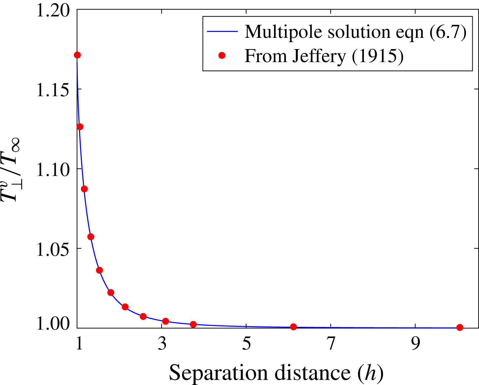
where ${\mathcal{L}}(h)$ is the lubrication contribution to the viscous torque, given by (A 3), $M_{a}$ is the Mason number and $C_{0},C_{\infty }$ are constants corresponding to the phase difference between the sphere oscillation and the alternating magnetic field for the near field and isolated sphere situation respectively, and are inferred from the experiments. For the perpendicular-wall case we use the accurate multipole solution derived by Jeffery (Reference Jeffery1915) to show the subtle contribution of the wall that is not accounted for by the rotlet model, given by (2.11) (see appendix A).

2.3 A sphere performing angular oscillations in the vicinity of another sphere

In this section we develop a model of a passive sphere placed in the vicinity of an actively oscillating sphere rotating about axis $\boldsymbol{e}_{1}$ , orthogonal to a line joining the centres of the spheres. The no-slip condition on the surface of the second sphere influences the resulting flow field, and we adopt the method developed for spheres oscillating about an axis of rotation parallel to nearby walls to model the motion of the fluid near the active and passive spheres.

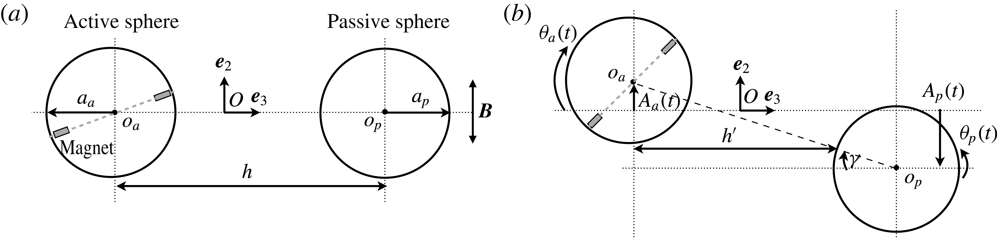
A schematic diagram of an active, oscillating sphere rotating near a passive sphere is shown in figure 2. The positions of the active and passive spheres are given by dimensionless coordinates $(0,x_{p,2},x_{p,3})$ and $(0,x_{a,2},x_{a,3})$ respectively, where $|x_{p,2}|=A_{p}/a_{a},|x_{a,2}|=A_{a}/a_{a}$ , and $A_{p}$ and $A_{a}$ are the amplitudes of translational oscillations along $\boldsymbol{e}_{2}$ for passive and active spheres respectively. Note that the positions of the spheres are assumed to be confined to their equatorial plane, so with no loss of generality $x_{p,1}=x_{a,1}=0$ .

Figure 2.

Schematic diagrams of the sphere pair, comprising an active sphere (radius $a_{a}$ , centre at $o_{a}$ ) and passive sphere (radius $a_{p}$ , centre at $o_{p}$ ) with the sphere centres $o_{a},o_{p}$ distance $h$ apart. The diagrams show the (a) initial undisturbed state and (b) instantaneous perturbed state when magnetically activated with active sphere centre to passive sphere wall distance $h^{\prime }(t)=h-a_{p}\cos \unicode[STIX]{x1D6FE}(t)$ . The active sphere rotates through angle $\unicode[STIX]{x1D703}_{a}$ about axis $\boldsymbol{e}_{3}$ , perturbing the surrounding fluid. The configuration results in induced rotation $\unicode[STIX]{x1D703}_{p}$ about $\boldsymbol{e}_{3}$ in the passive sphere, and translational motion $A_{a}(t)$ and $A_{p}(t)$ along $\boldsymbol{e}_{2}$ in the active and passive spheres respectively. The embedded magnets in the active sphere are indicated in the diagram and the dipole axis of the pair of magnets is depicted by the grey dashed line. The alternating magnetic field, $\boldsymbol{B}$ , acts along $\pm \boldsymbol{e}_{2}$ .

Two key differences distinguish the passive–active spheres from the sphere–wall case: firstly at an instant in time the passive sphere corresponds to a ‘curved wall’ with radius of curvature $a_{p}$ . Secondly the passive sphere moves in response to the flow field generated by the active sphere. We have developed an iterative numerical model to track the coupled motion of the sphere pair that accounts for these key aspects.

In the first step, the passive sphere is modelled as a curved moving boundary, where the instantaneous distance from the active sphere centre to the wall is given by

(2.19)

$$\begin{eqnarray}h^{\prime }(t;h)=h-a_{p}\cos \unicode[STIX]{x1D6FE}(t;h),\end{eqnarray}$$

where

(2.20)

$$\begin{eqnarray}\unicode[STIX]{x1D6FE}(t;h)=\tan ^{-1}\left(\frac{x_{p,2}(t;h)-x_{a,2}(t;h)}{h/a_{a}}\right)\end{eqnarray}$$

is the angle between two sphere centres, as indicated in figure 2. Note that the difference in distance between active and passive sphere walls, $a_{p}(1-\cos \unicode[STIX]{x1D6FE})$ , arises from the relative motion between translating spheres (of finite wall curvature). With no loss of generality $\unicode[STIX]{x1D6FE}(0;h)=0$ , corresponds to the initial condition where the centres of the spheres are aligned, as depicted in figure 2(a).

In the next step, we update the position of the active sphere, by calculating the velocity of the surface of the sphere. As the spheres are neutrally buoyant, we assume that the spheres move in response to the perturbed flow field, and hence the points on the sphere surface may be treated as a tracer particle in the fluid. The flow velocity for this configuration is given by (2.12). As in the previous section we can define the points on the sphere surface in polar coordinates, $\boldsymbol{x}=(0,\sin \unicode[STIX]{x1D717},h^{\prime }(t)/a_{a}+\cos \unicode[STIX]{x1D717})$ , where $\unicode[STIX]{x1D717}$ , is the equatorial angle of a point on the surface of the sphere. Next we integrate the equatorially averaged velocity $\langle u_{||}\rangle$ in time and compute the instantaneous position of the active sphere,

(2.21)

$$\begin{eqnarray}\displaystyle \boldsymbol{x}_{a}(t;h) & = & \displaystyle \int _{0}^{t}\int _{0}^{2\unicode[STIX]{x03C0}}\boldsymbol{u}_{||}(\unicode[STIX]{x1D717},t^{\prime };h)\,\text{d}\unicode[STIX]{x1D717}\,\text{d}t^{\prime }\nonumber\\ \displaystyle & = & \displaystyle \int _{0}^{t}\langle u_{||}(t^{\prime };h)\rangle \,\text{d}t^{\prime },\end{eqnarray}$$

where $\boldsymbol{u}_{||}(\boldsymbol{x},t)=(0,u_{2},u_{3})$ is given by (2.12)–(2.14).

In the final step we update the position of the passive sphere, by treating it as a tracer particle moving in the flow field induced by the rotlet, where the velocity at the centre of the passive sphere,

(2.22)

$$\begin{eqnarray}\boldsymbol{u}_{p}(t;h)=\frac{u_{\unicode[STIX]{x1D706}}\text{e}^{\text{i}t}}{r_{p}^{3}}\boldsymbol{r}_{p}(t;h),\end{eqnarray}$$

and $\boldsymbol{r}_{p}(t;h)=(0,r_{p,2},r_{p,3}),r_{p,i}(t;h)=x_{p,i}(t;h)-x_{a,i}(t;h),i\in [1,3]$ , is the vector distance between passive and active sphere centres and $u_{\unicode[STIX]{x1D706}}$ is given by (2.7). Finally we update the position of the passive sphere by integrating (2.22) in time, as for the active sphere in (2.21). For a given separation distance, $h$ , we solve for the passive and active sphere positions, until we achieve iterative convergence (the convergence criterion is set at $10^{-6}$ on the relative iteration error in sphere position). The main advantage of this approach is that it is a simple, fast and scalable method and yet is sufficiently accurate to capture the fundamental response of interacting spheres.

3 Experimental set-up

We actively controlled the rotational oscillations of a sphere in a viscous fluid using the application of external magnetic fields (Box et al. Reference Box, Thompson and Mullin2015). Driving the sphere in this way is a practical method which allows precise, non-contact control of the motion of the sphere and does not affect the local environment, so is suitable for miniaturisation and could be used in in vivo biomedical settings (Parkin et al. Reference Parkin, Knoner, Nieminen, Heckenberg and Rubinsztein-Dunlop2007). The technique has been used to control the motion of micron-sized, dipolar colloids known as Janus spheres (Steinbach, Gemmin & Erbe Reference Steinbach, Gemmin and Erbe2016) and enables insights into the fluid response and the feedback effects of the fluid on the motion of the sphere. Here, we performed the experiments at the macro-scale as it enabled quantitative measurement of the flow field which can be directly compared with the results from our theoretical model.

Cylindrical, neodymium magnets, of length $3.00\pm 0.01~\text{mm}$ and diameter $2.48\pm 0.01~\text{mm}$ , were carefully embedded into high-precision polypropylene spheres (Dejay Distribution Ltd., UK). Application of an external magnetic field exerted a torque on the embedded magnet causing the sphere to rotate. The number of embedded magnets depended on the size of the spheres; two were positioned diametrically opposite and flush with the surface in spheres of diameter $2a=15.86\pm 0.01~\text{mm}$ , whereas one was positioned in the centre of spheres of $2a=12.70\pm 0.01~\text{mm}$ . In both cases, the magnets occupied less than 2 % of the volume of the sphere. In the case of the larger sphere, the adjacent poles of the two magnets were placed opposite one another such that the two magnets acted as a single dipole.

The polypropylene spheres were less dense than the fluid and therefore, after the inclusion of magnets, additional non-magnetic weights were embedded in the spheres in order to attain a close approximation to neutral buoyancy in the fluid. The resulting average density of the spheres was $979.97\pm 5.64~\text{kg}~\text{m}^{-3}$ (with respect to the fluid density the density of the spheres was $1.004$ and, as such, buoyancy effects were negligible). The orientation of the magnetic dipole of the sphere was controlled, in the absence of an applied field, by careful positioning of the embedded weights such that the magnetic dipole axis of the sphere was orientated orthogonal to the applied field direction. The embedding of magnets and weights in the spheres resulted in a non-uniform mass distribution that introduced a net gravitational torque which acted to return the sphere towards this orientation. The effect of this gravitational torque on the motion of a magnetically forced sphere in a viscous fluid was studied in detail by Box et al. (Reference Box, Thompson and Mullin2015). In the experiments reported here, the influence of the gravitational torque relative to the viscous torques acting on the sphere was small, and as such the effects of the non-uniform mass distribution on the forced rotation of the sphere were negligible.

Experiments were conducted in an air-conditioned laboratory, the temperature of which was maintained at $20\pm 1~^{\circ }\text{C}$ . The fluid was silicone oil (Basildon Chemical Company Limited, UK), and for the measured temperature, $T=19.89\pm 0.30~^{\circ }\text{C}$ , the viscosity and the density of the fluid were $\unicode[STIX]{x1D708}=924.14\pm 5.29~\text{mm}^{2}~\text{s}^{-1}$ and $\unicode[STIX]{x1D70C}_{f}=975\pm 1~\text{kg}~\text{m}^{-3}$ , respectively. The experiments were performed in a fluid-filled, Perspex tank that was positioned in the centre of a pair of Helmholtz coils. Application of a spatially uniform (to within $1\%$ ), alternating magnetic field, $\boldsymbol{B}=B\boldsymbol{e}_{2}\sin (\unicode[STIX]{x1D714}t)$ resulted in the torsional oscillations of the sphere. The experimental set-up was placed inside a Mumetal container which shielded the apparatus from background magnetic fields and the magnetic field strength within the tank was measured using Hall effect probes.

The motion of the spheres was determined by tracking markings drawn on the sphere in consecutive images using a Genie camera (HM-1400, Teledyne, DALSA, Canada) with a spatial resolution of $0.12~\text{mm}~\text{pixel}^{-1}$ . Measurements of the motion of the spheres were performed for an applied magnetic field of frequency $\unicode[STIX]{x1D714}=0.5~\text{Hz}$ and imaged at 50 frames per second using $640\times 640~\text{pixels}$ . The flow field generated by the motion of the spheres was measured in the equatorial plane using planar particle image velocimetry (PIV). Neutrally buoyant, spherical microparticles (Fluostar particles, EBM Corporation, Tokyo, Japan) of $13.9~\unicode[STIX]{x03BC}\text{m}$ mean diameter were suspended in the fluid. The tracer particles had a Rhodamine B coating and a cross-section of the tank, corresponding to the rotational plane of the driven sphere, was illuminated using two green-light lasers. A continuous 50 mW laser sheet illuminated the cross-section from above, whilst a Nd:YAG pulsed laser illuminated the cross-section from below. A high-speed camera (pco.1200 hs, PCO AG, Kelheim, Germany) with a spatial resolution of $0.05~\text{mm}~\text{pixel}^{-1}$ was used to image the tracer particles. The camera was positioned orthogonal to the illuminated plane and a low-pass filter was positioned between the tank and the camera to reduce background noise in the detected signal. The camera was synchronised with the Nd:YAG laser using a pulse generator (BNC Model 500, Oxford Lasers Ltd., Oxon, UK) and imaged at a rate of 15 Hz, the maximum pulse rate of the Nd:YAG laser, using $1280\times 1024~\text{pixels}$ and with an exposure of between 10 and 20 ms. Flow visualisation experiments were conducted for $\unicode[STIX]{x1D714}=0.15~\text{Hz}$ .

Experimental details specific for the interaction of a torsionally oscillating sphere with a nearby boundary and for the interaction of sphere–sphere pairs are outlined in § 3.1 and § 3.2 respectively.

3.1 Experimental details for the study of sphere–wall interactions

In the investigation of sphere–wall interactions, a Perspex plate of width $109\pm 0.2~\text{mm}$ , height $253\pm 0.2~\text{mm}$ and thickness $11\pm 0.2~\text{mm}$ was placed in the tank containing the silicone oil and held rigidly in place. The transparent edges of the plate were blackened to ease detection in the images. A sphere of diameter $2a=15.86\pm 0.01~\text{mm}$ was positioned at various separation distances from the wall and actuated such that it performed small-amplitude torsional oscillations. Measurements of the instantaneous fluid velocity were also performed using the PIV technique at various sphere–wall separation distances.

The separation between the sphere and the wall, $h$ , was measured from the centre of the sphere to the boundary, along a line normal to the boundary. When the rotational axis of the sphere was perpendicular to the wall, the separation distance was imaged from above using a Nikon D300 camera with a spatial resolution of $0.06~\text{mm}~\text{pixel}^{-1}$ . When the rotational axis of the sphere was parallel to the wall, the wall was evident in the illuminated plane and the separation distance was measured from images captured by either the Genie camera used for observation or the high-speed PCO camera used for flow visualisation. The applied magnetic torque, $Bm$ , acting on the sphere was measured in each experiment and found to be $(4.28\pm 0.01)\times 10^{-6}~\text{Nm}$ and $(4.34\pm 0.01)\times 10^{-6}~\text{Nm}$ in the perpendicular-wall and parallel-wall experiments, respectively.

3.2 Experimental details for the study of sphere–sphere interactions

In the study of sphere–sphere interactions, one sphere was active and the other passive. The active sphere was essentially a neutrally buoyant sphere with a magnetic dipole axis, that performed torsional oscillations about its centre when subjected to an alternating magnetic field. The passive sphere, by contrast, had no embedded magnets, and was therefore unresponsive to the magnetic field but did have embedded weights which ensured neutral buoyancy. The passive sphere would thus remain stationary in the undisturbed viscous fluid; any motion of the passive sphere resulted from the flow field generated by the motion of the active sphere.

The passive sphere was positioned in the equatorial plane of the active sphere and the centres of the spheres were aligned using a laser sheet. The separation $h$ between the spheres was measured from the centre of the active sphere to the centre of the passive sphere such that the minimum separation distance $h_{min}=a_{a}+a_{p}$ , where $a_{a}$ and $a_{p}$ denote the radii of the active and passive spheres, respectively. Observations were made along a line parallel to the rotational axis of the active sphere as sketched in figure 2; the sketch also indicates the observed modes of rotational and translational oscillations.

Table 1.

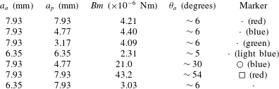
Details of the combinations of sphere–sphere pairs studied in § 4.2. The table includes the following information: the radii of the active spheres $a_{a}$ , the radii of the passive spheres $a_{p}$ , the magnetic torque acting on the active sphere $Bm$ , the approximate amplitude of rotational oscillations of the active sphere $\unicode[STIX]{x1D703}_{a}$ when solitary in the fluid and subject to the applied field, and the corresponding data markers used in figures 7(a,b),8, and 9(a).

The interaction was investigated for various combinations of radii of the active and passive sphere pairs, and for active spheres driven to perform small- and large-amplitude rotary oscillations. A list of the size combinations, the applied magnetic torque and amplitudes of angular oscillation of the active sphere (in the absence of any nearby boundary) is given in table 1.

4 Results

A comparison of the experimental and numerical findings on the interaction between a rotationally oscillating active sphere near a wall, and an active–passive sphere pair are presented in § 4.1 and § 4.2, respectively.

4.1 Angular oscillations of a sphere near a wall

The flow field generated by an oscillating sphere is modified by the presence of a nearby wall. The orientation of the wall relative to the axis of rotation of the sphere has a significant effect on the resulting flow field. Observations show that proximity to the wall results in suppression of the oscillation, at constant magnetic power. These effects are examined for a sphere with an axis of rotation perpendicular and parallel to the wall in § 4.1.1 and § 4.1.2, respectively.

4.1.1 Sphere oscillations about an axis perpendicular to the wall

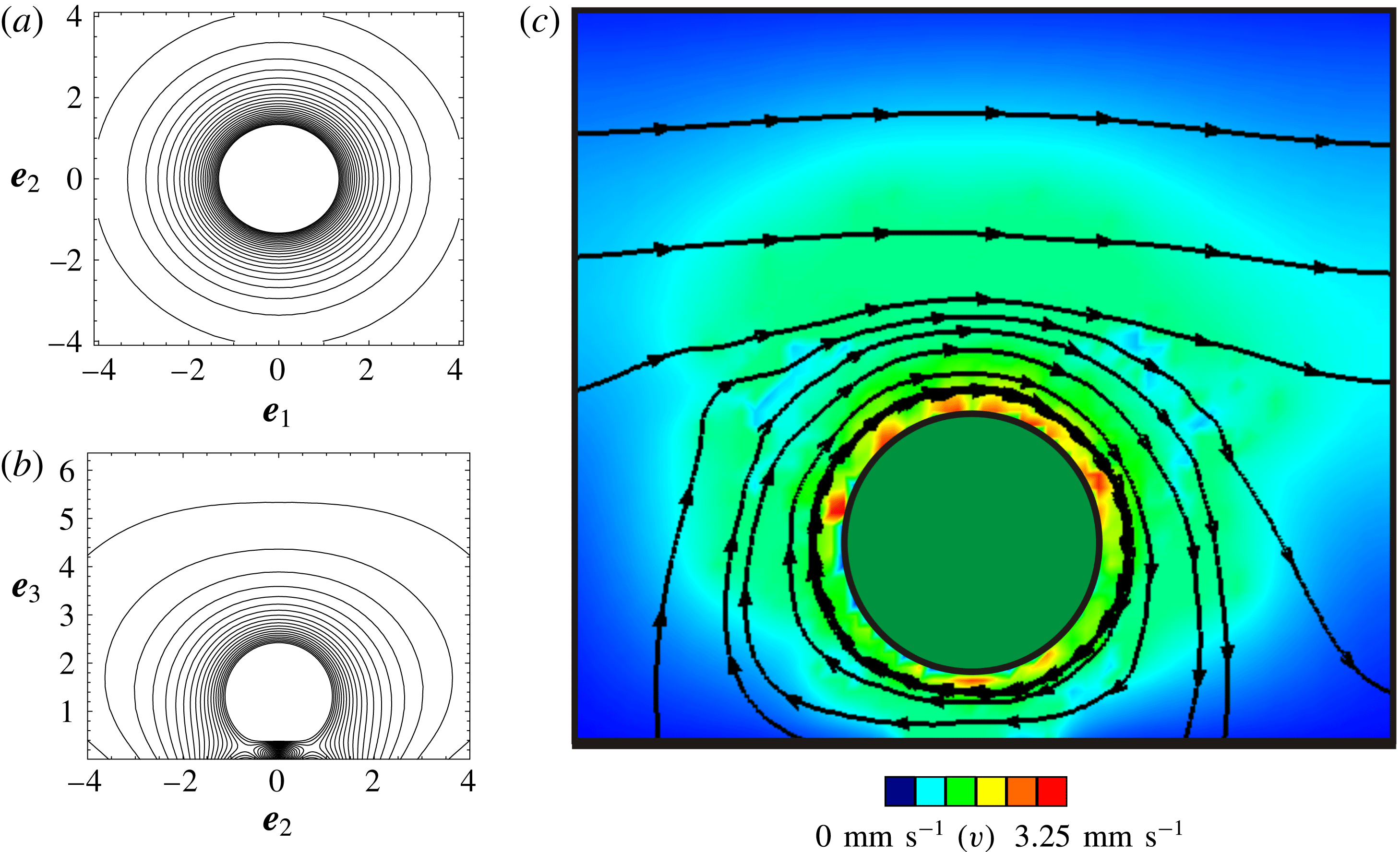
The contour plot of the instantaneous velocity field, shown in figure 3(a), details the characteristic flow around a sphere oscillating about an axis that is perpendicular to a nearby wall at a distance $h/a=1.36$ from the wall (along the $\boldsymbol{e}_{3}$ direction, see caption). In the case of a perpendicular boundary, the flow field in the equatorial plane of the sphere is similar to the unbounded case: the fluid moves in phase with the rotating sphere, with decreasing speed as distance from the boundary of the sphere increases.

Figure 3.

Contour maps of the instantaneous velocity field in the equatorial plane of a rotlet rotating (a) about an axis, $\boldsymbol{e}_{3}$ , that is perpendicular to a wall (i.e. the wall lies parallel to the plane of the page). In (b) the rotlet spins about axis $\boldsymbol{e}_{1}$ , and the wall is perpendicular to the axis of rotation (i.e. the wall is perpendicular to the page intersecting at the abscissa). For both cases, the rotlet is a distance $h/a=1.36$ from the wall, and for the oscillatory rotlet $\unicode[STIX]{x1D714}=0.15~\text{Hz}$ . (c) The instantaneous flow field, in the equatorial plane, generated by a sphere rotating clockwise, at $3\unicode[STIX]{x03C0}/10~\text{radians}$ in the angular oscillation cycle, about an axis that is parallel to the wall and at a vertical distance $h/a=1.36$ from the planar wall (which is represented by the thick horizontal line at the bottom of the figure). The arrowed lines represent instantaneous particle paths and the colour contours represent the magnitude of the fluid velocity which ranges from $0$ (dark blue) to $3.25~\text{mm}~\text{s}^{-1}$ (dark red). Note that figure 3(c) is the experimental counterpart of figure 3(b).

Figure 4.

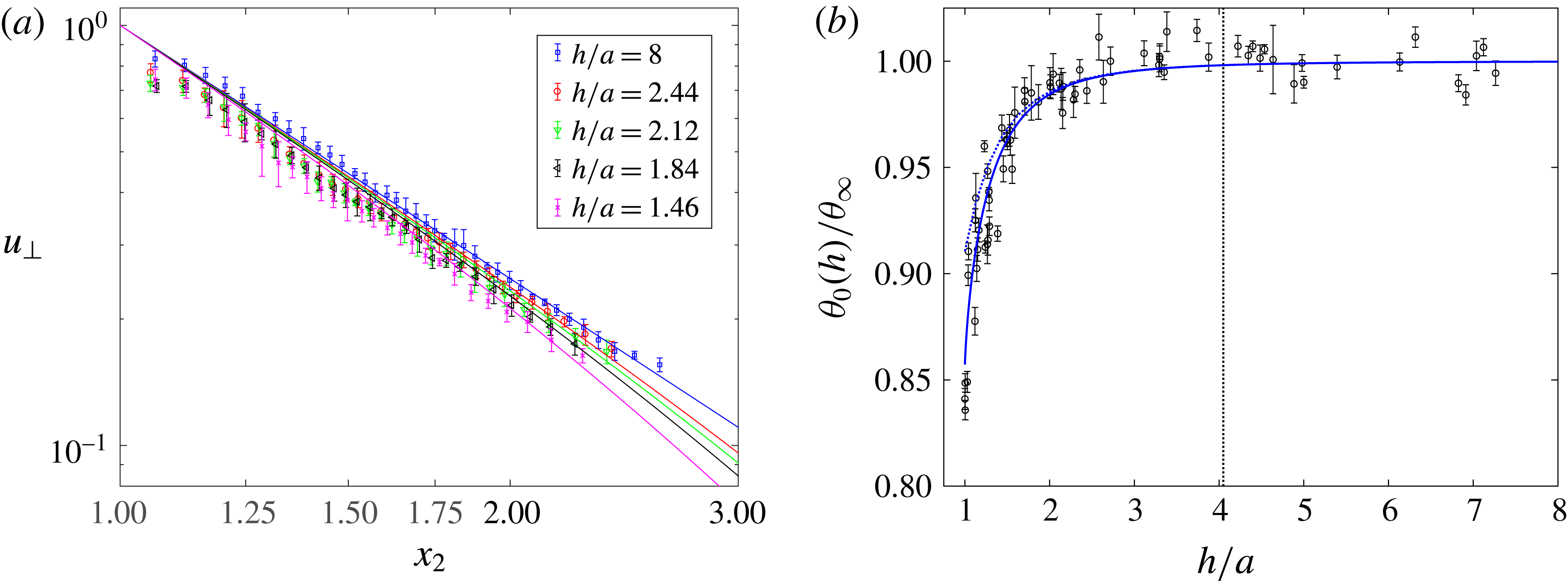
For a sphere oscillating about an axis perpendicular to a wall, the (a) variation of scaled fluid velocity, $u_{\bot }$ , with radial distance from the sphere centre (indicated here by the distance along the $\boldsymbol{e}_{2}$ direction) is plotted for a range of separation distances from the wall, $h$ . Symbols indicate the experimental data (see legend), solid curves of corresponding colour indicate predicted values from (4.1). In (b) the scaled rotational oscillation amplitude, $\unicode[STIX]{x1D703}_{0}(h)/\unicode[STIX]{x1D703}_{\infty }$ , is plotted as a function of separation distance, $h/a$ . The symbols correspond to experimental data (obtained for $\unicode[STIX]{x1D714}=0.5~\text{Hz}$ ) and the dotted curve indicates the predicted value from (2.17) for perpendicular walls, and the solid curves correspond to the multipole method from (A 8). The dashed vertical line denotes the thickness of the Stokes boundary layer from the centre of the sphere, $1+\unicode[STIX]{x1D6FF}/a=4.05$ where $\unicode[STIX]{x1D6FF}=[\unicode[STIX]{x1D708}/(\unicode[STIX]{x03C0}\unicode[STIX]{x1D714})]^{1/2}$ . (Recall that $h/a=1$ corresponds to a sphere touching the wall.)

The suppression of the rotation of the sphere by the wall increases as the distance between the sphere and the wall decreases. In figure 4(a) we compare the amplitude of the predicted and experimental flow velocities over a range of sphere–wall separation distances, $h/a$ . The velocity profile was measured outwards along an axis orthogonal to the axis of rotation from the surface of the sphere and at an angular rotation of $3\unicode[STIX]{x03C0}/10~\text{radians}$ in the oscillation cycle. The symmetry of the flow permitted averaging the velocity profile over the equatorial angle of $2\unicode[STIX]{x03C0}$ , and the averaged profile was found to be consistent to within 1 % throughout the oscillation cycle. In the model we interrogate the flow velocity at a point in the fluid measured in the equatorial plane of the sphere, $\boldsymbol{x}=(0,x_{2},h/a)$ where $x_{2}\in (1,\infty )$ , and estimate the amplitude of the scaled flow velocity:

(4.1)

$$\begin{eqnarray}u_{\bot }(\boldsymbol{x};h)=\frac{|\bar{\boldsymbol{u}}_{\bot }(\boldsymbol{x};h)|}{\unicode[STIX]{x1D703}_{0}(h)},\end{eqnarray}$$

where $\boldsymbol{u}_{\bot }$ and $\unicode[STIX]{x1D703}_{0}(h)$ are defined in (2.11) and (2.17) respectively, and $\bar{\boldsymbol{u}}$ corresponds to the oscillation cycle-averaged velocity, which is equivalently given by the steady rotlet value (as discussed in § 2.2.3).

The fluid velocity decreases with distance from the wall (figure 4 a), and from (2.11), we see that the dipolar $r^{-2}$ decay characteristics prevail at large separation distances from the wall. As the sphere is brought closer to the wall, the small reduction in flow velocity can be explained with the help of the model as being on account of the increased relevance of the counter rotating image rotlet on the sphere. Similarly we see a suppression of the rotational amplitude of the sphere as it approaches the wall, measured as a function of separation distance in figure 4(b). Here the effect of the wall was investigated by measuring the amplitude of rotational oscillations, $\unicode[STIX]{x1D703}_{0}(h)$ at constant magnetic power and varying values of $h$ . We compare the rotlet model prediction with the numerical solution from the multipole method derived by Jeffery (Reference Jeffery1915), and detailed in appendix A, to show the relatively subtle effect of the wall not captured by the simpler rotlet model.

The reduction in the effective amplitude of rotation of the active sphere $\unicode[STIX]{x1D703}_{0}(h)$ is observed for $h/a<1+\unicode[STIX]{x1D6FF}/a\approx 4$ , where the thickness of the Stokes boundary layer, $\unicode[STIX]{x1D6FF}=[\unicode[STIX]{x1D708}/(\unicode[STIX]{x03C0}\unicode[STIX]{x1D714})]^{1/2}$ , gives an estimate of the penetration depth over which the amplitude of fluid motion decays exponentially to $1/e$ of the initial value. In this context we note that Lauga & Powers (Reference Lauga and Powers2009) observed that microorganisms swimming at constant power display characteristics of suppressed swimming speeds near walls, resulting in reduced propulsive efficiency.

4.1.2 Sphere oscillations about an axis parallel to the wall

When the rotational axis of the sphere was set parallel to the nearby wall the flow field was not axisymmetric. We show a contour map of the instantaneous velocity field in the equatorial plane of a rotlet rotating about an axis parallel to the wall, at distance $h/a=1.36$ from the wall, in figure 3(b). This can be compared directly with an example of the instantaneous flow field produced by a sphere and measured using PIV, shown in figure 3(c). Good agreement is found between the predicted velocity field and the experimental particle paths. The findings are also consistent with numerical calculations of stream surfaces generated by a sphere undergoing steady rotation in the proximity of a planar, perpendicular boundary (cf. figure 11a of Liu & Prosperetti (Reference Liu and Prosperetti2010)).

The flow trajectories indicate that in addition to shear exerted by the rotating sphere on the fluid, the fluid is also squeezed into the gap between the sphere and the wall. This leads to stagnation points which form in the gap between the sphere and the wall on either side of the axis of rotation, as can be seen in figure 3(b). The stagnation points are more difficult to discern in the experimental data; the instantaneous nature of the experimental measurements means the near-surface flow measurements are accompanied by small amounts of noise.

Figure 5.

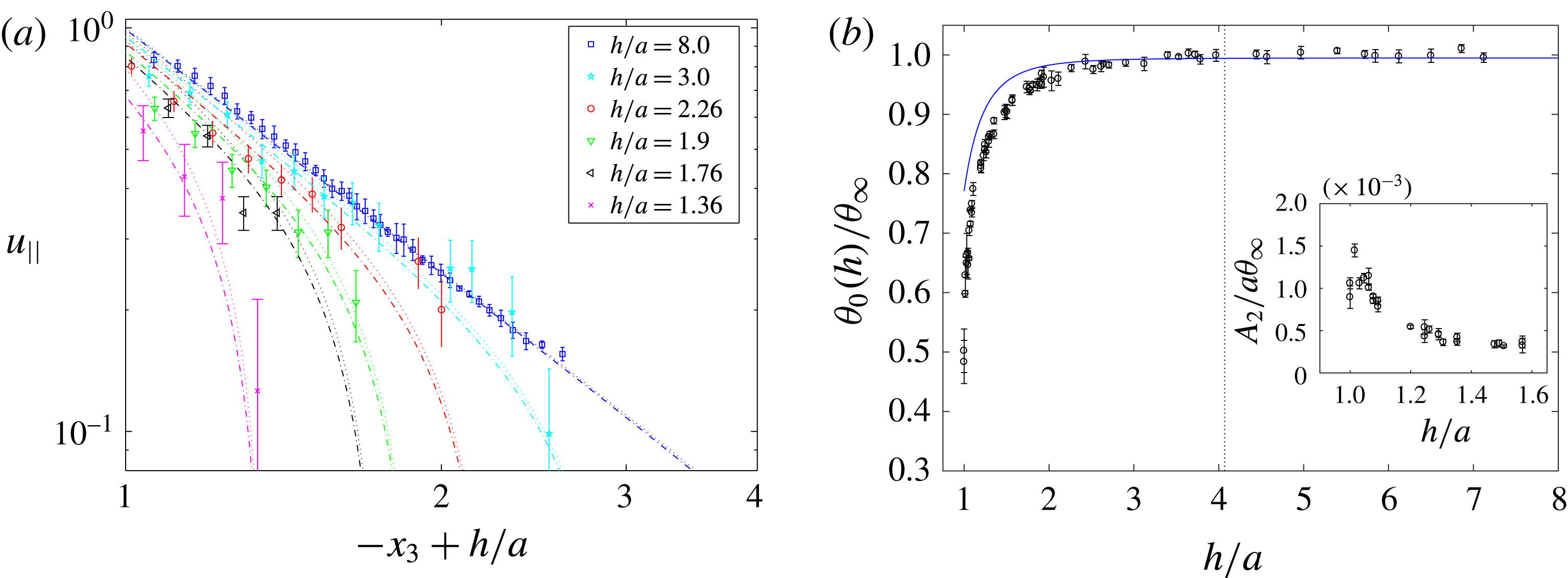
For a sphere oscillating about an axis parallel to a wall, the (a) variation of scaled fluid velocity, $u_{||}$ , is measured in the gap between sphere and wall and for a range of separation distances from the wall, $h$ . Symbols indicate the experimental data (see legend), dotted curves of corresponding colours indicate predicted values from (4.2) and the dash-dotted curves correspond to the case incorporating the rotational angle from the lubrication model. In (b) the scaled amplitude of torsional oscillation, $\unicode[STIX]{x1D703}_{0}(h)/\unicode[STIX]{x1D703}_{\infty }$ , is plotted as a function of separation distance, $h/a$ . The symbols correspond to collated experimental data (obtained for $\unicode[STIX]{x1D714}=0.5~\text{Hz}$ ), the dotted curve indicates the predicted value from (2.17) for parallel walls and the dash-dotted curves are the prediction from the lubrication model in (2.18). The dashed vertical line denotes the thickness of the Stokes boundary layer from the centre of the sphere, $1+\unicode[STIX]{x1D6FF}/a=4.07$ . In the inset figure we plot the scaled translational amplitude of the centre of mass of the sphere, $A_{2}/a\unicode[STIX]{x1D703}_{\infty }$ , with separation distance. (Recall that $h/a=1$ corresponds to a sphere touching the wall.)

The velocity profile in the gap between the sphere surface and the wall was measured. In figure 5(a), we show the amplitude of the experimental flow velocities, scaled by the speed of rotation of the sphere, at various close-range separation distances, $h/a$ , and compare them with the effective large separation case where the container walls are $h/a\sim 8$ from the centre of the sphere. Also shown in figure 5(a) are the theoretical predictions for the scaled velocity amplitude, given by:

(4.2)

$$\begin{eqnarray}u_{||}(\boldsymbol{x};h)=\frac{|\bar{\boldsymbol{u}}_{||}(\boldsymbol{x};h)|}{\unicode[STIX]{x1D703}_{0}(h)},\end{eqnarray}$$

where $\boldsymbol{u}_{||}$ is given by (2.12), $\unicode[STIX]{x1D703}_{0}$ is defined in (2.17), the operator $(\bar{.})$ is as defined for (4.1) and $\unicode[STIX]{x1D703}_{0,L}(h)$ results from the effects of lubrication and is given by (2.18). The theoretical predictions were derived by measuring the flow velocity at a point $\boldsymbol{x}=(0,0,x_{3})$ in the fluid, where $x_{3}\in (h/a-1,1)$ corresponds to a path from sphere boundary to the wall.

The velocity decays with distance from the sphere, however in marked contrast to the case of a perpendicular wall the flow velocity decays significantly as the proximity between the sphere and the wall decreases. Estimation of the near-wall characteristics shows a decay that varies as the cube of the distance from the sphere. Furthermore, as the centre of the sphere was moved closer to the wall, the flow velocity characteristics change from dipolar to quadrupolar.

In figure 5(b) we show the amplitude of the torsional oscillation of the sphere, $\unicode[STIX]{x1D703}_{0}$ , measured as a function of separation distance, $h$ , between the sphere and the wall. Akin to the perpendicular wall case, within the Stokes layer for which $h/a<1+\unicode[STIX]{x1D6FF}/a\approx 4$ , we find that $\unicode[STIX]{x1D703}_{0}(h)$ reduces as the sphere–wall gap is reduced (or as $h/a\rightarrow 1$ ). Although for the parallel-wall case, the amplitude suppression is markedly greater. Lubrication effects dominate very close to the wall and outside this region (for $h/a>1$ ) the rotlet model predicts the fluid velocity more accurately. In the far field both models approach the isolated sphere prediction. In general we see good agreement between the experimental measurements and the model, indicating that the linearised flow assumption is valid almost everywhere except very close to the wall where lubrication effects must be considered.

For $h/a\lesssim 1.5$ viscous shear induced by the parallel wall produces a force which results in secondary translational motion of the sphere along the $\boldsymbol{e}_{2}$ direction. This is consistent with the numerical results of Liu & Prosperetti (Reference Liu and Prosperetti2010), who investigate a sphere undergoing steady rotation in a viscous fluid. Here, the induced translational oscillation of the sphere is sinusoidal in form and in phase with the torsional oscillations of the sphere. The amplitude of translational oscillation of the sphere, $A_{2}(h)$ , moving along $\boldsymbol{e}_{2}$ is shown in the inset to figure 5(b). The amplitude, $A_{2}$ , increases as the sphere approaches the boundary suggesting that the force parallel to the wall increases with viscous shear. As $h/a\rightarrow 1$ , the amplitude of translational oscillation was approximately $40~\unicode[STIX]{x03BC}\text{m}$ , which corresponds to half the arc length subtended by the sphere in one rotary oscillation cycle. However for $h/a\approx 1$ , the amplitude of oscillation reduced to $25~\unicode[STIX]{x03BC}\text{m}$ because of extra frictional effects from roughness.

Finally, we note that these contrasting responses for spheres rotating near perpendicular and parallel boundaries have analogies in translational motion, as observed from studies of micro-organisms swimming near solid walls. The flow field follows dipolar characteristics in the far field, and has a quadrupolar character near a parallel wall (Lauga & Powers Reference Lauga and Powers2009).

4.2 Interaction of sphere–sphere pairs

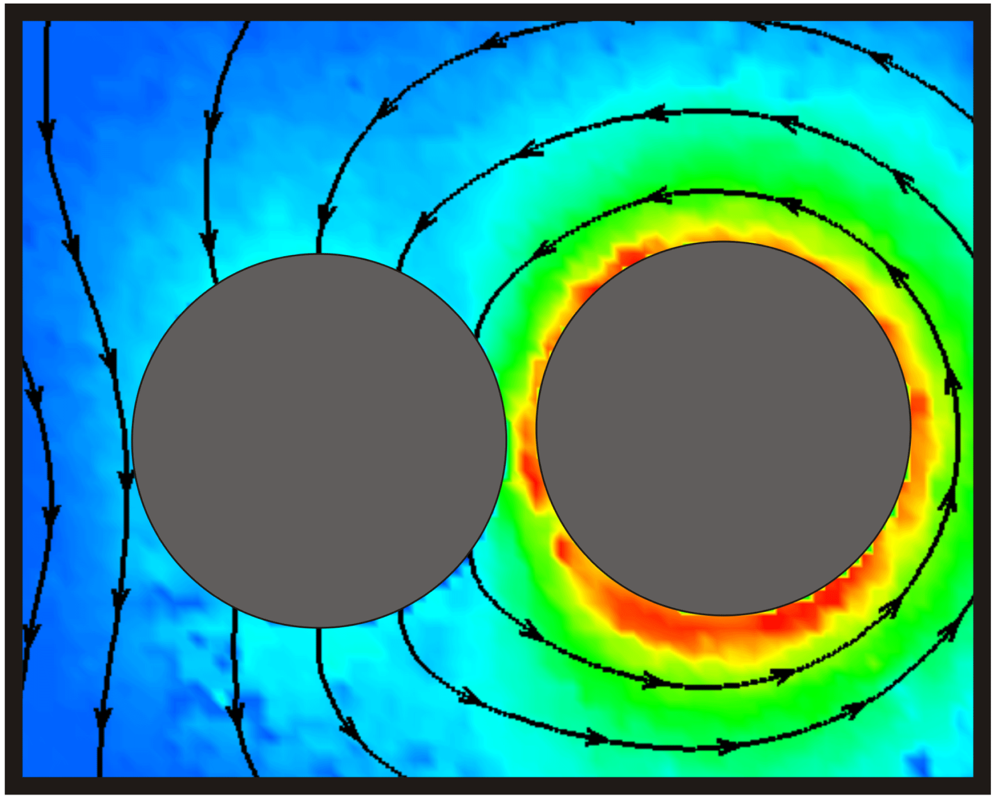
Here we consider the viscous interaction between a rotationally oscillating sphere and a second sphere that is free to move and in the near vicinity. The presence of a second sphere modifies the generated flow field from that of a single rotating sphere, as shown in figure 6. The oscillatory motion of the active sphere induces translational and rotational oscillations in the nearby passive sphere. The motion of the passive sphere further perturbs the flow around the pair, which feeds back to induce translational motion in the active sphere. This induced motion in the active sphere is the principal distinguishing feature with the rigid wall case discussed in § 4.1.2. The schematic diagram in figure 2, illustrates the pair of spheres, and the coupled translational oscillations in the $(\boldsymbol{e}_{2}-\boldsymbol{e}_{3})$ plane, where the active sphere rotates about $\boldsymbol{e}_{1}$ .

Figure 6.

The instantaneous flow field resulting from the interaction between an active sphere (on the right-hand side) and a passive sphere, that is free to move, of equal radius ( $2a=15.86~\text{mm}$ ) at ${\sim}10\unicode[STIX]{x03C0}/6$ in the torsional oscillation cycle, measured in the equatorial plane using the PIV technique. The separation distance, $h$ , between the centres of the two spheres is $2.25a$ . The particle paths are depicted by the black, arrowed lines and the magnitude of the fluid velocity by the colour contours (where blue $=0~\text{mm}~\text{s}^{-1}$ and red $=9.98~\text{mm}~\text{s}^{-1}$ ).

Results are presented for the interactions of spheres of varying radii, and for driven spheres performing small- and large-amplitude angular oscillations (as indicated in table 1). Observations are qualitatively similar for all of the investigated combinations of particle pairs regardless of the radii of active and passive spheres, and whether the active sphere was driven to perform oscillations of small ( $\unicode[STIX]{x1D703}_{a}\sim 6^{\circ }$ ) or large ( $\unicode[STIX]{x1D703}_{a}\sim 50^{\circ }$ ) amplitude. The typical behaviour observed for all separation distances between spheres is discussed in § 4.2.1, whereas the behaviour characteristic to small separation distances is described in § 4.2.2.

4.2.1 Primary effects

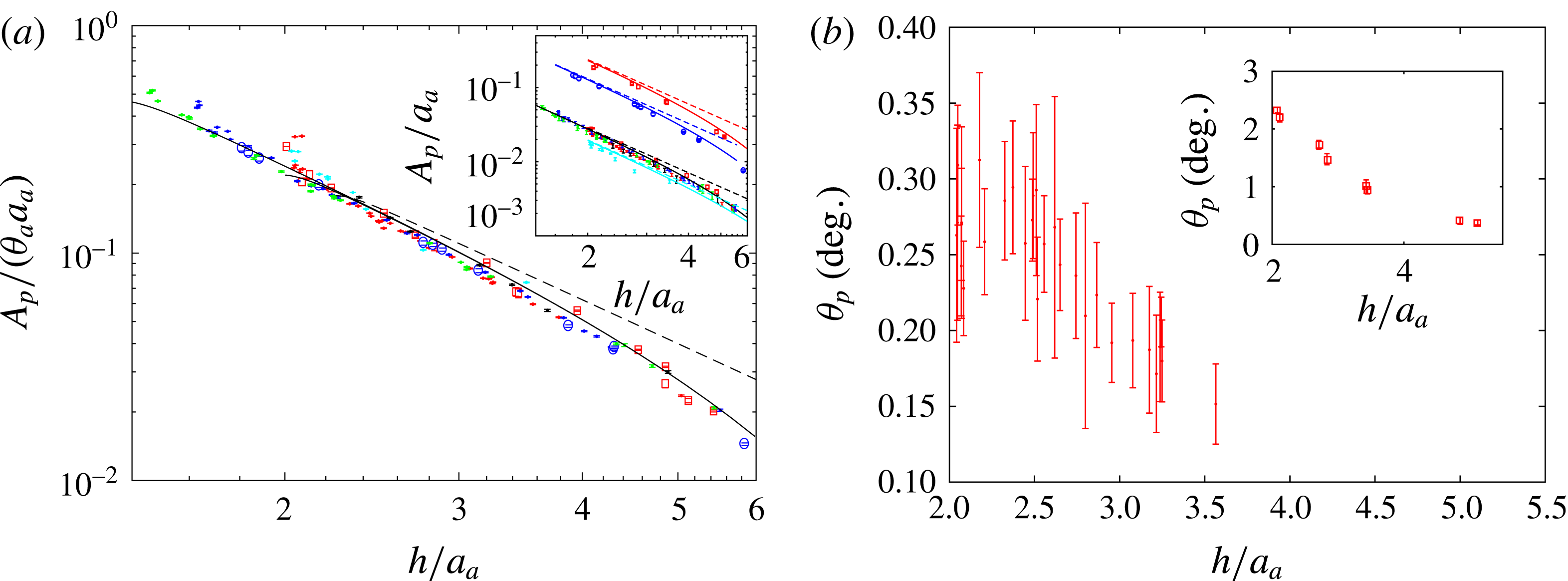
The rotary motion of an active sphere in a viscous fluid perturbs the flow field sufficiently to induce the passive sphere to undergo translational oscillations along $\boldsymbol{e}_{2}$ . The reduction in amplitude of translational motion of the passive sphere, $A_{p}$ , with increasing distance between spheres, $h$ is shown in figure 7(a). When the amplitude of oscillation, $A_{p}$ , is scaled by the arc length subtended by the oscillating active sphere, $a_{a}\unicode[STIX]{x1D703}_{a}$ , the data collapse onto a single curve. Since this result applies for a combination of sphere radii and amplitudes of oscillation, the resulting flow field is similar for a range of pairwise interactions. This scaling also accounts for the suppression of $\unicode[STIX]{x1D703}_{a}$ observed at small separation distances, and is examined further in § 4.2.2.

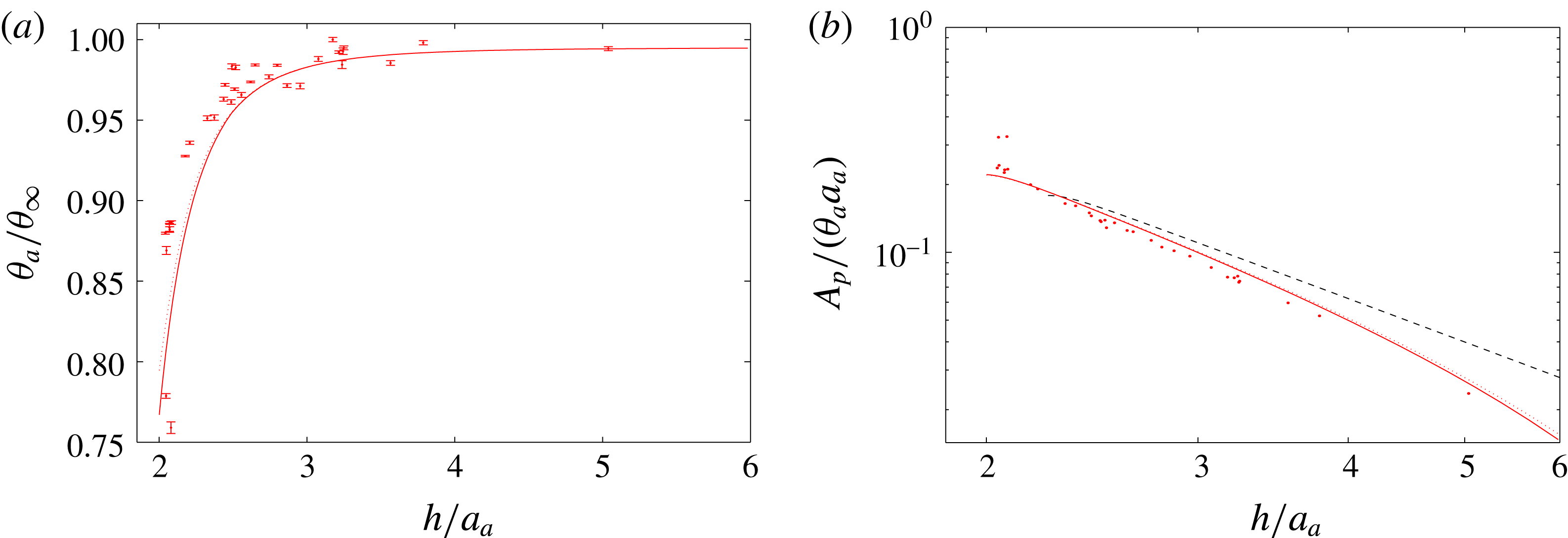
Comparisons between the steady and the quasi-steady oscillating rotlet models, show that for small separation distances ( ${<}2a_{a}$ ), the interaction is effectively modelled by a steady spinning rotlet. However as separation distance between spheres increases the time-varying contribution become increasingly relevant, and the quasi-steady model predicts the measured response well. Note that the lubrication model has been incorporated for sphere pairs, but when compared with the quasi-steady rotlet model the contribution from lubrication to the amplitude of the response of the passive sphere is weak for the case of sphere pairs (for a comparison see figure 11).

Figure 7.

(a) Translational motion of the passive sphere as a function of separation distance, scaled by the characteristic amplitude of the rotational oscillation of the active sphere $a_{a}\unicode[STIX]{x1D703}_{a}$ . The symbols indicate experiments (see table 1), the solid curve indicates predictions from the quasi-steady model and the dashed curve corresponds to the steady solution. The large- and small-amplitude cases may be distinguished from the unscaled data in the inset figure (the data denoted by ○ (blue) and ▫ (red) correspond to oscillations of amplitude ${\sim}30^{\circ }$ and ${\sim}54^{\circ }$ respectively). (b) The amplitude of the rotational oscillation of the passive sphere measured as a function of separation distance from an active sphere of equal radius, $a_{a}=a_{p}$ , performing small-amplitude torsional oscillations, $\unicode[STIX]{x1D703}_{a}\sim 6^{\circ }$ , and (inset) large-amplitude torsional oscillations, $\unicode[STIX]{x1D703}_{a}\sim 54^{\circ }$ .

Figure 8.

The phase difference between the rotational oscillations of the active sphere and the resulting oscillatory motion induced in the passive sphere, $\unicode[STIX]{x1D719}$ , scaled by $\unicode[STIX]{x1D6FF}/a_{a}$ , is plotted as a function of separation distance. The experimentally measured phase difference (see symbols in table 1 for parameter combinations) collapses onto the curve predicted by the model (solid black line) derived in (4.3).

A key feature of the flow is the phase lag between the oscillation cycle in the two spheres. From (2.5) we see that the flow field surrounding the oscillating rotlet decays exponentially with radial distance from the sphere because of viscous diffusion (Stuart Reference Stuart and Rosenhead1963). The imaginary term in (2.7) gives the phase difference (scaled by $(2\unicode[STIX]{x03C0})^{1/2}$ ),

(4.3)

$$\begin{eqnarray}\unicode[STIX]{x1D719}=\frac{[2\unicode[STIX]{x03C0}\unicode[STIX]{x1D6FC}]^{1/2}r}{2}=\frac{a_{a}r}{[2\unicode[STIX]{x1D708}/(\unicode[STIX]{x03C0}\unicode[STIX]{x1D714})]^{1/2}},\end{eqnarray}$$

between fluid particles distance $r$ from the sphere. The phase difference arises from vorticity that is generated by a standing wave in the fluid by the oscillating sphere and propagates within the Stokes layer. The standing wave is established by the rotary oscillations of the active sphere in a manner analogous to the classic case of an oscillating plate in a viscous fluid. The resultant phase difference scales linearly with distance from the sphere, $a_{a}r$ and inversely with the Stokes layer thickness, $\unicode[STIX]{x1D6FF}=[\unicode[STIX]{x1D708}/(\unicode[STIX]{x03C0}\unicode[STIX]{x1D714})]^{1/2}$ .

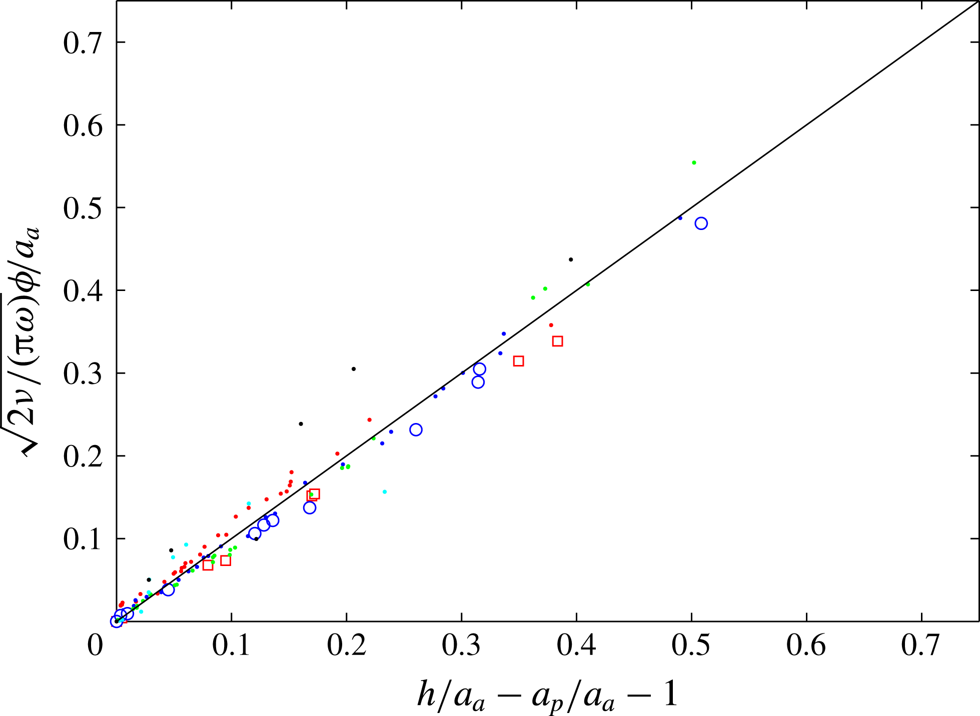
In figure 8, we plot the scaled phase difference between the rotary oscillations of the active sphere and the translational oscillation of the passive sphere, $\sqrt{2\unicode[STIX]{x1D708}/(\unicode[STIX]{x03C0}\unicode[STIX]{x1D714})}\unicode[STIX]{x1D719}/a_{a}$ , measured as a function of the inter-sphere wall distance, $(h/a_{a}-a_{p}/a_{a}-1)$ . For the various combinations of sphere pairs listed in table 1, the data collapse onto the theoretical curve, indicating excellent agreement between experiments and the linear model. The experiments were conducted in the range $0.01\lesssim Re\lesssim 0.1$ , hence the contribution of any inertial effects is small. Thus the assumption of quasi-steady Stokes flow is valid, suggesting that the main mechanism of energy transfer from the active sphere to the surrounding fluid is through vorticity.

The vorticity imparted to the surrounding fluid by the standing wave also induces small-amplitude angular oscillations in the passive sphere in the direction opposite to the motion of the active sphere. The amplitude of rotation of the passive sphere, $\unicode[STIX]{x1D703}_{p}$ is found to decrease with inter-sphere separation distance $h$ , as shown in figure 7(b) for $a_{a}=a_{p}$ and $\unicode[STIX]{x1D703}_{a}\sim 6^{\circ }$ and, in the inset to figure 7(b), for $\unicode[STIX]{x1D703}_{a}\sim 54^{\circ }$ .

4.2.2 Effects which occur at small separations

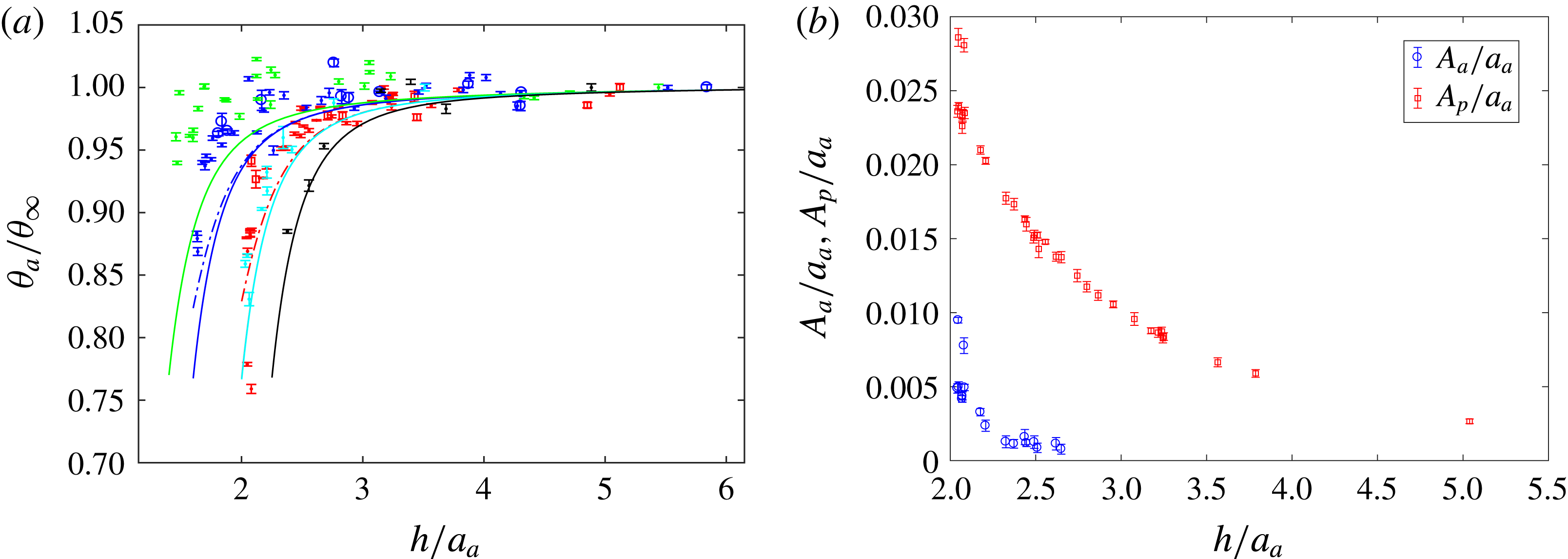
For $h/a_{a}>1+\unicode[STIX]{x1D6FF}/a_{a}\approx 4$ , the presence of the passive sphere does not affect the response of the active sphere to the applied field. However, for $h/a_{a}<4$ , viscous effects reduce the oscillation amplitude of the active sphere. The amplitude of rotational oscillation of the active sphere, $\unicode[STIX]{x1D703}_{a}$ , measured as a function of separation distance, $h$ , is shown in figure 9(a) for various combinations of pairs of spheres. The effect of the passive sphere is to reduce the oscillation amplitude of the active sphere, and this effect becomes stronger as the spheres are brought closer together. The phenomenon is similar to an active sphere oscillating close to a parallel wall, although for sphere pairs the experimental data suggest the amplitude suppression is mitigated, an observation which is attributed to the wall curvature and the resultant motion of the passive sphere itself. Here, as in the case of a parallel wall, we include the effect of lubrication on the angular amplitude response (see (A 6)), based on the expression derived in (A 1).

Figure 9.

(a) Suppression of rotational oscillations of the active sphere given by $\unicode[STIX]{x1D703}_{a}/\unicode[STIX]{x1D703}_{\infty }$ for varying $h$ and the various combination of parameters as indicated in table 1 are compared with the theoretical model which includes the lubrication model (solid curves). The dash-dotted curves correspond to the cases with large-amplitude oscillations (see table 1). (b) The amplitude of translation oscillation of a passive sphere (▫) and an active sphere (○) of equal radii, measured as a function of separation distance for $\unicode[STIX]{x1D703}_{a}\sim 6$ . (Recall that $h/a_{a}=2$ corresponds to two equal-sized spheres touching.)

For very small separation distances, translational oscillations of the passive sphere perturb the flow field sufficiently to induce secondary translational motion in the active sphere, with the oscillations approximately out of phase with each other. In figure 9(b) we compare the primary passive and secondary active sphere amplitudes of translational oscillation, $A_{a}$ and $A_{p}$ respectively. The amplitude decreases with increasing separation distance, $h$ . The secondary oscillations in the active sphere are perceptible for $h/a_{a}<3$ and are a consequence of the generated wall-parallel force. This is akin to the translational displacement of an active sphere observed for small separation distances from a parallel wall examined in § 4.1.2 and figure 5(b). The displacement of the active sphere arises from the fluidic interactions between the pair of mobile spheres. Note that the induced motion in the active sphere has not been modelled in (2.21) and is likely to account for the small differences between experimental results and the model predictions at very small separation.

5 Conclusions

The fluid dynamics of oscillating spheres near boundaries has been studied. A novel experimental approach used magnetic interactions to control the rotational oscillations of a sphere in a viscous fluid without affecting the local fluid environment. This enabled quantitative measurement of the flow field in unprecedented detail. The experimental results have been compared with those from a theoretical model based on singularity methods where it was assumed the motion was quasi-steady Stokes flow near boundaries. Excellent agreement has been found between experimental and theoretical results.

We found that the presence of a nearby rigid boundary introduces a resistive torque that opposes the motion of the driven sphere and the surrounding fluid if the gap between the sphere and the wall is less than the thickness of the Stokes boundary layer. This suppression of rotational motion depends on the orientation of the boundary with respect to the rotation of the sphere; in particular, it is stronger for the case where the wall is aligned parallel to the axis of rotation, as compared to a perpendicular alignment. Our results suggest that, for small-amplitude oscillations near a rigid boundary, there is virtually no difference between the time-averaged or instantaneous velocity of a fluid particle near the sphere such that the sphere motion and fluid response can be considered to be time independent with no loss of generality.

We also found that fluid dynamic interactions can cause a nearby, non-magnetic, passive sphere to move in response to a driven sphere such that it acts like a moving curved wall, oscillating with a phase lag that scales linearly with separation distance between the spheres. The phase lag is a consequence of the oscillatory motion of the driven sphere which establishes a standing wave that imparts vorticity to the surrounding fluid. For small separation distances, $h<2a_{a}$ , the response of the passive sphere to the driven sphere is modelled by considering a steady spinning rotlet. As the inter-sphere distance increases the time-varying contribution to the flow becomes more important, however, and the interaction is better predicted using a quasi-steady model, which highlights the important distinction between interacting sphere pairs with the solitary sphere near a stationary wall. As the gap reduces below one sphere radius, lubrication effects become increasingly important (although weaker than in the case of a stationary, parallel wall) and the motion of the passive sphere induces secondary translation of the driven sphere. These small-amplitude translational oscillations of the active sphere are periodic, reflecting the symmetry and reversibility of the flow, and decay rapidly with increasing separation, consistent with the higher-order effects observed between pairs of swimming cells (Lauga & Powers Reference Lauga and Powers2009).

The findings provide the basis for the development of a magnetically actuated, rotational sphere viscometer for use in medical, biological and micro-fluidic applications. Such a device would be able to measure the rheological properties of fluids (Besseris et al. Reference Besseris, Miller and Yeates1999) in micro-fluidic devices or in between biological tissue. Experiments performed within cells and with vitreous fluid have already demonstrated the suitability of rotating sphere viscometers for non-invasive, in vivo testing (Parkin et al. Reference Parkin, Knoner, Nieminen, Heckenberg and Rubinsztein-Dunlop2007).

Another avenue of research currently being pursued is an investigation into the resulting flow that arises when active and passive spheres are connected together by deformable tethers (Box et al. Reference Box, Han, Tipton and Mullin2017). Arrays of magnetically actuated spheres have been shown to overcome time reciprocity and self-propel at low $Re$ . These systems could therefore be used as micro-fluidic pumping systems, or as configurable micro-fluidic channels for the transportation of micron-scale objects (Ye, Diller & Sitti Reference Ye, Diller and Sitti2012). The numerical scheme presented here provides an efficient means of modelling complex configurations of active and passive spheres accurately.

Acknowledgements

The authors are grateful to Professor Sir K. Novoselov FRS and Professor A. Murray for the loan of equipment, and to the anonymous referees for their helpful comments on an earlier draft of the paper. T.M. would also like to acknowledge the support of a Leverhulme Trust Emeritus Fellowship.

Appendix A

A.1 Rotationally oscillating spheres in near contact with parallel boundaries

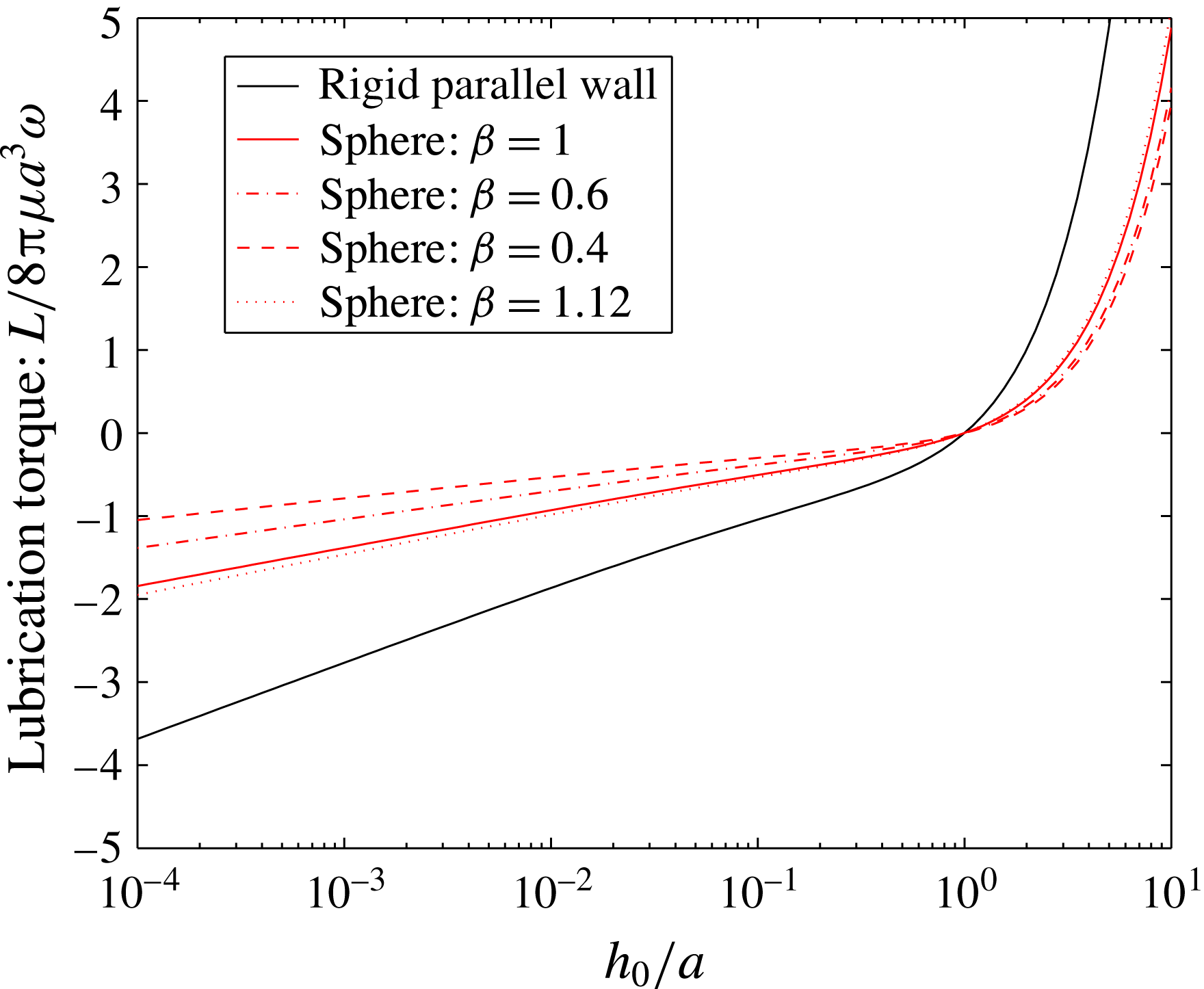
In this section we focus on the specific case of oscillating spheres in very close proximity to rigid boundaries that are orientated parallel to the sphere’s axis of rotation. For rigid surfaces where there is relative motion, the flow of fluid in the gap between the surfaces starts to dominate, and lubrication theory can be used to approximately estimate the contribution of this region (Kim & Karrila Reference Kim and Karrila1991).

The main motivation to model the lubrication regime was the strong suppression in rotation and the marked reduction in flow velocity that were observed experimentally as the sphere approaches the boundary. We now consider the viscous contribution to the torque balance equation (2.1) carefully. Following the analysis of Kim & Karrila (Reference Kim and Karrila1991), we see that a sphere performing rotational oscillations with angular velocity $\unicode[STIX]{x1D714}$ and in close proximity to another sphere, generates a contribution to the viscous torque in the gap between the spheres that, to leading order, is given by:

(A 1)

$$\begin{eqnarray}\frac{{\mathcal{L}}_{s}}{8\unicode[STIX]{x03C0}\unicode[STIX]{x03BC}a_{a}^{3}\unicode[STIX]{x1D714}_{a}}=\frac{2\unicode[STIX]{x1D6FD}}{5(1+\unicode[STIX]{x1D6FD})}\ln \left(\frac{h_{0}}{a_{a}}\right)+\frac{2(8+6\unicode[STIX]{x1D6FD}+33\unicode[STIX]{x1D6FD}^{2})}{125(1+\unicode[STIX]{x1D6FD})^{2}}\left(\frac{h_{0}}{a_{a}}\right)\ln \left(\frac{h_{0}}{a_{a}}\right)+C(\unicode[STIX]{x1D6FD}),\end{eqnarray}$$

where $\unicode[STIX]{x1D6FD}=a_{p}/a_{a}$ and $h_{0}=h-a_{a}(1+1/\unicode[STIX]{x1D6FD})$ (parameters $h,a,a_{a},a_{p},\unicode[STIX]{x1D714}$ are as defined in §§ 2.1, 2.3). Note the special case of equal-sized spheres $(\unicode[STIX]{x1D6FD}=1)$ where (A 1) simplifies to give,

(A 2)

$$\begin{eqnarray}\frac{{\mathcal{L}}_{s,eq}}{8\unicode[STIX]{x03C0}\unicode[STIX]{x03BC}a_{a}^{3}\unicode[STIX]{x1D714}}=\frac{1}{5}\ln \left(\frac{h_{0}}{a_{a}}\right)+\frac{57}{250}\left(\frac{h_{0}}{a_{a}}\right)\ln \left(\frac{h_{0}}{a_{a}}\right)+C.\end{eqnarray}$$

We next use (A 1) and extend it to consider a sphere oscillating about an axis parallel to a rigid wall (setting $1/\unicode[STIX]{x1D6FD}\rightarrow 0$ ):

(A 3)

$$\begin{eqnarray}\frac{{\mathcal{L}}_{w}}{8\unicode[STIX]{x03C0}\unicode[STIX]{x03BC}a^{3}\unicode[STIX]{x1D714}}=\frac{2}{5}\ln \left(\frac{h_{0}}{a}\right)+\frac{66}{125}\left(\frac{h_{0}}{a}\right)\ln \left(\frac{h_{0}}{a}\right)+C,\end{eqnarray}$$

and here $h_{0}=h-a$ . Comparing (A 2) and (A 3) it is easy to see that the dampening effect of a rigid wall is almost twice as strong as for a pair of spheres of equal radius. This observation may be visualised in figure 10 where we plot the contribution of the lubrication layer to the viscous torque for representative cases examined in the experiments (cf. table 1).

Figure 10.

The contribution to the viscous torque by the lubrication layer in the gap between actively rotating sphere and corresponding boundary is indicated here as the lubrication torque ${\mathcal{L}}(h)$ , as given by (A 1), (A 3). The rigid wall case is compared with pairs of spheres of differing radii, where $\unicode[STIX]{x1D6FD}=a_{p}/a_{a}$ ( $C=0$ here).

Figure 11.

(a) Amplitude of rotary oscillation of the active sphere scaled by the amplitude of oscillation in the absence of a nearby boundary and measured as a function of separation distance for the case of an equal radius passive–active pair $(a_{p}=a_{a}=7.83~\text{mm})$ ; comparing the unsteady rotlet model with (solid curves) and without (dotted curves) lubrication effects. The experimental data shown ( $\cdot$ (red) symbols) correspond to the small-amplitude case ( ${\sim}6^{\circ }$ ). (b) Amplitude of translational motion of the passive sphere, scaled by the arc length subtended by the active sphere and measured as a function of separation distance for the same case as in (a) (also same symbols and curves). Here we also plot the steady spinning rotlet model (dashed curve).

We next account for the contribution of the lubrication layer in suppressing the sphere response to an external magnetic torque. Including the contribution of lubrication, the net viscous torque can be expressed as

(A 4)

$$\begin{eqnarray}T_{v}=8\unicode[STIX]{x03C0}\unicode[STIX]{x03BC}a^{3}\unicode[STIX]{x1D714}(1+{\mathcal{L}}(h)),\end{eqnarray}$$

where ${\mathcal{L}}(h)$ is given by (A 1) and (A 3) respectively, depending upon whether the boundary is a sphere or parallel wall.

The magnetic torque is unchanged so $T_{m}=B_{0}m\sin \check{\unicode[STIX]{x1D703}}\text{e}^{\text{i}\unicode[STIX]{x1D714}t}$ , and the torque balance equation becomes:

(A 5)

$$\begin{eqnarray}\frac{\text{d}\unicode[STIX]{x1D703}}{\text{d}t}=-\frac{B_{0}m}{8\unicode[STIX]{x03C0}\unicode[STIX]{x03BC}a^{3}(1+{\mathcal{L}}(h))}\sin (\check{\unicode[STIX]{x1D703}}(t))\text{e}^{\text{i}\unicode[STIX]{x1D714}t}.\end{eqnarray}$$

However, in the lubrication layer the assumption that $\unicode[STIX]{x1D703}(t)\ll \bar{\unicode[STIX]{x1D703}}$ is no longer valid, although the pronounced reduction in amplitude requires that $\check{\unicode[STIX]{x1D703}}\ll 1$ . Therefore we can now assume $\sin \check{\unicode[STIX]{x1D703}}\approx \bar{\unicode[STIX]{x1D703}}+\unicode[STIX]{x1D703}(t)$ , and by integrating over an oscillation cycle the expression for the amplitude of oscillation is given as:

(A 6)

$$\begin{eqnarray}\unicode[STIX]{x1D703}_{0,L}(h)=C_{1}\exp \left(-\frac{C_{0}}{M_{a}(1+{\mathcal{L}}(h))}\right),\end{eqnarray}$$

where $M_{a}$ is the Mason number defined in § 2.1 and $C_{0}$ includes the phase difference between the alternating field and the sphere’s response, $C_{1}$ is a constant; both $C_{1}$ and $C_{2}$ depend on the initial configuration and are estimated empirically. Note that in the limiting case of an isolated sphere where ${\mathcal{L}}=0$ , $\unicode[STIX]{x1D703}_{\infty }=C\exp (-C_{\infty }/M_{a})$ , and we can express $\unicode[STIX]{x1D703}_{0,L}(h)=\unicode[STIX]{x1D703}_{\infty }\exp (-(1/M_{a})[C_{0}/(1+{\mathcal{L}}(h))-C_{\infty }])$ .

In figure 11(a) we compare predictions for a pair of equally sized spheres ( $\unicode[STIX]{x1D6FD}=1$ ) using the unsteady model developed in § 2.3 and the correction to the angular amplitude due to lubrication effects as given by (A 6). Our observation that the impact of the lubrication layer on the suppression of motion of the active sphere is much lower in the case of a sphere pair than for the rigid wall is borne out in these results (also see the rigid wall predictions in figure 5). Similarly the response of passive sphere has been compared in figure 11(b). Interestingly, we find that small discrepancies between model predictions and experiments that occur very near the wall (see figure 11 b) are not a consequence of lubrication effects. We instead believe that these discrepancies are either an artefact of the secondary translational oscillations of the active sphere that are induced by the motion of the passive sphere, and are not currently included in the model, or are a consequence of intermittent contact between the spheres.

Finally, it is worth noting that the unsteady rotlet model retrieves the experimental response with a high degree of accuracy, and including lubrication effects is to improves the accord with experiments.

A.2 Rotationally oscillating spheres in near contact with perpendicular boundaries

The case of a spinning sphere about an axis perpendicular to a wall has been examined by Jeffery (Reference Jeffery1915). Multipole methods were used to obtain solutions to the mobility and resistance problems. We use this method to evaluate the error in the simpler, more approximate rotlet model developed in § 2.2.1. Following Jeffery (Reference Jeffery1915), we show that the torque acting on a sphere spinning about an axis perpendicular to a rigid wall is given as

(A 7)

$$\begin{eqnarray}\frac{T_{\bot }^{v}}{T_{\infty }}=\left[1-\frac{\displaystyle \mathop{\sum }_{m=0}^{\infty }\text{cosech}^{3}[2(m+1)\unicode[STIX]{x1D701}]}{\displaystyle \mathop{\sum }_{m=0}^{\infty }\text{cosech}^{3}[(2m+1)\unicode[STIX]{x1D701}]}\right]^{-1},\end{eqnarray}$$

where $T_{\infty }$ is the far-field torque. Also $\unicode[STIX]{x1D701}=\text{sech}^{-1}(1/h)$ , $h$ is the separation distance of the sphere centre from the wall scaled by sphere radius $a$ (and as defined in § 2). We plot this curve in figure 12.

Using $\boldsymbol{T}_{\bot }^{v}=8\unicode[STIX]{x03C0}\unicode[STIX]{x03BC}a^{3}\unicode[STIX]{x1D714}_{1}$ , $\unicode[STIX]{x1D714}_{1}=\text{d}\unicode[STIX]{x1D703}/\text{d}t,\unicode[STIX]{x1D703}(h;t)=\unicode[STIX]{x1D703}_{0}(h)\exp (\text{i}\unicode[STIX]{x1D714}t)$ . Since $\unicode[STIX]{x1D703}\ll \bar{\unicode[STIX]{x1D703}}$ the amplitude of angular oscillation, for the case of a perpendicular-wall case relative to the far-field angular amplitude is

(A 8)

$$\begin{eqnarray}\frac{\unicode[STIX]{x1D703}_{0}(h)}{\unicode[STIX]{x1D703}_{\infty }}=\frac{T_{\infty }}{T_{\bot }^{v}}.\end{eqnarray}$$

Figure 12.

The increase in viscous torque due to the near-wall relative to the far-field response for a perpendicular wall.

References

Ambari, A., Gauthier-Manuel, B. & Guyon, E. 1984 Wall effects on a sphere translating at constant velocity. J. Fluid Mech. 149, 235–253.Google Scholar

Ardekani, A. & Rangel, R. 2006 Unsteady motion of two solid spheres in Stokes flow. Phys. Fluids 18, 103306.Google Scholar

Besseris, G., Miller, I. F. & Yeates, D. B. 1999 Rotational magnetic particle microrheometry: the Newtonian case. J. Rheol. 43, 591–608.Google Scholar

Blake, J. R. & Chwang, A. T. 1974 Fundamental singularities of viscous flow. J. Engng Maths 8, 23–29.Google Scholar

Box, F., Han, E., Tipton, C. R. & Mullin, T. 2017 On the motion of linked spheres in a Stokes flow. Exp. Fluids 58, 29.Google Scholar

Box, F., Thompson, A. B. & Mullin, T. 2015 Torsional oscillations of a sphere in a Stokes flow. Exp. Fluids 56, 209.Google Scholar

Buchanan, J. 1891 The oscillations of a spheroid in a viscous liquid. Proc. Lond. Math. Soc. 22, 181–214.Google Scholar

Cichocki, B., Felderhof, B. U., Hinsen, K., Wajnryb, E. & Blawzdziewicz, J. 1994 Friction and mobility of many spheres in a Stokes flow. J. Chem. Phys. 100, 3780–3790.Google Scholar

Cichocki, B., Felderhof, B. U. & Schmitz, R. 1988 Hydrodynamic interactions between two spherical particles. Physico-Chem. Hydrodyn. 10, 383–403.Google Scholar

Cox, R. G. & Brenner, H. 1967 The slow motion of a sphere through a viscous fluid towards a plane surface. II. Small gap widths, including inertial effects. Chem. Engng Sci. 22, 1753–1777.Google Scholar

Crocker, J. C. 1997 Measurement of the hydrodynamic correction to the Brownian motion of two colloidal spheres. J. Chem. Phys. 106, 2837–2840.Google Scholar

Dean, W. R. & O’Neill, M. E. 1963 A slow motion of viscous liquid caused by the rotation of a solid sphere. Mathematika 10, 13–24.Google Scholar

Faxén, H. 1922 The resistance against the movement of a rigour sphere in viscous fluids, which is embedded between two parallel layered barriers. Ann. Phys. 68, 89–119.Google Scholar

Goldman, A. J., Cox, R. G. & Brenner, H. 1967 Slow viscous motion of a sphere parallel to a plane wall. I. Motion through a quiescent fluid. Chem. Engng Sci. 22, 637–651.Google Scholar

Guazzelli, E. & Hinch, J. 2010 Fluctuations and instability in sedimentation. Annu. Rev. Fluid Mech. 43, 97–116.Google Scholar

Happel, J. & Brenner, H. 1983 Low Reynolds Number Hydrodynamics with Special Applications to Particulate Media, 1st edn. Springer.Google Scholar

Henderson, S. I., Mitchell, S. J. & Bartlett, P. 2001 Direct measurements of colloidal friction coefficients. Phys. Rev. E 64, 061403.Google Scholar

Henderson, S. I., Mitchell, S. J. & Bartlett, P. 2002 Propagation of hydrodynamic interactions in colloidal suspensions. Phys. Rev. Lett. 88, 088302.Google Scholar

Jeffery, G. B. 1915 On the steady rotation of a solid of revolution in a viscous fluid. Proc. Lond. Math. Soc. 14, 327338.Google Scholar

Jeffrey, D. J. 1992 The calculation of the low Reynolds-number resistance functions for two unequal spheres. Phys. Fluids 4, 16–29.Google Scholar

Jeffrey, D. J. & Onishi, Y. 1984a Calculation of the resistance and mobility functions for two unequal rigid spheres in low-Reynolds number flow. J. Fluid Mech. 139, 261–290.Google Scholar

Jeffrey, D. J. & Onishi, Y. 1984b The forces and couples acting on two nearly touching spheres in low-Reynolds number flow. Z. Angew. Math. Phys. 35, 634–641.Google Scholar

Kestin, J. & Persen, L. N.1954 Small oscillations of bodies of revolution in a viscous fluid. Brown University Report AF-891/2, Contract A718(600)-891.Google Scholar

Kim, I. & Miffin, R. T. 1985 The resistance and mobility functions of two equal spheres in low-Reynolds-number flow. Phys. Fluids 28, 2033–2045.Google Scholar

Kim, S. & Karrila, S. J. 1991 Microhydrodynamics: Principles and Selected Applications, 1st edn. Butterworth-Heinemann.Google Scholar

Kim, S. & Russel, W. 1985 Modelling of porous media by renormalization of the Stokes equations. J. Fluid Mech. 154, 269–286.Google Scholar

Lamb, H. 1932 Hydrodynamics, 6th edn. Dover.Google Scholar

Lauga, E. & Powers, T. R. 2009 The hydrodynamics of swimming microorganisms. Rep. Prog. Phys. 72, 096601.Google Scholar

Liu, Q. & Prosperetti, A. 2010 Wall effects on a rotating sphere. J. Fluid Mech. 657, 1–21.Google Scholar

Meiners, J. C. & Quake, S. R. 1999 Direct measurement of the hydrodynamic cross-correlations between two particles in an external potential. Phys. Rev. Lett. 82, 2211–2214.Google Scholar

Parkin, S. J., Knoner, G., Nieminen, T. A., Heckenberg, N. R. & Rubinsztein-Dunlop, H. 2007 Picoliter viscometry using optically rotated particles. Phys. Rev. E 76, 041507.Google Scholar

Pozrikidis, C. 1989 A singularity method for unsteady linearized flow. Phys. Fluids 1, 1508.Google Scholar

Steinbach, G., Gemmin, S. & Erbe, A. 2016 Rotational friction of dipolar colloids measured by driven torsional oscillations. Sci. Rep. 6, 34193.Google Scholar

Stimson, M. & Jeffrey, G. B. 1926 The motion of two spheres in a viscous fluid. Proc. R. Soc. Lond. A 111, 110–116.Google Scholar

Stuart, J. T. 1963 Unsteady boundary layers. In Laminar Boundary Layers (ed. Rosenhead, L.), pp. 349–408. Oxford University Press.Google Scholar

Trankle, B., Speidel, M. & Rohrbach, A. 2012 Interaction dynamics of two colloids in a single optical potential. Phys. Rev. E 86, 021401.Google Scholar

Ye, Z., Diller, E. & Sitti, M. 2012 Micro-manipulation using rotational fluid flows induced by remote magnetic micro-manipulators. J. Appl. Phys. 112, 064912.Google Scholar

Figure 1.(a,b) Schematic diagrams of a sphere of radius $a$ undergoing rotational oscillations about axes (a) $\boldsymbol{e}_{3}$ (perpendicular to the wall) and (b) $\boldsymbol{e}_{1}$ (parallel to the wall), respectively. The axis of rotation is indicated by the dotted, curved arrow. The applied external magnetic field vector lies along $\pm \boldsymbol{e}_{1}$ and $\pm \boldsymbol{e}_{2}$ in (a) and (b) respectively, the embedded magnets are depicted in grey, the dipole axis is the grey dashed line, the baseline dipole angle is $\bar{\unicode[STIX]{x1D703}}$ and the angular oscillation contribution is $\unicode[STIX]{x1D703}(t)$. The spheres are distance $h$ from the wall, where the wall normal is along $\boldsymbol{e}_{3}$. (c,d) Schematic diagrams illustrating the model for a rotating sphere, represented by a rotlet singularity, and the corresponding image system for a wall where the axis of rotation of the sphere lies (c) along $\boldsymbol{e}_{3}$, perpendicular to, and (d) $\boldsymbol{e}_{1}$, parallel to, the wall (Blake & Chwang 1974).

Figure 2.Schematic diagrams of the sphere pair, comprising an active sphere (radius $a_{a}$, centre at $o_{a}$) and passive sphere (radius $a_{p}$, centre at $o_{p}$) with the sphere centres $o_{a},o_{p}$ distance $h$ apart. The diagrams show the (a) initial undisturbed state and (b) instantaneous perturbed state when magnetically activated with active sphere centre to passive sphere wall distance $h^{\prime }(t)=h-a_{p}\cos \unicode[STIX]{x1D6FE}(t)$. The active sphere rotates through angle $\unicode[STIX]{x1D703}_{a}$ about axis $\boldsymbol{e}_{3}$, perturbing the surrounding fluid. The configuration results in induced rotation $\unicode[STIX]{x1D703}_{p}$ about $\boldsymbol{e}_{3}$ in the passive sphere, and translational motion $A_{a}(t)$ and $A_{p}(t)$ along $\boldsymbol{e}_{2}$ in the active and passive spheres respectively. The embedded magnets in the active sphere are indicated in the diagram and the dipole axis of the pair of magnets is depicted by the grey dashed line. The alternating magnetic field, $\boldsymbol{B}$, acts along $\pm \boldsymbol{e}_{2}$.

Table 1.Details of the combinations of sphere–sphere pairs studied in § 4.2. The table includes the following information: the radii of the active spheres $a_{a}$, the radii of the passive spheres $a_{p}$, the magnetic torque acting on the active sphere $Bm$, the approximate amplitude of rotational oscillations of the active sphere $\unicode[STIX]{x1D703}_{a}$ when solitary in the fluid and subject to the applied field, and the corresponding data markers used in figures 7(a,b),8, and 9(a).

Figure 3.Contour maps of the instantaneous velocity field in the equatorial plane of a rotlet rotating (a) about an axis, $\boldsymbol{e}_{3}$, that is perpendicular to a wall (i.e. the wall lies parallel to the plane of the page). In (b) the rotlet spins about axis $\boldsymbol{e}_{1}$, and the wall is perpendicular to the axis of rotation (i.e. the wall is perpendicular to the page intersecting at the abscissa). For both cases, the rotlet is a distance $h/a=1.36$ from the wall, and for the oscillatory rotlet $\unicode[STIX]{x1D714}=0.15~\text{Hz}$. (c) The instantaneous flow field, in the equatorial plane, generated by a sphere rotating clockwise, at $3\unicode[STIX]{x03C0}/10~\text{radians}$ in the angular oscillation cycle, about an axis that is parallel to the wall and at a vertical distance $h/a=1.36$ from the planar wall (which is represented by the thick horizontal line at the bottom of the figure). The arrowed lines represent instantaneous particle paths and the colour contours represent the magnitude of the fluid velocity which ranges from $0$ (dark blue) to $3.25~\text{mm}~\text{s}^{-1}$ (dark red). Note that figure 3(c) is the experimental counterpart of figure 3(b).

Figure 4.For a sphere oscillating about an axis perpendicular to a wall, the (a) variation of scaled fluid velocity, $u_{\bot }$, with radial distance from the sphere centre (indicated here by the distance along the $\boldsymbol{e}_{2}$ direction) is plotted for a range of separation distances from the wall, $h$. Symbols indicate the experimental data (see legend), solid curves of corresponding colour indicate predicted values from (4.1). In (b) the scaled rotational oscillation amplitude, $\unicode[STIX]{x1D703}_{0}(h)/\unicode[STIX]{x1D703}_{\infty }$, is plotted as a function of separation distance, $h/a$. The symbols correspond to experimental data (obtained for $\unicode[STIX]{x1D714}=0.5~\text{Hz}$) and the dotted curve indicates the predicted value from (2.17) for perpendicular walls, and the solid curves correspond to the multipole method from (A 8). The dashed vertical line denotes the thickness of the Stokes boundary layer from the centre of the sphere, $1+\unicode[STIX]{x1D6FF}/a=4.05$ where $\unicode[STIX]{x1D6FF}=[\unicode[STIX]{x1D708}/(\unicode[STIX]{x03C0}\unicode[STIX]{x1D714})]^{1/2}$. (Recall that $h/a=1$ corresponds to a sphere touching the wall.)

Figure 5.For a sphere oscillating about an axis parallel to a wall, the (a) variation of scaled fluid velocity, $u_{||}$, is measured in the gap between sphere and wall and for a range of separation distances from the wall, $h$. Symbols indicate the experimental data (see legend), dotted curves of corresponding colours indicate predicted values from (4.2) and the dash-dotted curves correspond to the case incorporating the rotational angle from the lubrication model. In (b) the scaled amplitude of torsional oscillation, $\unicode[STIX]{x1D703}_{0}(h)/\unicode[STIX]{x1D703}_{\infty }$, is plotted as a function of separation distance, $h/a$. The symbols correspond to collated experimental data (obtained for $\unicode[STIX]{x1D714}=0.5~\text{Hz}$), the dotted curve indicates the predicted value from (2.17) for parallel walls and the dash-dotted curves are the prediction from the lubrication model in (2.18). The dashed vertical line denotes the thickness of the Stokes boundary layer from the centre of the sphere, $1+\unicode[STIX]{x1D6FF}/a=4.07$. In the inset figure we plot the scaled translational amplitude of the centre of mass of the sphere, $A_{2}/a\unicode[STIX]{x1D703}_{\infty }$, with separation distance. (Recall that $h/a=1$ corresponds to a sphere touching the wall.)

Figure 6.The instantaneous flow field resulting from the interaction between an active sphere (on the right-hand side) and a passive sphere, that is free to move, of equal radius ($2a=15.86~\text{mm}$) at ${\sim}10\unicode[STIX]{x03C0}/6$ in the torsional oscillation cycle, measured in the equatorial plane using the PIV technique. The separation distance, $h$, between the centres of the two spheres is $2.25a$. The particle paths are depicted by the black, arrowed lines and the magnitude of the fluid velocity by the colour contours (where blue $=0~\text{mm}~\text{s}^{-1}$ and red $=9.98~\text{mm}~\text{s}^{-1}$).

Figure 7.(a) Translational motion of the passive sphere as a function of separation distance, scaled by the characteristic amplitude of the rotational oscillation of the active sphere $a_{a}\unicode[STIX]{x1D703}_{a}$. The symbols indicate experiments (see table 1), the solid curve indicates predictions from the quasi-steady model and the dashed curve corresponds to the steady solution. The large- and small-amplitude cases may be distinguished from the unscaled data in the inset figure (the data denoted by ○ (blue) and ▫ (red) correspond to oscillations of amplitude ${\sim}30^{\circ }$ and ${\sim}54^{\circ }$ respectively). (b) The amplitude of the rotational oscillation of the passive sphere measured as a function of separation distance from an active sphere of equal radius, $a_{a}=a_{p}$, performing small-amplitude torsional oscillations, $\unicode[STIX]{x1D703}_{a}\sim 6^{\circ }$, and (inset) large-amplitude torsional oscillations, $\unicode[STIX]{x1D703}_{a}\sim 54^{\circ }$.

Figure 8.The phase difference between the rotational oscillations of the active sphere and the resulting oscillatory motion induced in the passive sphere, $\unicode[STIX]{x1D719}$, scaled by $\unicode[STIX]{x1D6FF}/a_{a}$, is plotted as a function of separation distance. The experimentally measured phase difference (see symbols in table 1 for parameter combinations) collapses onto the curve predicted by the model (solid black line) derived in (4.3).

Figure 9.(a) Suppression of rotational oscillations of the active sphere given by $\unicode[STIX]{x1D703}_{a}/\unicode[STIX]{x1D703}_{\infty }$ for varying $h$ and the various combination of parameters as indicated in table 1 are compared with the theoretical model which includes the lubrication model (solid curves). The dash-dotted curves correspond to the cases with large-amplitude oscillations (see table 1). (b) The amplitude of translation oscillation of a passive sphere (▫) and an active sphere (○) of equal radii, measured as a function of separation distance for $\unicode[STIX]{x1D703}_{a}\sim 6$. (Recall that $h/a_{a}=2$ corresponds to two equal-sized spheres touching.)

Figure 10.The contribution to the viscous torque by the lubrication layer in the gap between actively rotating sphere and corresponding boundary is indicated here as the lubrication torque ${\mathcal{L}}(h)$, as given by (A 1), (A 3). The rigid wall case is compared with pairs of spheres of differing radii, where $\unicode[STIX]{x1D6FD}=a_{p}/a_{a}$ ($C=0$ here).

Figure 11.(a) Amplitude of rotary oscillation of the active sphere scaled by the amplitude of oscillation in the absence of a nearby boundary and measured as a function of separation distance for the case of an equal radius passive–active pair $(a_{p}=a_{a}=7.83~\text{mm})$; comparing the unsteady rotlet model with (solid curves) and without (dotted curves) lubrication effects. The experimental data shown ($\cdot$ (red) symbols) correspond to the small-amplitude case (${\sim}6^{\circ }$). (b) Amplitude of translational motion of the passive sphere, scaled by the arc length subtended by the active sphere and measured as a function of separation distance for the same case as in (a) (also same symbols and curves). Here we also plot the steady spinning rotlet model (dashed curve).

Figure 12.The increase in viscous torque due to the near-wall relative to the far-field response for a perpendicular wall.

Article contents

The interaction between rotationally oscillating spheres and solid boundaries in a Stokes flow

Abstract

JFM classification

Information

1 Introduction

2 A model of a driven sphere oscillating in a viscous fluid

2.1 Oscillating sphere in a Stokes flow

2.2 Angular oscillations of a sphere near a wall

2.2.1 Flow induced by a sphere oscillating about an axis of rotation perpendicular to the wall

2.2.2 Flow induced by a sphere oscillating about an axis of rotation parallel to the wall

2.2.3 Wall-induced suppression of rotation

2.3 A sphere performing angular oscillations in the vicinity of another sphere

3 Experimental set-up

3.1 Experimental details for the study of sphere–wall interactions

3.2 Experimental details for the study of sphere–sphere interactions

4 Results

4.1 Angular oscillations of a sphere near a wall

4.1.1 Sphere oscillations about an axis perpendicular to the wall

4.1.2 Sphere oscillations about an axis parallel to the wall

4.2 Interaction of sphere–sphere pairs

4.2.1 Primary effects

4.2.2 Effects which occur at small separations

5 Conclusions

Acknowledgements

Appendix A

A.1 Rotationally oscillating spheres in near contact with parallel boundaries

A.2 Rotationally oscillating spheres in near contact with perpendicular boundaries

References

Save article to Kindle

Save article to Dropbox

Save article to Google Drive

Reply to: Submit a response

Your details

You have entered the maximum number of contributors

Conflicting interests