

1 Introduction
Fluid dynamic instabilities featuring acoustic wave amplification due to the two-way coupling between pressure and heat release fluctuations (Rayleigh Reference Rayleigh1878) are known as thermoacoustic instabilities. These are intentionally triggered in thermoacoustic engines (TAE) (Swift Reference Swift1988), where an external temperature differential imposed on a compact region of the device (thermoacoustic stack or regenerator) results in the spontaneous generation of acoustic power. Thermoacoustic engines have received much attention from the worldwide community (Ceperley Reference Ceperley1979; Migliori & Swift Reference Migliori and Swift1988; Yazaki et al. Reference Yazaki, Iwata, Maekawa and Tominaga1998; Backhaus & Swift Reference Backhaus and Swift1999, Reference Backhaus and Swift2000; Tijani & Spoelstra Reference Tijani and Spoelstra2011) due to the very high energy conversion efficiency potential associated with the quasi-isentropic nature of wave energy propagation and the absence of moving parts. Thermoacoustic engines applications span from NASA designs for deep-space energy generation (Petach, Tward & Backhaus Reference Petach, Tward and Backhaus2004) to small-scale CPU-generated heat control, patented by Google (Elison, Mann & Sinha Reference Elison, Mann and Sinha2014).
The mechanisms driving thermoacoustic instabilities in TAE rely on a Brayton-like thermodynamic cycle occurring inside the thermoacoustic stack (Swift Reference Swift1988), comprising two near-adiabatic transformations, driven by the acoustics, and two near-isobaric irreversible heat transfer transformations, which combined cause a fluid particle to experience thermal expansion/contraction at a high/low pressure, powering the instability and spontaneously converting heat into acoustic power. The operating fluid and the base state conditions, hereinafter indicated by a subscript  $0$, play a fundamental role during the heat-exchange phases of the cycle. Indeed, the theoretical thermoacoustic production is proportional to the thermoacoustic gain, defined by Swift (Reference Swift1988) as
 $$\begin{eqnarray}\displaystyle \unicode[STIX]{x1D6E9}=-\frac{1}{\unicode[STIX]{x1D70C}_{0}}\frac{\text{d}\unicode[STIX]{x1D70C}_{0}}{\text{d}x}, & & \displaystyle\end{eqnarray}$$
where  $x$ indicates the coordinate of wave propagation and
 $\unicode[STIX]{x1D70C}_{0}$ is the base density. If the base pressure
 $p_{0}$ is uniform, equation (1.1) reverts to
 $$\begin{eqnarray}\displaystyle \unicode[STIX]{x1D6E9}=\unicode[STIX]{x1D6FC}_{p_{0}}\frac{\text{d}T_{0}}{\text{d}x}, & & \displaystyle\end{eqnarray}$$
where  $T_{0}$ is the base temperature and
 $$\begin{eqnarray}\displaystyle \unicode[STIX]{x1D6FC}_{p}=-\frac{1}{\unicode[STIX]{x1D70C}}\left.\frac{\unicode[STIX]{x2202}\unicode[STIX]{x1D70C}}{\unicode[STIX]{x2202}T}\right|_{p} & & \displaystyle\end{eqnarray}$$
is the isobaric thermal expansion coefficient, which is simply equal to  $1/T$ for perfect ideal gases.
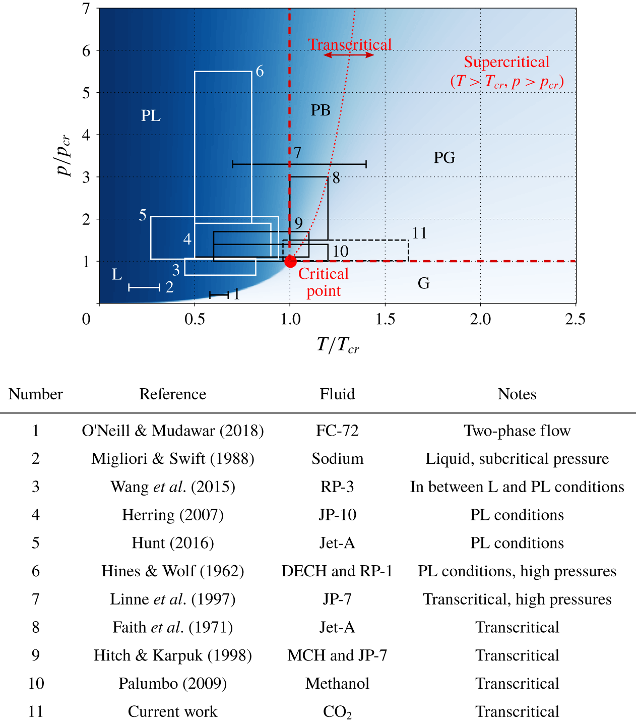
Generic state diagram showing the range of thermodynamic conditions with respect to the critical point  $(T=T_{cr},p=p_{cr})$ considered in previous studies of thermoacoustic instabilities involving either multiphase mixtures, liquids or supercritical fluids. The abbreviations L, PL, PB, PG and G stand for fluid in liquid, pseudo-liquid, pseudo-boiling, pseudo-gaseous and gaseous conditions, respectively.

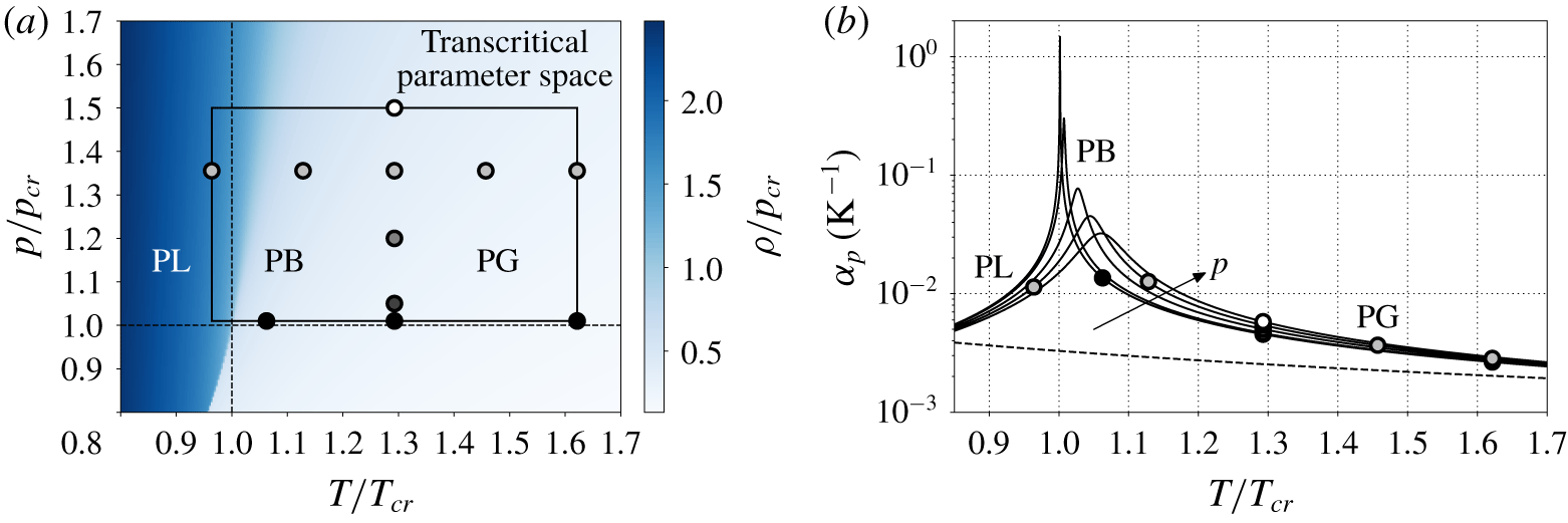
(a) Flooded contours of reduced density for  $\text{CO}_{2}$; (b) isobaric thermal expansion coefficient (1.3) versus reduced temperature for
 $\text{CO}_{2}$ at the pressures indicated in table 2. The rectangle drawn in (a) shows the parameter space of the linear stability analysis, while the 11 configurations of
 $T_{hot}$ and
 $p_{0}$ for the Navier–Stokes computations are indicated with circles. The curves in (b) are obtained with the PR EoS (solid lines) and with the perfect ideal gas EoS (dashed line,
 $1/T$).

Fluids in thermodynamic conditions close to their critical point are characterized by large thermal expansion coefficients, and their use would, theoretically, greatly increase the thermoacoustic gain in (1.2). In particular, for fluids in transcritical, or pseudo-boiling (PB) conditions (Fisher & Widom Reference Fisher and Widom1969; Tucker Reference Tucker1999; Banuti Reference Banuti2015), wave-induced compressions and dilatations could be so large that periodic transitions from liquid-like fluid (pseudo-liquid) to gas-like fluid (or pseudo-gas) would occur (see figures 1 and 2). Around the PB region, the highly nonlinear coupling between pressure, temperature and density (thermodynamic nonlinearity) has been proposed by Herring & Heister (Reference Herring and Heister2006) as the reason for undesired effects such as thermoacoustic instabilities in high-pressure combustion chambers (Casiano, Hulka & Yang Reference Casiano, Hulka and Yang2010; Poinsot & Veynante Reference Poinsot and Veynante2011) or bulk-mode oscillations in pressurized fuel heat exchangers (Hines & Wolf Reference Hines and Wolf1962; Faith, Ackerman & Henderson Reference Faith, Ackerman and Henderson1971; Linne et al. Reference Linne, Meyer, Edwards and Eitman1997; Hitch & Karpuk Reference Hitch and Karpuk1998; Herring Reference Herring2007; Palumbo Reference Palumbo2009; Hunt & Heister Reference Hunt and Heister2014; Wang et al. Reference Wang, Zhou, Pan and Wang2015; Hunt Reference Hunt2016), often leading to catastrophic hardware failure. These phenomena are similar to the multiphase instabilities called density wave oscillations (O’Neill & Mudawar Reference O’Neill and Mudawar2018). The regions of the phase space considered in the literature are shown in figure 1.
The use of a fluid close to its critical point in a thermoacoustic engine was already suggested by Swift (Reference Swift1988). In fact, the power energy density is proportional to  $\unicode[STIX]{x1D6FC}_{p_{0}}T_{0}$, making a high thermal expansion coefficient one of the basic requirements in the selection of the working fluid. However, the high pressures involved in the handling of transcritical fluids, together with the drop of their thermal diffusivity (hence requiring very small pore size in the heat exchangers and stack), has limited their use in a thermoacoustic engine so far (Alexander et al. Reference Alexander, Migliorino, Heister and Scalo2018). Moreover, high-fidelity numerical simulations of transcritical thermoacoustic instabilities have not been carried out yet. One of the major challenges is the use of fully conservative schemes (Karni Reference Karni1994; Abgrall Reference Abgrall1996; Toro Reference Toro2002), for which spurious numerical oscillations have been shown to produce unstable computations when transcritical flows are considered (Kawai, Terashima & Negishi Reference Kawai, Terashima and Negishi2015; Pantano, Saurel & Schmitt Reference Pantano, Saurel and Schmitt2017; Migliorino et al. Reference Migliorino, Chapelier, Scalo and Lodato2018). The most relevant previous work is the development of the linear thermoacoustic theory, applicable to a generic fluid, by Swift (Reference Swift1988), which builds upon classical linear theory (Kirchhoff Reference Kirchhoff1868; Kramers Reference Kramers1949; Rott Reference Rott1969). This theory was applied to the design of a thermoacoustic engine successfully operated with liquid sodium (Migliori & Swift Reference Migliori and Swift1988), which demonstrated that fluids other than ideal gases, and in particular liquids, which had been employed before in Malone-type Stirling-like engines (Malone Reference Malone1931), can be employed in thermoacoustic systems.
The objective of this work is to establish a numerical benchmark for high-fidelity simulations of transcritical thermoacoustic flows, extending previous efforts aimed at the understanding and description of canonical thermoacoustic instabilities (Scalo, Lele & Hesselink Reference Scalo, Lele and Hesselink2015; Lin, Scalo & Hesselink Reference Lin, Scalo and Hesselink2016; Gupta, Lodato & Scalo Reference Gupta, Lodato and Scalo2017). This goal is accomplished by investigating a standing-wave-like thermoacoustically unstable two-dimensional resonator with transcritical  $\text{CO}_{2}$ as the working fluid, building upon Migliorino, Gupta & Scalo (Reference Migliorino, Gupta and Scalo2017), idealizing the set-up used by Alexander et al. (Reference Alexander, Migliorino, Heister and Scalo2018).
The manuscript is organized as follows: the problem formulation (§ 2) starts with the fluid model and the thermodynamic conditions employed in the Navier–Stokes simulations (§ 2.1), followed by the description of the computational set-up (§ 2.2). The latter includes the full set of governing equations and the numerical set-up employed to solve them (§ 2.2.1), and the thermoviscous wave equations, which guide the geometry optimization (§ 2.2.2). The section ends with a grid sensitivity analysis (§ 2.3), showing the need to include the fully complex eigenvalue in the thermoviscous functions dependence. Real-fluid effects are then discussed in § 3, namely on the frequency and growth rate (§ 3.1), and on the eigenmode shapes in § 3.2, where the reasons for the flattening of the pressure eigenmode amplitude and the smooth transition of the pressure–velocity phase difference at the average location of the pressure node are explained. Then, the energy budgets are discussed in § 4, with a first focus on the acoustic energy budgets (§ 4.1) demonstrating how acoustic power production is increased when approaching the critical point, and then on the total energy budgets (§ 4.2), which show a similar increase also for the heat required. Finally, high amplitude pressure oscillations are first investigated in § 5 by discussing the thermodynamic and convective nonlinearities typical of fluids in transcritical states, and then by describing the limit cycle obtained due to nonlinear minor area losses (§ 6).
2 Problem formulation
2.1 Fluid model
In this work we have selected carbon dioxide as the working fluid because of its well documented properties (see table 1), making it a good choice for our theoretical investigation. Its transcritical, or PB, state is reached when the fluid is at pressures exceeding its critical value,  $p>p_{cr}$, and the temperature varies between
 $T<T_{cr}$ (pseudo-liquid conditions) and
 $T>T_{cr}$ (pseudo-gaseous conditions), as figure 2 shows. The density rapidly drops when transitioning from PL to PG conditions (figure 2a), hence the spike in the isobaric thermal expansion coefficient (figure 2b). However, for increasing pressures, this transition becomes more gradual, and, for large values of the temperature,
 $\unicode[STIX]{x1D6FC}_{p}$ tends to
 $1/T$, reverting to a perfect ideal gas behaviour.
Critical properties, molar mass and acentric factor of  $\text{CO}_{2}$.

Selected base pressures for the Navier–Stokes simulations.

Specific parameters for the PR EoS (2.1).

The parameter space considered in this study spans the range of base pressures  $p_{0}=1.01-1.5p_{cr}$ and temperature differences
 $\unicode[STIX]{x0394}T=T_{hot}-T_{cold}$ up to 200 K (figure 2a, see also (2.2), (2.3) and figure 3). For all cases, the value of the cold temperature is
 $T_{cold}=293.15~\text{K}$. Five base pressures (table 2) are taken into account for the Navier–Stokes simulations.
The equation of state (EoS) of Peng & Robinson (Reference Peng and Robinson1976) (PR EoS) and the model of Chung et al. (Reference Chung, Ajlan, Lee and Starling1988) for viscosity and thermal conductivity are chosen as the real-fluid model due to their simplicity and ease of implementation. The PR EoS relates pressure, density and temperature as follows:
 $$\begin{eqnarray}\displaystyle p=\frac{\unicode[STIX]{x1D70C}RT}{1-\unicode[STIX]{x1D70C}b}-\frac{\unicode[STIX]{x1D70C}^{2}\unicode[STIX]{x1D6FC}_{cr}\unicode[STIX]{x1D6FC}}{(1-\unicode[STIX]{x1D70C}c_{1}b)(1-\unicode[STIX]{x1D70C}c_{2}b)}, & & \displaystyle\end{eqnarray}$$
where  $R=R_{u}/M_{m}$,
 $M_{m}$ is the molar mass,
 $R_{u}=8.314472~\text{J}~\text{mol}^{-1}~\text{K}^{-1}$ is the universal gas constant, and
 $\unicode[STIX]{x1D6FC}$ is chosen as the one proposed by Soave (Reference Soave1972),
 $\sqrt{\unicode[STIX]{x1D6FC}}=1+\unicode[STIX]{x1D6FD}(1-\sqrt{T/T_{cr}})$. The other coefficients are listed in table 3. Notice that the EoS and transport parameter model degrade in accuracy for thermodynamic conditions close to the critical point, while still retaining all the important features of real fluids.
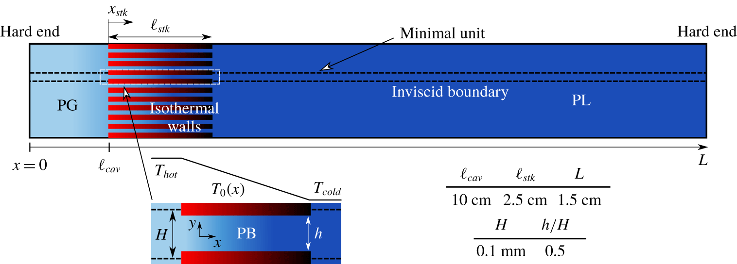
Computational set-up (not to scale) with geometrical parameters for minimal unit numerical simulations. Isothermal boundary conditions in the stack are imposed following (2.3). The sidewalls are considered adiabatic.

2.2 Computational set-up
The geometrical set-up considered in this study (figure 3) is a two-dimensional resonator composed of a hot cavity, indicated by the subscript  $cav$, a thermoacoustic stack, indicated by the subscript
 $stk$, and a long duct. The whole system is bounded axially by two adiabatic walls at
 $x=0$ and
 $x=L$. Fluid in PL conditions (
 $T_{cold}$) and PG conditions (
 $T_{hot}$), according to the base temperature distribution
 $$\begin{eqnarray}\displaystyle T_{0}(x)=\left\{\begin{array}{@{}ll@{}}T_{hot}\quad & 0\leqslant x\leqslant \ell _{cav},\\ T_{cold}\quad & \ell _{cav}+\ell _{stk}\leqslant x\leqslant L,\end{array}\right. & & \displaystyle\end{eqnarray}$$
bound the stack ( $0<x_{stk}<\ell _{stk}$), kept at PB conditions by isothermal wall boundary conditions, which impose the following temperature profile:
 $$\begin{eqnarray}\displaystyle T_{0}(x)=T_{hot}-\unicode[STIX]{x0394}Tx_{stk}/\ell _{stk}, & & \displaystyle\end{eqnarray}$$
where  $\unicode[STIX]{x0394}T=T_{hot}-T_{cold}$. The stack coordinate is defined as
 $$\begin{eqnarray}\displaystyle x_{stk}=x-\ell _{cav}. & & \displaystyle\end{eqnarray}$$
A canonical minimal unit (Gupta et al. Reference Gupta, Lodato and Scalo2017) is carved out of this geometry, defining the computational set-up employed for both the linear (frequency domain) and fully nonlinear (Navier–Stokes) numerical analyses. The definition of a minimal unit greatly reduces the computational cost of the Navier–Stokes simulations, which is especially high when employing transcritical fluids, and does not compromise the generality of the results obtained, provided that thermoviscous losses in the parts outside the stack are negligible. Such a condition is true when  $\unicode[STIX]{x1D6FF}_{k}/R\ll 1$, where
 $R$ is the hydraulic radius of the resonator and
 $\unicode[STIX]{x1D6FF}_{k}$ is the thermal boundary layer thickness (see (5.1)), and is verified for example in Alexander et al. (Reference Alexander, Migliorino, Heister and Scalo2018), where
 $\unicode[STIX]{x1D6FF}_{k}/R=3.84\times 10^{-3}$. This set-up takes into account nonlinear thermodynamic effects and hydrodynamic nonlinear losses due to area jumps, which will be analysed in § 5 and § 6, respectively. Acoustic streaming, transitional turbulence and nonlinear wave steepening are not considered in the Navier–Stokes simulations performed in this study.
2.2.1 Governing nonlinear equations and numerical set-up
In this work we consider the fully compressible Navier–Stokes equations, expressed by the conservation laws of mass and momentum,
 $$\begin{eqnarray}\displaystyle & \displaystyle \frac{\unicode[STIX]{x2202}\unicode[STIX]{x1D70C}}{\unicode[STIX]{x2202}t}+\frac{\unicode[STIX]{x2202}\unicode[STIX]{x1D70C}u_{j}}{\unicode[STIX]{x2202}x_{j}}=0, & \displaystyle\end{eqnarray}$$
 $$\begin{eqnarray}\displaystyle & \displaystyle \frac{\unicode[STIX]{x2202}\unicode[STIX]{x1D70C}u_{i}}{\unicode[STIX]{x2202}t}+\frac{\unicode[STIX]{x2202}\unicode[STIX]{x1D70C}u_{i}u_{j}}{\unicode[STIX]{x2202}x_{j}}=-\frac{\unicode[STIX]{x2202}p}{\unicode[STIX]{x2202}x_{i}}+\frac{\unicode[STIX]{x2202}\unicode[STIX]{x1D70F}_{ij}}{\unicode[STIX]{x2202}x_{j}}, & \displaystyle\end{eqnarray}$$
and the evolution equation for pressure (Migliorino & Scalo Reference Migliorino and Scalo2017),
 $$\begin{eqnarray}\displaystyle \frac{\unicode[STIX]{x2202}p}{\unicode[STIX]{x2202}t}+\frac{\unicode[STIX]{x2202}pu_{j}}{\unicode[STIX]{x2202}x_{j}}=(p-\unicode[STIX]{x1D70C}a^{2})\frac{\unicode[STIX]{x2202}u_{j}}{\unicode[STIX]{x2202}x_{j}}+\frac{a^{2}\unicode[STIX]{x1D6FC}_{p}}{c_{p}}\left(\unicode[STIX]{x1D70F}_{ij}\frac{\unicode[STIX]{x2202}u_{i}}{\unicode[STIX]{x2202}x_{j}}-\frac{\unicode[STIX]{x2202}q_{j}}{\unicode[STIX]{x2202}x_{j}}\right), & & \displaystyle\end{eqnarray}$$
where  $t$ is time,
 $x_{j}$ and
 $u_{j}$ (
 $j=1,2,3$) are the components of position and velocity,
 $\unicode[STIX]{x1D70C}$ and
 $p$ are the density and pressure,
 $a$ is the sound speed,
 $\unicode[STIX]{x1D6FC}_{p}$ is the isobaric thermal expansion coefficient (1.3) and
 $c_{p}$ is the isobaric specific thermal capacity. The Newtonian viscous stress tensor
 $\unicode[STIX]{x1D70F}_{ij}$, according to Stokes’s hypothesis, and the Fourier heat flux read, respectively,
 $$\begin{eqnarray}\displaystyle \unicode[STIX]{x1D70F}_{ij}=\unicode[STIX]{x1D707}\left(\frac{\unicode[STIX]{x2202}u_{i}}{\unicode[STIX]{x2202}x_{j}}+\frac{\unicode[STIX]{x2202}u_{j}}{\unicode[STIX]{x2202}x_{i}}-\frac{2}{3}\unicode[STIX]{x1D6FF}_{ij}\frac{\unicode[STIX]{x2202}u_{k}}{\unicode[STIX]{x2202}x_{k}}\right),\quad q_{j}=-k\frac{\unicode[STIX]{x2202}T}{\unicode[STIX]{x2202}x_{j}}, & & \displaystyle\end{eqnarray}$$
where  $\unicode[STIX]{x1D6FF}_{ij}$ is the Kronecker delta,
 $\unicode[STIX]{x1D707}$ is the dynamic viscosity,
 $k$ is the thermal conductivity and
 $T$ is the absolute temperature. Both
 $\unicode[STIX]{x1D707}$ and
 $k$ depend on density and temperature according to the model of Chung et al. (Reference Chung, Ajlan, Lee and Starling1988).
Equations (2.5), (2.6) and (2.7) are solved with the unstructured spectral difference (SD) solver sd3DvisP, the same as used by Gupta et al. (Reference Gupta, Lodato and Scalo2017) in their thermoacoustics simulations. It has been shown (Migliorino et al. Reference Migliorino, Chapelier, Scalo and Lodato2018) that solving for the total energy equation leads to numerical instability when simulating transcritical flows, due to the loss of mechanical equilibrium at contact discontinuities. Instead, solving the pressure evolution equation (2.7) ensures numerical stability and correct representation of the physics of low Mach number flows (Kawai et al. Reference Kawai, Terashima and Negishi2015), such as the ones considered in this study. This numerical approach has been tested and validated in Migliorino et al. (Reference Migliorino, Chapelier, Scalo and Lodato2018).
The Navier–Stokes numerical simulations are initialized with the following conditions:
 $$\begin{eqnarray}\displaystyle p=p_{0},\quad T=T_{0}(x),\quad u=\frac{p_{0}p_{amp}}{\unicode[STIX]{x1D70C}_{0}a_{0}}\sin (\unicode[STIX]{x03C0}x/L),\quad v=0, & & \displaystyle\end{eqnarray}$$
where  $T_{0}(x)$ is given by (2.2) and (2.3),
 $\unicode[STIX]{x1D70C}_{0}=\unicode[STIX]{x1D70C}_{0}(x)$ and
 $a_{0}=a_{0}(x)$ are the density and sound speed corresponding to
 $p_{0}$ and
 $T_{0}(x)$, respectively, and
 $p_{amp}=10^{-7}$ for all cases, apart from the ones analysed in § 5 and § 6, for which
 $p_{amp}=5\times 10^{-3}$. Equation (2.9) imposes an initial disturbance in the computational set-up that is thermoacoustically amplified if the system is fluid-dynamically unstable.
The effect of gravity is not taken into account in the present model. In fact, for horizontal or hot-side-up laboratory configuration, gravity will have no significant effect on the oscillating flow dynamics (Alexander et al. Reference Alexander, Migliorino, Heister and Scalo2018). If the set-up is placed hot-side-down, boiling might ensue, potentially disrupting any formation of thermoacoustic waves. By placing the hot side up, gravity can also be used to stabilize the mean profiles of temperature and density to avoid any mean flow induced by acoustic nonlinearities.
2.2.2 Linearized thermoviscous wave equations and geometry optimization
From (2.5), (2.6) and (2.7), it is possible (Rott Reference Rott1969; Swift et al. Reference Swift, Migliori, Hofler and Wheatley1985; Migliorino et al. Reference Migliorino, Gupta and Scalo2017) to obtain, for a generic duct, the frequency-domain equations for the complex volumetric flow rate  $\hat{U}$ and pressure
 $\hat{p}$ (see appendix A),
 $$\begin{eqnarray}\displaystyle & \displaystyle \unicode[STIX]{x1D70E}\hat{U} =-\frac{A}{\unicode[STIX]{x1D70C}_{0}F_{\unicode[STIX]{x1D708}}}\frac{\text{d}\hat{p}}{\text{d}x}, & \displaystyle\end{eqnarray}$$
 $$\begin{eqnarray}\displaystyle & \displaystyle \unicode[STIX]{x1D70E}\hat{p}=\frac{\unicode[STIX]{x1D70C}_{0}a_{0}^{2}}{AF_{k}}\left(\unicode[STIX]{x1D6E9}\unicode[STIX]{x1D6F7}_{{\mathcal{P}}}-\frac{\text{d}}{\text{d}x}\right)\hat{U} , & \displaystyle\end{eqnarray}$$
 $\unicode[STIX]{x1D70E}=\unicode[STIX]{x1D6FC}+\text{i}\unicode[STIX]{x1D714}$ is the complex eigenvalue with growth rate
 $\unicode[STIX]{x1D6FC}$ and angular frequency
 $\unicode[STIX]{x1D714}$, and
 $$\begin{eqnarray}\displaystyle \unicode[STIX]{x1D6F7}_{{\mathcal{P}}}=\frac{1}{1-Pr_{0}}\frac{f_{k}-f_{\unicode[STIX]{x1D708}}}{1-f_{\unicode[STIX]{x1D708}}},\quad F_{\unicode[STIX]{x1D708}}=\frac{1}{1-f_{\unicode[STIX]{x1D708}}},\quad F_{k}=1+(\unicode[STIX]{x1D6FE}_{0}-1)f_{k}, & & \displaystyle\end{eqnarray}$$
where the thermoviscous functions  $f_{\unicode[STIX]{x1D708}}$ and
 $f_{k}$ depend on
 $\unicode[STIX]{x1D70E}$, the duct geometry, Prandtl number and kinematic viscosity (see (A 21) and (A 31)). Base state quantities are a function of the axial coordinate
 $x$ only and are denoted with a subscript 0;
 $\unicode[STIX]{x1D708}_{0}=\unicode[STIX]{x1D707}_{0}/\unicode[STIX]{x1D70C}_{0}$ is the kinematic viscosity,
 $\unicode[STIX]{x1D6FE}_{0}=c_{p_{0}}/c_{v_{0}}$ is the ratio of specific heats and
 $Pr_{0}=c_{p_{0}}\unicode[STIX]{x1D707}_{0}/k_{0}$ is the Prandtl number. Furthermore,
 $A$ is in general the cross-sectional area of the duct, intended per unit depth for the geometry employed in this study. When the linearized equations are solved, the flow field is considered at uniform base pressure
 $p_{0}$.
Equations (2.10a) and (2.10b) are discretized on a staggered uniform grid with second-order numerical operators (Lin et al. Reference Lin, Scalo and Hesselink2016; Gupta et al. Reference Gupta, Lodato and Scalo2017) and solved with a shift-Arnoldi algorithm. For all the results in this paper, we will always refer to the first resonant mode of the system.
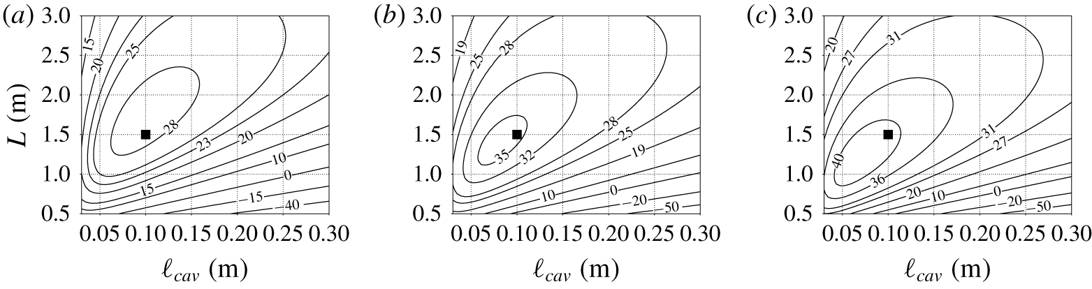
The minimal unit computational set-up is optimized, based on the linear theory, for three values of  $\unicode[STIX]{x0394}T$ (figure 4), resulting in the geometrical parameters listed in figure 3. The optimization is performed here visually on the plots of the growth rates and provides a geometry for which thermoacoustic instability appears for only approximately
 $\unicode[STIX]{x0394}T=25~\text{K}$. Other values of
 $p_{0}$ or
 $\unicode[STIX]{x0394}T$ considered in the optimization would lead to different geometries, which are not considered in this study.
Isolevels of thermoacoustic growth rate,  $\unicode[STIX]{x1D6FC}$ (
 $\text{rad}~\text{s}^{-1}$), versus total length,
 $L$, and length of the hot cavity,
 $\ell _{cav}$ (see figure 3), for
 $p_{0}=10~\text{MPa}$,
 $\unicode[STIX]{x0394}T=100~\text{K}$ (a),
 $\unicode[STIX]{x0394}T=125~\text{K}$ (b), and
 $\unicode[STIX]{x0394}T=150~\text{K}$ (c), with a black square indicating the selected design point. These results are obtained with the solution of the linear system of equations composed by (2.10a) and (2.10b).

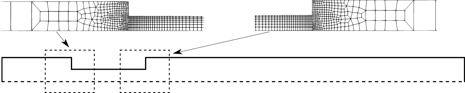
Illustrations of portions of the unstructured mesh for grid B (see table 4), close to area changes, used for the Navier–Stokes simulations. This mesh has total number of elements  $N_{el}=2635$.

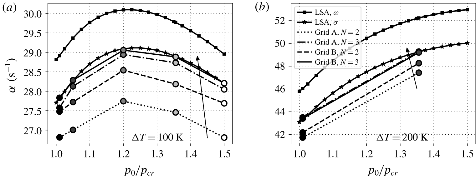
Growth rate versus reduced base pressure for  $\unicode[STIX]{x0394}T=100~\text{K}$ (a) and
 $\unicode[STIX]{x0394}T=200~\text{K}$ (b), for the different grid resolutions in table 4. Circles connected by lines are obtained from the Navier–Stokes simulations, with arrows indicating increasing resolution (see legend in (b)). Results labelled with ‘LSA,
 $\unicode[STIX]{x1D714}$’ and ‘LSA,
 $\unicode[STIX]{x1D70E}$’ are obtained from linear stability analysis (LSA) with thermoviscous functions only dependent on
 $\unicode[STIX]{x1D714}$ (2.13), and on
 $\unicode[STIX]{x1D6FC}+\text{i}\unicode[STIX]{x1D714}$ (2.12), respectively.

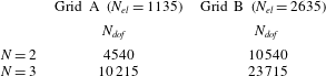
Number of degrees of freedom,  $N_{dof}=N^{2}N_{el}$, for the two grids considered in this study, and for two numbers of solution points
 $N$ inside each element.

2.3 Grid sensitivity analysis
The Navier–Stokes simulations are carried out on an unstructured mesh discretizing only half of the minimal unit (figure 5), exploiting the symmetry of the flow field with respect to the centre line of the domain. Two different grids are considered (table 4): A (coarse) and B (fine). The order of accuracy of the polynomial reconstruction is fixed with  $N$, indicating the number of points inside each element. For each grid,
 $N=2$ and
 $N=3$ are chosen.
A grid sensitivity study on the linear growth rate indicates converging behaviour (figure 6) of the data from the Navier–Stokes simulations, from grid A with  $N=2$ to the finest resolution employed (grid B and
 $N=3$), towards the growth rates predicted by the linear theory. However, an important remark is that to achieve such agreement the thermoviscous functions in (A 21) and (A 31) have to depend on the full eigenvalue
 $\unicode[STIX]{x1D70E}$, and not only on its imaginary part
 $\unicode[STIX]{x1D714}$, otherwise linear theory overpredicts the growth rate. In fact, the normalization for the transverse spatial coordinate
 $r$, equation (A 16), which reads
 $$\begin{eqnarray}\displaystyle \unicode[STIX]{x1D702}=\sqrt{\frac{\unicode[STIX]{x1D70E}}{\unicode[STIX]{x1D708}_{0}}}r=\sqrt{2\text{i}+2\frac{\unicode[STIX]{x1D6FC}}{\unicode[STIX]{x1D714}}}\frac{r}{\unicode[STIX]{x1D6FF}_{\unicode[STIX]{x1D708}}}, & & \displaystyle\end{eqnarray}$$
where  $\unicode[STIX]{x1D6FF}_{\unicode[STIX]{x1D708}}$ is defined in (5.1), includes both the growth rate,
 $\unicode[STIX]{x1D6FC}$, and angular frequency,
 $\unicode[STIX]{x1D714}$, information. Previous studies restricted to ideal gas (Rott Reference Rott1969; Swift et al. Reference Swift, Migliori, Hofler and Wheatley1985; Lin et al. Reference Lin, Scalo and Hesselink2016; Gupta et al. Reference Gupta, Lodato and Scalo2017) have made the assumption that
 $\unicode[STIX]{x1D6FC}\ll \unicode[STIX]{x1D714}$, i.e.
 $\unicode[STIX]{x1D70E}\approx \text{i}\unicode[STIX]{x1D714}$, which cannot be used here (see appendix B), yielding
 $$\begin{eqnarray}\displaystyle \unicode[STIX]{x1D702}=\sqrt{\frac{\text{i}\unicode[STIX]{x1D714}}{\unicode[STIX]{x1D708}_{0}}}r=\sqrt{2i}\frac{r}{\unicode[STIX]{x1D6FF}_{\unicode[STIX]{x1D708}}}=(i+1)\frac{r}{\unicode[STIX]{x1D6FF}_{\unicode[STIX]{x1D708}}}. & & \displaystyle\end{eqnarray}$$
Adopting  $N=3$ solution points yields approximately the same growth rates for grids A and B (especially for
 $\unicode[STIX]{x0394}T=200~\text{K}$, for which the two results are almost identical). Furthermore, an almost equal number of total degrees of freedom
 $N_{dof}$ entails different results depending on the order of the polynomial reconstruction inside each element: grid A with
 $N=3$ (
 $N_{dof}=10\,215$) provides a better estimate of the growth rates compared to grid B with
 $N=2$ (
 $N_{dof}=10\,540$). This justifies the use of high-order numerics in the simulation of thermoacoustic instabilities.
Frequencies were found to be not very sensitive to grid resolution, as they are determined primarily from inviscid processes.
3 Real-fluid effects on frequency, growth and eigenmodes
3.1 Real-fluid effects on frequency and growth rate
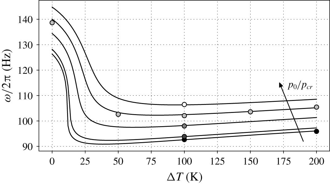
The frequency of the thermoacoustic response is dependent on the  $\unicode[STIX]{x0394}T$ across the stack for all base pressures
 $p_{0}$ considered (figure 7). The largest values of
 $\unicode[STIX]{x1D714}$ are obtained for values of
 $\unicode[STIX]{x0394}T$ below 5 K, for which most of the system is filled with pseudo-liquid, which has a high speed of sound. Then, for increasing
 $\unicode[STIX]{x0394}T$, the frequency drops by approximately 40 %, with sharper variations at near-critical conditions, due to the drop in sound speed characteristic of PB fluids. For higher values of
 $\unicode[STIX]{x0394}T$, the frequency increases approximately in a linear fashion, due to the appearance of fluid in near-ideal gas state, for which the speed of sound increases with temperature, in the hot cavity. Keeping the same
 $\unicode[STIX]{x0394}T$ across the stack, for increasing base pressures, the frequency increases approximately with a linear trend, entailing changes of 15 % from
 $p/p_{cr}=1.01$ to
 $1.5$. Thermoacoustic oscillations featuring ideal gases show much milder dependence of the frequency on the thermodynamic conditions (Lin et al. Reference Lin, Scalo and Hesselink2016; Gupta et al. Reference Gupta, Lodato and Scalo2017). The grid requirements necessary to capture the correct frequency are less stringent than the ones needed for numerical convergence of the growth rates (figure 6).


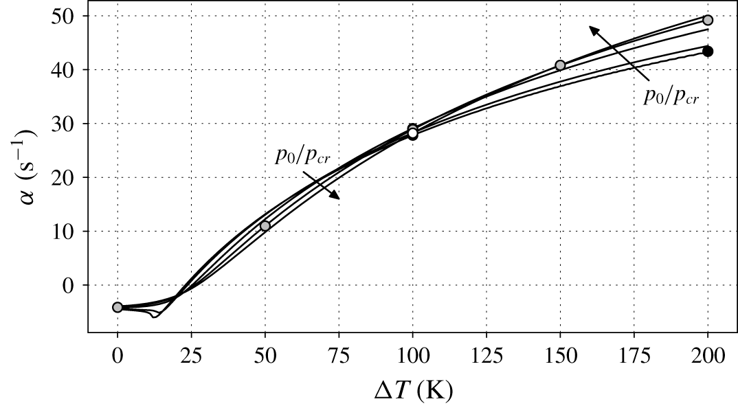
The thermoacoustic growth rate strongly depends on the  $\unicode[STIX]{x0394}T$ across the stack (figure 8), because large values of
 $\unicode[STIX]{x0394}T$ increase the thermoacoustic gain
 $\unicode[STIX]{x1D6E9}$, which in turn controls the acoustic energy production (discussed more in detail in § 4.1). For all base pressures considered, the minimum
 $\unicode[STIX]{x0394}T$ required for the onset of instability (positive growth rate) is only approximately
 $25~\text{K}$, much less than what is usually needed in standard thermoacoustic systems employing perfect ideal gases (Swift Reference Swift1992; Lin et al. Reference Lin, Scalo and Hesselink2016; Gupta et al. Reference Gupta, Lodato and Scalo2017). The configuration with base pressure closer to the critical pressure requires the lowest
 $\unicode[STIX]{x0394}T~(=23~\text{K})$ to be thermoacoustically unstable.
A non-monotonic variation in the growth rate is present right before  $\unicode[STIX]{x0394}T=15~\text{K}$, for
 $p_{0}=1.01p_{cr}$ and
 $p_{0}=1.05p_{cr}$, due to the occurrence of PB conditions inside the stack, whereas higher values of
 $p_{0}$ entail the monotonic trends expected in ideal gases. From the onset of instability onwards, increasing
 $\unicode[STIX]{x0394}T$ always corresponds to a rise in growth rate, with the highest values obtained in near-critical conditions (for the lowest values of
 $p_{0}$ considered) until approximately 100 K; after such a value, the growth rate monotonically increases with pressure. The latter is a surprising result if one simply relies on the intuition that higher base density gradients, achieved at lower pressures, are expected to boost thermoacoustic energy production (Migliorino et al. Reference Migliorino, Gupta and Scalo2017). Instead, for example, at
 $\unicode[STIX]{x0394}T=100~\text{K}$ the growth rate varies in a non-monotonic manner with different base pressures, showing a maximum around
 $p_{0}=1.25p_{cr}$ (figure 6a), which will be explained in § 4.1. These effects are not usually present in thermoacoustic systems employing ideal gases (Swift Reference Swift1992; Lin et al. Reference Lin, Scalo and Hesselink2016; Gupta et al. Reference Gupta, Lodato and Scalo2017).
Overall, the frequencies and growth rates extracted from the Navier–Stokes simulations confirm the predictions obtained from the linear theory, hence validating the linear ansatz despite the large gradients in the base state and the extreme thermodynamic conditions.
3.2 Real-fluid effects on eigenmodes
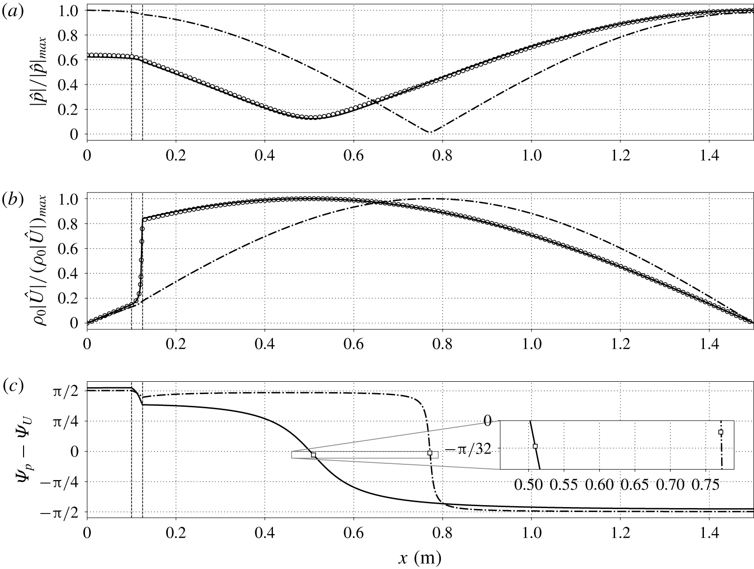
Strong real-fluid effects, due to the sharp base density gradients present in the stack, entail a deviation of the eigenmodes shapes from the classic ideal gas axial profiles (figure 9a,b). For  $\unicode[STIX]{x0394}T=200~\text{K}$, the overall spatial distribution of the eigenmodes, and their matching with Navier–Stokes data, were found not to be significantly dependent on
 $p_{0}$.
Axial distribution of pressure (a) and mass flow rate (b) dimensionless amplitudes and phasing between  $\hat{p}$ and
 $\hat{U}$ (c), for
 $\unicode[STIX]{x0394}T=200~\text{K}$ and
 $p_{0}=10~\text{MPa}$: linear theory (solid lines), data extracted from the Navier–Stokes simulations (circles). Dashed-dotted lines indicate eigenmodes obtained from linear theory with the assumption of thermally perfect ideal gas. Vertical dashed lines indicate locations of abrupt area change (see figure 3). The squares in (c) indicate values of phase difference at the location of minimum pressure amplitude.

The spatial variation of the amplitude of the pressure eigenmode in the linear regime (figure 9a) is much more gradual than its ideal gas counterpart. This can be explained (appendix B) as a result of the closure of the acoustic energy budgets, yielding
 $$\begin{eqnarray}\displaystyle \frac{|\hat{p}|_{min}}{|\hat{p}|_{max}}\propto \frac{|\unicode[STIX]{x1D6FC}|}{\unicode[STIX]{x1D714}}, & & \displaystyle\end{eqnarray}$$
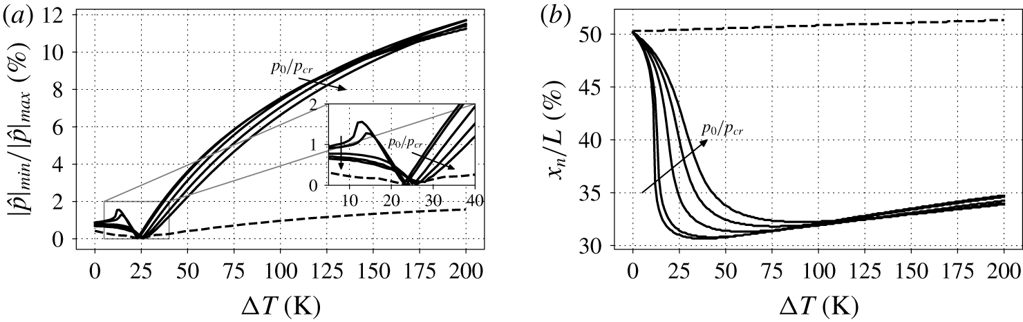
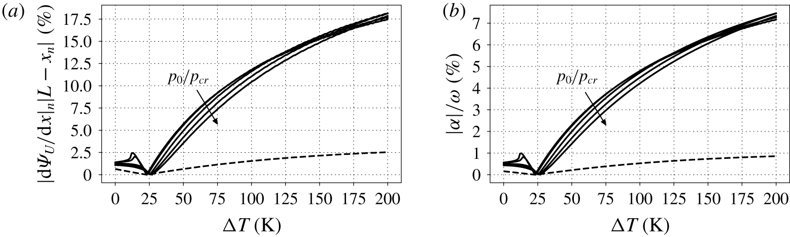
regardless of the EoS. A large growth-rate-to-frequency ratio is, however, typical of transcritical thermoacoustic oscillations (see figure 21b), with  $|\hat{p}|_{min}/|\hat{p}|_{max}$ values up to
 $12\,\%$ (figure 10a). The same configuration, with the assumption of a thermally perfect ideal gas, is characterized by
 $|\hat{p}|_{min}/|\hat{p}|_{max}$ values of at most
 $2\,\%$.
Furthermore, during the linear growth regime, a stationary node does not exist (see appendix B for more details), since the pressure eigenmode is zero at different axial locations in time. The average location of the pressure node is referred to as  $x=x_{|p|_{min}}=x_{n}$. In the transcritical case, the pressure eigenmode amplitude presents its minimum always shifted towards the stack (showing a minimum of approximately
 $31\,\%$ of the total length, see figure 10b), contrary to the ideal gas case, for which
 $x_{n}$ can reach a maximum of
 $0.51L$. The trend of
 $x_{n}$ versus
 $\unicode[STIX]{x0394}T$ resembles the one of frequency versus
 $\unicode[STIX]{x0394}T$ (figure 7). This is due to a local decrease in wavelength connected to the lower speed of sound of PB and PG conditions compared to PL conditions.
Data from linear stability theory on pressure eigenmode amplitude: relative magnitude (a) and location (b) of its minimum. Solid lines are for real-fluid EoS (for all base pressures in table 2), and the dashed line indicates thermally perfect ideal gas EoS (for  $p_{0}=10~\text{MPa}$ only).

In addition, the most intense mass transport events are expected inside the stack, where the axial gradient of  $\unicode[STIX]{x1D70C}_{0}|U|$ is maximum, which is where transcritical conditions are achieved (figure 9b). Such events, if pressure amplitudes are sufficiently high, entail convective nonlinearities (analysed in § 5).
Another quantity of interest is the phasing between  $\hat{p}$ and
 $\hat{U}$:
 $\unicode[STIX]{x1D6F9}_{p}-\unicode[STIX]{x1D6F9}_{U}$ (figure 9c). The axial profile of
 $\unicode[STIX]{x1D6F9}_{p}-\unicode[STIX]{x1D6F9}_{U}$, for the ideal gas configuration, is consistent with similar trends reported by Yazaki et al. (Reference Yazaki, Iwata, Maekawa and Tominaga1998), who observed a sharp change from
 $\unicode[STIX]{x03C0}/2$ to approximately
 $-\unicode[STIX]{x03C0}/2$. Instead, for the transcritical case,
 $\unicode[STIX]{x1D6F9}_{p}-\unicode[STIX]{x1D6F9}_{U}$ shows a much milder transition inside the resonator. Moreover, the value of
 $\unicode[STIX]{x1D6F9}_{p}-\unicode[STIX]{x1D6F9}_{U}$ at
 $x=x_{n}$ (see inset in figure 9c) is never exactly zero in the presence of thermoacoustic growth, and is in magnitude higher for the transcritical fluid than for the ideal gas case. In fact, it can be shown that (appendix B)
 $$\begin{eqnarray}\displaystyle \unicode[STIX]{x1D6F9}_{p_{n}}-\unicode[STIX]{x1D6F9}_{U_{n}}=-\arctan \left(\frac{\unicode[STIX]{x1D6FC}}{\unicode[STIX]{x1D714}}\right), & & \displaystyle\end{eqnarray}$$
indicating that the pressure–velocity phase difference is significantly different than zero at  $x=x_{n}$ for transcritical flows, due to the high value of
 $\unicode[STIX]{x1D6FC}/\unicode[STIX]{x1D714}$. This means that, at
 $x=x_{n}$, pressure and flow rate are generally more out of phase for transcritical fluids than for ideal gases. However, due to the smooth spatial variation in phasing, transcritical fluids exhibit a wider interval, centred around
 $x_{n}$, where travelling-wave-like phasing is present.
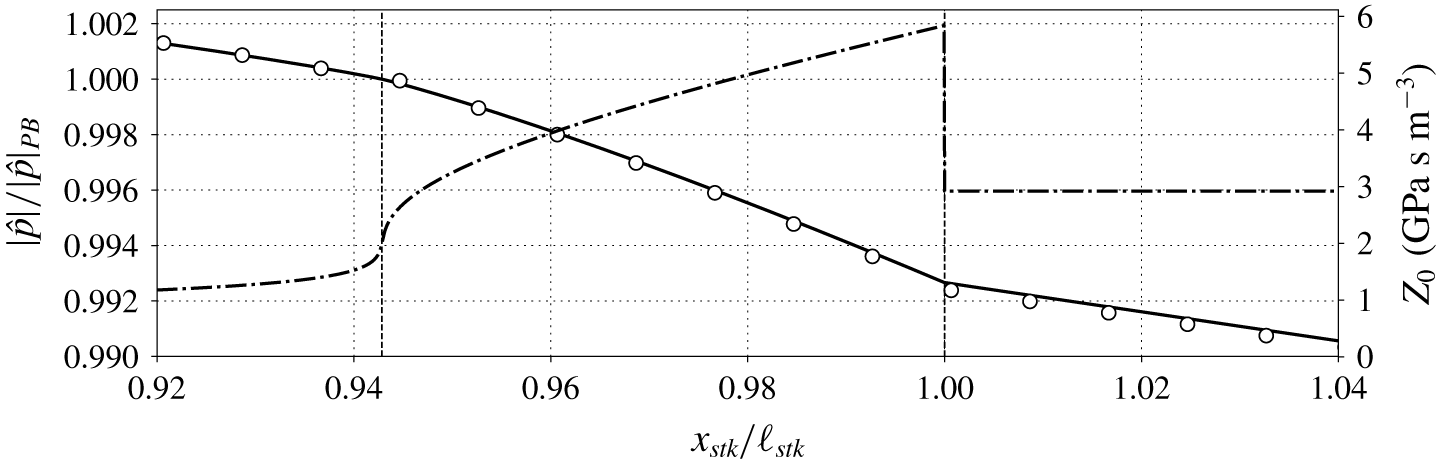
Axial distribution of dimensionless pressure amplitudes (left  $y$ axis), and base acoustic impedance (right
 $y$ axis), for
 $\unicode[STIX]{x0394}T=200~\text{K}$ and
 $p_{0}=1.01p_{cr}$: linear theory (solid line), data extracted from the Navier–Stokes simulations (circles), and base acoustic impedance (dashed dotted line). The vertical dashed line on the left indicates PB conditions, achieved at
 $x_{stk}/\ell _{stk}=0.942$, while the one on the right denotes the end of the stack (
 $x_{stk}/\ell _{stk}=1$).

We finally concentrate our attention towards the end of the stack, where we observe two changes in derivative of the pressure eigenmode amplitude (figure 11). These can be explained by considering the axial profiles of the acoustic impedance  $Z_{0}$, obtained as the ratio of the specific acoustic impedance and the duct area,
 $$\begin{eqnarray}\displaystyle Z_{0}=\frac{\unicode[STIX]{x1D70C}_{0}a_{0}}{A}. & & \displaystyle\end{eqnarray}$$
At  $x_{stk}/\ell _{stk}=1$, since no discontinuity in base state quantities is present (uniform
 $\unicode[STIX]{x1D70C}_{0}a_{0}$), the area change is responsible for a jump in
 $Z_{0}$, resulting in a local change in
 $\text{d}|\hat{p}|/\text{d}x$, also for the ideal gas case (not shown). However, no variations in area are present inside the stack, but in the vicinity of the pseudo-boiling region great variations of base density and speed of sound produce a pseudo-jump in
 $Z_{0}$, which entails a gradual change in the spatial derivative of the pressure eigenmode amplitude (and of the mass flow rate, not shown). This rapid change in
 $Z_{0}$ at transcritical conditions effectively acts on the eigenmodes like a continuous change in geometry, which is a peculiar real-fluid effect not present for higher base pressures or ideal gases, characterized by milder variations of thermodynamic properties.
The large difference in acoustic impedance between fluid in PL conditions and fluid in the hot cavity is also responsible for the presence of the maximum of pressure on the right end side of the domain for the real gas configuration (figure 9a). For ideal gases, instead, the acoustic impedance in the hot cavity can be higher than the one evaluated on the right of the stack, causing the maximum pressure amplitude to be at  $x=0$.
4 Energy budgets in the linear regime
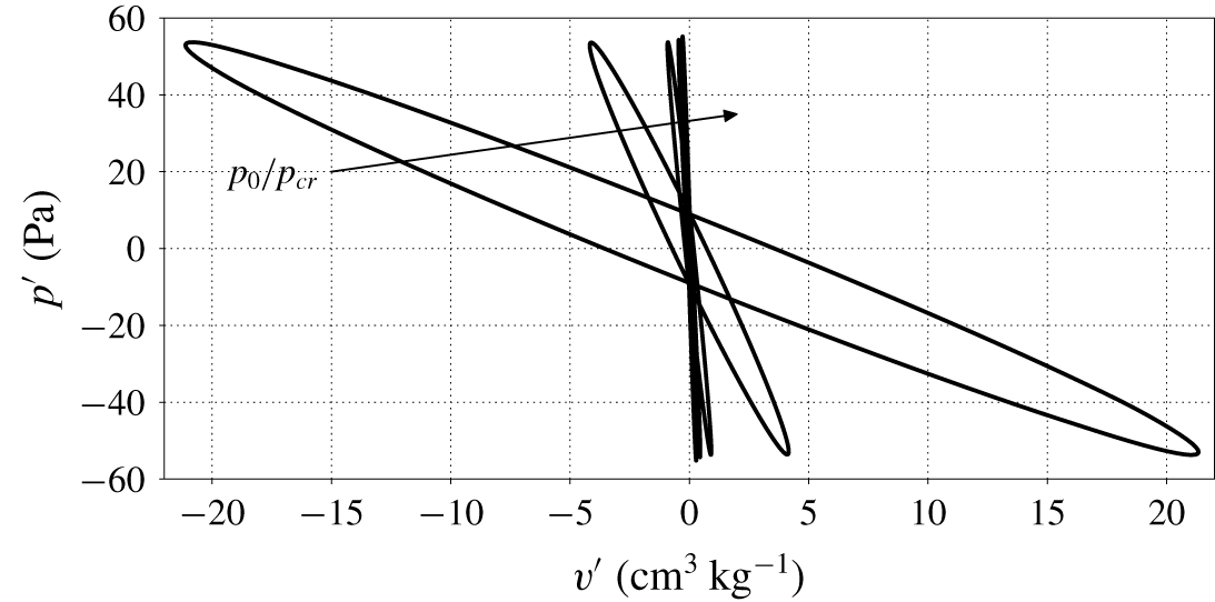
The mechanisms of conversion from heat to acoustic energy occur inside the stack, where a Lagrangian fluid parcel experiences a thermodynamic cycle, driven by the harmonic pressure oscillations, with expansions and contractions accompanied by heating and cooling. The resulting Lagrangian pressure–volume cycle, traversed clockwise, indicates mechanical power production (figure 12), which is strongly dependent on the spatial variation in the fluid’s base state resulting from the imposed mean temperature distribution (2.2). As base pressures approach the critical pressure, transcritical conditions entail sharper spatial gradients in base density, which in turn cause larger volume fluctuations for the same pressure oscillation amplitude, hence generating more power due to the larger area encompassed by the Lagrangian pressure–volume cycle.
Fluctuating pressure plotted against specific volume fluctuation of a Lagrangian fluid parcel, for all base pressures of table 2 and  $\unicode[STIX]{x0394}T=100~\text{K}$, extracted with the aid of the linear theory. Initial position of the Lagrangian parcel is at the centre line of the stack and at PB conditions (
 $x=12.21,12.17,12.019,11.88,11.77~\text{cm}$ for increasing values of
 $p_{0}$). All cycles are taken at the same pressure amplitude and are traversed clockwise.

4.1 Acoustic energy budgets
Multiplying (2.10a) by  $\hat{U} ^{\ast }$ and (2.10b) by
 $\hat{p}^{\ast }$, where a superscript
 $\ast$ indicates the complex conjugate, yields, after rearranging,
 $$\begin{eqnarray}\displaystyle & \displaystyle \unicode[STIX]{x1D70E}\overline{\unicode[STIX]{x1D705}}F_{\unicode[STIX]{x1D708}}A=-\frac{1}{2}\frac{\text{d}\hat{p}}{\text{d}x}\hat{U} ^{\ast }, & \displaystyle\end{eqnarray}$$
 $$\begin{eqnarray}\displaystyle & \displaystyle \unicode[STIX]{x1D70E}\overline{\unicode[STIX]{x1D700}}F_{k}A=\frac{\unicode[STIX]{x1D6E9}\unicode[STIX]{x1D6F7}_{{\mathcal{P}}}}{2}\hat{U} \hat{p}^{\ast }-\frac{1}{2}\hat{p}^{\ast }\frac{\text{d}\hat{U} }{\text{d}x}, & \displaystyle\end{eqnarray}$$
 $$\begin{eqnarray}\displaystyle \overline{\unicode[STIX]{x1D705}}=\frac{\unicode[STIX]{x1D70C}_{0}}{2}\frac{|\hat{U} |^{2}}{A^{2}},\quad \overline{\unicode[STIX]{x1D700}}=\frac{1}{2}\frac{|\hat{p}|^{2}}{\unicode[STIX]{x1D70C}_{0}a_{0}^{2}}, & & \displaystyle\end{eqnarray}$$
respectively, both with units of energy per unit volume. Taking the real part of the addition of (4.1a) with (4.1b), and using the properties  $\text{Re}\{\unicode[STIX]{x1D719}\unicode[STIX]{x1D713}\}=\text{Re}\{\unicode[STIX]{x1D719}\}\text{Re}\{\unicode[STIX]{x1D713}\}-\text{Im}\{\unicode[STIX]{x1D719}\}\text{Im}\{\unicode[STIX]{x1D713}\}$, and
 $\text{Re}\{\unicode[STIX]{x1D719}-\unicode[STIX]{x1D719}^{\ast }\}=0$, where
 $\unicode[STIX]{x1D719},\unicode[STIX]{x1D713}$ are two generic complex numbers, yields
 $$\begin{eqnarray}\displaystyle \unicode[STIX]{x1D6FC}\overline{{\mathcal{E}}}+\frac{\text{d}\overline{{\dot{W}}}}{\text{d}x}=\overline{{\mathcal{P}}}-\overline{{\mathcal{D}}}, & & \displaystyle\end{eqnarray}$$
where the acoustic energy density is defined as
 $$\begin{eqnarray}\displaystyle \overline{{\mathcal{E}}}=A(\text{Re}\{F_{\unicode[STIX]{x1D708}}\}\overline{\unicode[STIX]{x1D705}}+\text{Re}\{F_{k}\}\overline{\unicode[STIX]{x1D700}}), & & \displaystyle\end{eqnarray}$$
which has dimensions of an energy per unit length, the acoustic power is
 $$\begin{eqnarray}\displaystyle \overline{{\dot{W}}}={\textstyle \frac{1}{2}}\text{Re}\{\hat{p}\,\hat{U} ^{\ast }\}, & & \displaystyle\end{eqnarray}$$
which has dimensions of an energy per unit time, the production of acoustic energy density is
 $$\begin{eqnarray}\displaystyle \overline{{\mathcal{P}}}=\frac{\unicode[STIX]{x1D6E9}}{2}[\text{Re}\{\unicode[STIX]{x1D6F7}_{{\mathcal{P}}}\}\text{Re}\{\hat{p}^{\ast }\hat{U} \}-\text{Im}\{\unicode[STIX]{x1D6F7}_{{\mathcal{P}}}\}\text{Im}\{\hat{p}^{\ast }\hat{U} \}], & & \displaystyle\end{eqnarray}$$
and its dissipation is
 $$\begin{eqnarray}\displaystyle \overline{{\mathcal{D}}}=-\unicode[STIX]{x1D714}A(\text{Im}\{F_{\unicode[STIX]{x1D708}}\}\overline{\unicode[STIX]{x1D705}}+\text{Im}\{F_{k}\}\overline{\unicode[STIX]{x1D700}}), & & \displaystyle\end{eqnarray}$$
both with dimensions of power per unit length. The weights of  $\text{Re}\{\hat{p}^{\ast }\hat{U} \}$ and
 $\text{Im}\{\hat{p}^{\ast }\hat{U} \}$ in (4.6),
 $\text{Re}\{\unicode[STIX]{x1D6F7}_{{\mathcal{P}}}\}$ and
 $-\text{Im}\{\unicode[STIX]{x1D6F7}_{{\mathcal{P}}}\}$, respectively, are strongly dependent on
 $Pr_{0}$, but never negative (Migliorino et al. Reference Migliorino, Gupta and Scalo2017).
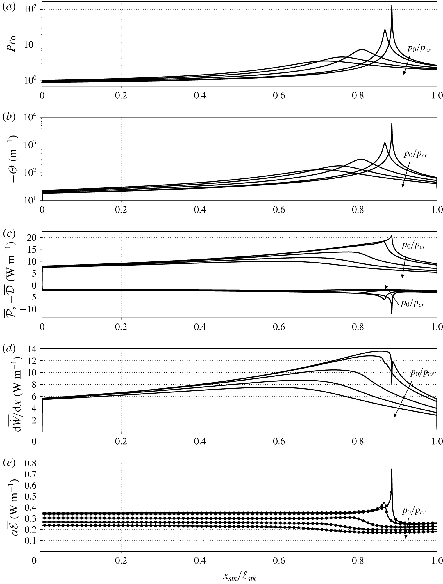
Base state quantities and acoustic energy budgets terms inside the stack ( $x_{stk}=[0,\ell _{stk}]$) from linear theory, for
 $\unicode[STIX]{x0394}T=100~\text{K}$ and the base pressures in table 2: (a) base Prandtl number; (b) minus thermoacoustic gain (1.1); (c) acoustic energy production ((4.6), positive values) and minus acoustic energy dissipation ((4.7), negative values); (d) axial gradient of acoustic power (4.5); (e)
 $\overline{{\mathcal{P}}}-\overline{{\mathcal{D}}}-\text{d}\overline{{\dot{W}}}/\text{d}x$ (filled circles) and
 $\unicode[STIX]{x1D6FC}\overline{{\mathcal{E}}}$ (solid lines, equation (4.4)), see (4.3). All quantities correspond to maximum pressure oscillation amplitude of 100 kPa, fixed for all base pressures.

Integrating (4.3) axially along the domain yields
 $$\begin{eqnarray}\displaystyle \unicode[STIX]{x1D6FC}={\mathcal{R}}/\unicode[STIX]{x1D6F4}, & & \displaystyle\end{eqnarray}$$
where the Rayleigh index (Gupta et al. Reference Gupta, Lodato and Scalo2017) is
 $$\begin{eqnarray}\displaystyle {\mathcal{R}}=\int _{0}^{L}(\overline{{\mathcal{P}}}-\overline{{\mathcal{D}}})\,\text{d}x, & & \displaystyle\end{eqnarray}$$
and the total acoustic energy is
 $$\begin{eqnarray}\displaystyle \unicode[STIX]{x1D6F4}=\int _{0}^{L}\overline{{\mathcal{E}}}\,\text{d}x, & & \displaystyle\end{eqnarray}$$
and where hard-wall boundary conditions have been taken into account (the acoustic power is zero at  $x=0$ and
 $x=L$). Once the eigenvalue problem in (2.10) is solved, it is possible to directly evaluate all the variables in (4.5), (4.6) and (4.7), allowing us to compute the growth rate from (4.8). This procedure has been carried out for all the configurations considered in this work and the growth rate hence obtained is in excellent agreement with the one computed from the numerical eigenvalue solution of (2.10). Indeed, the pointwise acoustic energy budgets in (4.3) are closed (figure 13e), corroborating the validity of the data extracted from the linear theory.
As the base pressure increases, transcritical conditions are achieved for a higher temperature (see figure 2b), shifting the location of fluid in PB conditions towards the hot side of the stack, and yielding a lower maximum of  $|\unicode[STIX]{x1D6E9}|$ (figure 13b). This directly affects the location and intensity of the spike of the acoustic energy production (figure 13c, equation (4.6)). The boost of production obtained for values of
 $p_{0}$ approaching
 $p_{cr}$ is, however, also accompanied by a similar increase in acoustic dissipation (figure 13c), due to the high values of Prandtl number typical of transcritical conditions (figure 13a). The nonlinear trends exhibited by production and dissipation of acoustic energy throughout the stack are responsible for the non-monotonic behaviour observed for the growth rate as a function of
 $p_{0}/p_{cr}$ in figure 6(a). Furthermore, the derivative of the acoustic power presents a maximum at PB conditions for higher base pressures, and a local minimum for
 $p_{0}=1.01p_{cr}$ and
 $p_{0}=1.05p_{cr}$. The acoustic energy density is mostly uniform in the stack, apart from the PB region where it presents a spike (figure 13e), gradually reduced by increasing the base pressures away from the critical point.
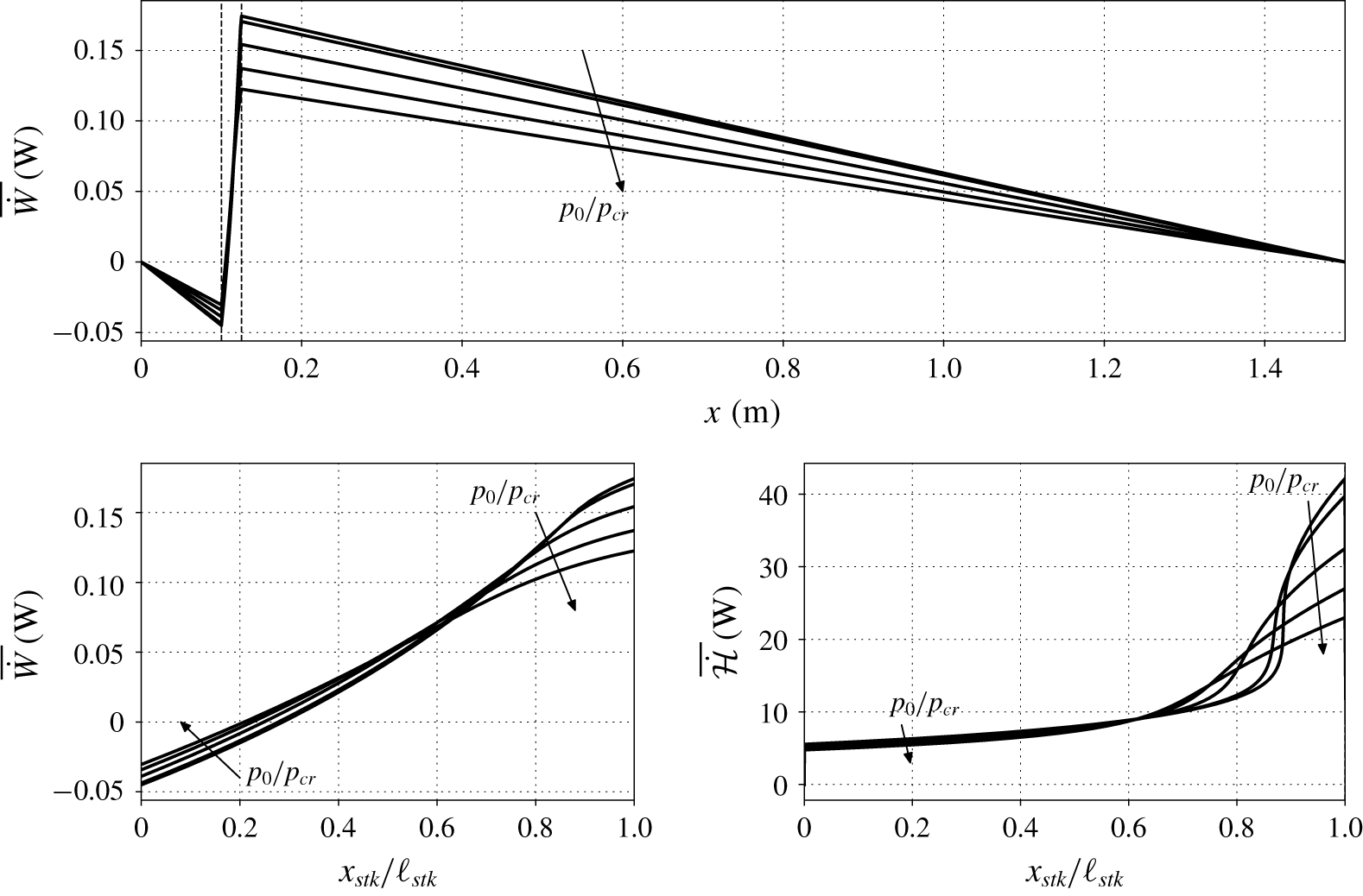
For all values of  $p_{0}$, the acoustic power flows away from the stack, reaching boundary values of zero due the imposed hard wall boundary conditions at both ends of the device (figure 14a), while inside the stack (figure 14b) a positive gradient (see figure 13d) confirms acoustic power production. The trends of the acoustic power inside the stack confirm the intuitive conclusion, drawn from figure 12, that near-critical base pressures entail higher power production in the linear regime. However, the heat input required for sustaining the same pressure oscillations at values of
 $p_{0}$ closer to
 $p_{cr}$ is expected to be higher, given the spike in thermal capacities typical of transcritical conditions.
(a) Acoustic power (4.5) in the whole domain; (b) acoustic power in the stack; (c) total energy flux (4.19) in the stack. Data are taken from the linear stability theory, for  $\unicode[STIX]{x0394}T=100~\text{K}$ and all base pressures of table 2. The values on the
 $y$ axis correspond to a maximum pressure oscillation amplitude of 100 kPa, fixed for all base pressures.

4.2 Total energy budgets
The evolution equation for total energy in two dimensions reads
 $$\begin{eqnarray}\displaystyle \frac{\unicode[STIX]{x2202}\unicode[STIX]{x1D70C}E}{\unicode[STIX]{x2202}t}+\frac{\unicode[STIX]{x2202}\unicode[STIX]{x1D70C}Hu}{\unicode[STIX]{x2202}x}+\frac{\unicode[STIX]{x2202}\unicode[STIX]{x1D70C}Hv}{\unicode[STIX]{x2202}y}=\frac{\unicode[STIX]{x2202}u_{i}\unicode[STIX]{x1D70F}_{i1}}{\unicode[STIX]{x2202}x}+\frac{\unicode[STIX]{x2202}u_{i}\unicode[STIX]{x1D70F}_{i2}}{\unicode[STIX]{x2202}y}-\frac{\unicode[STIX]{x2202}q_{1}}{\unicode[STIX]{x2202}x}-\frac{\unicode[STIX]{x2202}q_{2}}{\unicode[STIX]{x2202}y}, & & \displaystyle\end{eqnarray}$$
where  $E=e+(u^{2}+v^{2})/2$ is the specific total energy, sum of specific internal energy and specific kinetic energy,
 $H=E+p/\unicode[STIX]{x1D70C}$ is the specific total enthalpy, and the other quantities are the same as in (2.7). Integrating (4.11) across the stack pore area, for a two-dimensional rectilinear geometry, yields
 $$\begin{eqnarray}\displaystyle \frac{\unicode[STIX]{x2202}}{\unicode[STIX]{x2202}t}\int _{-h/2}^{h/2}\unicode[STIX]{x1D70C}E\,\text{d}y+\frac{\unicode[STIX]{x2202}}{\unicode[STIX]{x2202}x}\int _{-h/2}^{h/2}\unicode[STIX]{x1D70C}Hu\,\text{d}y=\int _{-h/2}^{h/2}\frac{\unicode[STIX]{x2202}u_{i}\unicode[STIX]{x1D70F}_{i1}}{\unicode[STIX]{x2202}x}\,\text{d}y-\frac{\unicode[STIX]{x2202}}{\unicode[STIX]{x2202}x}\int _{-h/2}^{h/2}q_{1}\,\text{d}y-[q_{2}]_{-h/2}^{h/2},\quad & & \displaystyle\end{eqnarray}$$
where we accounted for  $u=v=0$ at
 $y=\pm h/2$. Introducing the cycle averaging operator
 $$\begin{eqnarray}\displaystyle \overline{(\cdot )}=\frac{\unicode[STIX]{x1D714}}{2\unicode[STIX]{x03C0}}\int _{0}^{2\unicode[STIX]{x03C0}/\unicode[STIX]{x1D714}}(\cdot )\,\text{d}t, & & \displaystyle\end{eqnarray}$$
where time  $0$ indicates the arbitrary beginning of an acoustic cycle, equation (4.12) becomes
 $$\begin{eqnarray}\displaystyle \int _{-h/2}^{h/2}\frac{[\unicode[STIX]{x1D70C}E]_{0}^{2\unicode[STIX]{x03C0}/\unicode[STIX]{x1D714}}}{2\unicode[STIX]{x03C0}/\unicode[STIX]{x1D714}}\,\text{d}y+\frac{\unicode[STIX]{x2202}}{\unicode[STIX]{x2202}x}\int _{-h/2}^{h/2}(\overline{\unicode[STIX]{x1D70C}Hu}+\overline{q_{1}})\,\text{d}y=\int _{-h/2}^{h/2}\overline{\frac{\unicode[STIX]{x2202}u_{i}\unicode[STIX]{x1D70F}_{i1}}{\unicode[STIX]{x2202}x}}\,\text{d}y-[\overline{q_{2}}]_{-h/2}^{h/2}. & & \displaystyle\end{eqnarray}$$
Scaling arguments provided by Swift (Reference Swift1988) allow us to neglect the energy change due to viscous dissipation, first term on the right-hand side of (4.14), which, neglecting terms of third order, becomes
 $$\begin{eqnarray}\displaystyle -[\overline{q_{2}}]_{-h/2}^{h/2}=\int _{-h/2}^{h/2}\frac{[\unicode[STIX]{x1D70C}E]_{0}^{2\unicode[STIX]{x03C0}/\unicode[STIX]{x1D714}}}{2\unicode[STIX]{x03C0}/\unicode[STIX]{x1D714}}\,\text{d}y+\frac{\unicode[STIX]{x2202}\overline{\dot{{\mathcal{H}}}}}{\unicode[STIX]{x2202}x}, & & \displaystyle\end{eqnarray}$$
where
 $$\begin{eqnarray}\displaystyle \overline{\dot{{\mathcal{H}}}}=\int _{-h/2}^{h/2}\left(\overline{\unicode[STIX]{x1D70C}hu}\,\text{d}y-\overline{k\frac{\unicode[STIX]{x2202}T}{\unicode[STIX]{x2202}x}}\right)\text{d}y & & \displaystyle\end{eqnarray}$$
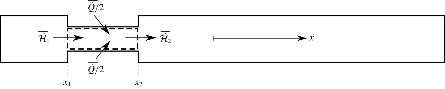
is the fluid’s time-averaged total energy flux. Integrating (4.15) axially along the stack, with  $1$ indicating the axial coordinate of its beginning and
 $2$ its end (see figure 15), yields
 $$\begin{eqnarray}\displaystyle \overline{\dot{Q}}=\int _{x_{1}}^{x_{2}}\int _{-h/2}^{h/2}\frac{[\unicode[STIX]{x1D70C}E]_{0}^{2\unicode[STIX]{x03C0}/\unicode[STIX]{x1D714}}}{2\unicode[STIX]{x03C0}/\unicode[STIX]{x1D714}}\,\text{d}y\,\text{d}x+\overline{\dot{{\mathcal{H}}}}_{2}-\overline{\dot{{\mathcal{H}}}}_{1}, & & \displaystyle\end{eqnarray}$$
where the time-averaged heat exchange through the walls is
 $$\begin{eqnarray}\displaystyle \overline{\dot{Q}}=-\int _{x_{1}}^{x_{2}}[\overline{q_{2}}]_{-h/2}^{h/2}\,\text{d}x=2\int _{x_{1}}^{x_{2}}\overline{\left(k\frac{\unicode[STIX]{x2202}T}{\unicode[STIX]{x2202}y}\right)}_{h/2}\,\text{d}x, & & \displaystyle\end{eqnarray}$$
where we assumed a symmetric temperature profile around  $y=0$. Equation (4.17) shows that the boundary heat flux is absorbed by the fluid in the form of time-averaged total energy flux difference between the two stack extremities.
Control volume (thick dashed lines) used for the total energy balance inside the stack pore in the minimal unit set-up described by figure 3.

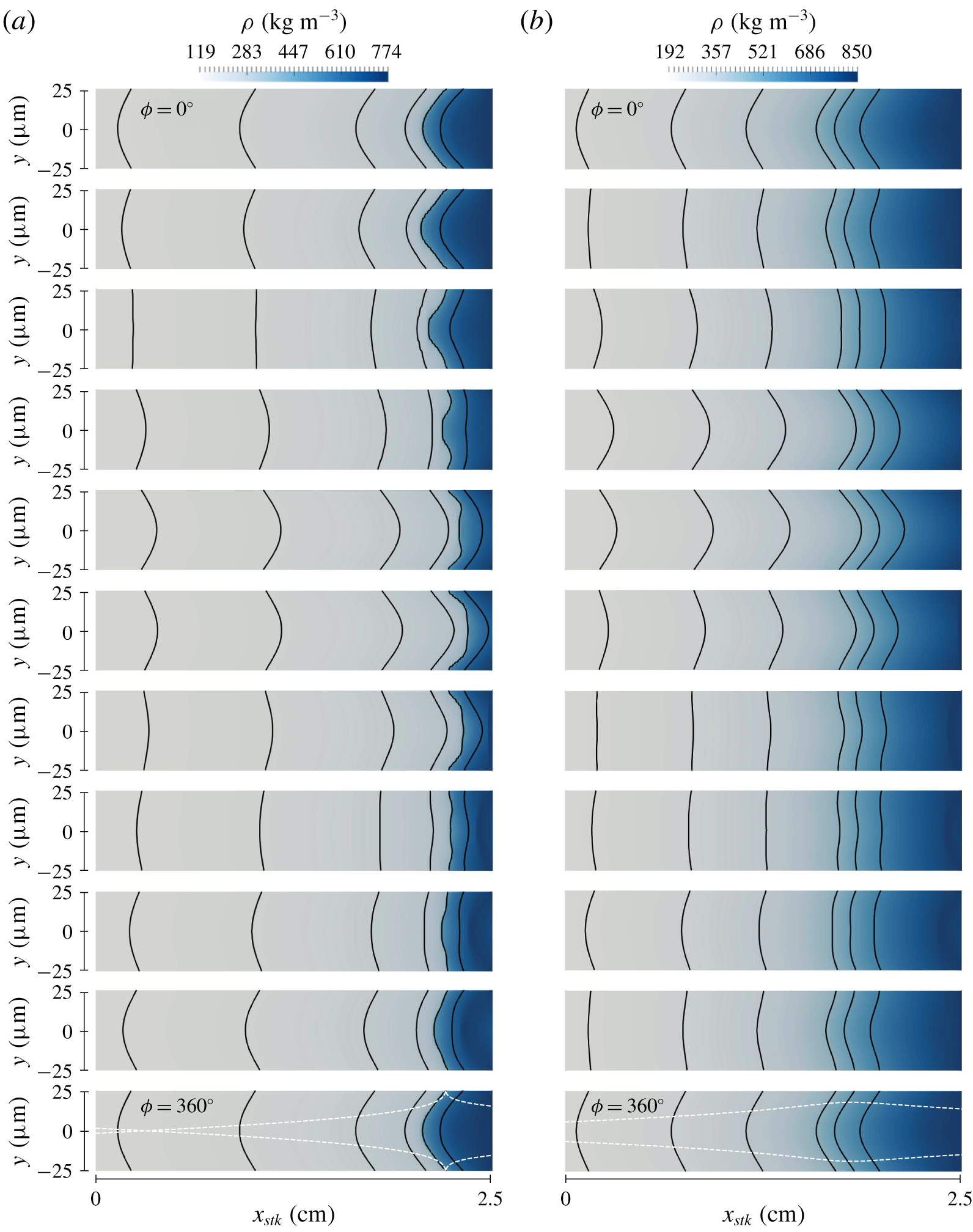
Colour contours of density inside the stack for  $\unicode[STIX]{x0394}T=100~\text{K}$, for
 $p_{0}/p_{cr}=1.01$ (a) and
 $p_{0}/p_{cr}=1.5$ (b) (see table 2), employing grid B with
 $N=3$ (see table 4). A complete acoustic cycle is displayed top to bottom. The results are mirrored about the centre line and stretched 100 times along the
 $y$ axis for plotting purposes. Solid lines indicate isocontours of density for
 $\unicode[STIX]{x1D70C}=125,150,200,260,446.671,650~\text{kg}~\text{m}^{-3}$ (a) and
 $\unicode[STIX]{x1D70C}=200,240,300,450,521.197,620~\text{kg}~\text{m}^{-3}$ (b), while dashed white lines display the local
 $\unicode[STIX]{x1D6FF}_{k}$ (see (5.1)). The density oscillations shown correspond to pressure oscillations of approximately
 $1\,\%$ of the base pressure for both (a) and (b).

The frequency domain expression for the time-averaged energy flux (4.16) is (Swift Reference Swift1988; Ward, Clark & Swift Reference Ward, Clark and Swift2012),
 $$\begin{eqnarray}\overline{\dot{{\mathcal{H}}}}=\frac{1}{2}\text{Re}\left\{\hat{p}\hat{U} ^{\ast }\left(1-\frac{\unicode[STIX]{x1D6FC}_{p_{0}}T_{0}(f_{k}-f_{\unicode[STIX]{x1D708}}^{\ast })}{(1+Pr_{0})(1-f_{\unicode[STIX]{x1D708}}^{\ast })}\right)\right\}+\frac{\unicode[STIX]{x1D70C}_{0}a_{0}^{2}\unicode[STIX]{x1D6E9}|\hat{U} |^{2}}{2AG_{0}\unicode[STIX]{x1D714}|1-f_{\unicode[STIX]{x1D708}}|^{2}}\text{Im}\left\{\frac{f_{\unicode[STIX]{x1D708}}^{\ast }Pr_{0}+f_{k}}{1-Pr_{0}^{2}}\right\}+H_{k},\end{eqnarray}$$
where
 $$\begin{eqnarray}\displaystyle H_{k}=-Ak_{0}\frac{\text{d}T_{0}}{\text{d}x} & & \displaystyle\end{eqnarray}$$
is the conductive axial heat flux, and where
 $$\begin{eqnarray}\displaystyle G=\frac{\unicode[STIX]{x1D6FC}_{p}a^{2}}{c_{p}}=\frac{\unicode[STIX]{x1D6FE}-1}{\unicode[STIX]{x1D6FC}_{p}T}, & & \displaystyle\end{eqnarray}$$
is the Grüneisen parameter, which reverts to  $\unicode[STIX]{x1D6FE}-1$ for ideal gases, and which is described by Swift et al. (Reference Swift, Migliori, Hofler and Wheatley1985) as the ratio between the work parameter
 $\unicode[STIX]{x1D6FE}-1$ and the heat parameter
 $\unicode[STIX]{x1D6FC}_{p}T$. For our configuration,
 $\overline{\dot{{\mathcal{H}}}}$ is equal to the acoustic power when computed outside of the stack.
The profile of  $\overline{\dot{{\mathcal{H}}}}$ inside the stack (figure 14c) shows the cumulative time-averaged heat in Watts required from the solid walls of the stack to sustain the fluid oscillations (ignoring the first term on the right-hand side of (4.17)). The axial derivative of
 $\overline{\dot{{\mathcal{H}}}}$ represents the pointwise heat per unit length (
 $\text{W}~\text{m}^{-1}$) injected into the fluid. The highest wall heat flux is required to sustain carbon dioxide oscillating around its PB state, followed by fluid in PL and PG conditions, on its right and left, respectively, which is a hierarchy consistent with the one of the isobaric specific heat capacities of each thermodynamic condition. For a given
 $\unicode[STIX]{x0394}T$, conditions closer to the critical point do produce more acoustic power, but also require more energy to be sustained.
The efficiency of the thermal-to-acoustic energy transformation can be computed by dividing the produced acoustic power to the total energy required by the stack,
 $$\begin{eqnarray}\displaystyle \unicode[STIX]{x1D702}=\frac{\overline{{\dot{W}}}_{2}-\overline{{\dot{W}}}_{1}}{\overline{\dot{Q}}}. & & \displaystyle\end{eqnarray}$$
This estimate can be more accurately performed if a limit cycle is present (to cancel the unsteady term in (4.17)). In order to do so, nonlinear effects need to be considered, as done in the remainder of the manuscript.
5 Thermodynamic nonlinearities at moderate pressure amplitudes
For moderate pressure amplitude values (of approximately  $1\,\%\,p_{0}$), rapid, asymmetric and strong density oscillations are observed for
 $p_{0}/p_{cr}=1.01$ (figure 16a), close to the right-hand side of the stack, where PB conditions allow large variations of thermodynamic properties from small temperature perturbations. At the beginning of the acoustic cycle, the PB density contour (
 $\unicode[STIX]{x1D70C}=446.671~\text{kg}~\text{m}^{-3}$) is skewed towards the left, where fluid in PG conditions is present, while it does not extend as much towards the right, halfway through the acoustic cycle, where the PL fluid is. Moreover, the phasing between PG density oscillations (
 $\unicode[STIX]{x1D70C}=260~\text{kg}~\text{m}^{-3}$) and PL ones (
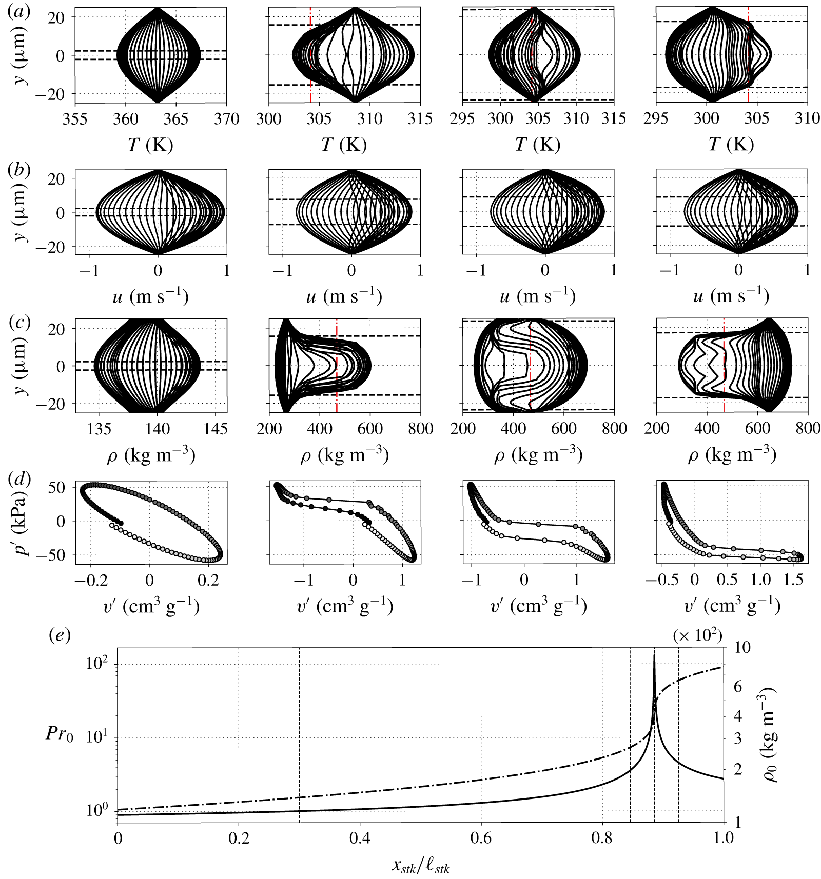
 $\unicode[STIX]{x1D70C}=650~\text{kg}~\text{m}^{-3}$) is similar, whereas the PB fluid lags behind, especially in the centre of the channel. In fact, when critical conditions are achieved near the centre of the pore, the thermodynamic properties show a rather flat transverse distribution (figure 17a,c), due to the high spike in thermal capacity. The thermal inertia is responsible for the increased residence time of the fluid around PB conditions, and contributes to its nonlinear time phasing difference with respect to the oscillations of PG and PL fluid.
Time evolution, during the transient phase, of cross-sectional profiles of temperature (a), axial velocity (b), and density (c) inside the stack, with resulting Lagrangian pressure–volume cycle at the centre line (d), for  $\unicode[STIX]{x0394}T=100~\text{K}$ and
 $p_{0}/p_{cr}=1.01$ (see table 1), for grid B with
 $N=3$ (see table 4). Darker to lighter coloured circles indicate increasing time in (d), which considers a complete acoustic period. The results in (a), (b), and (c), for plotting purposes, are mirrored about the centre line, and are considered until 70 % of the acoustic cycle completion. Horizontal dashed lines indicate the distance from the walls equal to
 $\unicode[STIX]{x1D6FF}_{k}$ in (a) and (c), and to
 $\unicode[STIX]{x1D6FF}_{\unicode[STIX]{x1D708}}$ in (b), and vertical dashed-dotted lines are plotted for
 $T=T_{cr}$ in (a) and for
 $\unicode[STIX]{x1D70C}=\unicode[STIX]{x1D70C}_{cr}$ in (c). Panel (e) shows the base density (dashed-dotted line) and the base Prandtl number (solid line), and vertical dashed lines at
 $x=10.75~\text{cm},12.11~\text{cm},12.21~\text{cm},12.31~\text{cm}$, which are the axial coordinates from where the
 $y$-profiles in (a), (b), (c) are extracted from, and the initial locations for the acoustic parcel in (d). For this case, the strength of the initial perturbation is
 $p_{amp}=5\times 10^{-3}$ (see (2.9)).

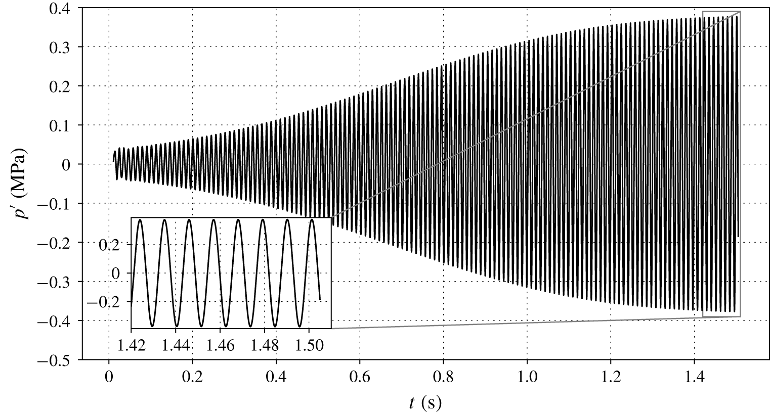
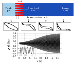
Pressure fluctuations detected by a probe at  $x=L$ and
 $y=0$, for
 $\unicode[STIX]{x0394}T=30~\text{K}$ and
 $p_{0}=1.01p_{cr}$, from Navier–Stokes simulations with grid A and
 $N=2$.

On the other hand, for  $p_{0}/p_{cr}=1.5$ (figure 16b), which is sufficiently far from the critical pressure, the stability dynamics is more akin to the ones of ideal gases: away from strong base density gradients, the fluid in the stack undergoes mild and symmetric density oscillations, all with approximately the same relative phasing. Moreover, the acoustic time scale is comparable to the time of thermal diffusion in the
 $y$ direction, hence allowing for harmonic density perturbations in all the stack.
In fact, the peculiar behaviour of transcritical fluids is connected to the axial profiles of the viscous and thermal boundary layers thicknesses  $\unicode[STIX]{x1D6FF}_{\unicode[STIX]{x1D708}},\unicode[STIX]{x1D6FF}_{k}$, defined by
 $$\begin{eqnarray}\displaystyle \unicode[STIX]{x1D6FF}_{\unicode[STIX]{x1D708}}^{2}=\frac{2\unicode[STIX]{x1D708}_{0}}{\unicode[STIX]{x1D714}},\quad \unicode[STIX]{x1D6FF}_{k}^{2}=\frac{2k_{0}}{\unicode[STIX]{x1D714}\unicode[STIX]{x1D70C}_{0}c_{p_{0}}}=\frac{\unicode[STIX]{x1D6FF}_{\unicode[STIX]{x1D708}}^{2}}{Pr_{0}}. & & \displaystyle\end{eqnarray}$$
Since the viscous boundary layer thickness, even for  $p_{0}/p_{cr}=1.01$, covers most of the fluid inside the stack in all its regions, the cross-sectional velocity profiles resemble their linear counterparts (predicted by the theory of Rott), and do not show significant changes among the different fluid conditions (figure 17b). Real-fluid effects are mainly manifest in the oscillating thermodynamic variables, such as density and temperature, but not in the velocity. Indeed, while for gases the Prandtl number is commonly less than unity, and for liquids usually
 $Pr>1$, in the PB region the Prandtl number can reach values of 100 (see figure 13a). This leads to such a low ratio of thermal boundary layer thickness to half-height of the pore,
 $\unicode[STIX]{x1D6FF}_{k}/r$, that most of the fluid in the pore cannot be heated or cooled by the walls during an acoustic cycle (bottom of figure 16a). Therefore, fluid in PB conditions is thermally shielded, and shows large variations and asymmetric characteristics in the transverse profiles of density (figure 17c).
The fluid ejection around PB conditions confirms the presence of convective nonlinearities, and suggests that the modal assumption of linear fluctuations is locally violated due to the large changes in particle volume. Indeed, as a result of the PB thermodynamics, the linear relation between density and temperature (A 22), which holds for small wave amplitudes, is replaced by a fully nonlinear relationship even at moderate pressure amplitudes, resulting in a distortion of the Lagrangian pressure–volume cycle (figure 17d). However, away from the PB region (and also for higher values of  $p_{0}$ away from
 $p_{cr}$), a
 $pv$ cycle typical of the linear regime (figure 12) is observed (plot on the left of figure 17d). Moreover, pressure oscillation amplitudes, for all values of
 $p_{0}/p_{cr}$, still grow at approximately the rate predicted by the linear theory even with the presence of the aforementioned convective nonlinearities.
In summary, oscillations of transcritical fluids with  $p_{0}/p_{cr}\simeq 1$ present a nonlinear behaviour localized in the small region of the stack where PB conditions are present. However, as discussed in the following section, these nonlinearities are not the ones governing the system’s limit cycle.
6 Limit cycle due to minor area losses
A limit cycle can be achieved if pressure amplitudes are sufficiently high to trigger nonlinear losses, balancing acoustic energy production via a nonlinear dissipation term, resulting in a zero net energy growth (see (4.3)). One mechanism that can provide high enough nonlinear losses for a limit cycle in a minimal unit calculation is the formation of shock waves (Gupta et al. Reference Gupta, Lodato and Scalo2017). However, pressurized liquids can sustain large pressure wave amplitudes without the generation of higher harmonics or shock waves. In fact, the pressure amplitude above which acoustic nonlinearities occur,  $|p|_{nl}$, which is approximately equal to the reference pressure
 $\unicode[STIX]{x1D70C}_{0}a_{0}^{2}$ (Migliorino & Scalo Reference Migliorino and Scalo2017), is of the order of hundreds of MPa, corresponding to approximately 15 times the base pressure (table 5), whereas values around 1 %–2 % of
 $p_{0}$ are usually expected for ideal gases. Indeed, Swift (Reference Swift1992) reported the formation of higher harmonics (which indicate incumbent wave steeping) in his experiments on a large-scale ideal-gas thermoacoustic engine, with pressure amplitudes of 10 % of the base pressure, and Gupta et al. (Reference Gupta, Lodato and Scalo2017) showed shock waves at 7 % of the base pressure in their numerical travelling wave set-up with an ideal gas. On the other hand, Migliori & Swift (Reference Migliori and Swift1988) did not report any trace of higher harmonics at
 $|p|_{max}/p_{0}=55\,\%$ in their liquid sodium thermoacoustic device, and even proposed a future design for which
 $|p|_{max}/p_{0}=100\,\%$. The Navier–Stokes simulations carried out in this study from the linear regime to the limit cycle confirm that pressure traces are harmonic (figure 18). A minimal-unit set-up such as the current one will require more acoustic periods to obtain a limit cycle than full scale devices, such as the one investigated by Lin et al. (Reference Lin, Scalo and Hesselink2016), due to its reduced thermoviscous losses. As done in previous studies by Scalo et al. (Reference Scalo, Lele and Hesselink2015), Lin et al. (Reference Lin, Scalo and Hesselink2016) and Gupta et al. (Reference Gupta, Lodato and Scalo2017) a limit cycle is achieved by simulating the complete transient evolution of the system, comprising modal growth and nonlinear saturation, on a coarse grid first. Upon reaching a limit cycle on such grid, the solution is interpolated on progressively finer grids until adequate resolution is reached. On the other hand, when analysing the grid sensitivity analysis of growth rates extracted from the Navier–Stokes simulations, as done in figure 6, all available grid resolutions are adopted from the beginning, and simulations are halted after approximately 8–30 cycles. In no case the complete evolution of the system, from initial conditions to a limit cycle, is simulated on the finest grid available, nor it is advisable to do so.
In the computational set-up considered in this study, the main source of nonlinear dissipation is the vortex shedding at locations of sudden area change, which are the transition from the hot cavity to the stack and from the latter to the duct on its right (see figure 3). Such area jumps entail pressure drops, or minor losses, which can be parametrized as (Idelchik Reference Idelchik2003; Lin et al. Reference Lin, Scalo and Hesselink2016)
 $$\begin{eqnarray}\displaystyle \unicode[STIX]{x0394}\hat{p}_{ml}=-\frac{K}{2}\unicode[STIX]{x1D70C}_{0}\frac{\hat{U} |\hat{U} |_{lc}}{A_{0}^{2}}, & & \displaystyle\end{eqnarray}$$
where  $|\hat{U} |/A_{0}$ is the largest average velocity in the channel and
 $K$ is defined by
 $$\begin{eqnarray}\displaystyle K=K_{exp}(A_{0}/A_{1},Re)+K_{contr}(A_{0}/A_{1},Re), & & \displaystyle\end{eqnarray}$$
where  $A_{0}$ is the smaller and
 $A_{1}$ the larger area. Equation (6.2) considers losses in steady flow due to expansions together with losses from contractions, both dependent, as indicated in Idelchik (Reference Idelchik2003), on the Reynolds number
 $$\begin{eqnarray}\displaystyle Re=\frac{\unicode[STIX]{x1D70C}_{0}h|\hat{U} |_{lc}/A_{0}}{\unicode[STIX]{x1D707}_{0}}, & & \displaystyle\end{eqnarray}$$
where  $h$ is the height of the stack (see figure 3). The values of
 $|\hat{U} |$ at limit cycle,
 $|\hat{U} |_{lc}$, which are different for each area jump, are computed iteratively until a zero growth rate is obtained from the numerical solution of (2.10a) and (2.10b).
Base pressure, base density times square of base speed of sound, equal to the approximate pressure amplitude limit for nonlinear wave propagation,  $|p|_{nl}$, and ratio of
 $|p|_{nl}$ over base pressure. Data are for all the base pressures of table 2 and for
 $T=293.15~\text{K}$.

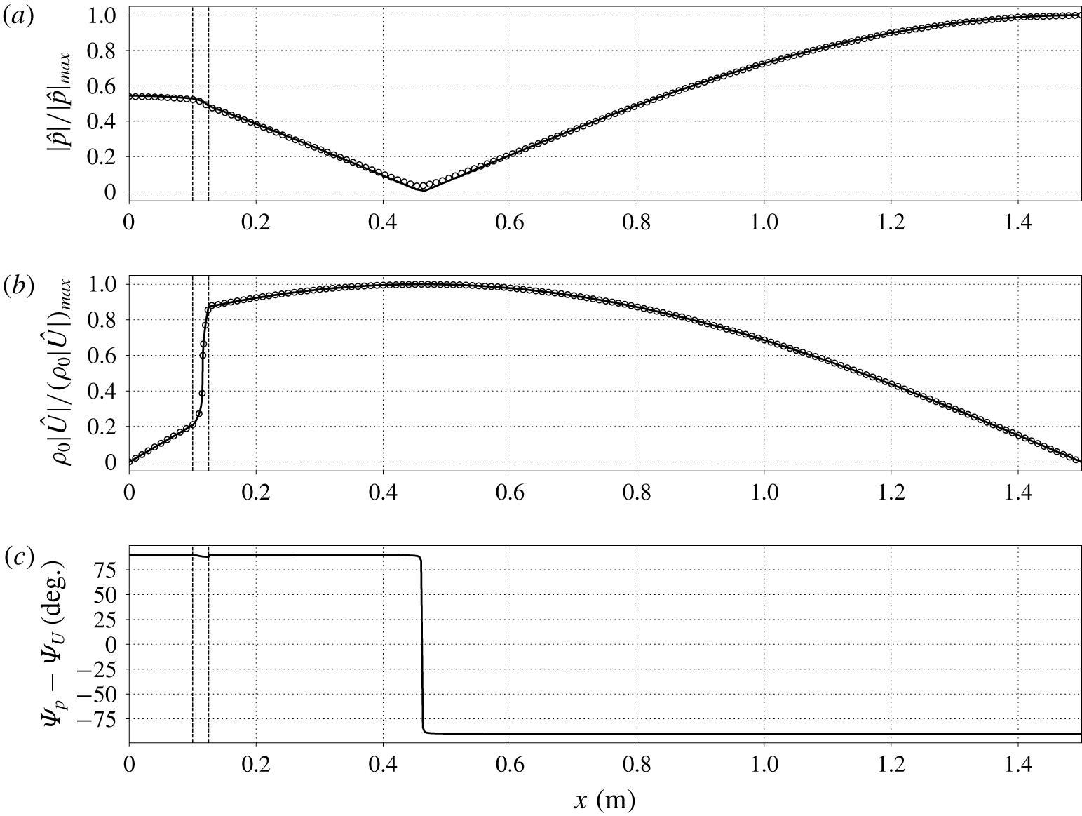
Axial distribution of pressure (a) and mass flow rate (b) dimensionless amplitudes, and phasing between  $\hat{p}$ and
 $\hat{U}$ (c), for
 $\unicode[STIX]{x0394}T=30~\text{K}$ and
 $p_{0}=1.01p_{cr}$, for grid A with
 $N=3$ (see table 4), at limit cycle: linear theory augmented with linearized minor losses (solid lines), data extracted from the Navier–Stokes simulations (circles). Vertical dashed lines indicate locations of abrupt area change.

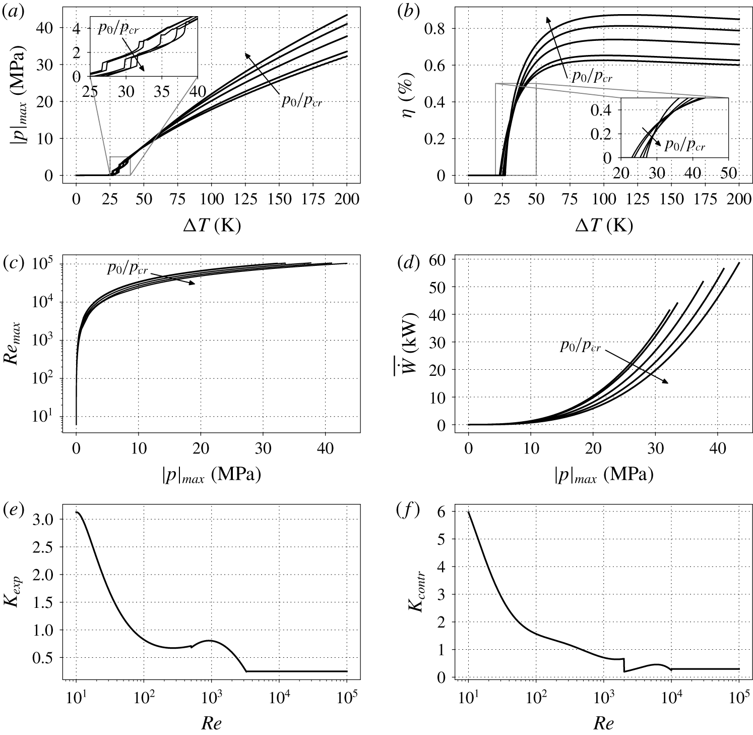
Data on limit cycle achieved due to linearized area losses (6.1) for all base pressures of table 2: (a) maximum pressure amplitude; (b) thermal-to-acoustic efficiency (4.22); (c) Reynolds number (6.3); (d) acoustic power produced by the stack; (e,f)  $K_{exp},K_{contr}$ appearing in (6.2) versus Reynolds number for
 $A_{0}/A_{1}=0.5$ (Idelchik Reference Idelchik2003).

The linear stability theory augmented with linearized minor losses is able to correctly reproduce the axial profiles obtained from the fully nonlinear Navier–Stokes simulations (figure 19a,b), as was also shown by Lin et al. (Reference Lin, Scalo and Hesselink2016). With respect to the linear regime, (figure 9), the pressure amplitude minimum is null (since  $\unicode[STIX]{x1D6FC}/\unicode[STIX]{x1D714}=0$ at limit cycle) and the mass flow rate inside the stack varies more steeply at PB conditions, but the overall axial profiles of pressure amplitude and mass flow rate do not vary considerably. Instead, at limit cycle, the phasing between pressure and flow rate is uniform in the entire resonator, apart from a sharp variation from
 $90^{\circ }$ to
 $-90^{\circ }$ (figure 19c).
Equations (6.1) and (6.2), by taking into account transitional and fully developed turbulence, are necessary for the quantitative prediction of realistic limit cycle thermoacoustic oscillations (figure 20), which is not obtainable with the two-dimensional Navier–Stokes simulations.
Pressure amplitudes are the highest for near-critical conditions only for values of  $\unicode[STIX]{x0394}T$ below 50 K (figure 20a). Furthermore, for a fixed pressure amplitude, conditions away from the critical point are characterized by the lowest Reynolds numbers (figure 20c) and work output (figure 20d), consistent with that observed in the linear regime (§ 4.1). Thus, as also pointed out by Swift (Reference Swift1988), higher power energy densities are achieved by fluids with larger thermal expansion coefficients, such as fluids with
 $p_{0}/p_{cr}\simeq 1$. However, the efficiency of thermal to acoustic energy conversion is the highest for base pressures closer to the critical pressure only if
 $\unicode[STIX]{x0394}T<30~\text{K}$ (figure 20b), consistent with the theoretical findings of Swift (Reference Swift1988), where higher acoustic powers were associated with lower efficiencies. The maximum efficiency observed is
 $\unicode[STIX]{x1D702}=0.87\,\%$, obtained for
 $p_{0}/p_{cr}=1.5$ and
 $\unicode[STIX]{x0394}T=119~\text{K}$. For the sake of comparison, Migliori & Swift (Reference Migliori and Swift1988), with their liquid sodium thermoacoustic engine, obtained 18 W of acoustic power, employing a 360 K temperature difference across the stack with 990 W of required heat, for an efficiency of 1.8 %. Notice that the computational set-up used in this work was not originally optimized for thermal-to-acoustic efficiency, but for growth rate instead (see § 2.2.2).
The nonlinear behaviour exhibited by the pressure amplitude trends for  $\unicode[STIX]{x0394}T<40~\text{K}$ (see inset in figure 20a), which correspond to Reynolds numbers below
 $10^{4}$, are due to the trends of
 $K_{exp}$ and
 $K_{contr}$ appearing in (6.2) (figure 20e,f). For large Reynolds numbers, equation (6.2) becomes (Idelchik Reference Idelchik2003)
 $$\begin{eqnarray}\displaystyle K_{exp}=\left(1-\frac{A_{0}}{A_{1}}\right)^{2}\quad \text{for }Re>3.3\times 10^{3},\quad K_{contr}=\frac{1}{2}\left(1-\frac{A_{0}}{A_{1}}\right)^{3/4}\quad \text{for }Re>10^{4}, & & \displaystyle \nonumber\\ \displaystyle & & \displaystyle\end{eqnarray}$$
where the first expression is the Borda–Carnot formula. For more accurate predictions of the limit cycle physics, it is recommended that an accurate parametrization for  $K$, i.e. accounting for oscillatory flow, is obtained.
7 Conclusions
This work has unveiled the fundamental physics of transcritical thermoacoustics through the first direct numerical simulation of a thermoacoustically unstable resonator employing carbon dioxide in transcritical conditions. The main takeaways of this manuscript are the strong real-fluid effects observed in the linear and nonlinear regimes, which are, more specifically as follows:
(i) The high value of the growth rate to frequency ratio (
 $\unicode[STIX]{x1D6FC}/\unicode[STIX]{x1D714}$) which requires, unlike the ideal gas cases, the thermoviscous functions in the linear theory formulation to be based on the fully complex eigenvalue $\unicode[STIX]{x1D6FC}+\text{i}\unicode[STIX]{x1D714}$, rather than just its imaginary part $\unicode[STIX]{x1D714}$.
(ii) When the fluid inside the stack approaches pseudo-boiling conditions, the frequency of oscillations drops steeply with small changes in
$\unicode[STIX]{x0394}T$, with the growth rate exhibiting a non-monotonic dependency with respect to the base pressure $p_{0}$.(iii) A more prominent travelling-wave component than that found in ideal-gas systems in similar configurations is observed at the location of minimum pressure amplitude.
(iv) Due to the steeply varying acoustic impedance, pressure, mass flow rate, and acoustic power exhibit a discontinuity in their first spatial derivative at pseudo-boiling conditions.
(v) The acoustic energy budgets indicate a boost in thermoacoustic production at transcritical conditions, together with a sharp increase in thermoacoustic dissipation; also, the profiles of acoustic power and total energy flux inside the stack suggest that conditions closer to the critical point produce additional power but require more heat input to be sustained.
(vi) Moderate pressure amplitude values (of approximately
$1\,\%\,p_{0}$) trigger thermodynamic nonlinearities, resulting in a highly distorted pressure–volume work cycle, due to the gradients in the base state profiles typical of transcritical fluids with $p_{0}\simeq p_{cr}$. However, these nonlinearities are found to be localized in a small region of the stack, and are not responsible for regulating the limit cycle, which is dominated by minor losses at the area jump locations. Axial profiles obtained from the Navier–Stokes simulations pushed to limit cycle are well reproduced by the linear stability theory augmented with linearized minor losses. For this standing-wave configuration, a prediction of the maximum efficiency of thermal to acoustic energy conversion is 0.87 % at $p_{0}/p_{cr}=1.5$ and $\unicode[STIX]{x0394}T=119~\text{K}$. Limit cycle work output is found to be always higher for near-critical conditions.


The findings of this work could be helpful for future theoretical and experimental studies on transcritical thermoacoustic instabilities. Future work needs to consider three-dimensional Navier–Stokes simulations for the accurate prediction of the limit cycle physics. Such investigation could shed light on the modelling strategy needed for the pressure drop located at abrupt area jumps, and on the importance of the convective nonlinearities occurring around transcritical conditions. In addition, the effect of bulk viscosity and of gravity needs to be assessed. Moreover, linear stability tools able to consider the steady state energy balance in the stack, with companion conjugate heat transfer Navier–Stokes simulations, need to be considered in the case of transcritical fluids. Finally, more realistic geometrical configurations, such as geometries comprising more than one minimal unit, are desirable.
Acknowledgements
M.T.M. acknowledges the support of the F. N. Andrews and Rolls-Royce Doctoral Fellowships at Purdue University. The use of the SD solver originally developed by Antony Jameson’s group at Stanford University is gratefully acknowledged. The computing resources were provided by the Rosen Center for Advanced Computing (RCAC) at Purdue University and Information Technology at Purdue (ITaP). This work was performed under financial support of the Rolls-Royce University Technology Center at Purdue University, grant number 8000-00198451.
Appendix A. Derivation of the harmonic equations
The evolution equations for mass, axial momentum, and pressure ((2.5), (2.6) and (2.7), respectively), in a two-dimensional domain, with  $x$ (
 $j=1$) corresponding to the axial direction and
 $r$ (
 $j=2$) to the radial direction, read
 $$\begin{eqnarray}\displaystyle & \displaystyle \frac{\unicode[STIX]{x2202}\unicode[STIX]{x1D70C}}{\unicode[STIX]{x2202}t}+u_{j}\frac{\unicode[STIX]{x2202}\unicode[STIX]{x1D70C}}{\unicode[STIX]{x2202}x_{j}}=-\unicode[STIX]{x1D70C}\left(\frac{\unicode[STIX]{x2202}u}{\unicode[STIX]{x2202}x}+\frac{1}{r^{m}}\frac{\unicode[STIX]{x2202}r^{m}v}{\unicode[STIX]{x2202}r}\right), & \displaystyle\end{eqnarray}$$
 $$\begin{eqnarray}\displaystyle & \displaystyle \unicode[STIX]{x1D70C}\left(\frac{\unicode[STIX]{x2202}u}{\unicode[STIX]{x2202}t}+u_{j}\frac{\unicode[STIX]{x2202}u}{\unicode[STIX]{x2202}x_{j}}\right)=-\frac{\unicode[STIX]{x2202}p}{\unicode[STIX]{x2202}x}+\frac{\unicode[STIX]{x1D707}}{r^{m}}\frac{\unicode[STIX]{x2202}}{\unicode[STIX]{x2202}r}\left(r^{m}\frac{\unicode[STIX]{x2202}u}{\unicode[STIX]{x2202}r}\right), & \displaystyle\end{eqnarray}$$
 $$\begin{eqnarray}\displaystyle & \displaystyle \frac{\unicode[STIX]{x2202}p}{\unicode[STIX]{x2202}t}+u\frac{\unicode[STIX]{x2202}p}{\unicode[STIX]{x2202}x}=a^{2}\left(\frac{\unicode[STIX]{x2202}\unicode[STIX]{x1D70C}}{\unicode[STIX]{x2202}t}+u_{j}\frac{\unicode[STIX]{x2202}\unicode[STIX]{x1D70C}}{\unicode[STIX]{x2202}x_{j}}\right)+\frac{\unicode[STIX]{x1D6FC}_{p}a^{2}}{c_{p}}\left(\unicode[STIX]{x1D70F}_{ij}\frac{\unicode[STIX]{x2202}u_{i}}{\unicode[STIX]{x2202}x_{j}}+\frac{k}{r^{m}}\frac{\unicode[STIX]{x2202}}{\unicode[STIX]{x2202}r}\left(r^{m}\frac{\unicode[STIX]{x2202}T}{\unicode[STIX]{x2202}r}\right)\right), & \displaystyle\end{eqnarray}$$
where we considered Cartesian ( $m=0$) or cylindrical (
 $m=1$) coordinates, neglected axial viscous and conduction stresses, assumed that
 $\unicode[STIX]{x1D707}=\unicode[STIX]{x1D707}(x)$ and
 $k=k(x)$, and disregarded the momentum equation in the
 $r$ direction (
 $\unicode[STIX]{x2202}p/\unicode[STIX]{x2202}r=0$,
 $v=v(r)$ and negligible viscous stresses along
 $r$).
A first-order Taylor expansion is assumed, both for thermodynamic and kinematic variables,
 $$\begin{eqnarray}\displaystyle \left.\begin{array}{@{}c@{}}\unicode[STIX]{x1D70C}=\unicode[STIX]{x1D70C}_{0}(x)+\unicode[STIX]{x1D70C}^{\prime }(x,y,t),\quad T=T_{0}(x)+T^{\prime }(x,y,t),\quad p=p_{0}+p^{\prime }(x,t),\\ u=u^{\prime }(x,y,t),\quad v=v^{\prime }(y),\end{array}\right\} & & \displaystyle\end{eqnarray}$$
where a generic variable is composed of a base quantity, at most varying axially, a fluctuation that is time and space dependent, and no mean flow is considered. Neglecting nonlinear terms, and with the assumptions in (A 4), equation (A 2) becomes
 $$\begin{eqnarray}\displaystyle & \displaystyle \frac{\unicode[STIX]{x2202}\unicode[STIX]{x1D70C}^{\prime }}{\unicode[STIX]{x2202}t}+u^{\prime }\frac{\text{d}\unicode[STIX]{x1D70C}_{0}}{\text{d}x}=-\unicode[STIX]{x1D70C}_{0}\left(\frac{\unicode[STIX]{x2202}u^{\prime }}{\unicode[STIX]{x2202}x}+\frac{1}{r^{m}}\frac{\unicode[STIX]{x2202}r^{m}v^{\prime }}{\unicode[STIX]{x2202}r}\right), & \displaystyle\end{eqnarray}$$
 $$\begin{eqnarray}\displaystyle & \displaystyle \unicode[STIX]{x1D70C}_{0}\frac{\unicode[STIX]{x2202}u^{\prime }}{\unicode[STIX]{x2202}t}=-\frac{\unicode[STIX]{x2202}p^{\prime }}{\unicode[STIX]{x2202}x}+\frac{\unicode[STIX]{x1D707}_{0}}{r^{m}}\frac{\unicode[STIX]{x2202}}{\unicode[STIX]{x2202}r}\left(r^{m}\frac{\unicode[STIX]{x2202}u^{\prime }}{\unicode[STIX]{x2202}r}\right), & \displaystyle\end{eqnarray}$$
 $$\begin{eqnarray}\displaystyle & \displaystyle \frac{\unicode[STIX]{x2202}p^{\prime }}{\unicode[STIX]{x2202}t}=a_{0}^{2}\left(\frac{\unicode[STIX]{x2202}\unicode[STIX]{x1D70C}^{\prime }}{\unicode[STIX]{x2202}t}+u^{\prime }\frac{\text{d}\unicode[STIX]{x1D70C}_{0}}{\text{d}x}\right)+\frac{\unicode[STIX]{x1D6FE}_{0}-1}{\unicode[STIX]{x1D6FC}_{p_{0}}T_{0}}\frac{k_{0}}{r^{m}}\frac{\unicode[STIX]{x2202}}{\unicode[STIX]{x2202}r}\left(r^{m}\frac{\unicode[STIX]{x2202}T^{\prime }}{\unicode[STIX]{x2202}r}\right), & \displaystyle\end{eqnarray}$$
where we used the thermodynamic relation  $a^{2}T\unicode[STIX]{x1D6FC}_{p}^{2}/c_{p}=\unicode[STIX]{x1D6FE}-1$.
Introducing the variables
 $$\begin{eqnarray}\displaystyle U^{\prime }=\int _{-\unicode[STIX]{x1D6FF}_{0m}h/2}^{h/2}u^{\prime }(x,r,t)(2\unicode[STIX]{x03C0}r)^{m}\,\text{d}r,\quad A=\int _{-\unicode[STIX]{x1D6FF}_{0m}h/2}^{h/2}(2\unicode[STIX]{x03C0}r)^{m}\,\text{d}r, & & \displaystyle\end{eqnarray}$$
which are, respectively, the volumetric flow rate fluctuations and the cross-sectional area for cylindrical coordinates  $(m=1)$, or pore height times 1 m for rectilinear coordinates
 $(m=0)$, and integrating (A 6) over the cross-section, we obtain
 $$\begin{eqnarray}\displaystyle \unicode[STIX]{x1D70C}_{0}\frac{\unicode[STIX]{x2202}U^{\prime }}{\unicode[STIX]{x2202}t}=-A\frac{\unicode[STIX]{x2202}p^{\prime }}{\unicode[STIX]{x2202}x}+\unicode[STIX]{x1D70F}_{w}^{\prime },\quad A\frac{\unicode[STIX]{x2202}p^{\prime }}{\unicode[STIX]{x2202}t}=-\unicode[STIX]{x1D70C}_{0}a_{0}^{2}\frac{\unicode[STIX]{x2202}U^{\prime }}{\unicode[STIX]{x2202}x}+\frac{\unicode[STIX]{x1D6FE}_{0}-1}{\unicode[STIX]{x1D6FC}_{p_{0}}T_{0}}q^{\prime }, & & \displaystyle\end{eqnarray}$$
after accounting for impenetrable boundary conditions in  $r$, and assuming symmetry of the fluctuations around the centre line of the duct in the expressions of the wall shear stress and the wall heat flux, respectively,
 $$\begin{eqnarray}\displaystyle \unicode[STIX]{x1D70F}_{w}^{\prime }=2\unicode[STIX]{x1D707}_{0}\left(\frac{\unicode[STIX]{x03C0}h}{2}\right)^{m}\left.\frac{\unicode[STIX]{x2202}u^{\prime }}{\unicode[STIX]{x2202}r}\right|_{r=h/2},\quad q^{\prime }=2k_{0}\left(\frac{\unicode[STIX]{x03C0}h}{2}\right)^{m}\left.\frac{\unicode[STIX]{x2202}T^{\prime }}{\unicode[STIX]{x2202}r}\right|_{r=h/2}. & & \displaystyle\end{eqnarray}$$
Assuming an harmonic dependence of the perturbations (normal mode assumption),
 $$\begin{eqnarray}\displaystyle \left.\begin{array}{@{}c@{}}\unicode[STIX]{x1D70C}^{\prime }=\hat{\unicode[STIX]{x1D70C}}(x,r)\text{e}^{\unicode[STIX]{x1D70E}t},\quad T^{\prime }=\hat{T}(x,r)\text{e}^{\unicode[STIX]{x1D70E}t},\quad p^{\prime }=\hat{p}(x)\text{e}^{\unicode[STIX]{x1D70E}t},\\ u^{\prime }=\hat{u} (x,r)\text{e}^{\unicode[STIX]{x1D70E}t},\quad v^{\prime }=\hat{v}(r)\text{e}^{\unicode[STIX]{x1D70E}t},\end{array}\right\} & & \displaystyle\end{eqnarray}$$
where it is intended that the physical solution of all the perturbations is the real part of the respective expressions, equation (A 6) becomes
 $$\begin{eqnarray}\displaystyle & \displaystyle \unicode[STIX]{x1D70E}\hat{\unicode[STIX]{x1D70C}}=-\unicode[STIX]{x1D70C}_{0}\frac{\unicode[STIX]{x2202}\hat{u} }{\unicode[STIX]{x2202}x}-\hat{u} \frac{\text{d}\unicode[STIX]{x1D70C}_{0}}{\text{d}x}-\frac{\unicode[STIX]{x1D70C}_{0}}{r^{m}}\frac{\unicode[STIX]{x2202}r^{m}\hat{v}}{\unicode[STIX]{x2202}r}, & \displaystyle\end{eqnarray}$$
 $$\begin{eqnarray}\displaystyle & \displaystyle \unicode[STIX]{x1D70E}\hat{u} =-\frac{1}{\unicode[STIX]{x1D70C}_{0}}\frac{\text{d}\hat{p}}{\text{d}x}+\frac{\unicode[STIX]{x1D708}_{0}}{r^{m}}\frac{\unicode[STIX]{x2202}}{\unicode[STIX]{x2202}r}\left(r^{m}\frac{\unicode[STIX]{x2202}\hat{u} }{\unicode[STIX]{x2202}r}\right), & \displaystyle\end{eqnarray}$$
 $$\begin{eqnarray}\displaystyle & \displaystyle \unicode[STIX]{x1D70E}\left(\hat{\unicode[STIX]{x1D70C}}-\frac{1}{a_{0}^{2}}\hat{p}\right)=-\hat{u} \frac{\text{d}\unicode[STIX]{x1D70C}_{0}}{\text{d}x}+\frac{\unicode[STIX]{x1D708}_{0}}{Pr_{0}}\frac{1}{r^{m}}\frac{\unicode[STIX]{x2202}}{\unicode[STIX]{x2202}r}\left(r^{m}\frac{\unicode[STIX]{x2202}\hat{\unicode[STIX]{x1D70C}}}{\unicode[STIX]{x2202}r}\right), & \displaystyle\end{eqnarray}$$
which are the harmonic mass, momentum, pressure equations and the frequency-domain expression of (A 9) reads
 $$\begin{eqnarray}\displaystyle \unicode[STIX]{x1D70C}_{0}\unicode[STIX]{x1D70E}\hat{U} =-A\frac{\text{d}\hat{p}}{\text{d}x}+\hat{\unicode[STIX]{x1D70F}}_{w},\quad A\unicode[STIX]{x1D70E}\hat{p}=-\unicode[STIX]{x1D70C}_{0}a_{0}^{2}\frac{\unicode[STIX]{x2202}\hat{U} }{\unicode[STIX]{x2202}x}+\frac{\unicode[STIX]{x1D6FE}_{0}-1}{\unicode[STIX]{x1D6FC}_{p_{0}}T_{0}}\hat{q}. & & \displaystyle\end{eqnarray}$$
Despite not having made any assumption on the fluid, equation (A 13) coincides with the equations proposed by Rott (Reference Rott1969), who used the ideal gas EoS.
The coordinate transformation
 $$\begin{eqnarray}\displaystyle \unicode[STIX]{x1D709}=\text{i}\unicode[STIX]{x1D702},\quad \unicode[STIX]{x1D702}=\sqrt{\frac{\unicode[STIX]{x1D70E}}{\unicode[STIX]{x1D708}_{0}}}r=\sqrt{2\text{i}+2\frac{\unicode[STIX]{x1D6FC}}{\unicode[STIX]{x1D714}}}\frac{r}{\unicode[STIX]{x1D6FF}_{\unicode[STIX]{x1D708}}}, & & \displaystyle\end{eqnarray}$$
which is a generalization of the case  $\unicode[STIX]{x1D6FC}\ll \unicode[STIX]{x1D714}$ (
 $\unicode[STIX]{x1D70E}\approx \text{i}\unicode[STIX]{x1D714}$) (Rott Reference Rott1969; Swift et al. Reference Swift, Migliori, Hofler and Wheatley1985; Lin et al. Reference Lin, Scalo and Hesselink2016; Gupta et al. Reference Gupta, Lodato and Scalo2017), for which
 $\unicode[STIX]{x1D702}=\sqrt{2\text{i}}r/\unicode[STIX]{x1D6FF}_{\unicode[STIX]{x1D708}}=(\text{i}+1)r/\unicode[STIX]{x1D6FF}_{\unicode[STIX]{x1D708}}$, allows us to rewrite the harmonic momentum equation as
 $$\begin{eqnarray}\displaystyle \unicode[STIX]{x1D709}^{2}\frac{\unicode[STIX]{x2202}^{2}\widehat{u}_{\ast }}{\unicode[STIX]{x2202}\unicode[STIX]{x1D709}^{2}}+m\unicode[STIX]{x1D709}\frac{\unicode[STIX]{x2202}\widehat{u}_{\ast }}{\unicode[STIX]{x2202}\unicode[STIX]{x1D709}}+\unicode[STIX]{x1D709}^{2}\,\widehat{u}_{\ast }=0, & & \displaystyle\end{eqnarray}$$
where  $\widehat{u}_{\ast }=-\unicode[STIX]{x1D70E}\unicode[STIX]{x1D70C}_{0}\hat{u} /(\text{d}\hat{p}/\text{d}x)-1$. Equation (A 17), in the case of
 $m=1$, is a Bessel’s differential equation of order 0. Equation (A 17) has the general solution
 $$\begin{eqnarray}\displaystyle (m=1):\quad \widehat{u}_{\ast }(\unicode[STIX]{x1D709})=-\frac{\text{J}_{0}(\unicode[STIX]{x1D709})}{\text{J}_{0}(\unicode[STIX]{x1D709}_{b})},\quad (m=0):\quad \widehat{u}_{\ast }(\unicode[STIX]{x1D702})=-\frac{\cosh (\unicode[STIX]{x1D702})}{\cosh (\unicode[STIX]{x1D702}_{b})}, & & \displaystyle\end{eqnarray}$$
where  $\text{J}_{0}$ is the Bessel function of the first kind of order 0, the subscript
 $b$ indicates evaluation at
 $r=h/2$, i.e.
 $\unicode[STIX]{x1D702}_{b}=\sqrt{\unicode[STIX]{x1D70E}/\unicode[STIX]{x1D708}_{0}}h/2$, and the no-slip boundary condition has been taken into account (
 $\widehat{u}_{\ast }(\unicode[STIX]{x1D709}_{b})=\widehat{u}_{\ast }(\unicode[STIX]{x1D702}_{b})=-1$). Therefore the solution of the momentum equation and the wall shear stress in frequency domain are
 $$\begin{eqnarray}\displaystyle \hat{u} =-\frac{1}{\unicode[STIX]{x1D70E}\unicode[STIX]{x1D70C}_{0}}\frac{\text{d}\hat{p}}{\text{d}x}(\widehat{u}_{\ast }+1),\quad \hat{\unicode[STIX]{x1D70F}}_{w}=A\frac{\text{d}\hat{p}}{\text{d}x}f_{\unicode[STIX]{x1D708}}, & & \displaystyle\end{eqnarray}$$
and the first of (A 15) is
 $$\begin{eqnarray}\displaystyle \unicode[STIX]{x1D70E}\hat{U} =-\frac{A}{\unicode[STIX]{x1D70C}_{0}}\frac{\text{d}\hat{p}}{\text{d}x}(1-f_{\unicode[STIX]{x1D708}}), & & \displaystyle\end{eqnarray}$$
where
 $$\begin{eqnarray}\displaystyle (m=1):\quad f_{\unicode[STIX]{x1D708}}=\frac{2}{\unicode[STIX]{x1D709}_{b}}\frac{\text{J}_{1}(\unicode[STIX]{x1D709}_{b})}{\text{J}_{0}(\unicode[STIX]{x1D709}_{b})},\quad (m=0):\quad f_{\unicode[STIX]{x1D708}}=\frac{\tanh (\unicode[STIX]{x1D702}_{b})}{\unicode[STIX]{x1D702}_{b}}. & & \displaystyle\end{eqnarray}$$
The linearized harmonic EoS,
 $$\begin{eqnarray}\displaystyle \unicode[STIX]{x1D6FE}_{0}\frac{\hat{p}}{\unicode[STIX]{x1D70C}_{0}{a_{0}}^{2}}=\frac{\hat{\unicode[STIX]{x1D70C}}}{\unicode[STIX]{x1D70C}_{0}}+\unicode[STIX]{x1D6FC}_{p_{0}}\hat{T}, & & \displaystyle\end{eqnarray}$$
evaluated at the walls, where isothermal boundary conditions ( $\hat{T}_{w}=0$) are applied, becomes
 $$\begin{eqnarray}\displaystyle \hat{\unicode[STIX]{x1D70C}}_{w}=\frac{\unicode[STIX]{x1D6FE}_{0}}{{a_{0}}^{2}}\hat{p}, & & \displaystyle\end{eqnarray}$$
where we used the independency of  $\hat{p}$ from
 $r$. Using (A 16), the harmonic pressure equation becomes
 $$\begin{eqnarray}\displaystyle \frac{\unicode[STIX]{x2202}^{2}}{\unicode[STIX]{x2202}\unicode[STIX]{x1D709}^{2}}(\hat{\unicode[STIX]{x1D70C}}-\hat{\unicode[STIX]{x1D70C}}_{w})+\frac{m}{\unicode[STIX]{x1D709}}\frac{\unicode[STIX]{x2202}}{\unicode[STIX]{x2202}\unicode[STIX]{x1D709}}(\hat{\unicode[STIX]{x1D70C}}-\hat{\unicode[STIX]{x1D70C}}_{w})+Pr_{0}(\hat{\unicode[STIX]{x1D70C}}-\hat{\unicode[STIX]{x1D70C}}_{w})=-Pr_{0}\frac{\unicode[STIX]{x1D6FE}_{0}-1}{{a_{0}}^{2}}\hat{p}-\frac{Pr_{0}}{\unicode[STIX]{x1D70E}}\hat{u} \frac{\text{d}\unicode[STIX]{x1D70C}_{0}}{\text{d}x}, & & \displaystyle\end{eqnarray}$$
that is the inhomogeneous analogue of (A 17). To revert back to an homogeneous equation, we assume a solution of the form
 $$\begin{eqnarray}\displaystyle (\hat{\unicode[STIX]{x1D70C}}-\hat{\unicode[STIX]{x1D70C}}_{w})=\frac{\unicode[STIX]{x1D70C}_{0}\unicode[STIX]{x1D6E9}}{\unicode[STIX]{x1D70E}}\frac{Pr_{0}}{1-Pr_{0}}\hat{u} (\unicode[STIX]{x1D709})+(\unicode[STIX]{x1D70C}-\hat{\unicode[STIX]{x1D70C}}_{w})_{2}, & & \displaystyle\end{eqnarray}$$
where we assumed  $Pr_{0}\neq 1$ everywhere axially, obtaining from (A 24) the equation
 $$\begin{eqnarray}\displaystyle \left.\begin{array}{@{}l@{}}\displaystyle \tilde{\unicode[STIX]{x1D709}}^{2}\frac{\unicode[STIX]{x2202}^{2}\widehat{\unicode[STIX]{x1D70C}}_{\ast }}{\unicode[STIX]{x2202}\tilde{\unicode[STIX]{x1D709}}^{2}}+m\tilde{\unicode[STIX]{x1D709}}\frac{\unicode[STIX]{x2202}\widehat{\unicode[STIX]{x1D70C}}_{\ast }}{\unicode[STIX]{x2202}\tilde{\unicode[STIX]{x1D709}}}+\tilde{\unicode[STIX]{x1D709}}^{2}\widehat{\unicode[STIX]{x1D70C}}_{\ast }=0,\quad \tilde{\unicode[STIX]{x1D709}}=\unicode[STIX]{x1D709}\sqrt{Pr_{0}},\\ \displaystyle \widehat{\unicode[STIX]{x1D70C}}_{\ast }=-(\hat{\unicode[STIX]{x1D70C}}-\hat{\unicode[STIX]{x1D70C}}_{w})_{2}\left(\frac{\unicode[STIX]{x1D6FE}_{0}-1}{{a_{0}}^{2}}\hat{p}+\frac{\unicode[STIX]{x1D6E9}}{(1-Pr_{0})\unicode[STIX]{x1D70E}^{2}}\frac{\text{d}\hat{p}}{\text{d}x}\right)^{-1}-1,\end{array}\right\} & & \displaystyle\end{eqnarray}$$
which can be solved with a solution of the form of (A 18) replacing  $\unicode[STIX]{x1D709}$ with
 $\tilde{\unicode[STIX]{x1D709}}$, taking advantage of the wall boundary conditions,
 $$\begin{eqnarray}(m=1):\quad \widehat{\unicode[STIX]{x1D70C}}_{\ast }(\unicode[STIX]{x1D709})=-\frac{\text{J}_{0}(\unicode[STIX]{x1D709}\sqrt{Pr_{0}})}{\text{J}_{0}(\unicode[STIX]{x1D709}_{b}\sqrt{Pr_{0}})},\quad (m=0):\quad \widehat{\unicode[STIX]{x1D70C}}_{\ast }(\unicode[STIX]{x1D702})=-\frac{\cosh (\unicode[STIX]{x1D702}\sqrt{Pr_{0}})}{\cosh (\unicode[STIX]{x1D702}_{b}\sqrt{Pr_{0}})}.\end{eqnarray}$$
We can therefore write the harmonic density equation as follows:
 $$\begin{eqnarray}\displaystyle \hat{\unicode[STIX]{x1D70C}}-\hat{\unicode[STIX]{x1D70C}}_{w}=-({\mathcal{R}}+\hat{p}(\unicode[STIX]{x1D6FE}_{0}-1)/{a_{0}}^{2})(\widehat{\unicode[STIX]{x1D70C}}_{\ast }+1)+{\mathcal{R}}Pr_{0}(\widehat{u}_{\ast }+1), & & \displaystyle\end{eqnarray}$$
where
 $$\begin{eqnarray}\displaystyle {\mathcal{R}}=\frac{\unicode[STIX]{x1D6E9}/\unicode[STIX]{x1D70E}^{2}}{1-Pr_{0}}\frac{\text{d}\hat{p}}{\text{d}x}. & & \displaystyle\end{eqnarray}$$
Here, as noticed before, the derivation of Rott, performed under the assumption of ideal gases, still holds for a generic fluid, in the case of  $Pr_{0}\neq 1$.
We can now evaluate the wall heat flux in the frequency domain,
 $$\begin{eqnarray}\displaystyle \hat{q}=\unicode[STIX]{x1D70E}A\frac{c_{p_{0}}}{\unicode[STIX]{x1D6FC}_{p_{0}}}\left(-\frac{\unicode[STIX]{x1D6E9}}{(1-Pr_{0})\unicode[STIX]{x1D70E}^{2}}\frac{\text{d}\hat{p}}{\text{d}x}(f_{k}-f_{\unicode[STIX]{x1D708}})-\frac{\unicode[STIX]{x1D6FE}_{0}-1}{a_{0}^{2}}\hat{p}f_{k}\right), & & \displaystyle\end{eqnarray}$$
where the term  $1/\unicode[STIX]{x1D6FC}_{p_{0}}$ reverts back to
 $T_{0}$ in the case of ideal gas EoS (Gupta et al. Reference Gupta, Lodato and Scalo2017), and where
 $$\begin{eqnarray}\displaystyle (m=1):\quad f_{k}=\frac{2}{\unicode[STIX]{x1D709}_{b}\sqrt{Pr_{0}}}\frac{\text{J}_{1}(\unicode[STIX]{x1D709}_{b}\sqrt{Pr_{0}})}{\text{J}_{0}(\unicode[STIX]{x1D709}_{b}\sqrt{Pr_{0}})},\quad (m=0):\quad f_{k}=\frac{\tanh (\unicode[STIX]{x1D702}_{b}\sqrt{Pr_{0}})}{\unicode[STIX]{x1D702}_{b}\sqrt{Pr_{0}}}.\quad & & \displaystyle\end{eqnarray}$$
Equations (A 21) and (A 31) define the thermoviscous functions.
Finally, the pressure equation in harmonic form can be written as
 $$\begin{eqnarray}\displaystyle \unicode[STIX]{x1D70E}\hat{p}=\frac{\unicode[STIX]{x1D70C}_{0}a_{0}^{2}/A}{1+(\unicode[STIX]{x1D6FE}_{0}-1)f_{k}}\left(\frac{\unicode[STIX]{x1D6E9}(f_{k}-f_{\unicode[STIX]{x1D708}})}{(1-f_{\unicode[STIX]{x1D708}})(1-Pr_{0})}-\frac{\text{d}}{\text{d}x}\right)\hat{U} . & & \displaystyle\end{eqnarray}$$
Appendix B. Discussion of minimum pressure amplitude
Expressing  $\hat{p}$ and
 $\hat{U}$ in the conventional complex phasor notation,
 $\hat{p}=|\hat{p}|\text{e}^{\text{i}\unicode[STIX]{x1D6F9}_{p}}$ and
 $\hat{U} =|\hat{U} |\text{e}^{\text{i}\unicode[STIX]{x1D6F9}_{U}}$ in (2.10a) yields
 $$\begin{eqnarray}\displaystyle \hat{U} =-\frac{A}{\unicode[STIX]{x1D70E}\unicode[STIX]{x1D70C}_{0}F_{\unicode[STIX]{x1D708}}}\text{e}^{\text{i}\unicode[STIX]{x1D6F9}_{p}}\left(\frac{\text{d}|\hat{p}|}{\text{d}x}+\text{i}|\hat{p}|\frac{\text{d}\unicode[STIX]{x1D6F9}_{p}}{\text{d}x}\right), & & \displaystyle\end{eqnarray}$$
hence
 $$\begin{eqnarray}\displaystyle & \displaystyle |\hat{U} |=\frac{A}{|\unicode[STIX]{x1D70E}|\unicode[STIX]{x1D70C}_{0}|F_{\unicode[STIX]{x1D708}}|}\sqrt{\left(\frac{\text{d}|\hat{p}|}{\text{d}x}\right)^{2}+\left(|\hat{p}|\left|\frac{\text{d}\unicode[STIX]{x1D6F9}_{p}}{\text{d}x}\right|\right)^{2}}, & \displaystyle\end{eqnarray}$$
 $$\begin{eqnarray}\displaystyle & \displaystyle \text{e}^{\text{i}(\unicode[STIX]{x1D6F9}_{U}-\unicode[STIX]{x1D6F9}_{p})}=-\frac{|\unicode[STIX]{x1D70E}||F_{\unicode[STIX]{x1D708}}|}{\unicode[STIX]{x1D70E}F_{\unicode[STIX]{x1D708}}}\left.\left(\frac{\text{d}|\hat{p}|}{\text{d}x}+\text{i}|\hat{p}|\frac{\text{d}\unicode[STIX]{x1D6F9}_{p}}{\text{d}x}\right)\right/\sqrt{\left(\frac{\text{d}|\hat{p}|}{\text{d}x}\right)^{2}+\left(|\hat{p}|\left|\frac{\text{d}\unicode[STIX]{x1D6F9}_{p}}{\text{d}x}\right|\right)^{2}}, & \displaystyle\end{eqnarray}$$
and, from (2.10b),
 $$\begin{eqnarray}\displaystyle \unicode[STIX]{x1D70E}|\hat{p}|\text{e}^{\text{i}(\unicode[STIX]{x1D6F9}_{p}-\unicode[STIX]{x1D6F9}_{u})}\frac{AF_{k}}{\unicode[STIX]{x1D70C}_{0}a_{0}^{2}}=|\hat{U} |\left(\unicode[STIX]{x1D6E9}\unicode[STIX]{x1D6F7}_{{\mathcal{P}}}-\text{i}\frac{\text{d}\unicode[STIX]{x1D6F9}_{U}}{\text{d}x}\right)-\frac{\text{d}|\hat{U} |}{\text{d}x}. & & \displaystyle\end{eqnarray}$$
In the duct on the right of the stack the base state is uniform, hence  $\unicode[STIX]{x1D6E9}=0$, and inviscid walls are assumed (
 $F_{\unicode[STIX]{x1D708}}=F_{k}=1$). There, where the pressure is minimum, if
 $\unicode[STIX]{x1D6FC}$ is not too close to 0,
 $|\hat{U} |$ can be assumed to be maximum. Therefore, at
 $x=x_{|p|_{min}}=x_{n}$,
 $\text{d}|\hat{p}|/\text{d}x|_{n}=\text{d}|\hat{U} |/\text{d}x|_{n}=0$ in (B 2), (B 3), and (B 4) yields
 $$\begin{eqnarray}\displaystyle & \displaystyle |\hat{U} |_{n}=\frac{A}{|\unicode[STIX]{x1D70E}|\unicode[STIX]{x1D70C}_{0}}|\hat{p}|_{n}\left|\frac{\text{d}\unicode[STIX]{x1D6F9}_{p}}{\text{d}x}\right|_{n}, & \displaystyle\end{eqnarray}$$
 $$\begin{eqnarray}\displaystyle & \displaystyle \text{e}^{\text{i}(\unicode[STIX]{x1D6F9}_{p_{n}}-\unicode[STIX]{x1D6F9}_{U_{n}})}=\text{i}\frac{\unicode[STIX]{x1D70E}}{|\unicode[STIX]{x1D70E}|}\text{sgn}\left(\left.\frac{\text{d}\unicode[STIX]{x1D6F9}_{p}}{\text{d}x}\right|_{n}\right)\rightarrow \unicode[STIX]{x1D6F9}_{p_{n}}-\unicode[STIX]{x1D6F9}_{U_{n}}=-\arctan \left(\frac{\unicode[STIX]{x1D6FC}}{\unicode[STIX]{x1D714}}\right), & \displaystyle\end{eqnarray}$$
 $$\begin{eqnarray}\displaystyle & \displaystyle \frac{|\unicode[STIX]{x1D70E}|^{2}}{a_{0}^{2}}=\left|\frac{\text{d}\unicode[STIX]{x1D6F9}_{p}}{\text{d}x}\right|_{n}\left|\frac{\text{d}\unicode[STIX]{x1D6F9}_{U}}{\text{d}x}\right|_{n}. & \displaystyle\end{eqnarray}$$
Equation (B 5) shows that, in order to have maximum  $|\hat{U} |_{n}$,
 $|\text{d}\unicode[STIX]{x1D6F9}_{p}/\text{d}x|_{n}$ has to be maximum. Equations (B 5), (B 6) and (B 7) have been verified with the data obtained from the linear theory (not shown).
Data from linear stability theory: (a) product of the absolute value of the phase derivative of flow rate at the minimum pressure amplitude location ( $x_{n}$) and absolute value of distance of
 $x_{n}$ from the right-hand end side of the resonator (term present in the right-hand side of (B 11)); (b) ratio of the absolute value of growth rate to angular frequency. Solid lines are for real-fluid EoS (for all base pressures in table 2), and the dashed line indicates ideal gas EoS (for
 $p_{0}=10~\text{MPa}$ only).

In § 3.2 it was stated that  $|\hat{p}|_{min}/|\hat{p}|_{max}$ (figure 10b) is proportional to
 $|\unicode[STIX]{x1D6FC}|/\unicode[STIX]{x1D714}$ (figure 21b). This can be explained by noticing that, outside of the stack, equation (4.3) becomes
 $$\begin{eqnarray}\displaystyle \frac{\text{d}\overline{{\dot{W}}}}{\text{d}x}=-\unicode[STIX]{x1D6FC}\overline{{\mathcal{E}}}, & & \displaystyle\end{eqnarray}$$
and by assuming an acoustic energy distribution (4.4) equal to its value at  $x=L$ (where
 $|\hat{U} |=0$). After integrating (B 8) from the right end side of the stack to the right end side of the resonator, the acoustic power at
 $x=x_{n}$ is
 $$\begin{eqnarray}\displaystyle \overline{{\dot{W}}}_{n}=|\hat{p}|_{n}|\hat{U} |_{n}\left(-\frac{\unicode[STIX]{x1D714}}{|\unicode[STIX]{x1D70E}|}\right)\text{sgn}\left(\left.\frac{\text{d}\unicode[STIX]{x1D6F9}_{p}}{\text{d}x}\right|_{n}\right)=\frac{\unicode[STIX]{x1D6FC}A}{2\unicode[STIX]{x1D70C}_{0}a_{0}^{2}}|\hat{p}|_{max}^{2}(L-x_{n}). & & \displaystyle\end{eqnarray}$$
This is consistent with the intuitive reasoning that, if there is growth, nowhere in the resonator the acoustic power flow can be blocked by a stationary node, which would instead happen for a perfectly standing wave (zero acoustic power), which has  $\unicode[STIX]{x1D6FC}=0$. Inserting (B 5) in (B 9) yields
 $$\begin{eqnarray}\displaystyle \left(\frac{|\hat{p}|_{n}}{|\hat{p}|_{max}}\right)^{2}=-\frac{|\unicode[STIX]{x1D70E}|^{2}\unicode[STIX]{x1D6FC}}{2a_{0}^{2}\unicode[STIX]{x1D714}}(L-x_{n})\left/\left.\frac{\text{d}\unicode[STIX]{x1D6F9}_{p}}{\text{d}x}\right|_{n}\right., & & \displaystyle\end{eqnarray}$$
which proves that, since the left-hand side is always positive,  $\unicode[STIX]{x1D6FC}/(\text{d}\unicode[STIX]{x1D6F9}_{p}/\text{d}x)|_{n}\leqslant 0$. Using (B 7) in (B 10), after taking the absolute value of its right-hand side, yields
 $$\begin{eqnarray}\displaystyle \left(\frac{|\hat{p}|_{n}}{|\hat{p}|_{max}}\right)^{2}=\frac{1}{2}\frac{|\unicode[STIX]{x1D6FC}|}{\unicode[STIX]{x1D714}}\left|\frac{\text{d}\unicode[STIX]{x1D6F9}_{U}}{\text{d}x}\right|_{n}|L-x_{n}|. & & \displaystyle\end{eqnarray}$$
With the data obtainable from the linear theory, it is found that  $|\text{d}\unicode[STIX]{x1D6F9}_{U}/\text{d}x|_{n}|L-x_{n}|$ (figure 21a) is proportional to
 $|\unicode[STIX]{x1D6FC}|/\unicode[STIX]{x1D714}$ (figure 21b), hence also
 $$\begin{eqnarray}\displaystyle \frac{|\hat{p}|_{min}}{|\hat{p}|_{max}}\propto \frac{|\unicode[STIX]{x1D6FC}|}{\unicode[STIX]{x1D714}}, & & \displaystyle\end{eqnarray}$$
explaining the trend observed in figure 10(b).