



1. Introduction
Microfluidic analysis technology integrated with microparticle magnetic manipulation (Su et al. Reference Su, Ren, Fu, Guo, Guo and Yuan2021) has attracted significant attention in the fields of chemical analysis (Yan et al. Reference Yan, Liu, Nguyen and Zhang2024), biomedical diagnosis (Yang et al. Reference Yang, Ren, Li, Zhou, Peng, Lin, Du and Huang2023) and food safety (Wu et al. Reference Wu, Li, Chen, Lai, Wai, Xiong and Yang2024). The highly integrated modular microchannels in microfluidic devices can facilitate the achievement of high-throughput processing, enhanced portability and reliable operation even at low analyte concentrations. Meanwhile, microparticles serving as carriers or solid supports can effectively trap and label the molecules and cells owing to their favourable biochemical modifiability (Cao, Han & Li Reference Cao, Han and Li2014).
The dynamic behaviours of microparticles within microchannels can be manipulated by applying an external magnetic field without any physical contact, thus enabling the realisation of specific functional objectives. Generally, the core mechanisms underlying microparticle magnetic manipulation are classified into two categories. One involves the interaction between a magnetic dipole and an external magnetic field. Microparticles migrate along the desired spatial trajectories under the action of the Kelvin force when subjected to a non-uniform magnetic field (Hewlin, Ciero & Kizito Reference Hewlin, Ciero and Kizito2019). This principle is widely employed in targeted drug delivery (Hewlin et al. Reference Hewlin, Smith and Kizito2023b ), analyte purification (Descamps et al. Reference Descamps, Garcia, Barthelemy, Laurenceau, Payen, Le Roy and Deman2022) and cell separation (Wittmann et al. Reference Wittmann, Krucker-Velasquez, Schaupp, Westphal, Swan, Alexander-Katz, Bazant, Schwaminger and Berensmeier2025; Surendran, Zhou & Lin Reference Surendran, Zhou and Lin2020) processes. For example, Edwards & Hewlin (Reference Edwards and Hewlin2022) and Hewlin Jr et al. (Reference Hewlin, Edwards and Smith2023a ) employed a travelling wave ferromagnetic microfluidic device to effectively achieve bioseparation of red blood cells and Escherichia coli bacteria. The other one relies on the magnetic dipole–dipole interaction, where multiple microparticles aggregate or disperse in response to attractive or repulsive magnetic dipole force, leading to the formation of well-ordered microstructures. This mechanism possesses broader application potential, extending beyond biomedicine (Li et al. Reference Li, Dong, Yu, Wang, Niu, Yamaguchi and Li2021) to engineering applications, such as precision polishing and the fabrication of functional materials. Our previous attempt (Li et al. Reference Li, Dong, Yu, Wang, Niu, Yamaguchi and Li2021) in biomedicine developed a novel antibody detection technology that utilises an external magnetic field to induce the self-assembly of microparticles into short-chain microstructures, thereby enhancing the fluorescent area and improving the detection accuracy. The interest of this work lies in the second manipulation mechanism and self-assembly behaviours of microparticles in microfluidic chips.
Until now, the magnetic field-induced self-assembly behaviours of microparticles have been widely investigated (Keaveny & Maxey Reference Keaveny and Maxey2008; Llera, Codnia & Jorge Reference Llera, Codnia and Jorge2015; Li et al. Reference Li, Yu, Niu, Yamaguchi and Li2020; Wang et al. Reference Wang, He, Li, Liu and Li2023), with the number of microparticles ranging from two to hundreds. Typically, the dynamics of two particles subjected to an external magnetic field is usually studied as a benchmark problem, since both the hydrodynamic viscous effect and the magnetic dipole interaction are involved during their motions. Pioneering work was conducted by Mason’s group (Darabaner, Raasch & Mason Reference Darabaner, Raasch and Mason1967; Wakiya, Darabaner & Mason Reference Wakiya, Darabaner and Mason1967), who systematically discussed the magnetic dipole interaction between two spherical particles and preliminarily established the theoretical framework. Subsequently, Petousis et al. (Reference Petousis, Homburg, Derks and Dietzel2007), Gusenbauer et al. (Reference Gusenbauer, Kovacs, Reichel, Exl, Bance, Özelt and Schrefl2012, Reference Gusenbauer, Nguyen, Reichel, Exl, Bance, Fischbacher, Özelt, Kovacs, Brandl and Schrefl2014), Wu et al. (Reference Wu, Xu, Wang, Bo, Tang, Jiang and Zhang2021) and Banerjee et al. (Reference Banerjee, Bit, Ganguly and Hardt2012) performed a series of numerical investigations on the magnetic dynamics of microparticles, in which the motions of microparticles were mainly governed by the inter-particle dipole interactions, and the hydrodynamic effects were either approximated by the simple Stokes drag law or directly neglected. It should be noted, however, that the relative motion of particles induced by the dipole interaction results in complex local flows, and the ‘wall effect’ of microchannels becomes pronounced when considering the miniature device dimensions of microfluidic chips (Gijs, Lacharme & Lehmann Reference Gijs, Lacharme and Lehmann2010). Consequently, the simple Stokes drag law may not be competent for accurately approximating the hydrodynamic effects (Ekanayake, Berry & Harvie Reference Ekanayake, Berry and Harvie2021). Gao et al. (Reference Gao, Hulsen, Kang and den Toonder2012) reported that the spatial trajectories of microparticles by particle dynamics simulation with an inaccurate approximation of the hydrodynamic effects would have significant deviations from those by the direct simulation method. Krishnamurthy et al. (Reference Krishnamurthy, Yadav, Phelan, Calhoun, Vuppu, Garcia and Hayes2008) conducted a systematic comparison for simulating the paramagnetic particle dynamics in response to the applied magnetic field using the particle dynamics, the Stokesian dynamics and the lattice Boltzmann method (LBM). The results suggested that the phase angle between particles could be affected if the hydrodynamic forces acting on the particle are not accurately resolved.
To address these issues, Kang & Suh (Reference Kang and Suh2011) and Suh & Kang (Reference Suh and Kang2011) conducted a series of direct numerical simulations, in which the spatial trajectories of two-dimensional (2-D) cylindrical particle pairs subjected to a uniform external magnetic field were investigated. Cao et al. (Reference Cao, Liu, Wang, Han and Li2017) and Zhang et al. (Reference Zhang, Rifat Hassan and Wang2021) further discussed the effects of the gradient magnetic field and simple viscous flow field on the dynamic behaviours of cylindrical particle pairs using 2-D arbitrary Lagrangian–Eulerian simulation, respectively. Xu et al. (Reference Xu, Tang, Wu, Bo, Chen, Wang, Chen, Jiang and Zhang2022) numerically investigated the spatial trajectories of magnetic microparticles in the prefabrication process of magnetorheological elastomers, together with experiments for comparison. Their findings suggested that the spatial trajectories of magnetic particles were primarily affected by the relative orientation between the particles’ position vector and the external magnetic field, with lesser influence from the magnetic field strength. A similar conclusion has also been reported by Ku et al. (Reference Ku, Liu, Chen, Deng and Yan2016). Seong et al. (Reference Seong, Kang, Hulsen, den Toonder and Anderson2016) investigated the magnetic interaction of circular Janus magnetic particles suspended in a Newtonian fluid. Moreover, an interesting rotating behaviour of a single Janus particle was observed, which significantly differs from that of isotropic paramagnetic particles. Zhang, Zhou & Wang (Reference Zhang, Zhou and Wang2019) conducted an investigation into the dynamics of a pair of ellipsoidal microparticles when exposed to a uniform magnetic field, and the effects of initial position and aspect ratio of these microparticles were analysed. The results indicated that ellipsoidal microparticles with larger aspect ratios required a longer period for aggregation. The studies mentioned above have primarily focused on 2-D particulate flows, where the underlying dynamics of particles and the complexity of flows in 3-D space remain largely unexplored. Kang et al. (Reference Kang, Gao, Hulsen, den Toonder and Anderson2013) developed a 3-D direct simulation method to discuss the dynamics of a two-particle chain within a tri-periodic domain when exposed to a rotating magnetic field. Ido, Sumiyoshi & Tsutsumi (Reference Ido, Sumiyoshi and Tsutsumi2017) and He et al. (Reference He, Li, Huang, Hu, Li and Wang2020) performed a series of 3-D LBM simulations to discuss the formation of well-ordered microstructures in shear flows at various volume fractions of microparticles. Further, Han, Feng & Owen (Reference Han, Feng and Owen2010) investigated the effects of the self-assembled chain-like microstructures on the rheological properties of the carrier fluid under various shear loading conditions.
Although numerous studies have already been conducted on the dynamic behaviour of microparticles under an external magnetic field, some key questions remain unresolved. On the one hand, previous work concentrated on the spatial dynamics of microparticles, particularly the motion trajectories and geometries of self-assembled microstructures. However, relatively limited attention has been devoted to the temporal dynamics of microparticles, such as their aggregation time. The utilisation of relevant characteristic parameters and reference scales in previous studies has exhibited a certain level of inconsistency. Further clarification of their essential differences would be beneficial for subsequent research.
On the other hand, given that the application scenarios of microparticle-based microfluidic analysis technology are usually integrated with miniature devices, it is imperative to pay greater attention to the effect of microchannel wall interaction on microparticle motion and carrier flow. Thus, the present work systematically investigates the dynamics of microparticles suspended in a microchannel when subjected to an external magnetic field. Based on the LBM, a 3-D numerical model is established to numerically discuss the effects of external magnetic field properties and microchannel wall interaction on the spatial and temporal characteristics of microparticles.
The rest of this work is organised as follows. First, the methodology of the LBM for solving the fluid–structure interaction system is introduced in § 2. The governing equation for the microparticle dynamics within a microchannel is presented in § 3, accompanied by a dimensionless analysis identifying the key characteristic parameters relevant to the problem of interest. Then, the developed LBM numerical model is validated in § 4 through a benchmark problem, which involves examining the dynamics of microparticles suspended in an unbounded flow when subjected to a uniform magnetic field. Furthermore, the dynamic behaviours of the microparticles confined in microchannels are numerically investigated in § 5, with particular emphasis on the effects of external magnetic field properties and the microchannel wall interaction on their spatial and temporal characteristics. Finally, some key conclusions are summarised in § 6.
2. Lattice Boltzmann method for solving fluid–structure interaction
The motions of microparticles immersed in a Newtonian liquid under an external magnetic field can be theoretically considered as a multi-field coupled fluid–structure interaction problem. The core challenges lie in accurately capturing the evolution of the carrier flow field and addressing the fluid–structure interaction at the fluid–solid interface. The evolution of the carrier flow field is described by the Navier–Stokes (N–S) equations, which are given as
 \begin{align} \dfrac {\partial \rho _{f}}{\partial t}+\boldsymbol{\nabla }\boldsymbol{\cdot }\left (\rho _{f} \boldsymbol{u}_{\!f}\right )&=0, \end{align}
 \begin{align} \dfrac {\partial \rho _{f} \boldsymbol{u}_{\!f}}{\partial t}+\boldsymbol{\nabla }\boldsymbol{\cdot }\big (\rho \boldsymbol{u}_{\!f}\boldsymbol{u}_{\!f}\big ) &=-\boldsymbol{\nabla }p+\mu _{\!f}\boldsymbol{\nabla }\boldsymbol{\cdot }\big [\boldsymbol{\nabla }\boldsymbol{u}_{\!f}+\big (\boldsymbol{\nabla }\boldsymbol{u}_{\!f}\big )^T\big ]+\boldsymbol{\nabla }\big (\mu _{\!f}^V \boldsymbol{\nabla }\boldsymbol{\cdot }\boldsymbol{u}_{\!f}\big ), \end{align}
where subscript ‘
 $f$
’ represents the variables for the flow field,
 $\rho _{f}$
,
 $\boldsymbol{u}_{\!f}$
and
 $p$
denote the density, velocity, and pressure of the carrier fluid, respectively, and
 $\mu _{\!f}$
and
 $\mu _{\!f}^V$
are the dynamic viscosity and the bulk viscosity, respectively.
As reported by previous work (Dong et al. Reference Dong, Wang, Peng and Chen2022), the N–S equations can be fully recovered from the lattice Boltzmann equation through the Chapman–Enskog analysis. Thus, the present work employs the LBM coupled with the multi-relaxation-time collision model (Lallemand & Luo 2000) and the three-dimensional discrete velocity model with 27 velocity directions (D3Q27) lattice model to solve the N–S equation. The lattice Boltzmann equation is read as
 \begin{align} \boldsymbol{f}\left (\boldsymbol{x}+\boldsymbol{e}_\alpha \Delta t, t+\Delta t\right )-\boldsymbol{f}\left (\boldsymbol{x}, t\right )=-\boldsymbol{ M}^{-1}\boldsymbol{S}\big [\boldsymbol{m}({\boldsymbol{x}}, t) -\boldsymbol{m}^{\textit{eq}}({\boldsymbol{x}}, t) \big ], \end{align}
where
 $\boldsymbol{f}=\{f_\alpha , \alpha = 0, 1, \ldots , 26\}$
denotes a vector of the particle distribution function
 $f_\alpha$
, as a function of spatial coordinate
 $\boldsymbol{x}$
and time
 $t$
and
 $\Delta x$
and
 $\Delta t$
are the lattice and time step sizes, respectively. The algorithm of the lattice Boltzmann equation is typically divided into two sub-steps, including the collision step and the streaming step, which can be formulated as
 \begin{align} \mathrm{collision:}&\quad \boldsymbol{f}^*\left (\boldsymbol{x}, t\right )=\boldsymbol{f}\left (\boldsymbol{x}, t\right )-\boldsymbol{M}^{-1}\boldsymbol{ S}\big [\boldsymbol{m}({\boldsymbol{x}}, t) -\boldsymbol{m}^{\textit{eq}}({\boldsymbol{x}}, t) \big ],\notag\\ \mathrm{streaming}:&\quad \boldsymbol{f}\left (\boldsymbol{x}+\boldsymbol{e}_\alpha \Delta t, t+\Delta t\right )=\boldsymbol{f}^*\left (\boldsymbol{x}, t\right )\!, \end{align}
where
 $\boldsymbol{f}^*$
represents the vector of the post-collision distribution function, which is locally updated in the collision step by using the distribution function at
 $t$
time step, and then is propagated to the neighbouring fluid nodes in the streaming step to update the distribution function at
 $t+\Delta t$
time step. Here,
 $\boldsymbol{e}_\alpha =\{e_{\alpha ,i}, \alpha = 0,1,\ldots 26, i=x,y,z\}$
represents the lattice velocity discretised along the 27 directions in the 3-D space (i.e. the D3Q27 lattice model), given as
 \begin{align} \boldsymbol{e}_\alpha =\begin{cases}(0,0,0)c \qquad \qquad &\alpha =0,\\ (\pm 1,0,0) c,\, (0,\pm 1,0) c,\, (0,0,\pm 1) c\qquad \qquad &\alpha =1-6, \\ (\pm 1,\pm 1,0) c,\,(\pm 1,0,\pm 1) c,\,(0,\pm 1,\pm 1) c \qquad \qquad &\alpha =7-18, \\ (\pm 1,\pm 1,\pm 1) c \qquad \qquad &\alpha =19-26, \end{cases} \end{align}
where
 $c=\Delta x / \Delta t$
represents the lattice velocity unit, set to be 1 for convenience. Also,
 $\boldsymbol{M}$
is a
 $27*27$
transformation matrix (Coveney et al. 2002) that establishes a linear mapping between the particle distribution function
 $\boldsymbol{f}$
and the moment
 $\boldsymbol{m}$
, expressed as
 $\boldsymbol{m}=\boldsymbol{Mf}$
and
 $\boldsymbol{f}=\boldsymbol{M}^{-1}\boldsymbol{m}$
and
 $\boldsymbol{S}$
denotes a non-negative diagonal matrix composed of 27 relaxation rates corresponding to each moment. The equilibrium moment denoted by
 $\boldsymbol{m}^{\textit{eq}}$
is a function of the mass
 $\delta \rho$
and the momentum
 $\rho _0 \boldsymbol{u}_{\!f}$
. The detailed descriptions of the transformation matrix
 $\boldsymbol{M}$
, the equilibrium moment
 $\boldsymbol{m}^{\textit{eq}}$
and the parameter setting for the diagonal matrix
 $\boldsymbol{S}$
can be found in our previous study (Dong, Wang & Xian Reference Dong, Wang and Xian2023).
The mass
 $\delta \rho$
and the momentum
 $\rho _0 \boldsymbol{u}_{\!f}$
can be computed by integrating the zeroth and the first order of the distribution function with respect to the lattice velocity, as
 \begin{align} \delta \rho =\sum _\alpha f_\alpha , \quad \rho _0 \boldsymbol{u}_{\!f} = \sum _\alpha f_\alpha \boldsymbol{e}_\alpha , \end{align}
where
 $\rho _0$
is the averaged fluid density.
The sketch of a bounce-back link crossing the solid boundary. Here,
 $x_{\!f}$
is the boundary node closed to the solid wall, and
 $x_{\textit{ff}}$
and
 $x_{\textit{fff}}$
are the neighbouring fluid nodes on the link. Also,
 $x_w$
is the intersection of the bounce-back link and fluid–solid interface, and
 $x_b$
is the solid node covered by the solid object. Here,
 $q\equiv |{x_{\!f}-x_w}|/|x_{\!f}-x_b|$
.

In the fluid systems involving solid objects, fluid–structure interaction is achieved by the implementation of the no-slip boundary condition, which requires that the fluid velocity at the fluid–solid interface is identical to the solid surface velocity, resulting in no relative motion between the fluid and the structure. In the LBM simulation, the no-slip boundary condition is realised via the bounce-back schemes, which reconstruct the unknown distribution function
 $f_\alpha (x_{\!f}, t+\delta t )$
at boundary nodes
 $x_{\!f}$
by utilising the known distribution functions from neighbouring nodes, as sketched in figure 1. Considering the balance among numerical accuracy, stability and scheme executable conditions, several bounce-back schemes are adaptively employed to enforce the no-slip boundary condition at the fluid–solid interface. If at least two fluid nodes are in the gap between two solid surfaces, the bounce-back scheme proposed by Bouzidi, Firdaouss & Lallemand (Reference Bouzidi, Firdaouss and Lallemand2001) is employed. When the fluid–solid interface is located within half grid spacing from the boundary node (i.e.
 $q\le 0.5$
), the bounce-back scheme is formulated as
 \begin{align} \textrm {linear}: f_\alpha \big(x_{\!f} , t+\Delta t \big)&=2q f_{\bar \alpha }^*\big(x_{\!f} , t\big)+(1-2q) f_{\bar \alpha }^*\big(x_{\textit{ff}} , t\big)+2\rho _0 \omega _\alpha \dfrac {\boldsymbol{e}_\alpha \boldsymbol{\cdot }\boldsymbol{u}_w}{\textit{RT}}, \end{align}
 \begin{align} \textrm {quadratic}: f_\alpha \big(x_{\!f} , t+\Delta t \big)&=q(2q+1)f_{\bar \alpha }^*\big(x_{\!f} , t\big)+(1+2q)(1-2q) f_{\bar \alpha }^*\big(x_{\textit{ff}} , t\big)\nonumber \\ &\quad -q(1-2q)f_{\bar \alpha }^*\big(x_{\textit{fff}} , t\big)+2\rho _0 \omega _\alpha \dfrac {\boldsymbol{e}_\alpha \boldsymbol{\cdot }\boldsymbol{u}_w}{\textit{RT}}, \end{align}
where
 $\boldsymbol{u}_w$
denotes the velocity of the solid surface, and
 $\bar \alpha$
is the opposite lattice direction of
 $\alpha$
.
And if
 $q\gt 0.5$
, this bounce-back scheme becomes
 \begin{align} \textrm {linear}: f_\alpha \big(x_{\!f} , t+\Delta t \big)=&\dfrac {1}{2q}f_{\bar \alpha }^*\big(x_{\!f} , t\big)+\dfrac {2q-1}{2q} f_{\alpha }\big(x_{\textit{ff}} , t+\Delta t\big)+\dfrac {1}{q}\rho _0 \omega _\alpha \dfrac {\boldsymbol{e}_\alpha \boldsymbol{\cdot }\boldsymbol{u}_w}{\textit{RT}}, \end{align}
 \begin{align} \textrm {quadratic}: f_\alpha \big(x_{\!f} , t+\Delta t \big)=&\dfrac {1}{q(2q+1)}f_{\bar \alpha }^*\big(x_{\!f} , t\big)+\dfrac {2q-1}{q} f_{\alpha }\big(x_{\textit{ff}} , t+\Delta t\big)\nonumber \\ &+\dfrac {1-2q}{1+2q}f_{\alpha }\big(x_{\textit{fff}} , t+\Delta t\big)+\dfrac {2}{q(2q+1)}\rho _0 \omega _\alpha \dfrac {\boldsymbol{e}_\alpha \boldsymbol{\cdot }\boldsymbol{u}_w}{\textit{RT}}. \end{align}
The implementation of the linear bounce-back scheme requires the distribution functions at two fluid nodes for interpolation, whereas the quadratic one requires corresponding information at three fluid nodes. The applicability of each scheme depends on the availability of sufficient fluid nodes in the vicinity of the microparticle surface, and if two solid objects approach further such that only one fluid node lies between them, the single-node bounce-back scheme developed by Zhao & Yong (Reference Zhao and Yong2017) is adopted here, which is given as
 \begin{align} f_\alpha \big(x_{\!f} , t+\Delta t \big)=\dfrac {2q}{1+2q}f_{\alpha }^*\big(x_{\!f} , t\big)+\dfrac {1}{1+2q} f_{\bar \alpha }\big(x_{\!f} , t\big)+\dfrac {2}{1+2q}\rho _0 \omega _\alpha \dfrac {\boldsymbol{e}_\alpha \boldsymbol{\cdot }\boldsymbol{u}_w}{\textit{RT}}, \end{align}
where
 $\omega _\alpha$
is the weighting factor for the D3Q27 lattice model, with
 $\omega _0=8/27$
,
 $\omega _{1-6}=2/27$
,
 $\omega _{7-18}=1/54$
and
 $\omega _{19-26}=1/216$
. Here,
 $R$
and
 $T$
denote the gas constant and the temperature, respectively, which satisfy the relation of
 $RT=1/3$
.
The Galilean-invariance momentum exchange method naturally becomes the preferred approach for computing the hydrodynamic force and torque exerted on the microparticles when implementing the bounce-back schemes to deal with the no-slip boundary condition, as both are rooted in the same gas kinetic theory. The hydrodynamic force
 $\boldsymbol{F}_i^H$
and torque
 $\boldsymbol{ T}_i^H$
acted on the
 $i$
th microparticle can be computed by
 \begin{align} {\boldsymbol{F}_i^H}\Delta t &= \sum _{x_{\!f}, \alpha }\left [f_{\bar \alpha }^* \left(x_{\!f}, t\right)(\boldsymbol{e}_{\bar \alpha }-\boldsymbol{ u}_w)-f_\alpha \left(x_{\!f}, t+\Delta t\right)(\boldsymbol{e}_{\alpha }-\boldsymbol{u}_w)\right ], \end{align}
 \begin{align} {\boldsymbol{T}_i^H}\Delta t &= \sum _{x_{\!f}, \alpha }(\boldsymbol{x}_w-\boldsymbol{x}_{i,c})\times \left [f_{\bar \alpha }^* \left(x_{\!f}, t\right)(\boldsymbol{ e}_{\bar \alpha }-\boldsymbol{u}_w)-f_\alpha \left(x_{\!f}, t+\Delta t\right)(\boldsymbol{e}_{\alpha }-\boldsymbol{u}_w)\right ], \end{align}
where
 $\boldsymbol{x}_{i,c}$
is the position of the
 $i$
th microparticle centre.
Additionally, the periodic boundary condition is usually employed to model an infinitely large system by a finite computational domain, which can be mathematically described as
 \begin{align} V(\textit{inlet}, t) = V(\textit{outlet}, t), \end{align}
where
 $V$
is a physical variable standing for hydrodynamic velocity or pressure. In LBM simulations, the periodic boundary condition can be directly handed by the distribution functions according to the following relation as:
 \begin{align} {\mathrm{inlet:}}&\ f_\alpha \big (x_i(1),t\big )= f_\alpha \big (x_i(N_i),t\big ),\ e_{\alpha ,i}=1,\quad i = x, y, z,\notag\\ {\mathrm{outlet:}}&\ f_\alpha \big (x_i(N_i),t\big )= f_\alpha \big (x_i(1),t\big ),\ e_{\alpha ,i}=-1,\ i = x, y, z, \end{align}
where
 $N_i$
denotes the computational domain size in the
 $i$
-direction.
3. Microparticle dynamics and dimensionless analysis
3.1. Governing equations for microparticle dynamics
The motions of microparticles suspended in a liquid medium, when subjected to an external magnetic field, can be governed by Newton’s second law, written as
 \begin{align} m_i\dfrac {\partial ^2 \boldsymbol{x}_i}{\partial t^2}=\boldsymbol{F}^H_i+\boldsymbol{F}^D_i+\boldsymbol{F}^G_i+\boldsymbol{F}^B_i+\boldsymbol{ F}^{P-P}_i+\boldsymbol{F}^{P-W}_i, \end{align}
where subscript ‘
 $i$
’ denotes the
 $i$
th microparticle,
 $m_i$
represents the
 $i$
th microparticle mass, given by
 $m=V_p\rho _p = {4}/{3}\pi R^3\rho _p$
, and
 $R$
and
 $\rho _p$
are the radius and density of microparticle, respectively. Here,
 $\boldsymbol{F}^H_i$
is the hydrodynamic force from the carrier fluid,
 $\boldsymbol{F}^D_i$
is the magnetic dipole force induced by the external magnetic field and
 $\boldsymbol{F}^G_i$
and
 $\boldsymbol{F}^B_i$
represent the gravity and buoyancy, respectively. Since the microfluidic chip is usually characterised by an extremely thin thickness, resulting in a negligible sedimentation effect during the motion of microparticles, the buoyancy force is assumed to be counteracted by gravity in this work. Here,
 $\boldsymbol{F}^{P-P}_i$
and
 $\boldsymbol{F}^{P-W}_i$
are the contacting forces due to the particle–particle and particle–wall interactions, respectively.
In the present work, the hydrodynamic force
 $\boldsymbol{F}^H_i$
is fully resolved by the LBM, which has been explained in § 2. The magnetic dipole force acting on the
 $i$
th microparticle
 $\boldsymbol{F}^D_i$
is the resultant force from other microparticles, which is modelled by
 \begin{align} \boldsymbol{F}_i^{D}&=\sum _{j\neq i}\dfrac {3}{4\pi \mu _0{||\boldsymbol{r}_{\textit{ij}}||}^4}\left \{\left (\boldsymbol{m}_i\boldsymbol{\cdot }\boldsymbol{ m}_{\!j}\right )\dfrac {\boldsymbol{r}_{\textit{ij}}}{||\boldsymbol{r}_{\textit{ij}}||}-5\left (\boldsymbol{m}_i\boldsymbol{\cdot }\boldsymbol{r}_{\textit{ij}}\right )\left (\boldsymbol{ m}_{\!j}\boldsymbol{\cdot }\boldsymbol{r}_{\textit{ij}}\right )\dfrac {\boldsymbol{r}_{\textit{ij}}}{||\boldsymbol{r}_{\textit{ij}}||^3}\right. \notag\\&\quad \left.+\,\left [\left (\boldsymbol{m}_i\boldsymbol{\cdot }\boldsymbol{ r}_{\textit{ij}}\right )\boldsymbol{m}_{\!j}+\left (\boldsymbol{m}_{\!j}\boldsymbol{\cdot }\boldsymbol{r}_{\textit{ij}}\right )\boldsymbol{m}_i\right ]\dfrac {1}{||\boldsymbol{ r}_{\textit{ij}}||}\right \}, \end{align}
where
 $\boldsymbol{r}_{\textit{ij}}=\boldsymbol{r}_i-\boldsymbol{r}_j$
is the relative position vector of the
 $i$
th and
 $j$
th microparticles, and
 $\boldsymbol{m}_i$
represents the magnetic moment induced by the external magnetic field, given as
 \begin{align} \boldsymbol{m}_i=\dfrac {4}{3}\pi R^3 \mu _0 \chi \boldsymbol{H}=\left (\dfrac {4}{3}\pi R^3 \mu _0 \chi H_0\right ) \boldsymbol{e}_H=m_0 \boldsymbol{e}_H, \end{align}
where
 $\mu _0$
is the magnetic permeability in vacuum,
 $\chi$
denotes the effective magnetic susceptibility of the microparticle and
 $\boldsymbol{H}$
represents the external magnetic field strength with magnitude
 $H_0$
along the
 $\boldsymbol{e}_H$
direction.
Furthermore, the magnetic dipole force model, i.e. (3.2), can be rewritten as
 \begin{align} \boldsymbol{F}_i^{D}&=\dfrac {3m_0^2}{4\pi \mu _0R^4}\sum _{j\neq i}\left (\dfrac {R}{{||\boldsymbol{r}_{\textit{ij}}||}}\right )^4\bigg (\boldsymbol{ e}_{\textit{ij}}-5\left (\boldsymbol{e}_H\boldsymbol{\cdot }\boldsymbol{e}_{\textit{ij}}\right )^2\boldsymbol{e}_{\textit{ij}}+2\left (\boldsymbol{e}_H\boldsymbol{\cdot }\boldsymbol{e}_{\textit{ij}}\right )\boldsymbol{e}_H\bigg ). \end{align}
Here, we introduce a non-dimensional symbol
 $\boldsymbol{I}^D$
, formulated as
 \begin{align} \boldsymbol{I}^D=\sum _{j\neq i}\left (\dfrac {R}{{||\boldsymbol{r}_{\textit{ij}}||}}\right )^4\bigg (\boldsymbol{e}_{\textit{ij}}-5\left (\boldsymbol{e}_H\boldsymbol{\cdot }\boldsymbol{e}_{\textit{ij}}\right )^2\boldsymbol{e}_{\textit{ij}}+2\left (\boldsymbol{e}_H\boldsymbol{\cdot }\boldsymbol{e}_{\textit{ij}}\right )\boldsymbol{e}_H\bigg ), \end{align}
where
 $\boldsymbol{I}^D$
is a function of the relative separation distance
 ${R}/{\boldsymbol{r}_{\textit{ij}}}$
between the two microparticles, and the orientation of the line connecting their centres with respect to the direction of the external magnetic field
 $\boldsymbol{e}_H\boldsymbol{\cdot }\boldsymbol{e}_{\textit{ij}}$
. Thus, (3.4) can be further simplified to
 \begin{align} \boldsymbol{F}_i^{D}&=\dfrac {3m_0^2}{4\pi \mu _0R^4}\boldsymbol{I}^D. \end{align}
Here,
 $\boldsymbol{F}^{P-P}_i$
and
 $\boldsymbol{F}^{P-W}_i$
are modelled by a repulsive force
 $\boldsymbol{F}_i^{rep}$
exerted on the microparticles to prevent the unphysical overlap, given by
 \begin{align} \boldsymbol{F}_i^{rep}&=\dfrac {3m_0^2}{4\pi \mu _0D^4}\exp (-k\delta )\dfrac {\boldsymbol{r}_{\textit{ij}}}{||r_{\textit{ij}}||}, \end{align}
where
 $D=2R$
denotes the diameter of the microparticle,
 $k$
is the Debye–Hückel parameter, set to 40 according to previous studies (Ido et al. Reference Ido, Inagaki and Umehara2008, Reference Ido, Inagaki and Yamaguchi2010), and
 $\delta$
is the distance between the surfaces of two solid objects.
It is noted that
 $\boldsymbol{F}^{P-P}_i$
and
 $\boldsymbol{F}^{P-W}_i$
are categorised as the short-range forces that are only exerted when an exact physical contact occurs. Such short-range forces have a significant effect exclusively in dense particulate flows where interparticle collisions occur frequently. The parameters
 $\boldsymbol{F}^H_i$
and
 $\boldsymbol{F}^D_i$
belong to the long-range forces, which are exerted throughout the entire motions of the microparticles and dominate their dynamic behaviours. Therefore, the dynamic equation of microparticles before physical contact occurs can be further rewritten as
 \begin{align} m_i\dfrac {\partial ^2 \boldsymbol{x}_i}{\partial t^2}=\boldsymbol{F}^D_i+\boldsymbol{F}^H_i. \end{align}
3.2. Dimensionless analysis of dynamic equations
A dimensionless analysis is conducted for the dynamic equation of microparticles, and several key characteristic parameters are identified in this subsection. The hydrodynamic force
 $\boldsymbol{F}^H_i$
in (3.8) represents the resultant force exerted on the microparticle by the surrounding fluid, consisting of the drag force
 $\boldsymbol{F}^{\textit{drag}}_i$
, the added mass force
 $\boldsymbol{F}^{added}_i$
and the Basset force along the direction of microparticle motion, as well as the Magnus force and the Saffman lift force perpendicular to the motion direction. The parameter
 $\boldsymbol{F}^H_i$
is usually approximated by the drag force models in previous studies (Banerjee et al. Reference Banerjee, Bit, Ganguly and Hardt2012; Gao et al. Reference Gao, Hulsen, Kang and den Toonder2012), while it is fully resolved in the LBM model, as given by (2.9a
). The contributions of individual force components are all absorbed into
 $\boldsymbol{F}^H_i$
and are not explicitly distinguished. In the following theoretical analysis, it is unnecessary to exhaustively list all force components acting on the microparticles. Instead, we only need to consider the leading forces and guarantee that all factors of interest are included in the dynamic governing equations.
For a rigid sphere moving in an unbounded quiescent flow, the drag force (Stokes Reference Stokes2009) acting on the
 $i$
th microparticle can be evaluated by
 \begin{align} \boldsymbol{F}^{\textit{drag}}_i=-C_d^{\textit{ub}}\mu _{\!f}R\left (\boldsymbol{u}_p^i-\boldsymbol{u}_{\!f}^i\right )\!, \end{align}
where
 $C_d^{\textit{ub}}=6\pi$
represents the drag coefficient in the unbounded flow,
 $\boldsymbol{u}_p^i$
denotes the
 $i$
th microparticle velocity,
 $\boldsymbol{u}_{\!f}^i$
refers to the undisturbed fluid velocity at the location of the
 $i$
th microparticle and
 $\mu _{\!f}$
is the dynamic viscosity of the carrier fluid, which follows a basic relation with the kinematic viscosity
 $\nu _{\!f}$
and density
 $\rho _{f}$
of the carrier fluid, i.e.
 $\mu _{\!f}=\rho _{f}\boldsymbol{\cdot }\nu _{\!f}$
.
To incorporate the wall effects, Happel & Brenner (Reference Happel and Brenner1983) proposed a modified drag force model for a sphere moving between two parallel walls, read as
 \begin{align} \boldsymbol{F}^{\textit{drag}}_i=-C_d\mu _{\!f}R\left (\boldsymbol{u}_p^i-\boldsymbol{u}_{\!f}^i\right )=-\left (C_d^{\textit{ub}}+C_d^{w\textit{b}}\right )\mu _{\!f}R\left (\boldsymbol{ u}_p^i-\boldsymbol{u}_{\!f}^i\right )\!, \end{align}
where the net drag coefficient
 $C_d$
is decomposed into the unbounded drag coefficient
 $C_d^{\textit{ub}}$
and the wall-bounded drag coefficient
 $C_d^{w\textit{b}}$
;
 $C_d^{w\textit{b}}$
is a function of the particle–wall separation distance
 $(R/l)$
, as
 \begin{align} C_d^{w\textit{b}}\left (R/l\right )=6\pi \left \{\left [1-1.004\left (\!\dfrac {R}{l}\right )+0.418\left (\!\dfrac {R}{l}\right )^3\!+0.21\left (\!\dfrac {R}{l}\right )^4\!-0.169\left (\!\dfrac {R}{l}\right )^5\right ]^{-1}\!-\!1\!\right \}\!, \end{align}
where
 $l$
refers to the separation distance between the sphere and the microchannel wall, and the sphere is assumed to lie in the middle of two walls.
By approximating the hydrodynamic force with the drag force and substituting (3.6) and (3.10) into (3.8), we have
 \begin{align} \left (\dfrac {4}{3}\pi R^3\rho _p\right )\dfrac {\partial ^2 \boldsymbol{x}_i}{\partial t^2}+C_d\mu _{\!f}R\dfrac {\partial \boldsymbol{ x}_i}{\partial t}=C_d\mu _{\!f}R\boldsymbol{u}_{\!f}^i+\dfrac {4}{3}\pi R^2 \mu _0 \chi ^2 H_0^2 \boldsymbol{I}^D. \end{align}
The units and dimensions of the physical variables involved in (3.12) are listed in table 1. We take the radius of the microparticle and the density of the carrier fluid as the characteristic length and density, and then have
 $L^{\textit{ref}}=R$
,
 $M^{\textit{ref}}=\rho _{f} R^3$
. Now, a characteristic velocity is required to determine the characteristic time. However, previous studies, e.g. Klingenberg, Ulicny & Golden (Reference Klingenberg, Ulicny and Golden2007), Kang et al. (Reference Kang, Gao, Hulsen, den Toonder and Anderson2013), Seong et al. (Reference Seong, Kang, Hulsen, den Toonder and Anderson2016) and Zhang et al. (Reference Zhang, Zhou and Wang2019), exhibited a significant inconsistency in the selection of reference time scales, which hinders the quantitative comparison of the time evolution of particle dynamics and the comprehension of the underlying physics. Two widely used categories of reference time scales are introduced here to explore the essential relation between them, which are defined as
 \begin{align} T_1^{\textit{ref}}=\dfrac {R^2}{\nu _{\!f}},\quad T_2^{\textit{ref}}=\dfrac {\rho _{f} \nu _{\!f}}{\mu _0 \chi ^2{H_0}^2}, \end{align}
where
 $T_1^{\textit{ref}}$
reflects the relaxation time of the carrier fluid and
 $T_2^{\textit{ref}}$
represents the response time of the microparticle under the combined effect of hydrodynamic force and magnetic dipole interaction (Seong et al. Reference Seong, Kang, Hulsen, den Toonder and Anderson2016; Zhang et al. Reference Zhang, Zhou and Wang2019).
The units and dimensions of the physical parameters in the dynamic equation of the microparticle.

Utilising the characteristic length
 $R$
and the reference time scale
 $T_1^{\textit{ref}}$
to normalise (3.12) yields
 \begin{align} \dfrac {\partial ^2 \boldsymbol{x}^*_i}{\partial t_1^{*2}}+\dfrac {3}{4\pi }C_d \left (\dfrac {\rho _{f}}{\rho _p}\right ) \dfrac {\partial \boldsymbol{x}^*_i}{\partial t_1^*} =\dfrac {3}{4\pi }C_d \left (\dfrac {\rho _{f}}{\rho _p}\right ) \dfrac {R u_{\!f}}{\nu _{\!f}} \boldsymbol{n}^f+ \left (\dfrac {\rho _{f}}{\rho _p}\right )\dfrac {\mu _0 \chi ^2 H_0^2}{\rho _{f}\left (\nu _{\!f}^2/R^2\right )} \boldsymbol{I}^D, \end{align}
where superscript ‘*’ denotes the normalised variables and subscript
 $t_1^*$
denotes normalisation using
 $T_1^{\textit{ref}}$
. Here,
 $u_{\!f}$
is the magnitude of the fluid velocity
 $\boldsymbol{u}_{\!f}^i$
, and the unit direction vector is denoted as
 $\boldsymbol{ n}^f=\boldsymbol{u}_{\!f}^i/u_{\!f}^i$
. It can be found that (3.14) involves four dimensionless characteristic parameters. The first one is the density ratio between the fluid and the microparticle
 $\rho _{f} /\rho _p$
. Since the sedimentation effect of the microparticle is not considered in this work, these microparticles are assumed to be neutrally buoyant, i.e.
 $\rho _{f} /\rho _p=1$
. The second parameter is the net drag coefficient
 $C_d$
, which is a function of the particle–wall separation distance
 $R/l$
, as demonstrated in (3.11). It also should be noted, however, that
 $C_d$
presented in (3.11) is derived under the assumption of a single particle moving between two parallel plates, and thus may not be fully applicable to the multi-particle system analysed in this work. Therefore, the particle–wall separation distance
 $R/l$
is employed as the characteristic parameter to represent the effect of microchannel wall interaction on the microparticle dynamics in the subsequent sections. The third one is widely known as the Reynolds number, given by
 $Re=u_{\!f} R/\nu _{\!f}$
. The last one reflects the ratio of the magnetic dipole interaction to the hydrodynamic viscous effect acting on the microparticle. We refer to this characteristic parameter as the magnetic number (
 $N_{\textit{mag}}$
), which is defined by
 \begin{align} {N_{\textit{mag}}}=\dfrac {\mu _0 \chi ^2 H_0^2}{\rho _{f}\left (\nu _{\!f}^2/R^2\right )}. \end{align}
Noted that some previous studies on magnetorheological Melle et al. (Reference Melle, Calderón, Rubio and Fuller2003), Sherman, Becnel & Wereley (Reference Sherman, Becnel and Wereley2015) and electrorheological Marshall, Zukoski & Goodwin (Reference Marshall, Zukoski and Goodwin1989) fluids have also introduced the Mason number to characterise the dynamic response of microparticles under external magnetic and electric fields, which denotes the ratio of the hydrodynamic effect to the magnetic or electric dipole effect. The flows addressed in these studies are generally shear flows with a well-defined shear rate. Consequently, the hydrodynamic viscous effect can be characterised by the dynamic viscosity
 $\mu _{\!f}$
and the shear rate
 $\dot {\gamma }$
of the carrier fluid. However, the problem discussed in this work is a quasi-stationary flow, and it is challenging to identify such a shear rate. Although the drag force is independent of the fluid density, the non-zero added mass force induced by the dynamic variable-speed motion of microparticles is associated with the fluid density. Therefore, this work employs the fluid density
 $\rho _{f}$
, kinematic viscosity
 $\nu _{\!f}$
, as well as the radius
 $R$
of microparticles to characterise the hydrodynamic viscous effect acting on microparticles. The parameter
 $N_{\textit{mag}}$
proposed in this work is conceptually the reciprocal of the Mason number.
Then, (3.14) can be further expressed as
 \begin{align} \dfrac {\partial ^2 \boldsymbol{x}^*_i}{\partial t_1^{*2}}+\dfrac {3}{4\pi }C_d \left (\dfrac {\rho _{f}}{\rho _p}\right )\dfrac {\partial \boldsymbol{x}^*_i}{\partial t_1^*} =\dfrac {3}{4\pi }C_d \left (\dfrac {\rho _{f}}{\rho _p}\right ) Re \boldsymbol{n}^f+ \left (\dfrac {\rho _{f}}{\rho _p}\right ){N_{\textit{mag}}}\boldsymbol{ I}^D. \end{align}
Similarly, we utilise the reference time scale
 $T_2^{\textit{ref}}$
to normalise (3.12), and then obtain the dynamic equation of the microparticle in a dimensionless form as
 \begin{align} \dfrac {\partial ^2 \boldsymbol{x}^*_i}{\partial t_2^{*2}}+\dfrac {3}{4\pi }C_d\left (\dfrac {\rho _{f}}{\rho _p}\right )\dfrac {1}{N_{\textit{mag}}}\dfrac {\partial \boldsymbol{x}^*_i}{\partial t_2^*}=\dfrac {3}{4\pi }C_d\left (\dfrac {\rho _{f}}{\rho _p}\right ) \dfrac {Re}{N_{\textit{mag}}^2} \boldsymbol{ n}^f+\left (\dfrac {\rho _{f}}{\rho _p}\right )\dfrac {1}{N_{\textit{mag}}} \boldsymbol{I}^D. \end{align}
Given that the dispersed particles discussed in this work are of micron size, it follows that the mass of these microparticles is sufficiently small, thereby rendering the contribution of microparticle acceleration in (3.16) and (3.17) negligible, as reported in the literature, e.g. Klingenberg et al. (Reference Klingenberg, van Swol and Zukoski1989) and Sherman et al. (Reference Sherman, Becnel and Wereley2015). Thus, (3.16) and (3.17) can be further simplified into a unified first-order differential equation, which is expressed as
 \begin{align} \dfrac {3}{4\pi }\dfrac {\partial \boldsymbol{x}^*_i}{\partial t^*}=\dfrac {3}{4\pi }C_d \dfrac {Re}{N_{\textit{mag}}} \boldsymbol{n}^f+\boldsymbol{ I}^D, \end{align}
where
 \begin{align} t^*&=\dfrac {N_{\textit{mag}}}{C_d}{t_1^*}=\left (\dfrac {N_{\textit{mag}}}{C_d}\right )\dfrac {t}{T_1^{\textit{ref}}}\notag\\ &=\dfrac {1}{C_d}{t_2^*}=\left (\dfrac {1}{C_d}\right )\dfrac {t}{T_2^{\textit{ref}}}. \end{align}
Here,
 $t^*$
is a normalised time, whose role is to facilitate the convergence of the microparticle dynamics equation with varying
 $N_{\textit{mag}}$
and
 $C_d$
under different reference time scales, i.e. (3.18). Conversely, a mapping relation between the physical time
 $t$
under different reference time scales and the normalised time
 $t^*$
can also be established from (3.19), i.e.
 \begin{align} \dfrac {t}{T_1^{\textit{ref}}}=\left (\dfrac {C_d}{N_{\textit{mag}}}\right )\boldsymbol{\cdot }t^*,\quad \quad \dfrac {t}{T_2^{\textit{ref}}}={C_d}\boldsymbol{\cdot }t^*. \end{align}
For a given
 $t^*$
, the physical time
 $t$
under
 $T_1^{\textit{ref}}$
will be shortened as
 $N_{\textit{mag}}$
increases but prolonged as
 $C_d$
increases. When
 $T_2^{\textit{ref}}$
is adopted as the reference time scale, the physical time required to reach
 $t^*$
remains independent of
 $N_{\textit{mag}}$
but is proportional to
 $C_d$
.
Flow patterns induced by the relative motion between the two microparticles: (a) an approaching movement caused by the attractive magnetic dipole interaction, and (b) a separating movement resulting from the repulsive magnetic dipole interaction.

Additionally, the two microparticles will approach or separate from each other under the attractive or repulsive magnetic dipole interaction, leading to the carrier fluid being squeezed or refilled within the interparticle gap, as demonstrated in figure 2. When the global carrier flow field is quasi-stationary, it can be assumed that the local fluid velocity
 ${u}_{\!f}$
is proportional to the microparticle velocity
 ${u}_p$
, owing to the hydrodynamic viscous effect. Establishing a precise mapping relation between
 ${u}_{\!f}$
and
 ${u}_p$
is significantly challenging, but can be generally expressed as
 \begin{align} u_{\!f}\!\propto u_p=\mathscr{M}\boldsymbol{\cdot }\left (\dfrac {R}{T_2^{\textit{ref}}}\right )=\mathscr{M}\boldsymbol{\cdot }\left (\dfrac {\mu _0 \chi ^2{H_0}^2}{\rho _{{\kern-1pt}f}\kern-1pt \nu _{\!f}{\kern-1pt}/{\kern-1pt}R}\right )\!, \end{align}
where the microparticle velocity
 ${u}_p$
is characterised by the radius
 $R$
and the response time
 $T_2^{\textit{ref}}$
of the microparticle, and
 $\mathscr{M}$
denotes the mapping coefficient. Substituting (3.21) into (3.18) yields
 \begin{align} \dfrac {3}{4\pi }\dfrac {\partial \boldsymbol{x}^*_i}{\partial t^*}=\dfrac {3}{4\pi }C_d \boldsymbol{\cdot }\mathscr{M}\boldsymbol{\cdot }\boldsymbol{n}^f+\boldsymbol{ I}^D. \end{align}
Then, the spatial trajectory of the microparticle suspended in a quasi-stationary liquid can be described by
 \begin{align} \boldsymbol{x}^*_i=\int _{0}^{\tau ^*}\left (C_d \boldsymbol{\cdot }\mathscr{M}\boldsymbol{\cdot }\boldsymbol{n}^f+\dfrac {4\pi }{3}\boldsymbol{I}^D \right ){\rm d} t^*, \end{align}
where
 $\tau ^*$
denotes the dimensionless aggregation time at which the two microparticles come into physical contact. Although the effect of external magnetic fields is not explicitly presented in (3.23), it is important to note that this effect has been implicitly incorporated into the dimensionless time
 $t^*$
, as shown in (3.13) and (3.19). The absence of the external magnetic field results in
 $t^*$
or
 ${\rm d}t^*$
equalling zero. It indicates that the spatial trajectory
 $\boldsymbol{x}^*_i$
becomes independent of
 $t^*$
, and these microparticles will not undergo any motion in microchannels.
Schematic of microparticle dynamics in the Eulerian and Lagrangian frameworks as characterised by different reference time scales.

Several key points concerning the magnetic field-induced dynamics of microparticles suspended in a quasi-stationary liquid within a microchannel can be concluded from (3.18)–(3.23). First, since the solution of the first-order differential equation (i.e. (3.22)) exhibits self-similarity, the spatial trajectories of microparticles mainly depend on the microchannel wall interaction reflected by
 $C_d$
, as well as their initial positions
 $\boldsymbol{ I}^D(t^*=0)$
, including the initial inter-particle distance
 $\boldsymbol{r}_{\textit{ij}}(t^*=0)$
and the initial orientation relative to the external magnetic field
 $\boldsymbol{e}_H\boldsymbol{\cdot }\boldsymbol{e}_{\textit{ij}}(t^*=0)$
. The strength of the external magnetic field, characterised by
 $N_{\textit{mag}}$
, has little effect on the spatial trajectories of microparticles under fixed initial positions and microchannel wall interactions.
Second, when
 $T_1^{\textit{ref}}$
serves as the reference time scale, the dynamics of microparticles is analysed in the framework of the Eulerian (fixed) coordinates. The corresponding dimensionless governing equation reflects the effects of the external magnetic field strength
 $N_{\textit{mag}}$
and the microchannel wall interaction
 $C_d$
on the spatial trajectories and the aggregation time
 $\tau$
of microparticles. The aggregation time
 $\tau$
exhibits an inverse linear relationship with
 $N_{\textit{mag}}$
, as demonstrated in (3.20). In other words, a
 $K_m$
-fold increase in the value of
 $N_{\textit{mag}}$
results in a corresponding decrease by a factor of
 $K_m$
in the aggregation time
 $\tau$
.
Third, when
 $T_2^{\textit{ref}}$
serves as the reference time scale, the dynamics of microparticles is discussed in the framework of the Lagrangian (moving) coordinates. The associated dimensionless governing equation remains unaffected by the external magnetic field strength
 $N_{\textit{mag}}$
. This property enables a straightforward comparison between the numerical results of microparticle trajectories presented in this work and the benchmark data from the existing literature, even when the values of
 $N_{\textit{mag}}$
are not identical.
The theoretical prediction inferred from the second and third points can be visualised in figure 3. Since the same characteristic length and different reference time scales are adopted in the dimensionless analysis, it can be considered that there is no transformation between the spatial dimensions (i.e. the
 $x$
- and
 $y$
-axes) in the two frameworks, but there exists a scaling in the temporal dimension (i.e. the
 $t$
-axis). Relative to the fixed Eulerian framework, the Lagrangian framework moves at the velocity of the microparticle (i.e.
 $R/T_2^{\textit{ref}}$
) along the
 $t$
-axis. In the Eulerian framework, the time required for a microparticle to travel a characteristic length is
 $T_1^{\textit{ref}}$
and the time for the microparticle to cover the same distance in the Lagrangian framework is
 $T_2^{\textit{ref}}$
. In others, the time taken by the microparticle to move from the initial position to the final position in the Lagrangian framework is
 $T_2^{\textit{ref}}/T_1^{\textit{ref}}=1/N_{\textit{mag}}$
times that in the Eulerian framework. Therefore, the magnetic number
 $N_{\textit{mag}}$
for the problem under investigation can also represent the scaling in the temporal dimension.
Finally, it can be observed from (3.20) that the aggregation time
 $\tau$
is proportional to the net drag coefficient
 $C_d$
, which is also a function of the particle–wall separation distance
 $R/l$
. As the microparticle approaches the microchannel wall, the particle–wall separation distance
 $R/l$
increases and the net drag coefficient
 $C_d$
also increases, consequently leading to an extended aggregation time.
These theoretical predictions offer valuable insight into the spatial trajectory and aggregation time of microparticles within a microchannel when exposed to an external magnetic field, and are validated by a series of 3-D LBM simulations. Although some of them are comparable to those reported in prior studies on 2-D circular particles, it is crucial to note that several critical assumptions incorporated in the theoretical analysis and their underlying physical mechanisms display substantial differences. For example, previous studies (Klingenberg et al. Reference Klingenberg, van Swol and Zukoski1989; Hass Reference Hass1993) directly overlooked the effect of the carrier flow on the dynamic behaviour of microparticles by setting
 $Re$
to 0. But the present work argues that the local flow becomes particularly significant in a confined microchannel, resulting in a non-zero local Reynolds number. Even though the Reynolds number vanished in (3.22), this does not imply that its contributions are directly neglected. Instead, it is implicitly absorbed into the term of
 $C_d\boldsymbol{\cdot }\mathscr{M}$
, and exerts a modulating effect on the spatial trajectories of microparticles, which can be verified by the numerical results presented in § 5.2.
The sketch of two magnetic microparticles suspended in a quasi-stationary flow under a uniform external magnetic field applied along the
 $x$
-direction.

4. Validation for numerical model and basic assumptions
Before conducting numerical investigations, the capability of the developed LBM numerical model to address the problem of interest is first validated by a benchmark problem, namely, the dynamics of two microparticles immersed in an unbounded flow when subjected to a uniform magnetic field, as depicted in figure 4. For the sake of brevity, the relevant descriptions of the benchmark problem and the parameter settings in the LBM numerical model are presented in Appendix A, along with a systematic validation of grid independence and domain size sensitivity.
Comparison of the LBM results for the dynamic behaviours of two microparticles inside an unbounded flow with benchmark data Kang et al. (Reference Kang, Gao, Hulsen, den Toonder and Anderson2013): (a) spatial trajectories of two microparticles, and (b) time histories of their inter-particle distances. Symbols ‘
 $\times$
’ denote the benchmark data of Kang et al. (Reference Kang, Gao, Hulsen, den Toonder and Anderson2013), and solid lines denote the LBM results.

Figure 5 illustrates the spatial trajectories of the two microparticles and the evolutions of their inter-particle distances
 $||\boldsymbol{X}_1-\boldsymbol{X}_2||$
over time when immersed in a unbounded quasi-stationary liquid under a uniform external magnetic field. Figure 5(a) compares the spatial trajectories of the two microparticles at various initial orientations
 $\theta$
(i.e.
 $\theta =0^\circ$
,
 $20^\circ$
,
 $45^\circ$
,
 $54.7^\circ$
and
 $80^\circ$
), with the benchmark data from the literature Kang et al. (Reference Kang, Gao, Hulsen, den Toonder and Anderson2013). It can be observed that the numerical results via the LBM simulations (represented by the solid lines) align well with the benchmark data (represented by the symbols ‘
 $\times$
’). Further, the time histories of the inter-particle distances
 $||\boldsymbol{X}_1-\boldsymbol{ X}_2||$
at various initial orientations
 $\theta$
are exhibited in figure 5(b), where the time
 $t$
is normalised by the reference time scale
 $T_2^{\textit{ref}}$
. A great agreement between the LBM numerical results and the reference data of Kang et al. (Reference Kang, Gao, Hulsen, den Toonder and Anderson2013) is observed again, confirming that the LBM numerical model developed in this work can accurately capture the dynamic behaviour of microparticles across both temporal and spatial dimensions.
(a) The presence of microchannel boundary affects the shear rate distribution, (b) the hydrodynamic interaction between the microparticle boundary layer and the microchannel boundary layer when the microparticle moves in a confined microchannel and (c) the boundary layer evolution is independent of the magnetic field strength and the carrier flow velocity is proportional to
 $||\boldsymbol{H}||^2$
.

In microfluidic chip applications, the wall effect of the microchannel inside a confined space is of great significance. The modulation mechanism governing the dynamic behaviours of microparticles immersed in unbounded fluids, as investigated by previous studies, might not be directly applicable to microfluidic chip scenarios. To better demonstrate these potential differences, the two microparticles involved in the benchmark problem are relocated from an unbounded domain to a confined liquid medium inside a microchannel. By implementing the no-slip boundary conditions at the inlet and outlet along the
 $z$
-direction, it can be used to simulate the situation where the carrier fluid and microparticles are contained in a gap between two parallel plates of microchannels. Figure 6(a) exhibits the distribution of the shear rate
 $s_{xz}=(\partial _z u_{f}^x+\partial _x u_{f}^z)/2$
on the
 $x{-}z$
cross-section at
 $y=0$
, when the microparticles move in the unbounded domain and the confined microchannel. It can be observed that the presence of microchannel boundaries inevitably affects the flow field induced by the motion of microparticles, even when these solid walls are positioned relatively far from the microparticles. Moreover, the shear stress in the vicinity of the microchannel wall is also enhanced. It gives rise to a crucial question: Namely, does this enhanced shear stress affect microparticle dynamics, and, if so, under what specific conditions does this effect occur?
Next, based on the Stokes boundary layer theory, an in-depth evaluation is conducted to discuss the effect of microchannel wall interaction on the microparticle dynamics and the corresponding onset conditions. Figure 6(b) shows the relative flow velocity along the wall-normal direction passing through the centre of the microparticle, together with the position of the boundary layers. Here,
 $\delta _{99}$
represents the thickness of the boundary layer, defined as the distance from the solid boundary to the position where the flow velocity reaches
 $99\,\%$
of the free-stream velocity;
 $\delta$
with the superscripts of ‘
 $ub$
’ and ‘
 $b$
’ denote the boundary layer thickness close to the microparticle when it moves in an unbonded domain and a bounded microchannel, respectively. Superscripts of ‘
 $p$
’ and ‘
 $w$
’ represent the boundary layer close to the microparticle and the microchannel wall, respectively. Compared with the unbounded flow, the microchannel boundary effect not only has a significant impact on the boundary layer near the microparticle surface (as shown on the left-hand side of figure 6
b), but also requires an additional consideration of the boundary layer originating from the microchannel walls (as illustrated on the right-hand side of figure 6
b). The gap between the boundary layer of the microparticle and that of the microchannel wall is approximately
 $1.9R$
, while the distance between the microparticle and the microchannel wall in this validation case is
 $5R$
. Assuming that the distance between the microparticle and the microchannel wall is further reduced to
 $3R$
, the gap between the two boundary layers vanishes, and an intimate hydrodynamic interaction will inevitably occur. This renders the relevant conclusions drawn from previous studies based on particle dynamics in unbounded flow no longer applicable, whereas such a situation is commonly encountered in microfluidic chip applications.
Finally, the effect of the magnetic field strength on the boundary layer and the carrier flow field is discussed in figure 6(c). Although the magnitude of the flow velocity increases as the strength of the magnetic field increases, the position and thickness of the microparticle boundary layer and the microchannel boundary layer exhibit no significant variation, as illustrated on the left-hand side of figure 6(c). As a consequence, it can be assumed that the magnetic field strength does not alter the flow patterns of the carrier fluid at a fixed distance between the microparticle and the microchannel wall. Meanwhile, recalling the theoretical analysis of the particle dynamic equation in § 3.2, there is a coupled term involving the drag coefficient
 $C_D$
, the Reynolds number
 $Re$
and the magnetic number
 $N_{\textit{mag}}$
, namely the second term in (3.18). This work introduces a hypothesis (i.e. (3.21)) that the carrier flow velocity is related to the microparticle velocity and proportional to
 $||\boldsymbol{H}||^2$
, since the carrier flow field is passively driven by the motion of microparticles. This hypothesis is numerically verified here by monitoring the fluid flux passing through the circular region (denoted as
 $S$
in figure 6
c) with a radius of
 $2R$
. More importantly, with the help of this hypothesis, the coupled term in (3.18) can be converted into a term dependent solely on the drag coefficient
 $C_D$
, thereby achieving the decoupling between the microchannel wall interaction and the external magnetic field. It allows the external magnetic field strength and the microchannel wall interaction to be regarded as two independent factors for investigation.
5. Numerical results
In this section, the effects of external magnetic field strength and microchannel wall interaction on the spatial and temporal behaviours of these microparticles are systematically investigated by conducting a series of LBM simulations with various magnetic numbers
 $N_{\textit{mag}}$
and particle–wall separation distances
 $R/l$
.
5.1. Effect of external magnetic field strength on microparticle dynamics
The effect of an external magnetic field on the dynamic behaviour of microparticles within a microchannel is explored in this subsection, with a focus on the effect of external magnetic field strength. Once the physical properties of the carrier fluid are specified, the value of
 $N_{\textit{mag}}$
given by (3.15) can serve as an indicator for the strength of the applied magnetic field. In the benchmark problem of § 4, the density
 $\rho _{f}$
or kinematic viscosity
 $\nu _{\!f}$
of the carrier fluid is not clarified, making it impossible to determine the value of
 $N_{\textit{mag}}$
. Here, we assume the carrier fluid is a non-magnetic and Newtonian liquid with a constant density of
 $2.13\times 10^3\,\rm kg\,m^{-3}$
, resulting in
 $N_{\textit{mag}}$
for this problem being estimated as
 $N_{\textit{mag}}^0=0.0015$
. This assumption is intended exclusively to serve as a reference for parameter settings and to assist readers in understanding the physical problem, without affecting the subsequent analyses and discussions.
Spatial trajectories of two microparticles inside a microchannel remain unaffected by the applied magnetic field strengths, characterised by
 $N_{\textit{mag}}$
. The initial orientations of two microparticles: (a)
 $\theta =0^\circ$
, (b)
 $\theta =20^\circ$
, (c)
 $\theta =45^\circ$
, (d)
 $\theta =54.7^\circ$
and (e)
 $\theta =80^\circ$
. The dashed and solid circles represent the initial and final positions, respectively.

Taking
 $N_{\textit{mag}}^0$
as the base, three external magnetic fields with various strengths are applied along the
 $x$
-direction in the LBM simulations of this subsection. The corresponding
 $N_{\textit{mag}}$
are set to
 $200 N_{\textit{mag}}^0$
,
 $400 N_{\textit{mag}}^0$
and
 $800 N_{\textit{mag}}^0$
, with the amplification factors
 $K_m$
of 200, 400 and 800, respectively. Except for the magnetic field strength
 $H_0$
serving as a variable, all other parameters involved in
 $N_{\textit{mag}}$
are retained from § 4. These microparticles are initially located at the central horizontal plane, with a particle–wall separation distance
 $(R/l)$
of
 $1/5$
, thereby maintaining a constant effect of the microchannel wall interaction on the microparticle dynamics.
Figure 7 illustrates that the spatial trajectories of the two microparticles initially align along different orientations
 $\theta$
under a uniform external magnetic field with varying
 $N_{\textit{mag}}$
. It can be observed from figures 7(a) to 7(e) that the motions of microparticles exhibit distinct differences depending on their initial orientations relative to the external magnetic field. However, the spatial trajectories of the microparticles originating from the same initial position tend to converge when the strength of the external magnetic field varies with
 $N_{\textit{mag}}$
Klingenberg et al. (Reference Klingenberg, Ulicny and Golden2007). This phenomenon may be attributed to the fact that these microparticles suspended in a stationary liquid are set in motion when driven by the magnetic dipole force and subsequently undergo relative motion with the surrounding fluid. It causes the microparticles to experience a hydrodynamic force, whose direction is always opposite to both the direction of relative motion and the magnetic dipole force. The active driving–passive relationship generated between the magnetic dipole force and hydrodynamic force is clearly illustrated in figure 12(c). Owing to this relationship, the spatial trajectory of microparticles within stationary liquids is dominated by the magnetic dipole force, whose acting path is dependent on the initial position of microparticles. This is the reason why microparticles originating from the same initial positions still exhibit convergent spatial trajectories under external magnetic fields of varying strengths.
Aggregation time of two microparticles is inversely proportional to the strength of the external magnetic field, characterised by
 $N_{\textit{mag}}$
. Time histories of the inter-particle distance normalised by (a)
 $R^2/\nu _{\!f}$
, (b)
 $(R^2/\nu _{\!f})/K_m$
and (c)
 $\rho _{f}\nu _{\!f} /(\mu _0\chi ^2H_0^2)$
.

Figure 8 shows the inter-particle distance
 $||\boldsymbol{ X}_1-\boldsymbol{X}_2||$
between the two microparticles as a function of the time
 $t$
normalised by different reference time scales. As demonstrated in (3.20), the physical time
 $t$
required for microparticles to come into contact from an identical initial position is linearly proportional to
 $1/N_{\textit{mag}}$
, when
 $T_1^{\textit{ref}}$
works as the reference time scale. When
 $N_{\textit{mag}}$
is increased by 200, 400 and 800 times relative to the basic value
 $N_{\textit{mag}}^0$
(i.e.
 $K_m=200$
,
 $400$
and
 $800$
), it can be observed from figure 8(a) that the aggregation time of the two microparticles is significantly shortened with the increase of the
 $N_{\textit{mag}}$
. As mentioned above, the motion of microparticles is governed by a resultant force composed of the magnetic dipole force and hydrodynamic force. Since the magnetic number
 $N_{\textit{mag}}$
functions as an index that characterises the ratio between the two forces, the magnitude of the resultant force is proportional to the value of
 $N_{\textit{mag}}$
. Thus, it can be logically inferred that when
 $N_{\textit{mag}}$
is relatively larger, the resultant force exerted on the microparticles is correspondingly greater, and then the time required for a microparticle to cover a specific distance is shorter.
To further quantify this reduction in aggregation time, the time histories of the inter-particle distance between the two microparticles are normalised by
 $T_1^{\textit{ref}}/K_m$
and compared in figure 8(b). It is evident that these time history curves associated with various
 $N_{\textit{mag}}$
converge into a unified consequence, suggesting a linear correlation between the aggregation time and the reciprocal of
 $N_{\textit{mag}}$
(i.e.
 $1/N_{\textit{mag}}$
). Furthermore, no significant deviation can be observed among the time history curves of
 $||\boldsymbol{X}_1-\boldsymbol{X}_2||$
when normalised by
 $T_2^{\textit{ref}}$
across varying values of
 $N_{\textit{mag}}$
, as illustrated in figure 8(c).
In light of the above results, two key points need further clarification. On the one hand, the denominator of
 $N_{\textit{mag}}$
characterises the inherent properties of the microparticle and the carrier fluid, whereas its numerator represents the strength of the external magnetic field. Given that this section is intended to examine the effect of the magnetic field strength on the dynamic behaviour of microparticles, the effects of particle size and fluid viscosity are not explored in depth. Accordingly, the aforementioned conclusion should be more precisely stated as the fact that the aggregation time is inversely proportional to
 $\mu \chi ^2H_0^2$
. It should be noted, however, that the aggregation behaviour of the microparticles inside microchannels is not only governed by
 $N_{\textit{mag}}$
, but is also closely related to other dimensionless parameters, such as the particle–wall separation distance
 $R/l$
and initial particle position
 $\boldsymbol{I}^D$
(as a function of initial interparticle distance
 $r_{\textit{ij}}/R$
and initial orientation
 $\theta$
). When assessing the effect of magnetic field strength on aggregation time, in principle, other dimensionless parameters should be maintained consistent. Otherwise, the results and associated conclusions will not be comparable. For this reason, the magnetic number
 $N_{\textit{mag}}$
is adopted to characterise the strength of the applied magnetic field in this work.
On the other hand, although the independence of the microparticle spatial trajectory from the magnetic field strength has been reported in previous work (Klingenberg et al. Reference Klingenberg, Ulicny and Golden2007), this work aims to emphasise that this conclusion is valid only under a specific prerequisite in the application of microfluidic chips. Most previous studies focused on dilute particulate flow in an unbounded domain, where only the interaction between the boundary layers of microparticles was considered. Such an interaction occurs only before particle collision, and its effect is negligible. Therefore, this result appears to hold unconditionally. But in microfluidic chip applications, an additional interaction between the microparticle boundary layer and the microchannel boundary layer needs to be considered, and its effect persists throughout the entire motion, as illustrated in figure 6(b). When the distance between microparticle and microchannel wall is larger than
 $5R$
(i.e.
 $R/l\le 1/5$
), there is no interaction between the microparticle boundary layer and the microchannel boundary layer. In such a case, the dynamic behaviour of microparticles should be comparable to that in an unbounded flow. And when the distance between microparticle and microchannel wall is reduced to
 $3R$
(i.e.
 $R/l\ge 1/3$
), a significant interaction occurs between boundary layers, which induces a non-negligible modulation on the microparticle dynamics. Therefore, for microfluidic chip applications, the independence of the spatial trajectory from the magnetic field, as well as the linear relationship between the aggregation time and the magnetic number
 $N_{\textit{mag}}$
, must be predicted under the assumption that the particle–wall interaction within the microchannel remains constant. The effect of microchannel wall interaction on microparticle dynamics will be discussed in § 5.2, and these conclusions will be verified further.
5.2. Effect of microchannel wall interaction on microparticle dynamics
The effect of the microchannel wall interaction on the dynamics of microparticles is explored here by varying the particle–wall separation distance (
 $R/l$
) in the LBM simulations. Specifically, the separation distance between the upper and lower microchannel walls ranges from
 $4R$
to
 $10R$
, and the microparticles remain initially located on the central horizontal plane of the microchannel, resulting in the particle–wall separation distance of
 $R/l\in [1/5,1/2]$
. The magnetic number
 $N_{\textit{mag}}$
in this subsection is fixed to
 $800N_{\textit{mag}}^0$
, and other parameters are consistent with those employed in § 4.
Vortex migrates towards the surfaces of microparticles as the particle–wall separation distance
 $R/l$
increases: (a)
 $R/l=1/5$
, (b)
 $R/l=1/4$
, (c)
 $R/l=1/3$
and (d)
 $R/l=1/2$
. The hexagram symbols in (d) represent the centre of the vortex.

Figure 9. Long description
Panel A: A 3D diagram showing magnetic field lines around two interacting objects. The objects are represented as spheres, one orange and one blue. The field lines are depicted in various colors, with blue and red indicating different directions of the magnetic field. The top view shows the field lines from above, the right side view from the side, and the front view from the front. Panel B: Another 3D diagram similar to Panel A but with a different orientation of the objects. The field lines and views are similarly depicted, showing the interaction of the magnetic fields from different angles.
Taking the two microparticles initially aligned along the orientation of
 $\theta = 54.7^\circ$
as an example, a visualisation analysis of the flow field within the microchannel is performed to demonstrate the effect of microchannel wall interaction on the hydrodynamic behaviours of the carrier fluid. Figure 9(
a–d
) illustrates the streamline distributions during the relative motion of the two microparticles in microchannels with the thicknesses of
 $2l=10R$
,
 $8R$
,
 $6R$
and
 $4R$
, respectively, corresponding to the particle–wall separation distances of
 $1/5$
,
 $1/4$
,
 $1/3$
and
 $1/2$
. Meanwhile, the cross-sectional views of the flow field on the
 $x{-}y$
(top view),
 $x{-}z$
(front view) and
 $y{-}z$
(right side view) central planes are presented, offering a comprehensive depiction of fluid behaviour in 3-D space. Due to the motion of microparticles between the two parallel walls and the viscous effects of the carrier fluid, it can be observed from the front and right side views of figures 9(a) and 9(b) that some vortices in the wall-normal direction are induced when the spacing between the upper and lower walls is sufficiently large (i.e.
 $R/l=1/5$
and
 $1/4$
). As the thickness of the microchannel
 $2l$
further decreases to
 $6R$
and
 $4R$
(i.e.
 $R/l=1/3$
and
 $1/2$
), these vortices in the wall-normal direction are significantly suppressed and ultimately eliminated, which can be observed from the front and right side views of figures 9(c) and 9(d).
Additionally, due to the magnetic dipole interaction, the two microparticles move toward each other and displace the intervening liquid, thereby resulting in upward and downward flows and forming two small vortices in the gap between the two microparticles. When encountering the obstructions from the upper and lower microchannel walls, the upward and downward flows alter their directions and propagate horizontally along the microchannel walls, consequently generating two larger vortices on the left-hand side of the microparticle heading direction. Such hydrodynamic characteristics can be observed in the top view of each subfigure in figure 9. By comparing the four top views presented in figures 9(a) to 9(d), it can be found that the centres of vortices on the horizontal plane move closer to the microparticles as the microchannel thickness decreases. It indicates that as the microparticle moves closer to the microchannel wall, the flow field in the vicinity of the microparticle surface becomes increasingly complex, and the hydrodynamic viscous effects acting on the microparticles become more significant.
Modulation effect of microchannel wall interaction on the microparticle spatial trajectories due to vortex migration with
 $R/l$
. The initial orientations of two microparticles: (a)
 $\theta =0^\circ$
, (b)
 $\theta =20^\circ$
, (c)
 $\theta =45^\circ$
, (d)
 $\theta =54.7^\circ$
and (e)
 $\theta =80^\circ$
.

In figure 10, the spatial trajectories of the two microparticles in microchannels with different particle–wall separation distances
 $R/l$
are compared under an external magnetic field of
 $N_{\textit{mag}}=800N_{\textit{mag}}^0$
. For
 $\theta =0^\circ$
, the two microparticles experience a centre-to-centre attractive dipole force along the external magnetic field direction, and the flow pattern of the carrier fluid is also symmetric with respect to their central connecting line, rendering the effect of the microchannel wall interaction on the spatial trajectories of the two microparticles negligible, as shown in figure 10(a). When the initial orientation
 $\theta$
of the two microparticles varies in the range of
 $0^\circ \lt \theta \le 54.7^\circ$
, the magnetic dipole force between them remains attractive throughout the entire motion. As shown in figures 10(b) to 10(d), variations in the particle–wall separation distance
 $R/l$
lead to slight deviations on the spatial trajectories of the microparticles, with the magnitude of the order of
 $10^{-3}\sim 10^{-2}R$
. The microparticles suspended in a microchannel with a larger thickness experience a weaker hydrodynamic viscous effect, which easily alters their motion when driven by the magnetic dipole force. Consequently, they can exhibit a more sensitive dynamic response to the attractive magnetic dipole force, thereby leading to their spatial trajectories with a smaller radius of curvature. This can also be interpreted as follows. The hydrodynamic viscous effect, which is enhanced as
 $R/l$
increases, is equivalent to exerting a damping effect on the microparticle motion. As a result, the particles tend to preserve their original motion trajectories and are relatively resistant to alteration by the magnetic dipole force.
For the initial orientation
 $\theta =80^\circ$
, the magnetic dipole force between the two microparticles is repulsive at the onset of their motion. Subsequently, as the relative orientation of the two microparticles with respect to the external magnetic field direction evolves during their motion, the magnetic dipole force shifts from a repulsive to an attractive interaction. It can be found from figure 10(e) that the microparticles in a microchannel with a larger thickness tend to be transported to a more distant position when the repulsive dipole force dominates their motions. When the magnetic dipole force turns into an attractive force, the spatial trajectory of these microparticles exhibits a similar trend as that illustrated in figure 10(
b–d
). In some engineering applications, such as biomedical particle sorting, it is expected that microparticles move along a predefined track in microchannels. But such a wall-induced vortex effect may lead to deviations in the spatial trajectories of microparticles, thereby reducing the sorting accuracy. To minimise this negative effect, two potentially feasible suggestions are provided here. One potential approach is to implement a specialised microstructure in a microfluidic chip, which allows microparticles to pass through microchannels in a sparse, linear and uniform manner, thereby reducing the interparticle interactions and suppressing the generation of complex local flows. Another possibility is to design microchannels with a larger cross-sectional area, thereby achieving a larger separation distance between the particles and the microchannel wall with a smaller
 $R/l$
, and weakening their hydrodynamic interaction. This helps keep these vortices away from microparticles, thereby reducing their effects on the spatial trajectories of microparticles.
(a) Aggregation time
 $\tau$
increases with particle–wall separation distances
 $R/l$
due to enhanced viscous drag from microchannel wall interactions, and (b) the curve fitting results of the aggregation time
 $\tau$
.

Figure 11(a) compares the time histories of the inter-particle distance
 $||\boldsymbol{X}_1-\boldsymbol{X}_2||$
between the two microparticles suspended in microchannels with varying particle–wall separation distances
 $R/l$
. When the spacing between the microparticles and the microchannel wall is relatively large (i.e.
 $R/l=1/5$
and
 $1/4$
), the weaker hydrodynamic viscous effect from the carrier fluid enables the two microparticles departing from the same initial position to aggregate together within a shorter time. When
 $R/l$
is increased to
 $1/3$
and
 $1/2$
, the two microparticles experience a stronger hydrodynamic viscous effect due to the enhanced microchannel wall interaction, resulting in an extended aggregation time.
To further quantitatively evaluate the aggregation behaviour of microparticles inside microchannels, the time required for the two microparticles to move from their initial positions until they reach physical contact is defined as the aggregation time and denoted by
 $\tau$
. It is clearly illustrated that (3.23), the dynamics of the microparticle in a microchannel is governed by the initial position
 $\boldsymbol{I}^D$
, the strength of the applied magnetic field
 $N_{\textit{mag}}$
and the microchannel wall interaction
 $C_d$
. Furthermore,
 $\boldsymbol{I}^D$
is a function of initial interparticle distance
 $r_0/R$
and the initial orientation
 $\theta$
, while
 $C_d$
is related to the particle–wall separation distance
 $R/l$
. Therefore, this work tends to establish a predictive model for the aggregation time
 $\tau$
, which can be characterised by
 $r_0/R$
,
 $\theta$
,
 $N_{\textit{mag}}$
and
 $R/l$
.
A similar predictive model for the aggregation time
 $\tau$
of 2-D circular particles has been proposed by Banerjee et al. (Reference Banerjee, Bit, Ganguly and Hardt2012), in which the hydrodynamic viscous effect is evaluated by the Stokes law and the microchannel wall interaction is not considered. For actual microparticles in a microfluidic chip, the prediction from their model could maintain a qualitative consistency with the motion of microparticles. But it is challenging to quantitatively describe their dynamic behaviours in 3-D space. Meanwhile, Banerjee et al. (Reference Banerjee, Bit, Ganguly and Hardt2012) pointed out that the aggregation time
 $\tau$
follows a power relation with the normalised initial interparticle distance
 $r_0/R$
, i.e.
 $\tau \sim (r_0/R)^5$
. This result is preserved in the present model and will not be further studied in the subsequent discussion.
The mapping relation between the aggregation time
 $\tau$
and the particle–wall separation distance
 $R/l$
, as well as the initial orientation
 $\theta$
, is illustrated in figure 11(b)-
 $\unicode {x2460}$
, where the y-axis is presented on a logarithmic scale. The result suggests that the aggregation time
 $\tau$
exhibits a significant dependence on the initial orientations
 $\theta$
of the two microparticles for any given
 $R/l$
. And the aggregation time
 $\tau$
follows a consistent trend as a function of the particle–wall separation distance
 $R/l$
, regardless of the initial orientation
 $\theta$
. Thus, it can be inferred that the effects of the initial orientation
 $\theta$
and the particle–wall separation distance
 $R/l$
on the aggregation time
 $\tau$
are independent. Additionally, a linear inverse proportionality between the aggregation time and the external magnetic field strength characterised by
 $N_{\textit{mag}}$
has already been confirmed in § 5.1.
Given all that, a reasonable assumption is proposed that the aggregation time
 $\tau$
of the microparticles within a microchannel is independently governed by
 $N_{\textit{mag}}$
,
 $\theta$
and
 $R/l$
. Their contributions to the aggregation time
 $\tau$
are denoted as
 $\tau _H$
,
 $\tau _\theta$
and
 $\tau _l$
, respectively. Consequently, the aggregation time
 $\tau$
can be modelled as
 \begin{align} \tau /\left (r_0/R\right )^5\sim \tau _\theta \boldsymbol{\cdot }\tau _l \boldsymbol{\cdot }\tau _H. \end{align}
If both sides of (5.1) are divided by
 $\tau _H$
, the aggregation time
 $\tau$
becomes independent of the external magnetic field strength. It is already known that the dynamic behaviour of microparticles remains unaffected by the external magnetic field strength when
 $T_2^{\textit{ref}}$
is adopted as the reference time scale, as illustrated in figure 8(c). Thus, the contribution of the external magnetic field strength
 $\tau _H$
can be represented by
 $T_2^{\textit{ref}}$
as
 \begin{align} \tau _H\sim T_2^{\textit{ref}}=\dfrac {\rho _{f} \nu _{\!f}}{\mu _0 \chi ^2H_0^2}. \end{align}
Furthermore, the contributions of the initial orientation
 $\tau _\theta$
and the microchannel wall interaction
 $\tau _l$
can be analytically expressed via the curve fittings as
 \begin{align} \tau _\theta =0.3433\times \varOmega ^{-2}+0.2787, \end{align}
and
 \begin{align} \tau _l=6\pi \left [19.89-1.83\left (\dfrac {R}{l}\right )-86.05\left (\dfrac {R}{l}\right )^3+101\left (\dfrac {R}{l}\right )^4\right ]^{-1}, \end{align}
where
 $\varOmega$
and
 $R/l$
serve as the fitting model variables for (5.3) and (5.4), respectively. Here,
 $\varOmega$
is the radian of the orientation
 $\theta$
, following a relation as
 $\varOmega =(90^\circ -\theta )\pi /180^\circ$
. The curve fitting results for
 $\tau _\theta$
and
 $\tau _l$
are presented in figure 11(b)-
 $\unicode {x2461}$
and
 $\unicode {x2462}$
, which are in good agreement with the LBM numerical simulation results. By substituting (5.2)–(5.4) into (5.1), a predictive model for the aggregation time
 $\tau$
can be developed as a function of the initial orientation
 $\theta$
, the microchannel wall interaction characterised by
 $R/l$
and the external magnetic field strength associated with
 $T_2^{\textit{ref}}$
or
 $N_{\textit{mag}}$
, which can be formulated by
 \begin{align} \dfrac {\tau }{\left (r_0/R\right )^5}= &{\dfrac {\rho _{f} \nu _{\!f}}{\mu _0 \chi ^2H_0^2}\boldsymbol{\cdot }\dfrac {6\pi \left (0.3433\times \varOmega ^{-2}+0.2787\right )}{\left [19.89-1.83\left (\dfrac {R}{l}\right )-86.05\left (\dfrac {R}{l}\right )^3+101\left (\dfrac {R}{l}\right )^4\right ]}}\notag\\ =&{\dfrac {R^2}{\nu _{\!f} N_{\textit{mag}}}\boldsymbol{\cdot }\dfrac {6.4711\boldsymbol{\cdot }\varOmega ^{-2}+5.2534}{\left [19.89-1.83\left (\dfrac {R}{l}\right )-86.05\left (\dfrac {R}{l}\right )^3+101\left (\dfrac {R}{l}\right )^4\right ]}}. \end{align}
It must be recognised that, even though the predictive model exhibits a good consistency with the LBM simulation results, there remains a significant gap to bridge before it becomes a mature model for practical engineering applications. Some limitations of the present model should be realised and addressed in future work. First, the problem investigated in this work is a two-particle system, and the relevant results can be extended to dilute particulate flows. However, for multi-particle systems or dense particulate flows, particles will experience more active dipole–dipole interaction, more complex local flows induced by particle motions and frequent interparticle collisions. The applicability of the present predictive model requires a systematic verification. Secondly, two microparticles in this work are symmetrically distributed in microchannels, indicating that the net force along the wall-normal direction is zero. Nevertheless, if they are asymmetrically located in microchannels, a lateral force will be induced and act upon these microparticles, leading to an alteration in their spatial trajectories and aggregation times. Thirdly, the carrier fluid considered in this work is assumed to be a Newtonian liquid with constant rheological properties. For some non-Newtonian fluids, their rheological properties may be altered in response to the applied magnetic field, which undoubtedly poses a challenge for predicting the dynamic behaviour of particles in these liquids. Finally, the issue considered in this work is isothermal. For certain engineering applications involving heat transfer phenomena, the effect of thermal fluctuations needs to be taken into account.
6. Summary and conclusions
This work systematically investigates the magnetic manipulation mechanisms of microparticles within a microchannel in both spatial and temporal dimensions. The effects of magnetic field properties and microchannel wall interaction on the spatial trajectory and aggregation time of microparticles are analysed in depth.
A dimensionless analysis of the microparticle dynamic equation in both the Eulerian and Lagrangian frameworks is conducted, utilising two reference time scales and several key assumptions. Two key characteristic parameters that govern particle dynamics inside microchannels are theoretically identified: the magnetic number
 $N_{\textit{mag}}$
characterising magnetic field properties, and the particle–wall separation distance
 $R/l$
representing microchannel wall interactions. Subsequently, a series of 3-D LBM simulations with varying
 $N_{\textit{mag}}$
and
 $R/l$
are carried out to confirm the theoretical predictions obtained from the dimensionless analysis and to numerically explore the magnetic manipulation mechanism of microparticle dynamics in microchannels.
On the one hand, the spatial trajectories of microparticles suspended in a quasi-stationary fluid remain unaffected by the properties of the applied magnetic field
 $N_{\textit{mag}}$
when they maintain a constant distance from the microchannel wall
 $R/l$
. But the aggregation times required for microparticles to reach a physical contact from the same initial position decrease linearly with an increase in
 $N_{\textit{mag}}$
. Owing to the motion of a microparticle in a quasi-stationary fluid involving an active driving–passive relationship generated between the magnetic dipole force and the hydrodynamic force, a net force is exerted on the microparticle. The direction of this net force is dominated by the magnetic dipole force, and its magnitude is proportional to the value of
 $N_{\textit{mag}}$
.
On the other hand, the interactions between microchannel walls and microparticles gradually strengthen as the particle–wall separation distance
 $R/l$
increases. Consequently, a slight but perceptible modulation effect is exerted on the spatial trajectory of microparticles. As
 $R/l$
ranges from
 $1/5$
to
 $1/2$
, a deviation in their spatial trajectories of the order of
 $10^{-3}\sim 10^{-2}R$
can be observed. It arises from the migration of vortices toward the microparticles as these microparticles approach the microchannel wall (as the particle–wall separation distance
 $R/l$
increases), with these vortices being generated by the relative motion between the microparticle and the surrounding fluid. This vortex migration enables microparticles to undergo an enhanced hydrodynamic viscous effect, which is equivalent to introducing damping to their motion. Consequently, it prevents the spatial trajectory of microparticles from being easily altered by the magnetic dipole force, which is accompanied by an extended aggregation time. A predictive model for the aggregation time of two microparticles suspended in a microchannel is established, which comprehensively considers the effects of the microparticle initial positions, the external magnetic field and the microchannel wall interaction.
The findings of this work are of significant importance for engineering applications that require the spatio-temporal manipulation of microparticles, such as targeted drug delivery and the synthesis of functional materials. The clarification of the characteristic parameters and reference scales involved in the theoretical analysis can be regarded as a supplement to the relevant theoretical framework, which facilitates subsequent research. The developed LBM numerical model is also capable of investigating multi-particle systems. However, the predictive model needs to be adjusted accordingly, as a single characteristic length may be inadequate to describe the dispersion state of microparticles in carrier fluids. A model more oriented towards practical engineering applications, taking into account the effects of magnetorheological properties of non-Newtonian fluids and thermal fluctuations, will be established in future work.
Funding
This work is supported by the National Natural Science Foundation of China (NSFC, Grant Nos. 12402328, 12302361), the Shenzhen Science and Technology Innovation Commission, China (Grant Nos. RCBS20231211090722037, JCYJ20240813094221028, ZDSYS201802081843517), the Department of Science and Technology of Guangdong Province (Grant Nos. 2025A1515012960, 2025A1515010156, 2023B1212060001), and the Natural Science Foundation of Guangdong Province (Grant No. 2024A1515011811).
Declaration of interests
The authors report no conflicts of interest.
Appendix A. Validation of grid independence and domain size sensitivity
To validate the capability of the LBM numerical model employed in this study to simulate the dynamic behaviour of microparticles driven by an external magnetic field, a benchmark problem involving two spherical microparticles immersed in an unbounded flow under a uniform magnetic field is considered herein. These two microparticles are assumed to be equal-sized spheres with a radius of
 $R$
, and exhibit identical material properties. They are initially suspended in an unbounded quasi-stationary flow, and the unbounded domain is modelled by employing a triply periodic computational domain with a size of
 $N_x\times N_y\times N_z=50R\times 50R\times 10R$
, which is sufficiently large to prevent any contamination on the motions of microparticles from the periodic boundary condition. The origin of the Cartesian coordinate system is placed at the centre of the computational domain, with the directions of the axes shown in figure 4. The two microparticles are located on the horizontal central plane, separated by an inter-particle distance of
 $4R$
at the initial stage. The angle between the lines connecting the centres of two microparticles and the direction of the external magnetic field is denoted by
 $\theta$
, and the two microparticles are initially oriented with varying
 $\theta$
. Thus, the initial positions of these two microparticles can be expressed as
 $ (-2R\cos \theta , -2R\sin \theta ,0 )$
and
 $ (2R\cos \theta , 2R\sin \theta ,0 )$
.
The key parameters of this problem have been introduced in terms of physical units in several previous studies, e.g. Gao et al. (Reference Gao, Hulsen, Kang and den Toonder2012) and Kang et al. (Reference Kang, Gao, Hulsen, den Toonder and Anderson2013). The radius of the microparticles is
 $1\,\rm \mu m$
, and the magnetic susceptibility of the microparticle material is 1, which corresponds to the effective magnetic susceptibility (i.e.
 $\chi$
in (3.3)) of 0.75. The carrier fluid is assumed to be a Newtonian fluid with a constant dynamic viscosity
 $\mu _{\!f}=0.001\,\rm Pa\boldsymbol{\, }s$
. The uniform external magnetic field
 $\boldsymbol{H}$
is applied along the
 $x$
direction with the magnitude
 $H_0=1000\,\rm A\,m^{-1}$
. Some parameters involved in the reference time scale
 $T_{1}^{\textit{ref}}$
and the magnetic number
 $N_{\textit{mag}}$
, such as the density
 $\rho _{f}$
of the carrier fluid or its kinematic viscosity
 $\nu _{\!f}$
, has not been clearly specified in previous literature. Fortunately, these already-known parameters are sufficient to identify the reference time scale
 $T_2^{\textit{ref}}$
, thereby facilitating the normalisation analysis and allowing for a temporal comparison with the results reported in the literature (Kang et al. Reference Kang, Gao, Hulsen, den Toonder and Anderson2013). In the LBM simulations, these parameters are specified in the dimensionless lattice unit. The radius of the microparticle is modelled by using
 $6$
lattice spacings (i.e.
 $R=6\delta x$
). The density of the carrier fluid is set to 1 as a result of adopting the incompressible LBM model, and its kinematic viscosity
 $\nu _{\!f}$
is specified as 0.1, balancing the computational efficiency with the numerical stability. Consequently, the dynamic viscosity of the carrier fluid
 $\mu _{\!f}$
equals 0.1. The magnitude of the external magnetic field
 $H_0$
is given as 15.40, and the effective magnetic susceptibility
 $\chi$
remains consistent with its value in physical units.
Next, the grid independence and domain size sensitivity of the LBM numerical model are validated further in this appendix. Firstly, a series of LBM simulations at different grid resolutions is conducted to evaluate grid independence, all performed within a computational domain of size
 $N_x\times N_y\times N_z=50R\times 50R\times 10R$
. The grid resolution is characterised by the ratio of microparticle diameter to the grid spacing (denoted as
 $2R/\Delta x$
), ranging from 5 to 16. All other parameters remain consistent with those mentioned above.
Grid convergences of microparticle dynamics: (a) the streamwise displacement, (b) the spanwise displacement and (c) the streamwise hydrodynamic force and magnetic dipole force.

Figure 12 presents a comparison of the streamwise and spanwise displacements of microparticle 2 with an initial orientation of
 $\theta =20^\circ$
at different grid resolutions, as well as the streamwise hydrodynamic force and magnetic dipole force acting upon it. It can be observed from figures 12(a) and 12(b) that the spatial trajectories of the microparticles converge as the grid resolution increases. Since the flow under investigation is a quasi-stationary microflow, even with a relatively coarse grid resolution (
 $R/\Delta x = 5$
), the results show no significant deviation from those obtained at finer grid resolution. Figure 12(c) illustrates the temporal evolution of the streamwise hydrodynamic force exerted on the microparticle, together with the magnetic dipole force, thereby highlighting the correlation between the magnetic dipole force and the hydrodynamic force. When the grid resolution is finer than 8 (i.e. the particle radius is larger than 4 lattice units), no obvious differences can be observed between the curves of the hydrodynamic force. Additionally, since the microparticle undergoes relative motion with respect to the surrounding fluid under the action of the magnetic dipole force, it passively experiences the hydrodynamic force. Thus, it can be observed from figure 12(c) that both the hydrodynamic force and the magnetic dipole force display similar trends during microparticle motion, but their directions are always opposite. When two microparticles experience a physical collision, their velocities will rapidly decrease to zero over a short time interval, triggering a sharp decay of the hydrodynamic force. Nevertheless, the magnetic dipole force exerted on the finite-size particles remains present.
To quantify the grid convergence, the numerical results obtained at various grid resolutions must be compared with the benchmark data. However, due to insufficient details in the available dataset provided by Kang et al. (Reference Kang, Gao, Hulsen, den Toonder and Anderson2013), their results can only serve as a basis for qualitative validation of the developed model, rather than as a benchmark for quantitative analysis. The results under the finest grid resolution (i.e.
 $2R=16\Delta x$
) are taken as the benchmark data here, to compute the root-mean-square error (
 $RMSE$
) of the microparticle displacement and its hydrodynamic force.
 $RMSE$
is formulated as
 \begin{align} \textit{RMSE}=\sqrt {\dfrac {\sum _{i=1}^N(V_i^*-V_{b,i}^*)^2}{N}}, \end{align}
where
 $V_i^*$
and
 $V_{b,i}^*$
denote the variables from the numerical simulations and the benchmark dataset, respectively. Superscript ’*’ represents the normalisation by the corresponding reference scales. The values of
 $RMSE$
for the physical quantities exhibited in figure 12 are summarised in table 2. It is evident that the value of
 $RMSE$
tends to be convergent when the grid resolution exceeds 8. Therefore, the grid resolution adopted in this work (
 $2R=12\Delta x$
) is sufficiently fine to capture the dynamic behaviours of microparticles, and the grid independence of the numerical results has been achieved.
The root-mean-square error (
 $RMSE$
) of the microparticle dynamics at different grid resolutions.

The sensitivity of the computational domain size is examined here, with particular attention to whether the domain size in directions subject to periodic boundary conditions is sufficiently large to prevent potential interference from these boundaries. In the subsequent numerical simulations, the upper and lower boundaries in the
 $z$
-direction are constrained by two infinite plates, with the no-slip boundary condition applied. Thus, this appendix mainly focuses on the effect of domain size in the
 $x$
- and
 $y$
-directions on the microparticle dynamics. The same problem is simulated in computational domains with sizes
 $N_x\times N_y\times N_z$
of
 $30R \times 30R\times 10R$
,
 $40R \times 40R\times 10R$
and
 $50R \times 50R\times 10R$
. Meanwhile, a simulation is conducted within a larger computational domain with a size of
 $60R \times 60R \times 10R$
, and the corresponding results serve as the benchmark dataset. In these simulations, the radius of microparticles is fixed at six grid spacings. The spatial trajectories, as well as the streamwise hydrodynamic force and magnetic dipole force, obtained from numerical simulation conducted in computational domains of varying sizes, are compared in figure 13. No significant deviation can be observed in the curves presented in figure 13. Compared with the effect of grid resolution illustrated in figure 12, the effect of domain size on microparticle dynamics is much smaller and can be directly neglected. The root-mean-square errors of microparticle dynamic quantities within the computational domain of varying sizes are presented in table 3. Even with a computational domain size of merely
 $30R \times 30R\times 10R$
,
 $RMSE$
is already very small. The present work adopts a domain with a size of
 $50R \times 50R\times 10R$
, which is sufficiently large to avoid the interference of periodic boundary conditions on microparticle dynamic behaviours.
The root-mean-square error (
 $RMSE$
) of the microparticle dynamics within computational domains of varying sizes.

Domain size sensitivity of microparticle dynamics: (a) the streamwise displacement, (b) the spanwise displacement and (c) the streamwise hydrodynamic force and magnetic dipole force.


 xf
 xff
 xfff
 xw
 xb
 q≡|xf−xw|/|xf−xb|
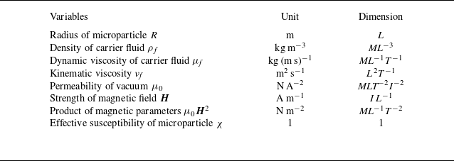
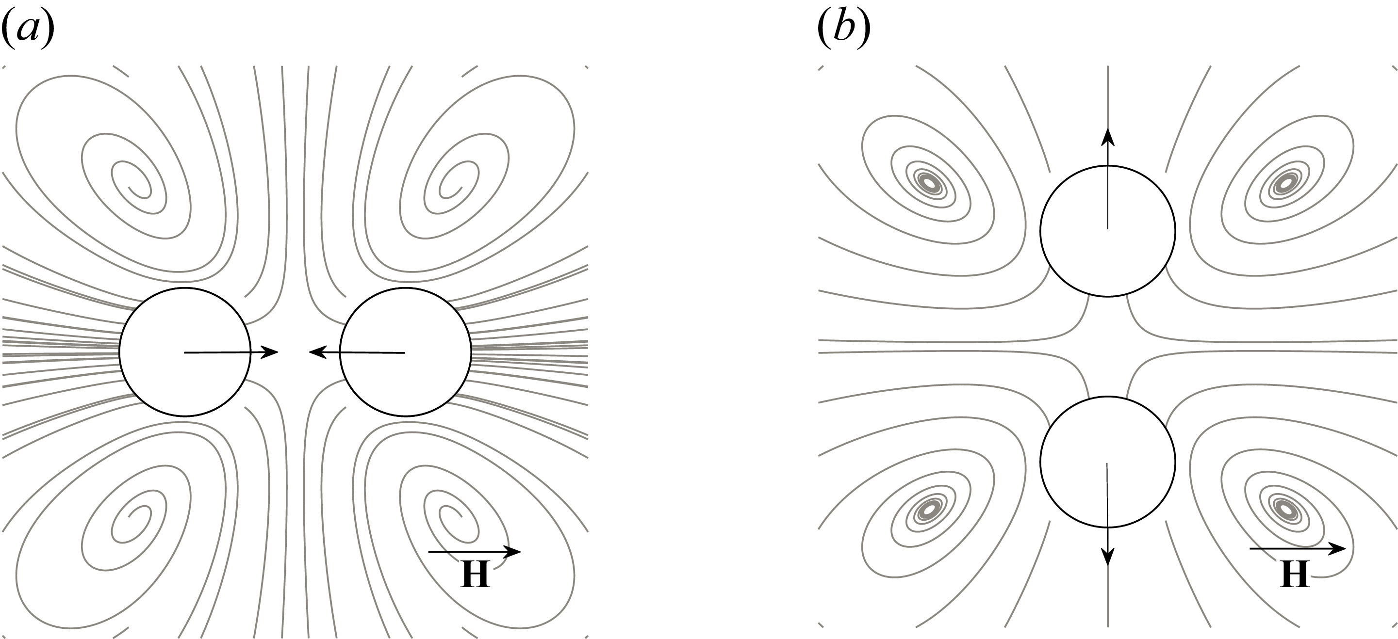


 x

 ×

 ||H||2

 Nmag
 θ=0∘
 θ=20∘
 θ=45∘
 θ=54.7∘
 θ=80∘

 Nmag
 R2/νf
 (R2/νf)/Km
 ρfνf/(μ0χ2H02)

 R/l
 R/l=1/5
 R/l=1/4
 R/l=1/3
 R/l=1/2

 R/l
 θ=0∘
 θ=20∘
 θ=45∘
 θ=54.7∘
 θ=80∘

 τ
 R/l
 τ

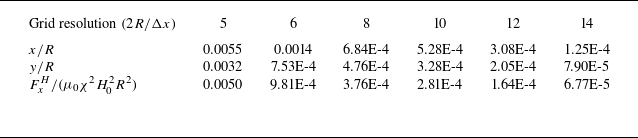
 RMSE
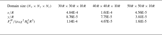
 RMSE



